
Abstract
The urban transport mobility is one of the most important problems for the cities, and involves many aspects that concern to citizens, governments and the economical growth of the countries. Mobility in Mexico City is also a huge problem since the city size makes it insoluble and citizens prefer to use private transportation instead of the public transport network because it offers a poor coverage and a lack of modal transfer centers. With the purpose of analyzing the mobility problems in Mexico City as well as detecting areas of opportunity, the objective of this chapter is to model and simulate the public transportation network from the complex network perspective to asses network structural vulnerability and resilience, considering mobility and accessibility aspects. Firstly, we analyze the urban transport infrastructure in Mexico City taking into account the planning process and sustainability criteria. Secondly, we model and simulate the Mexico City’s public transportation network as a complex network. Thirdly, we characterize the complex network topology of the Mexico City’s public transportation network, and finally we present the main results.
Access provided by CONRICYT-eBooks. Download chapter PDF
Keywords
1 Introduction
“Adding highway lanes to deal with traffic congestion is like loosening your belt to cure obesity.”
Lewis Mumford. The Roaring Traffic’s Boom.
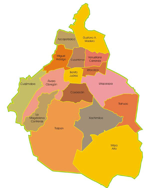
Mexico City is divided by 16 geo-political sectors (see Fig. 1) where each sector has its own government authority. The majority of the Mexican population is urban (78% of total population lives in cities) as in the United States and Brazil (see Table 1). Like many countries around the globe, urban population in Mexico is growing at higher rates compared to the total population, making Mexican cities local engines for national growth [60].

Mexico City sectors, reproduced from http://mapamexicodf360.com.mx/carte/image/es/mapa-delegaciones-mexico.jpg
Varela [60] emphasizes that as competitiveness and growth in Mexican cities are increasingly compromised by congestion, air quality problems, and increased travel times; city officials not only face the challenge of accommodating a growing urban population but also sustaining a constant provision of basic urban services (e.g. clean water, health, job opportunities, transportation, and education). Varela [60] adds that unfortunately, periods of high growth without effective planning and increasing motorization, have pushed Mexican cities towards a “3D” urban growth model: distant, disperse, and disconnected. It is important to note that the 3D model is a direct result of national policies subsidizing housing projects in the outskirts of urban agglomerations, managing urban and rural land poorly, and prioritizing car-oriented solutions for transportation. In consequence, over the past 30 years Mexico City’s population has doubled and its size has increased seven-fold and nowadays it is considered the most populated metropolitan area in the western hemisphere. Table 2 shows some socio-economic KPI’s of Mexico City from 2008 to 2011. Floater et al. [26] Believe that one alternative to the 3D model is the 3C urban growth model: compact, connected and coordinated. In this direction, it is mandatory that a study about urban mobility needs to consider a variety of aspects such as the urban development, the land use, the environmental conditions, the weather, the security, and the social welfare.
Mobility in Mexico City is also a huge problem since the city size makes it insoluble. Mexico City presents the highest congestion level on the road network, causing more than 90% extra travel time for citizens during busy hours. The traffic congestion affects directly on the quality of life, however citizens prefer to use private transportation instead of the public transport network because it offers a poor coverage and a lack of modal transfer centers. Table 3 (at the end of the chapter) shows the mobility KPI’ for Mexico City during 2001, 2007 and 2010.
In the last years, an increasing amount of literature has been devoted to modeling public transportation networks as complex networks [8, 9, 20, 63]. Interesting contributions are found in the literature. For instance, In [61] authors used complex network concepts to analyze statistical properties of urban public transport networks in several major cities of the world. Cheung et al. [20] analyzed the air transportation network in the U.S. Recently Háznagy et al. [33] analyzed the urban public transportation systems of five Hungarian cities performing a comprehensive network analysis of the systems with the main goal of identifying significant similarities and differences of the transportation networks of these cities. Háznagy et al. [33] considered directed and weighted links, where the weights represented the capacities of the vehicles (bus, tram, trolleybus) in the morning peak hours. Reggiani et al. [51] Establishes that the following questions need to be answered with respect to transport networks as complex networks:
-
(a)
Is a complex network a necessary condition for the emergence or presence of transport resilience and vulnerability?
-
(b)
Several indicators of resilience and vulnerability co-exist; are these differences related to specific fields of transportation research?
-
(c)
Can connectivity or accessibility be considered as a unifying framework for understanding and interpreting—in the transport literature—the concepts of resilience and vulnerability?
In this direction, connectivity as the ability to create and maintain a connection between two or more points in a spatial system is one of the essential elements that characterize complex networks. Given the relevance of the connectivity pattern in complex networks, it may seem plausible that complex networks—and connectivity—are a sine qua non for the development of resilience and reduce vulnerability in transportation systems. More recent studies show how the topological properties of a network can offer useful insights into the way a transport network is structured and into the question of which are the most critical nodes (hubs). In this case, resilience and vulnerability conditions associated with such hubs can then affect the resilience/vulnerability of the whole network.
Additionally, Lin and Ban [42] presented the current state of topological research on transportation systems under a complex network framework, as well as the efforts and challenges that have been made in the last decade.
In this chapter, we propose to model and simulate the public transportation network in Mexico City from the complex network perspective to asses’ network structural vulnerability and resilience, considering mobility and accessibility aspects. We consider that a research about the public transportation network in Mexico City should be conducted at different levels. The first one can be done considering the networks as a whole, while the second one should take into account the relationship between geo-political sectors and the third one should analyze each geo-political sector individually. For the purpose of this study, we consider the public transportation network in Mexico City as a whole. In addition, we take into account the lack of connections in the multimodal public transportation network to make some tests based on networks algorithms.
This chapter is divided into five main sections. In Sect. 2, the urban transport infrastructure is analysed considering the planning process and sustainability criteria. In Sect. 3, the complex network modeling and simulation of the Mexico City’s public transportation network is carried out. The complex network topology of the Mexico City’s public transportation network is characterized in Sect. 4. The concluding remarks are drawn in Sect. 5.
Note: Due to the use of the nomenclature of both network theory and graph theory, some authors cited in this chapter use terms such as nodes and vertices to refer to the same, as well as arcs and edges.
2 Urban Transport Infrastructure
Nowadays one of the biggest problems in cities is the transportation system and its infrastructure. There has been a lost of studies and research in recent decades trying to find solutions. In general, there is an economic impact when countries make an investment in this sector. Most of the studies on transportation infrastructure, in particular, focus on its impact on economic growth. In the past two decades, the analytical literature has grown enormously with studies carried out using different theoretical approaches, such as a production function (or cost) and growth regressions, as well as different variants of these models (using different data, methods and methodologies). The majority of these studies have found that transportation infrastructure has a positive effect on output, productivity or economic growth rate [16]. For instance, Aschauer [3] in his empirical study provided substantial evidence that public transport is an important determinant of economic performance. Another example is the study of Alminas et al. [1], who found that transport in general has contributed to growth in the Baltic region.
Another study on the Spanish plan to extend roads and railways that connect Spain with other countries concludes that these have a positive impact in terms of Gross Domestic Product [2]. In a study of the railroad in the United States, it was mentioned that many economists believe that the project costs exceed the benefits [6]. However, the traditional model of cost-benefit assessment does not include the impact of development projects [23].
In these studies focused on growth, we see there is a bias towards economic rather than social goals. That is why it is important to emphasize the impact of transport infrastructure on development and not just growth. Transport infrastructure has to deal with accessibility, mobility and traffic mainly, but if we want to establish a sustainable public transport, is important to consider factors as, economy, land use, trips, environment and social welfare. According to The City of Calgary [57] we divide the urban transport infrastructure as follows:
-
Transportation Planning
-
Transportation Optimization
-
Transportation Simulation
Transportation planning covers many different aspects and is an essential part of the socio-economic system. According to Levy [41], “Most regional transport planners employ what is called the rational model of planning. The model considers planning as a logical and technical process that uses the analysis of quantitative data to decide how to best invest resources in new and existing transport infrastructure.”
Phases for Transportation Planning
There are three phases: The first, preanalysis, considers what problems and issues the region faces and what goals and objectives it can set to help address those issues. The second phase is technical analysis. The process involves the development of the models that are going to be used later. The post-analysis phase involves plan evaluation, program, implementation and monitoring of the results, [35].
Transportation planning involves the following steps:
-
Monitoring existing conditions;
-
Forecasting future population and employment growth, including assessing projected land uses in the region and identifying major growth corridors;
-
Identifying current and projected future transportation problems and needs and analyzing, through detailed planning studies, various transportation improvement strategies to address those needs;
-
Developing long-range plans and short-range programs of alternative capital improvement and operational strategies for moving people and goods;
-
Estimating the impact of recommended future improvements to the transportation system on environmental issues, including air quality; and
-
The development of a financial plan to ensure sufficient income to cover the costs of implementing strategies.
In order to consider these aspects is important to study them into an urban infrastructure scope [25].
Urban Infrastructure
Urban infrastructure, a human creation, is designed and directed by architects, civil engineers, urban planners among others. These professionals design, develop and implement projects (involved with the structural organization of cities and companies) for the proper operation of important sectors of society. When governments are responsible for construction, maintenance, operation and costs, the term “urban infrastructure” is a synonym for public works. Road infrastructure is the set of facilities and equipment used for roads, including road networks, parking spaces, traffic lights, stop signs laybys, drainage systems, bridges and sidewalks. Urban infrastructure includes transportation infrastructure, which in turn, can be divided into three categories: land, sea, and air, they can be found in the following modalities:
The problem in the case of Mexico City is the fragmented government that makes more difficult to implement strategies for plans. This is shown in next Fig. 2.

Governance system for public transport in Mexico City, from [60]
“Such institutional and operational fragmentation has significant implications especially for users. In Buenavista—an area of Mexico City where three modes of transport converge—travelers must walk up to 1.5 km to transfer from one mode to another. About 150,000 people use this disconnected transport hub everyday”
2.1 Transportation Analysis
Manage and plan the services of cities entails a lot of work and participation of experts in different areas. Such is the case of transport that currently represents a challenge for researchers from different areas. There are three measures used for transportation analysis: traffic, mobility and accessibility [43]. As is observed in Fig. 3, the aspects taken into account to compare the three measures are definition of transportation, unit of measure, modes considered, assumptions concerning what benefits consumers, consideration of land use and favored transport improvement strategies (Fig. 4).

Modal connection in Buenavista, adapted from [60]

Comparing transportation measurements, reproduced from [43]
Litman [43] defines these three measures as follows:
Traffic Definition
Traffic refers to vehicle movement. This perspective assumes that “travel” means vehicle travel and “trip” means vehicle-trip. It assumes that the primary way to improve transportation system quality is to increased vehicle mileage and speed.
Mobility Definition
Mobility refers to the movement of people or goods. It assumes that “travel” means person- or ton-miles, “trip” means person- or freight-vehicle trip. It assumes that any increase in travel mileage or speed benefits society.
Accessibility Definition
Accessibility (or just access) refers to the ability to reach desired goods, services, activities and destinations (collectively called opportunities). Access is the ultimate goal of most transportation, except a small portion of travel in which movement is an end in itself (jogging, horseback riding, pleasure drives), with no destination. This perspective assumes that there may be many ways of improving transportation, including improved mobility, improved land use accessibility (which reduce the distance between destinations), or improved mobility substitutes such as telecommunications or delivery services.”
For transportation analysis it is important to consider diverse measures that are used for it, and according to the selected method, different results are obtained. In this chapter we use three different measures in order of importance according to the level of analysis in three levels; macro, mezzo and micro as it will be explained below. It is important to note that sustainability and quality of life of the inhabitants are priority for any proposal or alternative arises.
2.2 Sustainable Urban Transport Infrastructure
According to HABITAT [31] mean by sustainable mobility the following:
Sustainable Urban Mobility: The goal of all transportation is to create universal access to safe, clean and affordable transport for all that in turn may provide access to opportunities, services, goods and amenities. Accessibility and sustainable mobility is to do with the quality and efficiency of reaching destinations whose distances are reduced rather than the hardware associated with transport. Accordingly, sustainable urban mobility is determined by the degree to which the city as a whole is accessible to all its residents, including the poor, the elderly, the young, people with disabilities, women and children. Moreover quality of life and sustainability corresponds to [30]:
In its original definition, sustainable development focuses on “meeting the needs of the present without compromising the ability of future generations to meet their own needs” [45]. The fulfillment of needs is not only a precondition for sustainable development but also for individual well-being and thus for a high quality of life. Quality of life is most commonly defined as consisting of two parts, the objective (the resources and capabilities that are given for a person) and the subjective (the well-being of a person).
There are some sustainable and environmental friendly transport indicators recommended [46] as reported by the European Environmental Agency (EEA) in Copenhagen suggests that appropriate environmental indicators should be able to respond to the following simple questions: what is actually happening of environmental change? is it related to (significant) policy goals? is progress possibly measurable? moreover, how does overarching welfare development influenced? important criteria to select suitable indicators that are both descriptive, able to measure performance as well as progress, are thus that they are:
-
Policy relevant, consisting of parameters that actually might be influenced by policy and administration;
-
Accessible for measuring and comparison—over time or in space; in goals versus results;
-
Representative and valid¸ covering a broad scope of the environmental problems at stake;
-
Reliable and, based on accessible data, of high quality with regular updating;
-
Simplified, able to manage and reduce complex relationships;
-
Informative in order to promote an improved policy performance and broader understanding of the environment transport relationships.
Drawing on well-established international indicator sets on environment and transport, ideal and possible (accessible) indicators are discussed, and an indicator for environmentally friendly urban transport is suggested, divided in five main areas: driving forces, transport factors, environmental factors, urban and societal impacts from transport, urban planning, policies and measures (Fig. 5).

From [46]
Indicators for urban transport, environment and climate.
Other authors offer a slight different view about indicators as Paz et al. [49] that points out: Numerous studies have established different measures to quantify sustainability [64]. According to Bell and Morse [7], sustainability primarily is measured by means of three components: (i) time scale, (ii) spatial scale, and (iii) system quality. The time and spatial scale corresponds to the analysis period and the geographical region of interest, respectively. On the other hand, system quality corresponds to the quantification of the overall system performance or state. In order to quantify system quality, Sustainability Indicators (SIs) have been developed in a diverse range of fields, including biology and the life sciences, hydrology, and transportation.
It is clear that a truly sustainable state for a system requires all the relevant interdependent subsystems/sectors and components, at levels so that the consumption of and the impact on the natural and economic resources do not deplete nor destroy those resources. Hence, the assessment of a system state requires a holistic analysis in order to consider all the relevant sectors and impacts. [49].
As Paz et al. [49] say the analysis should be holistic, and we agree with it, just the approach is different since they propose a study of a system of systems and use fuzzy logic for qualitative indicators.
2.3 The Public Transport Network in Mexico City Context
Mexico City like all other cities has very specific features as the subsoil conditions, and the geographical location; as it is a seismic zone and is filmed by mountains, has two nearby volcanoes and was a lake 1500 years ago. So everything with regard to infrastructure, urban development and air as quality water have to be considered in a study on mobility. The following maps show aspects such as subsoil, environmental pollution and transport networks that exist today, without considering the private public transport networks. This information is important since a sustainable urban development has to consider all the variables that affect the city growing.
Seismic zones are shown in the Fig. 6.

Seismic zones in Mexico City.
These zones were defined in order to regulate buildings construction, [4]. According to the Building Regulations for the Federal District and its Technical Standards Complementary pair Design and Construction of Foundations (2004), Mexico City is divided from the geotechnical point of view in three zones as can be observed in the map, and defined as follows:
-
(a)
Zone I. Lomas, formed by rocks or soil generally firm that were deposited outside the lacustrine environment, but where there may be superficially or interleaved, sandy deposits loose state or relatively soft cohesive. In this area, the presence of voids is common in rocks, caves and excavated soil to exploit sand mines and tunnels filled not controlled;
-
(b)
Zone II. Transition, in which deep deposits are 20 meters deep, or less, and which it consists predominantly sandy and sandy silt layers interspersed with layers lacustrine clay; the thickness thereof varies between a few tens of centimeters and meters;
-
(c)
Zone III. Lacustrine, composed of powerful deposits of highly compressible clay, separated by layers with different sandy silt or clay content. These layers are generally fairly sandy compact to very compact and variable thickness from centimeters to several meters.
Lacustrine deposits usually they covered superficially by alluvial soils, dried materials and artificial fillers; the thickness of this set can be greater than 50 m.
Geotechnical anomalies within the lake area. Auvinet [4].
The lake area is far from having uniform characteristics. In this area there are sites easily where the subsoil has identifiable characteristics. It stresses in particular the existence in the historic center of prehispanic thick fillings. Many farms have on the other hand a complex loading history under colonial buildings; some of them have now disappeared, amending substantially the behaviour of the subsoil under the weight of buildings and seismic conditions.
A similar situation occurs along traces of old roads or albarradones, in areas of channels that were filled and places of ancient human settlements established in all islands or partially artificial lakes within the former, known as tlateles (Tlatelolco, Tlahuac, Iztacalco, etc.), without forgetting the chinampas areas. The presence of these abnormalities, often undetected by designers, has been the source of problems of inappropriate behaviour of foundations and damage structural in buildings. The authors of this article are currently working on a micro zoning to bring the risks that may arise locally to build in a certain place and define recommendations to mitigate its consequences.
Other study about flooding was done by the DEVELOP teams in Wise, Virginia, and Saltillo, Mexico, and researches investigated the physical, social and socio-economic aspects of flooding in Mexico City. The project discerned areas most susceptible to flooding and of higher risk based on socio-economic characteristics. The team partnered with CONAGUA (Comisión Nacional del Agua), ITESM (Instituto Tecnológico de Estudios Superiores de Monterrey), and CAALCA (Centro del Agua para América Latina y el Caribe) to assist with decisions and policy making. Next figure shows the result (Fig. 7).

Social vulnerability scores.
Puente [50] states that, a methodology for assessing urban vulnerability rests on two premises: (1) the material conditions of a city are good indicators of vulnerability; (2) the main components of vulnerability can be mapped at the scale of urban neighborhoods. Based on them last step consists on creating a matrix that displays the appropriate indicators (factors) on one axis and the areal units of analysis on the other axe.
For the purposes of this chapter, we just mention some of them.
Another important factor is air pollution in Mexico City, “Environmental pollution is an increasingly serious problem in third world cities. Pollution arises from both fixed and mobile sources. Industrial facilities in the mega-cities of developing countries have rarely been subject to policies of pollution control. Equally important is pollution generated by urban transportation systems, especially those that depend on motor vehicles. In recent years, local authorities have been obliged to put up with crawling traffic, many frequent traffic jams, and other forms of vehicular paralysis. The supposed advantages of flexibility and speed that were associated with motor vehicles are rapidly disappearing. None the less, these cities must live with the permanent costs of neighborhood social disruption and increased pedestrian hazards that have followed in the wake of motorization. Similar problems of overuse and under management have also affected water resources. Lack of treatment facilities has led to the contamination of streams where wastes are deposited and of the associated aquifers [50].”
As observed from Figs. 8, 9, 10 and 11, public transportation network of Mexico City is constituted by other networks.

Metro and Metrobus networks.

Electric bus network

Eco bus line 1.

Eco bus line 2.
3 Complex Network Analysis of the Mexico City’s Public Transportation Network
The analysis of different complex systems is made much easier with the use of networks. Whenever the system can be represented as a network or graph with nodes and arcs, simple algorithms can be used to solve problems inherent to the network. Nodes can represent cities, production centers, intersections of streets, etc. Arcs relate these nodes, these can have a direction or not, capacity limits or also different items or characteristics, in that sense the study of such networks has been done in a multimodal way. In the last few years some authors have opted to change the analysis of a multimodal network to a multilayer network as we will see later. In our case that is about the public passenger transport network in Mexico City, correspond to a multimodal network and composed of networks considering the mode of transport. Moreover, it is a widely known fact that the problems facing this network are huge as well as the complexity of the network itself. According to graph theory, the basic representation of the structure of the complex network can be generalized by the directed (or undirected) graph
where V describes set of nodes (vertices) and E describes set of arcs (edges) that compose the network. Let W = (w ij ) be the adjacency matrix associated to the graph G, so that the edge e ij has weight w ij . A direct graph is defined by differentiating the direction of edges. In contrast, an undirected graph take does not take into account the direction of edges. The weight of edges represents the importance of edges in the network.
Public transportation networks are complex networks whose structure is irregular, distributed, and dynamically evolving in time [5, 13, 17, 54]. On the one hand, as explain Thai et al. [56] the study of structural properties of the underlying network may be very important in the understanding of the functions of a complex systems as well as to quantify the strategic importance of a set of nodes in order to preserve the best functioning of the network as a whole.
The study of the dynamical properties of a complex network is important in understanding the network complexity. As discussed by Criado and Romance [21], complex network analysis focuses on statistical graph measures, and simulation, using a statistical approach to asses network structural vulnerability by measuring the fraction of the vertices or links to be remove before a complete disconnection happens in the network in order to study complex networks. Criado and Romance [21] add that under the perspective of structural vulnerability, two kinds of damages can be considered on error and attack tolerance in complex networks: the removal of randomly chosen vertices (error tolerance) and the removal of deliberately chosen vertices (attack tolerance).
In this section, we model and simulate the public transportation network in Mexico City from the complex network perspective to asses network structural vulnerability and resilience, considering mobility and accessibility aspects.
To model the Mexico City’s public transportation network as a complex network and evaluate their empirical characteristics we used Gephi, and open source software for the visual exploration of complex networks developed since 2008.
Gephi was created by Mathieu Bastian, Sebastien Heymann, and Mathieu Jacomy, and extended by Eduardo Ramos Ibañez, Cezary Bartosiak, Julian Bilcke, Patrick McSweeney, André Panisson, Jeremy Subtil, Helder Suzuki, Martin Skurla, and Antonio Patriarca from Web Atlas. It is suitable for the analysis of all kind of complex networks. For the purpose of this study, we consider the public transportation network in Mexico City as a whole taking into account the trolebus, metro, metro-bus, ecobus, tren ligero and suburbano transportation systems.
It is important to note that the original configuration of public transport networks from the network analysis was L-space, also referred as the space of stops or space of stations, in which stops or stations are vertices. In this way, two vertices are connected on an arbitrary route [42, 53]. In this study, we built a complex network where a node represents a station from the public transportation networks in Mexico whereas a directed arc represents the physical connection between two stations. The weight of an arc represents the physical linear distance between two stations. The complex network consists of 923 nodes and 1203 arcs. The layouts included in Gephi are algorithms that position the nodes in the 2-D or 3-D graphic space. The patterns created, based on the different layouts, emphasis the properties of the structure of networks. For instance, using the force-algorithms the connected nodes tend to be closer, while disconnected nodes tend to be further [38].
The force directed layout optimizes Martin et al. [44]:
where \( x_{i} \) are positions of nodes, \( w_{ij} \) are arcs weights and \( D_{{x_{i} }} \) is the density of edges near \( x_{i} \).Where D xi denotes the density of the points x 1, …, x n near x i . The sum in (2) contains both an attractive and a repulsive term. The attractive term \( \sum\nolimits_{j} {(w_{ij} d(x_{i} ,x_{j} )^{2} )} \) attempts to draw together nodes, which have strong relations via w ij. The repulsive term D xi attempts to push nodes into areas of the plane that are sparsely populated. The minimization in (2) is a difficult nonlinear problem. For that reason, we use a greedy optimization procedure based on simulated annealing Martin et al. [44]. The procedure is greedy in that we update the position of each vertex by optimizing the inner sum \( \sum\nolimits_{j} {(w_{ij} d(x_{i} ,x_{j} )^{2} ) + D_{{x_{i} }} } \) while fixing the positions of the other nodes.
In order to select the pertinent layout in Gephi software (that means random, force atlas, Fruchterman and Reingold [28], Noverlap, OpenOrd, Hu [34]); it is important to take into account the capability of the algorithm to handle the given data (nodes and arcs), the user time constraint, and the structural network properties to analyze.
For our simulation, we have used Force Atlas, Fruchterman and Reingold [28], and Hu [34] algorithms. As Dey and Roy [24] due to Force Atlas algorithm uses different techniques such as degree-dependent repulsive force, Barnes Hut simulation, and adaptive temperatures for their simulation process.
In this direction, Dey and Roy [24] add that the main idea of simulation is that the nodes repulse and the arcs attract. The network layout using Force Atlas algorithm is shown in Fig. 12a.

Mexico City’s public transportation complex network simulation using a Force Atlas, b Fruchterman Reingold, c OpenOrd, and d Yifan Hu algorithms
Fruchterman and Reingold [28] propose to model a continuous network depending on even distribution of the nodes, making arc lengths uniform and reflects inherent symmetry. The network layout using [28] algorithm is shown in Fig. 12b.
Cherven [19] notes that the OpenOrd algorithm helps to generate network graphs very fast, and is best suited to very large networks that operate at a very high rate of speed while providing a medium degree of accuracy.
The importance of using OpenOrd algorithm is because it uses edge-cutting, average-link clustering, multilevel graph coarsening, and a parallel implementation of a force directed method based on simulated annealing Martin et al. [44]. An advantage of this algorithm over Fruchterman and Reingold [28] one is that for large graphs is the running time, Fruchterman and Reingold [28] is O(n2) in the number of nodes n, The running time can be improved using a grid based density calculation, and by employing a multilevel approach Martin et al. [44].
The goal of OpenOrd is to draw G in two dimensions. Let x i = (x i ,1, x i ,2) denote the position of v i in the plane. OpenOrd draws G by attempting to solve Eq. (2).
All nodes are initially placed at the origin, and the update is repeated for each node in the graph to complete one iteration of the optimization. The iterations are controlled via a simulated annealing type schedule, which consists of five different phases: liquid, expansion, cool-down, crunch, and simmer Martin et al. [44].
During each stage of the annealing schedule, authors vary several parameters of the optimization: temperature, attraction, and damping. These parameters control how far nodes are allowed to move. At each step of the algorithm, they compute two possible node moves. The first possible move is always a random jump, whose distance is determined by the temperature. The second possible move is analytically calculated (known as a barrier jump22). This move is computed as the weighted centroid of the neighbors of the vertex. The damping multiplier determines how far towards this centroid the vertex is allowed to move and the attraction factor weights the resulting energy to determine the desirability of such a move. Of these two possible moves, we choose the move which results in the lowest inner sum energy \( \sum\nolimits_{j} {(w_{ij} d(x_{i} ,x_{j} )^{2} ) + D_{{x_{i} }} } \) (Part of Eq. 2).
OpenOrd uses simulated annealing to solve the problem of Eq. (2). The network layout using OpenOrd algorithm is shown in Fig. 12c.
As Cherven [19] states, Fruchterman and Reingold [28] algorithm produces faster results compared to other force-directed methods by focusing on attraction and repulsion at the neighborhood (rather than the entire network) level. The network layout using Yifan Hu algorithm is shown in Fig. 12d.
3.1 Statistical Graph Measures of the Mexico City’s Public Transportation Complex Network
According to complex networks framework is necessary to have some measures as centrality ones, in order to answer the question “What is the most important or central node in a given network?” Centrality measures (defined below) are the most basic and frequently used methods for analysis of complex networks Tarapata [56].
Based on this, here is a list of some statistical graph measures from Eq. (3) to Eq. (9) to evaluate the empirical characteristics of the Mexico City’s public transportation complex network mostly based on Dey and Roy [24] and Tarapata [55].
Mean Degree
Degree \( k_{i} \) is defined as the number of links connected to the node. The mean degree represents the average degree of all nodes in a network.
where \( \left| V \right| = N \) the average degree calculated was 2.607 (Fig. 13).

Mexico City’s distribution degree for complex public transport network
Connectivity and Accessibility
According to Rodrigue et al. [52], accessibility is defined as the measure of the capacity of a location to be reached by, or to reach different locations therefore, the capacity and the structure of transport infrastructure are key elements in the determination of accessibility. Following Rodrigue et al. [52], two spatial categories are applicable to accessibility problems: topological accessibility and contiguous accessibility. In the first case, it is related to measuring accessibility in a system of nodes and paths, for instance a transportation network, assuming that accessibility is a measurable attribute significant only to specific elements of the transportation system. In the second case, the measure of accessibility is carried out over a surface, being a measurable attribute of every location, as space is considered in a contiguous manner.
Rodrigue et al. [52] adds that the most basic measure of accessibility involves network connectivity through the degree node. As shown in Table 4, the nodes Bellas Artes and Aquiles Serdan of the Mexico City’s public transportation complex network are the most connected. These nodes are subway stations from line 2 and 7. Based on the average degree calculated, and considering the Mexico City’s public transportation complex network as a whole, this degree was 2.607, that means this kind of network has a low accessibility.
Weighted Degree Distribution
Considering that the weight of an edge represents the physical linear distance between two stations, we calculate the average weighted degree.
The weighted degree of a node is like the degree. It’s based on the number of edge for a node, but ponderated by the weight of each edge. It’s doing the sum of the weight of the edges.
For example, a node with 4 edges that weight 1 (1 + 1+1 + 1 = 4) is equivalent to:
-
a node with 2 edges that weight 2 (2 + 2 = 4) or
-
a node with 2 edges that weight 1 and 1 edge that weight 2 (1 + 1+2 = 4) or
-
a node with 1 edge that weight 4 etc.…
In the Mexico City case and based on the Table 4, the weighted degree is 1539.835 (see Fig. 14).

Mexico City’s public complex transportation network weighted degree distribution
Betweenness Centrality
A node is central if it structurally lies between many other nodes, in the sense that it is transversed by many of the shortest paths connecting pairs of nodes. The betweenness centrality is defined as follows.
where \( p_{l,i,k} \) count of the shortest paths in G between l and k nodes visiting the i-th node, \( p_{l,k} \) count of the shortest path in G between l and k nodes. The higher \( bc_{i} \) value, the better (the i-th node is more important or more central). In order to calculate the betweenness centrality, the Gephi software uses A Faster Algorithm for Betweenness Centrality Brandes [12]. The betweenness centrality distribution is shown in Fig. 15.

Betweenness centrality distribution of Mexico City’s public complex transport network
Eccentricity Distribution
As Hage and Harary [32] states, the eccentricity \( ec_{i} \) of the i-th node is calculated using Eq. (5).
where, \( d_{ij} \) represents the length of the shortest path in G between the i-th, and the j-th node (number of edges on the shortest path from i to j). The lower \( ec_{i} \) value, the better (the i-th node is more important or more central). In order to calculate the eccentricity, the Gephi software uses A Faster Algorithm for Betweenness Centrality Brandes [12]. The eccentricity distribution calculated is shown in Fig. 16.

Eccentricity distribution of Mexico City’s complex public transport network
Average Shortest Paths Length
The average shortest paths length L denotes the average minimum distance between any two nodes. The lower L value is the better Watts et al. [62]. In this case, the average path length of the network was 23.611 km.
Diameter
The diameter D represents the maximum path between any two nodes of the network. The lower value D is the better Hage and Harary [32].
In the case of Mexico City’s public transportation complex network, the diameter is 77 segments.
Clustering Coefficient
The local clustering coefficient \( gc_{i} \) of a node i expresses how the neighbors of two adjacent nodes have a link in between Watts et al. [62]. The average clustering C is calculated as follows.
Here, \( E_{i} \) count the edges between first-neighbours of the i-th node. The higher \( gc_{i} \) value, the better (the i-th node is more central). The average clustering coefficient was calculated using Gephi software, based on the algorithm proposed by Latapy [40], and is equal to 0.033. Figure 17 shows the clustering coefficient distribution of the Mexico City’s public transportation complex network.

Clustering coefficient distribution of the Mexico City’s public complex transport network
4 Complex Network Topology of the Mexico City’s Public Transportation Network
4.1 Topology of the Mexico City’s Public Transportation Network
Hubs Distribution
The hubs are nodes with much higher degrees than the average node degree. The occurrence of hubs tends to form clusters in the network. It is important to note that the hubs distribution is assessed in Gephi software based on the algorithm of Kleinberg [37]. The hubs distribution of Mexico City’s public transportation complex network is shown in Fig. 18.

Hubs distribution of Mexico City’s public complex transport network
Authority Distribution
The authority is defined as nodes with the smaller degrees than the average node degree. The authority distribution is also assessed in Gephi software based on the algorithm of Kleinberg [37]. The authority distribution of Mexico City’s public transportation complex network is shown in Fig. 19.

Authority distribution for Mexico City’s public complex transportation network
Modularity
Fortunato and Castellano [27] describe the modularity as the decomposition of the networks into sub-units or communities, which are sets of highly inter-connected nodes. Following Blondel et al. [10], the identification of such communities is of crucial importance as they help to uncover a priori unknown functional modules. As Fortunato and Castellano [27] explain: identify modules and their boundaries allow a classification of vertices, according to their topological position in the modules. In this direction, vertices with a central position in their cluster may have an important function, for instance, control and stability within the group, while vertices at the boundaries between modules play the role of mediation between different communities. Modularity analysis using Gephi software is based on the algorithm proposed by Blondel et al. [10]. It is important to note that the communities detection in graphs is based only on the topology. In the case of Mexico City’s public transportation complex network, the modularity is 0.895 and 29 communities were detected. Figure 20 shows the size distribution of the communities detected in the Mexico City’s public transportation complex network.

Communities distribution size detected in the Mexico City’s public complex transportation network
4.2 Assessment of Structural Vulnerability and Resilience of Mexico City’s Public Transportation Complex Network Based on Simulation
According to Criado and Romance [21], under the perspective of structural vulnerability, two types of damage can be considered on error and attack tolerance in complex networks: the removal of randomly chosen nodes (error tolerance) and the removal of deliberately chosen nodes (attack tolerance). To analyze the resilience of the Mexico City’s public transportation complex network, we remove nodes, which correspond to the stations of the trolebus, metro, metro-bus, ecobus, trenligero and suburbano transportation systems, and edges, which correspond to the physical distance between stations. We chose them both randomly and deliberately. In the Mexico City’s public transportation complex network, eliminating 20% of stations randomly from the network (see Fig. 21), the average degree calculated reduces from 2.607 to 2.488 and the average weighted degree from 1539.835 to 1450.403.

Simulation of Mexico City public complex transportation network using Fruchterman Reingold algorithm, by eliminating 20% of edges randomly
Eliminating 30% of the highest degree nodes from the network (see Fig. 22), the average degree calculated reduces from 2.607 to 1.79 and the average weighted degree from 1539.835 to 1068.313. It is important to note that resilience and vulnerability conditions associated with the hubs can then affect the resilience/vulnerability of the whole network.

Simulation of Mexico City public complex transportation network using Fruchterman Reingold algorithm, by eliminating 30% of the highest degree nodes
4.3 Multimodal Networks and Multilayer Networks
Krygsman et al. [39] observe that much of the effort associated with public transport trips is performed to simply reach the system and the final destination. In this sense, access and exit stations (together with wait and transfer times) are the weakest part of a multimodal public transport chain and their contribution to the total travel disutility is often substantial [11].
Access and exit determine, importantly, the availability (or the catchment area) of public transport [11, 45, 47]. Generally, an increase in access and egress (time and/or distance) is associated with a decrease in the use of public transport [18, 48].
In this direction, two scenarios are observed: in the first one, if access and egress exceed an absolute maximum threshold; users will not use the public transport system, while in the second one, if the access and egress trip components are acceptable, users may use the system, however; much will depend on the convenience of the system. Therefore, we consider that making public transport attractive, safe, self-sustaining and efficient to users is a task that must consider several aspects that are often over looked in studies of this type. Some of the factors that have not been considered are the connection between modes of transportation, which have to do with cycling, walking or using some short-route transport. This has to do with land use, climate and distance.
Due to the complexity of the system and considering the different transport modes and networks involved, it is important to take into account the complete study of such networks as has been shown in the previous sections. As [29] mentioned: “A few studies only considered many modes merged in an unique network, but this aggregation might hide important structural features due to the intrinsically multilayer nature of the network”.
In particular, in the case of urban transport, not considering the connection times can lead to imprecise estimates for the network’s navigability. We note also that interchanges are not symmetrical: rail-to-bus and bus-to-rail waiting time are different and are independent from the actual traffic volume (at least as long as capacity limits are not taken into account). In addition, the existence of alternative trajectories on different transportation modes enhances the system resilience”.
Therefore considering Kivela et al. [36] terminology: “A graph (i.e. a single-layer network) is a tuple G = (V, E), where V is the set of nodes and E ⊆ V × V is the set of edges that connect pairs of nodes. If there is an edge between a pair of nodes, then those nodes are adjacent to each other. This edge is incident to each of the two nodes, and two edges that are incident to the same node are said to be ‘incident’ to each other.
In our most general multilayer-network framework, we allow each node to belong to any subset of the layers, and we are able to consider edges that encompass pairwise connections between all possible combinations of nodes and layers. (One can further generalize this framework to consider hyper edges that connect more than two nodes.) That is, a node u in layer α can be connected to any node v in any layer β. Moreover, we want to consider ‘multidimensional’ layer structures in order to include every type of multilayer network construction that we have encountered in the literature.”
In the case of Mexico City Public Transport, each mode is a layer and networks are connected by the stations that they share, as we show in Fig. 23.

Mexico City multilayer network. Layers represent public transport networks
This figure displays a part of the metro network and only metrobus stations that have connection with it, however these connections are mainly in the central area of Mexico City. This figure shows more clearly the need to analyze the problem as a Multi-layer network, not all layers are considered since there is more means of public transport.
Layer α represents Metro stations, while layer β represents Metrobus stations, and they are connected with other modes of public transport.
In a multilayer network, we need to define connections between pairs of node-layer tuples. As with monoplex networks, we will use the term adjacency to describe a direct connection via an edge between a pair of node-layers and the term incidence to describe the connection between a node-layer and an edge.
Two edges that are incident to the same node-layer are also ‘incident’ to each other. We want to allow all of the possible types of edges that can occur between any pair of node-layers—including ones in which a node is adjacent to a copy of itself in some other layer as well as ones in which a node is adjacent to some other node from another layer. In normal networks (i.e. graphs), the adjacencies are defined by an edge set E ⊆ V × V, in which the first element in each edge is the starting node and the second element is the ending node. In multilayer networks, we also need to specify the starting and ending layers for each edge. We thus define an edge set EM of a multilayer network as a set of pairs of possible combinations of nodes and elementary layers. That is, EM ⊆ VM × VM.
Using the components that we set up above, we define a multilayer network as a quadruplet M = (VM, EM, V, L). [36].
For the general analysis is important to take into account the connectivity not only by layer but intra layers, and how to consider strategies that create a resilient network.
In this way, Demeester et al. [22] set up some objectives for an integrated approach to multilayer survivability that includes:
-
Avoiding contention between the different single-layer recovery schemes
-
Promoting cooperation and sharing of spare capacity
-
Increasing the overall availability that can be obtained for a certain investment budget
-
Decreasing investment costs required to ensure a certain survivability target
This analysis will be done in other chapter since there are more models and details that are not possible to develop properly in this one.
5 Concluding Remarks and Future Work
An important fact to consider for this study is that in terms of mobility citizens in Mexico City prefer to use private instead of public transportation causing the highest congestion level on the road network at global level affecting the quality of life of all citizens because they spend 90% extra travel time during busy hours.
In this chapter we have mentioned the mobility and accessibility of public transport in Mexico City, as well as its connectivity, vulnerability and resilience. It is important to note that this research goes beyond what has been exposed here.
According to some studies, the public transportation network in Mexico City is considered as distance, disperse, and disconnected having a negative effect on the productivity and the economic growth rate of the city. The main motivation of this work was to assess the Mexico City public transportation network structural vulnerability and resilience for detecting areas of opportunity.
This first approach allows us to make a general diagnosis to build later scenarios that allow us to take into account the other aspects of the problem, such as security, environmental impact, land use, climate and traffic.
The results obtained from the simulation model allowed us to conclude that public transportation in Mexico City have features of complex networks whose structure is irregular, distributed and dynamically evolving in time.
The study of structural properties of Mexico City public transportation network allowed us to quantify the strategic importance of a set of nodes (stations) to preserve the functioning of the network as a whole. In order to carry out the assessment we modeled and simulated the network using Gephi software. Our simulations were executed using Force Atlas, Fruchterman Reingold, OpenOrd, and Yifan Hu algorithms.
On the one hand, we observed that the network had a low accessibility because the average degree is low, 2.607. It means that it has a low capacity to be reached by different locations. On the other hand, when the 20% of the total nodes were randomly eliminated to test the resilience of the network, the average degree reduces from 2.607 to 2.488. While eliminating the 30% of the highest degree nodes, the average degree reduces to 1.79. In conclusion, Mexico City public transportation network also presents high vulnerability.
The importance of having this research is that measures to take make the public transport an attractive option against the private one.
References
Alminas, M., Vasiliauskas, A. V., & Jakubauskas, G. (2009). The impact of transport on the competitiveness of national economy. Department of Transport Management, 24(2), 93–99.
Álvarez-Herranz, A., & Martínez-Ruíz, M. P. (2012). Evaluating the economic and regional impact on national transport and infrastructure policies with accessibility variables. Transport, 27(4), 414–427.
Aschauer, D. A. (1991). Transportation spending and economic growth: The effects of transit and highway expenditures. Report. Washington, D.C.: American Transit Association.
Auvinet, G., Méndez, E., Juárez, M., & Rodríguez, J. F. (2013). Geotechnical risks affecting housing projects in Mexico valley. México: Sociedad Mexicana de Mecánica de Suelos.
Bagler, G. (2008). Analysis of the airport network of India as a complex weighted network. Physica A: Statistical Mechanics and its Applications, 387(12), 2972–2980.
Balaker, T. (2006). Do economists reach a conclusion on rail transit? Econ Journal Watch, 3(3), 551.
Bell, S., & Morse, S. (2008). Sustainability indicators: Measuring the immeasurable (2nd ed.). London, UK: Earthscan.
Barabási, A., & Abert, R. (1999). Emergence of scaling in random networks. Science, 286(5439), 509–512.
Berche, B., Ferber, C. V., Holovatch, T., & Holovatch, Y. (2012). Transportation network stability: A case study of city transit. Advances in Complex Systems, 15(supp01), 1–18.
Blondel, V. D., Guillaume, J. L., Lambiotte, R., & ELefebvre, E. (2008). Fast unfolding of communities in large networks. Journal of Statistical Mechanics: Theory and Experiment (10).
Bovy, P. H. L., Jansen, G. R. M. (1979). Travel times for disaggregate travel demand modelling: a discussion and a new travel time model. In G. R. M. Jansen, et al. (Eds.), New Developments in modelling travel demand and urban systems (pp. 129–158). Saxon House, England.
Brandes, U. (2001). A faster algorithm for betweenness centrality. Journal of Mathematical Sociology, 25(2), 163–177.
Buckwalter, D. W. (2001). Complex topology in the highway network of Hungary, 1990 and 1998. Journal of Transport Geography, 9(2), 125–135.
CAF. (2011a). Desarrollo urbano y movilidad en América Latina and INEGI 2013.
CAF. (2011b). Desarrollo urbano y movilidad en América Latina. CTSEMBARQ México, Based on 2007 mobility survey. Estadísticas SETRAVI. Fideicomiso para el mejoramiento de lasvías de DF. 2001. Secretaría del MedioAmbiente. 2008. Inventario de emisiones de la ZMVM, 2006.
Calderón, C., & Servén, L. (2008). Infrastructure and economic development in Sub-Saharan Africa. The World Bank Policy Research Working Paper, 4712.
Caschili, S., & De Montis, A. (2013). Accessibility and complex network analysis of the US commuting system. Cities, 30, 4–17.
Cervero, R. (2001). Walk-and-ride: Factors influencing pedestrian access to transit. Journal of Public Transportation, 3(4), 1–23.
Cherven, K. (2015). Mastering Gephi network visualization. Birmingham: Packt Publishing.
Cheung, D. P., & Gunes, M. H. (2012). A complex network analysis of the United States air transportation. In Proceedings of the 2012 IEEE/ACM International Conference on Advances in Social Networks Analysis and Mining, 26–29 August 2012 (pp. 699–701). Istanbul, Turkey: Kadir Has University 2012.
Criado, R., & Romance, M. (2012). Optimization and its applications. In M. T. Thai & P. M. Pardalos (eds.), Handbook of optimization in complex networks: Communication and social networks (Vol. 58). Springer. doi:10.1007/978-1-4614-0857-41.
Demeester, P., & Michael, G. (1999). Resilience in multilayer networks. IEEE Communications Magazine, 0163-6804/99.
De Rus, G. (2008). The economic effects of high speed rail investment. University of Las Palmas, Spain, Discussion Paper, 2008-16.
Dey, P., & Roy, S. (2016). A comparative analysis of different social network parameters derived from Facebook profiles. In S. C. Satapathy, et al. (Eds.), Proceedings of the Second International conference on Computer and Communication Technologies. Advances in Intelligent Systems and Computing (Vol. 379).
Flores I., Mújica, M., & Hernández, S. (2015). Urban transport infrastructure: A survey. In EMSS 2015 Proceedings, Bergeggi, Italy.
Floater, G., & Rode, P. (2014). Cities and the new climate economy: the transformative role of global urban growth. In The new climate economy: The transformative role of global urban growth, November 2014. http://newclimateeconomy.net/.
Fortunato, S., & Castellano, C. (2007). Community structure in graphs. arXiv:0712.2716.
Fruchterman, T. M. J., & Reingold, E. M. (1991). Graph drawing by force-directed placement. Software—Practice & Experience, 21(11), 1129–1164.
Galloti, R., & Barthelemy, M. (2014). Anatomy and efficiency of urban multimodal mobility. Scientific Reports, 4, 6911. doi:10.1038/srep06911.
Grünberger, S., & Omann, I. (2011). Quality of life and sustainability. Links between sustainable behaviour, social capital and well-being. In 9th Biennial Conference of the European Society for Ecological Economics (ESEE): “Advancing Sustainability in a Time of Crisis” from 14th to 17th June 2011, Istanbul, Turkey.
HABITAT. (2015). http://www.gob.mx/sedatu/documentos/reglas-de-operacion-del-programa-habitat-2015. Reporte Nacional de la Movilidad Urbana en México 2014–2015.
Hage, P., & Harary, F. (1995). Eccentricity and centrality in networks. Social Networks, 17(1), 57–63.
Háznagy, A., Fi, I., London, A., & Tamas, N. (2015) Complex network analysis of public transportation networks: A comprehensive study. In 2015 Models and Technologies for Intelligent Transportation Systems (MT-ITS), 3–5 June 2015. Budapest, Hungary.
Hu, Y. F. (2005). Efficient and high quality force-directed graph drawing. The Mathematica Journal, 10, 37–71.
Johnston, R. A. (2004). The urban transportation planning process. In S. Hansen, & G. Guliano (Eds.), The Geography of Urban Transportation. Multi-modal transportation planning (pp. 115–138). The Guilford Press.
Kivelä, M., et al. (2014). Multilayer networks. Journal of Complex Networks, 2, 203–271.
Kleinberg, J. M. (1999). Authoritative sources in a hyperlinked environment. Journal of the ACM, 46(5), 604–632.
Kobourov, S. G. (2012). Force-directed drawing algorithms. In Handbook of graph drawing and visualization. CRC Press.
Krygsman, S., Dijsta, M., & Arentze, T. (2004). Multimodal public transport: An analysis of travel time elements and the interconnectivity ratio. Transport Policy, 11(2004), 265–275.
Latapy, M. (2008). Main-memory triangle computations for very large (Sparse (Power-Law)) graphs. Theoretical Computer Science (TCS), 407(1–3), 458–473.
Levy, J. M. (2011). Contemporary urban planning. Boston: Longman.
Lin, J., & Ban, Y. (2013). Complex network topology of transportation systems. Transport Reviews, 33(6), 658–685. doi:10.1080/01441647.2013.848955.
Litman, T. (2011). Measuring transportation traffic, mobility and accessibility. Victoria Transport Policy Institute. http://www.vtpi.org, Info@vtpi.org.
Martin, F., & Boyack, K. (2011). OpenOrd: An open-source toolbox for large graph layout. In Proceedings of SPIE—The International Society for Optical Engineering, January 2011.
Murray, A. T. (2001). Strategic analysis of public transport coverage. Socio-Economic Planning Sciences, 35, 175–188.
Nenseth, V., & Nielsen, G. (2009). Indicators for sustainable urban transport—state of the art. TØI report 1029/2009.
Ortúzar, J.d.D., Willumsen, L.G., 2002. Modelling Transport, third ed, Wiley, West Sussex, England.
O’Sullivan, S., & Morrall, J. (1996). Walking distances to and from light-rail transit stations. Transportation Research Record, 1538.
Paz, A., Maheshwari, P., Kachroo, P., & Ahmad, S. (2013). Estimation of performance indices for the planning of sustainable transportation systems. Hindawi Publishing Corporation. Advances in Fuzzy Systems, 2013, Article ID 601468, 13 pp.
Puente, S. (1999). Social vulnerability to disasters in Mexico City: An assessment method. In J. K. Mitchell (Eds.), Crucibles of hazard: Mega-cities and disasters in transition (pp. 296–297). Tokyo New York, Paris: United Nations University Press.
Reggiani, A., Nijkamp, P., & Lanzi, D. (2015). Transport resilience and vulnerability: The role of connectivity. Transportation Research Part A, 81, 4–15.
Rodrigue, J.-P., Comtois, C., & Slack, B. (2009). The geography of transport systems. New York, NY: Routledge.
Sienkiewicz, J., & Holyst, J. A. (2005). Statistical analyses of 22 public transport networks in Poland. Physical Review E, 72, 046127.
Shen, B., & Gao, Z.-Y. (2008). Dynamical properties of transportation on complex networks. Physica A: Statistical Mechanics and its Applications, 387(5), 1352–1360.
Tarapata, Z. (2015). Modelling and analysis of transportation networks using complex networks: Poland case study. The Archives of Transport, 4(36), 55–65.
Thai, My. T., & Pardalos, P. M. (2012). Handbook of optimization in complex networks. Springer.
The City of Calgary, Transportation Department. Retrieved 8 March, 2015, from http://www.calgary.ca/Transportation/Pages/Transportation-Department.aspx.
Tsay, S., & Herrmann, V. (2013). Rethinking urban mobility: Sustainable policies for the century of the city (68 pp.). Washington, DC: Carnegie Endowment for International Peace.
UN Documents Gathering a Body of Global Agreements. (1987). Our common future, Chapter 2. In Towards sustainable development. United Nations Decade of Education for Sustainable Development in a Creative Commons, Open Source Climate. Geneva, Switzerland, June 1987.
Varela, S. (2015). Urban and suburban transport in Mexico City: Lessons learned implementing BRTs lines and suburban railways for the first time. Integrated Transport Development Experiences of Global City Clusters, International Transport Forum, 2–3 July 2015, Beijing China.
Von Ferber, C., Holovatch, T., Holovatch, Y., & Palchykov, V. (2009). Public transport networks: Empirical analysis and modeling. The European Physical Journal B, 68(2), 261–275.
Watts, D. J., & Strogatz, S. H. (1998). Collective dynamics of ‘small-world’ networks. Nature, 393(6684), 440–442.
Zanin, M., & Lillo, F. (2013). Modelling the air transport with complex networks: A short review. The European Physical Journal Special Topics, 215(1), 5–21.
Zheng, J., Atkinson-Palombo, C., McCahill, C., O’Hara, R., & Garrick, N. W. (2011). Quantifying the economic domain of transportation sustainability. In Proceedings of the Annual Meeting of the Transportation Research Board CDROM, Washington, DC, USA.
Acknowledgements
This research was supported by UNAM-PAPIIT grant IT102117.
Author information
Authors and Affiliations
Corresponding author
Editor information
Editors and Affiliations
Rights and permissions
Copyright information
© 2017 Springer International Publishing AG
About this chapter
Cite this chapter
Flores De La Mota, I., Huerta-Barrientos, A. (2017). Simulation-Optimization of the Mexico City Public Transportation Network: A Complex Network Analysis Framework. In: Mujica Mota, M., Flores De La Mota, I. (eds) Applied Simulation and Optimization 2. Springer, Cham. https://doi.org/10.1007/978-3-319-55810-3_2
Download citation
DOI: https://doi.org/10.1007/978-3-319-55810-3_2
Published:
Publisher Name: Springer, Cham
Print ISBN: 978-3-319-55809-7
Online ISBN: 978-3-319-55810-3
eBook Packages: Mathematics and StatisticsMathematics and Statistics (R0)