Vortices and Rotation

Abstract

As well as being free from viscosity, the Bose–Einstein condensate has another striking property—it is constrained to circulate only through the presence of whirlpools of fixed size and quantized circulation. In contrast, in conventional fluids, the eddies can have arbitrary size and circulation. Here we establish the form of these quantum vortices, their key properties, and how they are formed and modelled.

These keywords were added by machine and not by the authors. This process is experimental and the keywords may be updated as the learning algorithm improves.

5.1 Phase Defects

The condensate’s wavefunction is a complex quantity. We have seen that it can be written as $\varPsi (\mathbf{r},t)=R(\mathbf{r},t)e^{i S(\mathbf{r},t)}$ (Madelung transform), where $R(\mathbf{r},t)$ and $S(\mathbf{r},t)$ are respectively the phase and amplitude distributions at time t. Consider following a closed path C of arbitrary shape through a region of the condensate. As we go around the path, the integrated change in the phase is

$$\begin{aligned} \varDelta S = \oint _C \nabla S \cdot \mathrm{d}{\varvec{\ell }}, \end{aligned}$$

(5.1)

where the vector d${\varvec{\ell }}$ is the line element of integration. Let the wavefunction be $\varPsi _0$ and $\varPsi _1$ respectively at the starting point and at the final point of C. Since the two points are the same and $\varPsi$ must be single-valued, the condition $\varPsi _1=\varPsi _0$ means that,

$$\begin{aligned} \varDelta S =2\pi q, \qquad q=0,\pm 1, \pm 2, \ldots \end{aligned}$$

(5.2)

If the integer number $q \ne 0$ then, somewhere within the region enclosed by C, there must be a phase defect, a point where the phase wraps by the amount $2\pi q$. At this point the phase of the wavefunction takes on every value, and the only way that $\varPsi$ can remain single-valued here is if $\varPsi$ is exactly zero.

5.2 Quantized Vortices

What does the presence of a phase defect mean for the condensate as a fluid? Recalling that the phase distribution defines the fluid’s velocity via $\mathbf{v}=(\hbar /m) \nabla S$, Eq. (5.2) implies that the circulation $\varGamma$ around the path C is either zero or a multiple of the quantum of circulation $\kappa$,

$$\begin{aligned} \varGamma =\oint _C \mathbf{v} \cdot \mathrm{d}{\varvec{\ell }}= q \kappa , \qquad \kappa =\frac{h}{m}. \end{aligned}$$

(5.3)

This important result (the quantization of the circulation ) tells us that the condensate flows very differently from ordinary fluids, where the circulation takes arbitrary values.

Assume that $q \ne 0$, and that the path C is a circle of radius r centred at the singularity. Consider the simple case of two-dimensional flow in the xy plane. Using polar coordinates $(r, \theta )$, the line element is $\mathrm{d}{\varvec{\ell }}=r \mathrm{d}\theta ~{\widehat{\varvec{e}}}_{\theta }$, where ${\widehat{\varvec{e}}}_{\theta }$ is the unit vector in the azimuthal direction $\theta$. Then the circulation becomes,

$$\begin{aligned} \varGamma =\oint _C \mathbf{v} \cdot \mathrm{d}{\varvec{\ell }}= \int ^{2\pi }_0 r \mathbf{v} \cdot {\widehat{\varvec{e}}}_{\theta }~ \mathrm{d}\theta = 2\pi r v_{\theta }. \end{aligned}$$

(5.4)

Comparison with Eq. (5.3) shows that the fluid’s azimuthal speed around the singularity is,

$$\begin{aligned} v_{\theta }=\frac{q\hbar }{m r}=\frac{q \kappa }{2 \pi r}. \end{aligned}$$

(5.5)

Since the condensate is a fluid without viscosity, this flow around the singularity should go on forever, at least in principle!

For $q\ne 0$, Eq. (5.5) tells us that the velocity around the singularity decreases to zero at infinity ($v_{\theta } \rightarrow 0$ as $r \rightarrow \infty$), and that, as we approach the axis, the flow becomes faster and faster, and diverges ($v_{\theta } \rightarrow \infty$ as $r \rightarrow 0$). If we increase q, the flow speed increases discontinuously, because q takes only discrete values. The sign of q determines the direction of the flow (clockwise or anticlockwise) around the singularity.

We now have a better picture of the nature of the singularity: it is a quantized vortex line, a whirlpool in the fluid. The quantity q is called the charge of the vortex . Figure 5.1 (left) represents a straight vortex line through the origin, parallel to the z axis. Since the flow is the same on all planes perpendicular to the z axis, the flow of the (three-dimensional) straight vortex can be more simply described as the flow due to a two-dimensional vortex point on the xy plane, as in Fig. 5.1 (middle). If these conditions are not met, such as the curved vortex line shown in Fig. 5.1 (right), then the flow is fully three-dimensional and cannot be represented by a vortex point.

Fig. 5.1

Left Schematic (three-dimensional) straight vortex line through the origin and parallel to the z axis. The red tube around the vortex axis of radius $a_0$ represents the vortex core. Middle Since the vortex line is straight, it suffices to consider the two-dimensional flow of a vortex point on the xy plane (the flow on other planes parallel to the xy plane will be the same). Right For a more general bent vortex line the flow is fully three-dimensional

5.3 Classical Versus Quantum Vortices

The flow of the condensate is different from the flow of an ordinary fluid in two respects. Firstly, and as we showed in Sect. 3.3, it is inviscid (there is no viscosity to slow down the flow and bring it to a stop). Secondly, the circulation is quantized, as we showed above. To appreciate the second difference we recall the vorticity field (the local rotation), defined as,

$$\begin{aligned} {\varvec{\omega }}=\nabla \times \mathbf{v}. \end{aligned}$$

(5.6)

The following examples illustrate velocity fields with the associated vorticity fields:

• (i) Consider water inside a bucket rotating at constant angular velocity $\varOmega$. We use cylindrical coordinates $(r,\theta ,z)$ where z is the axis of rotation.¹ The velocity field is $\mathbf{v}=v_{\theta }{\widehat{\varvec{e}}}_{\theta }= \varOmega r{\widehat{\varvec{e}}}_{\theta }$ and the vorticity is ${\varvec{\omega }}=2 \varOmega {\widehat{\varvec{e}}}_z$ (where ${\widehat{\varvec{e}}}_{\theta }$ and ${\widehat{\varvec{e}}}_z$ are the unit vectors along $\theta$ and z). The azimuthal speed $v_{\theta }$ of this flow as a function of r is shown by case (i) of Fig. 5.2a. This flow is called solid body rotation.

• (ii) As derived above, the velocity field around a vortex line in a condensate is $v_{\theta }=q\hbar /(m r)$, shown by case (ii) in Fig. 5.2a. It is easy to verify that its vorticity is zero: we say that this flow is irrotational. Physically, a parcel of fluid which goes around the vortex axis does not ‘turn’ (as it does in solid body rotation), but retains its orientation (like a gondola of a Ferris wheel); this flow is depicted in case (ii) of Fig. 5.2b. The property of irrotationality also follows mathematically: the condensate’s velocity is proportional to the gradient of the quantum mechanical phase, and the curl of a gradient is always zero. However, the singularity itself contributes vorticity according to ,

  $$\begin{aligned} {\varvec{\omega }}= \kappa \delta ^2(\mathbf{r}) {\widehat{\varvec{e}}}_{z}, \end{aligned}$$

  (5.7)

  where $\delta ^2(\mathbf{r})$ is the two-dimensional delta function satisfying $\delta ^2(\mathbf{r}=0)=1$ and $\delta ^2(\mathbf{r}\ne 0)=0$. At first it may surprise that a quantum vortex has zero vorticity, but the result is expected—the key point is that motion in the condensate is irrotational, but isolated vortex line singularities are allowed.

• (iii) The velocity of the wind around the centre of a hurricane, case (iii) of Fig. 5.2a, combines solid body rotation in the inner region ($r \ll a_0$) with irrotational motion in the outer region ($r \gg a_0$) where $a_0$ is called the vortex core radius.

Fig. 5.2

a Examples of rotation curves. (i) solid body rotation, (ii) vortex line in a condensate (irrotational flow), and (iii) flow around a hurricane or a bathtub vortex, which combines solid body rotation in the inner region $r \ll a_0$ and irrotational flow in the outer region $r\gg a_0$. b Schematic of the two-dimensional flow for cases (i) and (ii), showing the orientation of an object, here a leaf, in the flow

In ordinary fluids the vorticity ${\varvec{\omega }}$ is arbitrary, and therefore vortices can be weak or strong, big or small. In a condensate, Eq. (5.3) is a strict quantum mechanical constraint: motion around a singularity has fixed form and intensity.

Fig. 5.3

a The radial density profile n(r) of a $q=1$ vortex in a homogeneous condensate (solid line). Shown for comparison is the ‘healing’ profile for a static condensate whose density is pinned to zero. b Appearance of a vortex lying along the axis of a trapped condensate. Shown is an isosurface of the 3D density (with the vortex appearing as a central tube), a 2D density profile column integrated along z (with the vortex appearing as a black dot), and a 1D density profile column-integrated along y and z

5.4 The Nature of the Vortex Core

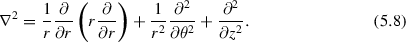
A natural question is: what is the structure of the vortex, particularly towards the axis of the vortex ($r \rightarrow 0$), where, according to Eq. (5.5), the velocity becomes infinite? Using cylindrical coordinates $(r,\theta ,z)$ again, we consider a straight vortex line aligned in the z direction in a homogeneous condensate ($V=0$). Assuming $\varPsi (r,\theta ,z)=A(r) e^{i q \theta }$ and substituting into the GPE of Eq. (3.9) we obtain the following differential equation,² for the function A(r),

$$\begin{aligned} \mu A=-\frac{\hbar ^2}{2m} \frac{1}{r} \frac{\mathrm{d}}{\mathrm{d}r} \left( r \frac{\mathrm{d} A}{\mathrm{d}r}\right) +\frac{\hbar ^2 q^2}{2 m r^2} A + g A^3, \end{aligned}$$

(5.9)

The terms on the right-hand side arise from the quantum kinetic energy, the kinetic energy of the circulating flow and the interaction energy, respectively. The boundary conditions are that $A(r) \rightarrow 0$ for $r \rightarrow 0$ and $A(r) \rightarrow \psi _0$ for $r \rightarrow \infty$. The equation has no exact solution and must be solved numerically for A(r); the corresponding density profile $n(r)=A^2$ is shown in Fig. 5.3a. It is apparent that the axis of the vortex is surrounded by a region of depleted density, essentially a tube of radius $a_0 \approx 5 \xi$, called the vortex core radius. For small r, the density scales as $r^{|q|}$. We see that although the velocity diverges for $r \rightarrow 0$, the density vanishes—no atom moves at infinite speed! We can therefore interpret a vortex as a ‘hole’ surrounded by (quantized) circulation. Recall from Sect. 3.4.2 that if a static and otherwise homogeneous condensate is pinned to zero density, then the density ‘heals’ back to the background density with a characteristic profile $\tanh ^2(x/\xi )$. The vortex density profile is slightly wider than this profile and relaxes more slowly to the background density, as seen in Fig. 5.3a. This is due to the kinetic energy of the circulating flow, which gives rise to an outwards centrifugal force on the fluid.

While there is no exact analytic form for the vortex density profile, a useful approximation for a single-charged vortex is,

$$\begin{aligned} n(r)=n_0\left( 1-\frac{1}{1+r'^2} \right) , \end{aligned}$$

(5.10)

where $r'=r/\xi$.

This result (a vortex line is a ‘hole’ surrounded by circulating flow) has an interesting mathematical consequence: a condensate with vortices is a multiply-connected region, and the classical Stokes Theorem³ does not apply.

In a trapped condensate the vortex creates a similar tube surrounded by quantised circulation; the only difference is that the density of the condensate is not uniform (as in a homogeneous condensate). In typical 2D column-integrated images of the condensate, the vortex appears as a low density dot. Since the healing length depends on the local density, in a trapped condensate the thickness of the vortex core depends on the position. If the condensate is in the Thomas–Fermi regime and the vortex along the z axis, then an approximation for the density profile can be constructed as the product of the static Thomas–Fermi profile, Eq. (3.33), and the vortex density, Eq. (5.10), i.e.,

$$\begin{aligned} n(x,y,z)=n_0\left( 1-\frac{x^2}{R_x^2} -\frac{y^2}{R_y^2} -\frac{z^2}{R_z^2}\right) \left( 1-\frac{1}{1+r'^2} \right) , \end{aligned}$$

(5.11)

where $r'=r/\xi$ is defined is terms of the healing length evaluated at the condensate centre.

5.5 Vortex Energy and Angular Momentum

We now evaluate some useful properties associated with a quantum vortex: its energy and angular momentum. For simplicity, we still consider the case of a single straight vortex lying along the z-axis of a cylindrically-symmetric condensate of constant density; assuming that the condensate’s size is much larger than the healing length, the density depletion at the axis of the vortex and near the walls can be neglected. A cylindrical bucket of height $H_0$ and radius $R_0$ containing superfluid liquid helium would be a realistic example. For trapped atomic condensates, where the vortex size is significant relative to the system size and the condensate density varies in space, these ideas can be generalized by, for example, taking the density profile to be of the form of Eq. (5.11), or by estimating the necessary integrals numerically.

The kinetic energy $E_\mathrm{kin}$ of the swirling fluid is obtained from summing the contributions of the atoms, each carrying kinetic energy $m v_{\theta }^2/2$ where $\mathbf{v}=v_{\theta } {\widehat{\varvec{e}}}_{\theta } =(q \hbar /mr)~{\widehat{\varvec{e}}}_{\theta }$ is the velocity. Summing over all atoms we have,

$$\begin{aligned} E_\mathrm{kin}=\int \frac{1}{2} m n(\mathbf{r}) v_{\theta }^2(\mathbf{r})~\mathrm{d}^3\mathbf{r}, \end{aligned}$$

(5.12)

where the integral is performed over the bucket’s volume. Using cylindrical coordinates,

$$\begin{aligned} E_\mathrm{kin}=\int _0^{H_0} \mathrm{d}z \int _0^{2 \pi } \mathrm{d}\theta \int _0^{R_0} \frac{m n_0}{2} \left( \frac{q \hbar }{m r}\right) ^2~r~\mathrm{d}r =\pi H_0 \frac{n_0 q^2 \hbar ^2}{m} \int _0^{R_0} \frac{\mathrm{d}r}{r}. \end{aligned}$$

(5.13)

To prevent the integral from diverging at $r \rightarrow 0$ we introduce a cutoff length $a_0$,⁴ the vortex core radius; in doing so, we recognize that the density vanishes at the axis of the vortex, but simplify the core structure, assuming that the core is hollow up to the distance $r=a_0$. Notice that without the outer limit of integration (the size of the container $R_0$) the integral would also diverge at $r \rightarrow \infty$. We then obtain,

$$\begin{aligned} E_\mathrm{kin}=\pi H_0 \frac{n_0 q^2 \hbar ^2}{m} \int _{a_0}^{R_0} \frac{\mathrm{d}r}{r} =\pi H_0 \frac{n_0 q^2 \hbar ^2}{m} \ln \left( \frac{R_0}{a_0} \right) . \end{aligned}$$

(5.14)

We conclude that the kinetic energy per unit length of the vortex, $E_\mathrm{kin}/H_0=\pi n_0 (q^2 \hbar ^2/m)\ln {(R_0/a_0)}$, is constant.

Each atom swirling around the axis of the vortex carries angular momentum $L_z=m v_{\theta }r$. The total angular momentum of the flow is therefore,

$$\begin{aligned} L_z=\int m n (\mathbf{r}) v_{\theta } (\mathbf{r}) r~\mathrm{d}^3 \mathbf{r}. \end{aligned}$$

(5.15)

Proceeding as for the kinetic energy, we find,

$$\begin{aligned} L_z= 2 \pi H_0 n_0 q \hbar \left( \frac{R_0^2}{2} - \frac{a_0^2}{2} \right) \approx \pi H_0 n_0 q \hbar R_0^2. \end{aligned}$$

(5.16)

Consider a condensate in a state with an arbitrary high angular momentum $L_z$. We can construct this state as either (i) one vortex with large q or (ii) many vortices with $q=1$. Which situation is preferred? Since $E_\mathrm{kin}$ scales as $q^2$, a state with many singly-charged vortices has less energy than a state with a single multi-charged vortex. Experiments confirm that this is indeed the case: in Ref. [1] a $q=2$ vortex was seen to quickly decay into two singly-charged vortices. Hereafter we assume that all vortices are singly-charged, with $q=\pm 1$.

5.6 Rotating Condensates and Vortex Lattices

5.6.1 Buckets

Vortices are easily created by rotating the condensate [22, 23]. Consider again a cylindrical condensate of height $H_0$, radius $R_0$ and uniform density. A vortex appears only if the system, by creating a vortex, lowers its energy. In a rotating system at very low temperature, it is not the energy E which must be minimized, but rather the free energy $F=E-\varOmega L_z$ where $\varOmega$ is the angular velocity of rotation. A state without any vortex, hence without angular momentum, has free energy $F_1=E_0$ where $E_0$ is the internal energy. A state with a vortex has free energy $F_2=E_0+E_\mathrm{kin}-\varOmega L_z$. The free energy difference is thus,

$$\begin{aligned} \varDelta F=F_2-F_1=E_\mathrm{kin}-\varOmega L_z= 2 \pi H_0 \frac{\hbar ^2}{m^2} \ln \left( \frac{R_0}{a_0} \right) -\varOmega \pi H_0 n_0 \hbar R_0^2. \end{aligned}$$

(5.17)

Therefore $\varDelta F<0$ (the free energy is reduced by creating a vortex) provided that the rotational velocity is larger than a critical value $\varOmega _{c1}$,

$$\begin{aligned} \varOmega > \varOmega _{c1}=\frac{\hbar }{m R_0^2} \ln \left( \frac{R_0}{a_0} \right) . \end{aligned}$$

(5.18)

For superfluid helium ($m=6.7\times 10^{-27}$ kg, $\kappa =9.97 \times 10^{-8}\,\mathrm {m^2/s}$, $a_0 \approx 10^{-10}\,\mathrm m$) inside a container of radius $R_0=10^{-2}\,\mathrm m$, the critical angular velocity is $\varOmega _{c1}=3\times 10^{-3}\,\mathrm s^{-1}$. States with two, three and more vortices onset at higher critical velocities $\varOmega _{c2}$, $\varOmega _{c3}$ etc., as shown in Fig. 5.4 for superfluid helium and in Fig. 5.7 for atomic condensates. Note that the vortices are parallel to the rotation axis and arrange themselves in a vortex lattice like atoms in a crystal with triangular symmetry . The vortex lattice is therefore a steady configuration in the frame of reference rotating at angular velocity $\varOmega$.

Vortices are topological defects which can only be created at a boundary or spontaneously with an oppositely-charged vortex.⁵ Where then do the vortices in a vortex lattice originate from?

For a rotating container of helium, with even a relatively small rotation frequency, the roughness of the container surface is expected to seed vortices, providing a constant source of vortices from which to develop a vortex lattice in the bulk if the critical rotation frequency is exceeded.

Fig. 5.4

Experimental images of vortex lattices at increasing angular velocities $\varOmega$ in superfluid helium. Reprinted figure with permission from [3]. Copyright 1979 by the American Physical Society

According to Feynman’s rule, the density of vortices (number of vortices per unit area) is,

$$\begin{aligned} n_v=\frac{2 \varOmega }{\kappa }. \end{aligned}$$

(5.19)

Since each vortex contributes vorticity according to Eq. (5.7), the average vorticity per unit area is,

$$\begin{aligned} \bar{{\varvec{\omega }}} = \kappa n_v {\widehat{\varvec{e}}}_z = 2 \varOmega {\widehat{\varvec{e}}}_z. \end{aligned}$$

(5.20)

This tells us that the averaged vorticity (averaged over distance larger than the inter-vortex spacing) reproduces the vorticity $2 \varOmega$ of an ordinary fluid in rotation. Similarly, the large-scale azimuthal flow is $\mathbf{v} \approx \varOmega r {\widehat{\varvec{e}}}_{\theta }$. Remarkably, the many quantized vortices mimic classical solid body rotational flow. Note that the local velocity field around vortices can remain rather complicated.

In the frame rotating at angular frequency $\varOmega$ about the z-axis, the GPE of Eq. (3.46) is ,

$$\begin{aligned} i \hbar \frac{\partial \psi }{\partial t}= -\frac{\hbar ^2}{2m}\nabla ^2 \psi + g \vert \psi \vert ^2 \psi + V \psi + \varOmega L_z \psi - \mu \psi , \end{aligned}$$

(5.21)

where,

$$\begin{aligned} L_z=i \hbar \left( y \frac{\partial }{\partial x} - x \frac{\partial }{\partial y}\right) , \end{aligned}$$

(5.22)

is the angular momentum operator in the z direction . The vortex lattices are the ground-state stationary solutions of this equation (providing $\varOmega$ is large enough). Figure 5.5 shows such a vortex lattice solution for a condensate being rotated in a bucket. The above bucket scenario is modelled through the bucket potential,

$$\begin{aligned} V(r)= \left\{ \begin{array}{lr} 0 &{} \quad \mathrm{~if~} r \le R_0,\\ \infty &{} \quad \mathrm{~if~} r > R_0. \end{array} \right. \end{aligned}$$

(5.23)

The lattice features $N_\mathrm{v}=56$ vortices. Note the appearance of the phase “dislocations” in the phase profile at each vortex position. At the boundary there are as many $2 \pi$ phase slips as there are vortices. The average flow speed around the edge of the bucket can then be approximated by evaluating the magnitude of $\mathbf{v}=(\hbar /m)\nabla S$ around the boundary, i.e.,

$$\begin{aligned} v_r(r=R_0)=\frac{\hbar }{m}\frac{2 \pi N_\mathrm{v}}{2 \pi R_0} = \frac{\hbar }{m}\frac{56}{29 \xi } \approx 1.93 c. \end{aligned}$$

(5.24)

This is close to what one would expect for solid body rotation, $v_r(r=R_0) = \varOmega R_0= 2.3 c$ .

Fig. 5.5

Vortex lattice formed in a bucket potential rotating about the z-axis. Shown are the a density (in arbitrary units) and b phase (in units of $\pi$) in the xy-plane (position presented in units of the healing length $\xi$), corresponding to the stationary solution of the rotating-frame GPE of Eq. (5.21). The bucket has radius $R=29 \xi$ and the rotation frequency is $\varOmega =0.08\, c/\xi$. Image courtesy of Thomas Winiecki [2]

In a small system, at the same value of $\varOmega$ one often observes vortex configurations which are slightly different from each other. This is because there is a very small energy difference between these slightly rearranged states. For example, Fig. 5.4 shows two states with six vortices each (in one case the six vortices are distributed around a circle, in the other case there are five vortices around a circle and one vortex in the middle).

Notice how the background density for the rotating bucket solution in Fig. 5.5 features a meniscus, that is, it is raised towards the edge of the bucket. Let us determine this background density profile. We denote the rotation vector ${\varvec{\Omega }}=\varOmega {\widehat{\varvec{e}}}_z$.

Recall the fluid interpretation of the GPE. Using the Madelung transformation $\psi =\sqrt{n}e^{iS}$ and the fluid velocity definition $\mathbf{v}=(\hbar /m)\nabla S$, the rotating-frame GPE of Eq. (5.21) is equivalent to the modified fluid equations ,

$$\begin{aligned} \dfrac{\partial n}{\partial t}= & {} -\nabla \cdot \left[ n\left( \mathbf{v}-{\varvec{\Omega }}\times \mathbf{r}\right) \right] , \end{aligned}$$

(5.25)

$$\begin{aligned} \displaystyle m \frac{\partial \mathbf{v}}{\partial t}= & {} - \nabla \cdot \left( \frac{1}{2}mv^2+ V+ gn - \frac{\hbar ^2}{2m} \frac{\nabla ^2 \sqrt{n}}{\sqrt{n}}- m \mathbf{v}\cdot \left[ {\varvec{\Omega }}\times \mathbf{r} \right] \right) , \end{aligned}$$

(5.26)

where the ${\varvec{\omega }}\times \mathbf{r}$ terms account for frame rotation and $\mathbf{v}$ is the velocity field in the laboratory frame (expressed in the coordinates of the rotating frame). We assume the Thomas–Fermi approximation by neglecting the quantum pressure term in Eq. (5.26), and seek the stationary density profile. Setting $\partial \mathbf{v}/\partial t=0$ and integrating gives,

$$\begin{aligned} \frac{1}{2}mv^2+ V+ gn - m \mathbf{v}\cdot \left[ {\varvec{\Omega }}\times \mathbf{r} \right] = \mu , \end{aligned}$$

(5.27)

where the chemical potential $\mu$ is the integration constant.

We consider a coarse-grained scale, ignoring the structure of the individual vortices and for which the velocity field approximates the solid body form $\mathbf{v}(r)=\varOmega r {\widehat{\varvec{e}}}_\theta$. We then obtain,

$$\begin{aligned} gn +V - \frac{1}{2}m \varOmega ^2 r^2 = \mu , \end{aligned}$$

(5.28)

where we have used ${\widehat{\varvec{e}}}_z \times {\widehat{\varvec{e}}}_r={\widehat{\varvec{e}}}_\theta$. Rearranging for the density,

$$\begin{aligned} n(r)= \frac{1}{g}\left( \mu -V+ \frac{1}{2}m \varOmega ^2 r^2 \right) , \end{aligned}$$

(5.29)

which is valid for $n(r)>0$; otherwise $n(r)=0$. We conclude that rotation causes a parabolic increase in the coarse-grained density, consistent with the behaviour visible in Fig. 5.5. The is due to centrifugal effects, and is observed in rotating classical fluids. Note that $\mu$ can be determined by normalizing the profile to the required number of atoms or average density.

5.6.2 Trapped Condensates

To predict the critical rotation frequency for vortices to become favoured in a harmonically-trapped condensate, one can repeat the above approach but the inhomogeneous density profile must be accounted for (i.e. replacing $n_0$ above with $n(\mathbf{r})$). One way to approximate this is by the Thomas–Fermi density profile. For a trap which is symmetric in the plane of rotation, with frequency $\omega _\perp$, the critical rotation frequency is then,

$$\begin{aligned} \varOmega _\mathrm{c1} = \frac{5}{2} \frac{\hbar }{m R_\perp ^2} \ln \left( \frac{0.67 R_\perp }{\xi }\right) , \end{aligned}$$

(5.30)

where $R_\perp$ is the Thomas–Fermi radius in the plane of rotation. For typical atomic condensates, $\varOmega _\mathrm{c1}\sim 0.3 \omega _\perp$ .

Rotating an axi-symmetric harmonic trap applies no torque to the condensate, and so in practice the trap is made slightly anisotropic in the plane of rotation in order to form a vortex lattice. Surprisingly, experiments observed vortices at rotation frequencies $\varOmega \sim 0.7 \omega _\perp$, considerably higher than the frequency at which they become energetically favourable. The traps are so smooth that vortex nucleation is very different to that of helium.

Fig. 5.6

a Illustration of the irrotational flow pattern of a rotating elliptically-trapped condensate, according to Eq. (5.31). The color indicates the phase S(x, y) while the velocity field is shown by arrows. b The velocity field amplitude $\beta$ as a function of rotation frequency $\varOmega$ for an axi-symmetric trap ($\epsilon =0$). At $\varOmega =\omega _\perp /\sqrt{2}$ the solutions trifurcate. In this region, these solutions become unstable

We can examine this by considering the planar potential to be weakly elliptical, with frequencies $\omega _x=\sqrt{1-\epsilon }\omega _\perp$ and $\omega _y=\sqrt{1+\epsilon }\omega _\perp$, where $\epsilon$ is the trap ellipticity . We follow the approaches of Refs. [6, 7]. We seek the stationary solutions of the trapped vortex-free condensate under rotation about z. Under the Thomas–Fermi approximation, the solutions must satisfy Eq. (5.27). Furthermore, we look for solutions with the phase profile, and corresponding velocity profile, given by,

$$\begin{aligned} S(x,y)=\beta xy, \quad \mathbf{v}(x,y)=\frac{\hbar }{m} \nabla S=\frac{\beta \hbar }{m}(y {\widehat{\varvec{e}}}_x + x {\widehat{\varvec{e}}}_y). \end{aligned}$$

(5.31)

where $\beta$ is a parameter to be determined below. Inserting into Eq. (5.27), and noting that ${\varvec{\Omega }}\times \mathbf{r}=\varOmega (x {\widehat{\varvec{e}}}_y-y {\widehat{\varvec{e}}}_x)$, leads to the density profile,

$$\begin{aligned} n=\frac{1}{g}\left( \mu -\frac{1}{2}(m \tilde{\omega }_x^2 x^2+\tilde{\omega }_y^2 y^2 + \omega _z^2 z^2)\right) , \end{aligned}$$

(5.32)

where the effect of the rotation is to introduce effective trap frequencies in the xy-plane,

$$\begin{aligned} \tilde{\omega }_x^2= & {} (1-\epsilon )\omega _\perp ^2+\beta ^2-2\beta \varOmega , \end{aligned}$$

(5.33)

$$\begin{aligned} \tilde{\omega }_y^2= & {} (1+\epsilon )\omega _\perp ^2+\beta ^2+2\beta \varOmega . \end{aligned}$$

(5.34)

Plugging this density profile into the rotating-frame continuity equation, Eq. (5.25), and setting $\partial n/\partial t=0$, leads to an expression for $\beta$,

$$\begin{aligned} \beta ^3+\beta (\omega _\perp ^2-2\varOmega ^2)-\epsilon \varOmega \omega _\perp ^2=0. \end{aligned}$$

(5.35)

Hence the stationary solution of the condensate in the rotating frame has been completely specified. In the laboratory frame, this solution has an elliptical density profile which rotates about z. However, the fluid remains irrotational, thanks to the special velocity field which distorts the density is such a way as to mimic rotation, as depicted in Fig. 5.6 a .

Fig. 5.7

An experimental vortex lattice c formed in a flattened trapped rotating atomic condensate (image represents the condensate density). b shows the profile of the corresponding non-rotating condensate. d and e show the side views of the non-rotating and rotating condensates, respectively. The condensate grew in radius with the number of vortices, as shown in a. Reprinted figure with permission from [5]. Copyright 2001 by the American Physical Society

Analysing the case of $\epsilon =0$ for simplicity, there exists one solution, with $\beta =0$, for $\varOmega \le \omega _\perp /\sqrt{2}$; this represents a motion-less and axi-symmetric condensate. However, for $\varOmega > \omega _\perp /\sqrt{2}$ the solutions trifurcate, with two new branches with $\beta \ne 0$ and corresponding to non-axi-symmetric solutions of the form shown in Fig. 5.6. This trifurcation leads to an instability of the condensate (as can be confirmed via linearizing about these solutions [7]) in which perturbations grow at the condensate surface and develop into vortices. Experiments [8] and simulations [9] of the GPE show that this instability then allows the condensate to evolve into a vortex lattice, the lowest energy state.

Figure 5.7 shows a vortex lattice produced in a rotating trapped atomic condensate. Note the regularity and density of the vortex lattice. Note also that the rotating condensate is significantly broader than the non-rotating condensate. In the presence of the vortex lattice, we can predict the coarse-grained density profile of the condensate. Considering an axi-symmetric trap ($\omega _x=\omega _y\equiv \omega _\perp$), then the coarse-grained density profile of Eq. (5.29) gives,

$$\begin{aligned} n(r)= \frac{1}{g}\left( \mu -\frac{1}{2}m(\omega _r^2 r^2-\varOmega ^2) r^2 \right) . \end{aligned}$$

(5.36)

There is a competition between the quadratic trapping potential, which pushes atoms inwards, and the quadratic centrifugal potential, which pushes atoms outwards. The net potential is quadratic with effective harmonic potential $\omega _r^2-\varOmega ^2$. As $\varOmega$ is increased, the condensate expands, and when $\varOmega \ge \omega _r$ it becomes untrapped!

5.7 Vortex Pairs and Vortex Rings

An important property of a vortex is that it moves with the local fluid velocity, and this means that two vortices in proximity induce each other to move. We now consider some important examples.

5.7.1 Vortex-Antivortex Pairs and Corotating Pairs

Consider a pair of vortices of opposite circulation and separation d, a state called a vortex-antivortex pair or vortex dipole, shown schematically in Fig. 5.8. In the figure, the flow around the vortex at the left is anticlockwise, and the flow around the anti-vortex at the right is clockwise. Each vortex is carried along by the flow field of the other vortex, and at each vortex the flow field has speed $v = \hbar /m d$ acting perpendicular to the line separating the vortices. Moreover, this flow acts in the same direction for both vortices, and hence they propagate together at this speed .

Fig. 5.8

Schematic of a vortex-antivortex pair

If instead the vortices have the same circulation, then the flow which carries each vortex now acts in opposite directions (again, perpendicular to the line separating the vortices and with the above speed). The net effect is for the vortices to co-rotate about their mid-point. The angular frequency of this motion is $\omega =2v/d = 2\hbar /m d^2$. From this simple example, one can imagine how many vortices of the same circulation rotate together in a vortex lattice. Note that the above predictions for the pair speed ignore core effects, and so are only valid for $d \gg a_0$.

We can estimate the energy of the vortex pairs in a cylindrical condensate (radius $R_0$, height $H_0$) by assuming a uniform density and integrating the kinetic energy, as we did to calculate the energy of a single vortex line in Eq. (5.14). The vortices have circulation $q_1$ and $q_2$, and individual velocity fields $\mathbf{v}_1$ and $\mathbf{v}_2$, respectively. The net velocity field of the two vortices is $\mathbf{v}_1+\mathbf{v}_2$. Assuming $\xi \ll d \ll R_0$ then the (kinetic) energy of the pair is,

$$\begin{aligned} E_\mathrm{kin}=\int m n_0 |\mathbf{v}_1+\mathbf{v}_2|^2~\mathrm{d}{} \mathbf{r} = \frac{\pi n_0 H_0 \hbar ^2}{m} \left[ q_1^2 \ln \frac{R_0}{a_0}+q_2^2 \ln \frac{R_0}{a_0}+ 2 q_1 q_2 \ln \frac{R_0}{d} \right] . \end{aligned}$$

(5.37)

The first two terms are the energies of the individual vortices if they were isolated. The second term is the interaction energy, the change in energy arising from the interaction between the vortices. For a vortex-antivortex pair ($q_1=-q_2$) the interaction energy is negative. This is because the flow fields tend cancel out in the bulk, reducing the total kinetic energy. Indeed, in the limit $d \rightarrow a_0$, the flow fields completely cancel and the total energy tends to zero; in reality the vortices annihilate with each other in this limit. For a corotating pair ($q_1=q_2$), the interaction energy is positive; in the bulk the flow fields tend to reinforce, increasing the total kinetic energy.

In the presence of dissipation on the vortices, this result also informs us that vortex-antivortex pairs will shrink (ultimately annihilating when their cores begin to overlap) and corotating pairs will expand. Interestingly, at finite temperature and in 2D condensates, vortex-antivortex pairs can be created spontaneously [10].

5.7.2 Vortex Rings

A vortex line either terminates at a boundary (e.g. the vortex in the cylindrical container discussed in the previous section) or is a closed loop. A circular vortex loop is called a vortex ring. It is the three-dimensional analog of the (two-dimensional) vortex-antivortex pair: each element of the ring moves due to the flow induced by the rest of the ring, resulting in the ring travelling in a straight line at a constant speed which is inversely proportional to its radius. Figure 5.9 shows a vortex ring travelling towards, and interacting with, a straight vortex line.

Both vortex rings and vortex-antivortex pairs are forms of solitary waves, since they propagate without spreading. Moreover, like dark solitons, they are stationary (excited) solutions of the homogeneous condensate in the frame moving with the ring/pair.

Fig. 5.9

Vortex ring travelling towards a vortex line computed by numerically solving the GPE (courtesy of A.J. Youd) in a periodic box (hence the vortex line appears to terminate at the top and at the bottom)

5.7.3 Vortex Pair and Ring Generation by a Moving Obstacle

Vortex rings are easily generated in ordinary fluids by pushing the fluid through an orifice: cigarette smokers, volcanoes and dolphins can make vortex rings. In condensates and helium, rings and vortex-antivortex pairs can be formed by moving obstacles.

To understand this mechanism, recall Landau’s criterion for the generation of excitations in the condensate (Sect. 4.2). In the hydrodynamic picture, the speed of the atom/impurity is replaced by the local fluid velocity . Consider the scenario of a homogeneous condensate flowing with bulk speed $v_\infty$ past a cylindrical obstacle (this is equivalent to the cylindrical obstacle moving at speed $v_\infty$ through a static condensate but more convenient to simulate). For low $v_\infty$, the condensate undergoes undisturbed laminar flow around the obstacle, as shown in Fig. 5.10 (left). Note that the local flow speed is approximately twice as large, i.e. $2v_\infty$ at the poles of the obstacle than it is in the bulk (indeed, for an inviscid Euler fluid one would expect it to be exactly $2v_\infty$). When $v_\infty \approx 0.5 c$, the local flow at the poles exceeds the speed of sound, and, as per Landau’s prediction, excitations are created. These take the form of pairs of opposite circulation vortices, which periodically peal off from the poles of the obstacle and travel downstream, as seen in Fig. 5.10 (right).

Fig. 5.10

Flow of a homogeneous condensate past a cylindrical obstacle, below (left) and above (right) the critical velocity. Shown is the condensate density, and the arrows (left) show the velocity field. Note that the obstacle punches a large hole in the condensate. Results are based on simulations of the 2D GPE in the moving frame. Figure reproduced from Ref. [11] under a CC BY licence

Fig. 5.11

a Experimental images of a vortex-antivortex pair moving within a trapped condensate. b The vortex-antivortex pair’s trajectory is reproduced by numerically solving the GPE. Note that the vortex core appears larger in the experimental images since the condensate is first expanded to aid in resolving the cores. Figure adapted with permission from Ref. [14]. Copyrighted by the American Physical Society. A schematic of the trajectory of a vortex-antivortex pair in a trapped condensate is shown on the right

This process has been studied experimentally in atomic condensates [14, 15]. The obstacle is engineered by a laser beam which exerts a localized repulsive potential on the condensate, and is moved relative to the condensate. Figure 5.11 shows an experimental vortex-antivortex pair which moves within a trapped condensate (top). The dynamics can be reproduced by simulating the GPE (bottom). Note that whereas in an infinite condensate the vortex-antivortex pair has constant translational velocity, within a harmonically-trapped condensate the motion of each vortex of the pair follows a curved trajectory .

Similarly, vortex rings arise when a spherical obstacle exceeds a critical speed relative to the condensate. They can be created in superfluid helium by injecting electrons with a sharp high-voltage tip; the electron’s zero point motion carves a small, charged spherical bubble in the liquid of radius approximately $16 \times 10^{-10}\,\mathrm m$ which can be accelerated by an applied electric field. Upon exceeding a critical velocity, a vortex ring peels off at the bubble’s equator; subsequently the electron falls into the vortex core, leaving a vortex ring with an electron bubble attached; the last part of the sequence is shown in Fig. 5.12 .

Fig. 5.12

Vortex rings nucleated by moving bubbles, computed by numerically solving the GPE. Figure reproduced from [16] with permission from EDP Sciences

5.8 Motion of Individual Vortices

We have seen how vortices move due to their interactions with other vortices. Isolated vortices can also move under a variety of scenarios.

First imagine a condensate in a static bucket with a straight vortex line positioned close to the edge. The fluid velocity must be zero at the boundary. In effect, it is as if an image vortex, with opposite circulation, exists on the other side of the boundary. As such the vortex moves around the boundary of the container as a virtual pair with its image.

In a harmonically-trapped condensate, an off-centre vortex precesses about the trap centre. The slow variation of the density towards the edge complicates an image interpretation. Instead, we can interpret the precession in terms of a Magnus force. Imagine the vortex line as a rotating cylinder, shown in Fig. 5.13 (left). The vortex line feels a radial force due to its position in the condensate, and this gives rise to a motion of the vortex line which is perpendicular to the force, $\mathbf{v_\mathrm{L}}$, an effect well known in classical hydrodynamics. This force can be deduced from the free energy of the system. This energy decreases with the vortex position, $r_0$, as shown in Fig. 5.13 (right). This radial force, which follows as $-\partial E/\partial r_0$, acts outwards and has contributions from the “buoyancy” of the vortex, which behaves like a bubble, as well as its kinetic energy. This force balances the Magnus force $-m n {\varvec{\kappa }} \times \mathbf{v}_L$, leading to the expression,

$$\begin{aligned} \frac{\partial E}{\partial r_0}\widehat{{\mathbf{e}}}_r = m n {\varvec{\kappa }} \times \mathbf{v_L}, \end{aligned}$$

(5.38)

where ${\varvec{\kappa }}$ is the circulation vector. The net effect is a precession of the vortex about the trap centre. More generally, the vortex follows a path of constant free energy; for example, it will trace out a circular path in an axi-symmetric harmonic trap and an elliptical path in a non-axi-symmetric harmonic trap. The experiment of Ref. [18] pioneered the real-time imaging of vortices in condensates and was able to directly monitor the precession of a vortex, finding it to agree well with theoretical predictions .

At the trap centre, $E(r_0)$ becomes flat such that the vortex ceases to precess; in fact, the trapped condensate with a central vortex line is a stationary state. For a non-rotating condensate, this state is energetically unstable ($E(r_0)$ is a maximum at the origin). Under sufficiently fast rotation, however, $E(r_0)$ changes shape such that this state becomes a minimum and thus energetically stable, consistent with discussion in Sect. 5.6.

This analysis assumes the vortex line to be straight. This is valid is flattened, quasi-2D geometries, but in 3D geometries, the vortex line can bend and support excitations.

Fig. 5.13

Left Schematic of the Magnus effect which causes an off-centre vortex to precess in a trapped condensate. Right Free energy E of a trapped condensate versus the radial position of a vortex, $r_0$. The top line is for a non-rotating system, while the lower lines have increasing rotation frequencies. Reprinted figure with permission from [17]. Copyright 1999 by the American Physical Society

5.9 Kelvin Waves

A sinusoidal or helical perturbation of the vortex core away from its rest position is called a Kelvin wave. Figure 5.14 (left) shows a Kelvin wave of amplitude A and wavelength $\lambda$. A Kelvin wave of infinitesimal amplitude A and wavelength $\lambda \gg a_0$ rotates with angular velocity,

$$\begin{aligned} \omega _0 \approx \frac{\kappa k^2}{4 \pi } \left( \ln {\left( \frac{1}{ka_0} \right) } -0.116 \right) , \end{aligned}$$

(5.39)

where $k=2 \pi /\lambda$ is the wavenumber; in other words, the shorter the wave the faster it rotates. The time sequence shown in Fig. 5.9 shows a vortex ring which hits a straight vortex. It is apparent that after the collision the straight vortex is perturbed by Kelvin waves. Vortex rings can also be perturbed by Kelvin waves, see Fig. 5.14 (right); the vortex ring with waves travels slower than the unperturbed circular ring. Vortex lines also support excitations in the form of breathers [19].

Fig. 5.14

Left Schematic of Kelvin waves of amplitude A and wavelength $\lambda$. The three unit vectors in the tangent, normal and binormal directions are shown. The waves rotate along the binormal direction, in the direction opposite to the direction of the flow. Right Comparison between motion of a vortex ring (radius $R=0.1\,\mathrm cm$, blue) and a vortex ring perturbed by Kelvin waves (relative amplitude $A/R=0.05$, red). Calculation performed with the vortex filament model [12]. Figure adapted with permission from Ref. [12]. Copyrighted by the American Physical Society

5.10 Vortex Reconnections

When two quantum vortex lines approach each other, they reconnect, changing the topology of the flow. The effect, illustrated in Fig. 5.15, has been experimentally observed in superfluid helium [20] and in atomic condensates [21]. In classical inviscid fluids (governed by the Euler equation) vortex reconnections are not possible. Reconnections of quantum vortices thus arise from the presence of the quantum pressure term in the Gross–Pitaevskii equation. In classical viscous fluids (governed by the Navier-Stokes equation) reconnections are possible but involve dissipation of energy, whereas in condensates reconnections take place while conserving the energy. Figure 5.16 shows the reconnection of two vortices computed using the GPE. A vortex-antivortex pair, initially slightly bent, propagates to the right. The curvature of the vortices quickly increases at their midpoint, they move faster and hit each other, reconnecting and then moving away .

Fig. 5.15

Schematic vortex reconnection of two vortex lines. The arrows indicate the direction of the vorticity (the rotation of the fluid around the axis of the vortex). Left before the reconnection ($t<t_0)$; Middle at the moment of reconnection, $t=t_0$; Right after the reconnection ($t< t_0$)

Fig. 5.16

Reconnection of antiparallel vortex lines computed by solving the GPE in a periodic box. Shown is the isosurface of the condensate density $\rho =0.2$, where $\rho =1.0$ is the bulk value. Reprinted from [24] with the permission of AIP Publishing

In 2D, vortex reconnections become annihilation events in which two vortex points of opposite polarity destroy each other. This can occur through the interaction with a third vortex, and leaves behind a soliton-like rarefaction pulse of sound [25]. Recently, it has been argued that a fourth vortex is required to turn the rarefaction pulse into sound waves which then spread to infinity [26, 27], making the annihilation a four-vortex process.

5.11 Sound Emission

Even in the absence of thermal effects, vortices can lose energy, and they do so by creating sound waves. This occurs when vortices and vortex elements accelerate, for example, Fig. 5.17 (left) shows the pattern of spiral sound waves emitted outwards by a co-rotating pair of vortices. It also arises during vortex reconnections, which release a sharp pulse of sound, as seen in Fig. 5.17 (right). In 2D annihilation events leave behind only sound waves .

In all of these scenarios, the pattern of the condensate phase changes. The information about this change can travel outwards from the vortices no faster than the speed of sound. Beyond this “information horizon”, the condensate phase has the old pattern. The sound waves act to smooth between the new and old patterns, and prevent discontinuities in the phase at this horizon.

The time evolution of a condensate described by the GPE (that is, a condensate at very small temperatures) conserves the total energy, although the relative proportion of kinetic energy (due to vortices) and sound energy (due to waves) may change. In general, a collection of freely-evolving vortices will decay into sound waves, with the energy being transferred into the “sound field”, although this decay is typically very slow. The decay can be prohibited, or even reversed, by suitable driving of the system, and under certain conditions, intense sound waves can create vortices [29].

Fig. 5.17

Left Pattern of sound waves (density variations) on the xy plane generated by a rotating pair of vortices (shown by the white dots). Image adapted from [28]. Note the small amplitude of the sound waves, relative to the background density of one. Right Rarefaction sound pulse generated by the vortex reconnection of Fig. 5.16, shown as density variations on the central plane. Reprinted from [24] with the permission of AIP Publishing

5.12 Quantum Turbulence

Besides lattices, Kelvin waves and vortex rings, other complex vortex states have been studied recently, e.g., U- and S-shaped vortices [30] and vortex knots [31], see Fig. 5.18. But the most challenging vortex state is turbulence .

Fig. 5.18

Left U and S-shaped vortices in a spheroidal condensate. Reprinted figure with permission from [30]. Copyright 2003 by the American Physical Society. Right The break-up of a $T_{2,3}$ vortex knot into two vortex rings. Reprinted figure with permission from [31]. Copyright 2012 by the American Physical Society

A disordered vortex configuration of many vortices is called a vortex tangle ; it represents a state of quantum turbulence. Vortex reconnections and the resulting generation of smaller and smaller vortex loops in a cascade process were first conjectured by Richard Feynman in his pioneering 1955 article on the applications of quantum mechanics to liquid helium [32]. Figure 5.19 illustrates this cascade. Vortices move in an irregular way around each other, undergoing reconnections which trigger Kelvin waves and generate small vortex loops. In a statistical steady state, the intensity of the turbulence is usually measured (experimentally and numerically) by the vortex line density L, defined as the length of vortex lines per unit volume . From the vortex line density L one estimates that the typical distance between vortices is $\ell \approx L^{-1/2}$. As well as vortices, quantum turbulence also features sound waves.

Fig. 5.19

Schematic of vortex reconnections and generation of small vortex loops, as envisaged by Richard Feynman [32]

Current work [33, 34] studies properties of quantum turbulence such as velocity and acceleration statistics [35], the emergence of coherent structures out of disorder, and the energy spectrum $E_k$ (representing the distribution of the kinetic energy over the length scales); in particular, the energy spectrum is defined from ,

$$\begin{aligned} E'=\frac{1}{\mathcal{V}} \int _\mathcal{V} \frac{\mathbf{v}^2}{2} \mathrm{d}^3\mathbf{r} =\int _0^{\infty } E_k ~\mathrm{d}k, \end{aligned}$$

(5.40)

where $E'$ is energy per unit mass, $\mathcal V$ is the volume and k the wavenumber.

The two main tools to study quantum turbulence are the GPE and the vortex filament model, which we describe in Sect. 5.13; the latter is directly relevant to superfluid helium, but is important in general, as it isolates vortex interactions, neglecting finite core-size effects and sound waves. In the next subsections we describe recent results for 3D and 2D turbulence.

5.12.1 Three-Dimensional Quantum Turbulence

Quantum turbulence at very low temperatures is generated in superfluid helium by stirring with grids, wires or propellers, or by injecting vortex rings . Observations of the decay of the vortex line density and the energy spectrum reveal two turbulent regimes [36]. In the first regime [37], called quasi-classical turbulence and illustrated in Fig. 5.20, the energy spectrum obeys the same Kolmogorov scaling of ordinary turbulence ($E_k \sim k^{-5/3}$) over the hydrodynamic range $k_D \ll k \ll k_{\ell }$ (where $k_{\ell }=2 \pi /\ell$, $k_D=2 \pi /D$ and D is the system size). This result is confirmed by numerical simulations based on the GPE [38] and the vortex filament model [39–41]. Kolmogorov scaling suggests the existence of a classical cascade, which, step-by-step, transfers energy from large eddies to smaller eddies. The concentration of energy at the largest length scales (near $k_D$) arises from the emergence of transient bundles of vortices of the same polarity [42] which induce large scale flows. Without forcing, quasi-classical turbulence decays as $L \sim t^{-3/2}$ .

However, under other conditions, $E_k$ peaks at the intermediate scales followed at large wavenumbers by the $k^{-1}$ dependence typical of isolated vortices, suggesting a random vortex configuration without cascade [41]. In the absence of forcing, this regime, called ultra-quantum turbulence [36], decays as $L \sim t^{-1}$.

Fig. 5.20

a Quantum turbulence in superfluid helium computed in a periodic box using the vortex filament method [42]. Lighter colour denotes bundles of vortex lines with the same orientation: they are responsible for the emergence of the classical $k^{-5/3}$ Kolmogorov spectrum. Figure adapted with permission from Ref. [42]. Copyrighted by the American Physical Society . b Energy spectrum of the kinetic energy $E_k$ vs k, computed using the vortex filament method [40]: note the $k^{-5/3}$ Kolmogorov scaling for $k< k_{\ell } \approx 1.8 \times 10^5\,\mathrm{m^{-1}}$. The curve at the bottom shows that the spectrum of the coarse-grained vorticity is consistent with the $k^{1/3}$ scaling of Kolmogorov theory

Fig. 5.21

Left Absorption images of turbulent 3D atomic condensate (top) and schematic diagram of the inferred distribution of vortices (bottom) [43]. Reprinted figure with permission from [43]. Copyright 2009 by the American Physical Society. Middle Quantum turbulence in a harmonically confined atomic condensate computed using the GPE. The surface of the condensate is pale blue, the surface of the vortex cores is purple. Figure adapted with permission from Ref. [35]. Copyrighted by the American Physical Society. Right Experimental absorption (top) images of an condensate in a state of 2D turbulence [45]. Images courtesy of Y.I. Shin. Corresponding images of (unexpanded) condensate density from GPE simulations (bottom) [25]. Images courtesy of G.W. Stagg. Vortices with positive (negative) circulation are highlighted by red circles (blue triangles). The vortices appear much smaller since the condensate has not been expanded

Turbulence in atomic condensates has been generated by stirring the gas with a laser beam or by shaking the confining trap [34, 43]. Current 3D condensates created in the laboratory are relatively small, see Fig. 5.21. The limited separation of length scales (unlike helium, D is not much bigger than $\ell$, which is not much bigger than $a_0$) and the difficulty in directly measuring the velocity have so far prevented measurements of the energy spectrum, although the Kolmogorov regime has been predicted [44].

5.12.2 Two-Dimensional Quantum Turbulence

Due to the ability to engineer the effective dimensionality, atomic condensates also allow the study of 2D turbulence, which consists of a disordered arrangement of vortex points and waves. This is a remarkable feature of quantum fluids, because (with the possible exception of soap films) ordinary flows are never really 2D (for example, only by considering large-scale patterns the atmosphere can be approximated by a 2D flow). Figure 5.21 (right) shows experimental and simulated images of 2D turbulence in a trapped condensate. The turbulence is not being driven and so the number of vortices decays over time .

In fluid dynamics, 2D turbulence is expected to shown unique features such as an inverse cascade where increasingly large vortical structures form over time (an example is Jupiter’s great Red Spot). The inverse cascade involves the clustering of vortices with the same sign, predicted by Onsager, and represents a phase transition associated with a state of negative effective temperature (defined in terms of the entropy of the vortex configuration). In the opposite limit the vortices tend to form dipoles [46, 47].

5.13 Vortices of Infinitesimal Thickness

In this section we derive mathematical tools to model quantized vortex lines as vortex filaments (in 3D) or vortex points (in 2D). Both methods are based on the classical Euler equation. They assume that the fluid is incompressible, thus neglecting sound waves, and treat the vortex cores as line (in 3D) or point (in 2D) singularities. This approximation is realistic for helium turbulence experiments, where there is a wide separation of length scales between the system size ($D \approx 10^{-2}$ to $10^{-1}\,\mathrm m$), the inter-vortex distance ($\ell \approx 10^{-6}$ to $10^{-4}\,\mathrm m$) and the vortex core radius ($a_0 \approx 10^{-10}\,\mathrm m$). The approximation is less good for atomic condensates, but the model is useful to isolate pure vortex dynamics from sound and healing length effects.

We have seen that, at length scales larger than the healing length $\xi$, the Gross–Pitaevskii equation reduces to classical continuity equation and the compressible Euler equation. In the further limit of velocities much less than the speed of sound (i.e. small Mach numbers), density variations can be neglected; in this limit, the compressible Euler equation reduces to the incompressible Euler equation,

$$\begin{aligned} \frac{\partial \mathbf{v}}{\partial t}+ (\mathbf{v} \cdot \nabla ) \mathbf{v} =-\frac{1}{\rho } \nabla p, \end{aligned}$$

(5.41)

where $\rho$ is constant, and the continiuty equation becomes the solenoidal condition $\nabla \cdot \mathbf{v}=0$.

5.13.1 Three-Dimensional Vortex Filaments

We introduce the vector potential $\mathbf{A}$ defined such that, $\mathbf{v}=\nabla \times \mathbf{A}$. Since the divergence of a curl is always zero, we have $\nabla \cdot \mathbf{A}=0$, and $\mathbf{A} \rightarrow \mathrm{constant}$ for $\mathbf{x} \rightarrow \infty$. The vorticity ${\varvec{\omega }}$ can be written as,

$$\begin{aligned} {\varvec{\omega }}=\nabla \times \mathbf{v}=\nabla \times (\nabla \times \mathbf{A}) =\nabla (\nabla \cdot \mathbf{A}) -\nabla ^2 \mathbf{A}=-\nabla ^2 \mathbf{A}, \end{aligned}$$

(5.42)

Given the vorticity distribution ${\varvec{\omega }}(\mathbf{r},t)$ at the time t, the vector potential $\mathbf{A}(\mathbf{r},t)$ is obtained by solving Poisson’s equation,

$$\begin{aligned} \nabla ^2 \mathbf{A}=-{\varvec{\omega }}. \end{aligned}$$

(5.43)

The solution of Eq. (5.43) at the point $\mathbf{s}$ is,

$$\begin{aligned} \mathbf{A}(\mathbf{s},t)= \frac{1}{4 \pi } \int _\mathcal {V} \frac{{\varvec{\omega }}(\mathbf{r},t)}{\vert \mathbf{s}-\mathbf{r} \vert } \mathrm{d}^3 \mathbf{r}, \end{aligned}$$

(5.44)

where $\mathbf{r}$ is the variable of integration and $\mathcal {V}$ is volume. Taking the curl (with respect to $\mathbf{s}$), we obtain the Biot–Savart law ,

$$\begin{aligned} \mathbf{v}(\mathbf{s},t) =\frac{1}{4 \pi } \int _V \frac{{\varvec{\omega }}(\mathbf{r},t) \times (\mathbf{s}-\mathbf{r})}{\vert \mathbf{s}-\mathbf{r} \vert ^3} \mathrm{d}^3\mathbf{r}. \end{aligned}$$

(5.45)

In electromagnetism, the Biot–Savart law determines the magnetic field as a function of the distribution of currents. In vortex dynamics, the Biot–Savart law determines the velocity as a function of the distribution of vorticity. If we assume that the vorticity ${\varvec{\omega }}$ is concentrated on filaments of infinitesimal thickness with circulation $\kappa$, we can formally replace ${\varvec{\omega }}(\mathbf{r},t) \mathrm{d}^3\mathbf{r}$ with $\kappa \mathrm{d}{} \mathbf{r}$. The volume integral, Eq. (5.45), becomes a line integral over the vortex line configuration $\mathcal L$, and the Biot–Savart law reduces to,

$$\begin{aligned} \mathbf{v}(\mathbf{s},t) =-\frac{\kappa }{4 \pi } \oint _\mathcal{L} \frac{(\mathbf{s}-\mathbf{r})}{\vert \mathbf{s}-\mathbf{r} \vert ^3} \times \mathrm{d}{} \mathbf{r}. \end{aligned}$$

(5.46)

Equation (5.46) is the cornerstone of the vortex filament method, in which we model quantized vortices as three dimensional oriented space curves $\mathbf{s}(\xi _0,t)$ of circulation $\kappa$, where the parameter $\xi _0$ is arc length. Since, according to Helmholtz’s Theorem, a vortex line moves with the flow, the time evolution of the vortex configuration is given by,

$$\begin{aligned} \frac{\mathrm{d}{} \mathbf{s}}{\mathrm{d}t}=\mathbf{v}^\mathrm{self}(\mathbf{s}), \end{aligned}$$

(5.47)

where,

$$\begin{aligned} \mathbf{v}^\mathrm{self}(\mathbf{s}) =-\frac{\kappa }{4 \pi } \oint _\mathcal{L} \frac{ (\mathbf{s}-\mathbf{r})}{\vert \mathbf{s}-\mathbf{r} \vert ^3} \times \mathrm{d}{} \mathbf{r}. \end{aligned}$$

(5.48)

(the self-induced velocity) is the velocity which all vortex lines present in the flow induce at the point $\mathbf{s}$.

To implement the vortex filament method, vortex lines are discretized into a large number of points $\mathbf{s}_j$ ($j=1,2, \ldots$), each point evolving in time according to Eq. (5.48). Vortex reconnections are performed algorithmically. Since the integrand of Eq. (5.48) diverges as $\mathbf{r} \rightarrow \mathbf{s}$, it must be desingularized; a physically sensible cutoff length scale is the vortex core radius $a_0$. This cutoff idea is also behind the following Local Induction Approximation (LIA) to the Biot–Savart law,

$$\begin{aligned} \mathbf{v}^\mathrm{self}(\mathbf{s}) =\beta \mathbf{s}' \times \mathbf{s}'', \qquad \beta =\frac{\kappa }{4 \pi } \ln \left( \frac{R}{a_0}\right) , \end{aligned}$$

(5.49)

where $\mathbf{s}'=\mathrm{d}{} \mathbf{s}/\mathrm{d}\xi _0$ is the unit tangent vector at the point $\mathbf{s}$, $\mathbf{s}''=\mathrm{d}^2\mathbf{s}/\mathrm{d}\xi _0^2$ is in the normal direction, and $R=1/\vert \mathbf{s}'' \vert$ is the local radius of curvature. The physical interpretation of the LIA is simple: at the point $\mathbf{s}$, a vortex moves in the binormal direction with speed which is inversely proportional to the local radius of curvature. Note that a straight vortex line does not move, as its radius of curvature is infinite.

To illustrate the LIA, we compute the velocity of a vortex ring of radius R located on the $z=0$ plane at $t=0$. The ring is described by the space curve $\mathbf{s}=(R \cos {(\theta )},R \sin {(\theta )},0)$, where $\theta$ is the angle and $\xi _0=R \theta$ is the arc length. Taking derivatives with respect to $\xi _0$ we have $\mathbf{s}'= (-\sin {(\xi _0/R)},\cos {(\xi _0/R)},0)$ and $\mathbf{s}''=(-1/R)(\cos {(\xi _0/R)},\sin {(\xi _0/R)},0)$. Using Eq. (5.49), we conclude that the vortex ring moves in the z direction with velocity,

$$\begin{aligned} \mathbf{v}^\mathrm{self}=\frac{\kappa }{4 \pi R} \ln {(R/a_0)} {\widehat{\varvec{e}}}_z. \end{aligned}$$

(5.50)

The result is in good agreement with a more precise solution of the Euler equation based on a hollow core at constant volume, which is,

$$\begin{aligned} \mathbf{v}^\mathrm{self}=\frac{\kappa }{4 \pi R} \left( \ln \left( \frac{8 R}{a_0}\right) -\frac{1}{2} \right) {\widehat{\varvec{e}}}_z. \end{aligned}$$

(5.51)

Using the GPE, Roberts and Grant [48] found that a vortex ring of radius much larger than the healing length moves with velocity,

$$\begin{aligned} \mathbf{v}^\mathrm{self}=\frac{\kappa }{4 \pi R} \left( \ln \left( \frac{8 R}{a_0}\right) -0.615 \right) {\widehat{\varvec{e}}}_z. \end{aligned}$$

(5.52)

5.13.2 Two-Dimensional Vortex Points

As in the previous section, we consider inviscid, incompressible ($\nabla \cdot \mathbf{v}=0$), irrotational ($\nabla \times \mathbf{v}=\mathbf{0}$) flow, and allow singularities. We also assume that the flow is two-dimensional on the xy plane, with velocity field,

$$\begin{aligned} \mathbf{v}(x,y)=(v_x(x,y),v_y(x,y)), \end{aligned}$$

(5.53)

The introduction of the stream function $\psi$ (not to be confused with the wavefunction), defined by ,

$$\begin{aligned} v_x=\frac{\partial \psi }{\partial y}, \qquad v_y=-\frac{\partial \psi }{\partial x}, \end{aligned}$$

(5.54)

guarantees that $\nabla \cdot \mathbf{v}=0$. The irrotationality of the flow implies the existence of a velocity potential $\phi$ such that $\mathbf{v}=\nabla \phi$ ,

$$\begin{aligned} v_x=\frac{\partial \phi }{\partial x}, \qquad v_y=\frac{\partial \phi }{\partial y}. \end{aligned}$$

(5.55)

It follows that both stream function and velocity potential satisfy the two-dimensional Laplace’s equation ($\nabla ^2 \psi =0$, $\nabla ^2 \phi =0$), and well-known techniques of complex variables can be applied. For this purpose, let $z=x+iy$ be a point of the complex plane (rather than the vertical coordinates). We introduce the complex potential,

$$\begin{aligned} \varOmega (z)=\phi +i\psi . \end{aligned}$$

(5.56)

It can be shown that the velocity components $v_x$ and $v_y$ are obtained from,

$$\begin{aligned} v_x-iv_y=\frac{\mathrm{d}\varOmega }{\mathrm{d}z}, \end{aligned}$$

(5.57)

Any complex potential $\varOmega (z)$ can be interpreted as a two-dimensional inviscid, incompressible, irrotational flow. Since Laplace’s equation is linear, the sum of solutions is another solution, and we can add the complex potential of simple flows to obtain the complex potential of more complicated flows. In particular,

$$\begin{aligned} \varOmega (z)=U_0 e^{-i\eta }z, \end{aligned}$$

(5.58)

represents a uniform flow of speed $U_0$ at angle $\eta$ with the x axis, and,

$$\begin{aligned} \varOmega (z)=-\frac{i \kappa }{2 \pi }\log {(z-z_0)}, \end{aligned}$$

(5.59)

represents a positive (anticlockwise) vortex point of circulation $\kappa$ at position $z=z_0$.

Problems

5.1

Consider the bucket of Sects. 5.5 and 5.6 to now feature a harmonic potential $V(r)=\frac{1}{2}m \omega _r^2 r^2$ perpendicular to the axis of the cylinder. Take the condensate to adopt the Thomas–Fermi profile.

• (a) Show that the energy of the vortex-free condensate is $E_0=\pi m n_0 \omega _r^2 H_0 R_r^4 / 6$, where $R_r$ is the radial Thomas–Fermi radius and $n_0$ is the density along the axis.

• (b) Now estimate the kinetic energy $E_\mathrm{kin}$ due to a vortex along the axis via Eq. (5.12). Use the fact that $a_0 \ll R_r$ to simplify your final result.

• (c) Estimate the angular momentum of the vortex state, and hence estimate the critical rotation frequency at which the presence of a vortex becomes energetically favourable.

5.2

Use the LIA (Eq. (5.49)) to determine the angular frequency of rotation of a Kelvin wave of wave length $\lambda =2\pi /k$ (where k is the wavenumber) on a vortex with circulation $\kappa$.

5.3

Using the vortex point method and the complex potential, determine the translational speed of a vortex-antivortex pair (each of circulation $\kappa$) separated by the distance 2D.

5.4

Using the vortex point method and the complex potential, determine the period of rotation of a vortex-vortex pair (each of circulation $\kappa$) separated by the distance 2D.

5.5

Consider a homogeneous, isotropic, random vortex tangle (ultra-quantum turbulence) of vortex line density L, contained in a cubic box of size D. Show that the kinetic energy is approximately

$$\begin{aligned} E \approx \frac{\rho \kappa ^2 L D^3}{4 \pi } \ln \left( \frac{\ell }{a_0} \right) , \end{aligned}$$

(5.60)

where $\rho$ is the density, $\kappa$ the quantum of circulation, $\ell \approx L^{-1/2}$ is the inter-vortex distance and $a_0$ is the vortex core radius.

5.6

In an ordinary fluid of kinematic viscosity $\nu$, the decay of the kinetic energy per unit mass, $E'$, obeys the equation

$$\begin{aligned} \frac{dE'}{dt}=-\nu \omega ^2, \end{aligned}$$

(5.61)

where $\omega$ is the rms vorticity. Consider ultra-quantum turbulence of vortex line density L. Define the rms superfluid vorticity as $\omega =\kappa L$, and show that the vortex line density obeys the equation,

$$\begin{aligned} \frac{dL}{dt}= -\frac{\nu }{c} L^2, \end{aligned}$$

(5.62)

where the constant c is,

$$\begin{aligned} c=\frac{1}{4 \pi } \ln \left( \frac{\ell }{a_0}\right) , \end{aligned}$$

(5.63)

hence show that, for large times, the turbulence decays as

$$\begin{aligned} L \sim \frac{c}{\nu } t^{-1}. \end{aligned}$$

(5.64)

References

Y. Shin et al., Phys. Rev. Lett. 93, 160406 (2004)
T. Winiecki, Numerical Studies of Superfluids and Superconductors, Ph.D. thesis, University of Durham (2001)
E.J. Yarmchuck, M.J.V. Gordon, R.E. Packard, Phys. Rev. Lett. 43, 214 (1979)
J.R. Abo-Shaeer, C. Raman, J.M. Vogels, W. Ketterle, Science 292, 476 (2001)
C. Raman, J.R. Abo-Shaeer, J.M. Vogels, K. Xu, W. Ketterle, Phys. Rev. Lett. 87, 210402 (2001)
A. Recati, F. Zambelli, S. Stringari, Phys. Rev. Lett. 86, 377 (2001)
S. Sinha, Y. Castin, Phys. Rev. Lett. 87, 190402 (2001)
K.W. Madison, F. Chevy, V. Bretin, J. Dalibard, Phys. Rev. Lett. 86, 4443 (2001)
N.G. Parker, R.M.W. van Bijnen, A.M. Martin, Phys. Rev. A 73, 061603(R) (2006)
T.P. Simula, P.B. Blakie, Phys. Rev. Lett. 96, 020404 (2006)
G.W. Stagg, A.J. Allen, C.F. Barenghi, N.G. Parker, J. Phys.: Conf. Ser. 594, 012044 (2015)
C.F. Barenghi, R. Hänninen, M. Tsubota, Phys. Rev. E 74, 046303 (2006)
P. Nozieres, D. Pines, The Theory of Quantum Liquids (Perseus Books, Cambridge, 1999)
T.W. Neely, E.C. Samson, A.S. Bradley, M.J. Davis, B.P. Anderson, Phys. Rev. Lett. 104, 160401 (2010)
W.J. Kwon, S.W. Seo, S. W., Y. Shin. Phys. Rev. A 92, 033613 (2015)
T. Winiecki, C.S. Adams, Europhys. Lett. 52, 257 (2000)
B. Jackson, J.F. McCann, C.S. Adams, Phys. Rev. A 61, 013604 (1999)
D.V. Freilich, D.M. Bianchi, A.M. Kaufman, T.K. Langin, D.S. Hall, Science 329, 1182 (2010)
H. Salman, Phys. Rev. Lett. 16, 165301 (2013)
G.P. Bewley, M.S. Paoletti, K.R. Sreenivasan, D.P. Lathrop, Proc. Nat. Acad. Sci. USA 105, 13707 (2008)
S. Serafini, M. Barbiero, M. Debortoli, S. Donadello, F. Larcher, F. Dalfovo, G. Lamporesi, G. Ferrari, Phys. Rev. Lett. 115, 170402 (2015)
A.L. Fetter, Rev. Mod. Phys. 81, 647 (2009)
M. Tsubota, K. Kasamatsu, M. Ueda, Phys. Rev. A 65, 023603 (2002)
S. Zuccher, M. Caliari, A.W. Baggaley, C.F. Barenghi, Phys. Fluids 24, 125108 (2012)
G.W. Stagg, A.J. Allen, N.G. Parker, C.F. Barenghi, Phys. Rev. A 91, 013612 (2015)
A.J. Groszek, T.P. Simula, D.M. Paganin, K. Helmerson, Phys. Rev. A 93, 043614 (2016)
A. Cidrim, F.E.A. dos Santos, L. Galantucci, V.S. Bagnato, C.F. Barenghi, Phys. Rev. A 93, 033651 (2016)
N.G. Parker, Numerical studies of vortices and dark solitons in atomic Bose-Einstein condensates, Ph.D. thesis, University of Durham (2004)
N.G. Berloff, C.F. Barenghi, Phys. Rev. Lett. 93, 090401 (2004)
A. Aftalion, I. Danaila, Phys. Rev. A 68, 023603 (2003)
D. Proment, M. Onorato, C.F. Barenghi, Phys. Rev. E 85, 036306 (2012)
R.P. Feynman, Applications of quantum mechanics to liquid helium, in Progress in Low Temperature Physics, vol. 1, ed. by C.J. Gorter (North-Holland, Amsterdam, 1955)
C.F. Barenghi, L. Skrbek, K.R. Sreenivasan, Proc. Nat. Acad. Sci. USA suppl.1 111, 4647 (2014)
M.C. Tsatsos, P.E.S. Tavares, A. Cidrim, A.R. Fritsch, M.A. Caracanhas, F.E.A. dos Santos, C.F. Barenghi, V.S. Bagnato, Phys. Reports 622, 1 (2016)
A.C. White, C.F. Barenghi, N.P. Proukakis, A.J. Youd, D.H. Wacks, Phys. Rev. Lett. 104, 075301 (2010)
P.M. Walmsley, A.I. Golov, Phys. Rev. Lett. 100, 245301 (2008)
J. Maurer, P. Tabeling, Europhys. Lett. 43, 29 (1998)
C. Nore, M. Abid, M.E. Brachet, Phys. Rev. Lett. 78, 3896 (1997)
T. Araki, M. Tsubota, S.K. Nemirovskii, Phys. Rev. Lett. 89, 145301 (2002)
A.W. Baggaley, C.F. Barenghi, Y.A. Sergeev, Europhys. Lett. 98, 26002 (2012)
A.W. Baggaley, C.F. Barenghi, Y.A. Sergeev, Phys. Rev. B 85, 060501(R) (2012)
A.W. Baggaley, J. Laurie, C.F. Barenghi, Phys. Rev. Lett. 109, 205304 (2012)
E.A.L. Henn, J.A. Seman, G. Roati, K.M.F. Magalhaes, V.S. Bagnato, Phys. Rev. Lett. 103, 045301 (2009)
M. Kobayashi, M. Tsubota, Phys. Rev. A 76, 045603 (2007)
W.J. Kwon, G. Moon, J. Choi, S.W. Seo, Y. Shin, Phys. Rev. A 90, 063627 (2014)
T. Simula, M.J. Davis, K. Helmerson, Phys. Rev. Lett. 113, 165302 (2014)
T.P. Billam, M.T. Reeves, B.P. Anderson, A.S. Bradley, Phys. Rev. Lett. 112, 145301 (2014)
P.H. Roberts, J. Grant, J. Phys. A: Math. Gen. 4, 55 (1971)
Author information
Authors and Affiliations
Corresponding author