Diatomic Molecular Spectra

Abstract

The primary interactions of light and matter take the form of emission, absorption, or scattering.

These keywords were added by machine and not by the authors. This process is experimental and the keywords may be updated as the learning algorithm improves.

2.1 Interaction Mechanism for EM Radiation with Molecules

The primary interactions of light and matter take the form of emission, absorption, or scattering. There are multiple possibilities for the interaction, of which the most likely are:

• Electric dipole moment (emission/absorption)

• Induced polarization (Raman scattering)

• Elastic scattering (Rayleigh scattering)

There are other, rarer, mechanisms for electromagnetic (EM) interaction such as magnetic dipoles, electric quadrupoles, octopoles, etc., but we will limit most of our discussion to electric dipoles. Scattering processes will be discussed briefly in Chap. 6

Heteronuclear diatomic molecules, which carry a permanent net positive charge on one end and a net negative charge on the other (e.g., HCl, NO), have a permanent electric dipole moment. The motion of this electric dipole moment, through rotation or vibration, gives rise to the possibility of emitting or absorbing (receiving) electromagnetic radiation, much like a miniature antenna. The strength or probability of emission or absorption is a function of the electric dipole moment and its variation with internuclear spacing. EM radiation can also interact with diatomics through the rearrangement of the electron distribution in the molecule’s shells.

2.1.1 Microwave Region: Rotation

When heteronuclear diatomic molecules rotate, their dipole moments also rotate their orientation. Molecular motions, at characteristic frequencies, create opportunities for resonances with EM waves, leading to absorption or emission at these frequencies.

The electric dipole moment is specified by

$$\displaystyle{ \vec{\mu }=\sum _{i}q_{i}\vec{r}_{i}, }$$

(2.1)

where i refers to particles in a molecule or system, q _i is the particle charge, and $\vec{r_{i}}$ is the vector specifying location. For carbon monoxide (CO), the C atom has a net positive charge, while the O atom has a net negative charge (see the left panel of Fig. 2.1). Thus, the dipole points upwards when the molecule is oriented along the vertical axis with the C atom above the O atom, as drawn in panel (a) of Fig. 2.1.

Fig. 2.1

(a) Electric dipole oscillation for a heteronuclear diatomic molecule rotating at frequency 1∕τ _rot; and (b) E-field for an incident wave of frequency ν, shown here as resonant and in phase with the dipole oscillation in (a); (c) oscillation of the vertical component of the electric dipole

When 1∕ν = τ _rot (see Fig. 2.1), resonance occurs, increasing the chance of “exchange” between the EM wave and molecule by absorption or stimulated emission. The frequency of molecular rotation is in the microwave region. All molecules with a permanent electric dipole can interact with light as a result of their rotation, and hence are considered “microwave active.” Homonuclear diatomic molecules with no permanent electric dipole (N₂, Cl₂, etc.) are termed “microwave inactive.”

2.1.2 Infrared Region: Vibration

For the IR region, it is a heteronuclear molecule’s vibration that leads to the changes in electric dipole moment and the possibility for interaction with light. Figure 2.2 depicts the change in CO’s electric dipole moment with time due to the molecule’s stretching motion.

Fig. 2.2

Stretching vibrational mode for carbon monoxide

2.1.3 Ultraviolet and Visible Regions: Electronic

For the ultraviolet (UV) and visible regions of the spectrum, allowed changes in a molecule’s electronic structure (and hence electric dipole moment) introduce the possibility for interaction with light. For infrared and microwave spectra, energy transitions are related to the motions of the molecule. For electronic spectra, energy transitions are related to the distribution of electrons in the molecule’s shells (Fig. 2.3).

Fig. 2.3

Electronic structure of carbon monoxide

2.1.4 Summary of Background

Quantum mechanics tells us that energy levels of most molecules (and atoms) are discrete and that optically allowed transitions (i.e., emission, absorption) may occur only in certain cases. The result is that absorption and emission spectra are typically discrete. The molecular energies of interest are: rotational, vibrational, and electronic, with progressively larger energy spacings.

$$\displaystyle{ \mathrm{Energy}\ \mathrm{spacing}:\ \ \Delta E_{\mathrm{rot}} < \Delta E_{\mathrm{vib}} < \Delta E_{\mathrm{elec}} }$$

(2.2)

Although our primary interest will be in vibrational and electronic spectra, rotational spectra are embedded. In order to understand and simulate actual spectra, we first begin with a discussion of rotational spectra and a physical model that helps us understand the processes involved. The simplest rotational model for the diatomic molecule is the Rigid Rotor (Sect. 2.2.1), while the simplest vibrational model is the Simple Harmonic Oscillator (SHO) (Sect. 2.3.1). Once we have introduced these simple models and have shown how they can describe each mode separately (with the help of the results of quantum theory), we will relax some of their assumptions to form improved models: the Non-rigid Rotor and the Anharmonic Oscillator (AHO) (Sect. 2.4.1). In essence, these more complex models require only minor corrections to the original, simpler models. Having introduced these models for each mode, we will then combine them and use them to understand rovibrational spectra, using at first, the simple models (Sect. 2.5), and then the improved models (Sect. 2.6). Finally, in Sect. 2.7, we will incorporate electronic transitions into the conceptual framework.

2.2 Rotational Spectra: Simple Model

2.2.1 Rigid Rotor (RR)

Our approach for the rigid rotor (RR) model is a blend of classical and quantum mechanics. For this model, we assume that the atoms are point masses ($d_{\mathrm{nuc}} \approx 10^{-13}\,\mathrm{cm}$) with an equilibrium separation distance r _e that is constant or “rigid.” That is, the rotating diatomic is analogous to a rotating dumbell that has a massless, inflexible rod connecting the weights at the end. Typical separation lengths are $r_{e} \approx 10^{-8}$ cm (Fig. 2.4). The “rigid” assumption for the bond length will be relaxed later.

Fig. 2.4

Diatomic molecule with rigid rotor approximation

2.2.2 Classical Mechanics

Classical mechanics can be used to describe the moment of inertia about the center of mass for a diatomic molecule. The center of mass is the location along the internuclear axis at which $r_{1}m_{1} = r_{2}m_{2}$. The moment of inertia I is given by:

$$\displaystyle{ I =\sum m_{i}r_{i}^{2} =\mu r_{ e}^{2}, }$$

(2.3)

where μ, the reduced mass, is

$$\displaystyle{ \mu = \frac{m_{1}m_{2}} {m_{1} + m_{2}}. }$$

(2.4)

So, the two-body problem is equivalent to the motion of a single-point mass, μ, rotating about the center of mass at a distance, r _e . The angular momentum of the molecule is then I ω _rot where ω _rot is the angular velocity.

2.2.3 Quantum Mechanics

Although angular momentum is a vector quantity, whose allowed values and directions are quantized, we often care only for its magnitude. Quantum theory gives the following relationship for the allowed magnitudes of angular momentum:

$$\displaystyle{ \mid I\omega _{\mathrm{rot}}\mid = \sqrt{J(J + 1)}\,\hslash,\ \ \ \ J = 0,1,2,3\ldots, }$$

(2.5)

where

$$\displaystyle{ \hslash = h/2\pi. }$$

(2.6)

Here, “J” is an integer called a quantum number. There are several different quantum numbers needed to completely describe the state of a molecule. J is the one that characterizes the total angular momentum.

2.2.4 Rotational Energy

Classical mechanics can now be used to relate the rotational energy of a molecule to its moment of inertia, thereby yielding an expression for the allowed values of rotational energy as a function of rotational quantum number.

$$\displaystyle\begin{array}{rcl} E_{\mathrm{rot}}& =& \frac{1} {2}I\omega _{\mathrm{rot}}^{2}{}\end{array}$$

(2.7)

$$\displaystyle\begin{array}{rcl} & =& \frac{1} {2I}(I\omega _{\mathrm{rot}})^{2}{}\end{array}$$

(2.8)

$$\displaystyle\begin{array}{rcl} & =& \frac{1} {2I}J(J + 1)\hslash ^{2}{}\end{array}$$

(2.9)

$$\displaystyle\begin{array}{rcl} & =& J(J + 1) \frac{h^{2}} {8\pi ^{2}I}{}\end{array}$$

(2.10)

$$\displaystyle\begin{array}{rcl} & =& E_{J}{}\end{array}$$

(2.11)

E _J , calculated in this manner, is usually in units of Joules. By convention, however, spectroscopists usually denote rotational energy by F(J), in units of cm⁻¹. Referring to Eq. (1.7), the conversion is

$$\displaystyle\begin{array}{rcl} F(J)\ \ \left [\mathrm{cm^{-1}}\right ]& =& \frac{E_{J}\,[\mathrm{J}]} {hc}{}\end{array}$$

(2.12)

$$\displaystyle\begin{array}{rcl} & =& \left [ \frac{h} {8\pi ^{2}Ic}\right ]J(J + 1).{}\end{array}$$

(2.13)

The “rotational constant,” known as B, is

$$\displaystyle{ B\ \ \left [\mathrm{cm^{-1}}\right ] = \left [ \frac{h} {8\pi ^{2}Ic}\right ]. }$$

(2.14)

Thus, Eq. (2.13) reduces to

$$\displaystyle{ \fbox{F(J)=BJ(J+1)}. }$$

(2.15)

Note:

So far we have only considered molecular rotation, so J, which commonly represents the total angular momentum, also represents the rotational angular momentum in this case. Later in the text, we will differentiate between angular momentum due to molecular rotation and angular momentum from electrons, and several new quantum numbers will be introduced that will contribute to J.

2.2.5 Absorption Spectrum

Schrödinger’s wave equation is a key relation in quantum mechanics. Its basic form is as follows:

$$\displaystyle{ \frac{d^{2}\psi } {dx^{2}} + \frac{2m} {\hslash ^{2}} [E - U(x)]\psi (x) = 0 }$$

(2.16)

This is the time-independent form of the Schrödinger equation that describes a particle of mass m moving in a potential field described by U(x). The wave function, ψ, is the solution to Schrödinger’s differential wave equation, and ψ ψ ^∗ is proportional to the probability that the particle will occupy the portion of configuration space in $x \rightarrow x + dx$. The transition probability is directly related to the integral of the wave functions for the initial and final quantum states (m and n), and the permanent electric dipole moment, over all the configuration space elements, d τ [1].

$$\displaystyle{ \mathrm{Transition\ probability} \propto \int \psi _{m}\mu \psi _{n}^{{\ast}}d\tau \rightarrow \Delta J = \pm 1 }$$

(2.17)

where

$$\displaystyle\begin{array}{rcl} \psi & \sim & \mathrm{Wave\ function} \\ \psi ^{{\ast}}& \sim & \mathrm{Complex\ conjugate\ of\ the\ wave\ function} \\ \mu & \sim & \mathrm{Dipole\ moment} {}\end{array}$$

(2.18)

The quantum mechanical solution to Schrödinger’s equation also yields “selection rules” for rotational transitions, namely that the change in rotational quantum number (J _final − J _initial) for a diatomic rigid rotor, can only be ± 1. For pure rotational transitions (meaning there are no changes in vibrational or electronic configuration), we can restrict the change in J to +1 if we define the change in J as:

$$\displaystyle{\begin{array}{rcccl} &{\prime}\ \mbox{ (upper)}& &{\prime\prime}\ \mbox{ (lower)}& \\ & \downarrow & & \downarrow & \\ \Delta J =& J' &-& J'' & = +1\\ \end{array} }$$

Here we have introduced commonly used notation in which the upper state is denoted with a single prime superscript and the lower state with a double prime. For example,

$$\displaystyle\begin{array}{rcl} \overline{\nu }_{J'=1\leftarrow J''=0}& =& F(J = 1) - F(J = 0) {}\\ & =& 2B - 0 {}\\ & =& 2B {}\\ \end{array}$$

Figure 2.5 shows each rotational state’s energy level and the allowed transitions between them. Figure 2.6 provides the same information in tabular form.

Fig. 2.5

Rotational energy level spacing

Fig. 2.6

Energy level spacing and introduction of “first difference” in energy

In general, the rotational frequencies for transitions obeying the $\Delta J = 1$ selection rule are

$$\displaystyle{ \overline{\nu }_{J+1\leftarrow J} = \overline{\nu }_{J'\leftarrow J''} = B(J'' + 1)(J'' + 2) - B(J'')(J'' + 1), }$$

(2.19)

so, in terms of the lower state J″

$$\displaystyle{ \fbox{$\overline{\nu }_{J'\leftarrow J''} = 2B(J'' + 1)$}. }$$

(2.20)

Let’s look at the following rotational absorption spectrum for CO (Fig. 2.7).

Fig. 2.7

Absorption spectrum spacing for heteronuclear rotation

Note:

• 1. lines have uniform spacing, making them easy to identify/interpret

• 2. $B_{\mathrm{CO}} \approx 2\,\mathrm{cm^{-1}} \rightarrow \lambda _{J''=0} = 1/\overline{\nu } = 1/4\,\mathrm{cm} = 2.5\;\mathrm{mm}$ (microwaves/mm waves)

• 3. $\nu _{\mathrm{rot}} = c/\lambda = (3 \times 10^{10})/0.25 = 120$ GHz (μwave)

2.2.6 Usefulness of Rotational Line Spacing

The line spacing of rotational absorption spectra can be used to deduce accurate physical characteristics of the molecule under investigation.

$$\displaystyle{\mathrm{Line\ spacing} \rightarrow B \rightarrow I \rightarrow r_{e}\ }$$

Consider carbon monoxide (CO) for an example. The rotational constant can be spectroscopically measured to six significant figures, leading to a highly precise determination of the CO internuclear spacing.

$$\displaystyle{B = 1.92118\ \,\mathrm{cm^{-1}} \rightarrow r_{\mathrm{ CO}} = 1.128227\,\mathrm{\AA}}$$

The last digit, 7, is associated with an increment of length of only $7 \times 10^{-6}\,\mathrm{\AA} = 7 \times 10^{-16}$ m!

2.2.7 Rotational Partition Function

The rotational partition function for diatomic molecules that are rigid rotors can be approximated by Vincenti and Kruger [2]

$$\displaystyle{ Q_{\mathrm{rot}} = \frac{1} {\sigma } \frac{kT} {hcB}, }$$

(2.21)

where $\sigma$ is the symmetry number (the number of ways of rotating the molecule to achieve the same orientation of the molecule, treating identical atoms as indistinguishable). For heteronuclear molecules such as CO, $\sigma = 1$, while for homonuclear molecules such as N₂, $\sigma = 2$.

2.2.8 Rotational Temperature

Rotational excitation can be described in terms of a characteristic temperature. From statistical mechanics, we know that the Boltzmann fraction of molecules with rotational quantum number J is

$$\displaystyle\begin{array}{rcl} \frac{N_{J}} {N} & =& \frac{(2J + 1)\exp \left (-E_{J}/kT\right )} {Q_{\mathrm{rot}}} {}\end{array}$$

(2.22)

$$\displaystyle\begin{array}{rcl} & =& \frac{(2J + 1)\exp \left (-\theta _{r}J(J + 1)/T\right )} {T/\sigma \theta _{r}}.{}\end{array}$$

(2.23)

It may be noted here that 2J + 1 is the degeneracy for energy level E _J , a result from quantum mechanics associated with the number of possible directions (orientations) of the angular momentum vector with the same energy.

Since

$$\displaystyle\begin{array}{rcl} \frac{E_{J}} {k} & =& \frac{hcF(J)} {k}{}\end{array}$$

(2.24)

$$\displaystyle\begin{array}{rcl} & =& \left (\frac{hc} {k} \right )BJ(J + 1){}\end{array}$$

(2.25)

$$\displaystyle\begin{array}{rcl} & \equiv & \theta _{\mathrm{rot}}J(J + 1),{}\end{array}$$

(2.26)

the rotational temperature $\theta _{\mathrm{rot}}$ is

$$\displaystyle{ \theta _{\mathrm{rot}}\ \ [\mathrm{K}] = \left (\frac{hc} {k} \right )B. }$$

(2.27)

Thus the “characteristic temperature,” in this case $\theta _{\mathrm{rot}}$, is determined simply by multiplying a characteristic energy in cm⁻¹ units by hc∕k (Table 2.1). The relation

$$\displaystyle{ \fbox{$\left (\frac{hc} {k} \right ) = 1.44\,\mathrm{K/cm^{-1}}$} }$$

(2.28)

Table 2.1 Characteristic rotational temperatures for some diatomic species

is worth memorization. We will use it often! Using the rotational temperature, the equation for the rotational partition function (Eq. (2.21)) can be simplified to

$$\displaystyle{ Q_{\mathrm{rot}} = \frac{1} {\sigma } \frac{T} {\theta _{r}}. }$$

(2.29)

2.2.9 Intensities of Spectral Lines

The absorption (or emission) probability, per molecule, is approximately independent of J; we shall call this crude approximation the principle of “equal probability.” Therefore, the absorption/emission spectrum varies with J similar to the Boltzmann distribution for the population in J.

Using the Boltzmann fraction again, we have

$$\displaystyle{ \frac{N_{J}} {N} = \frac{(2J + 1)\exp \left (-E_{J}/kT\right )} {Q_{\mathrm{rot}}}. }$$

(2.30)

The strongest peaks occur near where the population is at a local maximum (i.e., at the maxima of the Boltzmann distribution, Eq. (2.30)), i.e.,

$$\displaystyle{ \frac{d(N_{J}/N)} {dJ} = 0, }$$

(2.31)

giving

$$\displaystyle{ J_{\mathrm{max}} = (T/2\theta _{\mathrm{rot}})^{1/2} - 1/2. }$$

(2.32)

2.3 Vibrational Spectra: Simple Model

2.3.1 Simple Harmonic Oscillator

The simplest model for diatomic vibration is the SHO. This model assumes that two masses, m ₁ and m ₂, have an equilibrium separation distance r _e . The bond length, or separation distance between the masses, r, oscillates about the equilibrium distance as if the bond were a spring (see Fig. 2.8). We will begin the investigation of the SHO model with classical mechanics.

Fig. 2.8

Oscillation of a linear diatomic molecule; r _min corresponds to molecule at distance of greatest compression

2.3.2 Classical Mechanics

Hooke’s law describing linear spring forces can be applied for the SHO:

$$\displaystyle{ \mathrm{Force} = -k_{s}(r - r_{e}). }$$

(2.33)

In this equation, k _s is the spring constant (not to be confused with Boltzmann’s constant, k), and the restoring force is linearly proportional to the extension (or compression) of the spring from its equilibrium length. Such systems have a fundamental resonant frequency of vibration, ν _vib, which depends on the stiffness of the bond (i.e., the spring constant) and the magnitudes of the masses at both ends of the bond,

$$\displaystyle{ \nu _{\mathrm{vib}} = \frac{1} {2\pi }\sqrt{k_{s } /\mu }\ \ [\mathrm{s}^{-1}]. }$$

(2.34)

As before, the reduced mass, μ, is given by

$$\displaystyle{ \mu = \frac{m_{1}m_{2}} {m_{1} + m_{2}}. }$$

(2.35)

Note that this vibration frequency does not depend on the amplitude of vibration. In wavenumber units the fundamental frequency is

$$\displaystyle{ \omega _{e} =\nu _{\mathrm{vib}}/c\ \ [\mathrm{cm^{-1}}]. }$$

(2.36)

The potential energy, U, stored in the oscillator (owing to compression or extension of the spring), is

$$\displaystyle{ U = \frac{1} {2}k_{s}(r - r_{e})^{2}. }$$

(2.37)

Thus, according to Eq. (2.37), the potential energy for an SHO molecule varies as the square of the extension (or compression) of the internuclear spacing. A plot of U versus r is thus a parabola, with a minimum value (U = 0) at r = r _e (see Fig. 2.9). Also shown in Fig. 2.9 is the truncated harmonic oscillator (THO).

Fig. 2.9

Potential energy and vibrational levels for diatomic SHO and THO molecules

2.3.3 Quantum Mechanics

The results of quantum mechanics for an SHO lead to an expression for the energy of a vibrating diatomic molecule

$$\displaystyle{ G(v) = \omega _{e}(v + 1/2)\ \ [\mathrm{cm^{-1}}] }$$

(2.38)

where v is the vibrational quantum number:

$$\displaystyle{v = 0,1,2,3\ldots.}$$

Note that the SHO has equal energy spacing between adjacent quantum states, i.e. G(v + 1) − G(v) = ω _e independent of v. This independence is one of the attractive simplifications that result from the SHO model. Another virtue of the SHO model is that the quantum mechanics solution for absorption and emission of a heteronuclear diatomic molecule leads to a very simple selection rule, namely that the vibrational quantum number can change only by 1 [3].

$$\displaystyle{ \fbox{$\Delta v = v' - v'' = +1$} }$$

(2.39)

2.3.4 Vibrational Partition Function

For diatomics whose vibrational potential energy can be approximated by the SHO model (Eq. (2.38)), the vibrational partition function, Q _vib, is [2]

$$\displaystyle{ Q_{\mathrm{vib}} = \left [1 -\exp \left (\frac{-hc\omega _{e}} {kT} \right )\right ]^{-1}\exp \left (\frac{-hc\omega _{e}} {2kT} \right ). }$$

(2.40)

It is common with the SHO model to choose an alternate reference (zero) energy at v = 0, so that

$$\displaystyle{ G(v) = \omega _{e}v }$$

(2.41)

In this case,

$$\displaystyle{ Q_{\mathrm{vib}} = \left [1 -\exp \left (\frac{-hc\omega _{e}} {kT} \right )\right ]^{-1} }$$

(2.42)

It is important to keep in mind that the magnitude of the vibrational partition function depends on the choice of the zero energy, and that the same zero must be used in specifying molecular energies E _i for any level i and in evaluating the associated partition function.

2.3.5 Vibrational Temperature

Just as rotations have a characteristic temperature, $\theta _{\mathrm{rot}}$, vibrations have their own temperatures, $\theta _{\mathrm{vib}}$, that are typically much higher (Table 2.2). If we define the vibrational temperature as

$$\displaystyle{ \theta _{\mathrm{vib}}\ \ \ [\mathrm{K}] = \left (\frac{hc} {k} \right )\omega _{e}, }$$

(2.43)

and employ Eq. (2.41) for G(v), then the Boltzmann fraction for vibrational states is

$$\displaystyle\begin{array}{rcl} \frac{N_{\mathrm{vib}}} {N} & =& \frac{g_{\mathrm{vib}}\exp (-v\theta _{\mathrm{vib}}/T)} {Q_{\mathrm{vib}}} {}\end{array}$$

(2.44)

$$\displaystyle\begin{array}{rcl} & =& \exp (-v\theta _{\mathrm{vib}}/T)\left (1 -\exp (-\theta _{\mathrm{vib}}/T)\right ),{}\end{array}$$

(2.45)

where g _vib = 1.

Table 2.2 Characteristic vibrational temperatures for some diatomic species

2.4 Improved Models of Rotation and Vibration

2.4.1 Non-rigid Rotation

The model for molecular rotation can be improved by relaxing the initial assumption of rigidity. There are two dominant effects that lead to non-rigid rotation and hence affect B and F(J):

• 1. vibrational stretching causes the average spacing $\bar{r}$ to be a function of E _vib, i.e. $\bar{r}(E_{\mathrm{vib}})$. The trends are:

  $$\displaystyle{ E_{\mathrm{vib}} \uparrow,\bar{r} \uparrow,I \uparrow,B \downarrow }$$

  (2.46)

  That is, as the vibrational energy E _vib increases, the average nuclear separation increases, thus increasing the moment of inertia, and the rotational constant decreases.

• 2. centrifugal distortion causes the average spacing $\bar{r}$ to be a function of J, i.e. $\bar{r}(J)$. The trends are:

  $$\displaystyle{ J \uparrow,\bar{r} \uparrow,B \downarrow }$$

  (2.47)

  That is, as rotational energy (J) increases, the average nuclear separation increases, and the rotational constant decreases.

The effects of vibrational stretching are much larger than the effects of centrifugal distortion. The result of these non-rigidities is a new expression for the rotational energy, F _v (J),

$$\displaystyle{ F_{v}(J) = B_{v}J(J + 1) - D_{v}J^{2}(J + 1)^{2}, }$$

(2.48)

where D _v is the centrifugal distortion constant (written with a subscript v to denote its dependence on vibrational quantum number), and B _v is the vibrationally dependent rotational constant. The rotational transition frequency for rotators in vibrational level v, after accounting for distortion, becomes

$$\displaystyle{ \overline{\nu }_{J'\leftarrow J'',v} = 2B_{v}(J'' + 1) - 4D_{v}(J'' + 1)^{3} }$$

(2.49)

The distortion constant term is subtracted in Eq. (2.49) (compared with Eq. (2.20)), and thus the rotational spacings are reduced by non-rigid rotation. The vibrationally dependent constants for rotation, B _v , and centrifugal distortion, D _v , are given by:

$$\displaystyle\begin{array}{rcl} B_{v} = B_{e} -\alpha _{e}(v + 1/2)& &{}\end{array}$$

(2.50)

$$\displaystyle\begin{array}{rcl} D_{v} = D_{e} +\beta _{e}(v + 1/2)& &{}\end{array}$$

(2.51)

where both α _e and β _e have positive values. See Sect. 2.4.3 for typical correction values for vibrational and centrifugal distortion.

2.4.2 Anharmonic Oscillator

True diatomics do not adhere exactly to the idealized SHO model, but rather have anharmonicities that affect the shape of the potential well and the spacing between energy levels. Thus, the models for vibrational energy can be improved by accounting for the effects of anharmonic oscillation. The total energy for an oscillating diatomic, after correcting for higher order anharmonicities, is

$$\displaystyle{ G(v) = \omega _{e}(v + 1/2) -\mathop{\underbrace{\omega _{e}x_{e}(v + 1/2)^{2}}}\limits _{\mathrm{anharmonicity\ corr.}} + \cdots + H.O.T. }$$

(2.52)

Correcting for anharmonicity decreases the energy spacing. In addition, the selection rule for allowed changes in vibrational quantum number is modified to permit the additional possibility of (relatively weak) transitions with $\Delta v = v' - v''$ other than 1 (Table 2.3). That is, relaxing the SHO model to allow for anharmonicity leads to finite probabilities for $\Delta v = 2,3,\ldots$ and higher transitions, though these probabilities diminish rapidly with increasing magnitude of $\Delta v$.

Table 2.3 AHO frequencies and corrections

Note:

Transition probabilities for the first overtone of CO are about 100 times weaker than for the fundamental.

Potential Energy

The potential energy well for an anharmonic diatomic molecule can more accurately be described by the Morse function (see Fig. 2.10) than by Hooke’s Law. The Morse function is

$$\displaystyle{ U = D_{\mathrm{eq}}\left [1 -\exp (-\beta (r - r_{e}))\right ]^{2}, }$$

(2.53)

where U is the potential energy and D _eq is the bond-dissociation energy (in wavenumbers). The (r − r _e ) term in the exponential is the displacement from the equilibrium internuclear distance, r _e (in centimeter units). The term β (not to be confused with β _e in Eq. (2.51)) is

$$\displaystyle{ \beta = 1.2177 \times 10^{7}\ \omega _{ e}\sqrt{\mu /D_{\mathrm{eq }}}. }$$

(2.54)

The term ω _e  is in wavenumber units and the reduced mass is in atomic mass units.

Fig. 2.10

Potential energy and vibrational levels for a diatomic molecule

2.4.3 Typical Correction Magnitudes

Rotational Correction

As described in Sect. 2.4.1, the improvements to the model for molecular rotation include vibrationally dependent constants B _v and D _v . Examples showing the relative magnitudes of the pertinent parameters are below. In general,

$$\displaystyle{\beta _{e} \ll D_{e} \ll \alpha _{e} \ll B_{e}}$$

That is, the centrifugal distortion depends only very weakly on vibrational level and hence both D _e and D _v are small compared to the stretching effect of vibration (α _e ). The moment of inertia (and thus the rotational constant, B) is well-reflected by a rigid rotor approximation, but vibrational effects (α _e ) can cause small changes (about 1 % as shown in the example below).

• 1. $\left (D/B\right ) \ll 1$:  

  By balancing the force of centrifugal distortion with a restorative force from a harmonic oscillator, it can be shown that¹

  $$\displaystyle{ D = \frac{4B^{3}} {\omega _{e}^{2}} \ll B }$$

  (2.55)

  Hence, D∕B is quite small, especially for molecules with “stiff” or high-frequency bonds. For example,

  $$\displaystyle{(D/B)_{\mathrm{NO}} = 4\left (\frac{B} {\omega _{e}} \right )^{2} \approx 4\left ( \frac{1.7} {1900}\right )^{2} \approx 10^{-6}}$$

• 2. $\left (\alpha _{e}/B_{e}\right ) \ll 1$ 

  For a potential energy well described by the Morse function,

  $$\displaystyle{ \alpha _{e} = \frac{6\sqrt{\omega _{e } x_{e } B_{e }^{3}}} {\omega _{e}} -\frac{6B_{e}^{2}} {\omega _{e}} }$$

  (2.56)

  Frequencies of vibration are quite high compared to rotational constants, so α _e is small compared to B _e . Physically, this means the change in internuclear distance by vibration is small compared to the internuclear distance itself. For example,

  $$\displaystyle{\left (\alpha _{e}/B_{e}\right )_{\mathrm{NO}} \approx 0.01}$$

• 3. $\left (\beta _{e}/D_{e}\right ) \ll 1$

  Using the Morse function again to describe the molecule’s potential, the constant β _e is

  $$\displaystyle\begin{array}{rcl} \beta _{e}/D_{e}& =& \frac{8\omega _{e}x_{e}} {\omega _{e}} - \frac{5\alpha _{e}} {B_{e}} - \frac{\alpha _{e}^{2}\,\omega _{e}} {24B_{e}^{3}} \ll 1 \\ & \approx & \frac{8\omega _{e}x_{e}} {\omega _{e}} {}\end{array}$$

  (2.57)

  The constant β _e is often much smaller than D _e , which itself is small, and may therefore typically be neglected. For example,

  $$\displaystyle{\left (\beta _{e}/D_{e}\right )_{\mathrm{NO}} \approx 0.001}$$

Vibrational Correction

Typical values for anharmonicity constants as well as some other molecular constants are listed in Table 2.4.

Table 2.4 Typical values for vibration (Banwell [5], p. 62, Table 3.1)

Useful Conversions

• 1 eV = 8065. 54 cm⁻¹ = 23. 0605 kcal∕mole = 1. 60219 × 10⁻¹⁹ J

• 1 cal = 4. 1868 J

• 1 N = 10⁵ dynes

• 1 \AA = 0. 1 nm

Example:

NO, Nitric Oxide

Table 5

2.5 Rovibrational Spectra: Simple Model

2.5.1 Born–Oppenheimer Approximation

The simplest model for rovibration is a vibrating rigid rotor based on the Born–Oppenheimer approximation, in which vibration and rotation are regarded as independent. These transitions include a simultaneous change in vibrational quantum number, v, and rotational quantum number, J. The total energy for these transitions, T(v, J), is a sum of the energy for a rigid rotor, F(J) (Eq. (2.15)), and SHO, G(v) (Eq. (2.38)).

$$\displaystyle\begin{array}{rcl} T(v,J)& =& E_{\mathrm{RR}} + E_{\mathrm{SHO}} \\ & =& F(J) + G(v) \\ & =& BJ(J + 1) + \omega _{e}(v + 1/2){}\end{array}$$

(2.58)

The same selection rules that applied for the rigid rotor and SHO, namely that the quantum numbers change only by 1 in a transition, also apply for the combined transition, with only slight reinterpretation [5].

$$\displaystyle{\mathbf{SelectionRules}\fbox{$\begin{array}{ccc} \boldsymbol{\Delta }\boldsymbol{v} &\mathbf{=}&\mathbf{+1}\\ \boldsymbol{\Delta }\boldsymbol{J} &\mathbf{= } &\mathbf{\pm 1} \end{array} $}}$$

Note that $\Delta J = J' - J'' = \pm 1$ rather than only + 1. This new selection rule occurs simply because both allowed values of J′, namely J″ ± 1, lead to upper states with higher energy than the lower state of the molecule, i.e.

$$\displaystyle{F(J') + G(v') > F(J'') + G(v'')}$$

for both J′ = J″ + 1 and J′ = J″ − 1. The line positions are based on the differences in total energy for the upper and lower rovibrational states.

$$\displaystyle{ \overline{\nu } = T' - T'' = T(v',J') - T(v'',J'') }$$

(2.59)

2.5.2 Spectral Branches

Because the rotational quantum number can either increase or decrease by 1, two branches of line positions emerge (Fig. 2.11). The R branch is associated with an increase in rotational quantum number (J′ > J″) and the P branch is associated with a decrease in rotational quantum number (J′ < J″). There is a gap (the “null gap”) between the lowest lines in the P and R branches, as shown in Fig. 2.12.

Fig. 2.11

Energy level diagram denoting P and R absorption transitions from a ground vibrational state for a heteronuclear diatomic molecule

Fig. 2.12

Simulated absorption spectrum of the P and R branches of a ground state rovibrational transition of a heteronuclear diatomic molecule

• P branch: $\Delta J = -1$

• R branch: $\Delta J = +1$

Note that for this simple model, both branches have constant line spacing equal to 2B. Figure 2.12 shows unequal strengths between the P and R branches, which arises from Hönl–London factor considerations (more in Chap. 7). This effect, magnified in Fig. 2.12, illustrates the error associated with the principle of “equal probability” introduced in Sect. 2.2.9.

$\boldsymbol{R}$ Branch

The energy in the R branch is denoted R(v, J).

$$\displaystyle{ R(v'',J'') =\mathop{\underbrace{ [G(v') - G(v'')]}}\limits _{\Delta G\;=\;\omega _{o}} + B(J'' + 1)(J'' + 2) - BJ''(J'' + 1)\ [\mathrm{cm^{-1}}] }$$

(2.60)

In this simple model, the difference in vibrational energy, $\Delta G = G(v') - G(v'')$, known as the rotationless transition frequency, is independent of J. $\Delta G$, often written as either ω ₀ or $\overline{\nu }_{0}$, is given numerically by ω _e  in the SHO model. For an AHO, ω _o is a function of ω _e , $\omega _{e}x_{e}$, and v″.

$$\displaystyle{\Delta G = \left \{\begin{array}{ll} \overline{\nu }_{0},\omega _{0} & \mathrm{rotationless\ transition\ wavenumber} \\ \omega _{e} &\mathrm{SHO\ model} \\ \omega _{e}(1 - 2x_{e})&\mathrm{AHO\ model\ for}\ v' \leftarrow v'' = 1 \leftarrow 0 \end{array} \right.}$$

Thus,

$$\displaystyle{ R(v'',J'') =\omega _{o} + 2B(J'' + 1). }$$

(2.61)

$\boldsymbol{P}$ Branch

Similarly, for the P branch, the energy, P(v, J), is

$$\displaystyle{ P(v'',J'') =\omega _{o} - 2BJ''. }$$

(2.62)

Note that since the P branch occurs for net changes in rotational quantum number of − 1, the P(0) transition is not possible, leaving a gap (the “null gap”) between the lowest lines in the P and R branches.

Note:

The naming convention is R(J″) or P(J″) for rotational transitions. For example, R(7) indicates a transition involving (in absorption or emission) a lower rotational state of J″ = 7 and an upper rotational state of J′ = 8, while P(7) represents a transition involving a lower rotational state of J″ = 7 and an upper rotational state of J′ = 6.

Branch Separation

The separation between the tallest peaks in the P and R branch absorption intensities is a direct function of temperature due to Boltzmann statistics. Subject to the “equal probability” approximation where the absorption spectrum (in both the P and R branches) maps directly from the Boltzmann distribution over rotational state, the peak-to-peak frequency separation is

$$\displaystyle{ \Delta \nu = \sqrt{\frac{8BkT} {hc}}. }$$

(2.63)

As the temperature increases, the most probable transition shifts to higher energy levels due to increasing population of those levels (see Eq. (2.32)). Thus the frequency location of each branch’s maximum will move further away from the null gap, leading to larger separation.

A more complete analysis, without the equal probability approximation, leads to a more complex expression for the peak spacing, but the numerical values do not differ greatly except at low temperatures.

2.6 Rovibrational Spectra: Improved Model

2.6.1 Breakdown of Born–Oppenheimer Approximation

By allowing for non-rigid rotation, anharmonic vibration, and interactions between vibration and rotation (i.e., the breakdown of the Born–Oppenheimer approximation), an improved model for rovibrational energy can be established.

$$\displaystyle\begin{array}{rcl} T(v,J)& =& G(v) + F(v,J) \\ & =& \mathop{\underbrace{\omega _{e}(v + 1/2)}}\limits _{\mathrm{SHO}} -\mathop{\underbrace{\omega _{e}x_{e}(v + 1/2)^{2}}}\limits _{\mathrm{anharm.\ corr.}} +\mathop{\underbrace{ B_{v}J(J + 1)}}\limits _{\mathrm{RR(v)}} -\mathop{\underbrace{ D_{v}J^{2}(J + 1)^{2}}}\limits _{\mathrm{cent.\ dist.\ term}}{}\end{array}$$

(2.64)

Recall from Sect. 2.4.1 [Eqs. (2.50) and (2.51)] that the rotational and centrifugal distortion constants, B _v and D _v , respectively, introduce vibrational coupling into the rotational energy:

$$\displaystyle\begin{array}{rcl} B_{v} = B_{e} -\alpha _{e}(v + 1/2)& &{}\end{array}$$

(2.65)

$$\displaystyle\begin{array}{rcl} D_{v} = D_{e} +\beta _{e}(v + 1/2)& &{}\end{array}$$

(2.66)

This coupling, indicated by the subscript v on B and D, signifies that the Born–Oppenheimer approximation is no longer in effect. The rotational constants can be related to previous notation, B′ and B″, by noting that B′ = B _v (v′) and B″ = B _v (v″).

2.6.2 Spectral Branches

Just as before, the possibility for net changes in rotational quantum number of either + 1 or − 1 yields two spectral branches with a null gap separating them. However, by including the correction terms to the simple models, the line spacing of the branches will not be constant at 2B.

$\boldsymbol{R}$ Branch

The new expression for R-branch energies as a function of the vibrational and rotational quantum numbers is

$$\displaystyle\begin{array}{rcl} R(v'',J'')& =& \Delta G + B'(J'' + 1)(J'' + 2) - B''(J'')(J'' + 1) \\ & =& \Delta G + 2B' + (3B' - B'')J'' + (B' - B'')(J'')^{2},{}\end{array}$$

(2.67)

where, as before,

$$\displaystyle{ \Delta G = G(v') - G(v'') }$$

(2.68)

For clarity, these expressions are typically written without the ″ and assumed to be a function of the lower-state quantum numbers only. Thus, Eq. (2.67) can be written as

$$\displaystyle{ R(v,J) = \Delta G + 2B' + (3B' - B'')J + (B' - B'')J^{2}, }$$

(2.69)

where J refers to J″.

$\boldsymbol{P}$ Branch

Similarly, for the P branch,

$$\displaystyle\begin{array}{rcl} P(v'',J'')& =& \Delta G + B'(J'' - 1)(J'') - B''(J'')(J'' + 1) \\ & =& \Delta G - (B' + B'')J'' - (B'' - B')(J'')^{2}{}\end{array}$$

(2.70)

Writing with J instead of J″ produces

$$\displaystyle{ P(v,J) = \Delta G - (B' + B'')J - (B'' - B')J^{2} }$$

(2.71)

2.6.3 Rotational Constant

As shown above, the rotational constant depends on the vibrational state of the molecule.

$$\displaystyle\begin{array}{rcl} B'& =& B_{e} -\alpha _{e}(v' + 1/2){}\end{array}$$

(2.72)

$$\displaystyle\begin{array}{rcl} B''& =& B_{e} -\alpha _{e}(v'' + 1/2){}\end{array}$$

(2.73)

And, for v′ = v″ + 1,

$$\displaystyle{ B' - B'' = -\alpha _{e}. }$$

(2.74)

Since α _e  > 0,

$$\displaystyle{ B' < B''. }$$

(2.75)

As a result, the line spacing decreases with J in the R branch and increases with J in the P branch.

2.6.4 Bandhead

The unequal spacing in the P and R branches leads to a bandhead in the R branch as the lines “wrap around” on themselves (Fig. 2.13). This bandhead occurs where dR(J)∕dJ = 0.

$$\displaystyle{ \frac{dR(J)} {dJ} =\mathop{\underbrace{ (3B' - B'')}}\limits _{2B'-\alpha _{e}} + 2\mathop{\underbrace{(B' - B'')}}\limits _{-\alpha _{e}}J'' = 0 }$$

(2.76)

The location of the bandhead is

$$\displaystyle{ J''_{\mathrm{bandhead}} \approx \frac{2B' -\alpha _{e}} {2\alpha _{e}} \approx \frac{B} {\alpha _{e}} }$$

(2.77)

Fig. 2.13

Unequal line spacing due to non-rigid rotation leads to a bandhead in the R branch for diatomic molecules

Example:

CO Bandhead For CO,

$$\displaystyle{\frac{B} {\alpha _{e}} \approx \frac{1.9} {0.018} \approx 106}$$

Thus, the bandhead will only be observed in high temperature spectra.

2.6.5 Finding Key Parameters: B _e , α _e , ω _e , x _e

Assuming access to the absorption spectra of a molecule, e.g. a tabular listing of the R- and P-branch line positions for the $v = 1 \leftarrow 0$ and $v = 2 \leftarrow 0$ bands, how would one extract the key parameters?

First Approach

Use measured band origin data for the fundamental and first overtone with v″ = 0 to get ω _e  and x _e .

$$\displaystyle\begin{array}{rcl} \Delta G_{1\leftarrow 0}& =& G(1) - G(0) = \omega _{e}(1 - 2x_{e}){}\end{array}$$

(2.78)

$$\displaystyle\begin{array}{rcl} \Delta G_{2\leftarrow 0}& =& G(2) - G(0) = 2\omega _{e}(1 - 3x_{e}){}\end{array}$$

(2.79)

Second Approach

Fit rotational transitions to the line spacing equation to get B _e and α _e .

$$\displaystyle{ \omega =\omega _{o} + (B' - B'')m^{2} + (B' + B'')m }$$

(2.80)

where

$$\displaystyle{ m = \left \{\begin{array}{@{}l@{\quad }l@{}} -J \quad &\mbox{ for the $P$-branch}\\ J + 1\quad &\mbox{ for the $R$-branch} \end{array} \right. }$$

(2.81)

Equation (2.80) is known as the Fortrat parabola formula. Finding B′ and B″ allows direct determination of B _e and α _e . The Fortrat parabola can also be useful in the analysis of electronic systems (Sect. 2.7.3).

Third Approach

Use the “method of common states” to get B _e and α _e . In general,

$$\displaystyle{ F(J) = BJ(J + 1) }$$

(2.82)

Then, for Fig. 2.14, drawn for a “common upper state,”

$$\displaystyle\begin{array}{rcl} \Delta E& =& F(J + 1) - F(J - 1) = R(J - 1) - P(J + 1){}\end{array}$$

(2.83)

$$\displaystyle\begin{array}{rcl} \Delta E& =& B''(J + 1)(J + 2) - B''(J - 1)(J){}\end{array}$$

(2.84)

Therefore,

$$\displaystyle{ \Delta E = B''(4J + 2) }$$

(2.85)

Fig. 2.14

Energy level diagram for the method of common upper states

The energy difference between R and P branch transitions to a common upper state J′ = J leads directly to a value for B″. Simply divide $\Delta E$ by (4J + 2). A similar approach, with a common lower state, leads directly to a value for B′. Knowledge of B′ and B″ can be used to determine the parameters B _e and α in Eq. (2.50). The method of common states will also find use in analysis of electronic spectra where B′ and B″ differ in the two electronic states of an absorption or emission spectra.

2.6.6 Effects of Isotopic Substitution

What are the effects of isotopic substitution on absorption or emission spectra? Changes in nuclear mass (neutrons) do not change r _e or bond stiffness since these properties depend primarily on electric binding forces, which are unchanged with mass of nuclei. Since B varies as 1∕μ,

$$\displaystyle{B \propto \frac{1} {I} \propto \frac{1} {\mu },}$$

the spacing of lines changes as μ changes. Similarly, the fundamental frequency of vibration, ω _e , varies with μ,

$$\displaystyle{\omega _{e} \propto \sqrt{\frac{k_{s } } {\mu }} \propto \sqrt{\frac{1} {\mu }},}$$

therefore the band origin also changes as μ changes.

Example:

CO Isotope, $\mathbf{\mathrm{^{13}C^{16}O}}$ What can be learned from the combined IR absorption spectra of $\mathbf{\mathrm{^{12}C^{16}O}}$ and $\mathbf{\mathrm{^{13}C^{16}O}}$? After the lines are assigned, the line spacing can be used to infer the B values of both species, yielding:

$$\displaystyle{ B_{12_{\mathrm{C}}16_{\mathrm{O}}} = 1.92118\ \mathrm{and}\ B_{13_{\mathrm{C}}16_{\mathrm{O}}} = 1.83669\,\mathrm{cm^{-1}} }$$

(2.86)

• 1. The change in line spacing from $\mathbf{\mathrm{^{12}C^{16}O}}$ to $\mathbf{\mathrm{^{13}C^{16}O}}$ is $\Delta (2B) = -0.17\,\mathrm{cm^{-1}}$

• 2. The ratio of the B values can be used to calculate the mass of¹³ C from the known value of $m_{12_{\mathrm{C}}} = 12.0$, i.e.

  $$\displaystyle{ \frac{B_{12_{\mathrm{C}}16_{\mathrm{O}}}} {B_{13_{\mathrm{C}}16_{\mathrm{O}}}} = \frac{\mu _{13_{\mathrm{C}}16_{\mathrm{O}}}} {\mu _{12_{\mathrm{C}}16_{\mathrm{O}}}} \Rightarrow m_{13_{\mathrm{C}}} = 13.0006 }$$

  (2.87)

  This calculation is within 0.02 % of the actual value, 13.0034!

• 3. The relative B values can also be used to estimate the shift in the band origin:

  $$\displaystyle{\frac{\omega _{e,13_{\mathrm{C}}16_{\mathrm{O}}}} {\omega _{e,12_{\mathrm{C}}16_{\mathrm{O}}}} = \sqrt{\frac{B_{13_{\mathrm{C} } 16_{\mathrm{O} } } } {B_{12_{\mathrm{C}}16_{\mathrm{O}}}}} = \sqrt{0.956}}$$

  Using $\omega _{e,12_{\mathrm{C}}16_{\mathrm{O}}} \approx 2200\,\mathrm{cm^{-1}}$, the change in band origin is

  $$\displaystyle{\Delta \omega _{e} \approx 50\,\mathrm{cm^{-1}}}$$

See Banwell [5] (Fig. 3.7, p. 67) for an example absorption spectrum in which the natural abundance of¹³C (about 1.1 %) is evident.

2.6.7 Hot Bands

Hot bands are those that involve excited states, i.e. having a lower state with a vibrational quantum number greater than zero. When are hot bands important? Recall, the Boltzmann fraction for vibrational states is

$$\displaystyle\begin{array}{rcl} \frac{N_{\mathrm{vib}}} {N} & =& \frac{g_{\mathrm{vib}}\exp (-v\theta _{\mathrm{vib}}/T)} {Q_{\mathrm{vib}}} {}\end{array}$$

(2.88)

$$\displaystyle\begin{array}{rcl} & =& \exp (-v\theta _{\mathrm{vib}}/T)\left (1 -\exp (-\theta _{\mathrm{vib}}/T)\right ){}\end{array}$$

(2.89)

Hence, the necessary condition to allow neglect of hot bands is that $T \ll \theta _{\mathrm{vib}}$. Since the characteristic vibrational temperature, $\theta _{\mathrm{vib}}$, often exceeds 10³ K (see Table 2.2), hot bands can often be neglected in absorption and emission.

Example:

CO Hot Bands

$$\displaystyle\begin{array}{rcl} & \theta _{\mathrm{vib},\mathrm{CO}} \approx 3000\,\mathrm{K} & {}\\ & \frac{N_{1}} {N} = \left \{\begin{array}{lcl} e^{-10} \approx 0 &&T = 300\,\mathrm{K} \\ e^{-1}(1 - e^{-1}) \approx 0.23&&T = 3000\,\mathrm{K} \end{array} \right.& {}\\ \end{array}$$

Therefore, “hot bands” become important only when the temperature is significant relative to the characteristic vibrational temperature.

2.7 Electronic Spectra of Diatomic Molecules

We have so far introduced models to adequately interpret or predict the rovibrational spectra of diatomic molecules. We are now ready to incorporate electronic transitions. Electronic spectra involve transitions between different potential energy wells, each representing a different electronic configuration (and hence energy).

2.7.1 Potential Energy Wells

There is a different potential energy well for each electronic configuration (described by one or more electronic quantum numbers). Potential wells illustrate the variation of electronic forces with internuclear spacing, since

$$\displaystyle{ F = -\frac{dV } {dr} }$$

(2.90)

where F is the force, V is the potential energy, and r is a one-dimensional distance (often the internuclear distance for diatomics). As the electronic configurations change, the electronic forces change, and thus the potential wells change in shape, energy minimum (T _e ) and equilibrium internuclear distance (r _e ) (see Fig. 2.15).

Fig. 2.15

Sample potential wells for the X and A electronic energy states

Example:

Potential Energy Wells for N₂

• A is the first excited state.

• X is the ground electronic state.

• T _e is the energy of the A-state with respect to the ground state (measured between the well minimums).

• ν _min, ν _max are the extremes of photon energies for discrete absorption from v″ = 0 (note that the end-points are at v″, v′ = 0 and at the dissociation limit of the A-state).

• E _ex is the difference in electronic energy of atomic fragments.

• D _e is the dissociation energy of the lower (″) or upper (′) electronic state (not to be confused with the rotational distortion constant, which, unfortunately, sometimes shares the same symbol).

Characteristic Event Times and the Franck–Condon Principle

Absorption and emission associated with molecular transitions from one potential well to another is essentially instantaneous because the time to move or excite electrons is much shorter than the time required to move or excite nuclei during vibrations or rotations.

$$\displaystyle{\begin{array}{rcll} \tau _{\mathrm{elec}} & \approx &10^{-16}\,\mbox{ s} &\mbox{ time to move/excite electrons} \\ \tau _{\mathrm{vib}} & \approx &10^{-13}\,\mbox{ s} &\mbox{ characteristic time for vibration} \\ \tau _{\mathrm{coll}} & \approx &10^{-12}\,\mbox{ s} &\mbox{ duration of collision} \\ \tau _{\mathrm{rot}} & \approx &10^{-10}\,\mbox{ s} &\mbox{ characteristic time for rotation} \\ \tau _{\mathrm{emiss}} & \approx &10^{-6}\text{\textendash }10^{-8}\,\mbox{ s}&\mbox{ \textquotedblleft radiative lifetime\textquotedblright } \end{array} }$$

It is clear that τ _elec ≪ τ _others.

The Franck–Condon principle reflects the relative characteristic times by approximating that the internuclear distance, r, remains constant during an electronic transition. In other words, during the time it takes for the electronic transition to occur, the molecule’s vibration and rotation appear frozen (hence, we draw lines vertically between potential wells to represent an electronic transition at constant r).

Some additional points of note:

• 1. It is evident that $\tau _{\mathrm{coll}} \approx \tau _{\mathrm{vib}}$. This can lead to resonant behavior between vibrations and collisions.

• 2. The “radiative lifetime,” τ _emiss, is the average time a molecule (or atom) spends in an excited state before undergoing radiative emission.

2.7.2 Types of Spectra

Electronic spectra can be discrete or continuous. Sometimes a spectrum can contain both discrete and continuous parts, depending on the potential energy curves of the states involved.

Discrete

When the equilibrium internuclear distance is approximately the same for the upper and lower potential energy wells, $r'_{e} \approx r''_{e}$; the result is an electronic spectrum with discrete features (Fig. 2.16).

Fig. 2.16

Sample potential wells for discrete electronic spectra

Recall that:

• 1. $r \approx \mbox{ constant}$ in absorption and emission (Franck–Condon Principle)

• 2. vibrationally excited molecules (v ≠ 0) spend more time near the edges of the potential well, so that transitions to and from these locations will be favored

• 3. lowest v″ levels are the most populated

Continuum

Sometimes one of the states involved in a transition has no equilibrium internuclear distance (the atoms only repel each other), or the transition frequency exceeds the dissociation limit. In these cases, the electronic spectrum is a continuum. Examples of each of these cases are shown in Fig. 2.17.

Fig. 2.17

Samples of potential wells (top) that result in continuous spectra (bottom). The parameter k _ν is an absorption coefficient, i.e. a measure of absorption strength

• 1. For the left figure, $\nu > \Delta$ leads to a continuous absorption spectrum, and $\nu < \Delta$ results in a discrete spectrum.

• 2. For the right figure, the upper state is always repulsive. That is to say, there is no “well” in the potential curve, and the molecule is equally likely to be excited by any sufficiently energetic photon. The absorption spectrum is thus a continuum.

2.7.3 Rotational Analysis

Here we wish to analyze the rotational transitions within a single band (v′, v″) of an electronic system. As with the rovibrational transition analysis, we begin by simply adding the expressions for energy. For the upper state,

$$\displaystyle\begin{array}{rcl} T'& =& T_{\mathrm{rot}} + T_{\mathrm{vib}} + T_{\mathrm{elec}} \\ & =& F(J') + G(v') + T'_{\mathrm{elec}} \\ & =& B'J'(J' + 1) +\mathop{\underbrace{ \omega _{e}'(v' + 1/2) -\omega _{e}x_{e}'(v' + 1/2)^{2} + T'_{\mathrm{elec}}}}\limits _{C'\mbox{ (const. for rot. analysis in a single band)}}{}\end{array}$$

(2.91)

For the lower state,

$$\displaystyle\begin{array}{rcl} T''& =& T_{\mathrm{rot}} + T_{\mathrm{vib}} + T_{\mathrm{elec}} \\ & =& F(J'') +\mathop{\underbrace{ G(v'') + T''_{\mathrm{elec}}}}\limits _{C''}{}\end{array}$$

(2.92)

Note that if the lower state is in the ground electronic state, $T''_{\mathrm{elec}} \equiv 0$. Defining

$$\displaystyle{C = C' - C''}$$

and combining Eqs. (2.91) and (2.92) gives

$$\displaystyle{ T' - T'' = B'J'(J' + 1) - B''J''(J'' + 1) + C }$$

(2.93)

Similar to the rovibrational analysis, we can simplify Eq. (2.93) to a Fortrat parabola by creating a new variable,

$$\displaystyle{ m = \left \{\begin{array}{@{}l@{\quad }l@{}} -J \quad &\mbox{ for the $P$ branch},\\ J + 1\quad &\mbox{ for the $R$ branch}, \end{array} \right. }$$

(2.94)

where J = J″. Now, Eq. (2.93) reduces to a parabolic formula.

$$\displaystyle{ \fbox{$T' - T'' = am^{2} + bm + C$} }$$

(2.95)

Equation (2.95) is virtually the same as Eq. (2.80), except for the use of the constant C rather than ω _o , and the introduction of constants a and b:

$$\displaystyle\begin{array}{rcl} a& =& B' - B'' {}\\ b& =& B' + B'' {}\\ \end{array}$$

The bandhead can be found by taking the derivative of Eq. (2.95) and setting it equal to zero. Letting T = T′ − T″,

$$\displaystyle{ \frac{dT} {dm} = 2am + b = 0 }$$

(2.96)

Therefore,

$$\displaystyle{ m_{\mathrm{bandhead}} = - \frac{b} {2a} = \frac{B' + B''} {2(B'' - B')} }$$

(2.97)

Note:

• 1. If r′ _e  > r″ _e , then B′ < B″, a < 0, and the bandhead is in the R branch.

• 2. If r′ _e  < r″ _e , then B′ > B″, a > 0, and the bandhead is in the P branch.

Example:

O ₂ The $X^{3}\Sigma _{g}^{-}$ ground state has B″ = 1. 44 cm⁻¹, and the $A^{3}\Sigma _{u}^{+}$ upper state has B′ = 1. 05 cm⁻¹. The bandhead location is at

$$\displaystyle{m_{\mathrm{bh}} = \frac{2.49} {2(0.39)} \approx 3}$$

Note that the bandhead can occur at low J owing to the large possible differences in B for different electronic states. This particular electronic system, known as the Herzberg bands, is comprised of weakly “forbidden” transitions (meaning they are not allowed via typical selection rules but occur with low probability due to second-order effects). A much stronger transition system in O₂ is $B^{3}\Sigma _{u}^{-}\leftarrow X^{3}\Sigma _{g}^{-}$, known as the Schumann–Runge system. B _e for $B^{3}\Sigma _{u}^{-}$ is 0.82 cm⁻¹.

Fortrat Parabola

One can graph the Fortrat parabola by plotting line positions, and use it to find rotational constants as well as the bandhead (Fig. 2.18).

Fig. 2.18

Fortrat parabola for the case with B′ < B″

The Fortrat parabola can be used for rotational analysis by following these steps:

• 1. separate spectra into bands (v′, v″) for detailed analysis

• 2. tabulate positions of lines in a given band

• 3. identify null gap and label lines (not always trivial)

• 4. infer B′ and B″ from the Fortrat equation or method of common states

Note:

When labelling lines, keep these items in mind:

• If there is no bandhead, then a null gap is obvious.

• If there is a bandhead,then lines overlap.

• If there is a bandhead, it is recommended to start from the wings of the parabola and work backwards, using a constant second difference.

The first and second differences are illustrated as follows:

• first difference: T ₁(m) = T(m + 1) − T(m)

• second difference: $T_{2}(m) = T_{1}(m + 1) - T_{1}(m) = 2(B' - B'') = 2a$

Therefore, the second difference is constant in each branch!

Example:

Rotational Analysis of Electronic Spectra The following line positions (in cm⁻¹) were observed in the (v′, v″) = (0, 0) band of an electronic transition $(A^{3}\Pi _{0^{+}u} - X^{1}\Sigma _{g}^{+})$ in $\mathrm{^{35}Cl_{2}}$; see the spectrum below. Find B′ _e , B″ _e , r′ _e , r″ _e and the null gap frequency (Figs. 2.19 and 2.20).

Fig. 2.19

Second difference rotational analysis for a < 0

Fig. 2.20

Rotational spectrum in the 0–0 band of³⁵Cl₂

• 1. ν ₀ = 18, 147. 40 cm⁻¹ (found by inferring the null gap)

• 2. 2a = −0. 173 (found from average of second differences; note a < 0 as the first differences are negative except for small J in R-branch)

• 3. use common states to get B″ (Fig. 2.21)

  Fig. 2.21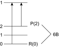

  

  Common upper states

  R(0) = 18147. 71, P(2) = 18, 146. 25

  R(0) − P(2) = 1. 46

  B″ = 1. 46∕6 = 0. 243 cm⁻¹

  B′ = B″ + a = 0. 157 cm⁻¹

• 4. Solve for r′, r″ from B′ and B″

Compare the values determined from rotational analysis with those listed in Herzberg [4]:

$$\displaystyle\begin{array}{rcl} B''_{e}& =& 0.2438,\alpha _{e} = 0.0017 \Rightarrow B''_{0} = 0.2438 - 0.0008 = 0.243 {}\\ B'_{e}& =& 0.158,\alpha _{e} = 0.003 \Rightarrow B'_{0} = 0.158 - 0.0015 \approx 0.157 {}\\ T_{e}& =& 18310.5,\ r''_{e} = 1.988\,\mathrm{\AA},r'_{e} = 2.47\,\mathrm{\AA} {}\\ \end{array}$$

2.7.4 Vibrational Analysis

Vibrational analysis can be used to determine ω _e  and x _e .

Band Origin Data

Absorption gives information on upper states, and emission gives information on lower states (Fig. 2.22).

Fig. 2.22

Absorption and emission between two potential wells

Deslandres Table

Tables of band origin values, known as Deslandres Tables, can be used via row analysis to get ω″ _e and $\omega _{e}x_{e}''$. With column analysis, information regarding ω _e ′ and $\omega _{e}x_{e}'$ can be retrieved (Fig. 2.23).

Fig. 2.23

Deslandres table with row and column analysis

Recall:

$$\displaystyle{\begin{array}{l} G(v) = \omega _{e}(v + 1/2) -\omega _{e}x_{e}(v + 1/2)^{2} \\ \left.\begin{array}{l} G(1) - G(0) = \omega _{e} - 2\omega _{e}x_{e} \\ G(2) - G(1) = \omega _{e} - 4\omega _{e}x_{e} \end{array} \right \rangle 2\omega _{e}x_{e} \end{array} }$$

2.8 Summary

Table 2.5 summarizes the analytical techniques covered thus far and the fundamental quantities that can be determined with them. Rotation is described by a rigid rotor, characterized by the rotational constant, B; however, non-rigid corrections due to vibrational (B _e , α _e ) and centrifugal (D _e , β _e ) distortion are often used to improve the model. Diatomic vibrations are usually described primarily as a harmonic oscillator (ω _e ) with a small, anharmonic correction ($\omega _{e}x_{e}$) that may become important at high vibrational energies.

Table 2.5 Analysis techniques and their related fundamental quantities

Absorption spectra, in general, can provide information on the upper state properties like D _e ′ (dissociation energy), T _e , and G(v′), as shown in Fig. 2.24. Emission spectra, conversely, provide information about the lower state, e.g., D _e ″ and G(v″), as shown in Fig. 2.25.

Fig. 2.24

Example potential wells and corresponding absorption spectrum for upper state propertiesTypical analyses for absorption include: 1. using band origin data to give G(v′) and hence G(v′ = 0). 2. using measured ν ₀ = T _e + G(v′ = 0) − G(v″ = 0) to find T _e . 3. using measured $\Delta$ to give D _e ′ via $\Delta + G(v'' = 0) = T_{e} + D_{e}'$.

Fig. 2.25

Potential curves and emission spectrum for lower-state propertiesTypical analyses for emission include: 1. using band origin data (Deslandres table) from fixed v′ to find G(v″). 2. using measured $\Delta$ and known T _e  and G(v′) to find D _e ″ via $D_{e}'' + \Delta = T_{e} + G(v')$.

2.9 Exercises

• 1. Which of the following molecules would show (a) a microwave (rotational) spectrum, and (b) an infrared (vibrational) spectrum: Cl₂, HCl, CO₂?

• 2. The rotational spectrum of¹H¹²⁷I shows equidistant lines 13.102 cm⁻¹ apart. What is the rotational constant, moment of inertia, and bond length for this molecule? What is the wavenumber of the $J = 8 \rightarrow J = 9$ transition? Find which transition gives rise to the most intense spectral line at 300 K. Calculate the angular velocity (in revolutions per second) of an HI molecule when in the J = 0 state and when in the J = 10 state.

• 3. Three consecutive lines in the rotational spectrum of H⁷⁹Br are observed at 84.544, 101.355, and 118.112 cm⁻¹. Assign the lines to their appropriate $J'' \rightarrow J'$ transitions, then deduce values for B and D, and hence evaluate the bond length and approximate vibrational frequency of the molecule.

• 4. The carbon monoxide molecule,¹²C¹⁶O, has a rotational constant, B _v , of 1.9226 cm⁻¹. Boltzmann’s equation gives the ratio of the population in rotational energy level J to the total number of molecules as shown below.

  $$\displaystyle{\frac{N_{J}} {N} = \frac{g_{J}} {Q_{\mathrm{rot}}}\exp \left (\frac{-E} {kT} \right )}$$

  The rotational degeneracy (i.e., the number of states with the same energy level), g _J , is given by 2J + 1, and the partition function Q _rot is given by $T/\theta _{\mathrm{rot}}$, where $\theta _{\mathrm{rot}} = B_{v}\left (\frac{hc} {k} \right )$.

  • (a) Find the rotational level that has the maximum population if T = 1000 K.

  • (b) Calculate the temperature which maximizes the population fraction N _J ∕N for the J value found in part (a).

  • (c) Plot N _J ∕N as a function of J for the two temperatures in (a) and (b).

• 5. The following are the line positions in wavenumber units of the fundamental and first overtone bands of BBr, with v″ = 0.

  Table 7

  • (a) Assign proper labels to all of the lines and calculate B _e , α, ω _e , $\omega _{e}x_{e}$.

  • (b) Estimate the centrifugal distortion coefficient D _e and use it to determine the centrifugal correction to the position of the P(3) line of the fundamental band. Assume D ₀ = D ₁ = D _e .

  • (c) Calculate the position of the P(1) and R(0) lines for the second overtone band of BBr.

• 6. The band origin of a transition in C₂ is observed at 19,378 cm⁻¹, while the rotational fine structure indicates that the rotational constants in excited and ground states are, respectively, B′ = 1. 7527 cm⁻¹ and B″ = 1. 6326 cm⁻¹; the centrifugal distortion parameters D′ and D″ are negligible. Determine the position of the bandhead, i.e. the branch, the value of J″, and the frequency of the transition. Which state has the larger equilibrium internuclear distance, r _e ?

• 7. The following lines (wavenumber units) were observed in the 4′–0″ band of the Lyman series of H₂ $[B^{1}\Sigma _{u}^{+} \leftarrow X^{1}\Sigma _{g}^{+}]$:

  $$\displaystyle{\begin{array}{cccc} 95,253.64&95,193.60&95,105.72&95,044.22 \\ 94,897.76&94,805.51&94,600.47&94,477.47 \\ 94,213.94&94,060.10&93,737.88&93,553.38 \\ 93,172.58&92,957.34&92,517.96&92,271.96 \\ 91,773.99& & & \\ \end{array} }$$

  Determine B′₄, B″₀, and the null gap.

  Helpful Hints:

  • (a) $^{1}\Sigma -^{1}\Sigma$ bands have only two branches: P and R.

  • (b) Since the H atom nuclear spin is 1/2, Fermi statistics apply and all J states are populated.

  • (c) It is often helpful in sorting out a spectrum to plot the line positions along the frequency axis.

  • (d) If a bandhead is apparent, you may wish to begin at the opposite end of the spectrum and try to find a pattern with constant second differences.

References

C.H. Townes, A.L. Schawlow, Microwave Spectroscopy (Dover Publications, New York, NY, 1975)
W.G. Vincenti, C.H. Kruger, Physical Gas Dynamics (Krieger Publishing Company, Malabar, FL, 1965)
M. Diem, Introduction to Modern Vibrational Spectroscopy (Wiley, New York, NY, 1993)
G. Herzberg, Molecular Spectra and Molecular Structure. Volume I. Spectra of Diatomic Molecules, 2nd edn. (Krieger Publishing Company, Malabar, FL, 1950)
C.N. Banwell, E.M. McCash, Fundamentals of Molecular Spectroscopy, 4th edn. (McGraw-Hill International (UK) Limited, London, 1994)
Author information
Authors and Affiliations
Rights and permissions
Copyright information
© 2016 Springer International Publishing Switzerland
About this chapter
Cite this chapter
Hanson, R.K., Spearrin, R.M., Goldenstein, C.S. (2016). Diatomic Molecular Spectra. In: Spectroscopy and Optical Diagnostics for Gases. Springer, Cham. https://doi.org/10.1007/978-3-319-23252-2_2
Download citation
DOI: https://doi.org/10.1007/978-3-319-23252-2_2
Publisher Name: Springer, Cham
Print ISBN: 978-3-319-23251-5
Online ISBN: 978-3-319-23252-2
eBook Packages: EngineeringEngineering (R0)