
Abstract
Dyadic data frequently occur in social sciences and numerous techniques have been developed for their analysis. The most prominent methods involve using regression, path, and structural equation models. The present contribution extends these approaches by considering Item Response Theory (IRT) Models. Two pivotal dyadic data analysis models, the Actor-Partner Interdependence Model (APIM) and the Common Fate Model (CFM), are built using the Multidimensional Random Coefficients Multinomial Logit Model (MRCMLM). This approach combines the advantages of dyadic data analysis with a model for discrete data, thus allowing for categorical items while drawing inferences based on the estimated true scores on an interval scale.
Access provided by Autonomous University of Puebla. Download conference paper PDF
Keywords
These keywords were added by machine and not by the authors. This process is experimental and the keywords may be updated as the learning algorithm improves.
Aims of This Contribution
This contribution presents a new approach to dyadic data analysis. It is organized as follows: After giving a short introduction to the basics of dyadic data (section “Dyadic Data”) and the core principles of their statistical analysis (section “Modeling Dyadic Data”), the fundamentals of a new approach based on multidimensional Item Response Models (mIRT; e.g. Reckase 2009) are worked out. This approach combines the specific requirements of dyadic data analysis (i.e., taking into account the dependencies within a dyad) with the advantages and flexibility of discrete probability models for categorical data. The principles of mIRT will be introduced in section “Item Response Models” and exemplified for two important dyadic data models, including computational details, in section “Worked Examples”.
Dyadic Data
Dyadic data originate from responses of individuals sharing a common context, like partner or parent-child relationships. Apart from such natural (or voluntary) linkage, a dyad can also be established by membership to a common context, like in an experimental design, where two previously unacquainted individuals are assigned to each other to work on a common task. We cannot assume the responses of linked observations (e.g., parent and child) to be mutually independent. We have to act on the assumption that systematic variation arises due to both, individual and relational characteristics. Four kinds of nonindependence may be discerned: compositional nonindependence (the dyad members are linked due to preexisting common characteristics), partner effects (characteristics or behaviors of one partner necessarily affects those of the other partner, e.g. when resources have to be shared), mutual influence (due to some sort of feedback loop), and common fate (both dyad members are affected by common circumstances, like sharing the household or consanguinity, for example).
Another crucial distinction has to be made with regard to the identifiability of the members of a dyad (pair) under consideration: While, for example, the roles of parent and child allow for a clear distinction of individuals, monozygotic twins may not be uniquely allocated unless auxiliary variables are taken into account (e.g., the elder vs. the younger sibling). Hence, we have to differentiate between dyadic data models for distinguishable and indistinguishable members.
Further, we have to consider whether information is gained at the individual or at the dyad level: A dyad member’s gender is usually a descriptor of the individual (except for studies deliberately focussing on same sex pairs, etc.), but the household income of a couple is identical for both members and therefore constitutes a dyad level variable. As a third category, we have to consider mixed variables, exhibiting variation on both the individual and the dyad level, like the respondents’ age.
A comprehensive overview of dyadic data, models, analyses, and numerous references to original sources can be found in Kenny, Kashy, and Cook (2006).
Modeling Dyadic Data
The term “model” refers in the context of dyadic data to a substantive perspective, i.e. how measurements from dyad members are hypothesized to relate to each other, and will not necessarily determine the statistical model to be used for parameter estimation. It might, therefore, be helpful to differentiate between “dyadic models,” focussing on substantive theory, and “statistical models.” This distinction is not always clear-cut, because some dyadic models may correspond closely to a certain statistical model.
Several models for dyadic data have been proposed so far, two of which are outlined in this section, as they are common in the literature, and they are further pursued in the analyses presented here. These are the Actor-Partner Interdependence Model (APIM) and the Common Fate Model (CFM).
The Actor-Partner Interdependence Model
Basically, the APIM (Kenny et al. 2006, ch. 7) constitutes a regression model involving an independent variable X and a dependent variable Y, both available for both members of a dyad (A and B). Hence, we deal with four variables (or constructs, if more than one item is involved), X A , X B , Y A , and Y B . The regressions of the Y -variables on the X-variables are separately modeled for each dyad member (called actor effects in the dyadic context, a YX and a′ YX in Fig. 1, top). In addition, each member’s X may affect the other member’s Y (called partner effects, p YX and p′ YX ). The magnitude of the partner effects relative to the actor effects expresses the extent of interdependence of dyad members. Furthermore, the two independent variables or constructs as well as the two dependent ones may exhibit a mutual relation (r X and r Y in Fig. 1, top).

Top: The Actor-Partner Interdependence Model (APIM). Bottom: The Common Fate Model (CFM). Notes: X: independent variable; Y: dependent variable; A, B: dyad members (e.g., actor/partner); a YX , a′ YX : actor effects; p YX , p′ YX : partner effects; r X , r Y : correlation of independent and dependent variables; r A , r B : correlation of X and Y for individuals A and B, respectively
If each of the four constructs involved (X A , X B , Y A , and Y B ) is a single random variable fulfilling certain scale and distributional assumptions, the coefficients could be determined by means of Ordinary Least Squares (OLS) regression or path analysis (a comprehensive instruction can be found in Kenny et al. (2006), for example). However, such an approach ignores the measurement errors of the observed variables and becomes increasingly cumbersome for dyadic models that are more complex than those considered here.
The nesting of individuals within dyads constitutes a hierarchical data structure, which facilitates the application of multilevel models (cf. Hox 2010; for their specific application to dyadic data, see Campbell & Kashy 2002 or Kenny et al. 2006, ch. 4). Alternatively, the coefficients could be estimated by means of Structural Equation Models (SEM; e.g., Bollen 1989). In particular the SEM-approach allows for a sophisticated and flexible modeling of the hypothesized relationships and provides a highly differentiated assessment of model fit.
The Common Fate Model
The CFM (Campbell 1958; Kenny et al. 2006, pp. 409–412) also considers the relationship of two variables (X and Y ) recorded for both members of a dyad (A and B). But instead of looking for mutual dyad members’ influence (the partner effects in the APIM), we focus on the correlation of X and Y, assuming that they constitute a common background (“fate,” hence the naming) for the individual expressions (X A , X B and Y A , Y B , respectively; cf. Fig. 1, bottom). As a special case, the CFM is particularly appropriate for designs, in which A and B express their assessment of a third person. This may be the case, for example, when both parents rate X and Y of their child, or a couple is asked to assess two characteristics X and Y of their marriage counselor.
The core principle of a CFM is that both X A and X B are affected by a latent variable X and, likewise, Y A and Y B can be traced back to a common latent variable Y. The latent correlation of X and Y reflects the substantial question of interest on the dyad-level. However, the two common fate constructs (X and Y ) may not account for the entire observed covariance of the manifest variables X A , X B , Y A , and Y B , as individual characteristics could have an impact as well. Such individual level effects are expressed by the correlation coefficients r A and r B as indicated at the bottom of Fig. 1.
Because of the assumption of latent factors that underlie the manifest variables, the SEM approach is the most suitable technique for CFMs. Besides, there are also methods available not involving latent constructs, but based on simple regression analysis (for an introduction, see Kenny et al. 2006, pp. 409–412). However, these should be considered outdated for the same reasons as in the APIM context.
Problem
SEM and Multi-Level Models prevail in current modeling approaches to dyadic data analysis. Either of these models requires certain scale and distributional prerequisites to be fulfilled—most prominently, in the standard case, interval scaled variables and (multivariate) normal distribution. Such assumptions are frequently made without hesitation. For example, Kenny et al. (2006) argue “Most scales developed and used in social science research are assumed to be measured on an interval scale” (p. 9), and “Throughout this book, we generally assume that outcome variables are measured at the interval level.” (Kenny et al. 2006, p. 10).
In many cases, constructs are captured with scales comprising a reasonable number of items to be endorsed through ordered categories or by responding in a simple yes/no style. If such a set of items has undergone thorough statistical analysis, a (possibly weighted) sum of scores might fulfill the aforementioned scale assumptions—at the price of restricting the number of applicable instruments to those having been scrutinized accordingly. Sometimes, a sum score is even computed without bothering about properties of the involved items—dimensionality and scale assumptions remain conjectures then.
Loeys and Molenberghs (2013) have proposed Generalized Linear Mixed Models for dyadic data analysis with categorical data and Loeys, Cook, De Smet, Wietzker, and Buysse (2014) used Generalized Estimating Equations. McMahon, Puget, and Tortu (2006) have shown how to model binary data employing a Multi-Level approach. Furthermore, Log-Linear Models may be applied as well (e.g., von Eye & Mun 2013; see Kenny et al. 2006, pp. 131–135 for their specific application to dyadic designs). Log-Linear Models also allow for testing interaction effects and the assessment of model fit. However, we will take a slightly different approach to categorical data here, using Item Response Theory (IRT; de Ayala 2009; van der Linden & Hambleton 1997; Lord 1980).
Item Response Models
Before delving into the details of how dyadic data models may be expressed through IRT models, a brief introduction to IRT reviews some basic characteristics. Generally, Item Response Models link manifest responses to latent response probabilities, expressed by model parameters, using a deliberately selected link function. Usually, the manifest responses are categorical, hence we deal with discrete probability models (an extension to quantitative responses has been developed by Müller 1987 but will not be further pursued here, as our intention is to model discrete data).
The Rasch Model and Some of Its Extensions
The most basic IRT model is the Rasch Model for dichotomous data (RM; Rasch 1960). It models the probability of a response x vi ∈ { 0, 1} of individual v (v = 1… n) to item i (i = 1… k) with two parameters, \(\theta _{v}\), quantifying the ability of person v, and δ i , quantifying the difficulty of item i. The link function is the logistic one. It yields the model equation
Note that a “positive” manifest response x vi = 1 may represent the solution of an item during an ability test or the endorsement of a statement during a personality assessment. Hence the traditional term “ability” may also be understood as “proneness” (in the sense of “disposedness”) to endorse a statement and “difficulty” as the “severity” or “particularity” of that statement.
The trace lines (or Item Characteristic Curves, ICC) of function (1) for selected δ i across an arbitrary range of \(\theta _{v}\) are parallel, which constitutes a distinct feature of the RM. The unweighted sum of scores x vi per row v and per column i are the sufficient statistics for the person ability parameters \(\theta _{v}\) and item difficulty parameters δ i , respectively. Either parameter vector, \(\boldsymbol{\theta }\) and \(\boldsymbol{\delta }\), can be estimated independently of the distribution of the other one, which caused Georg Rasch to develop his infamous principle of Specific Objectivity (SO; Rasch 1961 1966, 1977). One decisive advantage of SO is that it allows for a rigorous assessment of model fit (for an overview, see Glas & Verhelst 1995, for example). If the model holds, all items measure the same latent trait (unidimensionality assumption).
Numerous extensions have been developed. For ordered polytomous data, the Eq. (1) is adopted to model the thresholds between adjacent categories while retaining all advantageous features inherited from the RM. Applying various restrictions, this yields the Partial Credit Model (PCM; Masters 1982; Wright & Stone 1979) or the Rating Scale Model (RSM; Andrich 1978 1982; Wright and Masters 1982). If, on the other hand, substantial considerations allow for decomposing the items into a well-defined set of p basic (cognitive) operations or technical features, their difficulty can be quantified by means of the Linear Logistic Test Model (LLTM; Fischer 1973 1995). For that purpose, a k × p weight (or design) matrix A is set up based on substantial theory, linking each item parameter δ i to a hypothesized set of basic parameters \(\xi _{j}\) (j = 1… p; p ≤ k), which represent cognitive operations or technical features.
Furthermore, additional item-specific parameters have been introduced (at the expense of losing SO). These parameters relax the rather restrictive assumption of parallel trace lines, which may be difficult to attain, especially when analyzing large item pools. A discrimination parameter α i for each item (Birnbaum 1968) expresses the slope of an item’s ICC at its inflection point along the \(\theta\)-scale. It serves, roughly speaking, as a measure, of the degree to which the distinction (or “discrimination,” hence the naming) between two individuals is clear-cut by this item. Thus, the trace lines’ slopes are explicitly modelled rather than assumed parallel. In addition, an item specific guessing parameter may be employed, quantifying the probability of a positive response for arbitrary small values of the person ability parameters (technically, it defines the lower asymptote of an item’s ICC; Birnbaum 1968).
A third line of development introduced a third kind of parameter for designs, where individuals (represented by the person ability parameter \(\theta _{v}\)) respond to items (represented by the item difficulty parameters δ i ), and their responses are evaluated by raters. A rater’s (r) leniency may be quantified by means of a rater parameter ψ r (for details, see Linacre 1989).
Another important extension, crucial for modeling dyadic data, is introduced in the following section.
Multidimensional IRT Models
All IRT models sketched in section “The Rasch Model and Some of Its Extensions” share the assumption of unidimensionality, i.e. one single common latent trait being required for solving all items (or endorsing the respective statements) under consideration. In contrast, a set of items may also depend on several distinct latent traits, in fact in two ways: Either an item involves more than one trait (e.g., a math item embedded in a very complex instruction might require a certain amount of both language and math skills); such a case is referred to as within item multidimensionality. Or, one subset of items goes together with a latent trait \(\theta _{1}\) and a different subset of items with another latent trait \(\theta _{2}\); this case is called between item multidimensionality. In our application, we will refer to the latter case. The allocation of the i = 1… k items to \(\ell= 1\ldots m\) latent traits is specified in scoring matrix B = (b i ℓ ), which is—as A before—set up based on theoretical reasoning prior to parameter estimation. As a consequence, each individual’s ability profile (i.e., his or her location on each latent trait) is expressed through an individual’s ability vector \(\boldsymbol{\theta }_{v} = (\theta _{v\ell})\) of length m.
Now, combining such a person parameter decomposition with the item parameter decomposition sensu LLTM, as introduced in section “Item Response Models”, leads to the Multidimensional Random Coefficients Multinomial Logit Model (MRCMLM; Adams, Wilson, & Wang 1997; Adams & Wu 2007). It follows the logistic structure of Model (1), in which both parameters are replaced by a product of a weight matrix (i.e., the scoring matrix B for person parameters and the design matrix A for item parameters), and the respective item and person parameter vector. The model equation for an individual’s response vector \(\boldsymbol{x}_{vi}\) is
where
Parameter estimation is usually accomplished with the Marginal Maximum Likelihood technique (cf. Baker & Kim 2004). This technique requires a distributional assumption regarding the person parameters. It is common practice to choose the normal, yielding for the unidimensional case
Moreover, the MRCMLM allows for defining a correlational structure among the latent variables or regressing the latent variables onto each other and on a set of background variables Y, e.g., income or educational information. The latter leads to the so-called background model, which, in multivariate notation, shows as
with \(\boldsymbol{\gamma }\) expressing the regression weights of \(\boldsymbol{\theta }\) on Z and assuming \(\epsilon \sim N(0;\sigma _{\epsilon }^{2})\). Incorporating the background model (4) in the multivariate extension of (3) yields
with covariance matrix
This covariance matrix (more precisely, its estimates) will prove eminently useful for the task of expressing dyadic models in terms of item response models. These coefficients allow for expressing correlations among the latent constructs. Moreover, we may also estimate directed relationships among the latent constructs, allowing for a SEM-like modeling approach, yet on a solid Rasch foundation. The core idea is to obtain the correct SSCP matrix of all exogenous (“independend”) and endogenous (“dependent”) variables and to find the desired regression coefficients by means of the Two-Stage Least Squares (TSLS) estimation approach (Gebhardt, in prep; for a delightful description of the TSLS history see Stock & Trebbi, 2003).
Expressing Dyadic Data Models in Terms of Item Response Models
This section outlines the central principle of how dyadic data models may be formulated in terms of IRT Models. We will consider two important dyadic models, the APIM and the CFM. In the graphical representations, boxes represent manifest variables (which are, in our case, categorical) and ellipses represent latent constructs. The core principles of all models to be introduced are to (1) assume a separate latent trait for each of the “dyadic variables” (i.e., the X A , etc. in Fig. 1) and (2) model the postulated dyadic relationships in the latent domain, thus requiring a multidimensional model like the MRCMLM.
The APIM in Terms of an MRCMLM
Dyadic models as depicted in Fig. 1 assume relations among the X- and Y -measures of the dyad members A and B. While regression or path analysis assumes these constructs (i.e., X A , Y A , X B , and Y B ) to be manifest, we may also model each of them as a separate latent construct. Of course, this could be achieved with a SEM as well, but while the SEM (in its standard case) assumes the items’ responses to lie on an interval scale, we want to model truly categorical responses (like “agree”—“partially agree”—“disagree”) with a discrete probability model, such as the MRCMLM. Further, standard SEM applications use a linear link function of items and latent variables (although modifications for categorical variables have been developed as well, cf. Muthén 1984).
Each dyad (i.e., the pair A and B) forms a unit of observation v (usually a row in the data set). Hence the measures X A , Y A , X B , and Y B may be conceived as four latent dimensions of the dyad v and comply to one \(\theta _{\ell}\) of the MRCMLM as expressed in Eq. (2). We thus assert four latent constructs \(\theta _{1}\) to \(\theta _{4}\), constituting the four measures of interest (i.e., \(\theta _{1} = X_{A}\), and so on). Such a structure can be depicted as shown in Fig. 2. The double-headed arrows are based on the latent covariances [i.e., the elements of Matrix (6)] between the four constructs. Furthermore, the MRCMLM also allows for estimating a regression model of the latent constructs on the background variables [Eq. (4)] and on each other. The latter will be used to model the directed relationships as postulated in the APIM (and depicted by single-headed arrows in Fig. 1, top).

The basic structure of an APIM expressed as an MRCMLM
The CFM in Terms of an MRCMLM
Defining the CFM in terms of an MRCMLM is straightforward, as it already involves two latent constructs, \(\theta _{X}\) and \(\theta _{Y }\), representing the variables of interest (cf. Fig. 3). The latent factor \(\theta _{X}\) (representing X in Fig. 1, bottom) affects both dyad members’ observed values, X A and X B , and, therefore, represents the common background (fate) of A and B. The same applies to the other latent variable of interest, \(\theta _{Y }\). The latent correlation \(r_{\theta _{X}\theta _{Y }}\) is the central measure of interest. It expresses the association between \(\theta _{X}\) (the latent representation of X) and \(\theta _{Y }\) (the latent representation of Y ) after taking the relationship between the actors into account. It is indicated with a double headed solid arrow in Fig. 3.

The basic structure of a CFM expressed as an MRCMLM
Not all covariation of X and Y variables may be explained by the dyad level correlation \(r_{\theta _{X}\theta _{Y }}\), hence we further explore individual level correlations (termed r A and r B , respectively, indicated with dotted double headed arrows in Fig. 1). The calculation of these two coefficients requires additional reasoning. The latent factor \(\theta _{X}\) reflects the common self-perception regarding the trait under consideration. Analoguously, the latent factor \(\theta _{Y }\) reflects what is common in the other’s perception. However, these two latent factors could miss certain aspects of one’s self- or other’s perception. Such omitted information is collected in the residuals, which will be used to determine the individual correlation coefficients r A and r B (see section “The CFM Approach”).
Worked Examples
The proposed modeling approach shall be demonstrated in a psychological study focussing on selected personality traits of dyads of students and a parent. The question was whether the assessment of the respective other is influenced by the respective member’s self-assessment.
The Study Framework
The theoretical scope of the study allows for different questions to be addressed. We will apply both the APIM and the CFM approaches with one data set, the design of which is outlined below. The respective research questions will be explained in the specific context of the model.
Instrument
The Gießen-Test (GT; Beckmann, Bräahler, & Richter 1990) is a self-assessment consisting of the following six scales (German original terms in brackets):
-
social resonance (soziale Resonanz),
-
dominance (Dominanz),
-
control (Kontrolle),
-
prevailing mood (Grundstimmung),
-
responsiveness (Durchlässigkeit), and
-
social power (soziale Potenz).
The test consists of 40 bipolar items and respondents have to indicate their preference on a 7-point scale of the form
with (A) and (B) representing opposite characteristics of a person. According to the manual, the construction of the GT involved exploratory factor analyses, resulting in six items per scale. The GT is capable of dyadic assessment because it can be employed for both self and partner assessment. For that purpose, three different forms of the questionnaire are available. For the self-assessment, the questions are formulated as
The male/female partner assessment versions are worded
That way, four different versions exist and partnership assessment becomes feasible. Actor-self, Partner-self, Actor with respect to Partner, and Partner w.r.t Actor. Score sheets allow for comparing the four profiles. Note that there is also a dedicated partnership assessment version of the GT available, which uses only 5 out of the 6 scales. This version was not applied here, because it involves some indistinct scoring constants, not necessary for the present analysis.
Sample
The data set used for the present study has been simulated in a way that it reflects the characteristics of a smaller data set of psychology students. Hence, we will not draw substantial conclusions from the results obtained here. The students (first and third semester) were asked to fill out the questionnaire with respect to themselves and to a parent (preferably the mother). A total of 600 pairs has been simulated.
Method
Parameter estimation of the MRCMLM has been performed with the ConQuest 3.0 software package (Adams, Wu, & Wilson 2012). To avoid estimation problems, the responses were dichotomized at the midpoint of the response scale (left vs. right direction). The online version of the instrument used in the present study comprised only six response categories per item (leaving out the middle category), thus fostering dichotomization.
The APIM Approach
Regarding the six personality traits of the GT, one could conceive of the following situation: A student’s rating of the respective parent (\(\theta _{2}\)) depends on the parent’s status regarding that trait, reflected in their self ratings (\(\theta _{3}\)). Therefore, we expect a strong coefficient p′ YX (see Fig. 4). In addition, the student’s assessment might as well be influenced by his or her own Selbstbild, i.e. the way he or she perceives him- or herself with regard to the respective trait. For example, Sigmund Freud has keyed the term Projektion (projection), which describes, simply put, one’s proneness to perceive one’s own conflict-ridden, denied, or repressed emotions in others rather than in oneself (cf. Freud 1976; for more recent approaches see, for example, Baumeister, Dale, & Sommer 1998). Such a tendency would, if common, show in the regression coefficient a YX , i.e. the actor effect in APIM terminology: The lower the student’s self-rating, the higher his or her parent’s rating on that scale, hence a substantial negative regression coefficient would arise. Analoguously, such an effect might as well appear in the parent’s rating: His or her perception of the student (\(\theta _{4}\)) would primarily depend on the student’s trait, which should be expressed in the student’s self-rating (\(\theta _{1}\)), hence we expect a strong path p YX . But the parent’s Selbstbild might also influence this assessment—for example, because a parent might feel responsible for the offspring’s development. Hence, a non-zero path a′ YX might appear as well. Finally, we have to consider that parents and children are prone to be similar with respect to personality traits as measured by the GT, reflected by the correlation \(r_{\theta _{1}\theta _{3}}\) and which has to be corrected for.

Theoretical vs. empirical item characteristic curve (example plot for item 24). The dashed line represents the empirical ICC and the solid line the model derived ICC. Closeness of the two curves indicates a good model fit
We might therefore expect two strong (in terms of APIM) partner effects (p and p′) as well as possible (but presumably weaker) actor effects (a and a′), reflecting the raters’ involvement, like Projektion, for example. Moreover, a non-zero correlation of the two independent variables or the two dependent variables might occur as well. For each of the six GT scales, a separate APIM was estimated. For reasons of saving space, we will present only the results of the Social Resonance subscale.
Model Setup
The ConQuest 3.0 software accepts input via a command file. The ASCII-data file was named gt_res.dat. It comprised 25 columns (one ID and six items per subscale times four versions in the dyadic framework) with the responses coded numerically (1 to 6); missing data were coded with 9. Listing 1 shows the ConQuest command file for the APIM (a line by line explanation of these commands is given in Table 1 in Appendix “APIM Commands”).
Listing 1 ConQuest Command Script for the APIM (Note that each command has to be terminated with a semicolon)

These commands are stored in a file (named gt_res.cqc) and executed with the Run > Run all command from the menu bar (GUI version) or via submit gt_res.cqc; in the command line version.
Results
After submitting the command script to the program, a detailed output listing is available. The portions of this output relevant for building the APIM and assessing model fit will be described here.
Building the APIM from the Output One central part of the ConQuest output concerning the APIM is given in Listing 2. This section is produced by the structural commands in lines 15 and 16 of the command script.
In this output section we find the regression coefficients for the APIM, i.e., the single-headed arrows p YX , a YX , \(p'_{Y X}\), and \(a'_{Y X}\) according to Fig. 1, top. These coefficients can be found in the columns headed Gamma (lines 25–27 and 45–47 in Listing 2). Another essential part of the APIM, the correlation of the two independent variables, (r X in Fig. 1, top) can be found in the output section headed CONDITIONAL COVARIANCE/CORRELATION MATRIX (Listing 3).
Listing 2 Essential ConQuest Output for the APIM (Part 1a: Regression Coefficients)

Listing 3 Essential ConQuest Output for the APIM (Part 1b: Correlation Coefficients)

In this cut-out we find the estimated covariances (upper triangular matrix) and the correlations (lower triangular matrix) of the latent factors, i.e. the \(\hat{\sigma }_{\theta _{\ell}\theta _{\ell'}}^{2}\) and the \(\hat{r}_{\theta _{\ell}\theta _{\ell'}}\) for each pair \(\theta _{\ell}\) and \(\theta _{\ell'}\). Hence, we may now draw the final diagram of the APIM (Fig. 5).

The APIM approach of modeling other’s assessment taking the Selbstbild into account
Each parameter estimate is of course accompanied by its respective standard error, facilitating the application of the Wald statistic. Listing 4 presents the example output for the regression models of our example.
Listing 4 Essential ConQuest Output for the APIM (Part 1c: Regression Coefficients)

In order to obtain a test statistic for evaluating the null hypothesis that the parameter is zero, we have to divide the estimate by its standard error, yielding a standard normal variate. For example, to test the regression coefficient \(\gamma _{\theta _{ 2}\theta _{1}}\) for significance, we compute − 0. 135∕0. 051 = −2. 647, the absolute value of which is larger than the 95 % quantile of the standard normal. Hence the coefficient is significantly different from zero (as are all coefficients of this model). However, because the sample size of the present data set has been fixed arbitrarily to 600, such a test is not informative in our case.
Interpretation We find two distinct partner effects (p YX = 0. 463 and \(p'_{Y X} = 0.833\)). These results suggest effects of the personality of the target person (reflected in the students’ and parents’ self-description, \(\theta _{1}\) and \(\theta _{3}\)) on the respective other’s assessment. In contrast, the students’ actor effect is close to zero (a YX = 0. 031), hence there is no evidence for the assumption of Projektion (as regards students) as has been hypothesized. However, the parents’ actor effect is comparably large (a YX = 0. 602), which might be taken as an indicator for parental feelings of responsibility. The parameter \(r_{\theta _{2}\theta _{4}} = 0.2\) shows that the ratings of the respective other are nearly uncorrelated, when taking the actor and partner effects into consideration.
Assessment of Model Fit As was noted above, the MRCMLM also allows for a multifaceted assessment of model fit. First of all, ConQuest supports the item mean square statistics Outfit (Unweighted Mean Square Statistic) and Infit (Weighted Mean Square Statistic). Basically, these are measures of discrepancy between observed and expected responses. Model fit is indicated by values close to one for either statistic (for details see Wright & Stone 1979). Listing 8 in Appendix “APIM Item Fit Indices” presents the model fit segment of the output. Generally, item fit is not convincing in our case, as many of the indexes lie outside the given confidence intervals (and, correspondingly, have t-values larger than 2).
Furthermore, the parameter estimates allow for expressing a reliability coefficient comparable to the one from classical test theory (cf. ConQuest manual, Wu, Adams, Wilson, & Haldane, 2007, p. 160). Listing 5 shows the original program output regarding this “Andrich-Reliability.” It seems that all four latent constructs have low reliability, possibly a consequence of data dichotomization. Due to the artificial nature of the data, we will refrain from further interpretating this result.
Listing 5 Essential ConQuest Output for the APIM (Part 3: Scale Reliability)

A measure of item fit is based on the comparison of observed and model derived ICC. The program delivers one such plot per item, one of which is shown in Fig. 6.

The final APIM based on the MRCMLM
The horizontal axis shows the latent trait (\(\theta\)) in the interval [−4, +4] (covering the most frequently obtained values). The solid line is the expected probability of a positive response to item i, i.e. P(X vi = 1) according to Eq. (2) for \(\theta _{v} \in [-4,+4]\), and the dotted line is the relative frequency of X vi = 1 for all observed score groups (also called the empirical ICC). The closeness of the two lines is an expression of model fit.
The CFM Approach
We now discuss the correlation of the self-descriptions and the descriptions of the respective other more generally. We could assume that the complex processes within the family (here considering the dyad of two family members only) form the common background for developing a personality (\(\theta _{1}\) and \(\theta _{3}\)) on the one hand and also establishing a common background for the perception of the family member (\(\theta _{2}\) and \(\theta _{4}\)), on the other hand. Of course, individual components not captured by the correlation on the dyadic level may play an important role as well. These are expressed by the correlation coefficients of the residuals as described in section “The CFM in Terms of an MRCMLM”. The MRCMLM directly delivers an estimation of the dyadic correlation coefficient with the (standardized) entries of the covariance matrix (6), while the individual level correlation coefficients require a little bit of craftsmanship.
Model Setup
The command script for the MRCMLM formulation of the CFM is similar to the previous script. However, the assignment of items to latent factors differs as we now just use two latent factors for all self-description items on the one hand and the items expressing the partners’ assessments, on the other hand (lines 5–8 in Listing 6).
Listing 6 ConQuest Command Script for the CFM

In line 14 of Command Script 6 the residuals are written into a file named resid.txt. These residuals are used to compute the individual level correlation coefficients r A and r B . In the present example, students and parents have responded to the same items. In order to take this mapping into account, we compute the correlation coefficients of the associated residuals (i.e., item 1 of student/self with item 1 of student \(\rightarrow\) parent, etc.). The items within one block (e.g., all items regarding the self-rating of the student) are assumed to measure unidimensional. As a consequence, the residuals of each block represent the individual information not covered by the latent scales \(\theta _{X}\) and \(\theta _{Y }\). We therefore compute the average of the correlation coefficients (cf. Monin & Oppenheimer 2005) across items per individual in order to obtain the desired coefficients r A and r B (cf. ellipses in Fig. 7; for technical details see Appendix “Extracting the Individual Level Correlation Coefficients”).

Structure of the correlation matrix of the residuals
Results
The essential output providing the CFM coefficients is given in Listing 7, where we find the estimated covariance (upper triangular matrix) and the correlation coefficient (lower triangular matrix) of the latent factors, i.e. the \(\hat{\sigma }_{\theta _{\ell}\theta _{\ell'}}^{2}\) and the \(\hat{r}_{\theta _{\ell}\theta _{\ell'}}\) for each pair \(\theta _{\ell}\) and \(\theta _{\ell'}\). The bottom line contains the estimated variances of each latent variable, \(\hat{\sigma }_{\theta _{\ell}}^{2}\), with the corresponding standard errors in brackets.
In this output we find that \(\hat{r}_{\theta _{1}\theta _{2}} = 0.501\), indicating a medium sized correlation of the two latent constructs. Again, we may apply the Wald statistic to test whether this coefficient differs significantly from zero.
Listing 7 Essential ConQuest Output for the CFM (Part 1: Latent Correlation)

Next, we have to extract the residual correlations within individuals (student and parent, indicated by dashed double headed arrows in Fig. 7). For that purpose we have to evaluate the residuals stored in the external file, as has been done in line 14 of Listing 6. The necessary steps are explained in Listing 9 in Appendix “Extracting the Individual Level Correlation Coefficients”, resulting in \(r_{XY }^{(Student)} = -0.017\) and \(r_{XY }^{(Parent)} = -0.010\).
Interpretation Interestingly, we find for Social Resonance only a dyadic correlation, while the two individual level correlation coefficients are in fact zero. From this, we could conclude that the common factors reflecting familial bonds seem to predominantly explain the agreement of self-description and other’s assessment. Because of the nature of the data used for this analysis, we will again refrain from an in-depth interpretation of this evidence.
Assessment of Model Fit Model fit may be assessed in the same way as in the APIM. The item fit indices (Listing 10 in the Appendix) indicate that a few items do not fit and thus require further investigation. The Scale Reliability Coefficient for the self-rating latent scale was 0. 401 and the value for the other’s rating was 0. 512. Both indicate slightly better fit than the scales constructed in the APIM. This could be an effect of scale length, as each latent factor comprises 12 items in the CFM, while there were only six items per scale in the APIM.
The ICC analysis would involve inspection of one plot per item, which is omitted here. Over all, acceptable model fit seems within range.
Discussion
The present contribution has demonstrated how two models of dyadic data analysis, the APIM and the CFM, can be cast in terms of a multidimensional Rasch Model, the MRCMLM. These two approaches have been conducted, yet many more could be conceived of. The common denominator is that the constructs of interest are not measured directly but rather with a set of variables each. These manifest variables are—as is often the case in social research—dichotomous or ordered categorical. Using the MRCMLM, a discrete probability model, we estimate a latent factor for each such construct. The relationships of these latent factors are then modeled in the latent domain.
Of course, one could argue that the SEM approach is readily applicable to ordinal or (ordered) categorical data as well by setting up an appropriate covariance matrix, using tetra- or polychorical correlation coefficient estimates. This argument definitely applies, but we must bear in mind that this extra step requires larger samples than the standard product-moment correlation coefficient for interval scaled variables (at least if standard maximum likelihood estimation is applied, which is usually the case; cf. Choi, Peters, & Mueller 2010). Alternatively, one may regard the category codings as valid quantifications of response categories assumed to be evenly spaced, hence assuming to work with coarsely categorized interval scaled variables in the sense of Bollen and Barb (1981). However, distributional issues may still arise then. If so, a Weighted ML Estimation Method is available, involving the estimation of the fourth moments. These require, for k items, the computation of a covariance matrix consisting of \((k^{4} + 2k^{3} + k^{2})/4\) elements. Such a matrix would require a large number of observations to attain estimates with sufficient precision. Note that this argument also applies to data measured on an interval scale, when the distributional assumptions are unclear. Hence, we may apply SEM by all means to (ordered) categorical data. However, the approach presented here treats such data in a much more natural manner, as it deliberately models the way, a latent response propensity \(\theta\) is transformed into a response probability \(P\left (x_{vi}\vert (\cdot )\right )\). One advantage of this approach is that departures from the postulated link function can be detected, as has been exemplified in Fig. 6.
The MRCMLM applies the marginal maximum likelihood parameter estimation method, which assumes the person parameters to follow a certain distribution, usually the normal [cf. Eq. (5)]. Such an assumption may not necessarily hold (cf. Blanca, Arnau, López-Montiel, Bono, & Bendayan 2013; Micceri 1989), which might introduce an estimation bias. However, this assumption is a consequence of the applied estimation method, not of the model itself. Rasch Models not including a background structure as introduced in Eq. (4) support the conditional parameter estimation technique (Andersen 1970 1980), even in the multidimensional case (Andersen 1977). The CML estimation method conditions on the sufficient statistics of the incidental (in the sense of Neyman & Scott 1948) parameters and thus makes no distributional assumptions at all (for a comparison of MML and CML, see Adams & Wu, 2007, pp. 68–69). Moreover, the CML approach facilitates a model test (Andersen 1973), allowing for a rigid assessment of model fit.
When applying the APIM, researchers may be particularly interested in estimating two ratio parameters k = p∕a and \(k' = p'/a'\) with p/p′ representing the respective partner effects and a/a′ representing the according actor effects (cf. Fig. 4). The ratios k and k′ can be used to describe specific patterns in the APIM (e.g., k = 1 refers to a couple pattern, k = −1 refers to a contrast pattern, and k = 0 refers to an actor-only pattern). Kenny and Ledermann (2010) proposed a phantom variable approach to estimate k along with its standard error in the SEM context, thus allowing for a significance test of k as well. A merely descriptive value of k may be obtained with the estimated coefficients γ from the standard MRCMLM output.
One valuable option has not been incorporated in the presented examples: Each model could be enhanced with a background population model, thus controlling the latent variables for background variables (like age or socio-economic information, for example). Further extensions would consider non-distinguishable dyads or more complex designs (like the One-with-Many Design, taking more than two individuals into account).
While our examples have only dealt with dichotomous data, the full bandwith of IRT models for polytomous categorical data is readily available. Furthermore, one could drop the assumption of parallel trace lines and include a discrimination parameter in the model equation, thus explicitly capturing differing item characteristics within the items of a scale as well. Such extensions would allow for a wider range of items to be used.
Altogether, the presented approach provides a powerful framework for the complex requirements of dyadic data modeling, taking both scale and distributional requirements into account.
References
Adams, R. J., Wilson, M., & Wang, W.-C. (1997). The multidimensional random coefficients multinomial logit model. Applied Psychological Measurement, 21, 1–23.
Adams, R. J., & Wu, M. L. (2007). The mixed-coefficients multinomial logit model: A generalized form of the rasch model. In M. von Davier & C. H. Carstensen (Eds.), Multivariate and mixture distribution Rasch models. Extensions and applications (pp. 57–75). New York, NY: Springer.
Adams, R. J., Wu, M. L., & Wilson, M. (2012). Conquest 3.0 [Computer software]. Melbourne: Australian Council for Educational Research (ACER).
Andersen, E. B. (1970). Asymptotic properties of conditional maximum likelihood estimators. Journal of the Royal Statistical Society, Series B, 32, 283–301.
Andersen, E. B. (1973). A goodness of fit test for the Rasch model. Psychometrika, 38, 123–140.
Andersen, E. B. (1977). Sufficient statistics and latent trait models. Psychometrika, 42, 69–81.
Andersen, E. B. (1980). Discrete statistical models with social science applications. Amsterdam: North-Holland.
Andrich, D. (1978). A rating formulation for ordered response categories. Psychometrika, 43, 561–573.
Andrich, D. (1982). An extension of the Rasch Model for ratings providing both location and dispersion parameters. Psychometrika, 47, 105–113.
Baker, F. B., & Kim, S.-H. (2004). Item response theory. Parameter estimation techniques. New York, NY: Marcel Dekker.
Baumeister, R. R., Dale, K., & Sommer, K. L. (1998). Freudian defense mechanisms and empirical findings in modern social psychology: Reaction formation, projection, displacement, undoing, isolation, sublimation, and denial. Journal of Personality, 66, 1081–1124.
Beckmann, D., Bräahler, E., & Richter, H.-E. (1990). Der Gießen-Test (GT). Ein Test für Individual- uind Gruppendiagnostik [The Gießen test (GT). A test for the assessment of individuals and groups] (4th ed.). Bern: Hans Huber.
Birnbaum, A. (1968). Some latent trait models and their use in inferring an examinee’s ability. In F. M. Lord & M. E. Novick (Eds.), Statistical theories of mental test scores with contributions by A. Birnbaum (pp. 395–479). Reading, MA: Addison-Wesley.
Blanca, M. J., Arnau, J., López-Montiel, D., Bono, R., & Bendayan, R. (2013). Skewness and kurtosis in real data samples. Methodology, 9, 78–84.
Bollen, K. A. (1989). Structural equations with latent variables. Hoboken, NJ: Wiley.
Bollen, K. A., & Barb, K. H. (1981). Pearson’s r and coarsely categorized measures. American Sociological Review, 46, 232–239.
Campbell, D. T. (1958). Common fate, similarity, and other indices of the status of aggregates of persons as social entities. Behavioral Science, 3, 14–25.
Campbell, L., & Kashy, D. A. (2002). Estimating actor, partner, and interaction effects for dyadic data using PROC MIXED and HLM: A guided tour. Personal Relationship, 9, 327–342.
Choi, J., Peters, M., & Mueller, R. O. (2010). Correlational analysis of ordinal data: From Pearson’s r to Bayesian polychoric correlation. Asia Pacific Educational Review, 11, 459–466.
Gebhardt, E. C. (in preparation). Latent Path Models within an IRT Framework. Unpublished doctoral dissertation, University of Melbourne, Melbourne, Australia.
de Ayala, R. J. (2009). The theory and practice of item response theory. New York, NY: Guilford.
Fischer, G. H. (1973). The linear logistic test model as an instrument in educational research. Acta Psychologica, 37, 359–374.
Fischer, G. H. (1995). The linear logistic test model. In G. H. Fischer & I. W. Molenaar (Eds.), Rasch models. Foundations, recent developments, and applications (pp. 131–155). New York, NY: Springer.
Freud, S. (1976). In J. Strachey (Ed.), The complete psychological works of Sigmund Freud (The standard edition). New York, NY: W. W. Norton & Company.
Glas, C. A. W., & Verhelst, N. D. (1995). Testing the Rasch model. In G. H. Fischer & I. W. Molenaar (Eds.), Rasch models. Foundations, recent developments, and applications (pp. 69–95). New York, NY: Springer.
Hox, J. J. (2010). Multilevel analysis. Techniques and applications (2nd ed.). New York, NY/Hove: Routledge.
Kenny, D. A., Kashy, D. A., & Cook, W. L. (2006). Dyadic data analysis. New York, NY: Guilford.
Kenny, D. A., & Ledermann, T. (2010). Detecting, measuring, and testing dyadic patterns in the actor-partner interdependence model. Journal of Family Psychology, 24, 359–366.
Linacre, J. M. (1989). Multi-facet Rasch measurement. Chicago, IL: Mesa Press.
Loeys, T., Cook, W., De Smet, O., Wietzker, A., & Buysse, A. (2014). The actor-partner interdependence model for categorical dyadic data: A user-friendly guide to GEE. Personal Relationships, 21, 225–241.
Loeys, T., & Molenberghs, G. (2013). Modeling actor and partner effects in dyadic data when outcomes are categorical. Psychological Methods, 18, 220–236.
Lord, F. M. (1980). Applications of item response theory to practical testing problems. Hillsdale, NJ: Lawrence Erlbaum Associates.
Masters, G. N. (1982). A Rasch model for partial credit scoring. Psychometrika, 47, 149–174.
McMahon, J. M., Puget, E. R., & Tortu, S. (2006). A guide for multilevel modeling of dyadic data with binary outcomes using SAS PROC NLMIXED. Computational Statistics & Data Analysis, 50, 3663–3680.
Micceri, T. (1989). The unicorn, the normal curve, and other improbable creatures. Psychological Bulletin, 105, 156–166.
Monin, B., & Oppenheimer, D. M. (2005). Correlated averages vs. averaged correlations: Demonstrating the warm glow heuristic beyond aggregations. Social Cognition, 23, 257–278.
Müller, H. (1987). A rasch model for continuous ratings. Psychometrika, 52, 165–181.
Muthén, B. (1984). A general structural equation model with dichotomous, ordered categorical and continuous latent variable indicators. Psychometrika, 49, 115–132.
Neyman, J., & Scott, E. L. (1948). Consistent estimates based on partially consistent observations. Econometrica, 16, 1–32.
R Core Team. (2014). R: A language and environment for statistical computing [Computer software manual], Vienna, Austria. Retrieved from http://www.R-project.org
Rasch, G. (1960). Probabilistic models for some intelligence and attainment tests. Copenhagen: Danmarks Pædagogiske Institut.
Rasch, G. (1961). On general laws and the meaning of measurement in psychology. Copenhagen: The Danish Institute of Educational Research.
Rasch, G. (1977). On specific objectivity: an attempt at formalizing the request for generality and validity of scientific statements. Danish Yearbook of Philosophy, 14, 58–93.
Rasch, G. An informal report on the present state of a theory of objectivity in comparisons. In Proceedings of the NUFFIC International Summer Session in Science at “Het Oude Hof”, The Hague, 14–28, July, 1966. Retrieved July 22, 2015, from http://www.rasch.org/memo1966.pdf.
Reckase, M. D. (2009). Multidimensional item response theory. New York, NY: Springer.
Stock, J. H., & Trebbi, F. (2003). Who invented instrumental variable regression? Journal of Economic Perspectives, 17, 177–194.
van der Linden, W. J., & Hambleton, R. K. (Eds.). (1997). Handbook of modern item response theory. New York, NY: Springer.
von Eye, A., & Mun, E.-Y. (2013). Log-linear modeling: Concepts, interpretation, and application. Hoboken, NJ: Wiley.
Wright, B. D., & Masters, G. N. (1982). Rating scale analysis. Chicago, IL: Mesa Press.
Wright, B. D., & Stone, M. H. (1979). Best test design. Chicago, IL: Mesa Press.
Wu, M. L., Adams, R. J., Wilson, M. R., & Haldane, S. A. (2007). ACER ConQuest. Generalised item response modelling software. Melbourne: ACER Press.
Acknowledgements
I am indebted to Paul Czech for his assistance during data acquisition of the students’ sample.
Author information
Authors and Affiliations
Corresponding author
Editor information
Editors and Affiliations
Appendices
Technical Appendix: APIM Commands
APIM Item Fit Indices
Listing 8 Item Fit Indices for the APIM

- item::
-
Item number and label; as no label has been provided, the item number is repeated.
- ESTIMATE::
-
Item parameter estimate; in the dichotomous case, this is the item difficulty parameter [δ i according to Eq. (1)]. To identify a latent scale, one item per latent dimension is fixed (indicated by an asterisk). By default, ConQuest sets the sum of the item parameters per latent dimension to zero (e.g.: − 1. 452 + 0. 688 + 0. 137 + 0. 147 + (−0. 124) +0.604 = 0). This could be overridden with the command set constraint=cases, causing the mean of the latent variable to be fixed at zero.
- ERROR::
-
Standard error of item difficulty parameter.
- MNSQ::
-
Outfit (UNWEIGHTED FIT) and Infit (WEIGHTED FIT) Index.
- CI::
-
The 95 % confidence interval for the expected value (i.e., 1) of Infit and Outfit.
- T::
-
The t-statistic for the null hypothesis that the Outfit and Infit Index is 1. Values larger than 2 may be considered significant at the 95 % level (corresponds to MNSQ outside the CI).
Extracting the Individual Level Correlation Coefficients
To obtain the individual level correlation coefficients, we use the residuals stored in resid.txt. This file contains 600 lines and 25 columns. The first column is a numerical dyad identifier, followed by four groups of six columns each, comprising the residuals to the respective six items of student/self, student w.r.t parent, parent/self and parent w.r.t student. Any multi-purpose statistics software can be used to obtain the individual level correlation coefficients. We will resort to the R software (R Core Team 2014) for it is freely available (open source) and easy to use. The following script will perform the required steps:
Listing 9 R Script for Computing the CFM Individual Level Correlation Coefficients

The ten statements of Listing 9 perform the following operations:
-
In line 1 of the script, we read the content of the file resid.txt and store it in a data.frame named d0.
-
Then (line 2) we transform the missing values (ConQuest codes them with -99 by default) to the R missing indicator NA.
-
In lines 3–6, the columns obtain more informative variable names (the output file contains no header, therefore, R uses the generic names V1 to V25 by default). This step is merely cosmetic and may as well be omitted.
-
Next (line 8), we compute the 25 × 25 correlation matrix of all residuals (omitting the id variable stored in column 1). A schematic view of this matrix is given in Fig. 8.
Fig. 8 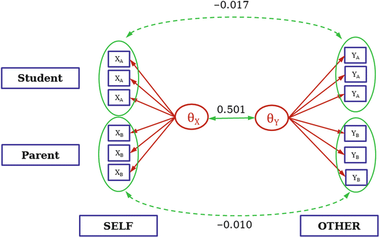
The final CFM
-
In line 10, we cut out blocks of correlation coefficients of the residuals of the students’ self-description items with the columns covering the residuals of the students’ assessments of the respective parents (rows 1–6/columns 7–12; grey shaded area termed rA in Fig. 8).
-
Analoguously, in line 11, we cut out the correlation coefficients of the residuals of the parents’ self-assessment items with the residuals of the items covering the parents’ assessments of the respective students (rows 13–18/columns 19–24; grey shaded area termed rB in Fig. 8).
-
In lines 13 and 14 we prepare two functions, transforming a correlation coefficient to a Fisher’s Z-value (r2z) and backtransforming the latter into a correlation coefficient again (z2r). These functions could easily be enhanced to detect invalid input and issue a corresponding message.
-
Finally (lines 16 and 17), we apply the Z-transformation to the two matrix parts, compute the mean and backtransform it to a valid correlation coefficient.

With these steps, we dispose of all required information to draw the complete CFM, depicted in Fig. 7.
CFM Item Fit Indices
Listing 10 Item Fit Indices for the CFM

For an explanation of the column headings see Appendix “APIM Item Fit Indices”.
Rights and permissions
Copyright information
© 2015 Springer International Publishing Switzerland
About this paper
Cite this paper
Alexandrowicz, R.W. (2015). Analyzing Dyadic Data with IRT Models. In: Stemmler, M., von Eye, A., Wiedermann, W. (eds) Dependent Data in Social Sciences Research. Springer Proceedings in Mathematics & Statistics, vol 145. Springer, Cham. https://doi.org/10.1007/978-3-319-20585-4_8
Download citation
DOI: https://doi.org/10.1007/978-3-319-20585-4_8
Publisher Name: Springer, Cham
Print ISBN: 978-3-319-20584-7
Online ISBN: 978-3-319-20585-4
eBook Packages: Mathematics and StatisticsMathematics and Statistics (R0)