
Abstract
The long-standing decentralized optimal control problem posed by Witsenhausen is analyzed and the underlying modeling issues are discussed. The strong connection to communication theory is highlighted. Informational aspects are emphasized and it is shown that, to some extent, Witsenhausen’s decentralized optimal control problem is somewhat contrived.
Access provided by Autonomous University of Puebla. Download conference paper PDF
Keywords
1 Introduction
Informational issues in decentralized control are discussed. In this regard, Witsenhausen’s problem [1] is the simplest decentralized optimal control problem. Indeed, the “simple” LQG control problem posed by Witsenhausen in his seminal paper made a great splash when it first appeared in 1968 because the optimal linear strategy is not optimal. This is caused by the nonclassical information pattern. Since then numerous attempts have been made in the intervening 45 years to obtain a better estimate of the minimal cost. A special session devoted to the Witsenhausen problem was held at the 2008 CDC and this stimulated renewed interest in the subject matter. Recently numerous additional papers on Witsenhausen’s counterexample have appeared, and this problem was also extensively addressed in the most recent CDCs [2–6]. There is a fascination with Witsenhausen’s counterexample in control circles and for good reason: It touches on the dual control issue where one needs to strike a balance between exploration and exploitation—this, exclusively due to the information pattern, which is non-nested. However, the objective of this article is not to survey the field, nor is it to further slightly improve the estimate of the minimal cost—the current best estimate of the minimal cost for the “canonical” problem parameters currently stands at 0.1670790. The objective is to gain an understanding of the underlying engineering or physical problem that Witsenhausen’s mathematical model is addressing. In this respect, the coupled communications and control aspects of Witsenhausen’s problem are discussed and the attendant informational issues are carefully examined. Also, our aim is to gain physical insight into a range of methods for obtaining suboptimal solutions and, by doing so, dispel some of Witsenhausen’s counterexample mystique. The strong connection to communication theory is emphasized and the informational aspects of the problem are highlighted. The latter seem to direct one to the conclusion that Witsenhausen’s decentralized optimal control problem is to some extent contrived.
The paper is organized as follows. In Sect. 2 Witsenhausen’s problem is carefully stated. In Sect. 3 the communications aspect of Witsenhausen’s decentralized LQG optimal control problem are analyzed and the connection to detection theory is elucidated in Appendix A. The special case where the “receiver’s” noise floor is high is analyzed in Sect. 4 and the optimal modulation and detection scheme is shown to be linear. Concluding remarks are made in Sect. 5.
2 Witsenhausen’s Problem Statement
In Witsenhausen’s paper [1] the following decentralized LQG optimal control problem is considered.
-
1.
Dynamics: The discrete-time dynamics are linear and scalar, and the planning horizon is N = 2. There are two “players,” Player 1 and Player 2. Player 1 acts at decision time k = 0 and his input is u 0:
$$\displaystyle\begin{array}{rcl} x_{1}& =& x_{0} + u_{0},\ x_{0} \sim \mathcal{N}(0,\sigma _{0}^{2}). {}\end{array}$$(1)Player 2 acts at decision time k = 1 and his input is u 1:
$$\displaystyle\begin{array}{rcl} x_{2}& =& x_{1} - u_{1}. {}\end{array}$$(2) -
2.
Information: The information of Player 1 at his decision time k = 0 is the initial state x 0. The information available to Player 2 at his decision time k = 1 is a noise corrupted measurement of the state at time k = 1,
$$\displaystyle\begin{array}{rcl} z_{1} = x_{1} + v_{1},\ \ v_{1} \sim \mathcal{N}(0,\sigma ^{2}).& & {}\end{array}$$(3)Thus, the initial state x 0 is the private information of Player 1 which is not shared with Player 2. Player 1 has perfect information at his decision time k = 0, whereas Player 2 which acts at time k = 1 has access to the noise corrupted measurement z 1 of the state x 1. Thus, at his decision time k = 1, Player 2 has imperfect information on the state x 1. In addition, Player 2 does not know the control u 0 of Player 1.
However, note that in [1], and in Eq. (1), it is also stated that the initial state x 0 is a random variable which is Gaussian distributed. This important point will be further discussed in the sequel.
-
3.
Strategy: The so far specified information pattern mandates that the strategy of Player 1 is
$$\displaystyle\begin{array}{rcl} u_{0} =\gamma _{0}(x_{0})& & {}\end{array}$$(4)and the strategy of Player 2 is
$$\displaystyle\begin{array}{rcl} u_{1} =\gamma _{1}(z_{1}).& & {}\end{array}$$(5) -
4.
Payoff: The cost function, which both players strive to minimize, is
$$\displaystyle\begin{array}{rcl} J(u_{0},u_{1};x_{0}) = K^{2}u_{ 0}^{2} + x_{ 2}^{2}.& & {}\end{array}$$(6)Player 1, who has perfect state information, has a penalty K 2 on his control effort, whereas the control effort of Player 2, whose states’ measurements are corrupted by noise, is free. Both players want the terminal state x 2 to be “small” while at the same time, the control effort, exclusively expanded by Player 1, also to be “small.” Evidently, Player 2 could effortlessly make the terminal state x 2 ≈ 0, if only he knew the state x 1 with a high degree of precision.
As far as Player 1 is concerned, the random variable in the problem statement is the measurement error v 1 of Player 2. As far as Player 2 is concerned, the random variables in the problem statement are the initial state x 0 and his measurement error v 1. The players are interested in the expectation of the cost function (6), which requires Player 1 to take the expectation on the random variable v 1 and Player 2 takes the expectation on the random variables v 1 and x 0. Since the Players 1 and 2 have private information, x 0 and z 1, respectively, their expected costs will be conditional on their private information. This brings us into the realm of nonzero-sum games.
Witsenhausen’s decentralized control problem is schematically illustrated in Fig. 1.
Fig. 1 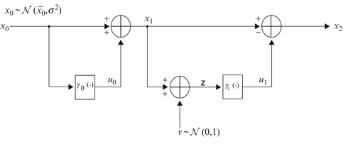
Witsenhausen’s decentralized control problem
In Fig. 1 we have allowed for a more general initial state specification,
$$\displaystyle\begin{array}{rcl} x_{0} \sim \mathcal{N}(\overline{x}_{0},\sigma _{0}^{2})& & {}\end{array}$$(7)and, without loss of generality, have set the parameter σ = 1; if σ = 0, the optimization problem is trivial—obviously, the optimal controls are \(u_{0}^{{\ast}} = 0\) and \(u_{1}^{{\ast}} = z_{1}\). The other extreme case where σ → ∞ will be addressed in Sect. 4. Thus, the problem parameters are K and σ 0.

2.1 Initial State Information
In Witsenhausen’s paper it is stated that the initial state x 0 is random, Gaussian distributed, and its statistics are specified according to Eq. (1), namely,
The informational aspect of the specification of the initial state’s statistics merits special attention.
In Witsenhausen’s paper [1], attention is confined to the special case where the statistic \(\overline{x}_{0} = 0\). It stands to reason that the consideration of a more general initial state is warranted, s.t. its statistics are specified by Eq. (7)—see also Fig. 1. Indeed, including in the problem statement the initial state’s statistics immediately begs the question: why not allow for a more generic form of the initial state information, as specified in Eq. (7), whereupon the issue of who knows what, when, is immediately brought up; exclusively considering the special case where the initial state’s statistic \(\overline{x}_{0} = 0\) tends to hide the importance of the \(\overline{x}_{0}\) information. This brings to the forefront the question of whether Player 1, or Player 2, or both players are privy to the \(\overline{x}_{0}\) information.
Consider Eqs. (7) or (1). This can be construed to mean that at time k = 0, Player 2 took a measurement of the initial state x 0 so that at his decision time k = 1, Player 2, in addition to the measurement z 1, also has imperfect information about the state x 0. Thus, the strategy (5) of Player 2 should in fact be replaced by the strategy
Whether or not Player 1 is informed on the initial state’s measurement taken by Player 2 is an important question. If indeed the measurement information \(\overline{x}_{0}\) is shared with Player 1 then his strategy (4) should be replaced by the strategy
Clearly, should at time k = 0 the information on the measurement \(\overline{x}_{0}\) of Player 2 be shared with Player 1, Witsenhausen’s control problem would be somewhat less decentralized than it appears to be at first glance.
Alternatively, one might argue that the specifications in Eqs. (1) or (7) mean that although it is so that at his decision time k = 0, Player 1 has perfect state information, he might be aware of the fact that the initial state x 0 presented to him at time k = 0 will actually be drawn from the distributions (1) or (7). This is critical information if a degree of information sharing among the players before the kickoff of this seemingly decentralized control problem is in fact allowed, or is required, to take place—in which case Player 1 employs a prior commitment strategy and the information \(\overline{x}_{0}\) plays a crucial role in its synthesis. In this case, the strategy of Player 1 will take the somewhat unconventional form of Eq. (9). Concerning Eq. (9), one could then wonder why would Player 1 want to know the statistic of the initial state, since he already knows the initial state proper, but as already stated above, this additional information is required in order for Player 1 to be able to synthesize his prior commitment strategy. In this instance, whether or not also Player 2 is informed on the initial state’s statistics will be discussed in the sequel. Suffice it to say that if Player 2 is informed about the statistic \(\overline{x}_{0}\), the strategy (5) of Player 2 will be replaced by the strategy (8). In this case the strategy (9) of Player 1, which acts at time k = 0, could be viewed as a delayed commitment strategy which encodes the fact that at his decision time k = 0, Player 1 knows that Player 2, who’s turn will come at time k = 1, knows the statistic \(\overline{x}_{0}\) of the initial state x 0. In other words, both players know that the initial state x 0 will be drawn from a distribution (1) or (7), except that, prior to his move at time k = 0, Player 1 is given the initial state information.
When the initial state’s measurement/information \(\overline{x}_{0}\) is available to Player 2 and at time k = 0 this information is shared with Player 1, then Player 1, who has perfect information on the initial state x 0, also knows that Player 2 knows that the initial state is distributed according to Eqs. (1) or (7). By virtue of this fact, the strategy of Player 1, which incorporates all the information available to him, takes the rather unusual form (9). This point, whether or not at his decision time k = 0 Player 1 knows that Player 2 knows that the initial state is distributed according to Eqs. (1) or (7), will be emphasized in Sect. 4.
Suppose the measurement (7) of the initial state taken by Player 2 is shared with Player 1, which now uses the strategy (9). In other words, the result of the initial state measurement of Player 2 is communicated to Player 1. Alternatively, suppose the information (1), or (7), of Player 1 concerning the p.d.f. wherefrom the initial state will be drawn is communicated to Player 2 before the start of the game. In both cases the information \(\overline{x}_{0}\) is shared at time k = 0 and the respective strategies of Players 1 and 2 will be specified by Eqs. (9) and (8). This is the operational information pattern in Witsenhausen’s paper. The control problem at hand now assumes a less decentralized character.
2.2 Cost Function
The ramifications as far as the cost functional is concerned are as follows. Since \(\overline{x}_{0}\) is public information, the strategies’ dependence on \(\overline{x}_{0}\) is suppressed. The fact that the players have private information would naturally lead to a formulation where each player strives to minimize his own cost function: in the case of Player 1 it would be the expectation on v 1 of the cost function (6), conditional on his private information x 0, and in the case of Player 2 it would be the expectation on x 0 and v 1 of the cost function (6), conditional on his private information z 1. The players’ strategies would be delayed commitment strategies, which means that the optimization of their respective cost functions would be performed in the Euclidean space R 1.
Although the players have private information, it is nevertheless stipulated in [1] that both players are minimizing a common cost functional, namely the expectation on x 0 and v 1 of the cost function (6): according to Witsenhausen [1] and the many papers written on Witsenhausen’s problem, the cost functional is
This definition of the common cost functional is made possible by the fact that both players share the information on the statistics (1), or (7), of the initial state x 0. Now, the players’ strategies γ 0(x 0) and γ 1(z 1) are prior commitment strategies. Indeed, Player 2 now employs a prior commitment strategy—he decides on his optimal strategy γ 1(⋅ ) ahead of time, before ever receiving the measurement z 1, which does not feature in Witsenhausen’s cost functional. In order for the cost of Player 2 which employs a prior commitment strategy to equal the average realized cost of Player 1, the latter is minimizing the expectation of the cost (6), taken not just over the random variable v 1 but also over the initial state x 0. This gives the appearance of Player 1 playing a prior commitment game, that is, instead of determining his control u 0 upon receiving his initial state information x 0, Player 1 determines his strategy function γ 0(⋅ ) ahead of time. Indeed, his private information x 0 does not feature in Witsenhausen’s cost functional. The “prior commitment” aspect of the strategy of Player 1 in this inherently cooperative game further manifests itself in the scenario discussed in Sect. 3 where prior communication is allowed, that is, the players are allowed to communicate before kickoff time, in which case Player 1 informs Player 2 about his optimal or suboptimal strategy prior to time k = 0. This requires Player 1 to be privy to the statistic \(\overline{x}_{0}\) of the initial state x 0, as indeed he must be if he is to minimize Witsenhausen’s cost functional. Evidently, the requirement of prior communication further diminishes the much touted decentralized control character of Witsenhausen’s problem.
The dynamic “game” is now in normal form, is static, and is not in extensive form. The price to pay for transforming the dynamic game into normal form is that prior commitment strategies are used. When the game is in extensive form and delayed commitment strategies are used, part of the optimization is carried out in Euclidean space. Now that prior commitment strategies are used, the optimization must be performed in function space.
3 Communication and Control
To gain an understanding of, and insight into, the decentralized optimal control problem at hand, the communications context of Witsenhausen’s decentralized control problem is now discussed. By directly viewing the decentralized optimal control problem (1)– (5), (7)– (10) as a communications problem, which indeed it is, and was originally perceived by Witsenhausen, one realizes that notwithstanding the fact that the cost function is quadratic in the controls, the problem at hand entails the minimization of a non-convex and complex cost functional, which is a hard problem. At the same time, a hierarchy of suboptimal solutions readily suggests itself. This must have been the motivation for Witsenhausen’s original counterexample in the first place [1]. However, rather than directly viewing Witsenhausen’s problem as an optimization problem in function space, we shall dwell on the physical meaning of the mathematical problem posed by Witsenhausen. By emphasizing the communications context of Witsenhausen’s decentralized optimal control problem one opens wide the door to the synthesis of a family of suboptimal solutions of Witsenhausen’s decentralized optimal control problem, as evidenced by the rich current literature. In doing so we hope to dispel some of Witsenhausen’s counterexample mystique.
A communication problem is considered where both Player 1, the transmitter, and Player 2, the receiver, know that the “message” x 0 will be selected according to the probability distribution specified by Eq. (7). Player 1 will encode the information x 0 according to
before sending x 1 over a Gaussian communication channel whose statistics are specified by Eq. (3). The optimal function f(⋅ ) must be determined. It is also specified that the cost to Player 1 of encoding the information x 0 is K 2(f(x 0) − x 0)2. Player 2, using his measurement z 1, estimates the received signal x 1. Player 2 strives to reduce the variance of the estimation error of x 1. Both players want to minimize the average expected total cost of encoding and decoding the transmitted signal. As such, this formulation models a communication problem, but not a decentralized optimal control problem or a dynamic game.
-
1.
In the context of a communication problem, we need to assume that the initial state’s information/measurement (1), or (7) of Player 2, is shared with Player 1. Thus, both players know that the initial state will be drawn from the Gaussian distribution (7), that is, the initial state’s p.d.f. is
Fig. 2 
Strategy of Player 1
$$\displaystyle\begin{array}{rcl} \phi (x_{0}) = \frac{1} {\sqrt{2\pi }\sigma _{0}}e^{-\frac{(x-\overline{x}_{0})^{2}} {2\sigma _{0}^{2}} }.& & {}\\ \end{array}$$ -
2.
Furthermore, suppose that before the “game” Player 1 and Player 2 come together and agree that upon receiving his x 0 information, Player 1 will choose his control u 0 to make sure that the state at time k = 1 is either \(x_{1} = \overline{x}_{0} + b\) or \(x_{1} = \overline{x}_{0} - b\). Thus, the state x 1 is quantized; the amplitude b ≥ 0 will jointly be determined by the players before the start of the game. Now, in order to keep the control cost low and thus keep the cost low, the choice of Player 1’s control u 0 will be dictated by the distance of x 0 from the two “guideposts” \(\overline{x}_{0} + b\) and \(\overline{x}_{0} - b\). In other words, the strategy of Player 1 will be
$$\displaystyle\begin{array}{rcl} \gamma _{0}(x_{0},\overline{x}_{0}) = \left \{\begin{array}{ccc} \overline{x}_{0} + b - x_{0} & if &x_{0} \geq \overline{x}_{0}, \\ \overline{x}_{0} - b - x_{0} & if &x_{0} < \overline{x}_{0}.\end{array} \right.& & {}\end{array}$$(11)The strategy of Player 1 is illustrated in Fig. 2, where the function
$$\displaystyle\begin{array}{rcl} f(x_{0},\overline{x}_{0}) \equiv x_{1} = x_{0} +\gamma _{0}(x_{0},\overline{x}_{0})& & {}\\ \end{array}$$and in the special case where \(\overline{x}_{0} = 0\), as in Witsenhausen’s counterexample, the strategy of Player 1 is shown in Fig. 3. The dependence of the strategy of Player 1 on the \(\overline{x}_{0}\) information is here suppressed.


Strategy of Player 1, \(\overline{x}_{0} = 0\)
Since the players come together before the game starts and a cooperative game is played, Player 2 knows the strategy (11) of Player 1. Consequently, at decision time k = 1, Player 2 knows that the true state at time k = 1 is either \(x_{1} = \overline{x}_{0} + b\) or \(x_{1} = \overline{x}_{0} - b\). Moreover, Player 2 calculates the prior probabilities
Hence, the decision process of Player 2 is now greatly simplified. Player 2 is faced with a binary choice: based on his measurement z 1, he will have to decide whether the true state x 1 is \(\overline{x}_{0} + b\) or \(\overline{x}_{0} - b\) whereupon he will apply his costless control to hopefully set the state x 2 = 0 and thus, to the best of his ability, reduce the cumulative cost. Indeed, a typical communications scenario is at hand where Player 1 sends one of two possible letters, \(\overline{x}_{0} + b\) or \(\overline{x}_{0} - b\), over a Gaussian channel and the job of Player 2 is to detect the transmitted letter. To minimize his control effort, Player 1 will decide on which letter to transmit according to its distance from the random initial state x 0 which is known to him.
In view of the strategy (11) employed by Player 1, his expected share of the incurred cost, J 1, will be
that is,
Now,
and therefore
Inserting this expression into Eq. (12) yields the cost component
The expected contribution of the actions of Player 1 to the cost functional (10), J 1, is parameterized by his choice of the amplitude/signalling level b. In [1], Witsenhausen chose the amplitude b = σ 0.
Remark.
The expected contribution of Player 1 to the cost functional (10) is minimized when the signalling level \(b^{{\ast}} = \sqrt{\frac{2} {\pi }} \sigma _{0}\), whereupon
The strategy of Player 2 is the following detection algorithm:
We now draw the reader’s attention to the fact that for Witsenhausen’s formulation of the control problem to model a communications scenario and be consistent, one must tacitly assume that before the kickoff the initial state’s statistic information \(\overline{x}_{0}\) is shared with Player 2, as is evident in Eq. (14) above. This, of course, would draw less attention and would appear to be less of an issue if \(\overline{x}_{0} = 0\), whereupon the strategy of Player 2
would somewhat misleadingly look like Eq. (5).
Concerning the contribution of Player 2 to the cost functional (9), we calculate the probabilities of the possible outcomes:
where
Now,
and we calculate
Similarly,
and we calculate
This allows us to calculate the expected contribution of Player 2 to the cost functional (10),
The total cost, J 1 + J 2, is
Without loss of generality assume σ = 1. Also set
so that as a function of the yet to be determined signalling level b, the cumulative cost (10) is
When Player 1 uses a binary signalling level of ± b—see Eq. (11)—and Player 2 uses the detection strategy (14), the cost function is J(b). It can be further reduced if Player 2 modifies his strategy as follows. Since he cannot be absolutely sure about the correct outcome of the detection step as specified by the strategy (14), Player 2 hedges his bet, does not go all the way, and uses a modified strategy, parameterized by \(\alpha \in R^{1}\), \(\mid \alpha \mid << 1\):
As a result, the contribution of Player 2 to the expected cost is
The minimum of J 2 is attained when the parameter
When \(\overline{x}_{0} = 0\), as in Witsenhausen’s counterexample, the optimal parameter
and the expected contribution of Player 2 to the cost is reduced to
By optimally hedging his bets, Player 2 has reduced by 50 % his expected contribution to the cost (10). Thus, when \(\overline{x}_{0} = 0\), as in Witsenhausen’s counterexample, the expected cumulative cost \(J = J_{1} + J_{2}^{{\ast}}\) is
Without loss of generality, assume σ = 1. Also set
so that the expected cumulative cost as a function of the amplitude/signalling level b is
Assume the parameter σ 0 > > 1. The cumulative cost (10) then attains a local minimum at \(b^{{\ast}}\approx \frac{1} {\sqrt{\pi }}\sigma _{0}\) and consequently the value of the functional (10) is
This is also the minimal contribution of Player 1 to the expected cost—see Eq. (13). Hence, we conclude that when σ 0 > > 1 and the binary signalling communications protocol is used, the global minimum is given by Eq. (13) and it is attained when Player 1 uses the amplitude/signalling level
We will focus on the benchmark/canonical scenario where the parameters K = 0. 2 and σ 0 = 5 ( > 1). The cumulative expected cost function (16) is depicted in Fig. 4.

Expected cost as a function of signalling level
The optimal binary signalling level is
and the expected minimal cumulative cost
As expected, and by design, in this scenario, the contribution of Player 2 to the cumulative cost is small. From Fig. 4 it is also plainly evident that the cost function is not convex and it has a local minimum.

Multilevel threshold strategy of Player 1
Binary signalling was also used in Witsenhausen’s original counterexample [1] where the signalling level is
but in [1] the strategy \(\gamma _{1}^{{\ast}}(z_{1})\) of Player 2 did not entail a detection protocol and instead a continuous function of his measurement z 1 is used. The expected cumulative cost in Witsenhausen’s paper is
and we see that
Players 1 and 2 could agree on a multilevel signalling/communications protocol—a staircase-like rendition of a multilevel signalling protocol [6, 7], is shown in Fig. 5. This allows Player 1 to choose the signalling level which is closest to the randomly selected initial state x 0, thereby reducing his control effort. At the same time, the use of multiple signalling levels complicates the detection task of Player 2 and the probability of him erring increases. This, in turn, increases the expected contribution of Player 2 to the cumulative cost and a trade-off is needed. A \(3\frac{1} {2}\)-level signalling protocol, as in [3], reduces the expected cost to J ∗ = 0. 1673132.
A piecewise constant staircase signalling protocol—see Fig. 5—is not optimal and the horizontal rungs should be slightly slanted upward. The cost can be further reduced if Player 1 uses a continuous signalling protocol as illustrated in Fig. 6.

Multilevel graded strategy of Player 1

Expected cost as a function of signalling level

Expected cost as a function of signalling level
The best result so far, using a continuous, monotonically increasing, signalling function and a continuous “detection” algorithm, is reported in [4]. In [4] the parameters are K = 0. 5, σ 0 = 10, and K = 0. 25, σ 0 = 10. When our suboptimal binary signalling protocol is employed and, as in [4], the “non-canonical” parameters are K = 0. 5 and σ 0 = 10, the cost function J(b) is shown in Fig. 7. The optimal binary signalling level is then
and the expected minimal cumulative cost
When, as in [4], the problem parameters are K = 0. 25, σ 0 = 10 and our suboptimal binary signalling protocol is employed, the cost function J(b) is shown in Fig. 8. The optimal signalling level is
and the expected minimal cumulative cost
In summary, in decentralized control, the players are not supposed to communicate, and yet in Witsenhausen’s communication and control scenario, the players share the initial state’s statistic \(\overline{x}_{0}\) and, moreover, are tacitly allowed to communicate before the kickoff of the cooperative “game” and establish a communication protocol—one thus refers to signalling. Indeed, in Witsenhausen’s original counterexample, two letters are transmitted over a Gaussian channel, that is, the signalling strategy of Player 1 is
The job of Player 2, the receiver, is reduced to detection; however in Witsenhausen’s counterexample the conventional thresholding—based detection scheme is not used, and instead an optimal continuous decision function akin to a squashing function is used. We have shown that using a detection strategy reduces the cost compared to Witsenhausen’s continuous decision function. The reader is referred to Appendix A where the basics of detection theory are outlined.
Thus, while not explicitly presented as such, Witsenhausen’s counterexample centers on the design of a suboptimal communications protocol. Note however that communication before the kickoff of the game would not be needed and the optimal control problem would be a bit more decentralized if the players could independently arrive at their respective optimal strategies.
4 No Communication During the Game
Since communicating/signalling over a noise-corrupted channel is so integral to Witsenhausen’s decentralized control problem suboptimal solutions, it is instructive to take things to an extreme and consider the following decentralized optimal control problem where during run time no communication is to take place: the decentralized control problem is specified by Eqs. (1), (2), (4), (6) and the initial state information is specified in (1), or (7), as before, but now, during runtime, Player 2 receives no information whatsoever, that is, at time k = 1 a measurement of the state x 1 is not taken by Player 2. In other words, the extreme case is now considered where the parameter σ → ∞. It is also assumed that over time the random initial state x 0 of the dynamical system presented to Player 1 will be chosen according to the probability distributions (1) or (7), and this is known to both Players 1 and 2. Thus, the respective strategies of Players 1 and 2 are of the form (9) and
We intentionally now take a “wrong turn” and initially analyze this special case from the vantage point of the widely used communications paradigm discussed in Sect. 3, where the players come together and establish a communication protocol before kickoff time.
4.1 The Players Communicate Before the Game
Although Player 2 operates in an open-loop mode and no signalling will take place, not everything is lost: since a cooperative control scenario is considered where the players are allowed to communicate prior to the start of the game, they could as well agree that Player 1 will always see to it that, irrespective of the realized initial state x 0, at decision time k = 1 the state x 1 = b, always; the optimal amplitude b is yet to be determined. Player 1 is now committed to an affine strategy
and Player 2 knows this. Hence, Player 2 is absolved of even taking a measurement of x 1—he does not need the measurement z 1 and he will always apply the control
driving the state x 2 to 0.
The amplitude b must be decided on ahead of time. In order to minimize his average cost, Player 1 will calculate the optimal amplitude b ∗ by solving the optimization problem
which yields
so that the optimal strategy of Player 1 is affine and is
Hence, the realized minimal cost is
and consequently, the average minimal cost of Player 1 is,
The minimal expected cost (21) is not dependent on the initial state’s statistic \(\overline{x}_{0}\). Also,
Note: Similar to the stochastic games paradigm, it is assumed throughout that the σ 0 statistic is shared by the players.
Indeed, Player 2 does not need to know the initial state’s statistic \(\overline{x}_{0}\): Since Player 1 communicates the amplitude b ∗ to Player 2 before the start of the game, then, similar to Player 1, upon analyzing the optimization problem at hand, Player 2 will independently arrive at the conclusion that the initial state’s statistic is in fact \(\overline{x}_{0} = b^{{\ast}}\) and he will apply the control
Example
Assume that prior communication is allowed and σ → ∞. When the problem parameters are the canonical parameters K = 0. 2 and σ 0 = 5, the “minimal” average cost \(J_{1}^{{\ast}}\) and the expected “minimal” cost \(J_{2}^{{\ast}}\) are
In particular, if \(\overline{x}_{0} = 0\) then the “optimal” strategies are \(\gamma _{0}^{{\ast}}(x_{0}) = -x_{0}\) and \(u_{1}^{{\ast}} = 0\).
In conclusion, the strategy (19) of Player 1 and the open-loop optimal control (22) of Player 2 are commensurate with the herein stipulated information pattern, irrespective of whether Player 2 is privy to the initial state’s statistic \(\overline{x}_{0}\). For the “minimal” average cost (21) to be realizable when prior communication is allowed, Player 2 does not need to know the initial state’s statistic \(\overline{x}_{0}\). This is so because prior communication takes place and the “game” is cooperative. Indeed, prior communication allows Player 2 to infer the initial state’s statistic \(\overline{x}_{0}\) on his own.
However, should the initial state’s statistic \(\overline{x}_{0}\) be known to both Players 1 and 2, and if, in addition, the strategy (19) of Player 1 and the open-loop control (22) of Player 2 were indeed optimal, that is, \(K^{2}\sigma _{0}^{2}\) is the minimal expected cost, then no prior communication would be required: based on the public information \(\overline{x}_{0}\) available to them, both players would independently solve the decentralized optimal control problem, arrive at their respective optimal strategies, and calculate their expected costs—this being predicated on the assumption that Player 1 is after minimizing his average cost. Strictly speaking, a unique Nash equilibrium would have been obtained. In this instance, and courtesy of the solution of the optimal control problem, implicit communication would automatically materialize. It however turns out that the modulation strategy (19) of Player 1 which was derived using the communications model from Sect. 3 is not optimal, as will be shown in the next section where the optimal solution is derived.
4.2 The Players Do Not Communicate Before the Game
The information pattern is s.t. Player 2 knows that Player 1 knows that his measurement of the initial state x 0 is \(\overline{x}_{0}\), according to the distribution (7), or, alternatively, Player 1 knows that the initial state x 0 presented to him will be drawn from the distribution (7) and Player 2 knows this as well. Thus, the strategy of Player 1 is given by Eq. (9) and the strategy of Player 2 is
Since the statistic \(\overline{x}_{0}\) is public information and it is not a random variable, the strategies’ dependence on \(\overline{x}_{0}\) is temporarily suppressed and we shall refer to the strategy
of Player 1 and the control
of Player 2.
Concerning the correct analysis of the optimization process:
-
1.
First, take the point of view of Player 1, who has been provided the initial state information x 0: Player 1 is playing against the optimal input \(u_{1}^{{\ast}}\in R^{1}\) of Player 2, and since his strategy is a delayed commitment strategy, no random variables feature in his optimization. Thus, his cost function
$$\displaystyle\begin{array}{rcl} J^{(1)}(u_{ 1}^{{\ast}}) \equiv \mathrm{ min}_{ u_{0}\in R^{1}}[K^{2}u_{ 0}^{2} + (x_{ 0} + u_{0} - u_{1}^{{\ast}})^{2}]& & {}\\ \end{array}$$and consequently his optimal control must satisfy the relationship
$$\displaystyle\begin{array}{rcl} u_{0}^{{\ast}} = - \frac{1} {K^{2} + 1}(x_{0} - u_{1}^{{\ast}}).& & {}\\ \end{array}$$Hence, the optimal strategy of Player 1 and the optimal control of Player 2 must satisfy the relationship
$$\displaystyle\begin{array}{rcl} \gamma _{0}^{{\ast}}(x_{ 0}) = - \frac{1} {K^{2} + 1}(x_{0} - u_{1}^{{\ast}}).& & {}\end{array}$$(23) -
2.
Next, take the point of view of Player 2, who is playing against the optimal strategy \(\gamma _{0}^{{\ast}}(x_{0})\) of Player 1 and as far as he is concerned, the initial state is a random variable whose p.d.f. is specified by Eq. (7). Thus, his cost functional
$$\displaystyle\begin{array}{rcl} J^{(2)}(\gamma _{ 0}^{{\ast}}(\cdot )) \equiv \mathrm{min}_{ u_{1}\in R^{1}}\{E_{x_{0}}(\ K^{2}(\gamma _{ 0}^{{\ast}}(x_{ 0}))^{2} + [x_{ 0} +\gamma _{ 0}^{{\ast}}(x_{ 0}) - u_{1}]^{2}\mid \overline{x}_{ 0}\ )\}& & {}\\ \end{array}$$and consequently his optimal control must satisfy the relationship
$$\displaystyle\begin{array}{rcl} u_{1}^{{\ast}} = E_{ x_{0}}(\ x_{0} +\gamma _{ 0}^{{\ast}}(x_{ 0})\mid \overline{x}_{0}\ )& & {}\\ \end{array}$$that is,
$$\displaystyle\begin{array}{rcl} u_{1}^{{\ast}} = \overline{x}_{ 0} + E_{x_{0}}(\ \gamma _{0}^{{\ast}}(x_{ 0})\mid \overline{x}_{0}\ ).& & {}\end{array}$$(24)Both Players 1 and 2 calculate the expectations of the L.H.S. and R.H.S. of Eq. (23) and obtain the equation
$$\displaystyle\begin{array}{rcl} E_{x_{0}}(\ \gamma _{0}^{{\ast}}(x_{ 0})\mid \overline{x}_{0}\ ) = - \frac{1} {K^{2} + 1}(\overline{x}_{0} - u_{1}^{{\ast}}).& & {}\end{array}$$(25)Inserting Eq. (25) into Eq. (24) yields
$$\displaystyle\begin{array}{rcl} u_{1}^{{\ast}} = \overline{x}_{ 0}.& & {}\end{array}$$(26)In other words, the optimal strategy of Player 2 is
$$\displaystyle\begin{array}{rcl} \gamma _{1}^{{\ast}}(\overline{x}_{ 0}) = \overline{x}_{0}& & {}\end{array}$$(27)and inserting Eq. (26) into Eq. (23) yields the optimal strategy of Player 1
$$\displaystyle\begin{array}{rcl} \gamma _{0}^{{\ast}}(x_{ 0},\overline{x}_{0}) = \frac{1} {K^{2} + 1}(\overline{x}_{0} - x_{0}).& & {}\end{array}$$(28)Having obtained the optimal strategies, the respective value functions of Players 1 and 2 are calculated as follows:
$$\displaystyle\begin{array}{rcl} V _{0}^{(1)}(x_{ 0},\overline{x}_{0}) = \frac{1} {K^{2} + 1}(x_{0} -\overline{x}_{0})^{2}& & {}\end{array}$$(29)and
$$\displaystyle\begin{array}{rcl} V _{0}^{(2)}(\overline{x}_{ 0}) = \frac{1} {K^{2} + 1}\sigma _{0}^{2}.& & {}\end{array}$$(30)
The analysis from above is summarized in
Theorem 1.
The special case of Witsenhausen’s decentralized optimal control problem (1), (2), (4) , and (6) , where the parameter σ →∞, but with the slightly more general initial state information specified by Eq. (7) , is considered. Thus, the case is considered where at time k = 1 a measurement of the state x 1 is not taken by Player 2. The respective optimal strategies of Players 1 and 2 are linear and are given by Eqs. (28) and (27) and their value functions are given by Eqs. (29) and (30) .
Remark.
The value of Player 2 is equal to the average cost/value of Player 1, that is,
Corollary 2.
In the special case where, as in Witsenhausen’s paper, the initial state’s statistic \(\overline{x}_{0} = 0\) , the optimal strategies are
and
and the players’ value functions are
and
When the parameter (the canonical parameter)
the slope of the linear control law of Player 1 is ≈−1 and the function
In summary, in our analysis the somewhat unconventional information pattern germane to Witsenhausen’s problem where at time k = 0 the information about the initial state’s statistic \(\overline{x}_{0}\) is shared among the players and which therefore somewhat detracts from its perceived degree of decentralization, has been retained. It is however important to realize that in this special case of Witsenhausen’s problem, where the variance of the measurement error of Player 2 is very large, the optimal solution has been obtained. As a result, no additional communication among the players before kickoff time is needed in order to establish a communications protocol, as is tacitly assumed in the case where the parameter σ is finite, the optimization problem is much harder and has not yet been solved, and one must fall back on suboptimal solutions derived using the communications/signalling paradigm discussed in Sect. 3. Since in the special case treated herein where the parameter σ → ∞ the optimal solution can be independently obtained by both Players 1 and 2, no communication prior to kickoff is needed and therefore one is entitled to say that the attendant optimal control problem has been solved in a more decentralized manner.
An additional instance where an optimal solution can be easily obtained entails the symmetric information pattern where Player 1 does not have access to the initial state information and both players’ information is shared and is specified by Eq. (7); in addition, Player 1 knows that Player 2 has the public information (7) and, vice versa, Player 2 knows that Player 1 has the public information (7). In this case, the strategy of Player 1 is the control u 0 ∈ R 1 and the strategy of Player 2 is the control u 1 ∈ R 1.
-
1.
First, take the point of view of Player 1: Player 1 is playing against the optimal input u 1 ∗ ∈ R 1 of Player 2 and now the random variable x 0 features in his optimization. Thus, his cost function
$$\displaystyle\begin{array}{rcl} J^{(1)}(u_{ 1}^{{\ast}}) \equiv \mathrm{ min}_{ u_{0}\in R^{1}}E_{x_{0}}(\ [K^{2}u_{ 0}^{2} + (x_{ 0} + u_{0} - u_{1}^{{\ast}})^{2}]\ )& & {}\\ \end{array}$$and consequently his optimal control must satisfy the relationship
$$\displaystyle\begin{array}{rcl} u_{0}^{{\ast}} = - \frac{1} {K^{2} + 1}(\overline{x}_{0} - u_{1}^{{\ast}}).& & {}\\ \end{array}$$ -
2.
Next, take the point of view of Player 2, who is playing against the optimal strategy/control u 0 ∗ of Player 1 and as far as he is concerned, the initial state is a random variable whose p.d.f. is specified by Eq. (7). Thus, his cost functional
$$\displaystyle\begin{array}{rcl} J^{(2)}(u_{ 0}^{{\ast}}) \equiv \mathrm{ min}_{ u_{1}\in R^{1}}\{E_{x_{0}}(\ K^{2}(u_{ 0}^{{\ast}})^{2} + [x_{ 0} + u_{0}^{{\ast}}- u_{ 1}]^{2}\mid \overline{x}_{ 0}\ )\}& & {}\\ \end{array}$$and consequently his optimal control must satisfy the relationship
$$\displaystyle\begin{array}{rcl} u_{1}^{{\ast}} = \overline{x}_{ 0} + u_{0}^{{\ast}}.& & {}\end{array}$$(36)This yields the optimal controls/strategies
$$\displaystyle\begin{array}{rcl} u_{0}^{{\ast}} = 0,& & {}\end{array}$$(37)$$\displaystyle\begin{array}{rcl} u_{1}^{{\ast}} = \overline{x}_{ 0}& & {}\end{array}$$(38)and the optimal/minimal expected cost
$$\displaystyle\begin{array}{rcl} J^{{\ast}} =\sigma _{ 0}^{2}& & {}\end{array}$$(39)
The analysis from about is summarized in
Theorem 2.
The special case of Witsenhausen’s decentralized optimal control problem (1), (2), (4) , and (6) , where the parameter σ →∞, but with the slightly more general initial state information specified by Eq. (7) , is considered. Thus, the case is now considered where at time k = 1 a measurement of the state x 1 is not taken by Player 2 and, in addition, Player 1 does not have access to the initial state information x 0 . The respective optimal strategies of Players 1 and 2 are given by Eqs. (36) and (37) and the minimal cost is given by Eq. (38) . The minimal cost is not dependent on the initial state’s statistic \(\overline{x}_{0}\) .
5 Conclusion
In Witsenhausen’s problem statement the following must be made clear. The decision problem is only partially decentralized. At time k = 0 the information on the initial state’s statistic \(\overline{x}_{0}\) is exchanged among the players. In addition, the synthesis of suboptimal solutions rests on the assumption that before the game starts, during “foreplay,” the players are allowed to come together and establish a communication protocol. This entails allowing Player 1 to convey the information on the initial state’s statistic to Player 2. Thus, a communications problem using a Gaussian communications channel is modeled. Now, communication can be referred to as signalling, although, in the informational economics literature [9] the term signalling assumes a somewhat different meaning. Alternatively, it is tacitly assumed that at decision time k = 0, Player 2 takes a measurement of the initial state and communicates his measurement to Player 1. In this case Player 1 knows that Player 2 thinks that the initial state is distributed according to Eqs. (1) or (7). Evidently, the control problem is not completely decentralized and the strategy of Player 1, which naturally incorporates all the information available to him at decision time k = 0, has the somewhat unconventional form (9). This state of affairs is masked if, as in Witsenhausen’s problem statement, it is assumed that the statistic \(\overline{x}_{0} = 0\).
The problem with Witsenhausen’s problem goes beyond the somewhat hidden requirement that the initial state’s statistics information be shared by Players 1 and 2, which immediately detracts from the decentralized aspect of the control problem: the suboptimal solutions are based on the perception that a cooperative communication problem is at hand and this requires the Players to come together and agree on a communications protocol prior to the kickoff of the game. Obviously, the better the communications protocol is, the lower will be the expected cost, and so, when viewing Witsenhausen’s problem in the context of a mathematical model of a communications scenario, suboptimal solution methods readily suggest themselves. Now, the fact that the initial state’s statistics information is shared is perhaps OK, but the additional requirement that the players come together before the kickoff of the game and agree on a communications protocol, as is indeed the case in the classical communications paradigm is giving one pause for thought. No such thing would be required if the optimal solution of Witsenhausen’s problem would be known, in which case the two intelligent Players 1 and 2 could independently figure out their respective modulation and detection strategies. This unfortunately is not the case, because the optimal solution of Witsenhausen’s problem is not yet fully known and therefore the game is not playable without the artificial preliminary step of setting up a (suboptimal) communications protocol. Knowledge of the optimal solution would obviate the need for this preliminary step. There is one exception: in the special case investigated in Sect. 4 where the variance of the measurement error of Player 2 is very big, the optimal strategies are linear and are known—we refer to the players’ optimal strategies (23) and (27); the point is that both players can independently derive their optimal strategies.
In summary, Witsenhausen’s problem is not fully decentralized to start with and in the absence of an optimal solution the players must establish a somewhat artificial communication protocol before kickoff time. As such, Witsenhausen’s problem is somewhat contrived.
References
Witsenhausen, H.S.: A counterexample in stochastic optimal control. SIAM J. Control 6(1), 131–147 (1968)
Li, N., Marden, J.R., Shamma, J.S.: Learning approaches to the witsenhausen counterexample from a view of potential games. In: Joint 48th IEEE Conference on Decision and Control and 28th Chinese Control Conference, Shanghai, PR China, pp. 157–162, 16–18 Dec 2009
Lee, J.T., Lau, E., Ho, Y.-C.: The Witsenhausen counterexample: a hierarchical search approach for non-convex optimization problems. IEEE Trans. Automatic Control 46(3), 382–397 (2001)
McEneaney, W.M., Han, S.H., Liu, A.: An optimization approach to the Witsenhausen counterexample. In: IEEE Conference on Decision and Control, Orlando, FL, Dec 2011
Basar, T.: Variations on the theme of the Witsenhausen counterexample. In: Proceedings of the 47th IEEE Conference on Decision and Control Cancun, Mexico, pp. 1614–1619, 9–11 Dec 2008
Park, S.Y., Grover, P., Sahai, A.: A constant-factor approximately optimal solution to the Witsenhausen Counterexample. In: Joint 48th IEEE Conference on Decision and Control and 28th Chinese Control Conference, Shanghai, P.R. China, pp. 2882–2886, 16–18 Dec 2009
Sahai, A., Grover, P.: Demystifying the Witsenhausen counterexample. IEEE Control Syst. Mag. 30, 20–24 (2010)
Selin, I.: Detection Theory. Academic, New York (1965)
Spence, M.: Job market signaling. Q. J. Econ. 87(3), 355–374 (1973)
Author information
Authors and Affiliations
Corresponding author
Editor information
Editors and Affiliations
Appendix A: Witsenhausen’s Counterexample and Detection Theory
Appendix A: Witsenhausen’s Counterexample and Detection Theory
An information theoretic analysis of Witsenhausen’s binary signalling protocol follows. The case where a system could be in either one of two states is considered.
Specifically, when the binary signalling protocol is invoked in Sects. 3 and 4, the state could be x 1 = b or \(x_{1} = -b\). Suppose the true state x 1 is not known; however a measurement of the state x 1 is taken, whereupon, based on the measurement’s outcome, a declaration concerning the state x 1 is made, namely, x 1 is declared to be b or, alternatively, the state x 1 is declared to be − b. Let the performance of the said classifier be quantified by the receiver operating characteristic (ROC) which is a confusion matrix
Confusion matrix
Here, the probabilities
and
Concerning the detection task, consider the typical situation where prior information on the state x 1 of the system is available and, based on a received measurement of the state x 1, one is about to decide whether the state x 1 = b or \(x_{1} = -b\). The performance of the classifier, that is, its ROC, is quantified by the above specified confusion matrix. The following holds.
Theorem.
The state x 1 is known to be either x 1 = b or \(x_{1} = -b\) and the prior information on x 1 is
Suppose a measurement is about to be taken whereupon, based on the recorded measurement, a classifier will either declare the state x 1 = b or, alternatively, the state \(x_{1} = -b\) . The performance of the classifier is characterized by its confusion matrix which is parametrized by P TR and P FTR . Then the expected information gain will be
The expected information gain function (40) is depicted in Fig. 9.

Expected information gain
Concerning the classification algorithm proper, the probabilities P TR and P FTR, which characterize the classifier’s performance, are obtained as follows.
The performance of the sensor used to measure the state x 1 is specified by Eq. (41): if the classifier’s threshold is set to t, the detection algorithm yields the estimate \(\hat{x}_{1}\) of the state x 1 according to
Hence, from Fig. 10—see, e.g., [8]—one concludes that the detection probability

Calculation of the probabilities of detection and false alarm
Similarly, with reference to Fig. 10, the “False Alarm” probability P FA is calculated as follows:
that is,
Hence,
Now,
Using the signal to noise ratio (SNR) definition
and non-dimensionalizing the threshold
we finally obtain
and
Due to symmetry, the prior probability that the state x 1 = b is \(p = \frac{1} {2}\). Inserting the expressions (42) and (43) into Eq. (40) with \(p = \frac{1} {2}\) directly yields the expected information gain as a function of the threshold setting t and the SNR. Due to symmetry, the threshold will be set to t = 0. The expected information gain as a function of the SNR is shown in Fig. 11.

Expected information gain as a function of SNR
For the optimal b ∗ calculated in Sect. 3 the attendant SNR yields the expected maximal information gain: it is 1 bit.
Rights and permissions
Copyright information
© 2014 Springer International Publishing Switzerland
About this paper
Cite this paper
Pachter, M., Pham, K. (2014). Informational Issues in Decentralized Control. In: Vogiatzis, C., Walteros, J., Pardalos, P. (eds) Dynamics of Information Systems. Springer Proceedings in Mathematics & Statistics, vol 105. Springer, Cham. https://doi.org/10.1007/978-3-319-10046-3_3
Download citation
DOI: https://doi.org/10.1007/978-3-319-10046-3_3
Published:
Publisher Name: Springer, Cham
Print ISBN: 978-3-319-10045-6
Online ISBN: 978-3-319-10046-3
eBook Packages: Mathematics and StatisticsMathematics and Statistics (R0)