
Abstract
We give a basic and self-contained introduction to the mathematical description of electrical circuits that contain resistances, capacitances, inductances, voltage, and current sources. Methods for the modeling of circuits by differential–algebraic equations are presented. The second part of this paper is devoted to an analysis of these equations.
Access provided by Autonomous University of Puebla. Download chapter PDF
Keywords
- Electrical circuits
- Modelling
- Differential–algebraic equations
- Modified nodal analysis
- Modified loop analysis
- Graph theory
- Maxwell’s equations
2.1 Introduction
It is in fact not difficult to convince scientists and nonscientists of the importance of electrical circuits; they are nearly everywhere! To mention only a few, electrical circuits are essential components of power supply networks, automobiles, television sets, cell phones, coffee machines, and laptop computers (the latter two items have been heavily involved in the writing process of this article). This gives a hint to their large economical and social impact to the today’s society.
When electrical circuits are designed for specific purposes, there are, in principle, two ways to verify their serviceability, namely the “construct-trial-and-error approach” and the “simulation approach.” Whereas the first method is typically cost-intensive and may be harmful to the environment, simulation can be done a priori on a computer and gives reliable impressions on the dynamic circuit behavior even before it is physically constructed. The fundament of simulation is the mathematical model. That is, a set of equations containing the involved physical quantities (these are typically voltages and currents along the components) is formulated, which is later on solved numerically. The purpose of this article is a detailed and self-contained introduction to mathematical modeling of the rather simple but nevertheless important class of time-invariant nonlinear RLC circuits. These are analog circuits containing voltage and current sources as well as resistances, capacitances, and inductances. The physical properties of the latter three components will be assumed to be independent of time, but they will be allowed to be nonlinear. Under some additional, physically meaningful, assumptions on the components, we will further depict and discuss several interesting mathematical features of circuit models and give back-interpretation to physics.
Apart from the high practical relevance, the mathematical treatment of electrical circuits is interesting and challenging especially due to the fact that various different mathematical disciplines are involved and combined, such as graph theory, ordinary and partial differential equations, differential–algebraic equations, vector analysis, and numerical analysis.
This article is organized as follows: In Sect. 2.3, we introduce the physical quantities that are involved in circuit theory. Based on the fact that every electrical phenomenon is ultimately caused by electromagnetic field effects, we present their mathematical model (namely Maxwell’s equations) and define the physical variables voltage, current, and energy by means of electric and magnetic field and their interaction. We particularly highlight model simplifications that are typically made for RLC circuits. Section 2.4 is then devoted to the famous Kirchhoff laws, which can be mathematically inferred from the findings of the preceding section. It will be shown that graph theory is a powerful tool to formulate these equations and analyze their properties. Thereafter, in Sect. 2.5, we successively focus on mathematical description of sources, resistances, inductances, and capacitances. The relation between voltage and current along these components and their energetic behavior is discussed. Kirchhoff and component relations are combined in Sect. 2.6 to formulate the overall circuit model. This leads to the modeling techniques of modified nodal analysis and modified loop analysis. Both methods lead to differential–algebraic equations (DAEs), whose fundamentals are briefly presented as well. Special emphasis is placed on mathematical properties of DAE models of RLC circuits.
2.2 Nomenclature
Throughout this article we use the following notation.
\(\mathbb{N}\) | set of natural numbers |
\(\mathbb{R}\) | set of real numbers |
\(\mathbb{R}^{n,m}\) | the set of real n×m |
I n | identity matrix of size n×n |
\(M^{\mathrm{T}}\in\mathbb{R}^{m,n}\), \(x^{\mathrm{T}}\in\mathbb{R}^{1,n}\) | transpose of the matrix \(M\in\mathbb{R}^{n,m}\) and the vector \(x\in\mathbb{R} ^{n}\) |
\(\operatorname{im}M\), kerM | image and kernel of a matrix M, resp. |
M>(≥)0, | the square real matrix M is symmetric positive (semi)definite |
∥x∥ | \(= \sqrt{x^{\mathrm{T}} x}\), the Euclidean norm of \(x \in \mathbb{R}^{n}\) |
\(\mathcal{V}^{\bot}\) | orthogonal space of \(\mathcal{V} \subset\mathbb{R}^{n}\) |
\(\operatorname{sign}(\cdot)\) | sign function, i.e., \(\operatorname{sign}:\mathbb{R}\rightarrow \mathbb{R}\) with \(\operatorname{sign}(x)=1\) if x>0, \(\operatorname{sign}(0)=0\), and \(\operatorname{sign}(x)=-1\) if x<0 |
t | time variable \((\in\mathbb{R})\) |
ξ | space variable \((\in\mathbb{R}^{3})\) |
ξ x , ξ y , ξ z | components of the space variable \(\xi\in\mathbb{R}^{3}\) |
e x , e y , e z | canonical unit vectors in \(\mathbb{R}^{3}\) |
ν(ξ) | positively oriented tangential unit vector of a curve \(\mathcal {S}\subset\mathbb{R}^{3}\) in \(\xi\in\mathcal{S}\) |
n(ξ) | positively oriented normal unit vector of an oriented surface \(\mathcal{A}\subset\mathbb{R}^{3}\) in \(\xi\in\mathcal{A}\) |
u×v | vector product of \(u,v\in\mathbb{R}^{3}\) |
\(\operatorname{grad}f(t,\xi)\) | gradient of the scalar-valued function f with respect to the spatial variable |
\(\operatorname{div}f(t,\xi)\), \(\operatorname{curl}f(t,\xi )\) | divergence and, respectively, curl of an \(\mathbb{R}^{3}\)-valued function f with respect to the spatial variable |
∂Ω (\(\partial\mathcal{A}\)) | boundary of a set \(\varOmega\subset\mathbb{R}^{3}\) (surface \(\mathcal {A}\subset\mathbb{R}^{3}\)) |
\(\int_{\mathcal{S}}f(\xi)\,ds(\xi)\) (\(\oint_{\mathcal{S}}f(\xi)\,ds(\xi) \)) | integral of a scalar-valued function f over a (closed) curve \(\mathcal{A}\subset\mathbb{R}^{3}\) |
\(\iint_{\mathcal{A}}f(\xi)\,dS(\xi) \) ( | integral of a scalar-valued function f over a (closed) surface \(\mathcal{A}\subset\mathbb{R}^{3}\) |
∭ Ω f(ξ) dV(ξ) | integral of a scalar-valued function f over a domain \(\varOmega \subset\mathbb{R}^{3}\) |
 )
)The following abbreviations will be furthermore used:
2.3 Fundamentals of Electrodynamics
We present some basics of classical electrodynamics. A fundamental role is played by Maxwell’s equations. The concepts of voltage and current will be derived from these fundamental concepts and laws. The derivations will be done by using tools from vector calculus, such as the Gauss and Stokes theorems. Note that, in this section (as well as in Sect. 2.5, where the component relations will be derived), we will not present all derivations with full mathematical precision. For an exact presentation of smoothness properties on the involved surfaces, boundaries, curves, and functions to guarantee the applicability of the Gauss theorem and the Stokes theorem and interchanging the order of integration (and differentiation), we refer to textbooks on vector calculus, such as [1, 31, 37].
2.3.1 The Electromagnetic Field
The following physical quantities are involved in an electromagnetic field.
The current density and flux and field intensities are \(\mathbb{R}^{3}\)-valued functions depending on time \(t\in I\subset\mathbb{R}\) and spatial coordinate ξ∈Ω, whereas the electric charge density \(\rho:I\times \varOmega\rightarrow\mathbb{R}\) is scalar-valued. The interval I expresses the time period, and \(\varOmega\subset\mathbb{R}^{3}\) is the spatial domain in which the electromagnetic field evolves. The dependencies of the above physical variables are expressed by Maxwell’s equations [40, 57], which read


Further algebraic relations between electromagnetic variables are involved. These are called constitutive relations and are material-dependent. That is, they express the properties of the medium in which electromagnetic waves evolve. Typical constitutive relations are
for some functions \(f_{e},f_{m},g:\mathbb{R}^{3}\times\varOmega\rightarrow \mathbb{R}^{3}\). In the following, we collect some assumptions on f e , f m , and g made in this article. Their practical interpretation is subject of subsequent parts of this article.
Assumption 3.1
(Constitutive relations)
-
(a)
There exists some function \(V_{e}:\mathbb{R}^{3}\times\varOmega \rightarrow \mathbb{R}\) (electric energy density) with V e (D,ξ)>0 and V e (0,ξ)=0 for all ξ∈Ω, \(D\in\mathbb{R}^{3}\), which is differentiable with respect to D and satisfies
$$ \frac{\partial}{\partial D}V_e^{\mathrm{T}}(D,\xi )=f_e(D, \xi)\quad \text{for all}\ D\in\mathbb{R}^3,\xi\in\varOmega . $$(3) -
(b)
There exists some function \(V_{m}:\mathbb{R}^{3}\times\varOmega \rightarrow \mathbb{R}\) (magnetic energy density) with V m (B,ξ)>0 and V m (0,ξ)=0 for all ξ∈Ω, \(B\in\mathbb{R}^{3}\), which is differentiable with respect to B and satisfies
$$ \frac{\partial}{\partial B}V_m^{\mathrm{T}}(B,\xi )=f_m(B, \xi)\quad \text{for all}\ B\in\mathbb{R}^3,\xi\in\varOmega . $$(4) -
(c)
E T g(E,ξ)≥0 for all \(E\in\mathbb{R}^{3}\), ξ∈Ω.
If f e and f m are linear, assumptions (a) and (b) reduce to
for some symmetric and matrix-valued functions \(M_{e},M_{m}:\varOmega \rightarrow\mathbb{R}^{3,3}\) such that M e (ξ)>0 and M m (ξ)>0 for all ξ∈Ω. The functional relations between field intensities, displacement, and flux intensity then read
A remarkable special case is isotropy. That is, M e and M m are pointwise scalar multiples of the unit matrix, that is,
for positive functions \(\varepsilon ,\mu:\varOmega\rightarrow\mathbb{R}\). In this case, electromagnetic waves propagate with velocity c(ξ)=(ε(ξ)⋅μ(ξ))−1/2 through ξ∈Ω. In vacuum, we have
Consequently, the quantity
is the speed of light [30, 34].
As we will see soon, the function g has the physical interpretation of an energy dissipation rate. That is, it expresses energy transfer to thermodynamic domain. In the linear case, this function reads
where \(G:\varOmega\rightarrow\mathbb{R}^{3,3}\) is a matrix-valued function with the property that G(ξ)+G T(ξ)≥0 for all ξ∈Ω. In perfectly isolating media (such as the vacuum), the electric current density vanishes; the dissipation rate consequently vanishes there.
Assuming that f e , f m , and g fulfill Assumptions 3.1, we define the electric energy at time t∈I as the spatial integral of the electric energy density over Ω at time t. Consequently, the magnetic energy is the spatial integral of the magnetic energy density over Ω at time t, and the electromagnetic energy at time t is the sum over these two quantities, that is,
We are now going to derive an energy balance for the electromagnetic field: First, we see, by using elementary vector calculus, that the temporal derivative of the total energy density fulfills
The fundamental theorem of calculus and the Gauss theorem then implies the energy balance

A consequence of the above finding is that energy transfer is done by dissipation and via the outflow of the Poynting vector field \(E\times H:I\times\varOmega\rightarrow\mathbb{R}^{3}\).
The electromagnetic field is not uniquely determined by Maxwell’s equations. Besides imposing suitable initial conditions on electric displacement and magnetic flux, that is,
To fully describe the electromagnetic field, we further have to impose physically (and mathematically) reasonable boundary conditions [40]. These are typically zero conditions if \(\varOmega=\mathbb{R}^{3}\) (that is, lim∥ξ∥→∞ E(t,ξ)=lim∥ξ∥→∞ H(t,ξ)=0) or, in case of bounded domain Ω with smooth boundary, tangential or normal conditions on electrical or magnetic field, such as, for instance,
2.3.2 Currents and Voltages
Here we introduce the physical quantities that are crucial for circuit analysis.
Definition 3.2
(Electrical current)
Let \(\varOmega\subset\mathbb{R}^{3}\) describe a medium in which an electromagnetic field evolves. Let \(\mathcal{A}s\subset\varOmega\) be an oriented surface. Then the current through \(\mathcal{A}\) is defined by the surface integral of the current density, that is,
Remark 3.3
(Orientation of the surface)
Reversing the orientation of the surface means changing the sign of the current. The indication of the direction of a current is therefore a matter of the orientation of the surface.
Remark 3.4
(Electrical current in the case of absent charges/stationary case)
Let \(\varOmega\subset\mathbb{R}^{3}\) be a domain, and \(\mathcal {A}\subset \varOmega\) be a surface. If the medium does not contain any electric charges (i.e., ρ≡0), then we obtain from Maxwell’s equations that the current through A is
Elementary calculus implies that \(\operatorname{curl}H\) is divergence free, that is,
The absence of electric charges moreover gives rise to
We consider two case scenarios:
-
(a)
\(\varOmega\in\mathbb{R}^{3}\) is star-shaped. Poincaré’s lemma [1] and the divergence-freeness of the electric displacement implies the existence of an electric vector potential \(F:I\times \varOmega\rightarrow\mathbb{R}^{3}\) such that
$$D(t,\xi)=\operatorname{curl}F(t,\xi). $$The Stokes theorem then implies that the current through \(\mathcal{A}\) reads
$$\begin{aligned} i(t)&=\iint_{\mathcal{A}}n^{\mathrm{T}}(\xi)\cdot\operatorname {curl}H(t, \xi)\,dS(\xi)-\frac{d}{dt}\iint_{\mathcal{A}}n^{\mathrm {T}}(\xi) \cdot \operatorname{curl}F(t,\xi)\,dS(\xi) \\ &=\oint_{\partial\mathcal{A}}\nu^{\mathrm{T}}(\xi)\cdot H(t,\xi )\,ds(\xi)- \frac{d}{dt}\oint_{\partial\mathcal{A}}\nu^{\mathrm {T}}(\xi) \cdot F(t,\xi)\,ds( \xi). \end{aligned}$$Consequently, the current through the surface \({\mathcal{A}}\) is solely depending on the behavior of the electromagnetic field on the boundary \(\partial\mathcal{A}\). In other words, if \(\partial\mathcal {A}_{1}=\partial\mathcal{A}_{2}\) for \(\mathcal{A}_{1},\mathcal {A}_{2}\subset\varOmega\), then the current through \(\mathcal{A}_{1}\) equals the current through \(\mathcal{A}_{2}\).
Note that the condition that \(\varOmega\subset\mathbb{R}^{3}\) is star-shaped can be relaxed to the second de Rham cohomology of Ω being trivial, that is, \(H^{2}_{\mathrm{dR}}(\varOmega)\tilde{=}\{0\}\) [1]. This is again a purely topological condition on Ω, that is, a continuous and continuously invertible deformation of Ω does not influence the de Rham cohomology.
It can be furthermore seen that the above findings are true as well if the topological condition on Ω, together with the absence of electric charges, is replaced with the physical assumption that the electric displacement is stationary, that is, \(\frac{\partial}{\partial t}D\equiv0\). This follows by
$$\begin{aligned} i(t)&=\iint_{ \mathcal{A}}n^{\mathrm{T}}(\xi)\cdot j(t,\xi)\, dS(\xi) \\ &=\iint_{\mathcal{A}}n^{\mathrm{T}}(\xi)\cdot\operatorname {curl}H(t,\xi) \,dS(\xi)-\iint_{\partial\mathcal{A}}n^{\mathrm {T}}(\xi)\cdot \underbrace{ \frac{\partial}{\partial t}D(t,\xi)}_{=0}\,dS(\xi ) \\ &=\iint_{\partial\mathcal{A}}\nu^{\mathrm{T}}(\xi)\cdot H(t,\xi )\,dS( \xi). \end{aligned}$$(9)Now consider a wire as presented in Fig. 1, which is assumed to be surrounded by a perfect isolator (that is, the n T(ξ)j(ξ)=0 at the boundary of the wire). Let \(\mathcal{A}\) be a cross-sectional area across the wire. If the wire does not contain any charges or the electric field inside the wire is stationary, an application of the above argumentation implies that the current of a wire is well-defined in the sense that it does not depend on the particular choice of a cross-sectional area. This enables to speak about the current through a wire.
Fig. 1 
Electrical current through surface \(\mathcal{A}\)
-
(b)
Now assume that \(\mathcal{V}\subset\varOmega\) is a domain with sufficiently smooth boundary and consider the current though \(\partial \mathcal{V}\). Applying the Gauss theorem, we obtain that, under the assumption ρ≡0, the integral of the outward component of the current density vanishes for any closed surface, that is,

Further note that, again, under the alternative assumption that the field of electric displacement is stationary, the surface integral of the current density over ∂Ω vanishes as well (compare (9)).
In each of the above two cases, we have


Now we focus on a conductor node as presented in Fig. 2 and assume that no charges are present or that the electric field inside the conductor node is stationary. Again assuming that all wires are surrounded by perfect isolators, we can choose a domain \(\varOmega\subset\mathbb{R}^{3}\) such that, for k=1,…,N, the boundary ∂Ω intersects with the kth wire to the cross-sectional area \(\mathcal{A}_{k}\). Define the number s k ∈{1,−1} to be positive if \(\mathcal{A}_{k}\) has the same orientation of ∂Ω (that is, i k (t) is an outflowing current) and s k =−1 otherwise (that is, i k (t) is an inflowing current). Then, by making use of the assumption that the current density is trivial outside the wires we obtain
where i k is the current of the kth wire. This is known as Kirchhoff’s current law.

Conductor node
Theorem 3.5
(Kirchhoff’s current law (KCL))
Assume that a conductor node is given that is surrounded by a perfect isolator. Further assume that the electric field is stationary or the node does not contain any charges. Then the sum of inflowing currents equals to the sum of inflowing currents.
Next, we introduce the concept of electric voltage.
Definition 3.6
(Electrical voltage)
Let \(\varOmega\subset\mathbb{R}^{3}\) describe a medium in which an electromagnetic field evolves. Let \(\mathcal{S}\subset\varOmega\) be a path (see Fig. 3). Then the voltage along \(\mathcal{S}\) is defined by the path integral

Voltage along \(\mathcal{S}\)
Remark 3.7
(Orientation of the path)
The sign of the voltage is again a matter of the orientation of the path. That is, a change of the orientation of \(\mathcal{S}\) results in replacing u(t) be −u(t) (compare Remark 3.3).
Remark 3.8
(Electrical current in the stationary case)
If the field of magnetic flux intensity is stationary (\(\frac{\partial }{\partial t}B\equiv0\)), then the Maxwell equations give rise to \(\operatorname{curl}E\equiv0\). Moreover, assuming that the spatial domain in which the stationary electromagnetic field evolves is simply connected [31], the electric field intensity is a gradient field, that is,
for some differentiable scalar-valued function Φ, which we call an electric potential. For a path S s ⊂Ω from ξ 0 to ξ 1, we have
In particular, the voltage along S s is solely depending on the initial and end point of S s . This enables to speak about the voltage between the points ξ 0 and ξ 1.
Note that the electric potential is unique up to addition of a function independent on the spatial coordinate ξ. It can therefore be made unique by imposing the additional relation Φ(t,ξ g )=0 for some prescribed position ξ g ∈Ω. In electrical engineering, this is called grounding of ξ g (see Fig. 4).

Grounding of ξ g
Now we take a closer look at a loop of conductors (see Fig. 5) in which the field of magnetic flux is assumed to be stationary:

Conductor loop
For k=1,…,N, assume that \(\mathcal{S}_{k}\) is a path in the kth conductor connecting its nodes. Assume that the field of magnetic flux intensity is stationary and let u k (t) be the voltage between the initial and terminal point of \(\mathcal{S}_{k}\). Define the number s k ∈{1,−1} to be positive if \(\mathcal{S}_{k}\) is in the direction of the loop and s k =−1 otherwise. Taking a surface \(\mathcal{A}\subset\varOmega\) that is surrounded by the path
we can apply the Stokes theorem to see that
Theorem 3.9
(Kirchhoff’s voltage law (KVL))
In an electromagnetic field in which the magnetic flux is stationary, each conductor loop fulfills that the sum of voltages in direction of the loop equals the sum of voltages in the opposite direction to the loop.
In the following, we will make some further considerations concerning energy and power transfer in stationary electromagnetic fields (\(\frac{\partial}{\partial t}D\equiv \frac{\partial}{\partial t}B\equiv0\)) evolving in simply connected domains. Assuming that we have some electrical device in the domain \(\varOmega\subset\mathbb{R}^{3}\) that is physically closed in the sense that no current leaves the device (i.e., n T(ξ)j(t,ξ)=0 for all ξ∈∂Ω), an application of the multiplication rule
and the Gauss theorem lead to

In other words, the spatial L 2-inner product [17] between j(t 1,⋅) and the field E(t 1,⋅) vanishes for all times t 1,t 2 in which the stationary electrical field evolves.
Theorem 3.10
(Tellegen’s law for stationary electromagnetic fields)
Let a stationary electromagnetic field inside the simply connected domain \(\varOmega\subset\mathbb{R}^{3}\) be given, and assume that no electrical current leaves Ω. Then for all times t 1,t 2 in which the field evolves, the current density field j(t 1,⋅) and the electrical field density field E(t,⋅) are orthogonal in the L 2-sense.
The concluding considerations in this section are concerned with energy inside conductors in which stationary electromagnetic fields evolve. Consider an electrical wire as displayed in Fig. 3. Assume that \(\mathcal{S}\) is a path connecting the incidence nodes ξ 0,ξ 1. Furthermore, for each ξ∈S, let \(\mathcal {A}_{\xi}\) be a cross-sectional area containing ξ and assume the additional property that the spatial domain of the wire Ω is the disjoint union of the surfaces \(\mathcal{A}_{\xi}\), that is,
The KCL implies that the current through \(\mathcal{A}_{\xi}\) does not depend on \(\xi\in\mathcal{S}\). Now making the (physically reasonable) assumptions that the voltage is spatially constant in each cross-sectional area \(\mathcal{A}_{\xi}\) and using the Gauss theorem and the multiplication rule, we obtain
From this we see that the following holds for the product between the voltage along and the current through the wire:

In other words, the product between u(t) and i(t) therefore coincides with the outflow of the Poynting vector field of the wire, whence the integral
is the energy consumed by the wire.
2.3.3 Notes and References
-
(i)
The constitutive relations with properties as in Assumptions 3.1 directly constitute an energy balance via (5a), (5b). Further types of constitutive relations can be found in [30].
-
(ii)
The existence of global (weak, classical) solutions of Maxwell’s equations in the general nonlinear case seems to be not fully worked out so far. A functional analytic approach to the linear case is, with boundary conditions sightly different from (7), in [66].
2.4 Kirchhoff’s Laws and Graph Theory
In this part, we will approach the systematic description of Kirchhoff’s laws inside a conductor network. To achieve this aim, we will regard an electrical circuit as a graph. Each branch of the circuit connects two nodes. To each branch of the circuit we assign a direction, which is not a physical restriction but rather a definition of the positive direction of the corresponding voltage and current. This definition is arbitrary, but it has to be however done in advance (compare Remarks 3.3 and 3.7). We assume that the voltage and current of each branch are equally directed. This is known as a load reference-arrow system [34]. This allows us to speak about an initial node and a terminal node of a branch.
Such a collection of branches can, in an abstract way, be formulated as a directed graph (see Fig. 6).

Circuit as a graph
2.4.1 Graphs and Matrices
We present some mathematical fundamentals of directed graphs.
Definition 4.1
(Graph concepts)
A directed graph (or graph for short) is a triple \(\mathcal {G}=(V,E,\varphi)\) consisting of a node set V and a branch set E together with an incidence map
If φ(e)=(v 1,v 2), we call e to be directed from v 1 to v 2; v 1 is called the initial node, and v 2 the terminal node of e. Two graphs \(\mathcal {G}_{a}=(V_{a},E_{a},\varphi_{a})\) and \(\mathcal{G}_{b}=(V_{b},E_{b},\varphi_{b})\) are called isomorphic if there exist bijective mappings ι E :E a →E b and ι V :V a →V b , such that \(\varphi_{a,1}=\iota_{V}^{-1}\circ\varphi_{b,1}\circ\iota_{E}\) and \(\varphi_{a,2}=\iota_{V}^{-1}\circ\varphi_{b,2}\circ\iota_{E}\).
Let V′⊂V, and let E′ be a set of branches fulfilling
Further, let φ| E′ be the restriction of φ to E′. Then the triple \(\mathcal{K}:=(V',E',\varphi| _{E'})\) is called a subgraph of \(\mathcal{G}\). In the case where E′=E| V′, we call \(\mathcal{K}\) the induced subgraph on V′. If V′=V, then \(\mathcal{K}\) is called a spanning subgraph. A proper subgraph is that with E≠E′.
\(\mathcal{G}\) is called finite if both the node and the branch set are finite.
For each branch e, define an additional branch −e, which is directed from the terminal to the initial node of e, that is, φ(−e)=(φ 2(e),φ 1(e)) for e∈E. Now define the set \(\tilde{E}=\{e,-e : e\in E\}\). A tuple \(w= (w_{1},\ldots,w_{r} )\in\tilde{E}^{r}\) where
is called a path from \(v_{k_{0}}\) to \(v_{k_{r}}\); w is called an elementary path if \(v_{k_{1}},\ldots,v_{k_{r}}\) are distinct. A loop is an elementary path with \(v_{k_{0}}=v_{k_{r}}\). A self-loop is a loop consisting of only one branch. Two nodes v,v′ are called connected if there exists a path from v to v′. The graph itself is called connected if any two nodes are connected. A subgraph \(\mathcal{K}:=(V',E',\varphi| _{E'})\) is called connected component if it is connected and \(\mathcal{K}^{c}:=(V\setminus V',E\setminus E',\varphi| _{E\setminus E'})\) is a subgraph.
A tree is a minimally connected (spanning sub)graph, that is, it is connected without having any connected proper spanning subgraph.
For a spanning subgraph \(\mathcal{K}=(V,E',\varphi| _{E'})\), we define the complementary spanning subgraph by \(\mathcal{G}-\mathcal{K}:=(V,E\setminus E',\varphi| _{E\setminus E'})\). The complementary spanning subgraph of a tree is called a cotree. A spanning subgraph \(\mathcal{K}\) is called a cutset if its branch set is nonempty, \(\mathcal{G}-\mathcal{K}\) is a disconnected graph, and additionally, \(\mathcal{G}-\mathcal{K'}\) is connected for any proper spanning subgraph \(\mathcal{K'}\) of \(\mathcal{K}\).
We can set up special matrices associated to a finite graph. These will be useful to describe Kirchoff’s laws.
Definition 4.2
Let a finite graph \(\mathcal{G}=(V,E,\varphi)\) with n branches E={e 1,…,e n } and m nodes V={v 1,…,v m } be given. Assume that the graph does not contain any self-loops. The all-node incidence matrix of \(\mathcal{G}\) is defined by \(A_{0}=(a_{jk})\in\mathbb{R}^{m,n}\), where
Let L={l 1,…,l b } be the set of loops of \(\mathcal{G}\). Then the all-loop matrix \(B_{0}=(b_{jk})\in\mathbb{R}^{l,n}\) is defined by
2.4.2 Kirchhoff’s Laws: A Systematic Description
Let \(A_{0}\in\mathbb{R}^{m,n}\) be the all-node incidence matrix of a graph \(\mathcal{G}=(V,E,\varphi)\) with n branches E={e 1,…,e n } and m nodes V={v 1,…,v m } and no self-loops. The jth row of A 0 is, by definition, at the kth position, equal to 1 if the kth branch leaves the jth node. On the other hand, this entry equals to −1 if the kth branch enters the jth node. If the kth node is involved in the jth node, then this entry vanishes. Hence, defining i k (t) to be the current through the kth branch in the direction to its terminal node and defining the vector
the kth row vector \(a_{k}\in\mathbb{R}^{1,n}\) gives rise to Kirchhoff’s current law of the kth node via a k i(t)=0. Consequently, the collection of all Kirchhoff laws reads, in compact form,
For k∈{1,…,n}, let u k (t) be the voltage between the initial and terminal nodes of the kth branch, and define the vector
By the same argumentation as before, the construction of the all-loop matrix gives rise to
Since any column of A 0 contains exactly two nonzero entries, namely 1 and −1, we have
This give rise to the fact that the KCL system A 0 i(t)=0 contains redundant equations. Such redundancies occur more than ever in the KVL B 0 u=0.
Remark 4.3
(Self-loops in electrical circuits)
Kirchhoff’s voltage law immediately yields that the voltage along a branch with equal incidence nodes vanishes. Kirchhoff’s current law further implies that the current from a self-loop flows into the corresponding node and also flows out of this node. A consequence is that self-loops are physically neutral: Their removal does not influence the behavior of the remaining circuit. The assumption of their absence is therefore no loss of generality.
The next aim is to determine a set of (linearly) independent equations out of the so far constructed equations. To achieve this, we present several connections between some properties of the graph and its matrices A 0, B 0. We generalize the results in [7] to directed graphs. As a first observation, we may reorder the branches and nodes of \(\mathcal{G}=(V,E,\varphi)\) into according to connected components such that we end up with
where A 0,i and B 0,i are, respectively, the all-node incidence matrix and all-loop matrix of the ith connected component.
A spanning subgraph \(\mathcal{K}\) of the finite graph \(\mathcal{G}\) has an all-node incidence matrix \(A_{\mathcal{K}}\), which is constructed by deleting rows of A 0 corresponding to the branches of the complementary spanning subgraph \(\mathcal{G}-\mathcal{K}\). By a suitable reordering of the branches, the incidence matrix has a partition
Theorem 4.4
Let a finite graph \(\mathcal{G}=(V,E,\varphi)\) with n branches E={e 1,…,e n } and m nodes V={v 1,…,v m } and no self-loops. Let \({A}_{0}\in\mathbb{R}^{m,n}\) be the all-node incidence matrix of \(\mathcal{G}\). Then
-
(a)
\(\operatorname{rank}{A}_{0}=m-k\).
-
(b)
\(\mathcal{G}\) contains a cutset if and only if \(\operatorname {rank}{A}_{0}=m-1\).
-
(c)
\(\mathcal{G}\) is a tree if and only if \(A_{0}\in\mathbb {R}^{m,m-1}\) and kerA 0={0}.
-
(d)
\(\mathcal{G}\) contains loops if and only if kerA 0={0}.
Proof
-
(a)
Since all-loop incidence matrices of nonconnected graphs allow a representation (18), the general result can be directly inferred if we prove the statement for the case where \(\mathcal{G}\) is connected. Assume that A 0 is the incidence matrix of a connected graph, and assume that \(A_{0}^{\mathrm{T}}x=0\) for some \(x\in\mathbb{R}^{m}\). Utilizing (17), we need to show that all entries of x are equal for showing that \(\operatorname{rank}{A}_{0}=m-1\). By a suitable reordering of the rows of A 0 we may assume that the first k entries of x are nonzero, whereas the last m−k entries are zero, that is, \(x=[x_{1}^{\mathrm{T}}\, 0]^{\mathrm{T}}\), where all entries of x 1 are nonzero. By a further reordering of the columns we may assume that A 0 is of the form
$$A_0= \begin{bmatrix}A_{11}&0\\A_{21}&A_{22} \end{bmatrix} , $$where each column vector of A 11 is not the zero vector. This gives \(A_{11}^{\mathrm{T}}x_{1}=0\).
Now take an arbitrary column vector a 21,i of A 21. Since each column vector of A 0 has exactly two nonzero entries, a 21,i either has no, one, or two nonzero entries. The latter case implies that the ith column vector of A 11 is the zero vector, which contradicts the construction of A 21. If a 21,i has exactly one nonzero entry at the jth position, the relation x 1 A 11=0 gives rise to the fact that the jth entry of x 1 vanishes. Since this is a contradiction, the whole matrix A 21 vanishes. Therefore, the all-node incidence matrix is block-diagonal. This however implies that none of the last m−k nodes is connected to the first k nodes, which is a contradiction to \(\mathcal{G}\) being connected.
-
(b)
This result follows from (a) by using the fact that a graph contains cutsets if and only if it is connected.
-
(c)
By definition, \(\mathcal{G}\) is a tree if and only if it is connected and the deletion of an arbitrary branch results in a disconnected graph. By (a) this means that the deletion of an arbitrary column A 0 results in a matrix with rank smaller than m−1. This is equivalent to the columns of A 0 being linearly independent and spanning an (n−1)-dimensional space, in other words, \(\operatorname {rank}A_{0}=m-1\) and kerA 0={0}.
-
(d)
Assume that the kernel of A 0 is trivial. Seeking for a contradiction, assume that \(\mathcal{G}\) contains a loop l. Define the vector \(b_{l}=[b_{l1},\ldots,b_{ln}]\in\mathbb {R}^{1,n}\setminus\{ 0\}\) with
$$b_{lk}= \begin{cases} 1 &\text{if branch}\ k\ \mbox{belongs to}\ l\ \mbox{and has the same orientation,}\\ -1 &\text{if branch}\ k\ \mbox{belongs to}\ l\ \mbox{and has the contrary orientation,}\\ 0 &\text{otherwise.} \end{cases} $$Let a 1…,a n be the column vectors of A 0. Then, by construction of b l , each row of the matrix
$$ \begin{bmatrix}b_{l1}a_1&\ldots&b_{ln}a_n \end{bmatrix} $$contains exactly one entry 1 and one entry −1 and zeros elsewhere. This implies \(A_{0}b_{l}^{\mathrm{T}}=0\).
Conversely, assume that \(\mathcal{G}\) contains no loops. By separately considering the connected components and the consequent structure (18) of A 0, it is again no loss of generality to assume that \(\mathcal{G}\) is connected. Let e be a branch of \(\mathcal{G}\), and let \(\mathcal{K}\) be the spanning subgraph whose only branch is e. Then \(\mathcal{G}-\mathcal {K}\) results in a disconnected graph (otherwise, (e,e l1,…,e lv ) would be a loop, where (e l1,…,e lv ) is an elementary path in \(\mathcal{G}-\mathcal{K}\) from the terminal node to the initial node of e). This however implies that the deletion of an arbitrary column of A 0 results in a matrix with rank smaller than n−1, which means that the columns of A 0 are linearly independent, that is, kerA 0={0}. □
Since, by the dimension formula, \(\dim\ker A_{0}^{\mathrm{T}}=k\), we can infer from (14) and (17) that \(\ker A_{0}^{\mathrm{T}}=\operatorname{span}\{c_{1},\ldots,c_{k}\}\), where
Furthermore, using the argumentation of the first part in the proof of (d), we obtain that
We will show that the row vectors of B 0 even generate the kernel of A 0.
Based on a spanning subgraph \(\mathcal{K}\) of \(\mathcal{G}\), we may, by a suitable reordering of columns, perform a partition of the loop matrix according to the branches of \(\mathcal{K}\) and \(\mathcal {G}-\mathcal{K}\), that is,
If a subgraph \(\mathcal{T}\) is a tree, then any branch e in \(\mathcal{G}-\mathcal{T}\) defines a loop in \(\mathcal{G}\) via (e,e l1,…,e lv ), where (e l1,…,e lv ) is an elementary path in \(\mathcal{T}\) from the terminal node to the initial node of e. Consequently, we may reorder the rows of \(B_{\mathcal {T}}\) and \(B_{\mathcal{G}-\mathcal{T}}\) to obtain the form
Such a representation will be crucial for the proof of the following result.
Theorem 4.5
Let \(\mathcal{G}=(V,E,\varphi)\) be a finite graph with no self-loops, n branches E={e 1,…,e n }, and m nodes V={v 1,…,v m }, and let the all-node incidence matrix \({A}_{0}\in\mathbb {R}^{m,n}\) and b loops {l 1,…,l b } be given. Furthermore, let k be the number of connected components of \(\mathcal{G}\). Then
-
(a)
\(\operatorname{im}{B}_{0}^{\mathrm{T}}=\ker A_{0}\);
-
(b)
\(\operatorname{rank}{B}_{0}=n-m+k\).
Proof
The relation \(\operatorname{im}{B}_{0}^{\mathrm{T}}\subset\ker A_{0}\) follows from (21). Therefore, the overall result follows if we prove that \(\operatorname{rank}{B}_{0}\geq n-m+k\). Again, by separately considering the connected components and using the block-diagonal representations (18), the overall result immediately follows if we prove the case k=1. Assuming that \(\mathcal{G}\) is connected, we consider a tree \(\mathcal{T}\) in \(\mathcal{G}\). Then we may assume that the all-loop matrix is of the form \(B_{0}= [B_{0\mathcal{T}}\ B_{0\mathcal{G}-\mathcal{T}}] \) with submatrices as is (23). However, since the latter submatrix has full column rank and n−m+1 columns, we have
which proves the desired result. □
Statement (a) implies that the orthogonal spaces of \(\operatorname {im}{B}_{0}^{\mathrm{T}}\) and kerA 0 coincide as well. Therefore,
To simplify verbalization, we arrange that, by referring to connectedness, the incidence matrix, loop matrix, etc. of an electrical circuit, we mean the corresponding notions and concepts for the graph describing the electrical circuit.
It is a reasonable assumption that an electrical circuit is connected; otherwise, since the connected components do not physically interact, they can be considered separately.
Since the rows of A 0 sum up to the zero row vector, one might delete an arbitrary row of A 0 to obtain a matrix A having the same rank as A 0. We call A the incidence matrix of \(\mathcal{G}\). The property \(\operatorname{rank}A_{0}=\operatorname{rank}A\) implies \(\operatorname{im}A_{0}^{\mathrm{T}}=\operatorname{im}A^{\mathrm {T}}\). Consequently, the following holds.
Theorem 4.6
(Kirchhoff’s current law for electrical circuits)
Let a connected electrical circuit with n branches and m nodes and no self-loops be given. Let \(A\in\mathbb{R}^{m-1,n}\), and let, for j=1,…,n, i j (t) be the current in branch e j in the direction of initial to terminal node of e j . Let \(i(t)\in\mathbb {R}^{n}\) be defined as in (13). Then for all times t,
We can furthermore construct the loop matrix \(B\in\mathbb{R}^{n-m+1,n}\) by picking n−m+1 linearly independent rows of B 0. This implies \(\operatorname{im}B_{0}^{\mathrm{T}}=\operatorname{im}B^{\mathrm {T}}\), and we can formulate Kirchhoff’s voltage law as follows.
Theorem 4.7
(Kirchhoff’s voltage law for electrical circuits)
Let a connected electrical circuit with n branches and m nodes be given. Let \(B\in\mathbb{R}^{n-m+1,n}\), and let, for j=1,…,n, u j (t) be the voltage in branch e j between the initial and terminal node of e j . Let \(u(t)\in\mathbb{R}^{n}\) be defined as in (15). Then for all times t,
A constructive procedure for determining the loop matrix B can be obtained from the findings in front of Theorem 4.5: Having a tree \(\mathcal{T}\) in the graph \(\mathcal{G}\) describing an electrical circuit, the loop matrix can be determined by
where the jth row of \(B_{\mathcal{T}}\) contains the information on the path in \(\mathcal{T}\) between the initial and terminal nodes of the (m−1+j)th branch of \(\mathcal{G}\).
The formulations (24) and (25) of Kirchhoff’s laws give rise to the fact that a connected circuit includes n=(m−1)+(n−m+1) linearly independent Kirchhoff equations. Using Theorem 4.5 and \(\operatorname{im}A_{0}^{\mathrm {T}}=\operatorname{im}A^{\mathrm{T}}\), \(\operatorname {im}B_{0}^{\mathrm{T}}=\operatorname{im}B^{\mathrm{T}}\), we further have
Kirchhoff’s voltage law may therefore be rewritten as \(u(t)\in \operatorname{im}A^{\mathrm{T}}\). Equivalently, there exists some \(\phi(t)\in\mathbb{R}^{m-1}\) such that
The vector ϕ(t) is called the node potential. Its ith component expresses the voltage between the ith node and the node corresponding to the deleted row of A 0. This relation can therefore be interpreted as a lumped version of (11). The node potential of the deleted row is set to zero, whence the deletion of a row of A 0 can therefore be interpreted as grounding (compare Sect. 2.3).
Equivalently, Kirchhoff’s current law may be reformulated in the way that there exists a loop current \(\iota(t)\in\mathbb {R}^{n-m+1}\) such that
The so far developed graph theoretical results give rise to a lumped version of Theorem 3.10.
Theorem 4.8
(Tellegen’s law for electrical circuits)
With the assumption and notation of Theorems 4.6 and 4.7, for all times t 1,t 2, the vectors i(t 1) and u(t 2) are orthogonal in the Euclidean sense, that is,
Proof
For the incidence matrix A of the graph describing the electrical circuit, let \(\varPhi(t_{2})\in\mathbb{R}^{m-1}\) be the corresponding vector of node potentials at time t 2. Then
□
2.4.3 Auxiliary Results on Graph Matrices
This section closes with some further results on the connection between properties of subgraphs and linear algebraic properties of the corresponding submatrices of incidence and loop matrices. Corresponding for undirected graphs can be found in [7]. First, we declare some manners of speaking.
Definition 4.9
Let \(\mathcal{G}\) be a graph, and let \(\mathcal{K}\) be a spanning subgraph.
-
(i)
\(\mathcal{L}\) is called a \(\mathcal{K}\)-cutset if \(\mathcal{L}\) is a cutset of \(\mathcal{G}\) and a spanning subgraph of \(\mathcal{K}\).
-
(ii)
l is called a \(\mathcal{K}\)-loop if l is a loop and all branches of l are contained in \(\mathcal{K}\).
Lemma 4.10
Let \(\mathcal{G}\) be a connected graph with n branches and m nodes, no self-loops, an incidence matrix \(A\in\mathbb{R}^{m-1,n}\), and a loop matrix \(B\in\mathbb{R}^{n-m+1,n}\). Further, let \(\mathcal{K}\) be a spanning subgraph. Assume that the branches of \(\mathcal{G}\) are sorted so that
-
(a)
The following three assertions are equivalent:
-
(i)
\(\mathcal{G}\) does not contain \(\mathcal{K}\)-cutsets;
-
(ii)
\(\ker A_{\mathcal{G}-\mathcal{K}}^{\mathrm{T}}=\{0\}\);
-
(iii)
\(\ker B_{\mathcal{K}}=\{0\}\).
-
(i)
-
(b)
The following three assertions are equivalent:
-
(i)
\(\mathcal{G}\) does not contain \(\mathcal{K}\)-loops;
-
(ii)
\(\ker A_{\mathcal{K}}=\{0\}\);
-
(iii)
\(\ker B_{\mathcal{G}-\mathcal{K}}^{\mathrm{T}}=\{0\}\).
-
(i)
Proof
-
(a)
The equivalence of (i) and (ii) follows from Theorem 4.4 (b). To show that (ii) implies (iii), assume that \(B_{\mathcal{K}}x=0\). Then
$$\begin{pmatrix}x\\0 \end{pmatrix} \in\ker \begin{bmatrix}B_{\mathcal{K}}&B_{\mathcal{G}-\mathcal{K}} \end{bmatrix} =\operatorname{im} \begin{bmatrix}A_{\mathcal{K}}^{\mathrm{T}}\\ A_{\mathcal{G}-\mathcal {K}}^{\mathrm{T}} \end{bmatrix} , $$that is, there exists \(y\in\mathbb{R}^{m-1}\) such that
$$\begin{pmatrix}x\\0 \end{pmatrix} = \begin{bmatrix}A_{\mathcal{K}}^{\mathrm{T}}\\ A_{\mathcal{G}-\mathcal {K}}^{\mathrm{T}} \end{bmatrix} y. $$In particular, we have \(A_{\mathcal{G}-\mathcal{K}}^{\mathrm {T}}y=0\), whence, by assumption (ii), y=0. Thus, \(x=A_{\mathcal {K}}^{\mathrm{T}}y=0\).
To prove that (iii) is sufficient for (ii), we can perform the same argumentation by interchanging the roles of \(A_{\mathcal{G}-\mathcal {K}}^{\mathrm{T}}\) and \(B_{\mathcal{K}}\).
-
(b)
The equivalence of (i) and (ii) follows from Theorem 4.4 (d). The equivalence of (ii) and (iii) can be proven analogously to part (a) (by interchanging the roles of \(\mathcal{K}\) and \(\mathcal {G}-\mathcal{K}\) and of the loop and incidence matrices). □
The subsequent two auxiliary results are concerned with properties of subgraphs of subgraphs and gives some equivalent characterizations in terms of properties of their incidence and loop matrices.
Lemma 4.11
Let \(\mathcal{G}\) be a connected graph with n branches and m nodes, no self-loops, an incidence matrix \(A\in\mathbb{R}^{n-1,m}\), and a loop matrix \(B\in\mathbb{R}^{n-m+1,n}\). Further, let \(\mathcal{K}\) be a spanning subgraph of \(\mathcal{G}\), and let \(\mathcal{L}\) be a spanning subgraph of \(\mathcal{K}\). Assume that the branches of \(\mathcal{G}\) are sorted so that
and define
Then the following four assertions are equivalent:
-
(i)
\(\mathcal{G}\) does not contain \(\mathcal{K}\)-loops except for \(\mathcal{L}\)-loops;
-
(ii)
$$\ker A_{\mathcal{K}}=\ker A_{\mathcal{L}}\times\{0\}. $$
-
(iii)
For a matrix \(Z_{\mathcal{L}}\) with \(\operatorname {im}Z_{\mathcal{L}}=\ker A^{\mathrm{T}}_{\mathcal{L}}\),
$$\ker Z_{\mathcal{L}}^{\mathrm{T}}A_{\mathcal{K}-\mathcal{L}}=\{0\}. $$ -
(iv)
$$\ker B_{\mathcal{G}-\mathcal{L}}^{\mathrm{T}}=\ker B_{\mathcal {K}-\mathcal{L}}^{\mathrm{T}}. $$
-
(v)
For a matrix \(Y_{\mathcal{G}-\mathcal{K}}\) with \(\operatorname {im}Y_{\mathcal{G}-\mathcal{K}}=\ker B^{\mathrm{T}}_{\mathcal {G}-\mathcal{K}}\),
$$Y_{\mathcal{K}-\mathcal{L}}^{\mathrm{T}}B_{\mathcal{G}-\mathcal{K}}=0. $$
Proof
To show that (i) implies (ii), let \(\tilde{B}_{\mathcal{K}}\) be a loop matrix of the graph \(\mathcal{K}\) (note that, in general, \(\tilde{B}_{\mathcal{K}}\) and \({B}_{\mathcal {K}}\) do not coincide). The assumption that all \(\mathcal{K}\)-loops are actually \({\mathcal{L}}\)-loops implies that \(\tilde{B}_{\mathcal{K}}\) is structured as
Since \(\operatorname{im}\tilde{B}_{\mathcal{K}}=\ker A_{\mathcal {K}}\), we have \(\ker A_{\mathcal{K}}=\operatorname{im}\tilde {B}_{\mathcal{L}}^{\mathrm{T}}\times\{0\}\). This further implies that \(\operatorname{im}\tilde{B}_{\mathcal {L}}^{\mathrm{T}}=\ker A_{\mathcal{L}}\) or, in other words, (b) holds.
Now we show that (ii) is sufficient for (i). Let l be a loop in \(\mathcal{K}\). Assume that \(\mathcal{K}\) has n K branches and \(\mathcal{L}\) has n L branches. Define the vector \(b_{l}=[b_{l1},\ldots,b_{ln_{K}}]\in\mathbb{R}^{1,m}\setminus\{0\}\) with
Then (ii) gives rise to \(b_{ln_{L}+1}=\dots=b_{n_{K}}=0\), whence the branches of \(\mathcal{K}-\mathcal{L}\) are not involved in l, that is, l is actually an \(\mathcal{L}\)-loop.
Aiming to show that (iii) holds, assume (ii). Let \(x\in\ker Z_{\mathcal{L}}^{\mathrm{T}}A_{\mathcal{K}-\mathcal{L}}\). Then
Thus, there exists a real vector y such that
This gives rise to
and, consequently, x vanishes.
For the converse implication, it suffices to show that (c) implies \(\ker A_{\mathcal{K}}\subset\ker A_{\mathcal{L}}\times\{0\}\) (the reverse inclusion holds in any case). Assume that
that is, \(A_{\mathcal{L}}y+A_{\mathcal{K}-\mathcal{L}}x=0\). Multiplying this equation from the left by \(Z_{\mathcal{L}}^{\mathrm{T}}\), we obtain \(x\in\ker Z_{\mathcal{L}}^{\mathrm{T}}A_{\mathcal{K}-\mathcal {L}}=\{0\}\), that is, x=0 and \(A_{\mathcal{L}}y=0\). Hence,
The following proof concerns the sufficiency of (ii) for (iv): It suffices to show that (ii) implies
since the converse inclusion holds in any case. Assume that \(B_{\mathcal{G}-\mathcal{L}}^{\mathrm{T}}x=0\). Then
whence \(B_{\mathcal{K}-\mathcal{L}}^{\mathrm{T}}x\).
Conversely, assume that (iv) holds and let
Then
that is, there exists a real vector z such that \(y=B_{\mathcal {L}}^{\mathrm{T}}z\), \(x=B_{\mathcal{K}-\mathcal{L}}^{\mathrm{T}}z\) and \(B_{\mathcal{G}-\mathcal{K}}^{\mathrm{T}}z=0\). The latter implies that \(x=B_{\mathcal{K}-\mathcal{L}}^{\mathrm{T}}z=0\), that is, (b) holds.
It remains to show that (iv) and (v) are equivalent. Assume that (iv) holds. Then
whence
Finally, assume that \(Y_{\mathcal{K}-\mathcal{L}}^{\mathrm {T}}B_{\mathcal{G}-\mathcal{K}}=0\) and let \(B_{\mathcal{G}-\mathcal {K}}^{\mathrm{T}}x=0\). Then \(x\in\operatorname{im}Y_{\mathcal{K}-\mathcal{L}}\), that is, there exists a real vector y such that \(x=Y_{\mathcal{K}-\mathcal {L}}y\). This implies
So far, we have shown that \(Y_{\mathcal{K}-\mathcal{L}}^{\mathrm {T}}B_{\mathcal{G}-\mathcal{K}}=0\) implies \(\ker B_{\mathcal{G}-\mathcal{K}}^{\mathrm{T}}\subset\ker B_{\mathcal{G}-\mathcal{L}}^{\mathrm{T}}\). Since the other inclusion holds in any case (\(B_{\mathcal{G}-\mathcal{K}}^{\mathrm{T}}\) is a submatrix of \(B_{\mathcal{G}-\mathcal{L}}^{\mathrm{T}}\)), the overall result has been proven. □
Lemma 4.12
Let \(\mathcal{G}\) be a connected graph with n branches and m nodes, no self-loops, an incidence matrix \(A\in\mathbb{R}^{m-1,n}\), and a loop matrix \(B\in\mathbb{R}^{n-m+1,n}\). Further, let \(\mathcal{K}\) be a spanning subgraph of \(\mathcal{G}\), and let \(\mathcal{L}\) be a spanning subgraph of \(\mathcal{L}\). Assume that the branches of \(\mathcal{G}\) are sorted so that
Then the following four assertions are equivalent:
-
(i)
\(\mathcal{G}\) does not contain \(\mathcal{K}\)-cutsets except for \(\mathcal{L}\)-cutsets;
-
(ii)
The initial and terminal nodes of each branch of \(\mathcal {K}-\mathcal{L}\) are connected by a path in \({\mathcal{G}-\mathcal{K}}\).
-
(iii)
$$\ker A_{\mathcal{G}-\mathcal{K}}^{\mathrm{T}}=\ker A_{\mathcal {G}-\mathcal{L}}^{\mathrm{T}}. $$
-
(iv)
For a matrix \(Z_{\mathcal{G}-\mathcal{K}}\) with \(\operatorname {im}Z_{\mathcal{G}-\mathcal{K}}=\ker A^{\mathrm{T}}_{\mathcal {G}-\mathcal{K}}\),
$$Z_{\mathcal{K}-\mathcal{L}}^{\mathrm{T}}A_{\mathcal{G}-\mathcal{K}}=0. $$ -
(v)
$$\ker B_{\mathcal{K}}=\ker B_{\mathcal{L}}\times\{0\}. $$
-
(vi)
For a matrix \(Y_{\mathcal{L}}\) with \(\operatorname {im}Y_{\mathcal{L}}=\ker B^{\mathrm{T}}_{\mathcal{L}}\),
$$\ker Y_{\mathcal{L}}^{\mathrm{T}}B_{\mathcal{K}-\mathcal{L}}=\{0\}. $$
Proof
By interchanging the roles of loop and incidence matrices, the proof of equivalence of the assertions (c)–(f) is totally analogous to the proof of equivalence of (ii)–(v) in Lemma 4.11. Hence, it suffices to show that (i), (ii), and (iii) are equivalent:
First, we show that (i) implies (iii): As a first observation, note that since \(A_{\mathcal{K}-\mathcal{L}}\) is a submatrix of \(A_{\mathcal{K}}\), (iii) is equivalent to \(\operatorname{im}A_{\mathcal{K}-\mathcal{L}}\subset\operatorname {im}A_{\mathcal{G}-\mathcal{K}}\). Now seeking for a contradiction, assume that (iii) is not fulfilled. Then, by the preliminary consideration, there exists a column vector a 1 of \(A_{\mathcal{K}-\mathcal{L}}\) with \(a_{1}\notin\operatorname{im}A_{\mathcal{G}-\mathcal{K}}\). Now, for k as large as possible, successively construct column vectors \(\tilde {a}_{1},\ldots,\tilde{a}_{k}\) of \(A_{\mathcal{K}}\) with the property that
Let a 2,…,a j be the set of column vectors of \(A_{\mathcal{K}}\) that have not been chosen by the previous procedure. Since the overall incidence matrix A has full row rank, the construction of \(\tilde{a}_{1},\ldots,\tilde{a}_{k}\) leads to
Now construct the spanning graph \(\mathcal{C}\) by taking the branches a 1,…,a j . Due to (29), \(\mathcal{G}-\mathcal{C}\) is disconnected. Furthermore, \(\mathcal{C}\) contains a branch of \(\mathcal{K}-\mathcal {L}\), namely the one corresponding to the column vector a 1. Since, furthermore, (30) implies that the addition of any branch of \(\mathcal{C}\) to \(\mathcal{G}-\mathcal{C}\) results is a connected graph, we have constructed a cutset in \(\mathcal{K}\) that contains branches of \(\mathcal{K}-\mathcal{L}\).
The next step is to show that (iii) is sufficient for (ii): Assume that the nodes are sorted by connected components in \({\mathcal{G}-\mathcal{K}}\), that is,
Then the matrices \(A_{\mathcal{G}-\mathcal{K},i}\ i=1,\ldots,n\), are all-node incidence matrices of the connected components (except for the component i g connected to the grounding node; then \(A_{\mathcal{G}-\mathcal{K},i_{g}}\) is an incidence matrix). Seeking for a contradiction, assume that e is a branch in \(\mathcal{K}-\mathcal{L}\) whose incidence nodes are not connected by a path in \(\mathcal{G}-\mathcal{K}\). Then a k has not more than two nonzero entries, and one of the following two cases holds:
-
(a)
If e is connected to the grounding node, then a k is the multiple of a unit vector corresponding to a position not belonging to the grounded component, whence \(a_{k}\notin A_{\mathcal{G}-\mathcal{K}}\).
-
(b)
If e connects two nongrounded nodes, then a k has two nonzero entries, which are located at rows corresponding to two different matrices \(A_{\mathcal{G}-\mathcal{K},i}\) and \(A_{\mathcal{G}-\mathcal{K},j}\) in \(A_{\mathcal{G}-\mathcal{K}}\). This again implies \(a_{k}\notin A_{\mathcal{G}-\mathcal{K}}\). This is again a contradiction to (iii).
For the overall statement, it suffices to prove that (ii) implies (i). Let \(\mathcal{C}\) be a cutset of \(\mathcal{G}\) that is contained in \(\mathcal{K}\) and assume that e is a branch of \(\mathcal{C}\) that is contained in \(\mathcal{K}-\mathcal{L}\). Since there exists some path in \(\mathcal {G}-\mathcal{K}\) that connects the incidence nodes of e, the addition of e to \(\mathcal{G}-\mathcal{C}\) (which is a supergraph of \(\mathcal {G}-\mathcal{K}\)) does not connect two different connected components. The resulting graph is therefore still disconnected, which is a contradiction to \(\mathcal {C}\) being a cutset of \(\mathcal{G}\). □
2.4.4 Notes and References
-
(i)
The representation of the Kirchhoff laws by means of incidence and loop matrices is also called nodal analysis and mesh analysis, respectively [16, 19, 32].
-
(ii)
The part in Proposition 4.10 about incidence matrices and subgraphs has also been shown in [22]; the parts in Lemmas 4.11 and 4.12 about incidence matrices and subgraphs have also been shown in [22]. The parts on loop matrices is novel.
-
(iii)
The correspondence between subgraph properties and linear algebraic properties of the corresponding incidence and loop matrices is an interesting feature. It can be seen from (20) that the kernel of a transposed incidence matrix can be computed by a determination of the connected components of a graph. As well, we can infer from (23) and the preceding argumentation that loop matrices can be determined by a simple determination of a tree. Conversely, the computation of the kernel of an incidence matrix leads to the determination of the loops in a (sub)graph. It is further shown in [9, 28] that a matrix \(Z_{\mathcal{L}}^{\mathrm{T}}A_{\mathcal{K}-\mathcal{L}}\) (see Lemma 4.11) has an interpretation as an incidence matrix of the graph, which is constructed from \(\mathcal{K}-\mathcal{L}\) by merging those nodes that are connected by a path in \(\mathcal{L}\). The determination of its nullspace thus again leads a graph theoretical problem.
Note that to determine nullspaces, graph computations are by far preferable to linear algebraic method. Efficient algorithms for the aforementioned problems can be found in [18]. Note that the aforementioned graph theoretical features have been used in [20, 21] to analyze special properties of circuit models.
2.5 Circuit Components: Sources, Resistances, Capacitances, Inductances
We have seen in the previous section that, for a connected electrical circuit with n branches and m nodes, the Kirchhoff laws lead to n=(m−1)+(n−m+1) linearly independent algebraic equations for the voltages and currents. Since, altogether, voltages and currents are 2n variables, mathematical intuition gives rise to the fact that n further relations are missing to completely describe the circuit. The behavior of a circuit does, indeed, not only depend of interconnectivity, the so-called network topology, but also on the type of electrical components located on the branches. These can, for instance, be sources, resistances, capacitances, and inductances. These will either (such as in case of a source) prescribe the voltage or the current, or they form a relation between voltage and current of a certain branch. In this section, we will collect these relations for the aforementioned components.
2.5.1 Sources
Sources describe physical interaction of an electrical circuit with the environment. Voltage sources are elements where the voltage  is prescribed. In current sources, the current \(i_{\mathcal {I}}(\cdot):I\rightarrow\mathbb{R}\) is given beforehand. The symbols of voltage and current sources are presented in Figs. 7 and 8.

Symbol of a voltage source

Symbol of a current source
We will see in Sect. 2.6 that the physical variables  (and therefore also energy flow through sources) are determined by the overall electrical circuit. Some further assumptions on the prescribed functions
  (such as, e.g., smoothness) will also depend on the connectivity of the overall circuit; this will as well be a subject of Sect. 2.6.
2.5.2 Resistances
We make the following ansatz for a resistance: Consider a conductor material in the cylindric spatial domain (see Fig. 9)
with length ℓ and radius r.

Model of a resistance
For ξ x ∈[0,ℓ], we define the cross-sectional area by
To deduce the relation between the resistive voltage and current from Maxwell’s equations, we make the following assumptions.
Assumption 5.1
(The electromagnetic field inside resistances)
-
(a)
The electromagnetic field inside the conductor material is stationary, that is,
$$\frac{\partial}{\partial t}D\equiv\frac{\partial}{\partial t}B\equiv0. $$ -
(b)
Ω does not contain any electric charges.
-
(c)
For all ξ x ∈[0,ℓ], the voltage between two arbitrary points of \(\mathcal{A}_{\xi_{x}}\) vanishes.
-
(d)
The conductance function \(g:\mathbb{R}^{3}\times\varOmega\to \mathbb{R}^{3}\) has the following properties:
-
(i)
g is continuously differentiable.
-
(ii)
g is homogeneous, that is, g(E,ξ 1)=g(E,ξ 2) for all \(E\in\mathbb{R}^{3}\) and ξ 1,ξ 2∈Ω.
-
(iii)
g is strictly incremental, that is, (E 1−E 2)T g(E 1−E 2,ξ)>0 for all distinct \(E_{1},E_{2}\in\mathbb{R}^{3}\) and ξ∈Ω.
-
(iv)
g is isotropic, that is, g(E,ξ) and E are linearly dependent for all \(E\in\mathbb{R}^{3}\) and ξ∈Ω.
-
(i)
Using the definition of the voltage (10), property (c) implies that the electric field intensity is directed according to the conductor, that is, E(t,ξ)=e(t,ξ)⋅e x , where e x is the canonical unit vector in the x-direction, and e(⋅,⋅) is some scalar-valued function. Homogeneity and isotropy, smoothness, and the incrementation property of the conductance function then imply that
for some strictly increasing and differentiable function \({g_{x}}:\mathbb{R} \rightarrow\mathbb{R}\) with g x (0)=0. Further, by using (9) we can infer from the stationarity of the electromagnetic field that the field of electric current density is divergence-free, that is, \(\operatorname{div}j(\cdot,\cdot)\equiv0\). Consequently, g x (e(t,ξ)) is spatially constant. The strict monotonicity of g x then implies that e(t,ξ) is spatially constant, whence we can set up
for some scalar-valued function e only depending on time t (see Fig. 12).
Consider now the straight path \(\mathcal{S}\) between (0,0,0) and (ℓ,0,0). The normal of this path fulfills n(ξ)=e x for all \(\xi\in\mathcal{S}\). As a consequence, the voltage reads
Consider the cross-sectional area \(\mathcal{A}_{0}\) (compare (33)). The normal of \(\mathcal {A}_{0}\) fulfills n(ξ)=e x for all \(\xi\in\mathcal{A}_{0}\). Then obtain for the voltage u(t) between the ends of the conductor and the current i(t) through the conductor that
As a consequence, we obtain the algebraic relation
where \(g:\mathbb{R}\rightarrow\mathbb{R}\) is a strictly increasing and differentiable function with g(0)=0. The symbol of a resistance is presented in Fig. 10.

Symbol of a resistance
Remark 5.2
(Linear resistance)
Note that in the case where the friction function is furthermore linear (i.e., g(E(t,ξ),ξ)=c g ⋅E(t,ξ)), the resistance relation (35) becomes

where

is the so-called conductance value of the linear resistance.
Equivalently, we can write

where

Remark 5.3
(Resistance, energy balance)
The energy balance of a general resistance that is operated in the time interval [t 0,t f ]
where the latter inequality holds since the integrand is positive. A resistance is therefore an energy-dissipating element, that is, it consumes energy.
Note that, in the linear case, the energy balance simplifies to

2.5.3 Capacitances
We make the following ansatz for a capacitance: Consider again an electromagnetic medium in a cylindric spatial domain \(\varOmega\subset\mathbb{R}^{3}\) as in (32) with length ℓ and radius r (see also Fig. 9). To deduce the relation between capacitive voltage and current from Maxwell’s equations, we make the following assumptions.
Assumption 5.4
(The electromagnetic field inside capacitances)
-
(a)
The magnetic flux intensity inside the medium is stationary, that is,
$$\frac{\partial}{\partial t}B\equiv0. $$ -
(b)
The medium is a perfect isolator, that is, j(⋅,ξ)≡0 for all ξ∈Ω.
-
(c)
In the lateral area
$$\mathcal{A}_{\mathrm{lat}}=[0,\ell]\times\bigl\{ (\xi_y, \xi_z):\xi _y^2+\xi_z^2= r^2\bigr\} \subset\partial\varOmega $$of the cylindric domain Ω, the magnetic field intensity is directed orthogonally to \(\mathcal{A}_{\mathrm{lat}}\). In other words, for all \(\xi\in\mathcal{A}_{\mathrm{lat}}\) and all times t, the positively oriented normal n(ξ) and H(t,ξ) are linearly dependent.
-
(d)
There is no explicit algebraic relation between the electric current density and the electric field intensity.
-
(e)
Ω does not contain any electric charges.
-
(f)
For all ξ x ∈[0,ℓ], the voltage between two arbitrary points of \(\mathcal{A}_{\xi_{x}}\) (compare (33)) vanishes.
-
(g)
The function \(f_{e}:\mathbb{R}^{3}\times\varOmega\to\mathbb {R}^{3}\) has the following properties:
-
(i)
f e is continuously differentiable.
-
(ii)
f e is homogeneous, that is, f e (D,ξ 1)=f e (D,ξ 2) for all \(D\in\mathbb{R}^{3}\) and ξ 1,ξ 2∈Ω.
-
(iii)
The function \(f_{e}(\cdot,\xi):\mathbb{R}^{3}\rightarrow\mathbb {R}^{3}\) is invertible for some (and hence any) ξ∈Ω.
-
(iv)
f e is isotropic, that is, f e (D,ξ) and D are linearly dependent for all \(D\in\mathbb{R}^{3}\) and ξ∈Ω.
-
(i)
Using the definition of the voltage (10), property (c) implies that the electric field intensity is directed according to the conductor, that is, E(t,ξ)=e(t,ξ)⋅e x for some scalar-valued function e(⋅ ,⋅). Isotropy, homogeneity, and the invertibility of f e then implies that the electrical displacement is as well directed along the conductor, whence
for some differentiable and invertible function \({q_{x}}:\mathbb {R}\rightarrow \mathbb{R}\). Further, by using that, by the absence of electric charges, the field of electric displacement is divergence-free, we obtain that it is even spatially constant. Consequently, the electric field intensity is as well spatially constant, and we can set up
for some scalar-valued function e(⋅) only depending on time.
Using that the magnetic field is stationary, we can, as for resistances, infer that the electrical field is spatially constant, that is,
for some scalar-valued function e(⋅) only depending on time, and we can use the argumentation in as in (34) to see that the voltage reads
Assume that the current i(⋅) is applied to the capacitor. The current density inside Ω is additively composed of the current density induced by the applied current j appl(⋅,⋅) and the current density j ind(⋅,⋅) induced by the electric field. Since the medium in Ω is an isolator, the current density inside Ω vanishes. Consequently, for all times t and all ξ∈Ω,
The definition of the current yields
The definition of the cross-sectional area \(\mathcal{A}_{0}\) and the lateral surface \(\mathcal{A}_{\mathrm{lat}}\) yields \(\partial \mathcal{A}_{0}\subset\mathcal{A}_{\mathrm{lat}}\). By Maxwell’s equations, Stokes theorem, stationarity of the magnetic flux intensity, and the assumption that the tangential component magnetic field intensity vanishes in the lateral surface, we obtain
That is, we obtain the dynamic relation
for some function \(q:\mathbb{R}\rightarrow\mathbb{R}\). Note that the quantity q(u) has the physical dimension of electric charge, whence q(⋅) is called a charge function. It is sometimes spoken about the charge q(u(t)) of the capacitance. Note that q(u(t)) is a virtual quantity. Especially, there is no direct relation between the charge of a capacitance and the electric charge (density) as introduced in Sect. 2.3. The symbol of a capacitance is presented in Fig. 11.

Symbol of a capacitance
Remark 5.5
(Linear capacitance)
Note that, in the case where the constitutive relation is furthermore linear (i.e., f e (D(t,ξ),ξ)=c c ⋅D(t,ξ)), the capacitance relation (35) becomes

where

is the so-called capacitance value of the linear capacitance.
Remark 5.6
(Capacitance, energy balance)
Isotropy and homogeneity of f e and the construction of the function q x further implies that the electric energy density fulfills
Hence, the function \(q_{x}:\mathbb{R}\rightarrow\mathbb{R}\) is invertible with
where
In particular, this function fulfills V e,x (0)=0 and V e,x (q)>0 for all \(q\in\mathbb{R}\setminus\{0\}\).
The construction of the capacitance function and assumption (3) on f e implies that \(q:\mathbb{R}\rightarrow\mathbb {R}\) is invertible with

Moreover,  and
and  for all
  .
.
Now we consider the energy balance of a capacitance that is operated in the time interval [t 0,t f ]

Consequently, the function  has the physical interpretation of an energy storage function. A capacitance is therefore a reactive element, that is, it stores energy.
Note that, in the linear case, the storage function simplifies to

whence the energy balance then reads

Remark 5.7
(Capacitances and differentiation rules)
The previous assumptions imply that the function \(q:\mathbb {R}\rightarrow\mathbb{R}\) is differentiable. By the chain rule, (38) can be rewritten as

where

Monotonicity of q further implies that  is a pointwise positive function.
By the differentiation rule for inverse functions, we obtain

2.5.4 Inductances
It will turn out in this part that inductances are components that store magnetic energy. We will see that there are certain analogies to capacitances if one replaces electric by accordant magnetic physical quantities. The mode of action of an inductance can be explained by a conductor loop. We further make the (simplifying) assumption that the conductor with domain Ω forms a circle that is interrupted by an isolator of width zero (see Fig. 12). Assume that the circle radius is given by r, where the radius is here defined to be the distance from the circle midpoint to any conductor midpoint. Further, let l h be the conductor width.

Model of an inductance
To deduce the relation between inductive voltage and current from Maxwell’s equations, we make the following assumptions.
Assumption 5.8
(The electromagnetic field inside capacitances)
-
(a)
The electric displacement inside the medium Ω is stationary, that is,
$$\frac{\partial}{\partial t}D\equiv0. $$ -
(b)
The medium is a perfect conductor, that is, E(⋅,ξ)≡0 for all ξ∈Ω.
-
(c)
There is no explicit algebraic relation between the electric current density and the electric field intensity.
-
(d)
Ω does not contain any electric charges.
-
(e)
The function \(f_{m}:\mathbb{R}^{3}\times\varOmega\to\mathbb {R}^{3}\) has the following properties:
-
(i)
f m is continuously differentiable.
-
(ii)
f m is homogeneous, that is, f m (B,ξ 1)=f m (B,ξ 2) for all \(B\in\mathbb{R}^{3}\) and ξ 1,ξ 2∈Ω.
-
(iii)
The function \(f_{m}(\cdot,\xi):\mathbb{R}^{3}\rightarrow\mathbb {R}^{3}\) is invertible for some (and hence any) ξ∈Ω.
-
(iv)
f m is isotropic, that is, f m (B,ξ) and B are linearly dependent for all \(B\in\mathbb{R}^{3}\) and ξ∈Ω.
-
(i)
Let ξ=ξ x e x +ξ y e y +ξ z e z , and let \(h_{s}:\mathbb {R}\rightarrow \mathbb{R}\) be a differentiable function such that
and
We make the following ansatz for the magnetic flux intensity:
where h(⋅) is a scalar-valued function defined on a temporal domain in which the process evolves (see Fig. 12).
Using the definition of the current (8), Maxwell’s equations, property (c), and the stationarity of the electric field yields
Assume that the voltage u(⋅) is applied to the inductor. The electric field intensity inside the conductor is additively composed of the field intensity induced by the applied voltage E appl(⋅ ,⋅) and the electric field intensity E ind(⋅ ,⋅) induced by the magnetic field. Since the wire is a perfect conductor, the electric field intensity vanishes inside the wire. Consequently, for all times t and all \(\xi\in\mathbb{R}^{3}\) with
we have
Let \(A\subset\mathbb{R}^{3}\) be a circular area that is surrounded by the midline of the wire, that is,
Isotropy, homogeneity, and the invertibility of f m then implies that the magnetic flux is as well directed orthogonally to A, that is,
for some differentiable function \(\psi_{x}:\mathbb{R}\rightarrow \mathbb{R}\).
By Maxwell’s equations, Stokes theorem, the definition of the voltage, and a transformation to polar coordinates we obtain
That is, we obtain the dynamic relation
for some function \(\psi:\mathbb{R}\rightarrow\mathbb{R}\), which is called a magnetic flux function. The symbol of an inductance is presented in Fig. 13.

Symbol of an inductance
Remark 5.9
(Linear inductance)
Note that, in the case where the constitutive relation is furthermore linear (i.e., f m (B(t,ξ),ξ)=c i ⋅H(t,ξ)), the inductance relation (35) becomes

where

is the so-called inductance value of the linear inductance.
Remark 5.10
(Inductance, energy balance)
Isotropy and homogeneity of f m and the construction of the function ψ x further implies that the magnetic energy density fulfills
Hence, the function \(\psi_{x}:\mathbb{R}\rightarrow\mathbb{R}\) is invertible with
where
In particular, this function fulfills V m,x (0)=0 and V m,x (h)>0 for all \(h\in\mathbb{R}\setminus\{0\}\). The latter, together with the continuous differentiability of f m (⋅,ξ) and \(f_{m}^{-1}(\cdot,\xi)\), implies that the derivatives of both the function \(\psi_{x}^{-1}\) and ψ x are positive and, furthermore, ψ x (0)=0. Thus, the function \(\psi :\mathbb{R} \rightarrow\mathbb{R}\) is differentiable with
Consequently, ψ possesses a continuously differentiable and strictly increasing inverse function \(\psi^{-1}:\mathbb{R}\rightarrow \mathbb{R}\) with \(\operatorname{sign}\psi^{-1}(p)=\operatorname{sign}(p)\) for all \(p\in\mathbb{R}\). Now consider the function

The construction of  implies that
  and
and  for all
  and, furthermore,

Now we consider the energy balance of an inductance that is operated in the time interval [t 0,t f ]

Consequently, the function  has the physical interpretation of an energy storage function. An inductance is therefore again a reactive element.
In the linear case, the storage function simplifies to

whence the energy balance then reads

Remark 5.11
(Inductances and differentiation rules)
The previous assumptions imply that the function \(\psi:\mathbb {R}\rightarrow \mathbb{R}\) is differentiable. By the chain rule, (42) can be rewritten as

where

The monotonicity of ψ further implies that the function  is pointwise positive.
By the differentiation rule for inverse functions we obtain

2.5.5 Some Notes on Diodes
Resistances, capacitances, and inductances are typical components of analogue electrical circuits. The fundamental role in electronic engineering is however taken by semiconductor devices, such as diodes and transistors (see also Notes and References). A fine modeling of such components has to be done by partial differential equations (see, e.g., [36]).
In contrast to the previous sections, we are not going to model these components on the basis of the fundamental laws of the electromagnetic field. We are rather presenting a less accurate but often reliable ansatz to the description of their behavior by equivalent RCL circuits. As a showcase, we are considering diodes. The symbol of a diode is presented in Fig. 14.

Symbol of a diode
An ideal diode is a component that allows the current to flow in one specified direction while blocking currents with opposite sign. A mathematical lax formulation of this property is
A mathematically more precise description is given the specification of the behavior
Since the product of voltage and current of an ideal diode always vanishes, this component behaves energetically neutral.
It is clear that such a behavior is not technically realizable. It can be nevertheless be approximated by a component consisting of a semiconductor crystal with two regions, each with a different doping. Such a configuration is called an np-junction [55].
The most simple ansatz for the modeling of a nonideal diode is by replacing it by a resistance with highly nonsymmetric conductance behavior, such as, for instance, the Shockley diode equation [55]
where i S >0 and u p >0 are material-dependent quantities. Note that the behavior of an ideal diode is the more approached, the bigger is u p .
A refinement of this model also includes capacitive effects. This can be done by adding some (small) capacitance in parallel to the resistance model of the diode [61].
2.5.6 Notes and References
-
(i)
In [16, 19, 32, 34, 60], component relations have also been derived. These however go with an a priori definition of capacitive charge and magnetic flux as physical quantities. In contrast to this, our approach is based on Maxwell’s equations with additional assumptions.
-
(ii)
Note that, apart from sources, resistances, and capacitances, there are various further components that occur in electrical circuits. Such components could, for instance, be controlled sources [22] (i.e., sources with voltage or current explicitly depending on some other physical quantity), semi-conductors [12, 36] (such as diodes and transistors), MEM devices [48, 53, 54], or transmission lines [42].
2.6 Circuit Models and Differential–Algebraic Equations
2.6.1 Circuit Equations in Compact Form
Having collected all relevant equations describing an electrical circuit, we are now ready to set up and analyze the overall model. Let a connected electrical circuit with n branches be given; let the vectors \(i(t),u(t)\in\mathbb{R}^{n}\) be defined as in (13) and (15), that is, their components are containing voltages and current of the respective branches. We further assume that the branches are ordered by the type of component, that is,

where

The component relations then read, in compact form,

for

where the scalar functions \(g_{i},q_{i},\psi_{i}:\mathbb{R}\rightarrow \mathbb{R}\) are respectively representing the behavior of the ith resistance, capacitance, and inductance. The assumptions of Sect. 2.5 imply that g(0)=0, and for all  ,
,
Further, since  and
and  , the functions
  and
and  possess inverses fulfilling

where

In particular,  ,
,  , and
, and

Using the chain rule, the component relations of the reactive elements read (see Remarks 5.7 and 5.11)

where

In particular, the monotonicity of the scalar charge and flux functions implies that the ranges of the functions  and
and  are contained in the set of diagonal and positive definite matrices.
The incidence and loop matrices can, as well, be partitioned according to the subdivision of i(t) and u(t) in (46), that is,

Kirchhoff’s laws can now be represented in two alternative ways, namely the incidence-based formulation (see (24) and (26))

or the loop-based formulation (see (25) and (27))

Having in mind that the functions  and \(i_{\mathcal {I}}(\cdot)\) are prescribed, the overall circuit is described by the resistance law
  , the differential equations (49a) for the reactive elements, and the Kirchhoff laws either in the form (50) or (51). This altogether leads to a coupled system of equations of pure algebraic nature (such as the Kirchhoff laws and the component relations for resistances) together with a set of differential equations (such as the component relations for reactive elements). This type of systems is, in general, referred to as differential–algebraic equations. A more rigorous definition and some general facts on type is presented in Sect. 2.6.2. Since many of the above-formulated equations are explicit in one variable, several relations can be inserted into one another to obtain a system of smaller size. In the following, we discuss two possibilities:
-
(a)
Modified nodal analysis (MNA)
We are now using the component relations together with the incidence-based formulation of the Kirchhoff laws: Based on the KCL, we eliminate the resistive and capacitive currents and voltages. Then we obtain

Plugging the KVL for the inductive voltages into the component relation for inductances, we are led to

Together with the KVL for the voltage sources, this gives the so-called modified nodal analysis
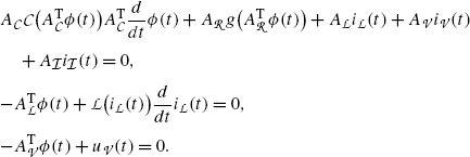 (52)
(52)The unknown variables of this system are the functions for node potentials, inductive currents, and currents of voltage sources. The remaining physical variables (such as the voltages and the resistive and capacitive currents) can be algebraically reconstructed from the solutions of the above system.
-
(b)
Modified loop analysis (MLA)
Additionally assuming that the characteristic functions g k of all resistances are strictly monotonic and surjective, the conductance function possesses some continuous and strictly monotonic inverse function
 . This function as well fulfills r(0)=0 and
Now using the component relations together with the loop-based formulation of the Kirchhoff laws, we obtain from the KVL, the component relations for resistances and inductances, and the KCL for resistive and inductive currents that

Moreover, the KCL, together with the component relation for capacitances, reads

Using these two relations together with the KVL for the voltage sources, we are led to the modified loop analysis
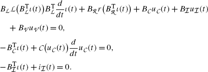 (53)
(53)The unknown variables of this system are the functions for loop currents, capacitive voltages, and voltages of current sources.


 . This function as well fulfills r(0)=0 and


2.6.2 Differential–Algebraic Equations, General Facts
Modified nodal analysis and modified loop analysis are systems of equations with a vector-valued function in one indeterminate as unknown. Some of these equations contain the derivative of certain components of the to-be-solved function, whereas other equations are of purely algebraic nature. Such systems are called differential–algebraic equations. A rigorous definition and some basics of this type are presented in the following.
Definition 6.1
(Differential–algebraic equation, solution)
Let \(U,V\subset\mathbb{R}^{n}\) be open sets, let I=[t 0,t f ) be an interval for some t f ∈(t 0,∞]. Let \(\mathcal{F}:U\times V\times I\rightarrow\mathbb{R}^{k}\) be a function. Then an equation of the form
is called a differential–algebraic equation (DAE). A function x(⋅):[t 0,ω)→V is said to be a solution of the DAE (54) if it is differentiable with \(\dot{x}(t)\) for all t∈[t 0,ω) and (54) is pointwise fulfilled for all t∈[t 0,ω).
A vector x 0∈V is called a consistent initial value if (54) has a solution with x(t 0)=x 0.
Remark 6.2
-
(i)
If \(\mathcal{F}:U\times V\times I\rightarrow\mathbb{R}^{k}\) is of the form \(\mathcal{F}(\dot{x},x,t)=\dot{x}-f(x,t)\), then (54) reduces to an ordinary differential equation (ODE). In this case, the assumption of continuity of f:V×I gives rise to the consistency of any initial value. If, moreover, f is locally Lipschitz continuous with respect to x (that is, for all (x,t)∈V×I, there exist a neighborhood \(\mathcal{U}\) and L>0 such that ∥f(x 1,τ)−f(x 2,τ)∥≤∥x 1−x 2∥ for all \((x_{1},\tau),(x_{2},\tau)\in\mathcal{U}\)), then any initial condition determines the local solution uniquely [8, §7.3]. The local Lipschitz continuity is, for instance, fulfilled if f is continuously differentiable.
-
(ii)
If \(\mathcal{F}(\cdot,\cdot,\cdot)\) is differentiable and \(\frac{d}{d\dot{x}}\mathcal{F}(\dot{x}_{0},x_{0},t_{0})\) is an invertible matrix at some \((\dot{x}_{0},x_{0},t_{0})\in U\times V\times I\), then the implicit function theorem [59, Sect. 17.8] implies that the differential–algebraic equation (54) is locally equivalent to an ODE.
Since theory of ODEs is well understood, it is—at least from a theoretical point of view—desirable to lead back a differential–algebraic equation to an ODE in a certain way. This is done in what follows.
Definition 6.3
(Derivative array, differentiation index)
Let \(U,V\subset\mathbb{R}^{n}\) be open sets, let I=[t 0,t f ) be an interval for some t f ∈(t 0,∞]. Let \(l\in\mathbb{N}\), \(\mathcal {F}:U\times V\times I\rightarrow\mathbb{R}^{k}\), and let a differential–algebraic equation (54) be given. Then the μth derivative array of ( 54 ) is given by the first μ formal derivatives of (54) with respect to time, that is,
The differential–algebraic equation (54) is said to have a differentiation index \(\mu\in\mathbb{N}\) if for all (x,t)∈V×I, there exists a unique \(\dot{x}\in V\) such that there exist \(\ddot{x},\ldots,x^{(\mu+1)}\in U\) such that \(\mathcal{F}_{\mu }(x^{(\mu+1)},x^{(\mu)},\ldots,\dot{x},x(t),t)=0\). In this case, there exists a function f:V×I→V with \((x,t)\mapsto \dot{x}\) for t, x, and \(\dot{x}\) with the above properties. The ODE
is said to be an inherent ordinary differential equation of ( 54 ).
Remark 6.4
-
(i)
By the chain rule, we have
$$\begin{aligned} 0&=\frac{d}{dt}\mathcal{F}\bigl(\dot{x}(t),x(t),t\bigr) \\ &=\frac{\partial }{\partial\dot{x}}\mathcal{F}\bigl(\dot{x}(t),x(t),t\bigr)\cdot\ddot{x}(t)+ \frac{\partial}{\partial x}\mathcal{F}\bigl(\dot{x}(t),x(t),t\bigr)\cdot\dot{x}(t)\\ &\quad + \frac{\partial}{\partial t}\mathcal{F}\bigl(\dot{x}(t),x(t),t\bigr). \end{aligned}$$A further successive application of the chain and product rules leads to a derivative array of higher order.
-
(ii)
Since the inherent ODE is obtained by differentiation of the differential–algebraic equation, any solution of (54) solves (56) as well.
-
(iii)
The inherent ODE is obtained by picking equations of the μth derivative array that are explicit for the components of \(\dot{x}\). In particular, the equations in \(\mathcal{F}_{\mu}(x^{(\mu +1)}(t),x^{(\mu)}(t),\ldots,\dot{x}(t),x(t),t)=0\) that contain higher derivatives of x can be abolished. For instance, a so-called semiexplicit differential–algebraic equation, that is, a DAE of the form
$$ 0= \begin{pmatrix}\dot{x}_1(t)-f_1(x_1(t),x_2(t),t)\\f_2(x_1(t),x_2(t),t) \end{pmatrix} $$(57)may be transformed to its inherent ODE by only differentiating the equation f 2(x 1(t),x 2(t),t)=0. This yields
$$\begin{aligned} 0&=\frac{\partial}{\partial x_1}f_2\bigl(x_1(t),x_2(t),t \bigr)\dot{x}_1(t)+ \frac{\partial}{\partial x_2}f_2 \bigl(x_1(t),x_2(t),t\bigr)\dot {x}_2(t) \\ &=\frac{\partial}{\partial x_1}f_2\bigl(x_1(t),x_2(t),t \bigr)f_1\bigl(x_1(t),x_2(t),t\bigr)+ \frac{\partial}{\partial x_2}f_2\bigl(x_1(t),x_2(t),t \bigr)\dot{x}_2(t). \end{aligned}$$(58)If \(\frac{\partial}{\partial x_{2}}f_{2}(x_{1}(t),x_{2}(t),t)\) is invertible, then the system is of differentiation index μ=1, and the inherent ODE reads
$$\begin{aligned} &\begin{pmatrix}\dot{x}_1(t)\\\dot{x}_2(t) \end{pmatrix} \\ &\quad = \begin{pmatrix}f_1(x_1(t),x_2(t),t)\\ - ( \frac{\partial}{\partial x_2}f_2(x_1(t),x_2(t),t) )^{-1} \frac{\partial}{\partial x_1}f_2(x_1(t),x_2(t),t)f_1(x_1(t),x_2(t),t) \end{pmatrix} . \end{aligned}$$(59)In this case, (x 1(⋅),x 2(⋅)) solves the differential–algebraic equation (57) if and only if it solves the inherent ODE (59) and the initial value (x 10,x 20) fulfills the algebraic constraint f 2(x 10,x 20,t 0)=0.
In case of singular \(\frac{\partial}{\partial x_{2}}f_{2}(x_{1}(t),x_{2}(t),t)\), some further differentiations are necessary to obtain the inherent ODE. A semiexplicit form may then be obtained by applying a state space transformation \(\bar {x}(t)=T(x(t),t)\) for some differentiable mapping \(T: V\times I\rightarrow\bar{V}\) with the property that \(T(\cdot,t):V\times\bar {V}\) is bijective for all t∈I and, additionally, by applying some suitable mapping \(W:\mathbb{R}^{k}\times I\times I\rightarrow\mathbb {R}^{k}\) to the differential–algebraic equation that consists of \(\dot {x}_{1}(t)-f_{1}(x_{1}(t),x_{2}(t),t)\) and the differentiated algebraic constraint. The algebraic constraint obtained in this way is referred to as a hidden algebraic constraint. This procedure is repeated until no hidden algebraic constraint is obtained anymore. In this case, the solution set of the differential–algebraic equation (57) equals the solution set of its inherent ODE with the additional property that the initial value fulfills all algebraic and hidden algebraic constraints.
The remaining part of this subsection is devoted to a differential–algebraic equation of special structure comprising both MNA and MLA, namely
with the following properties.
Assumption 6.5
(Matrices and functions in the DAE (60))
Given are matrices \(E\in\mathbb{R}^{n_{1},m_{1}}\), \(A\in\mathbb {R}^{n_{1},m_{2}}\), \(B_{2}\in \mathbb{R}^{n_{1},n_{2}}\), \(B_{3}\in\mathbb{R}^{n_{1},n_{3}}\) and continuously differentiable functions \(\alpha:\mathbb{R}^{m_{1}}\rightarrow\mathbb{R}^{m_{1},m_{1}}\), \(\beta:\mathbb{R} ^{n_{2}}\rightarrow\mathbb{R}^{n_{2},n_{2}}\), and \(\rho:\mathbb {R}^{m_{2}}\rightarrow\mathbb{R} ^{m_{2}}\) such that
-
(a)
\(\operatorname{rank}[\, E\,,\,A\,,\,B_{2}\,,\,B_{3}\,]=n_{1}\);
-
(b)
\(\operatorname{rank}B_{3}=n_{3}\);
-
(c)
α(z 1)>0, β(z 2)>0 for all \(z_{1}\in\mathbb{R}^{m_{1}}\), \(z_{2}\in\mathbb{R}^{m_{2}}\);
-
(d)
ρ′(z)+(ρ′)T(z)>0 for all \(z\in\mathbb{R}^{n_{2}}\).
Next we analyze the differentiation index of differential–algebraic equations of type (60).
Theorem 6.6
Let a differential–algebraic equation (60) be given and assume that matrices \(E\in\mathbb{R}^{n_{1},m_{1}}\), \(A\in\mathbb{R}^{n_{1},m_{2}}\), \(B_{2}\in\mathbb{R}^{n_{1},n_{2}}\), \(B_{3}\in\mathbb{R}^{n_{1},n_{3}}\) and functions \(\alpha :\mathbb{R}^{m_{1}}\rightarrow\mathbb{R}^{m_{1},m_{1}}\), \(\rho:\mathbb {R}^{m_{2}}\rightarrow\mathbb{R} ^{m_{2},m_{2}}\), \(\beta:\mathbb{R}^{n_{2}}\rightarrow\mathbb{R}^{n_{2},n_{2}}\) have the properties as in Assumptions 6.5. Then, for the differentiation index μ of (60), we have
-
(a)
μ=0 if and only if n 3=0 and \(\operatorname{rank}E=n_{1}\).
-
(b)
μ=1 if and only if it is not zero and
$$ \operatorname{rank}[ E, A, B_3]=n_1\ \textit{and}\ \ker\bigl[E^{\mathrm{T}}, B_3\bigr]=\ker E^{\mathrm{T}}\times\{0\} . $$(61) -
(c)
μ=2 if and only if μ∉{0,1}.
We need the following auxiliary results for the proof of the above statement.
Lemma 6.7
Let \(A\in\mathbb{R}^{n_{1},m}\), \(B\in\mathbb{R}^{n_{1},n_{2}}\), \(C\in \mathbb{R}^{m,m}\) with C+C T>0. Then for
we have
In particular, M is invertible if and only if kerA∩kerB T={0} and kerB={0}.
Proof
The inclusion “⊂” in (62) is trivial. To show that the converse subset relation holds as well, assume that x∈kerM and partition
according to the block structure of M. Then we obtain
whence, by
we have A T x 1=0. The equation Mx=0 then implies that Bx 2=0 and B T x 1=0. □
Note that, by setting n 2=0 in Lemma 6.7, we obtain kerACA T=kerA T.
Lemma 6.8
Let matrices \(E\in\mathbb{R}^{n_{1},m_{1}}\), \(A\in\mathbb {R}^{n_{1},m_{2}}\), \(B_{2}\in\mathbb{R} ^{n_{1},n_{2}}\), \(B_{3}\in\mathbb{R}^{n_{1},n_{3}}\) and functions \(\alpha :\mathbb{R} ^{m_{1}}\rightarrow\mathbb{R}^{m_{1},m_{1}}\), \(\rho:\mathbb {R}^{m_{2}}\rightarrow\mathbb{R}^{m_{2},m_{2}}\), \(\beta:\mathbb{R}^{n_{2}}\rightarrow\mathbb{R}^{n_{2},n_{2}}\) with the properties as in Assumptions 6.5 be given. Further, let
be matrices with full column rank and
Then we have:
-
(a)
The matrices \([W,\ \mathcal{W}]\), \([W_{1},\ \mathcal {W}_{1}]\), and \([W_{2},\mathcal{W}_{2}]\) are invertible;
-
(b)
\(\ker E^{\mathrm{T}}\mathcal{W}=\{0\}\);
-
(c)
kerW T B 3={0} if and only if ker[E T,B 3]=kerE T×{0};
-
(d)
WW 1 has full column rank, and \(\operatorname{im}WW_{1}=\ker[ E,A,B_{3}]^{\mathrm{T}}\);
-
(e)
\(\ker\mathcal{W}_{1}^{\mathrm{T}}Z^{\mathrm{T}}B_{3}\mathcal {W}_{2}=\{0\}\);
-
(f)
\(\ker[A,B_{3}\mathcal{W}_{2}]^{\mathrm{T}} W\mathcal{W}_{1}=\{ 0\}\);
-
(g)
\(\ker B_{2}^{\mathrm{T}}WW_{1}=\{0\}\);
-
(h)
\(\ker\mathcal{W}^{\mathrm{T}}B_{3}W_{2}=\{0\}\).
Proof
-
(a)
The statement for \([\,W\,,\,\mathcal{W}\,]\) follows by the fact that both W and \(\mathcal{W}\) have full column rank together with
$$\operatorname{im}W=\ker E^{\mathrm{T}}=(\operatorname{im}E)^\bot =( \operatorname{im}\mathcal{W})^\bot. $$The invertibility of the matrices \([W_{1},\ \mathcal{W}_{1}]\) and \([W_{2},\ \mathcal{W}_{2}]\) follows by the same arguments.
-
(b)
Let \(x\in\ker E^{\mathrm{T}}\mathcal{W}\). Then, by the definition of W and \(\mathcal{W}\), \(\mathcal{W}x\in\ker E^{\mathrm {T}}\) and \(\mathcal{W}x\in\operatorname{im}\mathcal {W}=\operatorname{im}E=(\ker E^{\mathrm{T}})^{\bot}\), and thus \(\mathcal{W}x=0\). Since \(\mathcal{W}\) has full column rank, we have x=0.
-
(c)
Assume that kerW T B 3={0}, and let \(x_{1}\in \mathbb{R} ^{n_{1}}\), \(x_{3}\in\mathbb{R}^{n_{3}}\) with
$$ \begin{bmatrix}E^{\mathrm{T}}&B_3 \end{bmatrix} \begin{pmatrix}x_1\\x_3 \end{pmatrix} =0. $$Multiplication of this equation from the left by W T leads to W T B 3 x 3=0, and thus x 3=0.
To prove the converse direction, assume that W T B 3 x 3=0. Then
$$B_3x_3\in\ker W^{\mathrm{T}}=(\operatorname{im}W)^\bot= \bigl(\ker E^{\mathrm{T}}\bigr)^\bot=\operatorname{im}E. $$Hence, there exists \(x_{1}\in\mathbb{R}^{m_{1}}\) such that Ex 1=B 3 x 3, that is,
$$\begin{pmatrix}-x_1\\x_3 \end{pmatrix} \in\ker \begin{bmatrix}E&B_3 \end{bmatrix} =\ker E\times\{0\}, $$whence x 3=0.
-
(d)
The matrix WW 1 has full column rank as a product of matrices with full column rank.
The inclusion \(\operatorname{im}WW_{1}\subset\ker[E,A, B_{3}]^{\mathrm{T}}\) follows from
$$\begin{bmatrix}E^{\mathrm{T}}\\ A^{\mathrm{T}}\\ B_3^{\mathrm{T}} \end{bmatrix} WW_1= \begin{bmatrix}(E^{\mathrm{T}}W)W_1\\ \bigl(\bigl[ {\scriptsize\begin{matrix}A^{\mathrm{T}}\cr B_3^{\mathrm{T}}\end{matrix}}\bigr] W \bigr)W_1 \end{bmatrix} =0. $$To prove \(\operatorname{im}WW_{1}\supset\ker[E,\ A,\ B_{3}]^{\mathrm{T}}\), assume that x∈ker[E, A, B 3]T. Since, in particular, x∈kerE T, there exists \(y\in\mathbb{R}^{p}\) with x=Wy, and thus
$$\begin{bmatrix}A^{\mathrm{T}}\\B_3^{\mathrm{T}} \end{bmatrix} Wy=0. $$By the definition of W 2, there exists \(y\in\mathbb{R}^{p_{2}}\) with y=W 2 z, and thus
$$x=WW_2z\in\operatorname{im}WW_2. $$ -
(c)
Assume that \(z\in\mathbb{R}^{p_{2}}\) with \(\mathcal {W}_{1}^{\mathrm {T}}W^{\mathrm{T}}B_{3}\mathcal{W}_{2}z=0\). Then
$$\begin{aligned} W^{\mathrm{T}}B_3\mathcal{W}_2z\in \ker\mathcal{W}_1^{\mathrm {T}}&=(\operatorname{im} \mathcal{W}_1)^\bot \\ &=\bigl(\operatorname {im}W^{\mathrm{T}}[A,\ B_3] \bigr)^\bot\\ &=\ker[A,\ B_3]^{\mathrm {T}}W\subset\ker B_3^{\mathrm{T}}W=\bigl(\operatorname{im}W^{\mathrm {T}}B_3 \bigr)^\bot, \end{aligned}$$whence
$$W^{\mathrm{T}}B_3\mathcal{W}_2z\in\bigl( \operatorname{im}W^{\mathrm {T}}B_3\bigr)^\bot\cap \operatorname{im}W^{\mathrm{T}}B_3=\{0\}. $$This implies \(W^{\mathrm{T}}B_{3}\mathcal{W}_{2}z=0\), and thus
$$\mathcal{W}_2z\in\ker W^{\mathrm{T}}B_3=\operatorname {im}W_2=(\operatorname{im}W_2)^\bot. $$Therefore, we have \(\mathcal{W}_{2}z\in\operatorname{im}W_{2}\cap \operatorname{im}\mathcal{W}_{2}=\{0\}\). The property of \(\mathcal {W}_{2}\) having full column rank then implies z=0.
-
(f)
Let \(z\in\ker(A^{\mathrm{T}}W)\cap\ker B_{3}^{\mathrm{T}}W\). Since Wz∈kerE by the definition of W, we have
$$Wz\in\ker \begin{bmatrix}E^{\mathrm{T}}\\A^{\mathrm{T}}\\B_3^{\mathrm{T}} \end{bmatrix} =\{0\}, $$whence z=0.
-
(g)
Let \(z\in\ker B_{2}^{\mathrm{T}}WW_{1}\). Then \(WW_{1}\in\ker B_{2}^{\mathrm{T}}\), and, by assertion d),
$$WW_1z\in\ker[E, A, B_2]^{\mathrm{T}}. $$By the assumption that [E, A, B 2, B 3] has full row rank we now obtain that WW 1 z=0. By the property of WW 1 having full column rank (see (d)) we may infer that z=0.
-
(h)
Assume that \(z\ker\mathcal{W}^{\mathrm{T}}B_{3}W_{2}\). Then \(W_{2}z\in\ker\mathcal{W}^{\mathrm{T}}B_{3}\), and W 2 z∈kerW T B 3 by the definition of W 2. Thus, we have
$$W_2z\in\ker[W, \mathcal{W}]^{\mathrm{T}}B_3, $$and, by the invertibility of \([W,\ \mathcal{W}]\) (see (a)), we can conclude that
$$W_2z\in\ker B_3=\{0\}. $$The property of Z 2 having full column rank then gives rise to z=0. □
Now we prove Theorem 6.6.
Proof of Theorem 6.6
-
(a)
First assume that E has full row rank and n 3=0. Then by Lemma 6.7 we see that the matrix Eα(E T x 1)E T is invertible for all \(x_{1}\in\mathbb{R}^{n_{1}}\). Since, furthermore, the last equation in (60) is trivial, the differential–algebraic equation (60) is already equivalent to the ordinary differential equation
$$ \begin{aligned}[c] \dot{x}_1(t)&=-\bigl(E \alpha \bigl(E^{\mathrm{T}}x_1(t)\bigr)E^{\mathrm {T}} \bigr)^{-1} \bigl( A\rho\bigl(A^{\mathrm{T}}x_1(t) \bigr)+B_2x_2(t)\\ &\quad +B_3x_3(t)+f_1(t) \bigr), \\ \dot{x}_2(t)&=\beta\bigl(x_2(t)\bigr)^{-1}B_2^{\mathrm{T}}x_1(t). \end{aligned} $$(64)Consequently, the differentiation index of (60) is zero in this case.
To prove the converse statement, assume that kerE T≠{0} or n 3>0. The first statement implies that no derivatives of the components of x 1(t) that are in the kernel of E T occur, whereas the latter assumption implies that (60) does not contain any derivatives of x 3 (which is now a vector with at least one component). Hence, some differentiations of the equations in (60) are needed to obtain an ordinary differential equation, and the differentiation index of (60) is consequently larger than zero.
-
(b)
Here (and in part (c)) we will make use of the (trivial) fact that, for invertible matrices W and T of suitable size, the differentiation indices of the DAEs \(\mathcal{F}(\dot {x}(t),x(t),t)=0\) and \(W\mathcal{F}(T\dot{z}(t),Tz(t),t)=0\) coincide.
Let \(W\in\mathbb{R}^{n_{1},p}\) and \(\mathcal{W}\in\mathbb {R}^{n_{1},\widetilde {p}}\) be matrices of full column rank with the properties as in (63a), (63b). Using Lemma 6.8, we see that there exists a unique decomposition
$$x_1(t)=Wx_{11}(t)+\mathcal{W}x_{12}(t). $$By a multiplication of the first equation in (60) respectively from the left by W T and \(\mathcal {W}^{\mathrm{T}}\), we can make use of the initial statement to see that the index of (60) coincides with the index of the differential–algebraic equation
$$\begin{aligned} 0&=\mathcal{W}^{\mathrm{T}}E \alpha\bigl(E^{\mathrm{T}}\mathcal {W}^{\mathrm{T}}x_{12}(t)\bigr)E^{\mathrm{T}}\mathcal{W} \dot{x}_{12}(t)+ \mathcal{W}^{\mathrm{T}}A\rho\bigl(A^{\mathrm{T}}Wx_{11}(t)+A^{\mathrm {T}} \mathcal{W}x_{12}(t)\bigr) \\ &\quad+\mathcal {W}^{\mathrm{T}}B_2x_2(t)+ \mathcal{W}^{\mathrm{T}}B_3x_3(t)+\mathcal {W}^{\mathrm{T}}f_1(t), \end{aligned}$$(65a)$$\begin{aligned} 0&=\beta\bigl(x_2(t)\bigr)\dot{x}_2(t) -B_2^{\mathrm {T}}Wx_{11}(t)-B_2^{\mathrm{T}} \mathcal{W}x_{12}(t) , \end{aligned}$$(65b)$$\begin{aligned} 0&= W^{\mathrm{T}}A\rho \bigl(A^{\mathrm{T}}Wx_{11}(t)+A^{\mathrm{T}}\mathcal {W}x_{12}(t)\bigr) \\ &\quad +W^{\mathrm {T}}B_2x_2(t)+W^{\mathrm{T}}B_3x_3(t)+W^{\mathrm{T}}f_1(t) , \end{aligned}$$(65c)$$\begin{aligned} 0&=-B_3^{\mathrm {T}}Wx_{11}(t)+B_3^{\mathrm{T}} \mathcal{W}x_{12}(t)+f_3(t). \end{aligned}$$(65d)Now we show that, under the assumptions that the index of the differential–algebraic equation (65a)–(65d) is nonzero and the rank conditions in (61) hold, the index of the DAE (65a)–(65d) equals one:
Using Lemma 6.7, we see that Eqs. (65a) and (65b) can be solved for \(\dot{x}_{12}(t)\) and \(\dot{x}_{2}(t)\), that is,
$$\begin{aligned} \dot{x}_{12}(t)&=-\bigl(\mathcal{W}^{\mathrm{T}}E \alpha \bigl(E^{\mathrm {T}}\mathcal{W}^{\mathrm{T}}x_{12}(t) \bigr)E^{\mathrm{T}}\mathcal {W}\bigr)^{-1}\mathcal{W}^{\mathrm{T}} \bigl( A\rho\bigl(A^{\mathrm{T}}Wx_{11}(t) \\ &\quad +A^{\mathrm{T}}\mathcal {W}x_{12}(t)\bigr) +B_2x_2(t)+B_3x_3(t)+f_1(t) \bigr), \end{aligned}$$(66a)$$\begin{aligned} \dot{x}_2(t)&=\beta\bigl(x_2(t)\bigr)^{-1}B_2^{\mathrm{T}} \bigl(Wx_{11}(t)+\mathcal{W}x_{12}(t) \bigr). \end{aligned}$$(66b)For convenience and better overview, we will further use the following abbreviations:
$$\begin{aligned} & \rho\bigl(A^{\mathrm{T}}Wx_{11}(t)+A^{\mathrm{T}} \mathcal {W}x_{12}(t)\bigr)\rightsquigarrow\rho, \\ &\rho'\bigl(A^{\mathrm{T}}Wx_{11}(t)+A^{\mathrm{T}} \mathcal {W}x_{12}(t)\bigr)\rightsquigarrow\rho', \\ &\alpha\bigl(E^{\mathrm{T}}\mathcal{W}^{\mathrm {T}}x_{12}(t) \bigr)\rightsquigarrow\alpha, \\ &\beta\bigl(x_2(t)\bigr)\rightsquigarrow\beta. \end{aligned}$$The first-order derivative array \(\mathcal{F}_{1}(x^{(2)}(t),\dot {x}(t),x(t),t)\) of the DAE (60) further contains the time derivatives of (65c) and (65d), which can, in compact form and by making further use of (66a), (66b), be written as
$$\begin{aligned} &\underbrace{ \begin{bmatrix}W^{\mathrm{T}}A\rho'A^{\mathrm{T}}W&W^{\mathrm {T}}B_3\\-B_3^{\mathrm{T}}W&0 \end{bmatrix} }_{=:M} \begin{pmatrix}\dot{x}_{11}(t)\\ \dot{x}_3(t) \end{pmatrix} \\ &\quad =- \begin{pmatrix}W^{\mathrm{T}}A\rho'A^{\mathrm{T}}\mathcal{W}\dot {x}_{12}(t)+W^{\mathrm{T}}B_2\dot{x}_2(t)+W^{\mathrm{T}}\dot {f}_2(t)\\ B_3^{\mathrm{T}}\mathcal{W}\dot{x}_{12}(t)+\dot{f}_3(t) \end{pmatrix} \\ &\quad = \begin{pmatrix}W^{\mathrm{T}}A\rho'A^{\mathrm{T}}\mathcal {W}(\mathcal{W}^{\mathrm{T}}E \alpha E^{\mathrm{T}}\mathcal {W})^{-1}\mathcal{W}^{\mathrm{T}} ( A\rho+B_2x_2(t)+B_3x_3(t)+f_1(t) ),\\ B_3^{\mathrm{T}}\mathcal {W}(\mathcal{W}^{\mathrm{T}}E \alpha E^{\mathrm{T}}\mathcal {W})^{-1}\mathcal{W}^{\mathrm{T}} ( A\rho+B_2x_2(t)+B_3x_3(t)+f_1(t) )+\dot{f}_3(t) \end{pmatrix} \\ &\qquad {}- \begin{pmatrix}W^{\mathrm{T}}B_2\beta^{-1}B_2^{\mathrm{T}} (Wx_{11}(t)+\mathcal{W}x_{12}(t) )+\mathcal{W}^{\mathrm {T}}\dot{f}_2(t)\\ 0 \end{pmatrix} . \end{aligned}$$(67)Since, by assumption, there holds (61), we obtain from Lemma 6.8 (c) and (d) that
$$\ker W^{\mathrm{T}}B_3=\{0\}\quad \text{and}\quad \ker[A, B_3 ]^{\mathrm{T}}W=\{0\}. $$Then by using of ρ′+ρ′T>0 we may infer from Lemma 6.7 that M is invertible. As a consequence, \(\dot {x}_{11}(t)\) and \(\dot{x}_{3}(t)\) can be expressed by suitable functions depending on x 12(t), x 2(t), and t. This implies that the index of the differential–algebraic equation equals one.
Now we show that conditions (61) are also necessary for the index of the differential–algebraic equation (60) not to exceed one:
Consider the first-order derivative array \(\mathcal {F}_{1}(x^{(2)}(t),\dot{x}(t),x(t),t)\) of the DAE (60). Aiming to construct an ordinary differential equation (56) for
$$x(t)= \begin{pmatrix}x_1(t)\\x_2(t)\\x_3(t) \end{pmatrix} $$from \(\mathcal{F}_{1}(x^{(2)}(t),\dot{x}(t),x(t),t)\), it can be seen that the derivatives of Eqs. (66a) and (66b) cannot be used to form the inherent ODE (the derivatives of these equations explicitly contain the second derivatives of x 12(t) and x 2(t)). As a consequence, the inherent ODE is formed by Eqs. (66a), (66b) and (67). Aiming to seek for a contradiction, assume that one of the conditions in (61) is violated:
In case of \(\operatorname{rank}[ E, A, B_{3}]< n_{1}\), Lemma 6.8 (d) implies that
$$\ker[E, B_3]^{\mathrm{T}}W\neq\{0\}. $$Now consider matrices W 1, \(\mathcal{W}_{1}\) of full column rank with the properties as in (63a), (63b). By Lemma 6.8 (a) there exists a unique decomposition
$$x_{11}(t)=W_1x_{111}(t)+\mathcal{W}_1x_{112}(t). $$Then the right-hand side of Eq. (67) reads
$$ \begin{bmatrix}W^{\mathrm{T}}A\rho'A^{\mathrm{T}}W\mathcal {W}_1&0&W^{\mathrm{T}}B_3\\-B_3^{\mathrm{T}}WW_1&0&0 \end{bmatrix} \begin{pmatrix}\dot{x}_{111}(t)\\\dot{x}_{112}(t)\\ \dot{x}_3(t) \end{pmatrix} . $$Consequently, it is not possible to use the first-order derivative array to express \(\dot{x}_{112}(t)\) as a function of x(t). This is a contradiction to the index of the differential–algebraic equation (60) being at most one.
In case of ker[E T,B 3]≠kerE T×{0}, by Lemma 6.8 (c) we have ker(W T B 3)≠{0}. Consider matrices W 2, \(\mathcal {W}_{2}\) of full column rank with the properties as in (63a), (63b). By Lemma 6.8 a) there exists a unique decomposition
$$x_{3}(t)=W_2x_{31}(t)+\mathcal{W}_2x_{32}(t). $$Then the right-hand side of Eq. (67) reads
$$ \begin{bmatrix}W^{\mathrm{T}}A\rho'A^{\mathrm{T}}W&W^{\mathrm {T}}B_3\mathcal{W}_2&0\\-B_3^{\mathrm{T}}W&0&0 \end{bmatrix} \begin{pmatrix}\dot{x}_{11}(t)\\ \dot{x}_{31}(t)\\ \dot{x}_{32}(t) \end{pmatrix} . $$Consequently, it is not possible to use the first-order derivative array to express \(\dot{x}_{32}(t)\) as a function of x(t). This is a contradiction to the index of the differential–algebraic equation (60) being at most one.
-
(c)
To complete the proof, we have to show that the inherent ODE can be constructed from the second-order derivative array \(\mathcal {F}_{2}(x^{(3)}(t),x^{(2)}(t),\dot{x}(t),x(t),t)\) of the DAE (60). With the matrices W, \(\mathcal{W}\), W 1, \(\mathcal{W}_{1}\), W 2, \(\mathcal{W}_{2}\) and the corresponding decompositions, a multiplication of (67) from the left with
$$ \begin{bmatrix}\mathcal{W}_1^{\mathrm{T}}&0\\0&\mathcal {W}_2^{\mathrm{T}} \end{bmatrix} $$leads to
$$\begin{aligned} &\underbrace{ \begin{bmatrix}\mathcal{W}_1^{\mathrm{T}}W^{\mathrm{T}}A\rho 'A^{\mathrm{T}}W\mathcal{W}_1&\mathcal{W}_1^{\mathrm{T}}W^{\mathrm {T}}B_3\mathcal{W}_2\\-\mathcal{W}_2^{\mathrm{T}}B_3^{\mathrm {T}}W\mathcal{W}_1&0 \end{bmatrix} }_{=:M_1} \begin{pmatrix}\dot{x}_{112}(t)\\ \dot{x}_{32}(t) \end{pmatrix} \\ &\quad = \begin{pmatrix}\mathcal{W}_1^{\mathrm{T}}W^{\mathrm{T}}A\rho 'A^{\mathrm{T}}\mathcal{W}(\mathcal{W}^{\mathrm{T}}E \alpha E^{\mathrm{T}}\mathcal{W})^{-1}\mathcal{W}^{\mathrm{T}} ( A\rho+B_2x_2(t)+B_3x_3(t)+f_1(t) )\\ \mathcal{W}_2^{\mathrm {T}}B_3^{\mathrm{T}}\mathcal{W}(\mathcal{W}^{\mathrm{T}}E \alpha E^{\mathrm{T}}\mathcal{W})^{-1}\mathcal{W}^{\mathrm{T}} ( A\rho+B_2x_2(t)+B_3x_3(t)+f_1(t) )+\mathcal{W}_2^{\mathrm {T}}\dot{f}_3(t) \end{pmatrix} \\ &\qquad {}- \begin{pmatrix}\mathcal{W}_1^{\mathrm{T}}\mathcal{W}^{\mathrm {T}}B_2\beta^{-1}B_2^{\mathrm{T}} (Wx_{11}(t)+\mathcal {W}x_{12}(t) )+\mathcal{W}_1^{\mathrm{T}}\mathcal{W}^{\mathrm {T}}\dot{f}_2(t)\\ 0 \end{pmatrix} . \end{aligned}$$(68)By Lemma 6.8 (e) and (f) we have
$$\ker\mathcal{W}_1^{\mathrm{T}}W^{\mathrm{T}}B_3 \mathcal{W}_2=\{0\} \quad \text{and}\quad \ker[A, B_3 \mathcal{W}_2]^{\mathrm{T}}=\{0\}. $$Lemma 6.7 then implies that M 1 is invertible, and, consequently, the vectors \(\dot{x}_{112}(t)\) and \(\dot{x}_{32}(t)\) are expressible by suitable functions of x 111(t), x 112(t), x 2(t), x 31(t), x 32(t), and t. It remains to show that the second-order derivative array might also be used to express \(\dot {x}_{111}(t)\) and \(\dot{x}_{31}(t)\) as functions of x 111(t), x 112(t), x 2(t), x 31(t), x 32(t), and t: A multiplication of (67) from the left by
$$ \begin{bmatrix}W_1^{\mathrm{T}}&0\\0&W_2^{\mathrm{T}} \end{bmatrix} $$yields, by making use of \(W_{1}^{\mathrm{T}}W^{\mathrm{T}}A=0\), that
$$\begin{aligned} 0&=W_1^{\mathrm{T}}W^{\mathrm{T}}B_2 \beta^{-1}B_2^{\mathrm{T}} \bigl(WW_1x_{111}(t)+W \mathcal{W}_1x_{112}(t)+\mathcal{W}x_{12}(t) \bigr) \\ &\quad +W_1^{\mathrm{T}}W^{\mathrm{T}}\dot{f}_2(t), \end{aligned}$$(69a)$$\begin{aligned} 0&=W_2^{\mathrm{T}}B_3^{\mathrm{T}}\mathcal{W} \bigl(\mathcal {W}^{\mathrm{T}}E \alpha E^{\mathrm{T}}\mathcal{W} \bigr)^{-1}\mathcal {W}^{\mathrm{T}} \\ &\quad{}\cdot \bigl( A\rho+B_2x_2(t)+B_3W_2x_{31}(t)+B_3 \mathcal {W}_2x_{32}(t)+f_1(t) \bigr)+W_2^{\mathrm{T}}\dot{f}_3(t). \end{aligned}$$(69b)The second-order derivative array of (60) contains the derivative of these equations. Differentiating (69a) with respect to time, we obtain
$$\begin{aligned} &W_1^{\mathrm{T}}W^{\mathrm{T}}B_2 \beta^{-1}B_2^{\mathrm {T}}W_1W \dot{x}_{111}(t) \\ &\quad =-W_1^{\mathrm{T}}W^{\mathrm{T}}B_2 \beta^{-1}B_2^{\mathrm{T}} \bigl(W\mathcal{W}_1 \dot{x}_{112}(t)+\mathcal{W}\dot{x}_{12}(t) \bigr) \\ &\qquad -W_1^{\mathrm{T}}W^{\mathrm{T}}B_2 \frac{d}{dt}\bigl(\beta^{-1}\bigr)B_2^{\mathrm{T}} \bigl(W\mathcal {W}_1{x}_{112}(t)+\mathcal{W} {x}_{12}(t) \bigr)-W_1^{\mathrm {T}} \mathcal{W}^{\mathrm{T}}\ddot{f}_2(t). \end{aligned}$$(70)Using Lemma 6.8 (g) and Lemma 6.7, we see that the matrix
$$W_1^{\mathrm{T}}W^{\mathrm{T}}B_2 \beta^{-1}B_2^{\mathrm{T}}WW_1\in \mathbb{R}^{p_1,p_1} $$is invertible. By using the quotient and chain rule it can be inferred that \(\frac{d}{dt}(\beta^{-1})\) is expressible by a suitable function depending on x 2(t) and \(\dot{x}_{2}(t)\). Consequently, the derivative of x 111(t) can be expressed as a function depending on x 112(t), x 12(t), x 2(t), their derivatives, and t. Since, on the other hand, \(\dot{x}_{112}(t)\), \(\dot{x}_{12}(t)\), and \(\dot{x}_{2}(t)\) already have representations as functions depending on x 111(t), x 112(t), x 12(t), x 2(t), x 31(t), x 32(t), and t, this is true for \(\dot{x}_{112}(t)\) as well.
Differentiating (69b) with respect to t, we obtain
$$\begin{aligned} &W_2^{\mathrm{T}}B_3^{\mathrm{T}}\mathcal{W}\bigl( \mathcal{W}^{\mathrm {T}}E \alpha E^{\mathrm{T}}\mathcal{W} \bigr)^{-1}\mathcal{W}^{\mathrm {T}}B_3W_2 \dot{x}_{31} \\ &\quad =W_2^{\mathrm{T}}B_3^{\mathrm{T}}\mathcal{W} \bigl(\mathcal {W}^{\mathrm{T}}E \alpha E^{\mathrm{T}}\mathcal{W} \bigr)^{-1}\mathcal {W}^{\mathrm{T}} \\ &\qquad {} \cdot \bigl( A\rho'AWW_1\dot{x}_{111}(t)+A \rho'AW\mathcal{W}_1\dot {x}_{112}(t)+A \rho'A\mathcal{W}\dot{x}_{12}(t) \\ &\qquad{}+B_2\dot{x}_2(t)+B_3W_2 \dot{x}_{31}(t)+\dot{f}_1(t) \bigr) \\ &\qquad {}+W_2^{\mathrm{T}}B_3^{\mathrm{T}}\mathcal{W} { \frac {d}{dt}}\bigl(\mathcal{W}^{\mathrm{T}}E \alpha E^{\mathrm{T}} \mathcal {W}\bigr)^{-1}\mathcal{W}^{\mathrm{T}} \\ & \qquad {}\cdot \bigl( A\rho+B_2x_2(t)+B_3W_2x_{31}(t)+B_3 \mathcal {W}_2x_{32}(t)+f_1(t) \bigr)+W_2^{\mathrm{T}}\dot{f}_3(t). \end{aligned}$$Lemma 6.8 h) and Lemma 6.7 give rise to the invertibility of the matrix
$$W_2^{\mathrm{T}}B_3^{\mathrm{T}}\mathcal{W}\bigl( \mathcal{W}^{\mathrm {T}}E \alpha E^{\mathrm{T}}\mathcal{W} \bigr)^{-1}\mathcal{W}^{\mathrm {T}}B_3W_2\in \mathbb{R}^{p_2,p_2}. $$Then arguing as for the derivative of Eq. (69a), we can see that \(\dot{x}_{31}\) is expressible by a suitable function depending on x 111(t), x 112(t), x 12(t), x 2(t), x 31(t), x 32(t), and t.
This completes the proof. □
Remark 6.9
(Differentiation index of differential–algebraic equations)
-
(i)
The algebraic constraints of (60) are formed by (69a), (69b). Note that (69a) is trivial (i.e., it is an empty set of equations) if \(\operatorname{rank}E=n_{1}\). Accordingly, the hidden constraint (69a) is trivial in the case where n 3=0.
-
(ii)
The hidden algebraic constraints of (60) are formed by (69a), (69b). Note that (69a) is trivial if \(\operatorname{rank}[ E,\ A,\ B_{3}]=n_{1}\), whereas, in the case where ker[E T, B 3]=kerE T×{0}, the hidden constraint (69a) becomes trivial.
-
(iii)
From the computations in the proof of Theorem 6.6 we see that derivatives of the “right-hand side” f 1(⋅), f 3(⋅) enter the solution of the differential–algebraic equation. The order of these derivatives equals μ−1.
We close the analysis of differential–algebraic equations of type (60) by formulating the following result on consistency of initial values.
Theorem 6.10
Let a differential–algebraic equation (60) be given and assume that the matrices \(E\in\mathbb{R}^{n_{1},m_{1}}\), \(A\in\mathbb {R}^{n_{1},m_{2}}\), \(B_{2}\in\mathbb{R}^{n_{1},n_{2}}\), \(B_{3}\in\mathbb{R}^{n_{1},n_{3}}\) and functions \(\alpha :\mathbb{R}^{m_{1}}\rightarrow\mathbb{R}^{m_{1},m_{1}}\), \(\rho:\mathbb {R}^{m_{2}}\rightarrow\mathbb{R} ^{m_{2},m_{2}}\), \(\beta:\mathbb{R}^{n_{2}}\rightarrow\mathbb{R}^{n_{2},n_{2}}\) have the properties as in Assumptions 6.5. Let W, \(\mathcal{W}\), W 1, \(\mathcal{W}_{1}\), W 2, and \(\mathcal {W}_{2}\) be matrices of full column rank with the properties as in (63a), (63b). Let a continuous function \(f_{1}:[t_{0},\infty)\rightarrow\mathbb {R}^{n_{1}}\) be such that
is continuously differentiable and
is twice continuously differentiable. Further, assume that \(f_{3}:[t_{0},\infty)\rightarrow\mathbb{R}^{n_{3}}\) is continuously differentiable and such that
is twice continuously differentiable. Then the initial value
is consistent if and only if
Proof
First, assume that a solution of (60) evolves in the time interval [t 0,ω). The necessity of the consistency conditions (72a)–(72d) follows by the fact that, by (65c), (65c), (69a), (69a) and the definitions of x 111(t), x 112(t), x 12(t), x 31(t), and x 32(t), the relations
hold for all t∈[t 0,ω). The special case t=t 0 gives rise to (72a)–(72d).
To show that (72a)–(72d) is sufficient for consistency of the initialization, we prove that the inherent ODE of (72a)–(72d), together with the initial value (71) fulfilling (72a)–(72d), possesses a solution that is also a solution of the differential–algebraic equation (60):
By the construction of the inherent ODE in the proof of Theorem 6.6 we see that the right-hand side is continuously differentiable. The existence of a unique solution
is therefore guaranteed by standard results on the existence and uniqueness of solutions of ordinary differential equations.
The inherent ODE further contains the derivative of the equations in (70) with respect to time. In other words,
for all t∈[t 0,ω). Then we can infer from (72c) and (72d) together with (71) that
for all t∈[t 0,ω). Since, furthermore, Eq. (68) is a part of the inherent ODE, we can conclude that the solution pointwise fulfills Eq. (67). However, the latter equation is by construction equivalent to
Analogously to the above arguments, we can infer from (72a) and (72b) together with (71) that
for all t∈[t 0,ω). Since these equations, together with
form the differential–algebraic equation (60), the desired result is proven. □
Remark 6.11
(Relaxing Assumptions 6.5)
The solution theory for differential–algebraic equations of type (60) can be extended to the case where conditions (a) and (b) in Assumptions 6.5 are not necessarily fulfilled: Consider matrices
of full column rank such that
Then, multiplying the first equation in (60) from the left by \(\mathcal{V}_{1}\) and the third equation in (60) from the left by \(\mathcal{V}_{3}\), and setting
we obtain
Note that, by techniques similar as in the proof of Lemma 6.8, it can be shown that (73) is a differential–algebraic equation that fulfills the presumptions of Theorem 6.6 and Theorem 6.10.
On the other hand, multiplying the first equation from the left by V 1 and the third equation from the left by V 3, on the right-hand side, we obtain the constraints
or, equivalently,
Solvability of (60) therefore becomes dependent on the property of f 1(⋅) and f 3(⋅) evolving in certain subspaces. Note that the components \(\bar{x}_{1}(t)\) and \(\bar{x}_{3}(t)\) do not occur in any of the above equations. In case of existence of solutions, this part can be chosen arbitrarily. Consequently, a violation of (a) or (b) in Assumptions 6.5 causes the nonuniqueness of solutions.
2.6.3 Circuit Equations—Structural Considerations
Here we will apply our findings on differential–algebraic equations of type (60) to MNA and MLA equations. It will turn out that the index structural property of the circuit can be characterized by means of the circuit topology. The concrete behavior of the capacitance, inductance, and conductance functions does not influence the differentiation index.
In the following, we will use expressions like an “ -loop” for a loop in the circuit graph whose branch set consists only of branches corresponding to voltage sources and/or inductances. Likewise, by a
  -cutset, we mean a cutset in the circuit graph whose branch set consists only of branches corresponding to current sources and/or capacitances.
The general assumptions on the electric circuits are formulated as follows.
Assumption 6.12
(Electrical circuits)
Given is an electrical circuit with  voltage sources, \(n_{\mathcal {I}}\) current sources,
  capacitances,
  inductances,
  resistances, n nodes, and the following properties:
-
(a)
there are no \(\mathcal {I}\)-cutsets;
-
(b)
there are no
 -loops;
 -
(c)
the charge functions
 are continuously differentiable with
  for all \(u\in\mathbb{R}\);
 -
(d)
the flux functions
 are continuously differentiable with
  for all \(i\in\mathbb{R}\);
 -
(e)
the conductance functions
 are continuously differentiable with
  for all \(u\in\mathbb{R}\);
 -loops;
 are continuously differentiable with
  for all
  are continuously differentiable with
  for all
  are continuously differentiable with
  for all
 Remark 6.13
(The assumptions on circuits)
The absence of  -loops means, in a nonmathematical manner of speaking, that there are no short circuits. Indeed, a
  -loop would cause that certain voltages of the sources cannot be chosen freely (see below).
Likewise, an \(\mathcal {I}\)-cutset consequences induces further algebraic constraints on the currents of the current sources.
Note that by Lemma 4.10 (b) the absence of  -loops is equivalent to

whereas by Lemma 4.10 (a) the absence of \(\mathcal {I}\)-cutsets is equivalent to

Consequently, the MNA equations are differential–algebraic equations of type (60) with the properties described in Assumptions 6.5.
Further, we can use Lemma 4.10 (b) to see that the circuit does not contain any  -loops if and only if

A further use of Lemma 4.10 (a) implies that the absence of \(\mathcal {I}\)-cutsets is equivalent to
If, moreover, we assume that the functions  possess global inverses, which are, respectively, denoted by
  , then the MLA equations are as well differential–algebraic equations of type (60) with the properties as described in Assumptions 6.5.
Theorem 6.14
(Index of MNA equations)
Let an electrical circuit with the properties as in Assumptions 6.12 be given. Then the differentiation index μ of the MNA equations (52) exists. In particular, we have:
-
(a)
The following statements are equivalent:
-
(i)
μ=0;
-
(ii)
 and
and
 ;
; -
(iii)
the circuit neither contains
 -cutsets nor voltage sources.
-
(i)
-
(b)
The following statements are equivalent:
-
(i)
μ=1;
-
(ii)
 and
and
 ;
; -
(iii)
the circuit neither contains
 -cutsets nor
 -loops except for
 -loops.
-
(i)
-
(c)
The following statements are equivalent:
-
(i)
μ=2;
-
(ii)
 or
or
 ;
; -
(iii)
the circuit contains
 -cutsets or
 -loops which are no pure
 -loops.
-
(i)
 and
and
 ;
; -cutsets nor voltage sources.
 and
and
 ;
; -cutsets nor
 -loops except for
 -loops.
 or
or
 ;
; -cutsets or
 -loops which are no pure
 -loops.
Proof
Since the MNA equations (52) form a differential–algebraic equation of type (60) with the properties as in Assumptions 6.5, the equivalences between (i) and (ii) in (a), (b), and (c) are immediate consequences of Theorem 6.6.
The equivalence of (a) (ii) and (a) (iii) follows from the definition of  and the fact that, by Lemma 4.10 (a), the absence of
  -cutsets (which is the same as the absence of
  -cutsets since the circuit does not contain any voltage sources) is equivalent to
  .
.
Since, by Lemma 4.10 (a),

and, by Lemma 4.11,

assertions (b) (ii) and (b) (iii) are equivalent. By the same arguments we see that (c) (ii) and (c) (iii) are equivalent as well. □
Theorem 6.15
(Index of MLA equations)
Let an electrical circuit with the properties as in Assumptions 6.12 be given. Moreover, assume that the functions

possess global inverses, which are, respectively, denoted by

Then the differentiation index μ of the MLA equations (53) exists. In particular, we have:
-
(a)
The following statements are equivalent:
-
(i)
μ=0;
-
(ii)
 and
\(n_{\mathcal {I}}=0\);
and
\(n_{\mathcal {I}}=0\); -
(iii)
the circuit contains neither
 -loops nor current sources.
-
(i)
-
(b)
The following statements are equivalent:
-
(i)
μ=1;
-
(ii)
 and
and
 ;
; -
(iv)
the circuit contains neither
 -loops nor
 -cutsets except for
 -cutsets.
-
(i)
-
(c)
The following statements are equivalent:
-
(i)
μ=2;
-
(ii)
 or
or
 ;
; -
(iii)
the circuit contains
 -loops or
 -cutsets that are not pure
 -loops.
-
(i)
 and
and
 -loops nor current sources.
 and
and
 ;
; -loops nor
 -cutsets except for
 -cutsets.
 or
or
 ;
; -loops or
 -cutsets that are not pure
 -loops.
Proof
The MLA equations (52) form a differential–algebraic equation of type (60) with the properties as formulated in Assumptions 6.5. Hence, the equivalences of (i) and (ii) in (a), (b), and (c) are immediate consequences of Theorem 6.6.
The equivalence of (a) (ii) and (a) (iii) follows from the definition of \(n_{\mathcal {I}}\) and the fact that, by Lemma 4.10 (b), the absence of  -loops (which is the same as the absence of
  -cutsets since the circuit does not contain any current sources), is equivalent to
  .
.
By Lemma 4.12 we have

and by Lemma 4.11 we have

As a consequence, assertions (b) (ii) and (b) (iii) are equivalent. By the same arguments, we see that (c) (ii) and (c) (iii) are equivalent as well. □
Next, we aim to apply Theorem 6.10 to explicitly characterize consistency of the initial values of the MNA and MLA equations. For the result about consistent initialization of the MNA equations, we introduce the matrices of full column rank

such that

The following result (as the corresponding result on MLA equations) is an immediate consequence of Theorem 6.10.
Theorem 6.16
Let an electrical circuit with the properties as in Assumptions
6.12
be given. Let
 ,
,  ,
,  ,
,  ,
,  , and
, and
 be matrices of full column rank with the properties as in (80a), (80b). Let
\(i_{\mathcal {I}} [t_{0},\infty)\rightarrow\mathbb{R}^{n_{\mathcal {I}}}\)
be continuous and such that
be matrices of full column rank with the properties as in (80a), (80b). Let
\(i_{\mathcal {I}} [t_{0},\infty)\rightarrow\mathbb{R}^{n_{\mathcal {I}}}\)
be continuous and such that

is continuously differentiable and

is twice continuously differentiable.
Further, assume that
 is continuously differentiable and such that

is twice continuously differentiable.
Then the initial value

is consistent if and only if


To formulate a corresponding result for the MLA, consider the matrices of full column rank

such that

These matrices will be used to characterize consistency of the initial values of the MLA system.
Theorem 6.17
Let an electrical circuit with the properties as in Assumptions
6.12
be given. Moreover, assume that the functions
 possess global inverses, which are, respectively, denoted by
 . Let
. Let
 ,
,  ,
,  ,
,  ,
,  , and
, and
 be matrices of full column rank with the properties as in (80a), (80b). Let
\(i_{\mathcal {I}}:[t_{0},\infty)\rightarrow\mathbb{R}^{n_{\mathcal {I}}}\)
be continuously differentiable and such that
be matrices of full column rank with the properties as in (80a), (80b). Let
\(i_{\mathcal {I}}:[t_{0},\infty)\rightarrow\mathbb{R}^{n_{\mathcal {I}}}\)
be continuously differentiable and such that

is twice continuously differentiable.
Further, assume that
 is continuous and such that

is continuously differentiable and

is twice continuously differentiable.
Then the initial value

is consistent if and only if


Remark 6.18
( -loops and \(\mathcal {I}\)-cutsets)
If a circuit contains  -loops and \(\mathcal {I}\)-cutsets (compare Remark 6.13), we may apply the findings in Remark 6.11 to extract a differential–algebraic equation of type (60) that satisfies Assumptions 6.5. More precisely, we consider matrices of full column rank

such that

Then, by making the ansatz

we see that the functions \(\bar{\phi}(\cdot)\) and  can be chosen arbitrarily, whereas the solvability of the MNA equations (52) is equivalent to

The other components then satisfy

To perform analogous manipulations to the MLA equations, consider matrices full column rank

such that

Then, by making the ansatz

we see that the functions \(\bar{\iota}(\cdot)\) and \(\bar{i}_{\mathcal {I}}(\cdot)\) can be chosen arbitrarily, whereas the solvability of the MLA equations (53) is equivalent to

The other components then satisfy

Note that both ansatzes have the practical interpretation that for each  -loop, one voltage is constrained (for instance, by the equation
  or equivalently by
  ), and one current can be chosen arbitrarily.
An according interpretation can be made for \(\mathcal {I}\)-cutsets: In each \(\mathcal {I}\)-cutset, one current is constrained (for instance, by the equation  or equivalently by \(\overline{Y}_{\mathcal {I}}i_{\mathcal {I}}(\cdot)\equiv0\)), and one voltage can be chosen arbitrarily.
To illustrate this by means of an example, the configuration in Fig. 15 causes \(i_{\mathcal {I}1}(\cdot)=i_{\mathcal {I}2}(\cdot)\), whereas the reduced MLA equations (87) contain \(u_{\mathcal {I}1}(\cdot)+u_{\mathcal {I}2}(\cdot)\) as a component of \(\widetilde{u}_{\mathcal {I}}(\cdot)\). Likewise, the configuration in Fig. 16 causes  , whereas the reduced MNA equations (86) contain
  as a component of
  .
.

Serial interconnection of current sources

Parallel interconnection of voltage sources
Remark 6.19
(Index one conditions in MNA and MLA)
-
(i)
The property that
 -loops and
  -loops cause higher index is quite intuitive from a physical perspective: In a
  -loop, the capacitive currents are prescribed by the derivatives of the voltages of the voltage sources (see Fig. 17). In an
  -cutset, the inductive voltages are prescribed by the derivatives of the currents of the current sources (see Fig. 18).
 Fig. 17 
Parallel interconnection of a voltage source and a capacitance
Fig. 18 
Serial interconnection of a current source and an inductance
-
(ii)
An interesting feature is that
 -cutsets (including pure
  -cutsets, see Fig. 19) cause that the MNA system has differentiation index two, whereas the corresponding index two condition for the MLA system is the existence of
  -cutsets without pure
  -cutsets.
 Fig. 19 
 -cutset
For
 -loops, situation becomes, roughly speaking, vice versa:
  -loops (including pure
  -loops, see Fig. 20) cause that the MLA system has differentiation index two, whereas the corresponding index two condition for the MNA system is the existence of
  -loops without pure
  -loops.
 Fig. 20 
 -loop
-loop
 -loops and
  -loops cause higher index is quite intuitive from a physical perspective: In a
  -loop, the capacitive currents are prescribed by the derivatives of the voltages of the voltage sources (see Fig.
  -cutset, the inductive voltages are prescribed by the derivatives of the currents of the current sources (see Fig.

 -cutsets (including pure
  -cutsets, see Fig.
  -cutsets without pure
  -cutsets.
 -cutset
 -loops, situation becomes, roughly speaking, vice versa:
  -loops (including pure
  -loops, see Fig.
  -loops without pure
  -loops.
 -loop
-loopRemark 6.20
(Consistency conditions for MNA and MLA equations)
Note that, for an electrical circuit that contains neither  -loops nor
  -cutsets, the following holds for the consistency conditions (82a)–(82d) and (85a)–(85d):
-
(i)
Equation (82a) becomes trivial (that is, it contains no equations) if and only if the circuit does not contain any
 -cutsets.
 -
(ii)
Equation (82b) becomes trivial if and only if the circuit does not contain any voltage sources.
-
(iii)
Equation (82c) becomes trivial if and only if the circuit does not contain any
 -cutsets.
 -
(iv)
Equation (82d) becomes trivial if and only if the circuit does not contain any
 -loops except for pure
  -loops.
 -
(v)
Equation (85a) becomes trivial if and only if the circuit does not contain any
 -loops.
 -
(vi)
Equation (85b) becomes trivial if and only if the circuit does not contain any current sources.
-
(vii)
Equation (85c) becomes trivial if and only if the circuit does not contain any
 -loops.
 -
(viii)
Equation (85d) becomes trivial if and only if the circuit does not contain any
 -cutsets except for pure
  -cutsets.
 -cutsets.
 -cutsets.
 -loops except for pure
  -loops.
 -loops.
 -loops.
 -cutsets except for pure
  -cutsets.
We finally glance at the energy exchange of electrical circuits: Consider again the MNA equations

A multiplication of the first equation from the left by ϕ
T(t), of the second equation from the left by  , and of the third equation from the left by \(i_{\mathcal {I}}^{\mathrm {T}}(t)\) and then a summation and according integration of these equations yields

Due to  ,
,  , this equation simplifies to

Using the nonnegativity of  (see (47)) and, furthermore, the representations (40), (44), and (48a) for capacitive and inductive energy, we obtain

where  and
and  are the storage functions for capacitive and, respectively, inductive energy. Since, the integral of the product between voltage and current represents the energy consumptions of a specific element, relation (89) represents an energy balance of a circuit: The energy gain at capacitances and inductances is less than or equal to the energy provided by the voltage and current sources. Note that the above deviations can alternatively done on the basis of the modified loop analysis.
The difference between consumed and stored energy is given by

which is nothing but the energy lost at the resistances. Note that, for circuits without resistances (the so-called LC resonators), the balance (89) becomes an equation. In particular, the sum of capacitive and inductive energies remains constant if the sources are turned off.
Remark 6.21
(Analogies between Maxwell’s and circuit equations)
The energy balance (89) can be regarded as a lumped version of the corresponding property of Maxwell’s equations; see (5a), (5b). Note that this is not the only parallelism between circuits and electromagnetic fields: For instance, Tellegen’s law has a field version and a circuit version; see (12) and (28).
It seems to be an interesting task to work out these and further analogies between electromagnetic fields and electric circuits. This would, for instance, enable to interpret spatial discretizations of Maxwell’s equations as electrical circuits to gain more insight.
2.6.4 Notes and References
-
(i)
The applicability of differential–algebraic equations is not limited to electrical circuit theory: The probably most important application field outside circuit theory is in mechanical engineering [56]. The power of DAEs in (extramathematical) application has led to differential–algebraic equations becoming an own research field inside applied and pure mathematics and is the subject of several textbooks and monographs [13, 27, 33, 35, 47].
By understanding the notion index as a measure for the “deviation of a DAE from an ODE,” various index concepts have been developed that modify and generalize the differentiation index. To mention only a few, there is, in alphabetical order, the geometric index [41], the perturbation index [25], the strangeness index [33] and the tractability index [35].
-
(ii)
The seminal work on circuit modeling by modified nodal analysis has been done by Brennan, Ho, and Ruehli in [26], see also [16, 65]. Graph modeling of circuits has however been done earlier in [19]. Modified loop analysis has been introduced for the purpose of model order reduction in [45] and can be seen as an advancement of mesh analysis [19, 32]. Further circuit modeling techniques can be found in [46, 49, 50].
There exist various generalizations and modifications of the aforementioned methods for circuit modeling. For instance, models for circuits including so-called MEM devices has been considered in [48, 53]. The incorporation of spatially distributed components (i.e., devices that are modeled by partial differential equations) leads to so-called partial differential–algebraic equations (PDAEs). Such PDAE models of circuits with transmission lines (these are modeled be the Telegraph equations) have been considered and analyzed in [42]. Incorporation of semiconductor models (by drift diffusion equations) has been done in [12].
-
(iii)
The characterization of index properties by means of the circuit topology is not new: Index determination by means of the circuit topology has been done in [22–24, 29, 38, 39, 58]. The first rigorous proof for the MNA system has been presented by Estévez Schwarz and Tischendorf in [22]. In this work, the result is even shown for circuits that contain, under some additional assumption on their connectivity, controlled sources.
Not only the index but also stability properties can be characterized by means of the circuit topology. By energy considerations (such as in Sec. 2.6.3) it can be shown that RLC circuits are stable. However, they are not necessarily asymptotically stable. Sufficient criteria for asymptotical stability by means of the circuit topology are presented by Riaza and Tischendorf in [51, 52]. These conditions are generalized to circuits containing MEM devices in [54] and to circuits containing transmission lines in [42].
The general ideas of the topological characterizations of asymptotic stability have been used in [10, 11] to analyze the asymptotic stability of the so-called zero dynamics for linear circuits. This allows the application of the funnel controller, a closed-loop control method of striking simplicity.
-
(iv)
A further area in circuit theory is the so-called network synthesis. That is, from a desired input-output behavior, it is sought for a circuit whose impedance behavior matches the desired one. Network synthesis is a quite traditional area and is originated by Cauer [14], who discovered that, in the linear and time-invariant case, exactly those behaviors are realizable that are representable by a positive real transfer function [15]. After the discovery of the positive real lemma by Anderson, some further synthesis methods have been developed [2–6, 67], which are based on the positive real lemma and argumentations in the time domain. A numerical approach to network synthesis is presented in [43].
-
(v)
An interesting physical and mathematical feature of RLC circuits is that they do not produce energy by themselves. ODE systems that provide energy balances such as (89) are called port-Hamiltonian (also passive) and are treated from a systems theoretic perspective by van der Schaft [62]. Port-Hamiltonian systems on graphs have recently be analyzed in [64], and DAE system with energy balances in [63]. Note that energy considerations play a fundamental role in model order reduction by passivity-preserving balanced truncation of electrical circuits [44].
References
Agricola, I., Friedrich, T.: Global Analysis: Differential Forms in Analysis, Geometry and Physics. Oxford University Press, Oxford (2002)
Anderson, B.D.O.: Minimal order gyrator lossless synthesis. IEEE Trans. Circuit Theory CT-20(1), 10–15 (1973)
Anderson, B.D.O., Newcomb, R.W.: Lossless n-port synthesis via state-space techniques. Technical Report 6558-8, Systems Theory Laboratory, Stanford Electronics Laboratories (1967)
Anderson, B.D.O., Newcomb, R.W.: Impedance synthesis via state-space techniques. Proc. IEEE 115, 928–936 (1968)
Anderson, B.D.O., Vongpanitlerd, S.: Scattering matrix synthesis via reactance extraction. IEEE Trans. Circuit Theory CT-17(4), 511–517 (1970)
Anderson, B.D.O., Vongpanitlerd, S.: Network Analysis and Synthesis. Prentice Hall, Englewood Cliffs (1973)
Andrasfai, B.: Graph Theory: Flows, Matrices. Taylor & Francis, London (1991)
Arnol’d, V.I.: Ordinary Differential Equations. Undergraduate Texts in Mathematics. Springer, Berlin (1992). Translated by R. Cooke
Bächle, S.: Numerical solution of differential–algebraic systems arising in circuit simulation. Doctoral dissertation (2007)
Berger, T.: On differential–algebraic control systems. Doctoral dissertation (2013)
Berger, T., Reis, T.: Zero dynamics and funnel control for linear electrical circuits. J. Franklin Inst. (2014, accepted for publication)
Bodestedt, M., Tischendorf, C.: PDAE models of integrated circuits and perturbation analysis. Math. Comput. Model. Dyn. Syst. 13(1), 1–17 (2007)
Brenan, K.E., Campbell, S.L., Petzold, L.R.: Numerical Solution of Initial-Value Problems in Differential–Algebraic Equations. North-Holland, Amsterdam (1989)
Cauer, W.: Die Verwirklichung der Wechselstromwiderstände vorgeschriebener Frequenzabhängigkeit. Arch. Elektrotech. 17, 355–388 (1926)
Cauer, W.: Über Funktionen mit positivem Realteil. Math. Ann. 106, 369–394 (1932)
Chua, L.O., Desoer, C.A., Kuh, E.S.: Linear and Nonlinear Circuits. McGraw-Hill, New York (1987)
Conway, J.B.: A Course in Functional Analysis. Graduate Texts in Mathematics, vol. 96. Springer, New York (1985)
Deo, N.: Graph Theory with Application to Engineering and Computer Science. Prentice-Hall, Englewood Cliffs (1974)
Desoer, C.A., Kuh, E.S.: Basic Circuit Theory. McGraw-Hill, New York (1969)
Estévez Schwarz, D.: A step-by-step approach to compute a consistent initialization for the MNA. Int. J. Circuit Theory Appl. 30(1), 1–16 (2002)
Estévez Schwarz, D., Lamour, R.: The computation of consistent initial values for nonlinear index-2 differential–algebraic equations. Numer. Algorithms 26(1), 49–75 (2001)
Estévez Schwarz, D., Tischendorf, C.: Structural analysis for electric circuits and consequences for MNA. Int. J. Circuit Theory Appl. 28(2), 131–162 (2000)
Günther, M., Feldmann, U.: CAD-based electric-circuit modeling in industry I. Mathematical structure and index of network equations. Surv. Math. Ind. 8, 97–129 (1999)
Günther, M., Feldmann, U.: CAD-based electric-circuit modeling in industry II. Impact of circuit configurations and parameters. Surv. Math. Ind. 8, 131–157 (1999)
Hairer, E., Lubich, Ch., Roche, M.: The Numerical Solution of Differential–Algebraic Equations by Runge–Kutta Methods. Lecture Notes in Mathematics, vol. 1409. Springer, Berlin (1989)
Ho, C.-W., Ruehli, A., Brennan, P.A.: The modified nodal approach to network analysis. IEEE Trans. Circuits Syst. CAS-22(6), 504–509 (1975)
Ilchmann, A., Reis, T.: Surveys in Differential–Algebraic Equations I. Differential–Algebraic Equations Forum, vol. 2. Springer, Berlin (2013)
Ipach, H.: Graphentheoretische Anwendungen in der Analyse elektrischer Schaltkreise. B.Sc. Thesis (2013)
Iwata, S., Takamatsu, M., Tischendorf, C.: Tractability index of hybrid equations for circuit simulation. Math. Comput. 81(278), 923–939 (2012)
Jackson, J.D.: Classical Electrodynamics, 3rd edn. Wiley, New York (1999)
Jänich, K.: Vector Analysis. Undergraduate Texts in Mathematics. Springer, New York (2001). Translated by L. Kay
Johnson, D.E., Johnson, J.R., Hilburn, J.L.: Electric Circuit Analysis, 2nd edn. Prentice-Hall, Englewood Cliffs (1992)
Kunkel, P., Mehrmann, V.: Differential–Algebraic Equations. Analysis and Numerical Solution. EMS, Zürich (2006)
Küpfmüller, K., Kohn, G.: Theoretische Elektrotechnik und Elektronik: Eine Einführung. Springer, Berlin (1993)
Lamour, R., März, R., Tischendorf, C.: Differential Algebraic Equations: A Projector Based Analysis. Differential–Algebraic Equations Forum, vol. 1. Springer, Heidelberg (2013)
Markowich, P.A., Ringhofer, C.A., Schmeiser, C.: Semiconductor Equations, 1st edn. Springer, Wien (1990)
Marsden, J.E., Tromba, A.: Vector Calculus. W. H. Freeman, New York (2003)
März, R., Estévez Schwarz, D., Feldmans, U., Sturtzel, S., Tischendorf, C.: Finding beneficial DAE structures in circuit simulation. In: Krebs, H.J., Jäger, W. (eds.) Mathematics—Key Technology for the Future—Joint Projects Between Universities and Industry, pp. 413–428. Springer, Berlin (2003)
Newcomb, R.W.: The semistate description of nonlinear time-variable circuits. IEEE Trans. Circuits Syst. CAS-28, 62–71 (1981)
Orfandis, S.J.: Electromagnetic waves and antennas (2010). Online: http://www.ece.rutgers.edu/~orfanidi/ewa
Rabier, P.J., Rheinboldt, W.C.: A geometric treatment of implicit differential–algebraic equations. J. Differ. Equ. 109(1), 110–146 (1994)
Reis, T.: Systems theoretic aspects of PDAEs and applications to electrical circuits. Doctoral dissertation, Fachbereich Mathematik. Technische Universität, Kaiserslautern, Kaiserslautern (2006)
Reis, T.: Circuit synthesis of passive descriptor systems: a modified nodal approach. Int. J. Circuit Theory Appl. 38, 44–68 (2010)
Reis, T., Stykel, T.: PABTEC: passivity-preserving balanced truncation for electrical circuits. IEEE Trans. Comput.-Aided Des. Integr. Circuits Syst. 29(10), 1354–1367 (2010)
Reis, T., Stykel, T.: Lyapunov balancing for passivity-preserving model reduction of RC circuits. SIAM J. Appl. Dyn. Syst. 10(1), 1–34 (2011)
Riaza, R.: Time-domain properties of reactive dual circuits. Int. J. Circuit Theory Appl. 34(3), 317–340 (2006)
Riaza, R.: Differential–Algebraic Systems. Analytical Aspects and Circuit Applications. World Scientific, Basel (2008)
Riaza, R.: Dynamical properties of electrical circuits with fully nonlinear memristors. Nonlinear Anal., Real World Appl. 12(6), 3674–3686 (2011)
Riaza, R.: Surveys in differential–algebraic equations I. In: DAEs in Circuit Modelling: A Survey. Differential–Algebraic Equations Forum, vol. 2, pp. 97–136. Springer, Berlin (2013)
Riaza, R., Encinas, A.J.: Augmented nodal matrices and normal trees. Math. Methods Appl. Sci. 158(1), 44–61 (2010)
Riaza, R., Tischendorf, C.: Qualitative features of matrix pencils and DAEs arising in circuit dynamics. Dyn. Syst. 22(2), 107–131 (2007)
Riaza, R., Tischendorf, C.: The hyperbolicity problem in electrical circuit theory. Math. Methods Appl. Sci. 33(17), 2037–2049 (2010)
Riaza, R., Tischendorf, C.: Semistate models of electrical circuits including memristors. Int. J. Circuit Theory Appl. 39(6), 607–627 (2011)
Riaza, R., Tischendorf, C.: Structural characterization of classical and memristive circuits with purely imaginary eigenvalues. Int. J. Circuit Theory Appl. 41(3), 273–294 (2013)
Shockley, W.: The theory of p–n junctions in semiconductors and p–n junction transistors. Bell Syst. Tech. J. 28(3), 435–489 (1947)
Simeon, B.: Computational Flexible Multibody Dynamics: A Differential–Algebraic Approach. Differential–Algebraic Equations Forum, vol. 3. Springer, Heidelberg-Berlin (2013)
Sternberg, S., Bamberg, P.: A Course in Mathematics for Students of Physics, vol. 2. Cambridge University Press, Cambridge (1991)
Takamatsu, M., Iwata, S.: Index characterization of differential–algebraic equations in hybrid analysis for circuit simulation. Int. J. Circuit Theory Appl. 38, 419–440 (2010)
Tao, T.: Analysis II. Texts and Readings in Mathematics, vol. 38. Hindustan Book Agency, New Delhi (2009)
Tischendorf, C.: Mathematische Probleme und Methoden der Schaltungssimulation. Unpublished Lecture Notes
Tooley, M.: Electronic Circuits: Fundamentals and Applications. Newnes, Oxford (2006)
van der Schaft, A.J.: L 2-Gain and Passivity Techniques in Nonlinear Control. Lecture Notes in Control and Information Sciences, vol. 218. Springer, London (1996)
van der Schaft, A.J.: Surveys in differential–algebraic equations I. In: Port-Hamiltonian Differential–Algebraic Equations. Differential–Algebraic Equations Forum, vol. 2, pp. 173–226. Springer, Berlin (2013)
van der Schaft, A.J., Maschke, B.: Port-Hamiltonian systems on graphs. SIAM J. Control Optim. 51(2), 906–937 (2013)
Wedepohl, L.M., Jackson, L.: Modified nodal analysis: an essential addition to electrical circuit theory and analysis. Eng. Sci. Educ. J. 11(3), 84–92 (2002)
Weiss, G., Staffans, O.J.: Maxwell’s equations as a scattering passive linear system. SIAM J. Control Optim. 51(5), 3722–3756 (2013). doi:10.1137/120869444
Willems, J.C.: Realization of systems with internal passivity and symmetry constraints. J. Franklin Inst. 301, 605–621 (1976)
Author information
Authors and Affiliations
Corresponding author
Editor information
Editors and Affiliations
Rights and permissions
Copyright information
© 2014 Springer International Publishing Switzerland
About this chapter
Cite this chapter
Reis, T. (2014). Mathematical Modeling and Analysis of Nonlinear Time-Invariant RLC Circuits. In: Benner, P., Findeisen, R., Flockerzi, D., Reichl, U., Sundmacher, K. (eds) Large-Scale Networks in Engineering and Life Sciences. Modeling and Simulation in Science, Engineering and Technology. Birkhäuser, Cham. https://doi.org/10.1007/978-3-319-08437-4_2
Download citation
DOI: https://doi.org/10.1007/978-3-319-08437-4_2
Publisher Name: Birkhäuser, Cham
Print ISBN: 978-3-319-08436-7
Online ISBN: 978-3-319-08437-4
eBook Packages: Mathematics and StatisticsMathematics and Statistics (R0)