Chaos and Synchronization

Abstract

New point of view, introduced into known definitions in mathematic and empiric sciences by developments in nonlinear dynamic, provides novel interpretations of one of many philosophical trends based on determinism and indeterminism. Until now those two concepts were treated as mutually exclusive; however examples of chaotic motions appearing in a simple physical, chemical or biological systems indicate possibility that relationship between them exists. Even though, theoretically, the determination of motion trajectory is possible by the introduction of the highly accurate initial conditions, obtaining sufficient accuracy is impossible in practice. This issue has much wider range, and as every real state of system is described with a certain inaccuracy, it should be described as probability distribution and not as numbers. This is the reason why in determined system we expect typical for stochastic systems dynamics (it will be described and illustrated for a simple mapping and ordinary differential equations further). This type of deterministic systems motion, contrary to random variable systems, is called deterministic chaos.

These keywords were added by machine and not by the authors. This process is experimental and the keywords may be updated as the learning algorithm improves.

15.1 Introduction

New point of view, introduced into known definitions in mathematic and empiric sciences by developments in nonlinear dynamic, provides novel interpretations of one of many philosophical trends based on determinism and indeterminism. Until now those two concepts were treated as mutually exclusive; however examples of chaotic motions appearing in a simple physical, chemical or biological systems indicate possibility that relationship between them exists. Even though, theoretically, the determination of motion trajectory is possible by the introduction of the highly accurate initial conditions, obtaining sufficient accuracy is impossible in practice. This issue has much wider range, and as every real state of system is described with a certain inaccuracy, it should be described as probability distribution and not as numbers. This is the reason why in determined system we expect typical for stochastic systems dynamics (it will be described and illustrated for a simple mapping and ordinary differential equations further). This type of deterministic systems motion, contrary to random variable systems, is called deterministic chaos.

In traditional physics and mechanics discrete and continuous systems can be distinguished. The former are described by ordinary differential equations, and the latter are described by partial differential equations. Proponents of differential equations argue that ordinary differential equations yield sufficient accuracy for the partial equation approximation. At the same time proponents of partial differential equations give a lot of counter-examples and show that it is possible to study the partial differential equations without the need to build on ODEs.

In mechanics there is more compromise to the situation, as often in this approach continuous systems are approximated by discrete systems, even if the method is based on rigid finite elements and its variations. For example, the beam can be approximated as system of point masses connected by mass-less springs, also with regard to attenuation. This kind of approximation gives very good results that are sufficient for the needs of applications. Also the reverse approaches are often applied. As example can be given a system of many oscillators connected in series with susceptible elements and performing planar movement. When there are large number of masses, it can be treated as the continuous system and we can get a full solution to the problem by finding a solution to partial differential equations describing the vibrations of such modeled beam. This example shows the relativity of concepts such as continuous and discrete systems and the ability to transition from one to the other, which may be dictated by the needs of the researcher. And here also, in the process of “continualization” that is in simulating continuous system by increasing the number of masses and springs, ideal is not required, obtained for example by increasing the number of masses tending to infinity as it is in impossible in practice (see Chap. 12).

There appears deeper reflection on the basis of the above considerations. Classical mathematical ideal was based on finding accurate solutions by any means. Nature tells us, however, that this idealization is not only very expensive, but sometimes even unattainable. That is why we should adapt nature’s guidelines and try not to perform the computer simulation of infinite accuracy of the initial conditions to find the “true” trajectory. Instead of this we should use tools in advance adapted to assumed inaccuracies in the initial conditions. Moreover, such an approach should not be seen as a painful abandonment of the pursuit of the ideal, but as a new competitive face of mathematics in relation to the classical approach. Absolute accuracy is an unattainable utopia for many aspects of nonlinear dynamics.

This is somehow the opposition to the classical position and can be clearly seen in a new branch of mathematics, represented by asymptology. In this science achieving ideals is deliberately dispensed. Absolute accuracy is also possible to achieve, but only when the asymptotic series are coinciding. The main tools of asymptology are based on the fact that these series do not have to be consistent. In short, this idea can be interpreted as follows: convergent series describes the function y(t) = y ₀ for t → ∞, and asymptotic series are described function for t = t ₀ for y → y ₀. Just a few dozen years ago, the idea of using the description of the phenomena using divergent asymptotic series seemed ridiculous.

Here we quote one more argument against achieving ideal at any cost. Even if we have a few (completely accurate) particular solutions of an analysed dynamical system, we cannot take full advantage of them. It is not applicable for nonlinear superposition principle system and we cannot find a general solution by adding the special arrangements.

Firstly let us summarize the main idea, which will continue to scroll through the pages of this chapter. Absolute accuracy is welcome, but not at any price. Failure in obtaining absolute accuracy often becomes basis/ground for creation of the new mathematics, physics or mechanics significantly extending the scope of their traditional approaches. Secondly, we should not cling to the definitions of determinism–indeterminism, stochasticity–regularity, big–small, precise–inaccurate, discrete–continuous, etc., while remaining within their framework. It turns out that there are legitimate transitions between them, leading to a deeper understanding of the Nature.

The second major goal in mind and aim of this chapter is an indication of the existence of certain universal rules and laws of dynamical systems. In physics and mechanics there are known systems of repeating similarities in structures on different levels. If you succeed in finding those structures by the application of mathematical methods such as renormalization, they will have universal characteristic independent of the type the describing equations or their projections point. Physical properties are self-similar and repeated in decreasing scale. For example, M. Feigenbaum noted that the shape of the researched by him “fig tree” that was obtained by the analysis of doubling of the period occurring in logistics mapping x → Ax(1 − x)(A ∈ [0, 4], x ∈ [0, 1]) is self-similar. Twig of this tree has a shape similar to the shape of the whole tree, and an approximation (scaling factor) increases with decreasing branches with a view to the “magic” number of 4,669 …This number is also appeared in the analysis of trigonometric mapping x → Asinx. It turned out that with the scaling factor (which is independent of the equation), and knowing the rules for the construction of such a “tree” it can be quickly reconstructed (and created). There are two reasons for it: law, rule or pattern of conduct and the number (scaling factor).

Many years spent by the ancient Greeks on the analysis of geometric figures and numbers were not vain [139]. For example, the main power of Pythagoreans (sixth century BC) was their mathematical knowledge. They were striving to build knowledge of numbers construction and relationships between them. Pythagoras dared even to say that “all things are numbers”. It was a great aesthetic experience for him to establish the link between the tones in the music, and numbers. Numbers revealed themselves to Pythagoras not only in the field of listening experiences, but also in aesthetic experiences like shapes and colors. Following the cards of this book reader can certainly see that many of these insights are reflected in the development of modern nonlinear dynamics, chaos theory and fractals.

According to Aristotle, the numbers were beautiful, and this beauty was manifested through sound or visual form. Summarizing the activities of the Pythagoreans Aristotle wrote that all things are, imitate or reproduce the numbers, and the elements of numbers the elements of all things (for example trades of parity and oddity are numbers elements). One is the base of everything and it is the cause of the creation of two, and both of these numbers are the reason for the creation of all other numbers. And further, the numbers create the points, points form lines, lines form spaces, etc. For them non-elastic point was the link between the geometric and arithmetic form of the world. Every natural number is finite in itself, and only a series of numbers extends to infinity. Number ten was for them an ideal and $\sqrt{ 2}$ insulted the “holy” majesty of numbers (the existence of this number was kept secret by the Pythagoreans for a long time). According to the Pythagorean school whole material and spiritual worlds are under the rule of the natural numbers. Each irrational number can be approximated with high accuracy to the rational number, and what is more, Bernoulli representation consisting of the numbers 1 and 2 is a precursor of chaos. Could it be that after so many years the secret of the Pythagorean philosophy is still relevant? In present there again can be noticed a return of interest for numbers and number sequences, but this time inspired by the development of modern nonlinear dynamics. Revived the role and significance of the numbers, including rational and irrational numbers, and their relative position (i.e. on the interval [1, 0]), strings Frobenius and Dedekind steps, approximations by rational numbers through irrational numbers, zero-one approximation of real numbers, and so-called Bernoulli shift. There is no need to convince anyone about the importance of the number π and of the golden ratio. This time, however, start a discussion took place form a completely different point. It started from considerations relating to differential equations, which are mathematical models of some systems real (physical) or from analysis of some projections, which can be obtained from the differential equations. In both, equations and some projections, observed doubling in the period of solutions with a change in the parameter effectively lead to chaotic motion in accordance with scaling factor equal to 4.669…No one disputes the role of irrational numbers and the existence of quasi-periodic solutions lying on the two-or multi-dimensional torus, while the rational numbers associated are with a periodic solutions. And here again appears the analogy to the earlier discussion. For some (critical) parameters of the system torus disappears and appears periodic solution what lead to placing of the rational numbers in role of the irrational numbers. It turns out that in the interval [0,1], almost all real numbers have decimal representation, which are random, and it means that a sequence of consecutive digits in the decimal representation of the number repeats. Almost every number in that range will have a different number of digits, and therefore randomly selected number will also be random decimal representation. In the “language” of numbers, in practical numerical calculations, periodic motion detection in decimal representation means that starting from a given number, that is from the long decimal representation, after some number of digits (equal to the period) again appears this number (to be precise, with the same extension of the decimal representation). You can prove that such feature occurs when the number is a rational number. In the neighbourhood of any two given rational numbers, there is a whole “ocean” of infinitely many rational and irrational numbers, which are mixed with each other. It can be shown that for a certain types of mapping very close numbers (in terms of decimal expansions), after multiple projections, are different from each other.

A careful reader will see that after all the real system time (independent variable) “floats” on a continuous basis and goes through all mixed together rational and irrational numbers, while numerical procedures based are on discrete models and discrete dynamics. Fortunately, however, there are close links between the discrete and continuous dynamics.

Kingdom of numbers extends even further. Fractional numbers play a key role in the dynamics of the so-called fractals through so-called fractal dimensions introduced by Hausdorff. Fractals, contrary to the intention of their creators, were somehow geometric method of the study of irregular dynamics, also of the deterministic chaos. There are some, though far analogies between fractal and chaotic dynamics. Scenario of transition to chaos through bifurcations of doubling period of newly emerging orbits leads in effect to the coexistence of infinitely many periodic and unstable orbits and also creates a qualitatively new geometric structure known as a strange attractor. Similar situation is in the case of simple geometric shapes such as triangles, lines and ellipses, and arranging them in a certain scale, according to a certain pattern (low), what leads to a qualitatively new structure, in which the decrease in its basic elements (circle, triangle, etc.) leads to the loss of their shapes creating the new structure. This last one has a new property—self-similarity. It shows the similarity between the different elements in respect to the size. As mentioned above, this structure is characterized by a dimension that is a fraction and not an integer. An example may be a snowflake, which has a very complicated boundary line. This line is not a one-dimensional curve (dimension 1) and is not filling the two-dimensional surface (dimension 2). Thus, the dimension is searched in the range of 1 < w < 2.

Chaotic dynamics and synchronization are two opposing processes that can be observed in physical, biological or chemical systems. The first one is expressed in a tendency for the disorder, while the second one tends to the simplicity and regularity. By changing the parameters and the initial conditions it is possible to move from one process to another. While synchronization processes have been observed for a long time, and were subjects for a scientific analysis since the seventeenth century, starting from the works devoted to the analysis of synchronization of clocks ticking, and later also test of the synchronization in sound tuning fork generators or movement of the planets, however the phenomenon of chaos in deterministic systems have been detected recently. They are related to the pioneering works of Poincaré, Lorenz and Ueda. In this chapter, among others, we are going to discuss these two extreme processes on the examples of one- and two-dimensional mappings and on the dynamic systems. As a tool of analysis used are analytical and numerical methods.

15.2 Modelling and Identification of Chaos

First, we will consider a so-called Poincaré maps. They are widely used for the analysis of dynamic systems. They are based on the introduction of the plane (or hyperplane), which crosses the returning phase flow without any contact with the trajectory of this flow (Fig. 15.1).

Fig. 15.1

Poincaré map schematic representation

$\Gamma$ trajectory of the flow lies in three-dimensional space, and the points of intersection with the plane belong to it, the Poincaré mapping represents a mapping of the plane into itself. Undeniable advantage of this mapping is reduction of the dimension of the design space by one (obtained points lie in a plane). In the case of two-dimensional flow (that means lying on the plane) mapping points are arranged along a line (so-called one-dimensional mapping).

In practice, we introduce the secant plane in a relatively simple way, as will be discussed on the example of the non-autonomous system with one degree of freedom described by the following differential equation

$$\displaystyle{ \frac{d^{2}x} {dt^{2}} + F\left (x, \frac{dx} {dt} \right ) = F_{0}\cos \omega t. }$$

(15.1)

The period of the exciting force is $T = 2 =\pi /\omega$ and the discrete value of time

$$\displaystyle{ t_{n} = t_{0}nT,\quad n = 0,1,2,\ldots }$$

(15.2)

we record the speed and movement

$$\displaystyle\begin{array}{rcl} v_{n}& =& \frac{dx} {dt} \left (t_{n}\right ), \\ x_{n}& =& x\left (t_{n}\right ).{}\end{array}$$

(15.3)

If

$$\displaystyle{ \begin{array}{c} x\left (t_{0}\right ) = x_{0}, \\ \nu \left (t_{0}\right ) =\nu _{0}, \end{array} }$$

(15.4)

then points

$$\displaystyle{ \begin{array}{c} x_{n} = x\left (t_{n},x_{0},\nu _{0}\right ), \\ \nu _{n} =\nu \left (t_{n},x_{0},\nu _{0}\right ), \end{array} }$$

(15.5)

form Poincaré map.

In this case, the Poincaré map is a two-dimensional one. For the autonomous system (F ₀ = 0) and assuming that the force $F\left (x, \frac{dx} {dt} \right )$ causes the self-excitation of the system, we will obtain one-dimensional map, for observation (or measurement) value of x(t _n ) will be made in moments of time t _n for which $v(t_{n}) = \frac{dx} {dt} \left (t_{n}\right ) = 0$. Periodic solution (periodic orbit) will be presented as a fixed point of this mapping. If it will be stable in the sense of Lyapunov (to this stability theory devoted is a vast literature [44, 187, 244]), then a sequence of points prior to it will be going to this point. This is known as attractor. If a fixed point mapping is unstable, then the sequence of points will be “running away” from this point. In this case singular point x ₀ is unstable in the sense of Lyapunov and can be called repiler [106, 214, 224].

These simple considerations can be widely generalized. Let the solution to a system of n ordinary differential equations in normal form to have the form x = X(t, x ₀), where x ₀ = X(t ₀, x ₀). If the Cauchy problem has a single solution set by said initial condition, the following compounds occur

$$\displaystyle{ (t_{2},X(t_{1},x_{0})) = X(t_{1} + t_{2},x_{0}), }$$

(15.6)

what is easy to check, taking into account the fact that

$$\displaystyle{ X(t_{1} + t_{2},x_{0}) = x_{2},X(t_{1},x_{0}) = x_{1},X(t_{2},x_{1}) = x_{2}. }$$

(15.7)

Family of mappings X _t (x) = X(t, x) that is defined by the solution x(t) defines a dynamical system in the space $\mathbb{R}^{n}$ what is noted as $(\mathbb{R}^{n},X_{t})$. If t ∈ [0, ∞), then dynamical system is continuous (and we are calling it the flow), and if t ∈ N, the dynamical system is discrete (and a cascade is meant).

Returning to the secant plane geometric interpretation, it appears that there is some functional relationship between the coordinates of two successive points of intersection of the trajectory with the plane of the form

$$\displaystyle{ x_{k+1} = F(x_{k}), }$$

(15.8)

what sometimes can be expressed in an analytical form. Difference equation (15.8) describes the cascade.

Point x ₀ is called a fixed point of the cascade (15.8) if

$$\displaystyle{ F(x_{0}) = x_{0}. }$$

(15.9)

For each point xn-fold application of the operation leads to a point F

$$\displaystyle{ x(n) = F^{n}(x). }$$

(15.10)

Trajectory passing through any point x in the phase space $\mathbb{R}^{n}$ will be called finite or infinite set of iteration (15.8). We say that the point x is periodic with a period k, if

$$\displaystyle{ F^{k}(x) = x, }$$

(15.11)

k is the smallest integer with this property. If you choose x ₀ close to the tested point x, and if the distance $\left \|x\left (k\right ) - x\right \| \rightarrow 0$, when the n → ∞, then x ₀ is asymptotically stable.

Based on Eq. (15.8) and Fig. 15.2 is easy to imagine the stability criteria for mapping of the fixed point.

Fig. 15.2

Stable (b) and unstable (a) fixed point of the map (15.8)

Based on the graphical construction of the mapping (15.8) shown in Fig. 15.2, it can be concluded that the mapping fixed point is stable (unstable) if

$$\displaystyle{ \left \vert \frac{dx_{k+1}} {dx_{k}} \right \vert < 1(> 1). }$$

(15.12)

Finally, also worth mentioning here are advantages of the Poincaré mapping. In general, studying dynamics of systems governed by ordinary differential equations we deal mainly with the analysis of equilibrium positions and of periodic solutions. In the case of periodic solutions, the stability condition means that for a considered fixed point (and consequently also periodic orbit) to be stable, the monodromy matrices eigenvalues (multipliers) should lie in a unit circle of radius 1. Often this method is used for the practical pre-determining of the stability of the orbit found numerically, for example, using the “shooting” method or Urabe–Reiter method (see Chap. 13).

Now, some basic concepts and definitions will be introduced, basing on the works of Kudrewicz [142] and Samoilenko [207].

Definition 15.1.

String formed of successive mapping points {F ^k(x)} for k = 0, 1, 2, … will be called the trajectory (orbit) of the point x.

Comment.

The set $x_{1},F(x_{1}),F^{2}(x),F^{3}(x),\ldots$ be the orbit of a point x. As an example, consider the mapping F: w[0, 1] → [0, 1] of the following form

$$\displaystyle{ F(x) = x(1 - x), }$$

(15.13)

then for $x = \frac{1} {2}$ orbit is determined by the points $\frac{1} {2}, \frac{1} {4}, \frac{3} {16},\ldots.$

Definition 15.2.

If there exist a sequence {k _n } of natural numbers and

$$\displaystyle{ \lim \limits _{k_{n}\rightarrow \infty }F^{k_{n} }\left (x\right ) = x_{\Omega }, }$$

(15.14)

then a point $x_{\Omega }$ will be called $\Omega$-border point of the {F ^k(x)} trajectory. The set of all such points is called the set of $\Omega$-border of the {F ^k(x)} trajectories, and we denote it by $\Omega (x)$.

Definition 15.3.

Invariant set of cascade Z is a set satisfying the condition X(Z) = Z. Most of invariant sets are equilibrium points or periodic trajectories.

There is also need for comment of $\Omega$-border sets that can be divided into attractors and repliers.

Definition 15.4.

The closed and bounded invariant set A is called attractor. If there exists its neighbourhood O(A) such that for any x ∈ O(A) the trajectory {F ^k(x)} tends to A for k → ∞, the set of all x satisfying this condition is called the attracting set of the attractor A.

The following comments hold:

• 1. Often, while defining the attractor, it is said that the set that fulfills conditions in Definition 15.4 does not contain in itself a different set that satisfies these conditions.

• 2. Chaotic attractors are those attractors that contain at least one chaotic trajectory. Trajectory is called chaotic if at least one of the Lyapunov exponents associated with it is positive.

• 3. Strange attractors are called attractors, which have a complex geometric structure.

• 4. Typically these two terms are used interchangeably. However, they can exist independently (see Grebogi et al. [104] and Jacobson [128]).

• 5. Dynamical systems may possess several coexisting attractors. One of the main tasks in this case is to define the initial conditions, for which the phase flow will be attracted by the individual attractors. It turns out that the boundaries between the different attractor pools can have very complicated shapes, for example they may be fractals [165].

Definition 15.5.

Fixed point x ₀ of the map (15.8) for $\mathbb{R}^{2}$ is called hyperbolic, if this point derivative DF has eigenvalues different from 1. If this point is hyperbolic and has two real eigenvalues, λ _i (i = 1, 2) and at the same time | λ ₁ |  < 1 and | λ ₂ |  > 1, then the point is a saddle. Manifolds

$$\displaystyle{ \begin{array}{c} W^{S}\left (x_{0},F\right ) = \left \{x:\;\; \left \|F^{n}x - W^{S}\left (x_{0},F\right )\right \| \rightarrow 0,\;\;\mathrm{for}\;\;\;n \rightarrow +\infty \right \}, \\ W^{n}\left (x_{0},F\right ) = \left \{x:\;\; \left \|F^{n}x - W^{n}\left (x_{0},F\right )\right \| \rightarrow 0,\;\;\mathrm{for}\;\;\;n \rightarrow -\infty \right \}, \end{array} }$$

(15.15)

are called the stable and unstable respectively, but they are invariant, that means

$$\displaystyle{ \begin{array}{c} F\left (W^{S}\left (x_{0},F\right )\right ) = W^{S}\left (x_{0},F\right ), \\ F\left (W^{n}\left (x_{0},F\right )\right ) = W^{n}\left (x_{0},F\right ).\end{array} }$$

(15.16)

If the given dynamical system described by system of ordinary differential equations meets Lipschitz conditions and there exists a solution to the Cauchy problem, the solution is unambiguous and accurately determined by the initial conditions. It is analogous to the train travelling on tracks, movements of which can be determined at any moment in time. And yet discovered strange chaotic attractors of Lorenz, Ueda, Hénon and others, seem to deny those obvious facts. Some uncertainty is intuitively understood particularly for the complex physical systems, where a small change in phases can lead to large changes in the systems dynamics in the intervals of the independent variable, i.e. time. We will explain this with an example of the system considered by Landau. For this we will consider two extreme cases of a dynamic system: chaos and synchronization. Without going into detail, the synchronization will be understood as tendency of subsystems of the complex dynamic system to perform “similar” dynamics, such as manifested by subsystems periodic motions within the same periods, and consequently causing the synchronization, that is the periodic movement with the same period for the entire system. This phenomenon has already been observed by Huygens during the analysis of the clocks ticking synchronization. Currently, the phenomenon has broader understanding and refers to the mutual organization of the biological systems, and in the mechanics this issue appears when considered are issues of the rotor vibration synchronizations and in the stabilization [50, 104, 142, 207]. Consider first oscillating system fully synchronized, that is one that the vibration frequencies ω ₁, ω ₂, … ω _k appearing in it satisfy the condition

$$\displaystyle{ l_{1}\omega _{1} + l_{2}\omega _{2} + \cdots + l_{k}\omega _{k} = 0, }$$

(15.17)

where {l ₁, … l _k } ∈ C and C is the set of integers. We say then that the system is in full resonance, and it reveals in the increases of the characteristic vibration amplitude for each of the ω _i in the discrete set ω = { ω ₁, …, ω _k }. However, if each subset will vibrate independently from the others that are with its own (independent from the others) period then the system is not synchronized. In practice, the lack of synchronization is associated with the existence of irrational numbers, for example for k = 2, ω ₁ = 1 and $\omega _{2} = \sqrt{2}$ solution $x = x(\varphi _{1},\varphi _{2})$, where $\varphi _{1} = \omega _{1}t$ and $\varphi _{2} = \omega _{2}t$ is in steady state on a two-dimensional manifold (torus), and the solution $x = x(\varphi _{1},\varphi _{2})$, where time is the parameter, is called the quasi-periodic solution. An example of such a two-dimensional manifold is shown in Fig. 15.3.

The issue of quasi-periodic orbits requires a deep study and it is only briefly addressed in this work. It contains more problems that are not completely solved. This applies mainly to determining the stability of multi-dimensional attractors - tori, tracking changes of the quasi-periodic orbits with the change of the parameters and their bifurcation [65, 83, 131, 156, 228].

Fig. 15.3

Torus and two incommensurate frequencies ω ₁ and ω ₂

One may imagine that if phases $\varphi _{1}^{0},\ldots,\varphi _{k}^{0}$ are additionally changing even in minor range, the response of the system $x(\omega _{1}t + \varphi _{1}^{0},\ldots,\omega _{k}t +\varphi _{ k}^{0})$ can be subjected to significant changes over time and as a result lead to the appearance of chaotic motion.

Now we will point out another possible appearance of chaos in simple dynamical systems. For autonomous oscillators with single degree of freedom and with limited trajectory (performing recurrent motion) only positions of equilibrium or periodic orbits may be attractors. However, the situation is drastically changed for three-dimensional systems, specifically for systems with 1¹∕₂ degree of freedom or those oscillators with an external forcing.

It appeared therefore that trajectories in the three-dimensional systems may be present in a sub-phase space $\mathbb{R}^{3}$, but they can constantly wander between the positions of unstable equilibrium states and unstable periodic orbits. Although basing on the fact of existence of the limits for such subspace, we know that there is a time after which such trajectory will be arbitrarily close to the start point lying on the attractor, but it is impossible to obtain information when it will return there.

Flow of phase trajectories can be imagined on the example of a liquid that even in very small volume consists of a large number of particles. If in such a volume there is attractor which is a periodic orbit, then introducing a small drop of colored liquid at any of origin point in the volume, you will find that after a while the color will be determining the orbit. However, in the case when attractor is a chaotic strange attractor, the trajectory lying on such attractor starts to wander along the entire volume of the liquid and the liquid becomes colored. Colored and colorless particles will be mixed. This process takes place in a relatively short time and therefore is not the result of diffusion, but rather is related to the turbulent movement of liquid molecules. This analogy is even deeper. The intensity of the color will indicate the probability of finding a phase point in this area and it does not depend on the initial position (the starting point).

Fig. 15.4

An example of an unstable trajectory wandering in the limited area $\mathbb{R}^{3}$

Armed with the knowledge of the instability role, let us consider now evolution (change over time) of an area initial conditions taken from the plane x, y, that is, such that z = 0 and δ = δ(x, y) which has been hatched in Fig. 15.4.

Area δ(t ₀) is a very close neighbourhood of the unstable strange point. Two distinct trajectories in this figure exponentially flee from each other and initially tiny set of initial conditions δ(t ₀) is transforms into a volume δ(t ₁), and because the trajectories are limited, they must “turn around” and as a result for z = 0 the two points, which lie very close together (for t = t ₀) after time t = t ₂ are found far apart. The question arises, how far apart, or in rather, how small should be distance between them at the starting point so they could be found close to each other once again.

15.3 Lyapunov Exponents

Before answering this question, let us return to the old theory of characteristic numbers introduced by Lyapunov that, when with opposite sign, define a so-called Lyapunov exponents (details are given in Demidovich [77]). Earlier described was and exponential divergence of trajectories and Lyapunov exponents are a measure of such discrepancy.

According to (15.10) cascade (15.8) can be presented in the form of

$$\displaystyle{ \mathbf{x}\left (k + 1\right ) = F\left (\mathbf{x}\left (k\right )\right ). }$$

(15.18)

With each point x in the phase space can be associated array DF ^k(x) called the mapping Jacobian F ^k, which is formed from the local linearization, which in practice amounts to calculating the kth iteration derivative for point x. Starting from the point x(0) for the kth iteration, the matrix is expressed with the relationship

$$\displaystyle{ \mathbf{J}\left (k\right ) = DF^{k}\left (\mathbf{x}\left (0\right )\right ), }$$

(15.19)

wherein DF ^k(x(0)) can be obtained as the product of

$$\displaystyle{ DF^{k}\left (DF\left (\mathbf{x}\left (k - 1\right )\right ) \cdot \ldots \cdot DF\left (\mathbf{x}\left (0\right )\right )\right ) = DF^{k}\left (\mathbf{x}\left (0\right )\right ). }$$

(15.20)

Having calculated J(k) for small increments we get

$$\displaystyle{ \mathbf{x}\left (k + 1\right ) \approx DF\left (\mathbf{x}\left (k\right )\right )\mathbf{x}\left (0\right ) = DF^{k}\left (\mathbf{x}\left (0\right )\right )\mathbf{x}\left (0\right ) = \mathbf{J}\left (k\right )\mathbf{x}\left (0\right ). }$$

(15.21)

Coming back to the discussion related to Fig. 15.4, assume that in a neighbourhood of the unstable point we select two points x ₁ and x ₂, which after k iterations (in accordance with the previous considerations) will evolve into the points x ₁(k) and x ₂(k), defined by the relationship

$$\displaystyle{ \mathbf{x_{1}}\left (k\right ) -\mathbf{x_{2}}\left (k\right ) \approx \mathbf{J}\left (k\right )\left (\mathbf{x_{1}}\left (0\right ) -\mathbf{x_{2}}\left (0\right )\right ). }$$

(15.22)

We can take the whole flow generated by the initial conditions, which are located for example in the sphere. In the general case, however, it will be n-dimensional sphere K ₀ = K(0), which after the k iterations it becomes ellipsoid K(k) (such ellipsoid when n = 3 is indicated in Fig. 15.4 as δ(t ₂)). If now, instead of a single point x ₀ we take the sphere K ₀, and respectively, instead of x(k + 1) we take ellipsoid K _k+1, then, according to (15.21) we obtain

$$\displaystyle{ K_{k+1} = DF\left (x\left (k\right )\right )K_{k}. }$$

(15.23)

Ellipsoids K _k+1 and K ₀ possess n principal axes and the system has n related with them Lyapunov exponents. For the system to be chaotic it is enough if one of the exponents (the largest) is positive. Lyapunov exponents is defined by the formula

$$\displaystyle{ \lambda _{j} =\mathop{ \lim }\limits _{k\rightarrow \infty }\frac{1} {k}\log \left (\alpha _{j,k}\right ), }$$

(15.24)

where α _j, k is the length of the jth axis of the ellipsoid K _k .

It turns out that for a very wide class of mappings F there exists the limit defined by (15.24), which for almost all x(0) does not depend on x(0), which means that it also is independent from the initial conditions. Then λ is a measure of changes in the initial conditions and if the error in the determination of the initial conditions is $\Delta x(0)$ then kth iteration will have the value

$$\displaystyle{ \Delta x_{k} \approx 10^{\lambda k}\Delta x\left (0\right ), }$$

(15.25)

for sufficiently small $\Delta x(0)$ and large enough k. Let now the maximum Lyapunov exponent to have the value λ = 0. 1, which is not too high requirement for dynamical systems and let k _∗ = 10² and $\Delta x\left (0\right ) = 10^{-5}$. According to (15.25) for the k _∗ iteration calculate $\Delta x(k_{{\ast}}) = 10^{5}$, and such accuracy of the calculations cannot be accepted. On the other hand we want to obtain k _∗ iterations error was $\Delta x(k_{{\ast}}) = 10^{-5}$. Thus, there appears the question problem, what the accuracy of the initial conditions definition we should apply. Using the formula (15.25), we calculate that $\Delta x(0)$ is 10⁻¹⁵, and preserving so high accuracy of the calculations is extremely difficult. Of course, uncertainty increases with the iterations increase.

So the problem comes down to setting infinite precision to the initial conditions. According to the principle, each state of the real physical system can only be determined with reasonable accuracy and is determined rather by a probability distribution instead of a number. If the trajectory is considered stable, then the initial error rapidly decreases with time, and if it is unstable, it is growing rapidly with the increase of iterations resulting in the unpredictability of its behaviour, that is chaos in the determined system.

Now, let us discuss for a while the possibility of recursion (return) of trajectories, in such a way so it will lay on the attractor. We have already mentioned that the trajectory remaining in limited surface must have the possibility of returning in arbitrary close neighbourhood of the starting point. It turns out that it is a common characteristic for the phase surface. We are talking about a singularity point called the saddle. The precursor of chaotic motion is the cross-section of the stable and unstable saddle point variety. This is possible for at least a three-dimensional system.

15.4 Frequency Spectrum

In engineering calculations, both in the computer simulation and in the analysis of the real object in the laboratory, one of the most popular methods of analysis is a technique based on the analysis of the frequency spectrum. In what follows we apply the Fourier Fast Transformation (FFT). The transformation of the waveform from the time domain to frequency domain can be described by the relation

$$\displaystyle{ W\left (\omega \right ) =\mathop{ \lim }\limits _{T\rightarrow \infty }\frac{1} {T}\left \vert \int \limits _{-T}^{T}x\left (t\right )e^{-i\omega t}dt\right \vert. }$$

(15.26)

In the case of regular movements (periodic and quasi-periodic) frequency spectrum consists of discrete components, while the continuous frequency spectrum corresponds to the chaotic trajectory x(t).

15.5 Function of Autocorrelation

The autocorrelation function is a competitive tool to the Lyapunov exponents. It is widely described in the literature, particularly in respect to the differential equations. It is determined by the relationship

$$\displaystyle{ A\left (t\right ) =\mathop{ \lim }\limits _{T\rightarrow \infty }\frac{1} {T}\int \limits _{0}^{T}F\left [x\left (t+\tau \right )\right ]F\left (x\left (\tau \right )\right )d\tau, }$$

(15.27)

assuming that the analysed system is ergodic. If the A(t) include periodic or quasi-periodic components, then also in the researched system exists the periodic or quasi-periodic orbit. If the two trajectories lying close to each, separate and over time move independently, then A(t) quickly approaches zero. This corresponds to a situation where at least one of the Lyapunov exponents is positive.

It is worth to mention some of the characteristics of the autocorrelation function.

• 1. It is a real and even function with the point of maximum in t = 0, which can assume both positive and negative value.

• 2. In the case stochastic process study with a mean meaning $\langle x(t)\rangle = 0$, it has the shape of the sharply outlined pulse.

• 3. For a stochastic process—white noise, the function A(t) has the shape of a δ function.

• 4. If (on average,) slope of the autocorrelation function is has approximately exponential character, the dynamic state of the phenomenon is associated with the beginning of the chaotic motion.

If for the mapping (15.18) we define the mean value $\langle x(k)\rangle$ dependent on x(0) as

$$\displaystyle{ \left \langle x_{k}\right \rangle =\mathop{ \lim }\limits _{k\rightarrow \infty }\frac{1} {k}\sum \limits _{k=0}^{K}x\left (k\right ), }$$

(15.28)

then the autocorrelation function is given by

$$\displaystyle{ A\left (\ell\right ) =\mathop{ \lim }\limits _{K\rightarrow \infty } \frac{1} {K}\sum \limits _{k=0}^{K}\left (x\left (k\right ) -\left \langle x_{ k}\right \rangle \right )\left (x\left (k+\ell\right ) -\left \langle x\left (k\right )\right \rangle \right ), }$$

(15.29)

where ℓ = 0, 1, 2, ….

15.6 Modelling of Nonlinear Discrete Systems

15.6.1 Introduction

In the vast majority of cases, the dynamics of physical systems is governed by partial or by ordinary differential equations. The former is often replaced by a variety of the methods reducing through the ordinary differential equations systems. The next step leading to further problem reduction is replacing differential equations with mappings. This method of proceeding is based on the use of the analytical methods.

Another, independent, method of research is based on the analysis of the simplest mappings various types of dynamics, in this case the one-dimensional ones, and in particular on trying to obtain deepest possible understanding of the chaotic dynamics basing on those mappings.

If you have a wide range of knowledge about the dynamics of one-dimensional representations, then the dynamics (even complex) systems described by differential equations can sometimes be understood by one-dimensional mappings.

Analytical methods face a number of limitations in the analysis of nonlinear dynamics, therefore, in most cases carried out are numerical analysis. In practice, this means replacing the continuous dynamics (in the equation the independent variable that is time, is a constant) by the discrete dynamics (in numerical methods time variables have the discrete values). It turns out that there are deep connections between the “continuous dynamic” and “discrete dynamics”. In the numerical analysis used is the Poincaré mapping method. Links between points obtained on the Poincaré surface are described by differential equations. With the introduction of such a representation is not only reduced dimensionality of the dynamics, but also in the analysis of chaotic dynamics the introduction of the Poincaré surface led to the elimination of periodic movements of the points, what allows to focus attention on the chaotic dynamics. A further extension of the method of discretization is states discretization, for example, by assigning to the numbers only two values, zeros or ones.

It may happen that for the analysis of two-dimensional mappings, there is also the possibility of their reduction to one-dimensional mappings. This occurs when the mapping in one direction is highly tensile, and in the other one it is strongly compressive. This will make the points along the one or two lines, and can be considered a one-dimensional mapping of one line into the other.

Now we will consider examples of the dynamics of simple physical systems that can be reduced to one-dimensional mappings analysis. In the nonlinear systems with friction self-exciting vibration can appear [149]. Figure 15.5 shows such classic case.

Fig. 15.5

Mechanical system with one degree of freedom: a block lying on a belt moving at a speed of v ₀ (a) and the coefficient friction characteristics (b)

The body of mass m (block) is located on the tape with a coefficient of friction depending on the velocity relative to the body and the tape with characteristics shown in Fig. 15.5b. It turns out that the range of the relative speed 0 < w < γ block equilibrium position becomes unstable. There appear vibrations that are beginning to grow reaching a limit cycle (periodic orbit). The equation of motion has the form

$$\displaystyle{ m\ddot{x} + kx = mg\left [\mu _{\mathrm{0}} -\alpha w +\beta w^{3}\right ], }$$

(15.30)

where on the right side described analytically are friction forces. Now assume that for x = 0 the crash occurs, when $\dot{x} \geq a$—the rapid change in velocity, and furthermore we will assume that the dynamic is related to the sloping part coefficient of friction [181]. Then the dynamics of the considered system can be approximated by the equation

$$\displaystyle{ \ddot{x} + 2h\dot{x} +\alpha ^{2}x = 0, }$$

(15.31)

$$\displaystyle{ \dot{x}_{+} -\dot{ x}_{-} = -b, }$$

(15.32)

where $\dot{x}_{+}$ and $\dot{x}_{-}$ is the speed before and after the impact of the amplitude b. Dynamics described by Eqs. (15.31) and (15.32) can be represented by mapping

$$\displaystyle{ \bar{y} = qy+\left \{\begin{array}{ll} 0 &\mathrm{for}\;\;0 \leq y < \frac{a} {q}, \\ -b&\mathrm{for}\;\;y \geq \frac{a} {q}, \end{array} \right. }$$

(15.33)

where

$$\displaystyle{ \bar{y} =\dot{\bar{ x}},\quad y =\dot{ x} \geq 0,\quad q = e^{2h\sqrt{\alpha ^{2 } -h}} > 1. }$$

(15.34)

Position $y_{{\ast}} = b/(q - 1) > a$ is an unstable fixed point of this mapping. For y < y _∗ chaotic vibrations appear in the a − b ≤ y ≤ a range of changes. The example above was connected with the analytical method, while the following example refers to the numerical methods.

Consider the motion of a pendulum of length l, mass m and moment of mass inertia B (Fig. 15.6).

Fig. 15.6

Flat pendulum excited by $M = M_{0} + M_{1}\cos \omega t$

The equation of motion is:

$$\displaystyle{ B\ddot{\varphi } + c\dot{\varphi } + mgl\sin \varphi = M_{0} + M_{1}\cos \omega t, }$$

(15.35)

where c is the viscous environment damping coefficient. Assuming mgl = B, this equation can be reduced to the form

$$\displaystyle{ \ddot{\varphi }+h\dot{\varphi }+\sin \varphi = M_{1} + M_{2}\cos \omega t, }$$

(15.36)

where

$$\displaystyle{ h = \frac{c} {B}\;,\;\;\quad M_{1} = \frac{M_{0}} {B} \;,\;\;\quad M_{2} = \frac{M_{1}} {B}. }$$

(15.37)

We will approximate

$$\displaystyle{ \dot{\varphi }= \frac{\varphi _{n} -\varphi _{n-1}} {t_{n} - t_{n-1}}, }$$

(15.38)

$$\displaystyle{ \ddot{\varphi }= \frac{\varphi _{n+1} - 2\varphi _{n} +\varphi _{n-1}} {\left (t_{n+1} - t_{n}\right )\left (t_{n} - t_{n-1}\right )}. }$$

(15.39)

After taking into account (15.38) and (15.39) Eq. (15.36) takes the form (see [221])

$$\displaystyle{ \varphi _{n+1} - 2\varphi _{n} +\varphi _{n-1} + hT\left (\varphi _{n} -\varphi _{n-1}\right ) + T^{2}\sin \varphi _{ n} = T^{2}\left (M_{ 1} + M_{2}\right ), }$$

(15.40)

where $t_{n} = \frac{2\pi } {\omega } n$.

Assuming

$$\displaystyle{ R_{1} = \frac{T\left (M_{1} + M_{2}\right )} {h},\quad hT = 1 - b,\quad R_{2} = T^{2}, }$$

(15.41)

from (15.40), we obtain

$$\displaystyle{ \varphi _{n+1} - 2\varphi _{n} +\varphi _{n-1} + (1 - b)(\varphi -\varphi _{n-1}) + R_{2}\sin \varphi _{n} = (1 - b)R_{1}. }$$

(15.42)

Equation (15.42) can be represented as an equivalent

$$\displaystyle{ \begin{array}{l} r_{n+1} = br_{n} - R_{2}\sin \varphi _{n}, \\ \varphi _{n+1} =\varphi _{n} + R_{1} - R_{2}\sin \varphi _{n} + br_{n},\end{array} }$$

(15.43)

where:

$$\displaystyle{ r_{n} =\varphi _{n} -\varphi _{n-1} - R_{1}. }$$

(15.44)

We are still dealing here with a two-dimensional representation, but for very high damping such that hT = 1, we get one-dimensional representation of a circle into a circle (which will be discussed later).

15.6.2 Bernoulli’s Map

Let us consider the mapping F carrying out a unit vector into itself, that is [0, 1) → [0, 1), in the form

$$\displaystyle{ x_{k+1} = F\left (x_{k}\right ), }$$

(15.45)

$$\displaystyle{ F\left (x_{k}\right ) = 2x_{k}\,\mathrm{mod}\,1, }$$

(15.46)

for k = 0, 1, 2, …, while the modulo function limits the range of the obtained results to the unit (take only the rest after dividing by 1). This mapping is called the Bernoulli map and can also be written in the form of difference equation

$$\displaystyle{ x\left (k + 1\right ) = \left \{\begin{array}{ll} 2x\left (k\right )\quad &\mathrm{for}\;0 \leq x\left (k\right ) < 0.5,\\ 2x\left (k\right ) - 1\quad &\mathrm{for } \;0.5 \leq x\left (k\right ) < 1. \end{array} \right. }$$

(15.47)

This mapping has only one fixed point x ₀ = 0, which is unstable.

Let us consider how this mapping will behave for $x(0) = ^{1}/_{11}$, the rational number. We obtained the following sequence of numbers

$$\displaystyle{ \begin{array}{c} x\left (0\right ) = \frac{1} {11},\;\;\;\;x\left (1\right ) = \frac{2} {11},\;\;\;\;x\left (2\right ) = \frac{4} {11},\;\;\;\;x\left (3\right ) = \frac{8} {11}, \\ x\left (4\right ) = \frac{5} {11},\;\;\;x\left (5\right ) = \frac{10} {11},\;\;\;\;x\left (6\right ) = \frac{9} {11},\;\;\;\;x\left (7\right ) = \frac{7} {11}, \\ x\left (8\right ) = \frac{3} {11},\;\;\;\;x\left (9\right ) = \frac{6} {11},\;\;\;\;x\left (10\right ) = \frac{1} {11},\end{array} }$$

(15.48)

this represents a periodic orbit with a period equal 10. For $x\left (0\right ) = \frac{1} {5}$ we get

$$\displaystyle{ x\left (0\right ) = \frac{1} {5},\;\;\;\;x\left (1\right ) = \frac{2} {5},\;\;\;\;x\left (2\right ) = \frac{4} {5},\;\;\;\;x\left (3\right ) = \frac{3} {5},\;\;\;\;x\left (4\right ) = \frac{1} {5}. }$$

(15.49)

So again we get a periodic orbit, but this time the period equals 4. It turns out that for all rational numbers in the considered unit interval the iteration results are in the form of periodic orbits. However, the situation is quite different if we choose as a starting point irrational number. To each point of the set [0,1], we can assign an infinite sequence {a ₀, a ₁, a ₂, …}, called the address, in such a way that

$$\displaystyle{ a_{0} = 0,\;\;\;\quad x\left (0\right ) = \frac{1} {2}a_{1} + \frac{1} {2^{2}}a_{2} + \frac{1} {2^{3}}a_{3} + \frac{1} {2^{4}}a_{4} + \cdots }$$

(15.50)

Numbers a _i can take only the values 0 or 1. Therefore, the x(0) can be written as an infinite sequence of zeros and ones of the form

$$\displaystyle{ x\left (0\right ) = \left \{a_{1},\;a_{2},\;a_{3},\;a_{4},\ldots \right \}. }$$

(15.51)

It turns out that with such a representation of a real number, we can see an important property of the mapping (15.47). Let us consider it on the example of x(0) = 0. 32. Reader is able to quickly perform calculations (for example using a basic calculator) finding sequence of a _i values, which are given below

$$\displaystyle{ x\left (0\right ) \equiv 0.32 = \left \{0,\;1,\;0,\;1,\;0,\;0,\;0,\;1,\;1,\;1,\ldots \right \}. }$$

(15.52)

After the first iteration we get the number of x(1) = 0. 64 which has the following address

$$\displaystyle{ x\left (1\right ) \equiv 0.64 = \left \{1,\;0,\;1,\;0,\;0,\;0,\;1,\;1,\;1,\ldots \right \}. }$$

(15.53)

A careful reader will see a pattern. Address (15.53) was obtained by shifting by one digit to the left of the address (15.52). It turns out that this regularity is the place for all the numbers from the interval [0,1]. The following iteration is associated with a shift by one digit to the left of the previous one address. This shift is called the Bernoulli shift. The second note concerns the finite and the infinite characteristic: the finite rational number is represented here by infinite series. In the interval [0,1], most of the numbers are irrational. These figures have random decimal representations or in other words, almost all the numbers from the interval [0,1] have random decimal representations.

Let us reflect on other analogies given by Schuster [213]. We assign the number to zero the head, and the number one tails and consider a coin toss. Tossing a coin repeatedly we receive following address {0, R, R, 0, …}, which corresponds to the exactly one real number from the interval [0,1].

Now consider the following oddity. Take two numbers x ⁽¹⁾(0) and x ⁽²⁾(0) that have for example 10¹⁶ the same decimal digits, so in the calculations are identified as the same. By subjecting these numbers to 10¹⁶ iterations (15.47) we come to the seventeenth place in the numbers addresses, and so to the places where they differ. Further iterations will already represent these different numbers. This raises a very clear parallel to the observed phenomenon of the deterministic chaos, i.e. in each subsequent realization of the same process, starting with a theoretically the same initial conditions, the response is always different because of the inevitable, albeit very small differences in their realizations.

The second property of the irrational numbers and of the Bemoulli shift is that any finite subset of the infinite set represents the number of repeats it in this set infinitely many times, and shift Bemoulli tries to move the subsequences to the left an infinite number of times.

Bernoulli mapping has one more feature typical of chaos. It is associated with the operation of stretching and folding. If the numbers subjected to iterations are in the range [0, ¹∕₂), the projection extends corresponding sections (it is multiplies them by 2). If starting from some iteration, they are in the range of numbers larger than¹∕₂, then in the following iterations their results are decreasing and the numbers are returning into the [0,1] interval.

At the end let us mention one more characteristic trait of this mapping, which is also typical of the chaos. We have shown that starting from the rational number received periodic orbits. They are unstable. Since the interval [0,1] there are infinitely many rational numbers, there is also an infinite number of unstable periodic orbits in this range.

15.6.3 Logistic Map

The logistic mapping received relatively detailed analysis

$$\displaystyle{ x\left (k + 1\right ) = px\left (k\right )\left (1 - x\left (k\right )\right ), }$$

(15.54)

wherein the parameter p ∈ [0, 4]. The main feature of this mapping is the section stretching or compression, and then folding it in half. It turns out that for a fixed value of the parameter p mapping will “wrap” the output section and place it in the range [0, p∕4]. To illustrate, let us consider the case of p = 1 and let us start with numbers in the range [0,0.5]. Number zero becomes zero, and 0.5 change into 0.25, any other numbers are in the range [0, 0.25]. Considering the interval (0.5,1] it can be noticed that the number 1 becomes zero. The number of 0.7 becomes 0.21, 0.9 changes into 0.09. Basing on these trivial examples, we can see that also the numbers range (0.5,1) change range [0,0.25], with the numbers lying closer to the 1 are mapped into lying closer to zero. For parameter p greater than 4, almost all sequences {x(k)} diverge to infinity. For the boundary value p = 4 the solution of Eq. (15.54) can be expressed in an analytical form

$$\displaystyle{ x\left (k\right ) = \frac{1} {2}\left (1 -\cos \left [2^{k}\mathrm{arc\;cos}\left (1 - 2x\left (0\right )\right )\right ]\right ). }$$

(15.55)

Let us conduct now analysis of the typical nonlinear dynamics. Let us find fixed points of the mapping (15.54) and then examine their stability. Fixed points we find from the equations

$$\displaystyle{ px_{{\ast}}\left (1 - x_{{\ast}}\right ) = x_{{\ast}}. }$$

(15.56)

Obtained are the following two points:

$$\displaystyle{ x_{{\ast}}^{\left (1\right )} = 0,\;\;\;\;\quad x_{ {\ast}}^{\left (2\right )} = \frac{p - 1} {p}. }$$

(15.57)

Each of these solutions is stable when

$$\displaystyle{ \left \vert \left (\frac{df\left (x\right )} {dx} \right )_{x=x_{{\ast}}}\right \vert < 1, }$$

(15.58)

where: $f(x) = px(1 - x)$.

Simple calculation shows that

$$\displaystyle{ \begin{array}{l} \left \vert \left (\frac{df\left (x\right )} {dx} \right )_{x=x_{{\ast}}^{\left (1\right )}}\right \vert = p, \\ \left \vert \left (\frac{df\left (x\right )} {dx} \right )_{x=x_{{\ast}}^{\left (2\right )}}\right \vert = 2 - p, \end{array} }$$

(15.59)

and the first solution is stable for $\left \vert p\right \vert < 1,$ while the other one for $\left \vert 2 - p\right \vert < 1$. Now, let us consider a few numerical examples of the logistic mapping. Figure 15.7 is an example of “web chart” for p = 3. 83. As is clear from the preceding discussion, this parameter value both fixed mapping points are unstable. In the x(k), x(k + 1) coordinate system drawn were the function f(x) and the diagonal. They are used for a simple determining of the next mapping points after the successive iterations. As you can see from the figure, the initial condition x(0) = 0. 3 trajectory mapping tends to periodic orbit.

Fig. 15.7

Web chart for logistics mapping and for p = 3. 83 (a) and the periodic course (b) corresponding to a closed curve in figure (a)

If we consider the mapping described of the function $x(k + 3) = f^{3}(x(k))$, and on the vertical axis we take every third iteration point, that is x(k + 3), then we get web chart shown in Fig. 15.8. As can be seen from this figure, depending on the initial conditions of the trajectories, they are attracted by one of the three points at which the curve f(x) is tangent to the diagonal of the pictures frame.

Fig. 15.8

Web chart for logistic mapping and for p = 3. 83 in the coordinate system x(k) and x(k + 3) for different initial conditions: (a) x(0) = 0. 7; (b) x(0) = 0. 35; (c) x(0) = 0. 1

For every fifth iteration $x(k + 5) = f^{5}(x(k))$, the chart of the curve f(x) is more complicated (Fig. 15.9). Trajectory relatively quickly reaches a stable periodic orbit.

Fig. 15.9

Web chart for logistic mapping and for every fifth iteration

Now let us examine the behaviour of this mapping when changing parameter p ∈ [2, 4]. According to earlier solutions, a fixed mapping point equal to zero is unstable in the considered range of parameter changes. The second fixed point is stable when p ∈ [2, 3]. For the point p = 3 doubling period bifurcation occurs. Previously stable point now becomes unstable.

However, there is a new stable solution in the range for a period 4. When changing the parameter again, its stability is lost, and there is an orbit with a period of 2³ = 8, and so on, until it reaches the orbits with period 2^k. When k → ∞ parameter p reaches a limit equal to p _g  = 3. 5699. It turns out that in the p ∈ [p _g , 4] a similar bifurcation cascade can be observed for a period orbits 3 and 4, that is 3^k and 4^k, where k = 1, 2, 3, …. They are called periodicity windows that correspond to the specific compartments of parameter p. That means that chaos is observed for some nowhere dense subsets of parameter p that have positive value.

Figure 15.10 shows the so-called bifurcation chart and the following drawings were created as a result of the enlargement of the previous one for a specific range of parameter p. Bifurcation cascade doubling period, chaotic movements and windows of periodicity are shown clearly.

Figure 15.11 shows the logistic mapping for p = 3. 7 for investigations of the chaotic mapping dynamics process. After about four million iterations, and as you can see from the chart of chaotic attractor is a part of the segment [0,1] and is defined by the projection of the parabola marked with a thick line onto the horizontal axis. Further points obtained by iteration are arranged along this stretch in a completely unpredictable (chaotic) way.

Fig. 15.10

Bifurcation chart of the logistic mapping for different ranges of the changes in the control parameter p: (a) p = [2, 4]; (b) p ∈ [3. 5, 3. 8]; (c) p ∈ [3. 6, 3. 7]; (d) p ∈ [3. 56, 3. 66]

Fig. 15.11

Chaotic logistic map for p = 3. 7

Autocorrelation functions A(l) for p = 4 is determined by the formula (15.29). According to (15.28) for almost all initial conditions we get

$$\displaystyle{ \left \langle x_{k}\right \rangle = \frac{1} {2}, }$$

(15.60)

then

$$\displaystyle{ A\left (l\right ) = \left \{\begin{array}{ll} 1/8\quad &\mathrm{for}\;l = 0\\ 0\quad &\mathrm{for } \;l\neq 0 \end{array} \right., }$$

(15.61)

for almost all initial conditions.

Since the analytical solution lo the logistic mapping is important for p = 4 we compute the associated Lyapunov exponent

$$\displaystyle{ \lambda =\mathop{ \lim }\limits _{k\rightarrow \infty }\frac{1} {k}\log \left \vert \frac{x(k)} {x(0)}\right \vert =\log 2. }$$

(15.62)

For this parameter, the exponent value λ _n  = 0. 693144 is calculated numerically for 206 000 iterations, what yields to the error value $\delta = \left \vert \lambda -\lambda _{n}\right \vert = 0.00000318$. Lyapunov exponents’ values for p ∈ [2, 4] are shown in Fig. 15.12.

Fig. 15.12

λ exponent changes accompanying changes in the parameter p in the range

Analytical form of solutions for p = 4 (it is worth noting that for the value of the parameter number 1∕2 maps into 1, while in the following iteration 1 becomes zero) allows for the transformation

$$\displaystyle{ y = \frac{2} {\pi } \mathrm{arc\;sin}\sqrt{x}, }$$

(15.63)

reducing logistic map to the Bernoulli map (15.47).

15.6.4 Map of a Circle into a Circle

This is another one-dimensional representation, which we will analyse. Mapping of a circle into a circle is described by the equation

$$\displaystyle{ \phi \left (k + 1\right ) = F\left (\phi \left (k\right )\right ) \equiv \phi \left (k\right ) + R_{1} + R_{2}\sin \phi \left (k\right )\,\mathrm{mod}\,2\pi. }$$

(15.64)

This mapping depends on two parameters R ₁ and R ₂ and may represent the nonlinear oscillator phase transition, wherein the parameter value for R ₁ describes two frequencies ratio, and R ₂ is the nonlinear enhancement effects coefficient [213, 221]. This simple representation shows many interesting features of the nonlinear dynamics, namely the periodic, quasi-periodic and chaotic dynamics.

It is worth to point out some basic properties of (15.64) mapping [213]:

• (a) The function F has the characteristic

  $$\displaystyle{ F\left (\phi +2\pi \right ) =\phi +2\pi + R_{1} + R_{2}\sin \phi = 2\pi + F\left (\phi \right ). }$$

  (15.65)

• (b) For $\left \vert R_{2}\right \vert < 1$ a F(ϕ) map exists and is differentiable (a diffeomorphism).

• (c) For $R_{2} = -1$ reversed mapping F ⁻¹ becomes non-differentiable, while for $\left \vert R_{2}\right \vert > 1$ it is ambiguous.

Fig. 15.13

The map (15.64) for R ₁ = 0. 4 and different values of R ₂: (a) −0.5; (b) −1; (c) −5; (d) −20

Figure 15.13 presents the F(ϕ) map for R ₁ = 0. 4 and different values of R ₂, what confirms the previously mentioned property. For all iteration the value characterizing the average displacement by an angle ϕ is defined by the formula

$$\displaystyle{ w = 2\pi w^{{\ast}} =\mathop{ \lim }\limits _{ N\rightarrow \infty }\frac{F^{N}\left (\phi _{0}\right ) -\phi _{0}} {N}. }$$

(15.66)

The average period shift is defined as $T_{w} = 2\pi /w$, where w is the angular frequency of rotation (winding number) while, the rotation frequency as $w^{{\ast}} = 1/w$. These relations are similar to the concept of the frequency of a periodic circular orbit that is not lying on the torus, and the frequency. It turns out [213, 221] that for R ₂ < 1 the limit of the formula (15.66) always exists, but can be represented either as rational or irrational number. If it is a rational number, then range of the parameters R ₁, R ₂, for which $w = p/q$, p, q ∈ N with respect to the mapping (15.64) is called tongues.

Consider now in more detail the dynamics of trajectories lying on a two-dimensional torus (Fig. 15.14).

Fig. 15.14

Poincaré map—cross-section of the torus by plane $\Gamma$

Let, for example,

$$\displaystyle{ w = \frac{\omega _{1}} {\omega _{2}} = \frac{p} {q} = \frac{3} {5}. }$$

(15.67)

where ω ₁ and ω ₂ are frequencies marked in Fig. 15.14. Let us consider the journey of the point starting from the plane $\Gamma$. This point will cross the plane again after the time $T_{1} = 2\pi /\omega _{1}$. Figure 15.15 shows a picture of stroboscopic photos distant from each other in the time by T ₁.

Fig. 15.15

Point motion within the plane $\Gamma$ observed in T ₁ intervals. Between successive positions performs point 5∕3 turn, what means that in time 3T ₁ point will do five turns and then the movement will be repeated

Let us consider the mapping

$$\displaystyle{ \phi _{n+\mathrm{1}} =\phi _{n} + w \cdot \mathrm{2}\pi. }$$

(15.68)

For $w = \frac{3} {5}$ we obtain successively

$$\displaystyle\begin{array}{rcl} \phi _{\mathrm{1}}& =& \phi _{\mathrm{0}} + \frac{\mathrm{3}} {\mathrm{5}}\mathrm{2}\pi, \\ \phi _{\mathrm{2}}& =& \phi _{\mathrm{1}} + \frac{\mathrm{3}} {\mathrm{5}}\mathrm{2}\pi =\phi _{\mathrm{0}} + \mathrm{2} \cdot \frac{\mathrm{3}} {\mathrm{5}}\mathrm{2}\pi, \\ & & \vdots \\ \phi _{\mathrm{5}}& =& \phi _{\mathrm{0}} + \mathrm{3} \cdot \mathrm{2}\pi, {}\end{array}$$

(15.69)

which means that ϕ ₅ = ϕ ₀ mod 2π, and in the general case

$$\displaystyle{ \phi _{q} =\phi _{0} + p \cdot 2\pi. }$$

(15.70)

For N-turns we obtain the definition of the circular rotation defined by (15.66).

The plane $\Gamma$ we get three fixed points, while in the mapping plane (15.68) there are five fixed points (in the plane perpendicular to the $\Gamma$ there are also five fixed points). According to (15.69) in the plane (ϕ _{n −1}, ϕ _n ) we get five fixed points ϕ ₁ ^∗, ϕ ₂ ^∗, … ϕ ₅ ^∗. If the point ϕ _i ^∗ belongs to on the q-periodic orbit generated by the mapping (15.64), then according to (15.70) we have

$$\displaystyle{ F_{R_{1},R_{2}}^{q}\left (\phi _{ i}^{{\ast}}\right ) =\phi _{ i}^{{\ast}} + 2\pi p \equiv \phi _{ i}\left (\mathrm{mod}\,2\pi \right ), }$$

(15.71)

where i = 1, 2, …, q, and $F_{R_{1},R_{2}}$ means that this function is dependent on the parameters R ₁ and R ₂. It also means that starting from the point ϕ _i ^∗ we are coming back to it through q iterations, or after moving by the angle 2π p. On this occasion, it is good to come back to the interpretation related to Fig. 15.15. At the same mapping point we will be back after q rotations (with a frequency ω ₂) or after moving by the angle of 2π p. According to (15.65), we have

$$\displaystyle{ F\left (\phi _{i}^{{\ast}}\right ) =\phi _{ i}^{{\ast}} + R_{ 1} + R_{2}\sin \phi _{i}^{{\ast}}, }$$

(15.72)

and we calculate

$$\displaystyle{ \frac{dF\left (\phi _{i}^{{\ast}}\right )} {d\phi _{i}^{{\ast}}} = 1 + R_{2}\cos \phi _{i}^{{\ast}}. }$$

(15.73)

Complete orbit consisting of points, ϕ _i ^∗, i = 1, 2, …, q is stable if each of the points ϕ _i ^∗ is stable, that is:

$$\displaystyle{ \mathop{\Pi }\limits _{i=1}^{q}\left \vert 1 + R_{ 2}\cos \phi _{i}^{{\ast}}\right \vert < 1. }$$

(15.74)

We will consider now the simplest case where w = 1, so $p = q = 1$. According to (15.72), we obtain

$$\displaystyle{\phi _{0}^{{\ast}} =\phi _{ 0}^{{\ast}} + R_{ 1} + R_{2}\sin \phi _{0}^{{\ast}}}$$

and

$$\displaystyle{R_{1} = -R_{2}\sin \phi _{0}^{{\ast}}.}$$

However, from the condition (15.74) we have

$$\displaystyle{ \left \vert 1 + R_{2}\cos \phi _{0}^{{\ast}}\right \vert < 1. }$$

(15.75)

For R ₂ < 1 the loss of the stability limits are reached when the

$$\displaystyle{ R_{2}\cos \phi _{0}^{{\ast}} = 0, }$$

(15.76)

that is for $\phi _{0}^{{\ast}} = \pm (\pi /2)$. Therefore, the width of the first tongue is

$$\displaystyle{R_{1} = -R_{2}\sin \phi _{0}^{{\ast}} = \pm R_{ 2},}$$

what is confirmed by the observation of the area in the vicinity of 0 and 2π in Fig. 15.15.

15.6.5 Devil’s Stairs, Farey Tree and Fibonacci Numbers

In [39, 40, 129] work a similar analysis was preformed for a previously considered circle within a circle mapping for different values of the rotation number $w = p/q$ and for R ₂ < 1. It turned out that for each rational value of w and for each of the R ₂ in considered interval the q-periodic orbit is stable over some a range of parameter $\Delta R_{1}(w,R_{2})$. However, for $\vert R_{2}\vert = -1$, it turned out that the sum of all those intervals for all rational numbers is 2π, as shown in Fig. 15.16 and the graph is called the devil’s stairs.

Fig. 15.16

The structure of a circle within a circle mapping for $R_{2} = -1$ (the so-called devil’s stairs)

The other characteristics can be observed in the structure shown in Fig. 15.16: (a) the length of the intervals corresponding to the values of p∕q increases with the decrease of q; (b) if we take two numbers $w_{1} = p_{1}/q_{1}$ and $w_{2} = p_{2}/q_{2}$, then there is a rational number $w = (p_{1} + p_{2})/(q_{1} + q_{2})$ between them. For example when taking $w_{1} = \frac{1} {3}$ and $w_{2} = \frac{2} {5}$, we receive $w = \frac{3} {8}$ and it is a value, which corresponds to the length of the interval shown in Fig. 15.16 between w ₁ and w ₂, and at the same time it is a rational number with the smallest denominator lying between w ₁ and w ₂. This construction allows for the creation of so-called. Farey tree, as shown in Fig. 15.17.

Fig. 15.17

Farey Tree enabling arrangement of the numbers in the interval [0,1]

Physical interpretation of the results from Fig. 15.16 is as follows: there is such a systems synchronization that changes in the parameter R ₁ (in a real system frequencies ω ₁ and ω ₂) in a certain range do not lead to changes in the parameters p and q, and thus to the change of the frequency (period) of the periodic orbit. Now we will discuss the possibility of approximation of quasi-periodic dynamics by periodic dynamics, which is connected with the possibility of approximation of irrational numbers by a sequence of rational numbers [135]. In general, any real number “a” may be represented by a continued fraction [a ₀, a ₁, a ₂, …] of the form

$$\displaystyle{ a = a_{0} + \frac{1} {a_{1} + \frac{1} {a_{2}+ \frac{1} {a_{3}+ \frac{1} {a_{ 4}+\cdots }}}}, }$$

(15.77)

where a _i belong to the set of natural numbers.

For numbers that are rational continued fraction is finite, and for irrational numbers it is infinite. In practice, the appearance of a large value a _i in relation (15.77) results in a rapid convergence of a fraction of that number. Slowest convergence fraction is characterized by the number $w = (\sqrt{5} - 1)/2$, which is a number corresponding to the golden division. It corresponds to the division of the section of length L into two parts l and L − l such that $w = l/L = (L - l)/l$. This number plays an important role in the chaotic dynamics and fractal theory, and its continued fraction is an infinite set consisting only of the 1 with the exception for a ₀ = 1.

For 0 < w < 1 the number of “w” can be approximated with continued fraction

$$\displaystyle{ w\mathop{\cong}\frac{r_{k}} {s_{k}} = \left [a_{1},a_{2},\ldots a_{k}\right ], }$$

(15.78)

where r _k and s _k are natural numbers calculated from the formulas

$$\displaystyle{ r_{k} = a_{k}r_{k-1} + r_{k-2},\quad k = 2,3,\ldots }$$

(15.79)

$$\displaystyle{ s_{k} = a_{k}s_{k-1} + s_{k-2},\quad k = 2,3,\ldots }$$

(15.80)

where r ₁ = 1, r ₀ = 0, s ₀ = 1, s ₁ = a ₁.

We will consider as an example number $1/\sqrt{2}$, for which $w\mathop{\cong}0.7071068\ldots$. Successively computing $a_{1} = \mathrm{INT}(1/w) = \mathrm{INT}(1.4142\ldots ) = 1$ (here we take the integer part of the obtained number). Then we calculate

$$\displaystyle{ a_{2} = \mathrm{INT}\left [ \frac{w} {1 - wa_{1}}\right ] = \mathrm{INT}\left (2.414215365\right ) = 2, }$$

(15.81)

and a ₃ as

$$\displaystyle{ a_{3} = \mathrm{INT}\left [ \frac{1 - wa_{1}} {w\left (1 + a_{1}a_{2}\right ) - a_{2}}\right ] = \mathrm{INT}\left (2.414211\right ) = 2, }$$

(15.82)

$$\displaystyle{ a_{4} = \mathrm{INT}\left [ \frac{w\left (1 + a_{1}a_{2}\right ) - a_{2}} {1 + a_{2}a_{3} - w\left [a_{1}\left (1 + a_{2}a_{3}\right ) + a_{3}\right ]}\right ] = \mathrm{INT}\left (2.414213489\right ) = 2 }$$

(15.83)

and thus we can continue this process of calculations. Using the formulas (15.79) and (15.80) we get r ₂ = 2, s ₂ = 3, r ₃ = 5, s ₃ = 7, …, r ₆ = 29, s ₆ = 41, r ₇ = 70, s ₇ = 99. Ending calculation on the seventh word it is noticeable that $1/\sqrt{2}$ can be approximated by the value

$$\displaystyle{ w\mathop{\cong}\frac{r_{7}} {s_{7}} = 0.707070707, }$$

(15.84)

this gives an error about 0.000036. In general, the correct is inequality

$$\displaystyle{ \left \vert w -\frac{r_{k}} {s_{k}}\right \vert \leq \frac{1} {s_{k}s_{k-1}}. }$$

(15.85)

For the golden ratio have a _k  = 1

$$\displaystyle{ s_{k} = s_{k-1} + s_{k-2},\quad k = 2,3,4,\ldots }$$

(15.86)

where: r ₁ = 1, r ₀ = 0, s ₀ = 1, s ₁ = 1. Then we calculate the sequence

$$\displaystyle{ \begin{array}{c} r_{2} = r_{1} = 1;\quad r_{3} = r_{2} + r_{1} = 2;\quad r_{4} = r_{3} + r_{2} = 3;\quad r_{5} = 5;\ldots \\ s_{2} = 2;\quad s_{3} = s_{2} + s_{1} = 3;\quad s_{4} = s_{3} + s_{2} = 5;\quad s_{5} = 8\ldots \end{array} }$$

(15.87)

and the obtained results can be generalized as

$$\displaystyle{ r_{k} = {r_{k}}_{-1} + {r_{k}}_{-2}, }$$

(15.88)

$$\displaystyle{ s_{k} = {r_{k}}_{+1} = r_{k} + {r_{k}}_{-1}. }$$

(15.89)

The next sequence of numbers approximating the terms w _∗ is defined as

$$\displaystyle{ w_{k} = \frac{r_{k}} {s_{k}} = \frac{r_{k}} {r_{k+1}} = \frac{r_{k}} {r_{k} + r_{k-1}} = \frac{1} {1 + \frac{r_{k-1}} {r_{k}} }, }$$

(15.90)

which are similar to the values

$$\displaystyle{ w_{{\ast}} =\mathop{ \lim }\limits _{k\rightarrow \infty }w_{k}, }$$

(15.91)

with the strings (15.79) and (15.80) being the Fibonacci sequences. According to (15.90) and (15.91) we get the equation

$$\displaystyle{ w_{{\ast}} = \frac{1} {1 + w_{{\ast}}}, }$$

(15.92)

One of its elements is actually the $\left (\sqrt{5} - 1\right )/2$.

15.6.6 Hénon Map

With such a map we have met already in the previous section in the analysis of the pendulum flat motion that was treated with the time-varying torque.

Another two-dimensional representation, which we will devote more attention, is the Hénon map [120], which can be regarded as an extension of the earlier discussed logistic map. It is governed by the equation

$$\displaystyle\begin{array}{rcl} x_{n+1}& =& r - ax_{n}^{2} + y_{ n}, \\ y_{n+1}& =& bx_{n}, {}\end{array}$$

(15.93)

or

$$\displaystyle{ \left (x,y\right ) \rightarrow \left (r - ax^{2} + y,bx\right ), }$$

(15.94)

where a, b and r serve as a bifurcation parameters. Mappings Jacobian (15.93) is

$$\displaystyle{ \det \,\left \vert \begin{array}{cc} -2ax_{n}&1\\ b &0 \end{array} \right \vert = -b, }$$

(15.95)

and therefore the system is dissipative for $\left \vert b\right \vert < 1$. It turns out that for 0 < b < 1, r = 1 and a > 0, the mapping has two fixed points defined by the equation

$$\displaystyle{ x_{1,2} = \frac{-\left (1 - b\right ) \pm \sqrt{\left (1 - b \right ) ^{2 } + 4a}} {2a},\quad y_{1,2} = -bx_{1,2}. }$$

(15.96)

If $a > (1 - b)^{2}/4$ both points are real numbers and one of them is always unstable, while the other is unstable for a > 0. 75(1 − b)². This mapping is the basic for considerations of many interesting elements in nonlinear dynamics.

• 1. Let r = 2. 1, a = 1, $b = -0.3$. In Fig. 15.18 on the plane (x, y) shown is a Hénon strange chaotic attractor. Furthermore, in the following figures from “a” to “d” are marked with crossed respectively periods 1, 2, 5 and 10 periodic orbits. The method of searching for such orbits is based on the use of Newton’s method or its variants [184, 219]. If x _∗ is a fixed point of the mapping F(x, p) dependent on the parameter p, then satisfied is equation:

  $$\displaystyle{ x_{{\ast}} = F\left (x_{{\ast}},p\right ). }$$

  (15.97)

  Let the point x be placed near the point x _∗. Introduce the matrix N

  $$\displaystyle{ N = D_{x}F(x,p), }$$

  (15.98)

  which elements are the partial derivatives with respect to x. Performing linearization around the point x we get

  $$\displaystyle{ (x,p) + Ndx = x + dx, }$$

  (15.99)

  where we have

  $$\displaystyle{ dx = (N - I)^{-1}(x - F(x,p)), }$$

  (15.100)

  and the I above is the identity matrix. The expression $x - F(x,p) = E$ express an error of calculation, which for x = x _∗ equals zero (this is the exact value). It turns out that Newton’s method does not always make it possible to reduce the error in the next step of the calculation. Modified Newton’s method allows you to choose such increase dx that the convergence is maintained.

  In the case of periodic orbits marked with crosses in Fig. 15.18 starting points for the modified Newton’s method were selected at random. Two points were found for the period one (a), four points with period two (b), three different orbits with period five (c), and fifteen different orbits with period ten. In the last case, as starting points for the modified Newton method 9031 random points were chosen. It is worth noting that many of the found periodic orbits do not belong to chaotic attractor.

  Fig. 15.18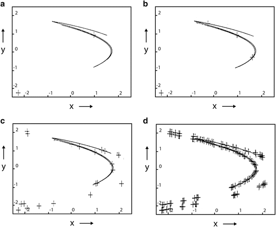

  

  Hénon strange chaotic attractor and periodic points of Hénon mapping (marked with crosses) with the following periods: (a) 1, (b) 1, 2, (c) 1, 2, 5, (d) 1, 2, 5, 10

• 2. The next example involves a bifurcation curve. On the vertical axis we put the parameter b, while on the horizontal axis x. In fact, it is the mapping of the family of attractors depending on the parameter b in the plane (b, x), 0. 1 ≤ b ≤ 0. 3 (see Fig. 15.19). For r = 1. 3 the chaotic dynamic of mapping is interrupted windows of periodicity for some values of b (there are infinitely many of them), however when reducing of the r and b ≈ 0. 26 bifurcation occurs, chaotic motion disappears and periodic motion appears. Then, each of the “branches” doubles and with further reduction of b formed are the so-called bubbles of chaotic motion (Fig. 15.19b).

  Fig. 15.19

  

  Bifurcation curve of the Hénon map and the parameters (a) r = 1. 3; (b) r = 1. 25

• 3. Basing on Hénon map we will discuss the concept of attractor attraction pools. By the attractor attraction pool will be defined the set of all initial conditions in phase space, which will be “attracted” by the attractor, that is after “start” of each of these initial conditions trajectories over time will be on the attractor. These pools of attraction for the Hénon mapping are shown in Fig. 15.20. For a set of parameters, as shown, there are three different attractors. One of them is ∞ (black area), stable periodic orbit with a period of eight (a gray area), and a strange chaotic attractor, in the figure consisting of two parts, which “attracts” the initial conditions from the white area.

  Fig. 15.20

  

  Pools of attraction for the Hénon map and for a = 1, r = 1, b = 0. 48

• 4. Now we will discuss the puzzling similarities between the Hénon attractor and the unstable variety of the fixed point lying within the attractor. Through a stable variety of the mapping fixed point we understand a set of points leading up to this point with the number of iterations tending to infinity defining the Hénon map. However, the concept of unstable variety of the mapping fixed point we mean a set of points which are attracted by the iterations with the opposite direction (or repelled by applying the initial iterations). Figure 15.21a shows the Hénon chaotic attractor, while Fig. 15.21b shows the set of points attracted by the reverse iteration by an unstable fixed point with coordinates (0. 855, 0. 898). It is striking similarity here between the two sets. It is believed that these sets are identical, but has not been proofed as accurate (see for example [219]).

  Fig. 15.21

  

  Hénon attractor for a = 1, r = 1. 38 and b = 0. 32 (a) and unstable variety of the fixed point with coordinates (x, y) = (0. 855, 0. 898) (b)

• 5. Now we will turn our attention to the similarity between the Hénon attractor attraction pool and attractor which is infinity (∞) (this will be a set of points that the iterations tending to infinity “escape” to infinity (Fig. 15.22a)), and a stable fixed point attraction pool within the Hénon attractor (Fig. 15.22b). The calculations were performed assuming the parameters: a = 1, $b = -0.32$, r = 2. 10. You can see that approximately the pool of attraction of a stable point of the Hénon attractor fits in the Hénon chaotic attractor attraction pool.

  Fig. 15.22

  

  Attraction pool for infinity (∞), marked with a black and the Hénon attractor attraction pool (a) and attracting pool of stable fixed point lying within the Hénon map, which is approximately (0.907, 0.966) (b). In both figures (a) and (b) marked is also Hénon attractor

• 6. There is also the possibility of the chaotic trajectory contained in a limited area in the phased space, however all other trajectories situated in the neighbourhood “escape” to infinity, so they are not bounded. Such invariant set will be called Hénon mapping chaotic saddle. This invariant and compact set is unstable, so almost all trajectories of the neighbourhood will be distancing themselves, and in the considered case, they will “escape” to infinity.

  Figure 15.23 shows an example of an unstable set that is invariant and compact, on which lays the chaotic trajectory. Calculations were performed for a = 1, b = 0. 4 and r = 4.

  Fig. 15.23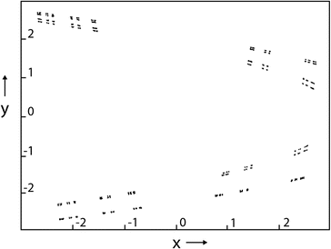

  

  Unstable invariant set containing a chaotic trajectory for Hénon map

• 7. From Fig. 15.23 we can conclude that for certain Hénon map parameters, there are two attractors which are attracting sets of the initial conditions. The first one is a pool of initial conditions attracted by Hénon chaotic attractor, and the second is a pool of initial conditions that in time are “fleeing” to infinity, or are attracted by infinity. There are also points belonging to the boundaries of the two pools, and the initial conditions are not attracted by any of these attractors [184]. This limited trajectory is shown in Fig. 15.24 for a = 1, $b = -0.3$, r = 2. 12.

  Fig. 15.24

  

  Border trajectory (marked with crosses) belonging to the boundaries of the Hénon attractor attraction pools (marked with points) and attractor lying in an “infinity”

• 8. In this example, basing on the Hénon map illustrated is a way leading to chaos by doubling of the period. The calculation results are shown in Fig. 15.25a–c.

  Fig. 15.25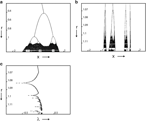

  

  Bifurcation graph illustrating the period doubling cascade leading to chaos (a) of the graph window (a) for 1. 06 ≤ r ≤ 1. 12 (b) and the Lyapunov exponent corresponding (b) to the figure (c)

  In the first one you can see the way that leads to chaotic motion by successive doubling period of vibration. Basing on Fig. 15.25a, b can be calculated the relations between lengths of the subsequent curves in between the points of the bifurcation, which are: $d_{2}/d_{4} = 4.33$, $d_{4}/d_{8} = 4.42$, $d_{8}/d_{16} = 4.54$ and apparently they tend to the Feigenbaum constant (approximately 4.67). Figure 15.25c shows the graph of changes in Lyapunov exponent λ in relation to Fig. 15.23b, that is for the same range of changes in parameter r. Where it is positive, there is chaos.

15.6.7 Ikeda Map

Ikeda map is described by the equation

$$\displaystyle{ z \rightarrow \rho +c_{2}z\exp \left [i\left (c_{1} - c_{3}\left (1 + z^{2}\right )^{-1}\right )\right ],\quad z = x + iy,x,y \in R,i^{2} = -1. }$$

(15.101)

Figure 15.26 shows three successive iterations of an ellipse located in the upper right-hand corners of the pictures for the following parameters: ρ = 0. 5, c ₁ = 0. 4, c ₂ = 0. 9, c ₃ = 6. Chaotic dynamic is more visible with each of the iterations.

Fig. 15.26

The first (a), second (b) and third (c) iteration of the ellipse shown in the upper right corners of the drawing for mapping Ikeda

Let us now consider the dynamics of Ikeda map (15.101) for the same parameters as before, but now iterated ellipse is shifted to the left compared to the one in the previous case (Fig. 15.27). As can be seen from this figure chaotic dynamics is revealed here much earlier.

Fig. 15.27

The first (a) and second (b) iteration of the ellipse for the Ikeda map

Figure 15.28 presented is only the first iteration of the ellipse, but in this case it is lying along the y = 0. 5 and for different values of the control parameter ρ. Increase of parameter ρ from 0.5 to 1.0 affects the deepening of the dynamics of Ikeda chaotic mappings.

Fig. 15.28

The first iteration of the ellipse for different values of the parameter ρ: (a) 0.6; (b) 0.7; (c) 0.8; (d) 0.9; (e) 1

15.7 Modelling of Nonlinear Ordinary Differential Equations

15.7.1 Introduction

In order to determine time evolution of the natural processes we should have the knowledge of the functional dependencies between the function that describes this process and its derivative (or derivatives) and in addition we have to know the initial conditions. As it has been already mentioned, the relationship between an unknown function and its derivative is called a differential equation. Nowadays it is very difficult to imagine the development in many fields of science without knowledge of the differential equations theory. There are many directions of development in modern theory of differential equations and various methods of teaching depending on the needs of the designated public. This section deals only with a few examples of systems of differential equations describing the dynamics of simple physical systems in terms of chaotic dynamics (see also the monograph [224]).

15.7.2 Non-autonomous Oscillator with Different Potentials

Imagine that ball (material point) is in the vessel with the cross-section indicated in Fig. 15.29.

Fig. 15.29

Ball movement in the vessel along the potential V (y)

The equation of the ball motion is:

$$\displaystyle{ \ddot{y} + c\dot{y} + \frac{dV \left (y\right )} {dy} = F\cos \omega t. }$$

(15.102)

The potential of V (y) may have two minima and one maximum, as is shown in Fig. 15.29, or it may assume other shapes (Fig. 15.30).

Fig. 15.30

Typical shapes of the potential V (y)

If we describe the potential with equation

$$\displaystyle{ V \left (y\right ) = \frac{\alpha y^{2}} {2} + \frac{\beta y^{4}} {4}, }$$

(15.103)

the case of Fig. 15.29 corresponds to the potential of α < 0 and β > 0, and for the potential of Fig. 15.30a we have α > 0 and β > 0, and for the potential shown in Fig. 15.30b we have α > 0 and β < 0.

Consider first the case of the system with no force and no damping. Then the dynamics of the system is described by the equations

$$\displaystyle\begin{array}{rcl} \dot{y}& =& x, \\ \dot{x}& =& -\alpha y -\beta y^{3}.{}\end{array}$$

(15.104)

Let us find a balance ball positions. In this case from $\dot{y} =\dot{ x} = 0$ and Eq. (15.104), we obtain

$$\displaystyle\begin{array}{rcl} x& =& 0, \\ y\left (\alpha +\beta y^{2}\right )& =& 0,{}\end{array}$$

(15.105)

which allows you to find three equilibrium positions (y ₀, x ₀) = (0, 0) and $\left (x_{0},y_{0}\right ) = \left (\pm \sqrt{\frac{-\alpha } {\beta }},0\right )$. Let us examine the stability of each of the found balance positions. For this purpose, assume that δ _x and δ _y are small perturbations respectively for x ₀ and y ₀, and we have

$$\displaystyle{ \begin{array}{c} x = x_{0} +\delta x, \\ y = y_{0} +\delta y, \end{array} }$$

(15.106)

which together with (15.104) leads after the linearization (that is leaving only the linear segments because of δ _x and δ _y ) of the equations

$$\displaystyle\begin{array}{rcl} \delta \dot{y}& =& +\delta x, \\ \delta \dot{x}& =& -\alpha \delta y - 3\beta y_{0}^{2}\delta y.{}\end{array}$$

(15.107)

We will look for solutions of (15.107) in the following form:

$$\displaystyle{ \begin{array}{c} \delta x = Xe^{\lambda t}, \\ \delta y = Y e^{\lambda t},\end{array} }$$

(15.108)

what after substituting into (15.107) yields the characteristic equation

$$\displaystyle{ \left \vert \begin{array}{cc} -1& \lambda \\ \lambda &\alpha +3\beta y_{ 0}^{2} \end{array} \right \vert = 0, }$$

(15.109)

from which we determine the following roots

$$\displaystyle{ \lambda _{1,2} = \pm \sqrt{-\alpha - 3\beta y_{0 }^{2}}. }$$

(15.110)

Next let us consider the case shown in Fig. 15.31. Then for (0,0) we have $\lambda _{1,2} = \pm \sqrt{-\alpha }$, and since α < 0, the roots are real and of opposite signs. Location (0,0) is a saddle. Two remaining equilibrium positions correspond to the eigenvalues

$$\displaystyle{ \lambda _{1,2} = \pm i\sqrt{-2\alpha }, }$$

(15.111)

that are imaginary values. Those positions of equilibrium are variety points of middle type. Location (0,0) is called hyperbolic, and the remaining equilibrium positions are elliptic. Phase trajectories with three equilibria are shown in Fig. 15.31.

Particularly noteworthy are two phase trajectories the shape of loop locked into eight. Trajectories coming out of the saddle-point 0 and returning to it is called the homoclinic trajectory (orbit). Homoclinic orbits can be described analytically in the form of the following two equations

$$\displaystyle\begin{array}{rcl} y_{H}\left (t\right )& =& \sqrt{\frac{-2\alpha } {\beta }} \sec h\left (\pm \sqrt{-\alpha }\left (t - t_{0}\right )\right ), \\ x_{H}\left (t\right )& =& -\alpha \sqrt{\frac{2} {\beta }} \sec h\left (\pm \sqrt{-\alpha }\left (t - t_{0}\right )\right )\mbox{ tanh}\left (\pm \sqrt{-\alpha }\left (t - t_{0}\right )\right ),{}\end{array}$$

(15.112)

where t is the time parameter.

Fig. 15.31

Three equilibria and the surrounding them phase trajectories

15.7.3 Melnikov Function and Chaos

The basic idea of the Melnikov method [22, 106] is to use a solution of the uninterrupted integrable system of two differential equations to solve the disturbed system of equations. Let the dynamics of the system to be described by the equations:

$$\displaystyle\begin{array}{rcl} \dot{x}& =& f_{1}\left (x,y\right ) +\varepsilon g_{1}\left (x,y,t\right ), \\ \dot{y}& =& f_{2}\left (x,y\right ) +\varepsilon g_{2}\left (x,y,t\right ){}\end{array}$$

(15.113)

Parameter $\varepsilon > 0$ is a value $\varepsilon \ll 1$ and is called the small perturbation parameter. It emphasizes the “smallness” of time-dependent disorders g _i (i = 1, 2). In such a system chaotic motion may appear, and a set of parameters for which it appears can be determined with the method described below.

For $\varepsilon = 0$ undisturbed system has two homoclinic orbits H ⁰(t) to the saddle point (0,0). The core of homoclinic orbits is filled with one-parameter family of periodic orbits H ^γ(t) with period T ^γ dependent on parameter γ ∈ (1, 0)—see Fig. 15.31.

If in the system (15.113) forcing functions g _i (i = 1, 2) are periodic in time, while the functions f _i (i = 1, 2) have homoclinic orbit (as in Fig. 15.31), then the Melnikov function as follows

$$\displaystyle\begin{array}{rcl} M\left (t_{0}\right )& =& \varepsilon \int _{-\infty }^{\infty }\left \{\left (f_{ 1}\left [x_{H^{0}\left (t-t_{0}\right )},\,y_{H^{0}\left (t-t_{0}\right )}\right ]g_{2}\left [x_{H^{0}\left (t-t_{0}\right )},\,y_{H^{0}\left (t-t_{0}\right )},\,t\right ]\right )\right. \\ & & -\left.f_{2}\left [x_{H^{0}\left (t-t_{0}\right )},\,y_{H^{0}\left (t-t_{0}\right )}\right ]g_{1}\left [x_{H^{0}\left (t-t_{0}\right )},\,y_{H^{0}\left (t-t_{0}\right )},\,t\right ]\right \}dt.{}\end{array}$$

(15.114)

If the function M(t ₀) does not yield zero values, then the stable and unstable manifolds do not intersect anywhere beyond the saddle point. If the equation M(t ₀) = 0 has a solution, then additional intersection occurs. Let us now return to Eq. (15.102) and potential (15.103).

The equation of motion of the oscillator with such a choice of the potential takes the form

$$\displaystyle\begin{array}{rcl} \dot{y}& =& x, \\ \dot{x}& =& -\alpha y -\beta y^{3} -\varepsilon cx +\varepsilon F\cos \omega t,{}\end{array}$$

(15.115)

where $\varepsilon$ c and $\varepsilon$ F highlight the “smallness” of the distinguished parameters.

Assuming

$$\displaystyle\begin{array}{rcl} f_{1}& =& x,\quad f_{2} = -\alpha y -\beta y^{3}, \\ g_{1}& =& 0,\quad g_{2} = \epsilon (F\cos \omega t - cx),{}\end{array}$$

(15.116)

and using (15.114), we obtain

$$\displaystyle{ M\left (t_{0}\right ) = \frac{4c\sqrt{\left (-\alpha \right ) ^{3}}} {3\beta } +\pi F\omega \sqrt{\frac{2} {\beta }} \frac{\sin \omega t_{0}} {\cosh \frac{\pi \omega } {2\sqrt{-\alpha }}}. }$$

(15.117)

The function M(t ₀) changes sign for the following relationship between the parameters

$$\displaystyle{ F = \frac{4c\sqrt{\left (-\alpha \right ) ^{3}}} {3\pi \omega \sqrt{2\beta }} \cosh \left [ \frac{\pi \omega } {2\sqrt{-\alpha }}\right ]. }$$

(15.118)

Let us take into consideration the following parameters: c = 0. 8, $\alpha = -12$, β = 100, ω = 3. 3. The value of the last parameter is calculated from the formula (15.118) obtaining F = 1. 3295. Equations (15.115) for given parameters were solved numerically and the numerical simulation results are shown in Fig. 15.32.

The phase trajectory “jumps” in a random way between two points corresponding to a minimum of two wells of the potential V (y). Figure 15.32b shows the strange chaotic attractor on the plane in the form of an infinite set of points, while the distance in time between two successive points is $T = 2\pi /\omega$ (the Poincaré map).

Fig. 15.32

Phase trajectory (a) and Poincaré map (b) for the Duffing oscillator governed by Eq. (15.115)

In Fig. 15.33 as a control parameter taken was the amplitude of the exciting force F (other parameters unchanged) and plotted the maximum value of the Lyapunov exponent for 1 ≤ F ≤ 2. You can see that chaos appears for F = 1. 33, and then disappears in the vicinity of $F\mathop{\cong}1.62$.

Fig. 15.33

Changes of Lyapunov exponent as a function of the parameter F

Fig. 15.34

Strange chaotic attractor discovered by Ueda

Consider the case of the potential when α = 0 and β > 0. This case was analysed by Ueda [233]. Presented strange chaotic attractor is often referred to as Japanese attractor.

Vibrations of many simple physical systems can be simplified to the Duffing equation. The equation of motion of the plane pendulum of inertia mass moment equal B = ml ², with air resistance coefficient c forced by the moment M = M ₁cosω t has the form (see Fig. 15.34)

$$\displaystyle{ B\ddot{\varphi } = -mgl\sin \varphi - c_{0}\dot{\varphi } + M_{1}\cos \omega t. }$$

(15.119)

After dividing by B we get

$$\displaystyle{ \ddot{\varphi }+c\dot{\varphi }+\beta \sin \varphi = F\cos \omega t, }$$

(15.120)

where: $c = c_{0}/B$, $\beta = mgl/B$, $F = M_{1}/B$.

Chaotic dynamics of the pendulum takes a place for ω = 1, F = 2. 4, c = 0. 2, β = 1.

15.7.4 Lorenz Attractor

Lorenz model is a system of three nonlinear ordinary differential equations of the first order [157]. Now we will derive those equations basing on the old problem of Rayleigh–Benard (reading of this induction of equations process can be omitted without problems in further analysis of the chaotic dynamics).

Fig. 15.35

Scheme of the process of Rayleigh–Benard convection used to derive equations Lorenz

Let between two infinitely long plates with H distance be a liquid (Fig. 15.35). The liquid is heated from the bottom. Let u to be the velocity of liquid particles, let T _s to be the temperature surface, ρ _s to be density surface and pressure p _s , where T ₀ corresponds ρ ₀ and g is the acceleration due to gravity. Temperature, pressure and density are changed according to the following formulas (for u = 0), $\Delta T$ is the linear increase of the temperature.

$$\displaystyle\begin{array}{rcl} T_{s}(z)& =& T_{0} + \Delta T -\left ( \frac{z} {H}\right )\Delta T, \\ \rho _{s}(z)& =& \rho _{0}[1 -\alpha (T_{s}(z) - T_{0})], \\ \nabla p_{s}(z)& =& -\rho _{s}(z)g\bar{z}, {}\end{array}$$

(15.121)

where $\bar{z}$ is the normal vector in the z direction. Firstly (that is with the provision of the low thermal energy) occurs laminar convection. Subsequently, stable vortices are formed, wherein the temperature increase is nonlinear described by

$$\displaystyle{ \Theta \left (x,y,z,t\right ) = T\left (x,y,z,t\right ) - T_{s}\left (z\right ). }$$

(15.122)

Speed u changes in time and the dynamics of the flow is described following system of partial differential equations

$$\displaystyle\begin{array}{rcl} \frac{\partial u} {\partial t} + \left (u \cdot \nabla \right )u& =& \alpha \Theta g\bar{z} -\left (\frac{1} {\rho _{0}} \right )\nabla \delta p +\nu \nabla ^{2}u, \\ \frac{\partial \Theta } {\partial t} + \left (u \cdot \nabla \right )\Theta & =& \chi \nabla ^{2}\Theta - u_{ z}\left (\frac{\Delta T} {H} \right ), \\ \nabla u& =& 0. {}\end{array}$$

(15.123)

Here δ p is the pressure change proportional to the convection state, ν is the liquid kinetic viscosity coefficient, χ is a constant thermal diffusion process, and ∇² is the Laplace operator. Since u _y  = 0, then the remaining components of the velocity vector can be obtained from the equations:

$$\displaystyle{ u_{x} = -\frac{\partial \psi } {\partial z},\quad u_{z} = \frac{\partial \psi } {\partial x}. }$$

(15.124)

In addition, Lorenz introduced the following boundary conditions:

$$\displaystyle{ \Theta \left (0\right ) = \Theta \left (H\right ) =\psi \left (0\right ) =\psi \left (H\right ) = \nabla ^{2}\psi \left (0\right ) = \nabla ^{2}\psi \left (H\right ) = 0. }$$

(15.125)

Function of temperature dispersion $\Theta$ and flow function ψ can be found in the form of the following Fourier series:

$$\displaystyle{ \begin{array}{c} \Theta \left (x,y,z,t\right ) =\sum _{ j=1}^{J}\sin \left (j\pi z\right )\Theta _{j}\left (x,t\right ), \\ \psi \left (x,y,z,t\right ) =\sum _{ j=1}^{J}\sin \left (j\pi z\right )\psi _{j}\left (x,t\right ).\end{array} }$$

(15.126)

Further Lorenz limited his considerations to only three basic solutions, and taking into account the boundary conditions he obtained

$$\displaystyle\begin{array}{rcl} \Theta \left (x,z,t\right )& =& \frac{\Delta TR_{c}} {R_{a}\pi } \left [\sqrt{2}Y \left (t\right )\cos \left (\frac{\pi ax} {H} \right )\sin \left ( \frac{\pi z} {H}\right ) - z\left (t\right )\sin \left (\frac{2\pi z} {H}\right )\right ], \\ \psi \left (x,z,t\right )& =& \frac{\sqrt{2}\left (1 + a^{2}\right )\chi } {a} X\left (t\right )\sin \left (\frac{\pi ax} {H} \right )\sin \left ( \frac{\pi z} {H}\right ), {}\end{array}$$

(15.127)

where R _a is the Rayleigh number with the critical value R _c :

$$\displaystyle{ R_{a} = \frac{\alpha gH^{3}\Delta T} {\chi \nu },\quad R_{c} = \frac{\pi ^{4}\left (1 + a^{2}\right )^{3}} {a^{2}}. }$$

(15.128)

X, Z and Z are amplitudes of three successive forms of the assumed solution that are dependent on time. Lorenz equations we obtain by substituting (15.127) into Eq. (15.123). They have the following form

$$\displaystyle\begin{array}{rcl} \frac{dX} {d\tau } & =& \sigma \left (Y - X\right ), \\ \frac{dY } {d\tau } & =& -XZ + rX - Y, \\ \frac{dZ} {d\tau } & =& XY - bZ, {}\end{array}$$

(15.129)

where

$$\displaystyle{ \tau = \frac{\pi \left (1 + a^{2}\right )\chi t} {\chi ^{2}},\quad \sigma = \frac{\mu } {\chi },\quad b = \frac{4} {1 + a^{2}},\quad r = \frac{R_{a}} {R_{c}}. }$$

(15.130)

During computer simulations of these equations Lorenz noticed irregular oscillations for certain parameters of this strongly simplified version of a physical model. He also noted in the plane (X, Y ) a geometric shape somewhat resembling a human kidney. Phase point wandered around the left or right kidney, while the jumps between them were random and impossible to predict.

Lorenz equations system is an autonomous system (without acting external force). Let us try to determine the equilibrium position of the system and investigate their stability. For b > 0, σ > 0 and r > 0, Eq. (15.129), we obtain

$$\displaystyle\begin{array}{rcl} \sigma \left (Y - Z\right )& =& 0, \\ -XY + rX - Y & =& 0, \\ XY - bZ& =& 0.{}\end{array}$$

(15.131)

As one can easily verify (X, Y, Z) = (0, 0, 0). Disturbing the equilibrium position and limiting the discussion to the differential equations of the linear disorders we obtain the characteristic equation of the form

$$\displaystyle{ \left [\lambda +b\right ]\left [\lambda ^{2} + \left (\sigma +1\right )\lambda +\sigma \left (1 - r\right )\right ] = 0. }$$

(15.132)

Fig. 15.36

Lorenz attractor projection on the plane (X, Y ) for σ = 10, r = 28, b = 2. 67

For 0 < r < 1 Eq. (15.132) has three real roots neither of which is negative. This means that considered equilibrium position is a stable. For r = 1 occurs solutions branching–bifurcation. For r > 1 we have the following solution set (the equilibrium)

$$\displaystyle\begin{array}{rcl} X& =& Y = \pm \sqrt{b\left (r - 1 \right )}, \\ Z& =& r - 1. {}\end{array}$$

(15.133)

The previous solution (0,0,0) still exists, but is unstable. Characteristic equation in the considered case takes the form

$$\displaystyle{ \lambda ^{3} + \left (\sigma +b + 1\right )\lambda ^{2} + \left (r+\sigma \right )b\lambda + 2\sigma b\left (r - 1\right ) = 0. }$$

(15.134)

Both the equilibrium positions defined by Eq. (15.133) lose their stability after exceeding the critical value of the parameter.

$$\displaystyle{ r_{c} = \frac{\sigma \left (\sigma +b + 3\right )} {\sigma -b - 1}. }$$

(15.135)

Lorenz attractor projection is shown in Fig. 15.36. Numerically calculated attractor dimension equals d = 1. 768 ± 0. 071. Figure 15.37 shows a graph of the Lyapunov exponent λ in dependence of the control parameter r. For big values it assumes positive values, what reflects the chaotic traffic.

Fig. 15.37

λ Lyapunov exponent as a function of the parameter r

Fig. 15.38

The ith triple pendulum (a) and example of three coupled sets of pendulums (b)

15.8 Synchronization Phenomena of Coupled Triple Pendulums

15.8.1 Mathematical Model

The investigated system consists of N identical triple pendulums [27]. Each triple pendulum, exhibited in Fig. 15.38a is a plane subsystem of three rigid links, rotationally coupled in points O _j (j = 1, 2, 3), with viscous damping of the coefficients $\bar{c}_{j}$ (i = 1, 2, …, N), respectively. The position of the system is defined by 3N angles ψ _i, j $(i = 1,2,\ldots,N,\,\,j = 1,2,3)$. Masses of the corresponding links are denoted by m _j (j = 1, 2, 3), while I _j denote mass moments of inertia of the corresponding bodies with respect to axes z _cj (j = 1, 2, 3) - principal central axes perpendicular to the motion plane. It is assumed that the mass centers (axes z _cj ) of the links lie on the lines including the corresponding joints (O _j , j = 1, 2, 3). The first link of each pendulum is forced by the external and common signal $\varphi \left (\tau \right ) =\bar{\omega }\tau$ (where τ is time), realized by relative rotation of additional body (of mass m ₀ and inertia moment I ₀) connected to the first link in the joint O ₁. Other geometric parameters of the system are visible in Fig. 15.38a. The pendulum sets are situated along a line perpendicular to the motion plane and they are coupled by viscous and elastic connections (with angular viscous damping coefficient $\bar{k}_{s}\bar{c}_{rs}$ and angular stiffness $\bar{k}_{s}$) between the first links of neighbouring sets of triple pendulums. Figure 15.38b exhibits an example of three coupled sets of triple pendulums.

The system is governed by the following set of differential equations in the Lagrange formalism

$$\displaystyle{ \frac{d} {d\tau }\left ( \frac{\partial \bar{T}_{i}} {\partial {\mathop{\psi }\limits^{\vert }}_{i,j}}\right ) -\frac{\partial \bar{T}_{i}} {\partial \psi _{i,j}} + \frac{\partial \bar{V }_{i}} {\partial \psi _{i,j}} =\bar{ Q}_{i,j}\quad i = 1,\ldots,N,\quad j = 1,2,3, }$$

(15.136)

where $\mathop{(\ldots )}\limits^{\vert }$—denotes derivative with respect to real time $\tau,\bar{T}_{i},\bar{V }_{i}$—real kinetic and potential energy of the ith pendulum, $\bar{Q}_{i,j}$—real generalized forces acting in the system. The reader may find more material devoted to numerical and experimental investigations of the triple pendulum set in [27, 28, 36].

Real kinetic energy of the ith pendulum follows

$$\displaystyle\begin{array}{rcl} \bar{T}_{i}& =& A_{i}({\mathop{\psi }\limits^{\vert }}_{i,1}) + \frac{1} {2}B_{1}{\mathop{\psi ^{2}}\limits^{\vert }}_{ i,1} + \frac{1} {2}B_{2}{\mathop{\psi ^{2}}\limits^{\vert }}_{ i,2} + \frac{1} {2}B_{3}{\mathop{\psi ^{2}}\limits^{\vert }}_{ i,3} \\ & & +N_{12}{\mathop{\psi }\limits^{\vert }}_{i,1}{\mathop{\psi }\limits^{\vert }}_{i,2}\cos \left (\psi _{i,1} -\psi _{i,2}\right ) + N_{13}{\mathop{\psi }\limits^{\vert }}_{i,1}{\mathop{\psi }\limits^{\vert }}_{i,3}\cos \left (\psi _{i,1} -\psi _{i,3}\right ) \\ & & +N_{23}{\mathop{\psi }\limits^{\vert }}_{i,2}{\mathop{\psi }\limits^{\vert }}_{i,3}\cos \left (\psi _{i,2} -\psi _{i,3}\right ) {}\end{array}$$

(15.137)

where:

$$\displaystyle\begin{array}{rcl} B_{1}& =& I_{0} + I_{1} + e_{1}^{2}m_{ 1} + e_{0}^{2}m_{ 0} + l_{1}^{2}\left (m_{ 2} + m_{3}\right ), \\ B_{2}& =& I_{2} + e_{2}^{2}m_{ 2} + l_{2}^{2}m_{ 3}, \\ B_{3}& =& I_{3} + e_{3}^{2}m_{ 3}, \\ N_{12}& =& m_{2}e_{2}l_{1} + m_{3}l_{1}l_{2}, \\ N_{13}& =& m_{3}e_{3}l_{1}, \\ N_{23}& =& m_{3}e_{3}l_{2}, {}\end{array}$$

(15.138)

and where

$$\displaystyle{ A_{i}({\mathop{\psi }\limits^{\vert }}_{i,1}) = \frac{1} {2}\bar{\omega }_{i}\left [I_{0}\left (\bar{\omega }_{i} - 2{\mathop{\psi }\limits^{\vert }}_{i,1}\right ) + e_{0}^{2}m_{ 0}\left (\bar{\omega }_{i} + 2{\mathop{\psi }\limits^{\vert }}_{i,1}\right )\right ]. }$$

(15.139)

Real potential energy of gravitational forces for the i-th pendulum is as follows

$$\displaystyle{ \bar{V }_{i} = -M_{0}\cos \left (\psi _{i,1} +\bar{\omega } _{i}\tau \right ) - M_{1}\cos \psi _{i,1} - M_{2}\cos \psi _{i,2} - M_{3}\cos \psi _{i,3}, }$$

(15.140)

where

$$\displaystyle{ \begin{array}{c} M_{0} = m_{0}g\,e_{0},\quad M_{1} = m_{1}g\,e_{1} + \left (m_{2} + m_{3}\right )g\,l_{1}, \\ M_{2} = m_{2}g\,e_{2} + m_{3}g\,l_{2},\quad M_{3} = m_{3}g\,e_{3}, \end{array} }$$

(15.141)

and g is the gravitational acceleration.

The coupling between the adjacent sets of triple pendulums is modelled by following generalized forces

$$\displaystyle\begin{array}{rcl} \bar{Q}_{i,1}& =& -\bar{c}_{1}{\mathop{\psi }\limits^{\vert }}_{i,1} -\bar{ c}_{2}\left ({\mathop{\psi }\limits^{\vert }}_{i,1} -{\mathop{\psi }\limits^{\vert }}_{i,2}\right ) \\ & & + -\bar{ k}_{s}\left [\left (\psi _{i+1,1} -\psi _{i,1}\right ) + \left (\psi _{i-1,1} -\psi _{i,1}\right ) +\bar{ c}_{rs}\left ({\mathop{\psi }\limits^{\vert }}_{i+1,1} -{\mathop{\psi }\limits^{\vert }}_{i,1}\right )\right. \\ & & \left.+\bar{c}_{rs}\left ({\mathop{\psi }\limits^{\vert }}_{i-1,1} -{\mathop{\psi }\limits^{\vert }}_{i,1}\right )\right ], \\ \bar{Q}_{i,2}& =& -\bar{c}_{2}\left ({\mathop{\psi }\limits^{\vert }}_{i,2} -{\mathop{\psi }\limits^{\vert }}_{i,1}\right ) -\bar{ c}_{3}\left ({\mathop{\psi }\limits^{\vert }}_{i,2} -{\mathop{\psi }\limits^{\vert }}_{i,3}\right ), \\ \bar{Q}_{i,3}& =& -\bar{c}_{3}\left ({\mathop{\psi }\limits^{\vert }}_{i,3} -{\mathop{\psi }\limits^{\vert }}_{i,2}\right ),\quad \mathrm{where}\quad i =1,\ldots,N {}\end{array}$$

(15.142)

and where we assume that ψ _0, 1 = ψ _1, 1, ${\mathop{\psi }\limits^{\vert }}_{0,1} ={\mathop{\psi }\limits^{ \vert }}_{1,1}$, $\psi _{N+1,1} =\psi _{N,1}$, ${\mathop{\psi }\limits^{\vert }}_{N+1,1} ={\mathop{\psi }\limits^{ \vert }}_{N,1}$.

Then we introduce the non-dimensional time t

$$\displaystyle{ t =\alpha _{1}\tau, }$$

(15.143)

where

$$\displaystyle{ \alpha _{1} = \left (M_{1}B_{1}^{-1}\right )^{\frac{1} {2} }. }$$

(15.144)

Furthermore, we take

$$\displaystyle{ \frac{d\left (\ldots \right )} {d\tau } =\alpha _{1}\frac{d\left (\ldots \right )} {dt} }$$

(15.145)

and therefore

$$\displaystyle{ \begin{array}{c} {\mathop{\psi }\limits^{\vert }}_{i,j} =\alpha _{1}\dot{\psi }_{i,j},\\ \bar{\omega } =\alpha _{ 1}\omega, \\ \frac{\partial \left (\ldots \right )} {\partial {\mathop{\psi }\limits^{\vert }}_{i,j}} = \frac{\partial \left (\ldots \right )} {\partial \dot{\psi }_{i,j}} \frac{\partial \dot{\psi }_{i,j}({\mathop{\psi }\limits^{\vert }}_{j})} {\partial {\mathop{\psi }\limits^{\vert }}_{i,j}} = \frac{1} {\alpha _{1}} \frac{\partial \left (\ldots \right )} {\partial \dot{\psi }_{j}}, \end{array} }$$

(15.146)

where i = 1, …, N, j = 1, 2, 3, ω denotes the non-dimensional counterpart of real angular frequency $\bar{\omega }$ and (…) is derivative with respect to non-dimensional time t.

Dividing both sides of the real equations (15.136) by 2E ₁, where

$$\displaystyle{ E_{1} = \frac{1} {2}\alpha _{1}^{2}B_{ 1} = \frac{1} {2}M_{1}, }$$

(15.147)

the following non-dimensional Lagrange formulation of the governing equations is obtained

$$\displaystyle{ \frac{d} {dt}\left (\frac{\partial T_{i}} {\partial \dot{\psi }_{i,j}} \right ) -\frac{\partial T_{i}} {\partial \psi _{i,j}} + \frac{\partial V _{i}} {\partial \psi _{i,j}} = Q_{i,j},\quad i = 1,\ldots,N\quad j = 1,2,3. }$$

(15.148)

Non-dimensional kinetic energy of the i-th pendulum is as follows

$$\displaystyle\begin{array}{rcl} T_{i}& =& \frac{\bar{T}_{i}} {2E_{1}} = a_{i}(\dot{\psi }_{i,1}) + \frac{1} {2}\dot{\psi }_{i,1}^{2} + \frac{1} {2}\beta _{2}\dot{\psi }_{i,2}^{2} + \frac{1} {2}\beta _{3}\dot{\psi }_{i,3}^{2} \\ & & +\nu _{12}\dot{\psi }_{i,1}\dot{\psi }_{i,2}\cos \left (\psi _{i,1} -\psi _{i,2}\right ) +\nu _{13}\dot{\psi }_{i,1}\dot{\psi }_{i,3}\cos \left (\psi _{i,1} -\psi _{i,3}\right ) \\ & & +\nu _{23}\dot{\psi }_{i,2}\dot{\psi }_{i,3}\cos \left (\psi _{i,2} -\psi _{i,3}\right ) {}\end{array}$$

(15.149)

where

$$\displaystyle{ \beta _{2} = \frac{B_{2}} {B_{1}},\beta _{3} = \frac{B_{3}} {B_{1}},\nu _{12} = \frac{N_{12}} {B_{1}},\nu _{13} = \frac{N_{13}} {B_{1}}, }$$

(15.150)

and

$$\displaystyle{ a_{i}(\dot{\psi }_{i,1}) = \frac{A_{i}({\mathop{\psi }\limits^{\vert }}_{i,1})} {2E_{1}} = \frac{1} {2B_{1}}\omega _{i}\left [I_{0}\left (\omega _{i} - 2\dot{\psi }_{i,1}\right ) + e_{0}^{2}m_{ 0}\left (\omega _{i} + 2\dot{\psi }_{i,1}\right )\right ]. }$$

(15.151)

Non-dimensional potential energy of gravitational forces for the i-th pendulum has the form

$$\displaystyle{ V _{i} = \frac{\bar{V }_{i}} {2E_{1}} = -\mu _{0}\cos \left (\psi _{i,1} +\omega _{i}t\right ) -\cos \psi _{i,1} -\mu _{2}\cos \psi _{i,2} -\mu _{3}\cos \psi _{i,3} }$$

(15.152)

where

$$\displaystyle{ \mu _{0} = \frac{M_{0}} {M_{1}},\mu _{2} = \frac{M_{2}} {M_{1}},\mu _{3} = \frac{M_{3}} {M_{1}}. }$$

(15.153)

Non-dimensional generalized forces have the following form

$$\displaystyle\begin{array}{rcl} Q_{i,1}& =& \frac{\bar{Q}_{i,1}} {2E_{1}} = -c_{1}\dot{\psi }_{i,1} - c_{2}\left (\dot{\psi }_{i,1} -\dot{\psi }_{i,2}\right ) \\ & & + - k_{s}\left [\left (\psi _{i+1,1} -\psi _{i,1}\right ) + \left (\psi _{i-1,1} -\psi _{i,1}\right ) + c_{rs}\left (\dot{\psi }_{i+1,1} -\dot{\psi }_{i,1}\right )\right. \\ & & \left.+c_{rs}\left (\dot{\psi }_{i-1,1} -\dot{\psi }_{i,1}\right )\right ], \\ Q_{i,2}& =& \frac{\bar{Q}_{i,2}} {2E_{1}} = -c_{2}\left (\dot{\psi }_{i,2} -\dot{\psi }_{i,1}\right ) - c_{3}\left (\dot{\psi }_{i,2} -\dot{\psi }_{i,3}\right ), \\ Q_{i,3}& =& \frac{\bar{Q}_{i,3}} {2E_{1}} = -c_{3}\left (\dot{\psi }_{i,3} -\dot{\psi }_{i,2}\right ),\quad i =1,2,\ldots,N, {}\end{array}$$

(15.154)

where

$$\displaystyle{ \begin{array}{c} c_{j} = \frac{\bar{c}_{j}} {\sqrt{M_{1 } B_{1}}},\quad \mathrm{for}\quad j = 1,2,3, \\ k_{s} = \frac{\bar{k}_{s}} {M_{1}},\quad c_{rs} =\bar{ c}_{rs}\sqrt{\frac{M_{1 } } {B_{1}}} \end{array} }$$

(15.155)

and where we take ψ _0, 1 = ψ _1, 1, $\dot{\psi }_{0,1} =\dot{\psi } _{1,1}$, $\psi _{N+1,1} =\psi _{N,1}$, $\dot{\psi }_{N+1,1} =\dot{\psi } _{N,1}$.

Finally, the non-dimensional governing equations can be written as follows

$$\displaystyle{ \begin{array}{c} \mathbf{M}\left (\boldsymbol{\psi }_{i}\right )\,\ddot{\boldsymbol{\psi }}_{i} + \mathbf{N}\left (\boldsymbol{\psi }_{i}\right )\,\dot{\boldsymbol{\psi }}_{i}^{2} + \mathbf{C}\,\dot{\boldsymbol{\psi }}_{i} + \mathbf{p}\left (\boldsymbol{\psi }_{i},t\right ) = \mathbf{f}\left (\boldsymbol{\psi }_{i-1},\boldsymbol{\psi }_{i},\boldsymbol{\psi }_{i+1},\dot{\boldsymbol{\psi }}_{i-1},\dot{\boldsymbol{\psi }}_{i},\dot{\boldsymbol{\psi }}_{i+1}\right ) \\ i =1,2,\ldots,N\end{array} }$$

(15.156)

where

$$\displaystyle\begin{array}{rcl} \boldsymbol{\psi }_{i}& =& \left \{\begin{array}{c} \psi _{i,1}^{} \\ \psi _{i,2}^{} \\ \psi _{i,3}^{}\end{array} \right \},\quad \dot{\boldsymbol{\psi }}_{i} = \left \{\begin{array}{c} \dot{\psi }_{i,1}^{} \\ \dot{\psi }_{i,2}^{} \\ \dot{\psi }_{i,3}^{}\end{array} \right \},\quad \dot{\boldsymbol{\psi }}_{i}^{2} = \left \{\begin{array}{c} \dot{\psi }_{i,1}^{2} \\ \dot{\psi }_{i,2}^{2} \\ \dot{\psi }_{i,3}^{2} \end{array} \right \},\quad \ddot{\boldsymbol{\psi }}_{i} = \left \{\begin{array}{c} \ddot{\psi }_{i,1} \\ \ddot{\psi }_{i,2} \\ \ddot{\psi }_{i,3}\end{array} \right \}, \\ \mathbf{M}\left (\boldsymbol{\psi }_{i}\right )& =& \left [\begin{array}{ccc} 1 &\nu _{12}\cos \left (\psi _{i,1} -\psi _{i,2}\right )&\nu _{13}\cos \left (\psi _{i,1} -\psi _{i,3}\right ) \\ \nu _{12}\cos \left (\psi _{i,1} -\psi _{i,2}\right )& \beta _{2} & \nu _{23}\cos \left (\psi _{i,2} -\psi _{i,3}\right ) \\ \nu _{13}\cos \left (\psi _{i,1} -\psi _{i,3}\right )&\nu _{23}\cos \left (\psi _{i,2} -\psi _{i,3}\right )& \beta _{3} \end{array} \right ], \\ \mathbf{N}\left (\boldsymbol{\psi }_{i}\right )& =& \left [\begin{array}{ccc} 0 & \nu _{12}\sin \left (\psi _{i,1} -\psi _{i,2}\right ) &\nu _{13}\sin \left (\psi _{i,1} -\psi _{i,3}\right ) \\ -\nu _{12}\sin \left (\psi _{i,1} -\psi _{i,2}\right )& 0 &\nu _{23}\sin \left (\psi _{i,2} -\psi _{i,3}\right ) \\ -\nu _{13}\sin \left (\psi _{i,1} -\psi _{i,3}\right )&-\nu _{23}\sin \left (\psi _{i,2} -\psi _{i,3}\right )& 0 \end{array} \right ], \\ \mathbf{C}& =& \left [\begin{array}{ccc} c_{1}+c_{2} & -c_{2} & 0 \\ -c_{2} & c_{2}+c_{3} & -c_{3} \\ 0 & -c_{3} & c_{3} \end{array} \right ],\quad \mathbf{p}\left (\psi _{i},t\right ) = \left \{\begin{array}{c} \sin \psi _{i,1}+\mu _{0}\sin \left (\psi _{i,1}+\omega t\right )\\ \mu _{ 2}\sin \psi _{i,2} \\ \mu _{2}\frac{\nu _{12}} {\nu _{13}} \sin \psi _{i,3} \end{array} \right \}, \\ \mathbf{f}& =& k_{s}\left \{\begin{array}{c} \psi _{i-1} - 2\psi _{i} +\psi _{i+1} + c_{rs}\left (\dot{\psi }_{i-1} - 2\dot{\psi }_{i} +\dot{\psi } _{i+1}\right ) \\ 0\\ 0 \end{array} \right \}. {}\end{array}$$

(15.157)

15.8.2 Numerical Simulations

The following set of real parameters is constant during the numerical simulations presented in the current section

$$\displaystyle\begin{array}{rcl} m_{0}& =& m_{1} = m_{2} = m_{3} = 1\,\mathrm{kg}, \\ I_{0}& =& I_{1} = I_{2} = I_{3} = \frac{1} {12}\,\mathrm{kg} \cdot \mathrm{m}^{\mathrm{2}}, \\ e_{1}& =& 0,\quad e_{0} = e_{2} = e_{3} = \frac{1} {2}\,\mathrm{m},\quad l_{1} = l_{2} = 1\,\mathrm{m}, \\ \bar{c}_{1}& =& \bar{c}_{2} =\bar{ c}_{3} = 0.1\,\mathrm{N}\,\mathrm{m}\,\mathrm{s},\quad \bar{c}_{rs} = 0.347611\,\mathrm{s},\quad g = 10\,\mathrm{m}/\mathrm{s}^{\mathrm{2}}.{}\end{array}$$

(15.158)

The set of real quantities (15.158) leads to the following non-dimensional parameters

$$\displaystyle\begin{array}{rcl} \beta _{2}& =& 0.5517,\quad \beta _{3} = 0.1379, \\ \mu _{0}& =& 0.25,\quad \mu _{2} = 0.75, \\ \nu _{23}& =& 0.2068,\quad \nu _{12} = 0.6207,\quad \nu _{13} = 0.2068, \\ c_{1}& =& c_{2} = c_{3} = 0.01438,\quad c_{rs} = \mathrm{1}.{}\end{array}$$

(15.159)

Fig. 15.39

Bifurcational diagram for one (N = 1) triple pendulum (a) and the corresponding periodic solution for ω = 0. 68 (b) and chaotic attractor for ω = 0. 72 [(c) trajectory, (d) Poincaré section]

Fig. 15.40

Bifurcational diagrams for three (N = 3) coupled triple pendulums

Figure 15.39a exhibits bifurcational diagram for one (N = 1) or for uncoupled triple pendulums (k _s  = 0), with the excitation angular frequency ω as a bifurcational parameter. In Fig 15.39b–d there are presented two exemplary orbits: the periodic (b) for ω = 0. 68 and the chaotic one for ω = 0. 72 (c, d). Then, for (chaotic behaviour of uncoupled systems), we present bifurcational diagrams (Fig. 15.40) of dynamical behaviour of three coupled pendulums (N = 3), with coupling coefficient k _s as a control parameter. The first Poincaré section (for k _s  = 0) of each bifurcational diagram is performed by the use of the following set of initial conditions

$$\displaystyle{ \psi _{i,j}(0) = 0,\quad \dot{\psi }_{i,j}(0) = 10^{-5}i\quad \mathrm{where}\quad i = 1,2,\ldots,N,\quad j = 1,2,3, }$$

(15.160)

so the pendulums start from closely located, but different states. During a jump to the next Poincaré section (the change of control parameter), see Fig. 15.40a, the system state preserves continuity or is restarted to the initial conditions (15.160)—see Fig. 15.40b. Figure 15.40 exhibits rich spectrum of synchronization phenomena governed by the investigated system (the associated Poincaré maps are reported in Fig. 15.41). In particular, we have observed the intervals of chaotic and periodic behaviour of the system, or even regions of coexistence of chaotic and periodic attractors. We have also found the intervals of exact synchronization between chaotic behaviour of all three pendulums and the zones of exact synchronization between irregular motion of the first pendulum and the third one, while the second pendulum moves non-synchronically on chaotic attractor. We can also observe other kinds of non-exact synchronization, usually between periodic motions of the pendulums.

Fig. 15.41

Poincaré sections corresponding to Fig. 15.40a, for k _s  = 0. 05 (a, b) and k _s  = 1. 4 (c, d)

To conclude, in this section the preliminary research results of the system of coupled triple pendulums are presented. We have identified and shown examples of rich dynamics exhibited by the investigated system, including many different kinds of synchrony and opening the route to more deep and general view of synchronization phenomenon. Since there is a direct mechanical interpretation of the proposed model, the experimental verification is potentially possible. There are many possibilities of further research of the system, e.g. investigations of larger number of coupled subsystems of pendulums consisting of larger or smaller number of links.

15.9 Chaos and Synchronization Phenomena Exhibited by Plates and Shells

15.9.1 Introduction

In the past two decades a key role of the theory of bifurcation and chaos has been exhibited in the studies on high-dimensional nonlinear systems, and in particular structural members like beams, plates and shells. On the other hand, the mentioned structural members are widely applied in civil aerospace and mechanical engineering, including space stations, satellite solar panels, precision micromachines and instruments, and so on. In engineering an attempt to fabricate light-weight high-speed and energy-saving structures by simultaneously keeping large structural flexibility and stability, even for relatively large vibration deformation, is observed. In order to satisfy the engineering expectations, novel mathematical models are needed, supported by development of the theory of bifurcation and chaos as well as novel theoretical/numerical tools aimed at solving the governing partial differential equations are highly required. Below, a brief state of the art validating the mentioned remarks is given.

An averaging method was applied by Yang and Sethna [246, 247] to detect and analyse local and global bifurcations in parametrically excited nearly squared plates for symmetric and anti-symmetric cases. They formulated analytical conditions for the Shilnikov-type homoclinic orbits and deterministic chaos. A double mode approach to predict chaotic vibrations of a large deflection plate utilizing the Melnikov method was proposed by Shu et al. [218]. Lyapunov exponents, bifurcation diagrams and fractal dimension concepts were applied by Yeh et al. [249] to study chaotic and bifurcation vibrations of a simply supported thermo-elastic circular plate in large deflection.

Nagai et al. reported analytical results for a shallow cylindrical panel with a concentrated mass under periodic excitation [178] as well as experimental results of a shallow cylindrical shell-panel [177]. Amabili [5, 6] analysed the transition to chaotic vibrations for circular cylindrical shell and doubly curved panels in the vicinity of the fundamental frequency.

Ye et al. [248] analysed chaotic vibrations of antisymmetric cross-ply laminated composite rectangular thin plate under parametric excitation.

Wang et al. [241] studied chaotic vibrations of a bimetallic shallow shell of revolution under time-varying temperature excitation using the Melnikov functions, Poincaré maps, phase portraits, Lyapunov exponents and Lyapunov dimensions. They reported the onset of chaos, transient chaos, direct and reversed period-doubling scenario, jump phenomena and interior crisis. Nonlinear dynamics and chaos of a simply supported functionally orthotropic gradient material rectangular plate in thermal environment subjected to parametric and external excitations was studied by Zhang et al. [252]. The governing partial differential equations were reduced to ordinary differential equations modelling the truncated three degree-of-freedom nonlinear mechanical system.

Touzé et al. [232] studied von Kármán equation for thin plates which exhibit large amplitude vibrations putting emphasis on the transition from periodic to chaotic vibrations in free-edge, perfect and imperfect circular plates. The bifurcation diagrams, Lyapunov exponents and Fourier spectra were applied to analyse both transitions into chaotic regimes and the energy exchange between modes.

In spite of the application oriented and so far briefly described papers, the existence of global attractors and inertial manifolds exhibited by von Kármán equations for various types of damping laws was rigorously analysed by Chuesov and Lasiecka [66–68].

15.9.2 One Layer Shell

This section is devoted to the investigation of plates/shells subjected to harmonic load actions of their parameters, as it is shown in Fig. 15.42 (see [23]).

Fig. 15.42

Shell with normal and longitudinal harmonic loads

We consider flexible one-layer thin shells of length a, width b and height h, made from an isotropic and homogeneous material. The shell is loaded via continuous p _x and p _y loads distributed along its perimeter. The following hypothesis are applied: arbitrary shell’s cross-section, being normal to the shell middle surface deformation remains normal after the deformation, and the cross-section height is not changed; although rotational inertia of shell elements is not taken into account, inertial forces associated with displacements along a normal to the middle shell surface are taken into consideration; external forces do not change their directions during the shell deformation; geometric nonlinearity is taken in the Kármán form [240].

The so far listed hypotheses are based on the Kirchhoff–Love ideas, and they can be understood as the first approximation approach to build a mathematical model of the shell. The governing non-dimensional PDEs have the following form [239]:

$$\displaystyle{ \begin{array}{c} \frac{1} {12(1-\mu ^{2})}\nabla _{\lambda }^{4}w -\nabla _{ k}^{2}F - L(w,F) -\frac{\partial ^{2}w} {\partial t^{2}} -\varepsilon \frac{\partial w} {\partial t} - q(x,y,t) = 0, \\ \nabla _{\lambda }^{4}F + \nabla _{k}^{2}w + \frac{1} {2}L(w,w) = 0,\\ \end{array} }$$

(15.161)

where

$$\displaystyle\begin{array}{rcl} \nabla _{\lambda }^{4}& =& \frac{1} {\lambda ^{2}} \frac{\partial ^{4}} {\partial x^{4}} + \lambda ^{2} \frac{\partial ^{4}} {\partial y^{4}} + 2 \frac{\partial ^{4}} {\partial x^{2}\partial y^{2}},\quad L(w,F) = \frac{\partial ^{2}w} {\partial x^{2}} \frac{\partial ^{2}F} {\partial y^{2}} + \frac{\partial ^{2}w} {\partial y^{2}} \frac{\partial ^{2}F} {\partial x^{2}} {}\\ & & \ -2 \frac{\partial ^{2}w} {\partial x\partial y} \frac{\partial ^{2}F} {\partial x\partial y}, {}\\ \nabla _{k}^{2}& =& k_{ y} \frac{\partial ^{2}} {\partial x^{2}} + k_{x} \frac{\partial ^{2}} {\partial y^{2}}. {}\\ \end{array}$$

Here w and F are the deflection and stress functions, respectively; $\lambda = a/b$, where a, b are the shell dimensions regarding x and y, respectively; μ is Poisson’s coefficient and $\varepsilon$ denotes the damping coefficient. The initial conditions follow

$$\displaystyle{ \left.w(x,y)\right \vert _{t=0} = \varphi _{1}(x,\,y),\,\quad \quad \,\left.\frac{\partial w} {\partial t} \right \vert _{t=0} = \varphi _{2}(x,\,y), }$$

(15.162)

and the boundary conditions have the form

$$\displaystyle{ \begin{array}{c} w = 0,\ \quad \frac{\partial ^{2}w} {\partial x^{2}} = 0,\ \quad F = 0,\ \quad \frac{\partial ^{2}F} {\partial x^{2}} = p_{y}\quad \text{for}\quad x = 0,1, \\ w = 0,\ \quad \frac{\partial ^{2}w} {\partial y^{2}} = 0,\ \quad F = 0,\ \quad \frac{\partial ^{2}F} {\partial y^{2}} = p_{x}\quad \text{for}\quad y = 0,1.\\ \end{array} }$$

(15.163)

System (15.161)–(15.163) is transformed to its non-dimensional counterpart form using the following parameters: $\lambda = a/b\;$, $x = a\overline{x}$, $y = b\overline{y}$, $w = h\bar{w}$—deflection; $F = Eh^{3}\overline{F}$—Airry’s function; $t =\bar{ t}\frac{ab} {h} \sqrt{ \frac{\gamma } {Eg}}$—time; $q = \frac{Eh^{4}} {a^{2}b^{2}} \overline{q}$—transversal load; $\varepsilon = \frac{h} {ab}\sqrt{\frac{Eg} {\gamma }} \bar{\varepsilon }$—damping coefficient; g—Earth acceleration; ρ = γ h (γ—unit weight density); $\bar{k}_{x} = k_{x}\frac{a^{2}} {h}$, $\bar{k}_{y} = k_{y}\frac{b^{2}} {h}$, $k_{x} = \frac{1} {r_{x}}$, $k_{y} = \frac{1} {r_{y}}$(k _x , k _y —shell curvature regarding x and y, respectively); r _x , r _y —curvature radius of the middle shell surface regarding x and y, respectively. We have also E—elasticity modulus, $p_{y} = \frac{Eh^{3}} {b^{2}}$,$p_{x} = \frac{Eh^{3}} {a^{2}}$—longitudinal loads regarding x and y respectively. Bars over the non-dimensional quantities are omitted. Harmonic load $p_{x} = p_{0} + p_{1}\sin \omega _{p}t$, $p_{y} = p_{0} + p_{2}\sin \omega _{p}t$, where p ₀ = const, ω _p is the frequency of harmonic excitation, and p ₁ and p ₂ are the amplitudes of the excitation. In addition, $q = q_{0} + q_{1}\sin \omega _{q}t$, where q ₀ = const, ω _q , q ₁ are the frequency and amplitude of the transversal harmonic load, respectively.

The system of PDEs (15.161) is reduced to ODEs via the FDM (Finite Difference Method) with approximation O(h ²) regarding the spatial coordinates x and y. First, equations of nonlinear ODEs in time are solved via the fourth-order Runge–Kutta method with respect to the deflection w. Then, the values w are substituted into the right-hand side of the second system of ODEs. Therefore, the second equation becomes linear, and it is solved using the method of inversed matrix regarding the Airy’s function F on each time step. The latter is chosen via the Runge principle. The number of FDM partitions n = 14. Discussion of the influence of n on the obtained results can be found in [31], where the rectangular plate is studied. It is shown, among others, that convergence of the results can be obtained in the averaged meaning, i.e. via the estimation of wavelets spectra and Lyapunov exponents. In the case of chaotic vibrations only the integral convergence is achieved, whereas for small amplitudes of the exciting loads also the convergence regarding regular vibrations can be obtained.

• (i) Reliability of the Results

Reliability of the results is examined via the relaxation method applied for the first time for shells by Feodos’ev [88]. Since stability loss of any deformed system is a process which takes place in time, it should be studied from the point of view of dynamics. However, in many cases stability of the majority of constructions carrying the load can be estimated by a static method (in the case of a conservative system it yields the same results as those obtained using a dynamical approach [215]).

Solving the Cauchy problem for $\varepsilon =\varepsilon _{cr}$, for a series of constant load {P _i }, we get a sequence of deflection {w _i }. The value of deflection w should tend to steady-state. Then the dependencies p _x (w _st) and p _y (w _st) are constructed and the strain-stress system state is investigated. Observe that in order to initiate vibrations the shell had initially introduced imperfection of the magnitude of q ₀ = 0. 001.

Fig. 15.43

Dependencies w(p) for k _x  = 12, k _y  = 0/k _x  = 0, k _y  = 12 (a); k _x  = 24, k _y  = 0/k _x  = 0, k _y  = 24 (b); k _x  = 48, k _y  = 0/k _x  = 0, k _y  = 48 (c)

We compared the dependencies p _x (w _st) and p _y (w _st) for the fixed parameters k _x  = 12, k _y  = 0 and k _x  = 0, k _y  = 12 (Fig. 15.43a); k _x  = 24, k _y  = 0 and k _x  = 0, k _y  = 24 (Fig. 15.43b); k _x  = 48, k _y  = 0 and k _x  = 0, k _y  = 48 (Fig. 15.43c). In order to solve the second governing equation via the inversed matrix method, it is necessary to build this equation in the corresponding matrix form and to construct the matrix A [n ² × n ²] and the column matrix B containing n ² rows. Boundary conditions regarding x and y appear in B in a different way. Comparing the obtained results reported in the mentioned figures it is seen that the curves coincide (the difference is less than 1%). The difference appears only for the shells with two geometric parameters k _x  = 12;  24, k _y  = 0 and k _x  = 0, k _y  = 12;  24. It happens when the same longitudinal load along the shell perimeters is applied in unstable zones, i.e. when the load intensity belongs to (100; 200). In the latter case non-unique solutions are observed, and this case is described and studied in [26, 140].

The zone of instability occurs only for high order loads. Dependencies p _x (w _st) and p _y (w _st) for curvatures k _x  = 48, k _y  = 0 and k _x  = 0, k _y  = 48 are computed for the load intensity p ₀ ∈ (0; 10). For the longitudinal loads of p ₀ > 10, the deflection values are not within the assumed hypotheses regarding the introduced shell model. In the reported results we do not observe zones of stability loss and the difference in results does not reach 1%. This validates the reliability of the results and correctness of the applied algorithms.

Since we studied the squared shell with a = b, intensity of the applied loads in both directions is the same for each experiment. In other words, the given pairs of curves describe in fact the same physical models. Therefore, the analysis carried out using the Feodos’ev method with respect to the geometric parameters shows good coincidence with the physical aspects of the investigated process. This validates the reliability of the results and correctness of the applied algorithms.

• (ii) Wavelet Analysis

Observe that signals obtained as a result of the numerical experiments are presented in time domain. To visualize the signal we need time (independent variable) as one coordinate, and amplitude as a dependent variable, i.e. we should get an amplitude-time signal representation. For the purpose of a qualitative investigation we need to study the frequency spectrum of a signal, i.e. the set of its frequency components. The Fourier transformation has been applied for a long time to study frequencies of a signal. However, from the point of view of exact analysis and detection of the local signal properties, the Fourier series has a lot of limitations and drawbacks. Being well localized in the frequencies domain, it does not yield time representation. It is well known that practically all signals obtained while studying dynamics of nonlinear systems are non-stationary. This fact indicates difficulties while applying the standard Fourier approach. The theory of wavelets, which is an alternative approach to the Fourier analysis, offers deeper techniques of signal analysis. The main advantage of the wavelet analysis relies on a possibility of monitoring of the signal localized properties, whereas the Fourier analysis fails to solve the latter task. The Fourier coefficients express characteristic features of the studied signal within the whole time interval. In other words, if we study a complex signal using the Fourier analysis, i.e. a signal whose characteristics change in time, then in the output we will get the sum of all features exhibited by its local behaviour.

Signals produced by numerical simulations while investigating the continuous mechanical systems often have a complex structure. Their frequency characteristics strongly change in time. Therefore, in this paper in spite of the classical Fourier analysis, the wavelet analysis is applied, which allows us to detect a number of interesting peculiarities of vibrations of the studied systems.

A first key point requiring a serious investigation concerns the choice of a wavelet, which entirely depends on the character of the studied problem. In order to solve the given problem, we consider a non-stationary signal obtained in a numerical experiment. Here we consider the shell with parameters k _x  = 24, k _y  = 0, we apply the harmonic longitudinal load in the directions of axis x and y with ω _p  = 6. 7 < ω ₀, and amplitude p ₁ = 4. 9 (ω ₀ is the natural shell frequency). For a given signal various wavelet spectra are constructed [75, 76, 163, 173, 174, 220].

Table 15.1 Frequency vs. time (wavelet spectra of different wavelets)

The Haar wavelet is badly localized in the frequency domain, whereas the Shannon wavelet is badly localized in time. Analysis of the wavelets spectra obtained with the help of the Daubechies wavelets, coiflets and symlets shows that an increase of the order of the applied filter implies an increase of the wavelet resolution regarding frequency.

In spite of the differences in the wavelets forms, the wavelet spectra obtained on the basis of the Daubechies wavelets, coiflets and symlets of the same order are practically the same. However, they do not allow us to get a sufficient frequency localization of the investigated vibrating continuous mechanical systems. Considering the results obtained on the basis of the Gauss function derivatives, the accuracy of frequency estimation increases with an increase of the derivative order.

Table 15.1 gives results obtained via Meyer, Morlet (real and complex), Gauss (real and complex) wavelets from 16 up to 32 derivative order, and the Daubechies 16 wavelet.

The data given in Table 15.1 show that the localization with respect to frequency increases with an increase in the number of zero-order moments of an applied wavelet. Complex Morlet and Gauss wavelets exhibit better localization regarding the frequencies than their real counterparts, but the time localization is better in the case of real wavelets. Therefore, in order to study chaotic vibrations of plates and shells one can apply either complex or real Morlet wavelets, as well as the real and complex wavelets obtained via high order differentiation of the Gauss function.

• (iii) Numerical Results

Numerical experiment carried out for ($\omega _{p} = \omega _{0} = 5.8$, $k_{x} = k_{y} = 0$) yielded a bifurcation for a small excitation amplitude with a sudden reconstruction of the plate vibrations character, which is shown by 2D wavelet spectrum in Fig. 15.44. In the initial time interval excitation frequency is exhibited, and then beginning from t ≈ 50 the first subharmonic $\omega _{1} = 2.9 = \omega _{p}/2$ dominates. Since in this case the change of the vibration character takes place through a narrow chaotic window, therefore the application of Fourier transformation in the whole time interval is not feasible to monitor peculiarities of evolution of the frequency characteristics in time.

Fig. 15.44

2D wavelet spectrum of the plate ($\omega _{p} = \omega _{0} = 5.8$, $k_{x} = k_{y} = 0$)

However, as expected, the application of Fourier analysis in each of shorter time interval coincides with the results obtained by the wavelets spectrum (second bifurcation for p ₁ = 1. 1 takes place for t ≥ 120). The monitored scenario is a kind of modification of the Feigenbaum scenario (see Table 15.2).

Table 15.2 The Fourier S(ω) and wavelet 2D spectra for $k_{x} = k_{y} = 0$, $\omega _{p} = \omega _{0} = 5.8,$ p ₁ = 1. 1

While investigating a shell with geometric parameters $k_{x} = k_{y} = 12$ for ω _p  = 5. 7 < ω ₀ the following scenario of transition from periodic to chaotic vibrations is observed. For the excitation amplitude 1.7999, the Fourier spectrum exhibits a pair of dependent frequencies $\omega _{2} = \omega _{p} -\omega _{1}$ (ω ₁ = 1. 644, ω ₂ = 4. 36). For p ₁ = 1. 8 the Fourier spectrum consists already of two pairs of non-commensurable frequencies and one more frequency of a third pair with small amplitude (Table 15.3a). The increase of control parameter p ₁ makes the Fourier spectrum noisy implying chaotic vibrations of the shell. The monitored wavelet spectra approve that the transition into chaotic vibrations is realized via the Pomeau–Manneville route.

Table 15.3 Fourier S(ω) and wavelet W(ω) spectra for different p ₁

We pay more attention to the information obtained by the wavelet spectra. The wavelet spectra register frequency ω ₁ = 1. 644 for p ₁ = 1. 81, but only in the initial time interval (Table 15.3b). This low information property of the applied apparatus is caused by the domination of excitation frequency over the remaining frequencies. However, this drawback is removed while constructing a wavelet spectrum with the frequency constrained. Namely, considering the interval of frequencies for ω < 4, the mentioned phenomenon is now well reported (Table 15.3c).

The wavelet spectrum corresponding to the periodic Fourier spectrum (p ₁ = 0. 1) exhibits two pairs of linearly independent frequencies which are detected by the Fourier spectrum for p ₁ = 1. 81. Therefore, the frequency spectrum constructed on the basis of the wavelet transformation allows for the detection and monitoring of frequency characteristics of vibrations.

Table 15.4 Fourier S(ω) and wavelet spectrum for $k_{x} = k_{y} = 24$, $\omega _{p} = \omega _{0} = 24.8$, p ₁ = 0. 1. 

The numerical simulation for the fixed parameters: $k_{x} = k_{y} = 24$, $\omega _{p} = \omega _{0} = 24.8$ shows that a number of linearly dependent frequencies may increase not only due to the increase of a control parameter, but even for its fixed value (p ₁ = 0. 1) owing to the modified Ruelle–Takens scenario. Namely, in the interval t < 150 we have two pairs of frequencies $\omega _{2} = \omega _{p} -\omega _{1}$ and $\omega _{3} = \omega _{p} -\omega _{5},$ where ω ₁ = 3. 927, ω ₂ = 20. 873, ω ₃ = 7. 854, ω ₄ = 16. 946. In time interval t ∈ [150, 250] the frequency ω ₅ = 10. 21 appears which belongs to a third pair. Then the number of frequencies increases more in the finite time interval. The signal time evolution is well demonstrated by the 2D wavelet-spectrum in Table 15.4.

15.9.3 Two-Layer Shell

• (i) Problem Formulation

In this section we study a two-layer spherical flexible isotropic elastic shell with constant stiffness and density which is subjected to the action of harmonic longitudinal load (Fig. 15.45) (see [23]). The constant load q is applied only to the upper shell layer. The layers move freely or slide without friction. Due to small values of the contact pressure, zones of permanent sticks rather do not occur. Contact conditions occurring between the layers can depend on the coordinates, and they include all possible cases of a one-sided contact. The hypotheses are the same as for the one-layer shell. The contact pressure function is excluded from a number of unknowns. The shell occupies the following space: $\Omega _{1} =\{ x_{1},\,y_{1},z_{1}\vert (x_{1},\,y_{1}) \in [0;a] \times [0;b],z_{1} \in [-h_{1};h_{1}]\};$ $\Omega _{2} =\{ x_{2},\,y_{2},z_{2}\vert (x_{2},\,y_{2}) \in [0;a] \times [0;b],z_{2} \in [-h_{2};h_{2}]\},$ 0 ≤ t < ∞.

Fig. 15.45

Computational scheme of a two-layer shell

The governing equations of the theory of flexible shallow shells [239] taking into account a contact between the layers [133] have the following non-dimensional form:

$$\displaystyle{ \begin{array}{c} \begin{array}{*{10}c} \frac{1} {12(1-\mu ^{2})}\nabla _{\lambda }^{4}w_{ m}^{\text{}} - L(w_{ m}^{\text{}},F_{ m}^{\text{}}) -\nabla _{ k}^{2}F_{ m}^{\text{}} + q \pm K(w_{ 1}^{\text{}} - h_{ k} - w_{2}^{\text{}})\Psi = \frac{\partial ^{2}w_{ m}^{\text{}}} {\partial t^{2}} + \varepsilon _{1}^{\text{}}\frac{\partial w_{m}^{\text{}}} {\partial t^{\text{}}},\\ \\ \end{array} \\ \nabla _{\lambda }^{4}F_{m}^{\text{}} = -\frac{1} {2}L(w_{m}^{\text{}},w_{ m}^{\text{}}) -\nabla _{ k}^{2}w_{ m}^{\text{}},\\ \end{array} }$$

(15.164)

where

$$\displaystyle\begin{array}{rcl} \nabla _{\lambda }^{4}& =& \frac{1} {\lambda ^{2}} \frac{\partial ^{4}} {\partial x_{m}^{4}} + \lambda ^{2} \frac{\partial ^{4}} {\partial y_{m}^{4}} + 2 \frac{\partial ^{4}} {\partial x_{m}^{2}\partial y_{m}^{2}},\quad \nabla _{k}^{2} = k_{ x_{m}} \frac{\partial ^{2}} {\partial x_{m}^{2}} + k_{x_{1}} \frac{\partial ^{2}} {\partial y_{m}^{2}}, {}\\ L(w_{m},F_{m})& =& \frac{\partial ^{2}w_{m}} {\partial x_{m}^{2}} \frac{\partial ^{2}F_{m}} {\partial y_{m}^{2}} + \frac{\partial ^{2}w_{m}} {\partial x_{m}^{2}} \frac{\partial ^{2}F_{m}} {\partial y_{m}^{2}} - 2 \frac{\partial ^{2}w_{m}} {\partial x_{m}\partial y_{m}} \frac{\partial ^{2}F_{m}^{\text{}}} {\partial x_{m}\partial y_{m}}, {}\\ \psi & =& \frac{1} {2}\left [1 + \mathrm{sign}\left (w_{1} - h_{k} - w_{2}\right )\right ]. {}\\ \end{array}$$

Here w _m and F _m are the deflection and stress functions, respectively; m = 1,  2; K is the stiffness coefficient of the transversal contact zone. We have $\Psi = 1,$ if w ₁ > w ₂ + h _k , i.e. contact between panels occurs, or $\Psi = 0;$ w ₁, w ₂ denote deflection of the upper and lower panel, respectively. The following boundary conditions are attached:

$$\displaystyle{ \begin{array}{c} w_{1} = 0,\quad \,\,\frac{\partial ^{2}w_{ 1}} {\partial x_{1}^{2}} = 0,\,\,\,\,F_{1} = 0,\quad \frac{\partial ^{2}F_{ 1}} {\partial x_{1}^{2}} = p_{y_{1}}(t)\quad \text{for}\quad x_{1} = 0,1, \\ w_{1} = 0,\quad \frac{\partial ^{2}w_{ 1}} {\partial y_{1}^{2}} = 0,\quad \,F_{1} = 0,\quad \,\,\frac{\partial ^{2}F_{ 1}} {\partial y_{1}^{2}} = p_{x_{1}}(t)\quad \text{for}\quad y_{1} = 0,1, \\ w_{2} = 0,\quad \,\frac{\partial ^{2}w_{ 2}} {\partial x_{2}^{2}} = 0,\,\,\,\,F_{2} = 0,\quad \frac{\partial ^{2}F_{ 2}} {\partial x_{2}^{2}} = 0\quad \text{for}\quad x_{2} = 0,1, \\ w_{2} = 0,\quad \frac{\partial ^{2}w_{ 2}} {\partial y_{2}^{2}} = 0,\quad F_{2} = 0,\quad \frac{\partial ^{2}F_{ 2}} {\partial y_{2}^{2}} = p_{x_{2}}(t)\quad \text{for}\quad y_{2} = 0,1,\\ \end{array} }$$

(15.165)

where $p_{x_{1}}(t) = p_{0} + p_{1}\sin (\omega _{p}t$, $p_{y_{1}}(t) = p_{0} + p_{2}\sin (\omega _{p}t)$ denote the longitudinal loads. The initial conditions are as follows:

$$\displaystyle{ w_{m}(x_{m},\,y_{m})\vert _{t=0} = \phi _{1}(x_{m},\,y_{m}),\begin{array}{*{10}c} \\ \end{array} \frac{\partial w_{m}} {\partial t} = \phi _{2}(x_{m},\,\,y_{m}). }$$

(15.166)

Equation (15.164) is transformed to non-dimensional using the following relations: $x_{m} = a\bar{x}_{m}$, $y_{m} = b\bar{y}_{m}$; $\bar{k}_{x_{m}} = k_{x_{m}} \frac{a^{2}} {h_{m}}$, $\bar{k}_{y_{m}} = k_{y_{m}} \frac{b^{2}} {h_{m}}$, $k_{x_{m}} = \frac{1} {r_{x_{m}}}$, $k_{y_{m}} = \frac{1} {r_{y_{m}}}$, $q_{m} = \bar{q}_{m}\frac{E_{m}h_{m}^{4}} {a^{2}b^{2}}$, $\tau _{m} = \frac{ab} {h_{m}}\sqrt{ \frac{\rho _{m } } {E_{m}g_{m}}}$, $\lambda _{1} = \frac{a} {b}$, where a, b are the dimensions of the rectangular cylindrical panel regarding x _m and y _m , respectively; h _m denotes the shell thickness; g _m is the Earth acceleration; ρ _m  = γ _m h _m , where γ _m is the volume weight density; $r_{x_{m}}$, $r_{y_{m}}$ is the curvature radius of the shell regarding x _m and y _m , respectively. Furthermore, t is time, $\varepsilon _{m}$ is the damping coefficient, μ = 0. 3 is Poisson’s coefficient for the isotropic material, E _m is the elasticity modulus, q _m (x, y, t) denotes the transversal load, and $K = \overline{K}\frac{h^{4}b} {a^{4}}$ is the stiffness coefficient of the contact zone. Bars over non-dimensional quantities are omitted.

In order to reduce PDEs (15.164) to ODEs we apply FDM (Finite Difference Method) with approximations O (c ²) regarding spatial coordinates. The obtained Cauchy problem is solved via the fourth-order Runge–Kutta method. Simultaneously, on each time step a linear system of algebraic equations is solved.

• (ii) Phase Chaotic Synchronization

We introduce phase ϕ(t) of a chaotic signal [188, 199], with its frequency denoted as an averaged phase velocity $\left \langle \dot{\phi }(t)\right \rangle$. There is no universal way to introduce the phase of a chaotic signal which gives correct results for an arbitrary dynamical system. Here, we apply wavelets to detect a regime of chaotic synchronization of mechanical dynamical systems with a badly defined phase. Dynamics of the mentioned systems can be characterized with the help of a continuous set of phases which are defined by a continuous wavelet transformation of the chaotic signal w(t) [147] in the following form

$$\displaystyle{V \left (S,t_{0}\right ) =\int \limits _{ -\infty }^{+\infty }w(t)\psi _{\text{s},t_{0}}^{{\ast}}(t)dt,\quad \psi _{ s,t_{0}}^{\text{} }(t) = \frac{1} {\sqrt{s}}\psi _{0}^{\text{}}\left (\frac{t - t_{0}} {s} \right ),}$$

where $\psi _{s,t_{0}}^{\text{}}(t)$ is the wavelet function, obtained from wavelet ψ ₀ (t), where (∗) denotes a complex conjugate. Time scale s defines wavelet width, and t ₀ is the time shift of the wavelet function along time axis. We take the Morlet wavelet of the form $\psi _{0}(\eta ) = \pi ^{-1/4\;}\exp \left (j\omega _{0}\eta \right )\exp \left (-\eta ^{2}/2\right )$. Owing to the choice of ω ₀  = 2π, we keep the s ≈ 1∕ω ratio between time scale s of the wavelet transformation and the frequency ω of the Fourier transformation. Therefore, the time scale s within the wavelet analysis corresponds to the frequency yielded by the Fourier analysis. The wavelet surface $V (s,t_{0}) = \left \vert \,V (s,t_{0})\,\right \vert \exp \left (j\phi _{S}(t_{0})\right )$ characterizes the system behaviour on each time scale s in the arbitrary time instant t ₀. Magnitude $\left \vert \,V (s,t_{0})\,\right \vert$ characterizes the time scale s in the given time instant t ₀. Analogously is defined the phase ϕ _s (t) = argV (s, t) for each time scale s. Therefore, behaviour of each time scale s is characterized by the corresponding phase ϕ _s (t).

If the structural members are out of the synchronization regime, their behaviour is asynchronous on all time scales s. If synchronization takes place on certain time scales, then the phase synchronization occurs. It is clear that firstly these time scales are synchronized where the largest system energy is transmitted via the wavelet spectrum. Consequently, the phase synchronization implies the phase locking in the synchronized time scales: $\left \vert \,\phi _{s1}(t) -\phi _{s2}(t)\,\right \vert <$ const, where ϕ _s1(t) and ϕ _s2(t) are the continuous phases of the first and second shells respectively, corresponding to the synchronization of the time scales s.

• (iii) Numerical Experiment

We consider nonlinear dynamics of the flexible two-layer shell (plate) with curvatures $k_{x_{m}} = 0$, $k_{y_{m}} = 0$, where the first plate is subjected to harmonic longitudinal load $p_{x_{1}}(t) = p_{y_{1}}(t) = p_{1}\sin (\omega _{p}t),\,\,$ and ω _p  = 5. 6, K = 1. 75 × 10⁴. In the initial time interval 0 ≤ t ≤ 0. 001 we apply the uniform and constant load of q = 0. 001. The amplitude of excitation p ₁ changes in the interval p ₁ ∈ (0. 5; 0. 5358), and the gap between panels is h _k  = 0. 5. The obtained time histories w _m (t) (Fig. 15.46), and phase portraits as well as Fourier spectra are shown in Table 15.5 for periodic vibrations for p ₁ = 0. 5.

Fig. 15.46

Signals w _m (t) for periodic vibrations (p ₁ = 0. 5)

Table 15.5 Fourier spectra and phase portraits (p ₁ = 0. 5)

Table 15.6 Fourier spectra and phase portraits (p ₁ = 0. 534)

Fig. 15.47

Signals w _m (t) for periodic vibrations (p ₁ = 0. 534)

Fig. 15.48

Time histories of plate vibrations for p ₁ = 0. 534

Table 15.7 Time histories, phase portraits, power spectra and phase differences for different time intervals

Table 15.8 Time histories, phase portraits, power spectra and phase differences for q ₁ = 0. 15, ω _p  = 8. 4

Increasing the excitation amplitude implies the Hopf bifurcation. Table 15.6 presents the power spectra (time histories are shown in Fig. 15.47) and phase portraits for the upper and lower plate obtained for p ₁ = 0. 534. Hopf bifurcations are easily recognized in the power spectra, whereas phase portraits exhibit two limit cycles.

A further increase of the amplitude of the longitudinal load causes intermittency, i.e. periodic vibrations interacting with chaotic vibrations. Figure 15.48 shows time histories obtained for p ₁ = 0. 534. After an initial chaotic burst for 0 ≤ t ≤ 100, time history w _m (t) becomes periodic (see Table 15.7). All characteristics besides the phase difference given in Table 15.7 hold for the upper plate. The Fourier analysis carried out in time interval t ∈ (100; 330) implies periodic vibrations. Then the system changes its dynamics in time. Power spectrum and phase portrait constructed for t ∈ (330; 450) again exhibit chaotic vibrations. Further, for 450 < t < 532, the signal again becomes laminar. The phase difference shows that the frequencies synchronization of both plates takes place only on the excitation frequency. A further increase of the excitation amplitude increases development of the intermittency effect. Therefore, our mechanical signal exhibits a transition from periodic to chaotic vibrations via the classical Pomeau–Manneville scenario.

Table 15.9 Time histories, phase portraits, power spectra and phase differences for q ₁ = 0. 177, ω _p  = 8. 4

Table 15.10 Time histories, phase portraits, power spectra and phase differences for q ₁ = 0. 178, ω _p  = 8. 4

Next, we investigated a two-layer shell with $k_{x_{m}} = 12$, $k_{y_{m}} = 12$, the first shell being subjected to the periodic load $p_{x_{1}}(t) = p_{y_{1}}(t) = p_{1}\sin (\omega _{p}t),\,\,$ where ω _p  = 8. 4, K = 1. 75 × 10⁴. In the initial time interval 0 ≤ t ≤ 0. 001 we applied the transversal constant load with q = 0. 001. The amplitude of excitation p ₁ is changed in the interval p ₁ ∈ (0. 15; 0. 178), and the gap between shells is h _k  = 0. 5. Similar characteristics as in the previous case are shown in Table 15.8 for p ₁ = 0. 15. In the time instant of a contact between the shells, the first shell continues to vibrate periodically. Power spectrum of the first shell has one frequency ω _p , whereas in the power spectrum of the lower shell two frequencies ω ₁ = 0. 41724, ω ₃ = 2. 1476 and the linear combination of ω ₁, $\omega _{2} = 2\omega _{1} = 0.83448$ appear. Phase portraits well coincide with the power spectra. Phase portrait for the upper (lower) shell presents a limit cycle (torus). The phase difference shows that the action of small pressure on the lower shell implies its vibration asynchronously with the upper shell (black (white) color corresponds to synchronous (asynchronous) vibrations).

A further increase of the excitation amplitude up to p ₁ = 0. 177 (Table 15.9) yields shell vibrations of the same frequencies. In the power spectrum of the upper shell one independent frequency ω ₁ = 0. 41724 appears, and the linear combination of ω ₁ is $\omega _{2} = 2\omega _{1} = 0.83448$, $\omega _{4} = 3\omega _{1} = 1.25172$. Power spectrum of the upper shell does not have the frequency ω ₃. Phase portraits of both plates show tori. Chaotic synchronization of the frequencies takes place only on the frequency of excitation ω _p , and synchronization (black areas) appears in the interval of 6  <  ω  <  10. This is confirmed by the character of their simultaneous vibrations.

A further increase of p ₁ = 0. 178 (Table 15.10) forces the system to reach chaos. Power spectra exhibit broad band regions, and phase portraits exhibit black areas. Synchronization has only a local-timing character and is associated with the excitation frequency. Therefore, transition into chaos takes place for the upper and lower shells within the different scenarios: the upper shell exhibits Ruelle–Takens–Newhouse scenario.

In conclusion, the studied simply supported shells being harmonically excited along its perimeter exhibit mainly subharmonic vibrations with the frequency ω _p ∕2. The analysed vibrations are mainly transitional exhibiting sequences of bifurcations typical for the classical scenario of transition from regular to chaotic vibrations. In addition, we have reported the modified scenarios, where the qualitative change of system vibrations appears in time, i.e. in the illustrated modified Feigenbaum scenario bifurcations appear for the fixed values of the control parameters. The modified Ruelle–Takens scenario stands for another example, where the increase of a number of dependent frequencies takes place in time.

The second part concerns dynamics of a two-layer flexible isotropic elastic shells harmonically excited taking into account the contact interaction between them. In particular, various phase chaotic synchronizations have been detected and studied. We have also reported different scenarios of a transition from periodic to chaotic vibrations of both interacting shells, among others.

References

M. Amabili, Nonlinear vibrations of doubly-curved shallow shells. Int. J. Nonlin. Mech. 40(5), 683–710 (2005)
M. Amabili, A. Sarkar, M.P. Paidoussis, Chaotic vibrations of circular cylindrical shell: Galerkin versus reduced-order models via the proper orthogonal decomposition method. J. Sound Vib. 290(3–5), 736–762 (2006)
J. Awrejcewicz, M. Holicke, Smooth and Nonsmooth High Dimensional Chaos and the Melnikov-type Methods (World Scientific, Singapore, 2007)
J. Awrejcewicz, V.A. Krysko Jr., I.V. Papkova, E.Yu. Krylova, A.V. Krysko, Spatio-temporal non-linear dynamics and chaos in plates and shells. Int. J. Nonlin. Stud. (to appear)
J. Awrejcewicz, V.A. Krysko, I.V. Kravtsova, Dynamics and statics of flexible axially-symmetric shallow shells. Math. Prob. Eng. 2006, 1–25 (2006)
J. Awrejcewicz, G. Kudra, Analytical and numerical investigations of time-periodic mechanical systems, in Book of Abstracts of the 1st EUROMECH Colloguium 532 - Time Periodic Systems (TPS), Current Trends in Theory Application, TU Darmstadt, 27–30 August 2012, pp. 9–12
J. Awrejcewicz, G. Kudra, Stability analysis and Lyapunov exponents of a multi-body mechanical system with rigid unilateral constraints. Nonlin. Anal. 63(5–7), 909–918 (2005, Special Issue)
J. Awrejcewicz, I.V. Papkova, E.U. Krylova, V.A. Krysko, Wavelet-based analysis of the regular and chaotic dynamics of rectangular flexible plates subjected to shear-harmonic loading. Shock Vib. 19, 979–994 (2012)
J. Awrejcewicz, B. Supeł, C.-H. Lamarque, G. Kudra, G. Wasilewski, P. Olejnik, Numerical and experimental study of regular and chaotic motion of triple physical pendulum. Int. J. Bifurcations Chaos 18(10), 2883–2915 (2008)
P. Bak, T. Bohr, M.H. Jensen, D.V. Christiansen, Josephson junctions and circle maps. Solid State Commun. 51, 231–236 (1984)
P. Bak, M.H. Jensen, Mode locking and the transitions to chaos in dissipative systems. Phys. Scripta T 9, 50–55 (1985)
G.L. Benettin, L. Galgani, A. Giorgilli, J.-M. Strelcyn, Lyapunov characteristic exponents for smooth dynamical systems and for Hamiltonian systems: a method for computing all of them. Part 1: Theory. Part 2: Numerical application. Mecanica 15, 9–29 (1980)
I.I. Blekhman, P.S. Landa, M.G. Rosenblum, Synchronization and chaotization phenomena in oscillatory and rotatory dynamical systems, in Nonlinear Dynamics: New Theoretical and Applied Results, ed. by J. Awrejcewicz (Akademie Verlag, Berlin, 1995)
L.O. Chua, A. Ushida, Algorithms for computing almost periodic steady-state response of nonlinear systems to multiple input frequencies. IEEE Trans. Circ. Syst. CAS-28, 953–988 (1981)
I. Chueshov, I. Lasiecka, Inertial manifolds for von Kármán plate equations. Appl. Math. Optim. 46, 179–206 (2002)
I. Chueshov, I. Lasiecka, Attractors and long time behavior of Kármán thermoelastic plates. Appl. Math. Optim. 58, 195–241 (2008)
L. Debnath, Wavelet Transforms and Their Applications (Birkhäuser Basel, Boston, 2002)
L. Debnath, D. Bhatta, Integral Transforms and Their Applications (Chapman & Hall/CRC, 2007)
B.P. Demidovich, Lectures on Mathematical Theory of Stability (Nauka, Moscow, 1967, in Russian)
L. Dieci, J. Lorenz, R.D. Russel, Numerical calculation of invariant tori. SIAM J. Sci. Stat. Comput. 12, 607–622 (1996)
V.I. Fedos’ev, On a certain method of solution to the nonlinear problem of stability of deformable systems. Appl. Math. Mech. 27, 265–274 (1963)
C. Grebogi, E. Ott, S. Pelikan, J.A. Yorke, Strange attractors that are not chaotic. Physica D 11, 261–268 (1984)
J. Guckenheimer, P. Holmes, Nonlinear Oscillations, Dynamical Systems, and Bifurcations of Vector Fields (Springer, New York, 1983)
M. Hénon, A two-dimensional map with a strange attractor. Commun. Math. Phys. 50, 69–75 (1976)
M.V. Jacobson, Absolutely continuous invariant measures for one-parameter families of one dimensional maps. Commun. Math. Phys. 81, 39–88 (1981)
M.H. Jensen, P. Bak, T. Bohr, Complete devil’s staircase, fractal dimension and university of mode locking structures. Phys. Rev. Lett. 50, 1637–1646 (1983)
C. Kaas-Petersen, Computation, continuation and bifurcation of torus solutions for dissipative maps and ordinary differential equations. Physica D 25, 288–306 (1987)
B.Ya. Kantor, Contact Problems of Nonlinear Theory of Rotational Shells (Naukova Dumka, Kiev, 1990)
A.V. Khinchin, Continued Functions (University of Chicago Press, Chicago, 1964)
A. Krokiewicz, Outline of Greek Philosophy (PAX, Warsaw, 1971, in Polish)
V.A. Krysko, J. Awrejcewicz, S.A. Komarov, Nonlinear deformations of spherical panels subjected to transversal load action. Comput. Meth. Appl. Mech. Eng. 194, 3108–3126 (2005)
J. Kudrewicz, Fractal and Chaos (WNT, Warsaw, 1993, in Polish)
J.-P. Lacaux, E. Rodriguez, M. Le Van Quyen, A. Lutz, J. Martinerie, F.J. Varela, Studying single-trials of phase synchronous activity in the brain. Int. J. Bifurcations Chaos 10(10), 2429–2439 (2000)
P.S. Landa, Self-oscillations in Systems with Lumped Parameters (Nauka, Moscow, 1980, in Russian)
F.H. Ling, Quasi-periodic solutions calculated with the simple shooting technique. J. Sound Vib. 144(2), 293–304 (1991)
E.N. Lorenz, Deterministic nonperiodic flow. J. Atmos. Sci. 20, 130–141 (1963)
S.G. Mallat, A Wavelet Tour of Signal Processing (Academic, San Diego, 1998)
S.W. McDonald, C. Grebogi, E. Ott, J.A. Yorke, Fractal basin boundaries. Physica D 17, 125–153 (1985)
J. Morlet, G. Arens, E. Fourgeau, D. Glard, Wave propagation and sampling theory, Part I: Complex signal land scattering in multilayer media. Geophysics 47, 203–221 (1982)
J. Morlet, G. Arens, E. Fourgeau, D. Glard, Wave propagation and sampling theory, Part II: Sampling theory and complex waves. Geophysics 47, 222–236 (1982)
K. Nagai, S. Maruyama, T. Murata, T. Yamaguchi, Experiments and analysis on chaotic vibrations of a shallow cylindrical shell-panel. J. Sound Vib. 305, 492–520 (2007)
K. Nagai, S. Maruyama, M. Oya, T. Yamaguchi, Chaotic oscillations of a shallow cylindrical shell with a concentrated mass under periodic excitation. Comput. Struct. 82, 2607–2619 (2004)
J. Neimark, Dynamical Systems and Controled Processes (Nauka, Moscow, 1978, in Russian)
H.E. Nusse, J.A. Yorke, Dynamics: Numerical Explorations (Springer, New York, 1994)
V.I. Oseledec, A multiplicative ergodic theorem. Lyapunov charakteristic numbers for dynamical systems. Trans. Moscow Math. Soc. 19, 197–231 (1968)
G.V. Osipov, A.S. Pikovsky, M.G. Rosenblum, J. Kurths, Phase synchronization effects in a lattice of nonidentical Rössler oscillators. Phys. Rev. E 55, 2253–2361 (1997)
A.S. Pikovsky, M.G. Rosenblum, J. Kurths, Synchronization: A Universal Concept in Nonlinear Sciences (Cambridge University Press, Cambridge, 2001)
A.M. Samoilenko, Elements of the Mathematical Theory of Multifrequency Oscillations. Invariant Tori (Nauka, Moscow, 1987, in Russian)
H.G. Schuster, Deterministic Chaos. An Introduction, 2nd revised version (VCH, Weinheim, 1989)
R. Seydel, From Equilibrium to Chaos. Practical Bifurcation and Stability Analysis (Elsevier, New York, 1999)
A.C. Shian, T.T. Soong, D.S. Roth, Dynamic buckling of conical shells with imperfections. Am. Inst. Aeronautics Astronautics J. 12(6), 24–30, (1974)
X. Shu, Q. Han, G. Yang, The double mode model of chaotic motion for a large defection plate. Appl. Math. Mech. 20, 360–364 (1992)
C. Simo, On the Hénon-Pomeau attractor. J. Stat. Phys. 21, 465–494 (1979)
H.-G. Stark, Wavelets and Signal Processing (Springer, Berlin, 2005)
W.H. Steeb, Chaos and Fractals. Algorithms and Computations (B.I. Wissenschaftsverlag, Mannheim, Leipzig, Wien, Zürich, 1992)
W. Szemplińska-Stupnicka, The Behaviour of Nonlinear Vibrating Systems. Vols. I, II (Kluwer Academic, Dordrecht, 1990)
R.K. Tavakol, A.S. Tworkowski, On the occurrence of quasi-periodic motion on three tori. Phys. Lett. A 100, 65–69 (1984)
C. Touzé, O. Thomas, M. Amabili, Transition of chaotic vibrations for harmonically forced perfect and imperfect circular plates. Int. J. Nonlin. Mech. 46(1), 234–246 (2011)
Y. Ueda, Explosion of strange attractors exhibited by Duffing’s equation. Ann. NY Acad. Sci. 357, 422–423 (1980)
S.A. Volmir, Nonlinear Dynamics of Plates and Shells (Nauka, Moscow, 1972, in Russian)
T. von Kármán, Festigkeitsprobleme in Maschinenbau. Encyklopedie Math. Wissensch. IV(4), 311–385 (1910)
Y.-G. Wang, H.-F. Songand, D. Li, J. Wang, Bifurcations and chaos in periodic time-varying temperature-excited bimetallic shallow shell of revolution. Arch. Appl. Mech. 80, 815–828 (2010)
A. Wolf, Quantifying chaos with Lyapunov exponents, in Chaos, ed. by A.V. Holden (Manchester University Press, Manchester, 1986)
X.L. Yang, P.R. Sethna, Local and global bifurcations in parametrically excited vibrations of nearly square plates. Int. J. Nonlin. Mech. 26, 199–220 (1991)
X.L. Yang, P.R. Sethna, Non-linear phenomena in forced vibrations of a nearly square plate: antisymmetric case. J. Sound Vib. 155, 413–441 (1992)
M. Ye, Y. Sun, W. Zhang, X. Zhan, Q. Ding, Nonlinear oscillations and chaotic dynamics of an antisymmetric cross-ply laminated composite rectangular thin plate under parametric excitation. J. Sound Vib. 287, 723–758 (2005)
T.L. Yeh, C.K. Chen, H.Y. Lai, Chaotic and bifurcation dynamics of a simply supported thermo-elastic circular plate with variable thickness in large deflection. Chaos Solit. Fract. 15, 811–829 (2003)
W. Zhang, J. Yang, Y. Hao, Chaotic vibrations of an orthotropic FGM rectangular plate based on third-order shear deformation theory. Nonlin. Dyn. 59, 619–660 (2010)
Author information
Authors and Affiliations
Rights and permissions
Copyright information
© 2014 Springer International Publishing Switzerland
About this chapter
Cite this chapter
Awrejcewicz, J. (2014). Chaos and Synchronization. In: Ordinary Differential Equations and Mechanical Systems. Springer, Cham. https://doi.org/10.1007/978-3-319-07659-1_15
Download citation
DOI: https://doi.org/10.1007/978-3-319-07659-1_15
Published:
Publisher Name: Springer, Cham
Print ISBN: 978-3-319-07658-4
Online ISBN: 978-3-319-07659-1
eBook Packages: Mathematics and StatisticsMathematics and Statistics (R0)