The Life of Modern Homo Habilis Mathematicus: Experimental Computation and Visual Theorems

Borwein, Jonathan M.

doi:10.1007/978-3-319-02396-0_3

Jonathan M. Borwein⁴

Part of the book series: Mathematics Education Library ((MELI,volume 110))

1739 Accesses
9 Citations

Abstract

Long before current graphic, visualization and geometric tools were available, John E. Littlewood (1885–1977) wrote in his delightful Miscellany:

A heavy warning used to be given [by lecturers] that pictures are not rigorous; this has never had its bluff called and has permanently frightened its victims into playing for safety. Some pictures, of course, are not rigorous, but I should say most are (and I use them whenever possible myself). (Littlewood, A mathematician’s miscellany. London: Methuen, 1953, p. 53)

Over the past 5–10 years, the role of visual computing in my own research has expanded dramatically. In part this was made possible by the increasing speed and storage capabilities—and the growing ease of programming—of modern multi-core computing environments. But, at least as much, it has been driven by my group’s paying more active attention to the possibilities for graphing, animating or simulating most mathematical research activities.

Access provided by Autonomous University of Puebla. Download chapter PDF

Experimental Computation and Visual Theorems

The Art of Modern Homo Habilis Mathematicus, or: What Would Jon Borwein Do?

Keywords

1 Introduction

The computer has in turn changed the very nature of mathematical experience, suggesting for the first time that mathematics, like physics, may yet become an empirical discipline, a place where things are discovered because they are seen.—David Berlinski^{Footnote 1}

In this chapter I want to talk, both generally and personally, about the use of tools in the practice of modern research mathematics. To focus my attention I have decided to discuss the way I and my research group members have used tools primarily computational (visual, numeric and symbolic) during the past 5 years. When the tools are relatively accessible I shall exhibit details; when they are less accessible I settle for illustrations and discussion of process.

Long before current graphic, visualization and geometric tools were available, John E. Littlewood, 1885–1977, wrote in his delightful Miscellany:

A heavy warning used to be given [by lecturers] that pictures are not rigorous; this has never had its bluff called and has permanently frightened its victims into playing for safety. Some pictures, of course, are not rigorous, but I should say most are (and I use them whenever possible myself). (Littlewood, 1953, p. 53)

Over the past 5 years, the role of visual computing in my own research has expanded dramatically. In part this was made possible by the increasing speed and storage capabilities—and the growing ease of programming—of modern multi-core computing environments (Borwein, Skerritt, & Maitland, 2013). But, at least as much, it has been driven by my group’s paying more active attention to the possibilities for graphing, animating or simulating most mathematical research activities.

1.1 Who I Am and How I Got That Way

In my academic lifetime, tools went from graph paper, log tables, slide rules and slipsticks to today’s profusion of digital computational devices. Along the way came the CURTA, HP programmable calculators, TI calculators, and other transitional devices not to mention my grandfather’s business abacus. When a radically new tool has come along, it can be adapted very quickly as was the case with the use of log-tables in the early seventeenth century after Brigg’s 1616 improvement of Napier’s 1614 logarithms and the equally rapid abandonment of slide-rule in the 1970s after 350 years of ubiquity. I feel obliged to record that well into the 1980s business mathematics texts published compound interest tables with rates up to 5 % when mortgage rates were well over 20 %.

Let me next reprise material I wrote for a chapter for the 2015 collection The Mind of a Mathematician (Borwein, 2012).

I wish to aim my scattered reflections in generally the right direction: I am more interested in issues of creativity á la Hadamard (Borwein, Liljedahl, & Zhai, 2010) than in Russell and foundations, or Piaget and epistemology…and I should like a dash of “goodwill computing” thrown in. More seriously, I wish to muse about how we work, what keeps us going, how the mathematics profession has changed and how “plus ça change, la plus ça reste pareil”,^{Footnote 2} and the like while juxtaposing how we perceive these matters and how we are perceived. Elsewhere, I have discussed at length my own views about the nature of mathematics from both an aesthetic and a philosophical perspective (see, e.g., Gold & Simons, 2008; Sinclair, Pimm, & Higginson, 2007).

I have described myself as ‘a computer-assisted quasi-empiricist’. For present more psychological proposes I will quote approvingly from Brown (2009, p. 239):

…Like 0l’ Man River, mathematics just keeps rolling along and produces at an accelerating rate “200,000 mathematical theorems of the traditional handcrafted variety …annually.” Although sometimes proofs can be mistaken—sometimes spectacularly—and it is a matter of contention as to what exactly a “proof” is—there is absolutely no doubt that the bulk of this output is correct (though probably uninteresting) mathematics.—Richard C. Brown

I continued: Why do we produce so many unneeded results? In addition to the obvious pressure to publish and to have something to present at the next conference, I suspect Irving Biederman’s observations below plays a significant role.

“While you’re trying to understand a difficult theorem, it’s not fun,” said Biederman, professor of neuroscience in the USC College of Letters, Arts and Sciences. …“But once you get it, you just feel fabulous.” …The brain’s craving for a fix motivates humans to maximize the rate at which they absorb knowledge, he said. …“I think we’re exquisitely tuned to this as if we’re junkies, second by second.”—Irving Biederman^{Footnote 3}

Mathematical tools are successful especially when they provide that rapid ‘fix’ of positive reinforcement. This is why I switched from competitive chess to competitive bridge. Being beaten was less painful and quicker, reward was more immediate.^{Footnote 4}

In Borwein (2012) I again continued: Take away all success or any positive reinforcement and most mathematicians will happily replace research by adminstration, more and (hopefully better) teaching, or perhaps just a favourite hobby. But given just a little stroking by colleagues or referees and the occasional opiate jolt, and the river rolls on. For a fascinating essay on the modern university in 1990 I recommend Giametti (1990).

The pressure to publish is unlikely to abate and qualitative measurements of performance^{Footnote 5} are for the most part fairer than leaving everything to the whim of one’s Head of Department. Thirty-five years ago my career review consisted of a two-line mimeo “your salary for next year will be …” with the relevant number written in by hand.

At the same time, it is a great shame that mathematicians have a hard time finding funds to go to conferences just to listen and interact. Csikszentmihalyi (1997) writes:

[C]reativity results from the interaction of a system composed of three elements: a culture that contains symbolic rules, a person who brings novelty into the symbolic domain, and a field of experts who recognize and validate the innovation. All three are necessary for a creative idea, product, or discovery to take place.—Mihalyy Csikszentmihalyi

We have not paid enough attention to what creativity is and how it is nurtured. Conferences need audiences and researchers need feedback other than the mandatory “nice talk” at the end of a special session. We have all heard distinguished colleagues mutter a stream of criticism during a plenary lecture only to proffer “I really enjoyed that” as they pass the lecturer on the way out. A communal view of creativity requires more of the audience.

And the computer as provider of tools can often provide a more sympathetic and caring, even better educated, audience.

1.2 What Follows

We first discuss briefly in Sect. 3.2 what is meant by a visual theorem. In Sect. 3.3 we talk about experimental computation and then turn to digital assistance. In a key Sect. 3.4 we examine a substantial variety of accessible examples of these three concepts. In Sect. 3.5 we discuss simulation as a tool for pure mathematics.

In the final three sections, we turn to three more sophisticated sets of case studies. They can none-the-less be followed without worrying about any of the more complicated formulae. First in Sect. 3.6 comes dynamic geometry (iterative reflection methods Aragon & Borwein, 2013) and matrix completion problems ^{Footnote 6} (applied to protein conformation Aragon, Borwein, & Tam, 2014) (see Case Studies I). In Sect. 3.7 for the second set of Case Studies, we then turn to numerical analysis (see Case Studies II). I end in Sect. 3.8 with description of recent work from my group in probability (behaviour of short random walks Borwein & Straub, 2013; Borwein, Straub, Wan, & Zudilin, 2012) and transcendental number theory (normality of real numbers Aragon, Bailey, Borwein, & Borwein, 2013).

1.3 Some Early Conclusions

I have found it is often useful to make some conclusions early. So here we go.

1.
Mathematics can be done experimentally (Bailey & Borwein, 2011a) (it is fun) using computer algebra, numerical computation and graphics: SNaG computations. Tables and pictures are experimental data but you cannot stop thinking.
2.
Making mistakes is fine as long as you learn from them, and keep your eyes open (conquering fear).
3.
You cannot use what you do not know and what you know you can usually use. Indeed, you do not need to know much before you start research in a new area (as we shall see).
4.
Tools can help democratize appreciation of and ability in mathematics.

2 Visual Theorems and Experimental Mathematics

In a 2012 study On Proof and Proving (ICMI, 2012), the International Council on Mathematical Instruction wrote:

The latest developments in computer and video technology have provided a multiplicity of computational and symbolic tools that have rejuvenated mathematics and mathematics education. Two important examples of this revitalization are experimental mathematics and visual theorems.

2.1 Visual Theorems

By a visual theorem ^{Footnote 7} I mean a picture or animation which gives one confidence that a desired result is true; in Giaquinto’s sense that it represents “coming to believe it in an independent, reliable, and rational way” (either as discovery or validation) as described in Bailey and Borwein (2011b). While we have famous pictorial examples purporting to show things like all triangles are equilateral, there are equally many or more bogus symbolic proofs that ‘$ 1+1=1 $’. In all cases ‘caveat emptor’.

Modern technology properly mastered allows for a much richer set of tools for discovery, validation, and even rigorous proof than our precursors could have ever imagined would come to pass—and it is early days. That said just as books on ordinary differential equations have been replaced by books on dynamical systems, the word visual now pops up frequently in book titles. Unless ideas about visualization are integrated into the text this is just marketing.

2.2 On Picture-Writing

The ordinary generating function associated with a sequence $ {a}_0,{a}_1,\dots, {a}_n,\dots $ is the formal series^{Footnote 8}

$$ A(x):={\displaystyle \sum_{k=0}^{\infty }}{a}_k{x}^k $$

(3.1)

while the exponential generating function is

$$ A(x):={\displaystyle \sum_{k=0}^{\infty }}{a}_k\frac{x^k}{k!}. $$

(3.2)

Both forms of generating function are ideally suited to computer-assisted discovery.

George Pólya, in an engaging eponymous American Mathematical Monthly article, provides three compelling examples of converting pictorial representations of problems into generating function solutions (Pólya, 1956):

1.
In how many ways can you make change for a dollar?

This leads to the (US currency) generating function
$$ \begin{array}{c}{\displaystyle \sum_{k=1}^{\infty }}{P}_k{x}^k=\frac{1}{\left(1-{x}^1\right)\left(1-{x}^5\right)\left(1-{x}^{10}\right)\left(1-{x}^{25}\right)\left(1-{x}^{50}\right)},\\ {}\end{array} $$
which one can easily expand using a Mathematica command,

Series[1/((1-x)*(1-x^5)*(1-x^10)*(1-x^25)*(1-x^50)), {x, 0, 100}]

to obtain P ₁₀₀ = 292 (242 for Canadian currency, which lacks a 50 cent piece). Pólya’s illustration is shown in Fig. 3.1.
Fig. 3.1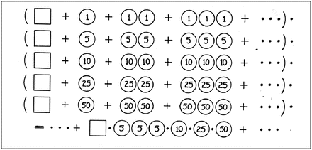
Pólya’s illustration of the change solution (courtesy Mathematical Association of America)
Full size image

We look at a related generating function for counting additive partitions in Example 3.4.6.
2.
Dissect a polygon with n sides into n − 2 triangles by n − 3 diagonals and compute D _n , the number of different dissections of this kind.

This is illustrated in Fig. 3.2 and leads to the fact that the generating function for $ {D}_3=1,{D}_4=2,{D}_5=5,{D}_6=14,{D}_7=42,\dots $
$$ \begin{array}{c}D(x)={\displaystyle \sum_{k=1}^{\infty }}{D}_k{x}^k\\ {}\end{array} $$
satisfies
$$ \begin{array}{c}D(x)=x\kern0.3em {\left[1+D(x)\right]}^2,\\ {}\end{array} $$
whose solution is therefore
$$ \begin{array}{c}D(x)=\frac{1-2x-\sqrt{1-4x}}{x}.\\ {}\end{array} $$
The Mathematica command
Fig. 3.2
The first few sets of dissections
Full size image

Series[((1 - 2 x) - Sqrt[1 - 4 x])/x, {x, 0, 10}]

returns
$$ \begin{array}{l}2x+4{x}^2+10{x}^3+28{x}^4+84{x}^5+264{x}^6+858{x}^7\hfill \\ {}\kern12pt +2860{x}^8+9724{x}^9+33592{x}^{10}+O\left({x}^{11}\right).\hfill \end{array} $$
with list of coefficients
$$ \{0,2,4,10,28,84,264,858,2860,9724,33592\} $$
and D _n+2 turns out to be the nth Catalan number $ \left(\genfrac{}{}{0ex}{}{2n}{n}\right)/ \left(n+1\right) $. This can be discovered using Sloane’s wonderful Online Encyclopedia of Integer Sequences as illustrated in Fig. 3.3. Note that we only used the first six non-zero terms and had four left to ‘confirm’ our experiment.
Fig. 3.3
Using https://oeis.org/ to identify the Catalan numbers
Full size image
3.
Compute T _n , the number of different (rooted) trees with n knots. ^{Footnote 9}

This is a significantly harder problem so we say less:

The ordinary generating function of the T _n becomes a remarkable result due to Cayley, namely
$$ T(x)={\displaystyle \sum_{k=1}^{\infty }}\kern0.3em {T}_k{x}^k=x\kern0.3em {\displaystyle \prod_{k=1}^{\infty }}\kern0.3em {\left(1-{x}^k\right)}^{-{T}_k}, $$
(3.3)
where remarkably the product and the sum share their coefficients. This can be used to produce a recursion for T _n in terms of $ {T}_1,{T}_2,\dots, {T}_{n-1} $, which starts: $ {T}_1=1,{T}_2=1,{T}_3=2,{T}_4=4,{T}_5=9,{T}_6=20,\dots $.

In each case, Pólya’s main message is that one can usefully draw pictures of the component elements—(a) in pennies, nickels dimes and quarters (plus loonies in Canada and half dollars in the USA), (b) in triangles and (c) in the simplest trees (with the fewest knots).

That said, I often find it easier to draw pictures from generating functions rather than go in the other direction. In any event, Pólya’s views on heuristic reasoning and his books on problem solving (Pólya, 1981, 1990) remain as engaging, if idiosyncratic, today as when first published.^{Footnote 10}

2.2.1 Proofs Without Words

In Fig. 3.4 we reproduce three classic proofs without words—though most such proofs benefit from a few words of commentary. In Fig. 3.5 we display three modern (dynamic geometry) proofs without words from http://cinderella.de/files/HTMLDemos/Main.html.^{Footnote 11}

Figure 3.4 shows from left to right the following three results:

1.
Pythagoras theorem;
2.
$ 1+3+5+\left(2n-1\right)={n}^2 $;
3.
$ 1/2+1/4+1/8+\cdots =1 $.

The Pythagorean proof is from the Zhou Bi Suan Jing which dates from the Zhou Dynasty (1046 BCE–256 BCE), and is one of the oldest recorded.

Figure 3.5 shows from left to right the following three results:

1.
Pythagoras theorem;
2.
$ \sqrt{2} $ is irrational as suggested by Tom Apostol^{Footnote 12};
3.
How to inscribe three tangent circles in a triangle.

Needless to say, the advantage of a modern construction—when there really is one—is largely lost on the printed page, which does not allow one to see the dynamics. We somewhat repair that damage in Fig. 3.6 by showing three illustrations of different configurations for fractals—zoom-invariant objects—built on circles of Apollonius.^{Footnote 13} In this case we perturbed slightly the configuration on the left to that in the middle and then the right, and see the different appearance of the fractals produced by the same rules.

3 Experimental Mathematics

The same ICMI study (2012), quoting (Borwein & Devlin, 2008, p. 1), says enough about the meaning of experimental mathematics for our current purposes:

Experimental mathematics is the use of a computer to run computations—sometimes no more than trial-and-error tests—to look for patterns, to identify particular numbers and sequences, to gather evidence in support of specific mathematical assertions that may themselves arise by computational means, including search.

Like contemporary chemists—and before them the alchemists of old—who mix various substances together in a crucible and heat them to a high temperature to see what happens, today’s experimental mathematicians put a hopefully potent mix of numbers, formulas, and algorithms into a computer in the hope that something of interest emerges.

3.1 Experimental Mathodology

I originally mistyped ‘mathodology’ intending ‘methodology’, but I liked the mistake and have kept it. We started (Borwein & Devlin, 2008) with Justice Potter Stewart’s famous 1964 comment on pornography: “I know it when I see it.”

A bit less informally, by experimental mathematics I intend, as discussed in Borwein and Bailey (2008) and elsewhere:

All of these uses play a central role in my daily research life. We will see all of these eight notions illustrated in the explicit examples of Sect. 3.3.2 and of Sect. 3.4.

3.2 When Science Becomes Technology

What tools we choose to use—and when—is a subtle and changeable issue.

Example 3.3.1 (When Science Becomes Technology).

We ‘unpack’ methods when we want to understand them or are learning them for the first time. Once we or our students have mastered a new tool we ‘repack’ it. For instance,

$$ {2}^{2^7}+1=340282366920938463463374607431768211457 $$

which factors as

$$ (59649589127497217)(5704689200685129054721). $$

If we are teaching or taking a course in factorization methods, we may well want to know ‘how’ this was done. In most contexts, we are happy to treat the computer as a reliable tool and to take the answer without further introspection.

In like fashion,

$$ t:=1.25992104989487316476721060728\dots =\sqrt[3]{2} $$

will be computed by most packages to the displayed precision. We can confirm this since

$$ {t}^3=2.00000000000000000000000000001\dots $$

If we wish to understand what the computer has done—probably by Newton’s method, we must go further, but if we only wish to use the answer that is irrelevant. The first is science or research, the second is technology. $ \diamondsuit $

The William Lowell Putnam competition taken each year by the strongest North American undergraduate students has conventionally had one easy question (out of 12) based on the current year.

Example 3.3.2 (A 1998 Putnam Examination Problem).

The problem was

Let N be the positive integer with 1998 decimal digits, all of them 1; that is, N = 1111…11. Find the thousandth digit after the decimal point of $ \sqrt{N} $.

This can be done by brute force

> evalf[10](sqrt(add(10^k,k=0..1997))/10^1000;

which is not what the posers had in mind. $ \diamondsuit $

Example 3.3.3 (A 1995 Putnam Examination Problem).

The problem requests

Evaluate:

$$ \sqrt[8]{2207-\frac{1}{2207-\frac{1}{2207-\dots }}} $$

(3.4)

Express your answer in the form $ \left(a+b\sqrt{c}\right)/ d $, where a, b, c, d are integers.

Proof.

If we call the repeated radical above α, the request is to solve for

$$ {\alpha}^8=2207-\frac{1}{2207-\frac{1}{2207-1/ {\alpha}^8}}, $$

and a solve request to a CAS will return

$$ {\left(\frac{2207}{2}+\frac{987\kern0.3em \sqrt{5}}{2}\right)}^{1/ 8}=\frac{3+\sqrt{5}}{2}. $$

(3.5)

We may determine the last reduction in many ways (1) via identify, (2) using the inverse symbolic calculator (ISC), (3) using a resolvent computation to find the quadratic polynomial satisfied by α as given by Eq. (3.5), or (4) by repeatedly computing the square root. Indeed identify will return the answer directly from (3.4) which already agrees with the limit to 20 places. □

With access to computation the problem becomes too straight-forward. $ \diamondsuit $

I next recall some continued fraction notation. Figure 3.7 shows the two most common ways of writing a simple or regular continued fraction—in this case for π. For any α > 0, this represents the process of going from

$$ \alpha \to {\alpha}^{\prime }:=\frac{1}{\alpha -\left\lfloor \alpha \right\rfloor } $$

and repeating the process, while recording the integer part $ \left\lfloor \alpha \right\rfloor $ each time. This is usually painful to do by hand but is easy for our computer.

Example 3.3.4 (Changing Representations).

Suppose I wish to examine the numbers

$$ \alpha :=0.697774657964007982006790592552 $$

and

$$ \beta :=0.92001690001910008622659579993. $$

As floating point numbers there is nothing to distinguish them; but the Maple instruction convert(alpha,confrac); returns the simple continued fraction for α in compact form (Borwein and Bailey, 2008)

$$ \alpha =\left[0,1,2,3,4,5,6,7,8,9,10,11,12,13,14,15,16,\dots \right] $$

while convert(beta,confrac); returns

$$ \beta =\left[0,1,11,1,1,94,6,2,9,2,1,5,1,6,7,3,4,24,1,8,1,2,1,2,1,\dots \right]. $$

So, in this new representation, the numbers no longer look similar. As described in Borwein and Bailey (2008), Borwein and Devlin (2008), and Bailey and Borwein (2011a), continued fractions with terms in arithmetic progression are well studied, and so there are several routes now open to discovering that $ \alpha ={I}_1(2)/ {I}_0(2) $ where for ν = 0, 1, 2, …

$$ {I}_{\nu }(2z)={z}^{\nu }{\displaystyle \sum_{k=0}^{\infty}\frac{{\left({z}^2\right)}^k}{k!\left(\nu +k\right)!}}. $$

For instance, on May 23, 2014, entering "continued fraction" "arithmetic progression" into Google returned 23,700 results of which the first http://mathworld.wolfram.com/ContinuedFractionConstant.html gives the reader all needed information, as will the use of the ISC. My purpose here was only to show the potential power of changing a representation. For example, the continued fraction of the irrational golden mean $ \frac{\sqrt{5}+1}{2}=1.6180339887499\dots $ is [1, 1, 1, …]. Figure 3.8 illustrates the golden mean, and also provides a proof without words that it is irrational as we discuss further in the next section.

It is a result of Lagrange that an irrational number is a quadratic if and only if it has a non-terminating but eventually repeating simple continued fraction. So quadratics are to continued fractions what rationals are to decimal arithmetic. This is part of their power. $ \diamondsuit $

As the following serious quotation makes clear, when a topic is science and when it is technology is both time and place dependent.

A wealthy (15th Century) German merchant, seeking to provide his son with a good business education, consulted a learned man as to which European institution offered the best training.“If you only want him to be able to cope with addition and subtraction,” the expert replied, “then any French or German university will do. But if you are intent on your son going on to multiplication and division – assuming that he has sufficient gifts – then you will have to send him to Italy.”^{Footnote 15}

3.2.1 Minimal Configurations

Both the central picture in Fig. 3.5 and the picture in Fig. 3.8 illustrate irrationality proofs. Traditionally, each would have been viewed as showing a reductio ad absurdum. Since the development of modern set theory and of modern discrete mathematics it is often neater to view them as deriving a contradiction from assuming some object is minimal.

For example, suppose that the (a + b) × a rectangle was the smallest integer rectangle representing the golden mean in Fig. 3.8, then the a × b rectangle cannot exist. Because of the geometric simplicity of this argument, it is thought that this may be the first number the Pythagoreans realized was irrational. Figure 3.5, by contrast, illustrates a reductio. If we continue, we will eventually get to an impossibly small triangle with integer sides. A clean picture for minimality is shown in Fig. 3.9.

Example 3.3.5 (Sylvester’s Theorem, Bailey & Borwein, 2011b).

The theorem conjectured by Sylvester in the late nineteenth century establishes that given a finite set of non-colinear points in the plane there is at least one ‘proper’ line through exactly two points. The first proof 40 years later was very complicated. Figure 3.10 shows a now-canonical minimality proof.

The objects used in this picture are pairs (L, p) where L is a line through at least two points of the set and p is the closest point in the set but not on the line. We consider the $ \left(\overline{L},\overline{p}\right) $ with $ \overline{p} $ closest to $ \overline{L} $. We assert that $ \overline{L} $ (the red horizontal line) has only two points of the set on it. If not two points lie on one side of the projection of $ \overline{p} $ on $ \overline{L} $. And now the black line L ₀ through $ \overline{p} $ and the farther point on L, and p ₀ the red point nearer to the projection constructs a configuration $ \left({L}_0,{p}_0\right) $ violating the minimality of $ \left(\overline{L},\overline{p}\right) $.

Subtle, ingenious and impossible to grasp without a picture! Here paper and coloured pencil are a fine tool. $ \diamondsuit $

3.3 Mathematical Discovery (or Invention)

Giaquinto’s attractive encapsulation: “In short, discovering a truth is coming to believe it in an independent, reliable, and rational way” Giaquinto (2007, p. 50) has the satisfactory consequence that a student can discover results whether known to the teacher or not. Nor is it necessary to demand that each dissertation be original (only that the results should be independently discovered).

Despite the conventional identification of mathematics with deductive reasoning, Kurt Gödel (1906–1978) in his 1951 Gibbs Lecture said: “If mathematics describes an objective world just like physics, there is no reason why inductive methods should not be applied in mathematics just the same as in physics”. He held this view until the end of his life despite—or perhaps because of—the epochal deductive achievement of his incompleteness results.

Also, one discovers that many great mathematicians from Archimedes and Galileo—who apparently said “All truths are easy to understand once they are discovered; the point is to discover them.”—to Gauss, Poincaré, and Carleson have emphasized how much it helps to “know” the answer. Two millennia ago Archimedes wrote to Eratosthenes^{Footnote 16} “For it is easier to supply the proof when we have previously acquired, by the method, some knowledge of the questions than it is to find it without any previous knowledge”. Think of the Method as an ur-precursor to today’s interactive geometry software—with the caveat that, for example, Cinderella actually does provide certificates for much Euclidean geometry.

As 2006 Abel Prize winner Lennart Carleson describes in his 1966 ICM speech on his positive resolution of Luzin’s 1913 conjecture (about the pointwise convergence of Fourier series for square-summable functions) after many years of seeking a counterexample he decided none could exist. The importance of this confidence is expressed as follows:

The most important aspect in solving a mathematical problem is the conviction of what is the true result. Then it took 2 or 3 years using the techniques that had been developed during the past 20 years or so.

3.4 Digital Assistance

By digital assistance I mean use of artefacts as:

1.
Modern Mathematical Computer Packages—symbolic, numeric, geometric or graphical. Symbolic packages include the commercial computer algebra packages Maple and Mathematica, and the open source SAGE. Primarily numeric packages start with the proprietary matlab and public counterparts Octave and NumPy, or the statistical package (R). The dynamic geometry offerings include Cinderella, Geometer’s Sketchpad, Cabri and the freeware GeoGebra.
2.
Specialized Packages or General Purpose Languages such as Fortran, C++, Python, CPLEX, PARI, SnapPea and MAGMA.
3.
Web Applications such as: Sloane’s Encyclopedia of Integer Sequences, the ISC,^{Footnote 17} Fractal Explorer, Jeff Weeks’ Topological Games, or Euclid in Java.^{Footnote 18}
4.
Web Databases including Google, MathSciNet, ArXiv, GitHub, Wikipedia, MathWorld, MacTutor, Amazon, Wolfram Alpha, the DLMF (Olver, Lozier, Boisvert, & Clark, 2012) (all formulas of which are accessible in MathML, as bitmaps, and in TE X) and many more that are not always so viewed.

All entail data-mining in various forms. Franklin (2005) argues Steinle’s “exploratory experimentation” facilitated by “widening technology”, as in pharmacology, astrophysics, medicine and biotechnology, is leading to a reassessment of what legitimates experiment; in that a “local model” is not now prerequisite. Sørenson (2010) cogently makes the case that experimental mathematics—as ‘defined’ above—is following similar tracks.

These aspects of exploratory experimentation and wide instrumentation originate from the philosophy of (natural) science and have not been much developed in the context of experimental mathematics. However, I claim that e.g., the importance of wide instrumentation for an exploratory approach to experiments that includes concept formation also pertain to mathematics.

In consequence, boundaries between mathematics and the natural sciences and between inductive and deductive reasoning are blurred and getting more so. (See also Avigad, 2008.) I leave unanswered the philosophically vexing if mathematically minor question as to whether genuine mathematical experiments (as discussed in Borwein & Bailey, 2008) exist even if one embraces a fully idealist notion of mathematical existence. They sure feel like they do.

3.5 The Twentieth Century’s Top Ten Algorithms

The modern computer itself, being a digital repurposable tool, is quite different from most of its analogue precursors. They could only do one or two things. The digital computer, of course, greatly stimulated both the appreciation of and need for algorithms and for algorithmic analysis.^{Footnote 19} These are what allows the repurposing. This makes it reasonable to view substantial mathematical algorithms as tools in their own right.

At the beginning of this century, Sullivan and Dongarra could write “Great algorithms are the poetry of computation”, when they compiled a list of the ten algorithms having “the greatest influence on the development and practice of science and engineering in the twentieth century”.^{Footnote 20} Chronologically ordered, they are:

#1.
1946: The Metropolis Algorithm for Monte Carlo. Through the use of random processes, this algorithm offers an efficient way to stumble toward answers to problems that are too complicated to solve exactly.
#2.
1947: Simplex Method for Linear Programming. An elegant solution to a common problem in planning and decision-making.
#3.
1950: Krylov Subspace Iteration Method. A technique for rapidly solving the linear equations that abound in scientific computation.
#4.
1951: The Decompositional Approach to Matrix Computations. A suite of techniques for numerical linear algebra.
#5.
1957: The Fortran Optimizing Compiler. Turns high-level code into efficient computer-readable code.
#6.
1959: QR Algorithm for Computing Eigenvalues. Another crucial matrix operation made swift and practical.
#7.
1962: Quicksort Algorithms for Sorting. For the efficient handling of large databases.
#8.
1965: Fast Fourier Transform (FFT). Perhaps the most ubiquitous algorithm in use today, it breaks down waveforms (like sound) into periodic components.
#9.
1977: Integer Relation Detection. A fast method for spotting simple equations satisfied by collections of seemingly unrelated numbers.
#10.
1987: Fast Multipole Method. A breakthrough in dealing with the complexity of n-body calculations, applied in problems ranging from celestial mechanics to protein folding.

I observe that eight of these ten winners appeared in the first two decades of serious computing, and that Newton’s method was apparently ruled ineligible for consideration.^{Footnote 21} Most of the ten are multiply embedded in every major mathematical computing package. The last one is the only one that occurs infrequently in my own work.

Just as layers of software, hardware and middleware have stabilized, so have their roles in scientific and especially mathematical computing. When I first taught the simplex method more than 30 years ago, the texts concentrated on ‘Y2K’-like tricks for limiting storage demands.^{Footnote 22} Now serious users and researchers will often happily run large-scale problems in Matlab and other broad spectrum packages, or rely on CPLEX or, say, NAG library routines embedded in Maple.

While such out-sourcing or commoditization of scientific computation and numerical analysis is not without its drawbacks, I think the analogy with automobile driving in 1905 and 2005 is apt. We are now in possession of mature—not to be confused with ‘error-free’—technologies. We can be fairly comfortable that Mathematica is sensibly handling round-off or cancellation error, using reasonable termination criteria and the like. Below the hood, Maple is optimizing polynomial computations using tools like Horner’s rule, running multiple algorithms when there is no clear best choice, and switching to reduced complexity (Karatsuba or FFT-based) multiplication when accuracy so demands. Though, it would be nice if all vendors allowed as much peering under the bonnet as Maple does.

3.6 Secure Knowledge Without Proof

Given real floating point numbers

$$ \beta, {\alpha}_1,{\alpha}_2,\dots, {\alpha}_n, $$

Helaman Ferguson’s integer relation method—see #9 of Sect. 3.3.5 above—called unhelpfully PSLQ, finds a nontrivial linear relation of the form

$$ {a}_0\beta +{a}_1{\alpha}_1+{a}_2{\alpha}_2+\cdots +{a}_n{\alpha}_n=0, $$

(3.6)

where a _i are integers—if one exists and provides an exclusion bound otherwise. This method is very robust. Given adequate precision of computation (Borwein and Bailey, 2008) it very rarely returns spurious relations.

If a ₀ ≠ 0, then (3.6) assures β is in the rational vector space generated by

$$ \left\{{\alpha}_1,,,{\alpha}_2,,,\dots,,, {\alpha}_n\right\}. $$

Moreover, as a most useful special case, if $ \beta :=1,{\alpha}_i:={\alpha}^i $, then α is algebraic of degree n (see Example 3.4.9).

Quite impressively here is an unproven 2010 integer relation discovery by Cullen:

$$ \frac{2^{11}}{\pi^4}\overset{?}{=}{\displaystyle \sum_{n=0}^{\infty }}\frac{{\left(\frac{1}{4}\right)}_n{\left(\frac{1}{2}\right)}_n^7{\left(\frac{3}{4}\right)}_n}{(1)_n^9}\left(21+466n+4340{n}^2+20632{n}^3+43680{n}^4\right){\left(\frac{1}{2}\right)}^{12n}. $$

(3.7)

We have no idea why it is true but you can check it to almost any precision you wish. In Example 3.4.10 we shall explore such discoveries.

3.7 Is ‘Free’ Software Better?

I conclude this section by commenting on open-source versus commercial software. While free is very nice, there is no assurance that most open source projects such as GeoGebra (based on Cabri and now very popular in schools as replacement for Sketchpad) will be preserved when the founders and typically small core group of developers lose interest or worse. This is still an issue with large-scale commercial products but a much smaller one.

I personally prefer Maple to Mathematica as most of the source code is accessible, while Mathematica is entirely sealed. This is more of an issue for researchers than for educators or less intense users. Similarly, Cinderella is very robust, unlike GeoGebra, and mathematically sophisticated—using Riemann surfaces to ensure that complicated constructions do not crash. That said, it is the product of two talented and committed mathematicians but only two, and it is only slightly commercial. In general, software vendors and open source producers do not provide the teacher support that has been built into the textbook market.

4 A Dozen or So Accessible Examples

Modern graphics tools change traditional approaches to many problems. We used to teach calculus techniques to allow graphing of even reasonably simple functions. Now one should graph to be guided in doing calculus.

Example 3.4.1 (Graphing to Do Calculus).

Consider a request in a calculus text to compare the function given by $ f(y):={y}^2 \log y $ (red) to each of the functions given by $ g(y):=y-{y}^2 $ and $ h(y):={y}^2-{y}^4 $ for $ 0\leqslant y\leqslant 1 $; and to prove any inequality that holds on the whole unit interval.

The graphs of f, g are shown in the left of the picture in Fig. 3.11, and the graphs of f, h to the right. In any plotting tool we immediately see that f and g cross but that $ h\geqslant f $ appears to hold on [0, 1]. Only in a neighbourhood of 1 is there any possible doubt. Zooming in—as is possible in most graphing tools—or re-plotting on a smaller interval around 1 will persuade you that f(y) > h(y) for 0 < y < 1. This is equivalent to $ k(x):= \log (x)-1+1/ x>0 $ and so that is what you try to prove. Now it is immediate that k′(x) < 0 on the interval and so k strictly decreases to k(1) = 0 and we are done.□

Likewise, computer algebra systems (CAS) now make it possible to find patterns which we prove ex post facto by induction. Before CAS many of these inductive statements might have been inaccessible.

Example 3.4.2 (Induction and Computer Algebra).

We all know how to show

$$ {\displaystyle \sum_{k=1}^N}k=\frac{n\left(n+1\right)}{2} $$

with or without induction. But what about

$$ {\displaystyle \sum_{k=1}^N}{k}^5=? $$

Consider the following three lines of Maple code.

> S:=(n,N)->sum(k^n,k=1..N):

> S5:=unapply(factor(simplify(S(5,N))),N);

> simplify(S5(N)-S5(N-1));

The first line defines the sum $ {\displaystyle {\sum}_{k=1}^N}{k}^n $. The second finds this sum for n = 5 and makes it into a function of N. We obtain:

$$ {\displaystyle \sum_{k=1}^N}{k}^5=\frac{1}{12}\kern0.3em {N}^2\left(2\kern0.3em {N}^2+2\kern0.3em N-1\right){\left(N+1\right)}^2. $$

(3.8)

The third line proves this by induction—on checking that S5(1) = 1. The proof can of course be done by hand. Jakob Bernoulli (1655–1705) invented his Bernoulli numbers ^{Footnote 23} and associated polynomials in part to evaluate such sums. Indeed, using the same code with N = 10 we arrive at a proof that

$$ {\displaystyle {\sum}_{k=1}^N}{k}^{10}=\frac{N\left(2\kern0.3em N+1\right)\left(N+1\right)\left({N}^2+N-1\right)\left(3\kern0.3em {N}^6+9\kern0.3em {N}^5+2\kern0.3em {N}^4-11\kern0.3em {N}^3+3\kern0.3em {N}^2+10\kern0.3em N-5\right)}{66} $$

and so that

$$ {\displaystyle \sum_{k=1}^{100}}{k}^{10}=959924\underline{142434241}924250, $$

and

$$ {\displaystyle \sum_{k=1}^{1000}}{k}^{10}=9140992424\underline{1424243424241}924242500. $$

This later computation by Bernoulli is accounted as the first case of real computational number theory. Likewise

$$ {\displaystyle \sum_{k=1}^{10000}}{k}^{10}=90959099242424\underline{14242424342424241}924242425000. $$

We finish with interior palindromes in each of the three sums centered at the ‘3’ and leave its explanation and other apparent patterns to the reader. Of course, unlike Bernoulli, we could simply have added the three sums without finding the closed form but then we would know much less.□

Large matrices often have structure that pictures will reveal but which numeric data may obscure.

Example 3.4.3 (Visualizing Matrices).

The picture in Fig. 3.12 shows a 25 × 25 Hilbert matrix on the left and on the right a matrix required to have 50 % sparsity and non-zero entries random in [0, 1].

The 4 × 4 Hilbert matrix in Maple is generated by with(LinearAlgebra); HilbertMatrix(4); which code produces

$$ \left[\begin{array}{cccc}1& 1/ 2& 1/ 3& 1/ 4\\ {}1/ 2& 1/ 3& 1/ 4& 1/ 5\\ {}1/ 3& 1/ 4& 1/ 5& 1/ 6\\ {}1/ 4& 1/ 5& 1/ 6& 1/ 7\end{array}\right] $$

from which the general definition should be apparent. Hilbert matrices are notoriously unstable numerically. The picture on the left of Fig. 3.13 shows the inverse of the 20 × 20 Hilbert matrix when computed symbolically and so exactly. The picture in the middle shows the enormous numerical errors introduces if one uses 10 digit precision, and the right shows that even if one uses 20 digits, the errors are less frequent but even larger.

Representative Maple code for drawing the symbolic inverse is:

> with(plots):

> matrixplot(MatrixInverse(HilbertMatrix(20)),

heights = histogram, axes = frame, gap = .2500000000,

color = proc (x, y) options operator, arrow; sin(y*x) end proc);}

It is very good fun to play with pictures of very large matrices constructed to have complicated block structure. Consider the sequence of 2n × 2n matrices Q(n), with entries only 0, 1, 2, 4 which start

$$ \left[\begin{array}{cc}2& 1\\ {}0& 1\end{array}\right].\kern2em \left[\begin{array}{cccc}2& 2& 1& 0\\ {}0& 2& 2& 1\\ {}0& 0& 1& 1\\ {}0& 0& 0& 1\end{array}\right],\kern2em \left[\begin{array}{cccccc}2& 2& 2& 1& 0& 0\\ {}0& 2& 4& 2& 1& 0\\ {}0& 0& 2& 2& 2& 1\\ {}0& 0& 0& 1& 1& 1\\ {}0& 0& 0& 0& 1& 2\\ {}0& 0& 0& 0& 0& 1\end{array}\right] $$

(3.9)

We cannot possibly present Q(100) as a symbolic or numerical matrix but Fig. 3.14 visually shows everything both about the matrix and its inverse.□

Let us continue with a different exploration of matrices.

Example 3.4.4 (Abstract Becomes Concrete).

Define, for n > 1 the n × n matrices A(n), B(n), C(n), M(n) by

$$ \begin{array}{l}{A}_{kj}={(-1)}^{k+1}\left(\genfrac{}{}{0ex}{}{2n-j}{2n-k}\right),\kern1em {B}_{kj}={(-1)}^{k+1}\left(\genfrac{}{}{0ex}{}{2n-j}{k-1}\right),\hfill \\ {}{C}_{kj}={(-1)}^{k+1}\left(\genfrac{}{}{0ex}{}{j-1}{k-1}\right)\hfill \end{array} $$

(for k, j = 1, …, n) and set $ M:=A+B-C $. For instance,

$$ M(7)=\left[\begin{array}{ccccccc}1& 0& 0& 0& 0& 0& 0\\ {}26& -12& 9& -7& 5& -3& 1\\ {}156& -78& 55& -42& 30& -18& 6\\ {}572& -286& 176& -120& 80& -46& 15\\ {}1430& -715& 385& -220& 126& -65& 20\\ {}2574& -1287& 627& -297& 135& -56& 15\\ {}3432& -1716& 792& -330& 120& -36& 7\end{array}\right]. $$

In my research (Borwein, Bailey, & Girgensohn, 2005, §3.3), I needed to show M(n) was invertible. After staring at numerical examples without much profit, I decided to ask Maple for the minimal polynomial of M(10) using

> MP:=LinearAlgebra[MinimalPolynomial]: MP(evalm(M(10)),t);

and was surprised to get $ {t}^2+t-2 $. (One way to write B in Maple is

> B:=n->matrix(n,n,(i,j)->(-1)^(j+1)*binomial(2*n-j,i-1));

and there are many other formats.) I got the same answer for M(30) and so I knew $ M{(n)}^2+M(n)=2I $ for all n > 1 or equivalently that

$$ {M}^{-1}=\frac{M+I}{2}. $$

But why? I decided to explore A, B, C with the same tool and discovered that A and C satisfied t ² = 1 and B satisfied t ³ = 1. This led me to realize that A, B, C generated the symmetric group on three elements and so to a computer discovered proof that M was as claimed.

As an illustration of the robustness of such discoveries, if we change the $ i=1,j=10 $ entry in M(10) to ε ≠ 0 from 0, we find the minimal polynomial is far from as simple: ${t^4} + 2\;{t^3} - 3\;{t^2} - 4\;t + 4 - \left( {252\;{t^2} + 252\;t - 504} \right),$ which also shows the discontinuity at ε = 0. Similarly, for the 5 × 5 Hilbert matrix we get

$$ \begin{array}{ll}\hfill & -\frac{1}{266716800000}+\frac{61501\kern0.3em t}{53343360000}-\frac{852401\kern0.3em {t}^2}{222264000}+\frac{735781\kern0.3em {t}^3}{2116800}-\frac{563\kern0.3em {t}^4}{315}+{t}^5=0.\end{array} $$

The constant term is of course giving minus the determinant. When I was a student characteristic and minimal polynomials seemed to be entirely abstract and matrix decompositions were in their infancy. Now they are technology. $ \diamondsuit $

Example 3.4.5 (Hardy’s Taxi-Cab).

Hardy when visiting Ramanujan in hospital in 1917 remarked that his taxi’s number, 1729, was very dull. Ramanujan famously replied that it was very interesting being the smallest number expressible as a sum of two cubes in two distinct ways (not counting sign or order):

$$ 1729=1{2}^3+{1}^3=1{0}^3+{9}^3. $$

Let us ask “what is the second such number? As in Sect. 3.2.2, we can look at a generating function—this time for cubes. The coefficients of C ²(q) will be 0 when n is not the sum of two cubes, 1 when n = 2m ³, 2 when $ n={m}^3+{k}^3 $ for k ≠ m. If there are two distinct representations, the coefficient will be 4. The Maple fragment

> C:=convert((add(q^(n^3),n=1..20)^2),polynom):C-(C mod 4):

outputs $ 4\kern0.3em {q}^{4104}+4\kern0.3em {q}^{1729} $ which both proves Ramanujan’s assertion and finds that the second example is $ 4104=1{5}^3+{9}^3={2}^3+1{6}^3 $. If we change 20–25 in our code, we uncover the third such number. Alternatively entering just the first two into the OIES produces sequence A001235 consisting of the ‘taxi-cab numbers’: 1729, 4104, 13832, 20683, 32832, 39312, 40033, 46683, 64232, 65728, 110656, 110808, … $ \diamondsuit $

Example 3.4.6 (Euler’s Pentagonal Number Theorem).

The number of additive partitions of n, p(n), is generated by

$$ P(q)=1+{\displaystyle \sum_{n\geqslant 1}}p(n){q}^n={\displaystyle \prod_{n\geqslant 1}}{\left(1-{q}^n\right)}^{-1}. $$

(3.10)

Thus p(5) = 7 since

$$ \begin{array}{l}5=4+1=3+2=3+1+1=2+2+1\hfill \\ {}\kern1.45em =2+1+1+1=1+1+1+1+1,\hfill \end{array} $$

as we ignore “0” and permutations. Additive partitions are mathematically less tractable than multiplicative ones as there is no analogue of unique prime factorization nor the corresponding structure.

Partitions provide a wonderful example of why Keith Devlin calls mathematics “the science of patterns”. They do sometimes enter the school curriculum through the back-door in the guise of Cuisenaire rods (or réglets), as illustrated by a staircase in Fig. 3.15.

Formula (3.10) is easily seen by expanding $ {\left(1-{q}^n\right)}^{-1} $ and comparing coefficients. A modern computational temperament leads to:

Question: How hard is p(n) to compute—in 1900 (for MacMahon the “father of combinatorial analysis”) or in 2015 (for Maple or Mathematica)?

Answer: The famous computation by Percy MacMahon of p(200) = 3972999029388 at the beginning of the twentieth century, done symbolically and entirely naively from (3.10) in Maple on a laptop, took 20 min in 1991 but only 0.17 s in 2010, while the many times more demanding computation

$$ p(2000)=4720819175619413888601432406799959512200344166 $$

took just 2 min in 2009 and 40.7 s in 2014.^{Footnote 24} Moreover, in December 2008, the late Richard Crandall was able to calculate p(10⁹) in 3 s on his laptop, using the Hardy-Ramanujan-Rademacher ‘finite’ series for p(n) along with FFT methods. Using these techniques, Crandall was also able to calculate the probable primes p (1000046356) and p(1000007396), each of which has roughly 35, 000 decimal digits.^{Footnote 25}

Such results make one wonder when easy access to computation discourages innovation: Would Hardy and Ramanujan have still discovered their marvelous formula for p(n) if they had powerful computers at hand? The Maple code

N:=500; coeff(series(1/product(1-q^n,n=1..N+1),q,N+1),q,N);

Twenty-five years ago computing P(q) in Maple was very slow, while taking the series for the reciprocal of the series for

$$ Q(q)={\displaystyle \prod_{n\geqslant 1}}\left(1-{q}^n\right) $$

was quite manageable!

Why? Clearly the series for Q must have special properties. Indeed it is lacunary:

$$ Q(q)=1-q-{q}^2+{q}^5+{q}^7-{q}^{12}-{q}^{15}+{q}^{22}+{q}^{26}-{q}^{35}-{q}^{40}+{q}^{51}+{q}^{57}-{q}^{70}-{q}^{77}+{q}^{92}+O\left({q}^{100}\right). $$

(3.11)

This lacunarity is now recognized automatically by Maple, so the platform works much better, but we are much less likely to discover Euler’s gem:

$$ {\displaystyle \prod_{n=1}^{\infty }}\left(1-{q}^n\right)={\displaystyle \sum_{n=-\infty}^{\infty }}{\left(-1\right)}^n{q}^{n\left(3n+1\right)/ 2}. $$

If we do not immediately recognize the pentagonal numbers, $ \left(3\left(n+1\right)n/ 2\right) $, then Sloane’s online Encyclopedia of Integer Sequences ^{Footnote 26} again comes to the rescue with abundant references to boot.

This sort of mathematical computation is still in its reasonably early days but the impact is palpable.□

Example 3.4.7 (Ramanujan’s Partition Congruences).

Ramanujan had access to the first 200 values of p(n) thanks to MacMahon’s lengthy work which the following Maple snippet reconstructs near instantly:

> N:=200:L200:=

sort([coeffs(convert(series(1/product(1-q^n,n=1..N+1),q,N+1),polynom))]);

The list starts 1, 1, 2, 3, 5, 7, 11, 15, 22, 30, 42, 56, 77, 101, 135, 176, 231, 297, 385, 490, 627… with p(0): = 1, and Ramanujan noted various modular patterns. Namely p(5n + 4) is divisible by 5, and p(7n + 5) is divisible by 7. This is hard to see from a list but a little software can help. The snippet below reshapes the beginning of a list of n × m or more entries into an n × m matrix:

> reshape:=proc (L, n, m) local k;

linalg[matrix](n, m, [seq(L[k], k = 1 .. m*n)])

end proc

For instance, > reshape(L200 mod 5, 8,20) produces the first 160 entries of the list with 20 columns in each of 8 rows as

$$ \left[\begin{array}{cccccccccccccccccccc}1& 1& 2& 3& 0& 2& 1& 0& 2& 0& 2& 1& 2& 1& 0& 1& 1& 2& 0& 0\\ {}2& 2& 2& 0& 0& 3& 1& 0& 3& 0& 4& 2& 4& 3& 0& 3& 2& 2& 0& 0\\ {}3& 3& 4& 1& 0& 4& 3& 4& 3& 0& 1& 3& 4& 1& 0& 1& 3& 4& 0& 0\\ {}2& 0& 1& 4& 0& 3& 0& 4& 0& 0& 3& 0& 3& 4& 0& 4& 1& 3& 4& 0\\ {}1& 2& 0& 4& 0& 2& 2& 3& 4& 0& 3& 4& 2& 2& 0& 4& 4& 0& 1& 0\\ {}2& 1& 4& 0& 0& 4& 1& 4& 4& 0& 1& 3& 1& 3& 0& 1& 3& 1& 3& 0\\ {}0& 1& 2& 1& 0& 2& 2& 0& 0& 0& 0& 4& 4& 2& 0& 1& 0& 1& 1& 0\\ {}0& 3& 0& 2& 0& 4& 4& 3& 2& 0& 3& 2& 1& 4& 0& 2& 4& 4& 2& 0\end{array}\right]. $$

We now see only zeroes in the columns congruent to 4 modulo 5 and discover the first congruence 5∣p(5n + 4). Similarly, > reshape(L200 mod 7, 8,21) reveals

$$ \left[\begin{array}{ccccccccccccccccccccc}1& 1& 2& 3& 5& 0& 4& 1& 1& 2& 0& 0& 0& 3& 2& 1& 0& 3& 0& 0& 4\\ {}1& 1& 2& 0& 5& 0& 0& 1& 1& 4& 3& 5& 0& 4& 1& 1& 0& 3& 0& 0& 0\\ {}2& 2& 2& 3& 5& 0& 0& 2& 1& 4& 0& 0& 0& 0& 3& 2& 2& 3& 5& 0& 4\\ {}2& 2& 2& 3& 5& 0& 4& 3& 2& 4& 6& 5& 0& 0& 2& 2& 4& 3& 5& 0& 0\\ {}3& 3& 6& 6& 3& 0& 1& 3& 3& 4& 3& 5& 0& 0& 4& 3& 4& 6& 5& 0& 1\\ {}5& 3& 6& 6& 3& 0& 0& 5& 4& 6& 6& 3& 0& 4& 5& 4& 6& 6& 5& 0& 0\\ {}6& 5& 1& 2& 3& 0& 1& 5& 5& 1& 6& 3& 0& 4& 0& 5& 1& 5& 1& 0& 1\\ {}0& 6& 3& 2& 1& 0& 4& 1& 6& 3& 5& 1& 0& 1& 1& 6& 3& 2& 1& 0& 1\end{array}\right] $$

and ‘discovers’ the second congruence 5∣p(7n + 5) for all $ n\geqslant 0 $. The third congruence 6∣p(11n + 6) for all $ n\geqslant 0 $ can be discovered by appropriate reshaping—and if wished confirmed by taking more terms. These partition congruences are discussed and the first two proved in Borwein and Borwein (1987, §3.5). $ \diamondsuit $

Maple has since version 9.5 had a function called ‘identify’. It takes many tools such as PSLQ (Sect. 3.3.6) and attempts to predict an answer for a floating point number. A related ISC is on-line at http://isc.carma.newcastle.edu.au/. This lets you enter a real number or a Maple expression and ask the computer “What is that number?”

Another excellent example of how packages are changing mathematics is the Lambert W function (Borwein et al., 2005), whose remarkable properties and development are very nicely described in a fairly recent article by Hayes (2005), Why W? Informally, W(x) solves

$$ x=W(x){e}^{W(x)}. $$

As a real function, its domain is $ \left(-1/ e,\infty \right) $. We draw W and the quite similar $ \log $ function on the left of Fig. 3.16. Its use can be traced back to Lambert (1728–1727), and W as a notation was used by Pólya and Szegö in 1925. However, this very useful non-elementary function only came into general currency after it was named and then implemented in both Maple and Mathematica. It is hard to use or popularize an un-named function. Now most CAS know the expansion

$$ W(z)={\displaystyle \sum_{k=1}^{\infty }}\frac{{\left(-k\right)}^{k-1}}{k!}{z}^k $$

with radius of convergence 1/e.

Example 3.4.8 (Solving Equations with W).

We first look at $ {x}^y={y}^x $.

(a)
Let us fix x > 0 and try to solve
$$ {x}^y={y}^x\kern1.5em \mathrm{f}\mathrm{o}\mathrm{r}\ y>0. $$
(3.12)
Of course, we seek a non-trivial solution with x ≠ y such as $ x=2,y=4 $. The Maple solve command returns
$$ y(x)=\left(\frac{-x}{ \log x}\right)W\left(\frac{- \log x}{x}\right). $$
(3.13)
This may confuse initially more than help. If we take logarithms in (3.12) and rearrange, we are trying to solve
$$ \frac{ \log y}{y}=z:=\frac{ \log x}{x} $$
(3.14)
for y > 0.

The right of Fig. 3.16 shows that the function $ \left( \log x\right)/ x $ is positive only on $ 1<x<\infty $ and then and only then has two solutions—except for x = e where the maximum of 1∕e occurs—and now in Maple solve(log(x)/x=z,x) returns $ -W\left(- \log\ z\right)/ z $. This solution is shown on the left in Fig. 3.17 where z implicitly must satisfy 0 < z < 1∕e. This yields (3.13), shown in the center of Fig. 3.17, where we know now that x > 1 is requisite. For instance, $ {y}_3:=-3W(-( \log \kern0.15em 3)/ 3)/ \log \kern0.15em 3=2.478052685\dots \ne 3 $ solves $ {3}^{y_3}={\left({y}_3\right)}^3. $
Fig. 3.17
(L) Solution to (3.13). (M) Solution to (3.12). (R) Quadratic Taylor approximation around e
Full size image

Now, we may not know W but our computer certainly now does. For instance, identify(0.56714329040978) returns W(1) and the Taylor series for y(x) around e starts
$$ \begin{array}{l}y(x)=\mathrm{e}-\mathrm{sign}\kern0.15em \left(x-\mathrm{e}\right)\left(x-\mathrm{e}\right)+\frac{5\kern0.3em {\mathrm{e}}^{-1}\left(\mathrm{sign}\left(x-\mathrm{e}\right)+1\right)}{6}{\left(x-\mathrm{e}\right)}^2\\ {}\kern2.65em +O\left({\left(x-\mathrm{e}\right)}^3\right)\hfill \end{array} $$
(3.15)
as shown on the right of Fig. 3.17. For x > e, $ y(x)=1/ (3\mathrm{e})\left(11\kern0.3em {\mathrm{e}}^2-13\kern0.3em x\mathrm{e}+5\kern0.3em {x}^2\right) $ while for x < e we get the trivial solution x.
(b)
A parametric form of the solution is $ x={r}^{1/ \left(r-1\right)},y=rx={r}^{r/ \left(r-1\right)} $, for r > 1. Equivalently with $ r=1+1/ s $, where s > 0, we have $ x={(1+1/ s)}^s,y={(1+1/ s)}^{s+1} $. This is shown in Fig. 3.18.
Fig. 3.18
Parametric solutions of (3.12) separated by y = e
Full size image
(c)
Repeated exponentiation. How many distinct meanings may be assigned to product towers for the n-fold exponentiation
$$ {x}^{\ast_n^x}={x}^{x^{x^{x{\cdots}^x}}}? $$

Recursions like x ₁ = t > 0 and $ {x}_n={t}^{x_{n-1}} $ for n > 0 have been subjected to considerable scrutiny. We can check that the solution to t ^x = x is $ t\mapsto -W\left(- \log \kern0.2em t\right)/ \log \kern0.2em t $ which solution exists for $ t\in \left[{e}^{-e},{e}^{1/ e}\right] $. $ \diamondsuit $

Example 3.4.9 (Finding Algebraic Numbers).

Both Maple and Mathematica have algorithms that can predict if a number is algebraic and even find its minimal polynomial. We described this a little further in Sect. 3.3.6. For instance, using identify—with no tuning of parameters—as with

> Digits:=20:a:=evalf(7^(1/2)+3^(1/2));identify(a);

returns

$$ \sqrt{7}+\sqrt{3} $$

but

> Digits:=20:a:=evalf(2^(1/3)+3^(1/2));identify(a);

returns

$$ 2.9919718574637504583 $$

meaning Maple could not identify the surd from 20 digits. The ISC at http://isc.carma.newcastle.edu.au/advancedCalc runs tuned algorithms and will identify the constant as shown in Fig. 3.19.

However:

> Digits:=30:a:=evalf(2^{1/3}+3^{1/2});identify(a);

returns

$$ Root\kern.5em Of\left({}_{-}{Z}^6-{9}_{-}{Z}^4-{4}_{-}{Z}^3+{27}_{-}{Z}^2-{36}_{-}Z-23, index=1\right) $$

which allows us to recover $ {2}^{1/ 3}+{3}^{1/ 2} $. For example, we can factor in $ \mathrm{Q}\left(\sqrt{3}\right) $ using the command:

> factor(_Z^6-9*_Z^4-4*_Z^3+27*_Z^2-36*_Z-23,sqrt(3));

which yields

$$ -\left(3\kern0.3em {\sqrt{3}}_{-}{Z}^2+{}_{-}{Z}^3+3\kern0.3em \sqrt{3}+{9}_{-}Z-2\right)\left(3\kern0.3em {\sqrt{3}}_{-}{Z}^2-{}_{-}{Z}^3+3\kern0.3em \sqrt{3}-{9}_{-}Z+2\right). $$

The quadratic formula now applies to determine that the only real roots of the sextic polynomial are $ {2}^{1/ 3}\pm \sqrt{3} $.□

We can do more exciting things of this kind.

Example 3.4.10 (What is that Number?).

Let us illustrate it for the integral

$$ \mathcal{R}(a):=\mathcal{R}\left(a,a\right)=2\underset{0}{\overset{1}{\int }}\kern0.3em \frac{t^{1/ a}}{1+{t}^2}\kern0.3em \mathrm{d}t $$

(3.16)

whose origins are described in Sect. 3.5. We plot R(a) in Fig. 3.20. (We used the hypergeometric form given below. Maple will find this form if you input (3.16).) Note that the graph is consistent with the fact that $ \mathcal{R} $ increases to the blue asymptote $ \mathcal{R}\left(\infty \right)=\frac{\pi }{2}. $ You may be able to evaluate some other values by hand.

Most CAS will answer that the values of $ \mathcal{R}\left(1/ m\right) $, for $ 1\leqslant m\leqslant 6 $, are

$$ \log 2,\kern1em 2-\frac{\pi }{2},\kern.5em 1- \log 2,\kern1em -\frac{4}{3}+\frac{\pi }{2},\kern.5em -\frac{1}{2}+ \log 2,\kern1em \frac{26}{15}-\frac{\pi }{2}. $$

We then check that $ \mathcal{R}\left(1/ 7\right)=\frac{5}{6}- \log 2 $ and $ \mathcal{R}\left(1/ 8\right)=-\frac{152}{105}+\frac{\pi }{2} $. From this it should be plausible that

$$ \begin{array}{c}{(-1)}^n\mathcal{R}\left(\frac{1}{2n+1}\right)= \log 2+{a}_n\\ {}{(-1)}^n\mathcal{R}\left(\frac{1}{2n}\right)=\frac{\pi }{2}+{b}_n\\ {}\end{array} $$

for rational numbers $ {a}_n,{b}_n $. As experimental confirmation of this conjecture we can check that

$$ \mathcal{R}\left(\frac{1}{21}\right)=-\frac{1627}{2520}+ \log 2,\kern1em \mathcal{R}\left(\frac{1}{20}\right)=-\frac{22128676}{14549535}+\frac{\pi }{2}. $$

If we ask the computer for $ \mathcal{R}(2) $, we get a complicated (ostensibly complex) expression that simplifies to $ \frac{\sqrt{2}}{4}\left(2\kern0.3em \pi + \log \left(17-12\kern0.3em \sqrt{2}\right)\right). $ If we try PSLQ for $ a:=2,2/ 3,2/ 5,\dots $ we discover that each such sum evaluates in terms of three basis vectors:

$$ 1,\sqrt{2}\pi \kern1em \mathrm{and}\kern1em \sqrt{2} \log \left(1+\sqrt{2}\right). $$

For instance,

$$ \mathcal{R}\left(\frac{11}{2}\right)=\frac{164}{45}-\frac{\pi }{\sqrt{2}}-\sqrt{2}\kern0.3em \log \left(1+\sqrt{2}\right). $$

If, however, we leave out the constant term ‘1’, we find

$$ \mathcal{R}(2)=\frac{\pi }{\sqrt{2}}-\sqrt{2}\kern0.3em \log \left(1+\sqrt{2}\right) $$

but have no such luck as we need that pesky constant term.

Actually, Borwein, Crandall, and Fee (2004) give a closed form for every instance of $ \mathcal{R}\left(\frac{p}{q}\right) $ with p, q positive integers.□

We turn to another example where the CAS provides a proof that we would not have been likely to arrive at without the current tools.

Example 3.4.11 (π Is Not 22∕7).

Even Maple or Mathematica ‘knows’ this since

$$ \begin{array}{c}0<{\int}_0^1\frac{(1-x)^4{x}^4}{1+{x}^2}\kern0.3em \mathrm{d}\mathrm{x}\kern2.77695pt =\kern2.77695pt \frac{22}{7}-\pi, \end{array} $$

(3.17)

though it would be prudent to ask ‘why’ it can perform the integral and ‘whether’ to trust it?

1.
Assuming we trust our software, the integrand is strictly positive on (0, 1), see Fig. 3.21, and so the answer in (3.17) is an area which is necessarily strictly positive, despite millennia of claims that π is 22∕7.
Fig. 3.21
The integrand in (3.17)
Full size image
2.
Quite accidentally, 22∕7 is one of the early continued fraction approximation to π—and is why it is a pretty reasonable approximation to π. These commence:
$$ 3,\frac{22}{7},\frac{333}{106},\frac{355}{113},\dots $$
but no one has found a way to replicate (3.17) for these other fractions. Some coincidences are just that—happenstance. Similarly, there is no good reason why $ {e}^{\pi }-\pi =\underline{19.9990999}7918947576\dots $, but it is most impressive on a low precision calculator.
3.
We turn to proving π is not $ \frac{22}{7} $ with computational help. In this case, taking the indefinite integral provides immediate reassurance. We obtain
$$ \begin{array}{ccc}{\int}_0^t\kern0.3em \frac{x^4{\left(1-x\right)}^4}{1+{x}^2}\kern0.3em \mathrm{d}\mathrm{x}& =& \frac{1}{7}\kern0.3em {t}^7-\frac{2}{3}\kern0.3em {t}^6+{t}^5-\frac{4}{3}\kern0.3em {t}^3+4\kern0.3em t-4\kern0.3em \arctan (t)\\ {}\end{array} $$
as differentiation and simplification—by hand or by computer—easily confirms. Now the Fundamental theorem of calculus proves (3.17). A traditional proof would probably have developed the partial fraction expansion and thence performed the integral.
4.
One can take this idea a bit further. Note that
$$ {\mathit{\int}}_0^1\kern0.3em {x}^4{\left(1-x\right)}^4\mathrm{d}x=\frac{1}{630}. $$
(3.18)
Hence
$$ \begin{array}{c}\frac{1}{2}{\mathit{\int}}_0^1\kern0.3em {x}^4{\left(1-x\right)}^4\mathrm{d}x<{\mathit{\int}}_0^1\frac{{\left(1-x\right)}^4{x}^4}{1+{x}^2}\kern0.3em \mathrm{d}x<{\mathit{\int}}_0^1{x}^4{\left(1-x\right)}^4\mathrm{d}x.\\ {}\end{array} $$
5.
Combine this with (3.17) and (3.18) to derive: $ 223/ 71<22/ 7-1/ 630<\pi <22/ 7-1/ 1260<22/ 7 $ and so re-obtain Archimedes’ famous
$$ 3\frac{10}{71}<\pi <3\frac{10}{70}. $$
(3.19)
Note that by not cancelling the zeros on the right it is much easier to see that $ 1/ 7>10/ 71 $. All rules must be broken occasionally.

Even without using (3.19), a glance at Fig. 3.21 shows how small the error is. Indeed the maximum occurs at 1∕2 with maximum value a tiny 1∕320.

Never Trust References In 1971 Dalziel published this development in Eureka, a Cambridge student magazine of the period. Integral (3.17) was earlier on the 1968 William Lowell Putnam examination, an early 1960s Sydney honours exam, and traces back to a 1944 paper by the self-same Dalzeil who opted not to reference it 27 years later.^{Footnote 27} The message here is that what might appear to be a primary source may well not be, and even the author may not necessarily tell you the whole truth.□

The take away from Examples 3.4.2 and 3.4.11 is that whenever a CAS can do a definite sum, product or integral, it is well worth seeing if it can perform the corresponding indefinite one.

I have built a little function ‘pslq’ in Maple that when input data for PSLQ predicts an answer to the precision requested but checks it to ten digits more (or some other precision). This makes the code a real experimental tool as it predicts and confirms. One of my favourite uses of it is to quickly check answers for a lecture in cases where I know the general form of an answer but cannot remember all the details.

Example 3.4.12 (Preparing for Class).

In all serious computations of π from 1700 (by John Machin) until 1980 some version of a Machin formula (Borwein and Bailey, 2008) was used. This is a formula which writes

$$ \begin{array}{l} \arctan (1)={a}_1\cdot \arctan \left(\frac{1}{p_1}\right)+{a}_2\cdot \arctan \left(\frac{1}{p_2}\right)\\ {}\kern4.7em +\cdots +{a}_n\cdot \arctan \left(\frac{1}{p_n}\right)\hfill \end{array} $$

(3.20)

for rational numbers $ {a}_1,{a}_2,\dots, {a}_n $ and integers $ {p}_1,{p}_2,\dots, {p}_n>1 $. When combined with the Taylor series for $ \arctan $, namely

$$ \arctan (x)={\displaystyle \sum_{n=0}^{\infty }}\frac{{\left(-1\right)}^n}{2n+1}{x}^{2n+1}. $$

This series when combined with (3.20) allows one to compute $ \pi =4 \arctan (1) $ efficiently, especially if the values of p _n are not too small.

For instance, Machin found

$$ \pi =16\kern0.3em \arctan \left(\frac{1}{5}\right)-4\kern0.3em \arctan \left(\frac{1}{239}\right) $$

(3.21)

while Euler discovered

$$ \arctan (1)= \arctan \left(\frac{1}{2}\right)+ \arctan \left(\frac{1}{5}\right)+ \arctan \left(\frac{1}{8}\right). $$

(3.22)

The code in Fig. 3.22 used 20 digits to confirm (3.22) to 30 digits. The input is a Maple or numeric real, followed by a list of basis elements, and the third variable is the precision to use. The code in Fig. 3.23 used 20 digits to likewise confirm (3.21) to 30 digits.

The code in Fig. 3.24 used 20 digits to find another relation and confirm it to 30 digits. This is what happens if you mistype 1∕3 for 1∕5.

If, however, as in Fig. 3.25, you use 1∕9 instead of 1∕8 you get a ‘mess’.

This shows that when no relation exists the code will often find a very good approximation but will use very large rationals in the process. So it diagnoses failure both because it uses very large coefficients and because it is not true to the requested 30 places.□

We next find the limit of an interesting mean iteration—an idea we take up again in Example 3.8.1. Recall that a mean M is any function of positive numbers a and b which always satisfies $ \min \left\{a,b\right\}\leqslant M\left(a,b\right)\leqslant \max \left\{a,b\right\}. $ A mean is strict if M(a, b) = a or M(a, b) = b implies a = b as is true for the arithmetic mean $ A\left(a,b\right):=\frac{a+b}{2} $, the geometric mean $ G\left(a,b\right):=\sqrt{ab} $ or the harmonic mean $ H\left(a,b\right):=\frac{2 ab}{a+b} $. Every mean clearly is diagonal meaning that M(a, a) = a.

Theorem 3.4.13 (Invariance Principle, Borwein & Borwein, 1987).

Suppose M,N are means and at least one is strict. The mean iteration given by $ {a}_{n+1}=M\left({a}_n,{b}_n\right) $ and $ {b}_{n+1}=N\left({a}_n,{b}_n\right) $ is such that the limit $ L\left(a,b\right)={\displaystyle { \lim}_n}{a}_n={\displaystyle { \lim}_n}{b}_n $ exists and is necessarily a mean. Moreover, it is the unique continuous and diagonal mapping satisfying for all n:

$$ L\left({a}_n,{b}_n\right)=L\left({a}_{n+1},{b}_{n+1}\right). $$

(3.23)

Proof.

We sketch the proof (details may again be found in Borwein & Borwein, 1987, Chap. 8). One first checks that the limit, being a pointwise limit of means is itself a mean and so is continuous on the diagonal. The principle follows since, L being diagonal satisfies

$$ {\displaystyle \underset{n}{ \lim }}\kern0.15em {a}_n=L\left({\displaystyle \underset{n}{ \lim }}\kern0.15em {a}_n,{\displaystyle \underset{n}{ \lim }}\kern0.15em {b}_n\right)=L\left({a}_{n+1},{b}_{n+1}\right)=L\left({a}_n,{b}_n\right)=\cdots =L\left(a,b\right), $$

as asserted.□

A simple but satisfying application of Theorem 3.4.13 is to show that with $ {a}_0:=a>0,{b}_0:=b>0 $, the mean iteration

$$ {a}_{n+1}=\frac{a_n+{b}_n}{2},\kern1em {b}_{n+1}=\frac{2{a}_n{b}_n}{a_n+{b}_n} $$

converges quadratically to $ \sqrt{ab} $.

Example 3.4.14 (Finding a Limit).

Consider the iteration that takes positive numbers $ {a}_0:=a,{b}_0:=b $ and repeatedly computes the mixed arithmetic-geometric means:

$$ {a}_{n+1}=\frac{a_n+\sqrt{a_n{b}_n}}{2},\kern1em {b}_{n+1}=\frac{b_n+\sqrt{a_n{b}_n}}{2}. $$

(3.24)

In this case convergence is immediate since $ |{a}_{n+1}-{b}_{n+1}|=|{a}_n-{b}_n|/ 2 $. The following Maple function will compute the Nth step of the iteration to the precision of the environment.

L:=proc(a0,b0,n) local a,b,c,k;a:=evalf(a0);b:=evalf(b0); for k to n do

:=evalf((a+sqrt(a*b))/2);b:=evalf((b+sqrt(a*b))/2);a:=c;od;a;end;

If we set the precision at 14 digits and try identify(L(2,1,50)); we get $ 1/ \log 2 $ and identify(L(3,1,50)); gives $ 2/ \log 3 $. After checking that x = 4 gives $ 3/ \log 4 $ and 5 behaves similarly, it seems worthwhile considering $ \log (x)L\left(x,1\right) $. We only want a few digits so we plot $ F(x):=L\left(x,1,5\right) \log\ x $ on [1∕3, 3]. The result in Fig. 3.26 is a straight line and strongly supports the conjecture that $ L(x,1)=(x-1)/ \log\ x $ in which case $ L\left(a,b\right)=b\left(a/b-1\right) \log \left(a/b\right)=\left(a-b\right)/ \left( \log a- \log b\right). $ Even dull plots can be interesting. $ \diamondsuit $

We are ready to prove our conjecture.

Example 3.4.15 (Carlson’s Logarithmic Mean).

Consider the iterations with $ {a}_0:=a>0,{b}_0:=b>a $ and

$$ {a}_{n+1}=\frac{a_n+\sqrt{a_n{b}_n}}{2},\kern2em {b}_{n+1}=\frac{b_n+\sqrt{a_n{b}_n}}{2}, $$

for $ n\geqslant 0 $. If asked for the limit, you might make little progress. But suppose we have just completed Example 3.4.14. Then we can see that answer is the logarithmic mean

$$ \mathcal{L}\left(a,b\right):=\frac{a-b}{ \log \kern0.2em a- \log \kern0.2em b}, $$

for a ≠ b and a (the limit as $ a\to b $) when a = b > 0. We check that

$$ \mathcal{L}\left({a}_{n+1},{b}_{n+1}\right)=\frac{a_n-{b}_n}{2\kern0.3em \log \frac{a_n+\sqrt{b_n{a}_n}}{b_n+\sqrt{b_n{a}_n}}}=\mathcal{L}\left({a}_n,{b}_n\right), $$

since $ 2 \log \frac{\sqrt{a_n}}{\sqrt{b_n}}= \log \frac{a_n}{b_n} $. The invariance principle of Theorem 3.4.13 then confirms that $ \mathcal{L}\left(a,b\right) $ is the limit. In particular, for a > 1,

$$ \mathcal{L}\left(\frac{a}{a-1},\frac{1}{a-1}\right)=\frac{1}{ \log \kern0.2em a}, $$

which quite neatly computes the logarithm (slowly) using only arithmetic operations and square roots. $ \diamondsuit $

And finally, we look at two examples that emphasize that no initial pattern is a proof. They involve the highly oscillatory sinc function

$$ \mathrm{sinc}(x):=\frac{ \sin x}{x} $$

which is plotted in Fig. 3.27.

Example 3.4.16 (Inductive Reasoning Has Its Limits).

Consider

$$ {J}_n:={\int}_{-\infty}^{\infty}\mathrm{sinc}(x)\cdot \mathrm{sinc}\left(\frac{x}{3}\right)\cdots \mathrm{sinc}\left(\frac{x}{2n+1}\right)\kern0.3em \mathrm{d}x. $$

Then—as Maple and Mathematica are able to confirm—we have the following evaluations:

$$ \begin{array}{ccc}{J}_0& \kern-11pt =& \kern-11pt {\int}_{-\infty}^{\infty}\mathrm{sinc}\Big(x)\kern0.3em \mathrm{d}x=\pi, \\ {}{J}_1& \kern-11pt =& \kern-11pt {\int}_{-\infty}^{\infty}\mathrm{sinc}\Big(x)\cdot \mathrm{sinc}\left(\frac{x}{3}\right)\kern0.3em \mathrm{d}x=\pi, \\ {}\vdots \\ {}{J}_6& \kern-11pt =& \kern-11pt {\int}_{-\infty}^{\infty}\mathrm{sinc}\Big(x)\cdot \mathrm{sinc}\left(\frac{x}{3}\right)\cdots \mathrm{sinc}\left(\frac{x}{13}\right)\kern0.3em \mathrm{d}x=\pi .\\ {}\end{array} $$

As explained in detail in Borwein et al. (2005, Chap. 2), the seemingly obvious pattern is then confounded by

$$ \begin{array}{c}\hfill \kern-3pt {J}_7=\underset{\infty }{\overset{-\infty }{{{\displaystyle \int}}}}\mathrm{sinc}\Big(x)\cdot \mathrm{sinc}(\frac{x}{3})\cdots \mathrm{sinc}(\frac{x}{15})\ \mathrm{d}x\hfill \\ {}\kern-3pt =\frac{467807924713440738696537864469}{467807924720320453655260875000}\pi <\pi, \hfill \end{array} $$

where the fraction is approximately 0. 99999999998529… which, depending on the precision of calculation used, numerically might not even be distinguished from 1.

These integrals now called the Borwein integrals have gathered a life of their own as illustrated in Fig. 3.28 and http://oeis.org/A068214/internal.□

In case this caution against inductively jumping to conclusions was not convincing, consider the next example.

Example 3.4.17 (Inductive Reasoning Really Has Its Limits).

The following “student’s dream” identity of a sum equalling an integral again engages the sinc function:

$$ \begin{array}{c}{\displaystyle \sum_{n=-\infty}^{\infty }}\mathrm{s}\mathrm{i}\mathrm{n}\mathrm{c}(n)\kern0.3em \mathrm{s}\mathrm{i}\mathrm{n}\mathrm{c}(n/ 3)\kern0.3em \mathrm{s}\mathrm{i}\mathrm{n}\mathrm{c}(n/ 5)\cdots \mathrm{s}\mathrm{i}\mathrm{n}\mathrm{c}(n/ 23)\kern0.3em \mathrm{s}\mathrm{i}\mathrm{n}\mathrm{c}(n/ 29)\\ {}={\int}_{-\infty}^{\infty}\mathrm{s}\mathrm{i}\mathrm{n}\mathrm{c}(x)\kern0.3em \mathrm{s}\mathrm{i}\mathrm{n}\mathrm{c}(x/ 3)\kern0.3em \mathrm{s}\mathrm{i}\mathrm{n}\mathrm{c}(x/ 5)\cdots \mathrm{s}\mathrm{i}\mathrm{n}\mathrm{c}(x/ 23)\kern0.3em \mathrm{s}\mathrm{i}\mathrm{n}\mathrm{c}(x/ 29)\kern0.3em \mathrm{d}x,\end{array} $$

(3.25)

where the denominators range over the odd primes up to 29, was first discovered empirically.

Provably, the following is true: The analogous “sum equals integral” identity remains valid for ‘29’ replaced by any one of more-than-the first 10176 primes but stops holding after some larger prime, and thereafter the “sum less the integral” is positive but much less than one part in a googolplex. An even stronger estimate is possible assuming the generalized Riemann hypothesis (GRH) (Baillie, Borwein, & Borwein, 2008). What does it mean for two formulas to differ by a quantity that can never be measured in our assumed-to-be finite universe?□

5 Simulation in Pure Mathematics

Pure mathematicians have not frequently thought of simulation as a relevant tool though it has a long lineage. An early and dubious example of simulation of π is called Buffon’s needle. The Comte de Buffon (1700–1778) was an early vegetarian and his claimed result is much too good—it gets too accurate a result for the sample size (Fig. 3.29).

5.1 Monte Carlo Simulation of π

Stanislaw Ulam (1900–1984) can be considered the inventor of modern Monte Carlo sampling methods—named for the casino parlours of that city. See also the first of our top ten algorithms in Sect. 3.3.5. Such simulations were crucial during the Manhattan project when early computers were inadequate to perform the needed computations, even though they intrinsically are not efficient. One expects to need n ² measurements to get an accuracy of O(1∕n). An easy illustration is simulation of π.

Example 3.5.1 (Why a Serial God Should Not Play Dice).

Consider inscribing a circle in a square pan of side one, and sprinkling a fine particle (e.g., salt or grain) and counting the proportion of particles that fall in the circle. It should approximate π∕4 as that is the area of the circle.

If one can pour all the particles at once and uniformly over the square, this is a fast and parallel method of estimating π. But if one has to do this in serial it is painfully slow. One can do this at the computer by selecting pairs of pseudo-random numbers in the square 0 < x, y < 1 and counting how often $ {x}^2+{y}^2\leqslant 1 $. Four times that proportion should converge to π. $ \diamondsuit $

Despite the slowness of the method, in the early days of personal computers I implemented this on each new desktop or laptop. It was a terrible way to compute π but a great way to test the random number generator. I would start the program and after a few thousand trials would have roughly 3. 14. When I looked again the next morning I might have converged to 3. 57… or some such because the built-in random number generator was far from random.

5.2 Finding a Region of Convergence

The cardioid at the left of Fig. 3.30 was produced by a scatter plot while trying to determine for which complex numbers $ z=b/ a $ an improper continued fraction due to Ramanujan, $ \mathcal{R}\left(a,b\right) $, converged. It is given for complex numbers a and b by

$$ \mathcal{R}(a,b)=\kern0.3em \frac{a}{1+\frac{b^2}{1+\frac{4{a}^2}{1+\frac{9{b}^2}{1{+}_{\ddots }}}}}, $$

(3.26)

see Borwein et al. (2005, Ex. 53, p. 69).

As often I first tried to compute R(1, 1) and had little luck^{Footnote 28}—it transpires that for $ a=b\in \mathrm{\mathbb{R}} $ convergence is O(1∕n) but is geometric for a ≠ b. So what looks like the simplest case analytically is the hardest computationally. We did eventually determine from highly sophisticated intermediate steps that:

Theorem 3.5.2 (Four Formulae for $ \mathcal{R}\left(a,a\right) $).

For any a > 0

$$ \begin{array}{l}\mathcal{R}(a,a)=2a\sum_{k=1}^{\infty}\frac{(-1)^{k+1}}{1+(2k-1)a}\hfill \\ {}\kern3em =\frac{1}{2}(\psi (\frac{3}{4}+\frac{1}{4a})-\psi (\frac{1}{4}+\frac{1}{4a}))\hfill \\ {}\kern3em =\frac{2a}{1+a}{}_2{F}_1(\begin{array}{c}\frac{1}{2a}+\frac{1}{2},1\\ {}\frac{1}{2a}+\frac{3}{2}\end{array}|-1)\hfill \\ {}\kern3em =2{\int}_0^1\frac{t^{1/ a}}{1+{t}^2}\mathrm{d}t.\hfill \end{array} $$

Here $ {}_2{F}_1 $ is the hypergeometric function defined in (3.35). If you do not know the ψ or $ \Psi $ (‘psi’) function, you can easily look it up once you can say ‘psi’. Notice that

$$ \mathcal{R}\left(a,a\right)=2{\int}_0^1\kern0.3em \frac{t^{1/ a}}{1+{t}^2}\kern0.3em \mathrm{d}t $$

now allows us to evaluate $ R\left(1,1\right)= \log 2 $ as discussed in Example 3.4.10.

The development of this theory exploited modular and theta functions. We used the square counting theta functions $ {\theta}_3(q):={\displaystyle {\sum}_{n=-\infty}^{\infty }}{q}^{n^2} $ and $ {\theta}_4(q):={\theta}_3\left(-q\right) $. The pictures on the right of Fig. 3.30 shows the level sets of the modulus of the ratio $ {\theta}_4(q)/ {\theta}_3(q) $ for $ q:=r{e}^{i\theta } $ in the first quadrant; black regions have modulus exceeding one. From this simple recipe comes beautiful fractal complexity.

After making no progress analytically, Crandall and I decided to take a somewhat arbitrary criterion for convergence and colour yellow the points for which the fraction seemed to converge. Treating the iteration implicit in (3.26) as a black box, we sampled one million starting points and reasoned that a few thousand mis-categorizations would not damage the experiment. Figure 3.30 is so precise that we could identify the cardioid. It is the points where

$$ \sqrt{\left| ab\right|}\leqslant \frac{\left|a+b\right|}{2} $$

and since for positive a, b the fraction satisfies

$$ \mathcal{R}\left(\frac{a+b}{2},\sqrt{ab}\right)=\frac{\mathcal{R}\left(a,b\right)+\mathcal{R}\left(b,a\right)}{2} $$

this gave us enormous impetus to continue our eventually successful hunt for a rigorous proof (Borwein & Crandall, 2004; Borwein, Borwein, Crandall, & Mayer, 2007).

Example 3.5.3 (Digital Assistance, $ arctan(1) $ and a Black-Box).

Consider for integer n > 0 the sum

$$ {\sigma}_n:={\displaystyle \sum_{k=0}^{n-1}}\frac{n}{n^2+{k}^2}. $$

The definition of the Riemann sum means that

$$ \begin{array}{c}\underset{n\to \infty }{ \lim }{\sigma}_n=\underset{n\to \infty }{ \lim }{{\displaystyle \sum}}_{k=0}^{n-1}\frac{1}{1+{\left(k/ n\right)}^2}\ \frac{1}{n}\\ {}\kern1.8em ={{\displaystyle \int}}_{\kern-.25em 0}^1\frac{1}{1+{t}^2}\ \mathrm{d}t= \arctan (1).\end{array} $$

(3.27)

Even without being able to do this Maple will quickly tell you that

$$ {\sigma}_{1{0}^{14}}=0.78539816339746\dots $$

Now if you ask for 100 billion terms of most slowly convergent series, a computer will take a long time. So this is only possible because Maple knows

$$ {\sigma}_N=-\frac{i}{2}\Psi \left(N- iN\right)+\frac{i}{2}\Psi \left(N+ iN\right)+\frac{i}{2}\Psi \left(- iN\right)-\frac{i}{2}\Psi (iN) $$

using the imaginary i, and it has a fast algorithm for our new friend the psi function. Now identify(0. 78539816339746) yields $ \frac{\pi }{4} $.

We can also note that

$$ {\tau}_n:={\displaystyle \sum_{k=1}^n}\frac{n}{n^2+{k}^2} $$

is another Riemann sum. Indeed, $ {\sigma}_n-{\tau}_n=\frac{1}{2n}>0 $. Moreover, experimentally it seems that τ) increases and $ {\sigma}_n $ decreases to π∕4.

If we enter “monotonicity of Riemann sums” into Google, one of the first entries is http://elib.mi.sanu.ac.rs/files/journals/tm/29/tm1523.pdf which is a 2012 article (Szilárd, 2012) that purports to show the monotonicity of the two sums. The paper goes on to prove that if f: [0, 1] → R is continuous, concave and decreasing then $ {\tau}_n:=\frac{1}{n}{\displaystyle {\sum}_{k=1}^n}\ f(\frac{k}{n}) $ increases and $ {\sigma}_n:=\frac{1}{n}{\displaystyle {\sum}_{k=0}^{n-1}}\kern.5em f(\frac{k}{n}) $ decreases to $ {\int}_0^1f(x)\kern0.3em \mathrm{d}x $. Moreover, if f is convex and decreasing, then instead $ {\sigma}_n $ increases and τ _n decreases.

All proofs are based on looking at the rectangles which comprise the difference between τ _n+1 and τ _n as in Fig. 3.31 (or the corresponding sums for $ {\sigma}_n $). This is

$$ {\displaystyle \sum_{k=1}^n}\left\{\frac{\left(n+1-k\right)}{n+1}f\left(\frac{k}{n+1}\right)+\frac{k}{n+1}f\left(\frac{k+1}{n+1}\right)-f\left(\frac{k}{n}\right)\right\}. $$

(3.28)

In the easiest case, each bracketed term

$$ {\delta}_n(k):=\frac{\left(n+1-k\right)}{n+1}f\left(\frac{k}{n+1}\right)+\frac{k}{n+1}f\left(\frac{k+1}{n+1}\right)-f\left(\frac{k}{n}\right) $$

has the same sign for all n and $ 1\leqslant k\leqslant n $ as happens for concave or convex and decreasing (for increasing consider − f).

But in Szilárd (2012) the author mistakenly asserts this for $ 1/ \left(1+{x}^2\right) $ which has an inflection point at $ 1/ \sqrt{3} $. It appears, on checking in a CAS, that $ {\delta}_n(k)+{\delta}_n\left(n-k\right)\geqslant 0 $ which will repair the hole in the proof. Indeed, this suggests we consider $ g(x):=\frac{f(x)+f(1-x)}{2} $ which for $ f(x):=1/ \left(1+{x}^2\right) $ is concave on [0, 1] and has the same value for (3.28). The details of a correct result based on symmetric Riemann sums are to be found in Borwein, Borwein, and Sims (2015). What a fine example of digital assistance in action! $ \diamondsuit $

I conclude this section by saying that most of my more sophisticated research computing is an admixture of tools like the ones above—used appropriately and in context. In the remainder of this chapter we look at mathematics originating in my recent research. Details are given in the references but a reader who knows some secondary school algebra, geometry and calculus should be able to follow the broad brushes of what follows. We now turn to three sets of more sophisticated case studies. Remember in each case the pictures are central.

6 Case Studies I: Dynamic Geometry

Dynamic or interactive geometry packages take points and lines as primitive objects—usually in two dimensions—and add various conic sections and the like. Once positioned the entire construction is moveable. Thence, the qualitative ‘generic’ properties of a configuration often become clear very quickly. In Cinderella one can work in various geometries: Euclidean, hyperbolic spherical and more. One can also export a construction as a Java html object useable in a web page. For example, http://www.carma.newcastle.edu.au/jon/lm.html will illustrate much of the next section’s discussion and many additional features.

6.1 Case Study Ia: Iterative Reflections

Let $ S\subset {R}^m $. The (nearest point or metric) projection onto S is the (set-valued) mapping, $ {P}_Sx:={\mathrm{argmin}}_{s\in S}\parallel s-x\parallel . $ The reflection with respect to S is then the (set-valued) mapping, $ {R}_S:=2{P}_S-I. $ The projections and reflection are illustrated in Fig. 3.32 for a convex set (where they are unique) and a non-convex set where they need not be.

Iterative projection methods have a long and successful history going back to von Neumann, Wiener and many others. The basic model (Aragon and Borwein, 2013; Aragon et al., 2014) finds a point in $ A\cap B $ assuming information about the projections on A and B individually is accessible. Precisely we repeatedly compute

$$ {x}_{n+1}:={S}_{A,B}{x}_n\kern1em \mathrm{where}\kern1em {S}_{A,B}:={P}_B{P}_A. $$

The corresponding reflection methods are more recent and often appear more potent.

Theorem 3.6.1 (Douglas–Rachford (1956–1979)).

Suppose $ A,B\subset {R}^m $ are closed and convex. For any x ₀ ∈ R ^m define

$$ {x}_{n+1}:={T}_{A,B}{x}_n\kern1em \mathrm{where}\kern1em {T}_{A,B}:=\frac{I+{R}_B{R}_A}{2}. $$

If $ A\cap B\ne \varnothing $ , then x _n → x such that $ {P}_Ax\in A\cap B $ . Else if $ A\cap B=\varnothing $ , then $ \parallel {x}_n\parallel \to \infty $ .

In Fig. 3.33 we illustrate one step of ‘reflect-reflect-average’ as Douglas–Rachford’s method is also called below.^{Footnote 29}

The method also can be applied to a good model for phase reconstruction, namely for B affine and A a boundary ‘sphere’. In this case we have some few local convergence results and even fewer global convergence results; but much positive empirical evidence—both numeric and geometric—using tools such as Cinderella, Maple and SAGE.

Is Fig. 3.34 showing a “generic visual theorem” establishing global convergence off the (provably chaotic) y-axis? Note the error—scattered red points—from using ‘only’ 14 digit computation.

Figure 3.35 illustrates that what we can prove (L) is frequently less than what we can see (R). There is nothing new here. The French academy stopped looking at attempts to solve the three classical ruler-and-compass construction problems of antiquity—trisection of an angle, doubling the cube, and squaring the circle—centuries before they were proven impossible during the nineteenth century.^{Footnote 30}

It is quite striking that an algorithm based on three simple operations of high-school geometry can so effective solve complicated real-world problems.

6.2 Case Study Ib: Protein Conformation

We need three concepts. First, a matrix completion problem starts with a fixed class of matrices 𝒜 (say doubly stochastic, symmetric or positive semidefinite) and seeks a matrix A ∈ 𝒜 consistent with knowledge of some prescribed subset of its entries. Of course this is not always possible.

Second, a distance matrix, with respect to metric d on a set X, is a symmetric square n × n matrix (a _ij) with real entries $ {a}_{ij}:={d}^2\left({p}_i,{p}_j\right) $ for points $ {p}_1,{p}_2,\dots, {p}_N\in X $. It is Euclidean if $ X={\mathrm{\mathbb{R}}}^N $ and $ d\left(x,y\right)=\parallel x-y\parallel $ is the metric induced by the Euclidean norm (Gower, 1985).^{Footnote 31} Note that a _ii = 0 for any distance matrix.

$$ A:=\left[\begin{array}{cccc}0& ??& \frac{4}{9}& \frac{3}{4}\\ {}??& 0& \frac{10}{9}& \frac{3}{4}\\ {}??& \frac{10}{9}& 0& \frac{19}{36}\\ {}??& ??& \frac{19}{36}& 0\end{array}\right]\kern2em B:=\left[\begin{array}{cccc}0& 2& 4/ 9& 3/ 4\\ {}2& 0& \frac{10}{9}& 3/ 4\\ {}4/ 9& \frac{10}{9}& 0& \frac{19}{36}\\ {}3/ 4& 3/ 4& \frac{19}{36}& 0\end{array}\right]. $$

(3.29)

Expression (3.29) shows a partial Euclidean matrix A (left) and a completion B (right) based on the four points given as columns

$$ {p}_1:=\left[\begin{array}{c}1\\ {}0\\ {}1\end{array}\right],\kern1em {p}_2:=\left[\begin{array}{c}0\\ {}1\\ {}1\end{array}\right],\kern1em {p}_3:=\left[\begin{array}{c}1/ 3\\ {}0\\ {}1\end{array}\right],\kern1em {p}_4:=\left[\begin{array}{c}1/ 2\\ {}1/ 2\\ {}1/ 2\end{array}\right]. $$

Finally, proteins are large biomolecules comprising multiple amino acid chains. For instance, RuBisCO (responsible for photosynthesis) has 550 amino acids (making it smallish). Proteins participate in virtually every cellular process and their structure predicts how functions are performed. NMR spectroscopy (the Nuclear Overhauser effect, a coupling which occurs through space, rather than chemical bonds) can determine a subset of interatomic distances without damage to the sample (under 6 Å typically constituting less than 8 % of the distances).

Reconstructing a protein given only these short distance couplings can profitably be viewed as a non-convex low-rank Euclidean distance matrix completion problem with points in $ {\mathrm{\mathbb{R}}}^3 $. We use only interatomic distances below 6 Å and use our reflection method to predict the other distances.

We illustrate with a numerical table.

Table 1 Six proteins from a protein database: average (maximum) errors from five replications

Full size table

Here

$$ \begin{array}{l}\mathrm{R}\mathrm{e}\mathrm{l}.\mathrm{e}\mathrm{r}\mathrm{r}\mathrm{o}\mathrm{r}(dB):=10{ \log}_{10}\left(\frac{\parallel {P}_{C_2}{P}_{C_1}{X}_N-{P}_{C_1}{X}_N{\parallel}^2}{\parallel {P}_{C_1}{X}_N{\parallel}^2}\right),\hfill \\ {}\kern2.8em \mathrm{R}\mathrm{M}\mathrm{S}\mathrm{E}:=\sqrt{\frac{{\displaystyle {\sum}_{i=1}^m}\parallel {\widehat{p}}_i-{p}_i^{true}{\parallel}_2^2}{\#\mathrm{o}\mathrm{f}\mathrm{a}\mathrm{t}\mathrm{o}\mathrm{m}\mathrm{s}}},\kern1em \mathrm{M}\mathrm{a}\mathrm{x}:={\displaystyle \underset{1\le i\le m}{ \max }}\parallel {\widehat{p}}_i-{p}_i^{true}{\parallel}_2.\hfill \end{array} $$

The points $ {\widehat{p}}_1,{\widehat{p}}_2,\dots, {\widehat{p}}_n $ denote the best fitting of $ {p}_1,{p}_2,\dots, {p}_n $ when rotation, translation and reflection are allowed.

The numeric estimates above do not well-segregate good and poor reconstructions, as we discover by asking what the reconstructions look like. Two instances are shown in Figs. 3.36 and 3.37.

The picture of ‘failure’ suggests many strategies for greater success, and the method can be accelerated by lots of standard techniques now that we know it is promising.^{Footnote 32} The consequent set of more honed and successful results is described in Borwein and Tam (2012).

Moreover, there are many projection methods, so it is fair to ask why use Douglas–Rachford? The sets of images below in Figs. 3.38 and 3.39 show the striking difference in the methods of averaged alternating reflections and that of alternating projections. Yet the method of alternating projections works very well for optical abberation correction (originally on the Hubble telescope and now on amateur telescopes attached to laptops). And we still struggle to understand why and when these methods work or fail on different non-convex problems.

7 Case Studies II: Numerical Analysis

Famously, in 1962 Richard Hamming wrote in Numerical Methods for Scientists and Engineers:

The purpose of computing is insight, not numbers.

This is even more true 50 years on. We turn to three examples of problems arising in numerical analysis.

7.1 Case Study IIa: Trefethen’s 100 Digit Challenge

In the January 2002 issue of SIAM News, Nick Trefethen presented ten diverse problems used in teaching modern graduate numerical analysis students at Oxford University, the answer to each being a certain real number. Readers were challenged to compute ten digits of each answer, with a $100 prize to the best entrant. Trefethen wrote, “If anyone gets 50 digits in total, I will be impressed.” To his surprise, a total of 94 teams, representing 25 different nations, submitted results. Twenty received a full 100 points (10 correct digits for each problem). Bailey, Fee and I quit contentedly at 85 digits!

The problems and solutions are dissected most entertainingly in Bornemann, Laurie, Wagon, and Waldvogel (2004) and are online at http://mathworld.wolfram.com/Hundred-DollarHundred-DigitChallengeProblems.html. Quite full details on the contest and the now substantial related literature are beautifully recorded on Bornemann’s website http://www-m3.ma.tum.de/m3old/bornemann/challengebook/. We shall examine the two final problems.

Problem #9. The integral $ I(a)={\int}_0^2\left[2+ \sin \left(10\alpha \right)\right]{x}^{\alpha } \sin \left(\frac{\alpha }{2-x}\right)\kern0.3em \mathrm{d}x $ depends on the parameter α. What is the value α ∈ [0, 5] at which I(α) achieves its maximum?

The function I(α) is expressible in terms of a Meijer- G function. See Fig. 3.40. This is a special function, invented in 1936, with a solid history that we use below. While knowledge of this function was not common among contestants, Mathematica and Maple both will figure this out; help files or a web search then quickly informs the scientist. This is another measure of the changing environment. It is usually a good idea—and not at all immoral—to data-mine, and find out what your favourite one of the 3Ms knows about your current object of interest. For example, Fig. 3.41 shows the beginning of Maple’s help file.

This is a function that only a software package could love, let alone define correctly, and it hums beneath the surface of a great many special function computations. Another excellent example of how packages are changing mathematics is the Lambert W function, already met in Example 3.4.8.

Problem #10. A particle at the center of a 10 × 1 rectangle undergoes Brownian motion (i.e., 2-D random walk with infinitesimal step lengths) till it hits the boundary. What is the probability that it hits at one of the ends rather than at one of the sides?

Bornemann starts his remarkable solution by exploring Monte-Carlo methods, which are shown to be impracticable. A tour through many areas of pure and applied mathematics produces huge surprises. Using separation of variables on a related PDE on a general 2a × 2b rectangle, we learn that

$$ p\left(a,b\right)=\frac{4}{\pi}\kern0.3em {\displaystyle \sum_{n=0}^{\infty }}\frac{{\left(-1\right)}^n}{2n+1}\mathrm{sech}\left(\frac{\pi \left(2n+1\right)}{2}\kern0.3em \frac{a}{b}\right). $$

(3.30)

Equation (3.30) is very efficient computationally since sech decays exponentially. Thence, using only the first three terms we obtain

$$ \begin{array}{l}p(10,1)=0.00000038375879792512261034071331862048391007930055940724\dots \end{array} $$

to fifty flamboyant places. Thus, (3.30) is also a great example of learning to read formula. It may look foreboding but it is not and one can quickly apprehend its power.

Equation (3.30) and other delights ultimately lead to elliptic integrals and modular functions and results in a proof that the answer is $ p=\frac{2}{\pi}\kern0.3em \arcsin \left({k}_{100}\right) $ where

$$ {k}_{100}:={\left(\left(3-2\kern0.3em \sqrt{2}\right)\left(2+\sqrt{5}\right)\left(-3+\sqrt{10}\right){\left(-\sqrt{2}+\sqrt[4]{5}\right)}^2\right)}^2, $$

is an example of a so-called singular value which were much beloved by Ramanujan.

In general for an a × b rectangle $ p\left(a,b\right)=\frac{2}{\pi } \arcsin \left({k}_{{\left(a/ b\right)}^2}\right) $.

No one (except perhaps harmonic analysts) anticipated a closed form—let alone one like this. This analysis can be extended to some other shapes, and the computation has been performed by Nathan Clisby for self-avoiding walks.

7.2 Case Study IIb: Algorithms for Polylogarithms

The classical polylogarithm of order s is defined by

$$ \begin{array}{c}{\mathrm{Li}}_s(z)=z+\frac{z^2}{2^s}+\frac{z^3}{3^s}+\cdots +\\ {}\kern-0.8em ={\sum}_{k=1}^{\infty}\frac{z^k}{k^s}.\end{array} $$

(3.31)

In particular $ {\mathrm{Li}}_1(x)=- \log \left(1-x\right) $ and $ {\mathrm{Li}}_s(1)=\zeta (s)=1+1/ {2}^s+1/ {3}^s+\cdots $ is the famous Riemann zeta function. While (3.31) is only guaranteed for | z | < 1 the functions Li_s and ζ(s) may be continued analytically with many wonderful properties (Olver et al., 2012; Borwein et al., 2005).

For small z and most s it is easy to sum Li_s(z) to high precision—as required in our experimental mathematical-physics studies—from (3.31) but as we approach the radius of convergence of 1 this becomes impracticable. Remarkably we have the following result which is best as the modulus increases.

Theorem 3.7.1 (Polylogarithms).

For s = n a positive integer,

$$ {\mathrm{Li}}_n(z)={\displaystyle \sum}_{m=0}^{\infty^{\prime }}\zeta \left(n-m\right)\frac{{ \log}^mz}{m!}+\frac{{ \log}^{n-1}z}{\left(n-1\right)!}\left({H}_{n-1}- \log \left(- \log z\right)\right). $$

(3.32)

For any complex order s not a positive integer,

$$ {\mathrm{Li}}_s(z)={\displaystyle \sum_{m\ge 0}}\zeta \left(s-m\right)\frac{{ \log}^mz}{m!}+\Gamma \left(1-s\right){\left(- \log z\right)}^{s-1}. $$

(3.33)

Here $ {H}_n:=1+\frac{1}{2}+\frac{1}{3}+\cdots +\frac{1}{n} $ are the harmonic numbers and, and $ {\displaystyle {\sum}^{\prime }} $ avoids the singularity at ζ(1). In (3.32), $ | \log z|<2\pi $ precludes use when | z | < e ^−2π ≈ 0. 0018674. For small | z | , however, it suffices to use the definition.

We found that (3.31) was faster than (3.32) whenever | z | < 1∕4, for precisions from 100 to 4000 digits. We illustrate this for Li₂ in Fig. 3.42. Timings show microseconds required for 1000 digit accuracy as the modulus goes from 0 to 1 with blue showing superior performance of (3.32). The regions record trials of random z, such that $ -0.6<\mathrm{R}\mathrm{e}\kern0.3em (z)<0.4,-0.5<\mathrm{I}\mathrm{m}\kern0.3em (z)<0.5 $. We do not yet have an explanation for the wonderful regularity of the ‘eggs’ (drawn in Mathematica) of Fig. 3.42 but it seems a general phenomenon for all orders s and variable precisions. We may never be able to prove this but we can use it in our algorithm design.

8 Case Studies III: Randomish Walks

I have no satisfaction in formulas unless I feel their arithmetical magnitude. Baron William Thomson Kelvin.^{Footnote 33}

The first ‘random walk’ appears to have been drawn on the base-ten digits of π by John Venn (1834–1923) in 1870. He ignored the digits ‘8’ and ‘9’ and assigned the digits 0 through 7 to the vertices of a regular octagon.^{Footnote 34} The modern study started with questions by Pearson in (1905).

8.1 Case Study IIIa: Short Walks

The final set of studies expressedly involve random walks. Our group, motivated initially by multi-dimensional quadrature techniques for higher precision than Monte Carlo can provide, looked at the moments and densities of n-step walks of unit size with uniform random angles (Borwein & Straub, 2013; Borwein et al., 2012). Intensive numeric-symbolic and graphic computing led to some striking new results for a century old problem. Here we mention only two. Let p _n be the radial density of the n-step walk ($ {p}_n(x)\sim \frac{2x}{n}{e}^{-{x}^2/ n} $) so that

$$ {W}_n(s):={\int}_0^n{t}^s{p}_n(t)\kern0.3em \mathrm{d}t $$

is the moment function and $ {W}_n:={W}_n(1) $ is the expected distance travelled in n-steps. The direct definition of W _n(s), for Re s > −1, is given by

$$ \begin{array}{c}{W}_n(s)={\displaystyle {\int}_{[0,1]^n}{|\sum_{k=1}^n{e}^{2\pi {x}_ki}|}^s\mathrm{d}({x}_1,\dots, {x}_{n-1},{x}_n)}\\ {}\kern3.1pc ={\displaystyle {\int}_{[0,1]^{n-1}}{|1+\sum_{k=1}^{n-1}{e}^{2\pi {x}_ki}|}^s\mathrm{d}({x}_1,\dots, {x}_{n-1}).}\end{array} $$

In particular $ {W}_1=1,{W}_2=4/ \pi $.

We show the radial densities for three and four step walks in Fig. 3.43 and draw W ₄ in the complex plane in Fig. 3.45. These are hard to draw before good analytic expressions such as (3.36) and (3.40).

8.1.1 The Three-Step Walk

After learning a good way to compute p ₃ numerically (using Bessel functions), we soon discovered, from symbolic and numeric computation, that

$$ \sigma (x):=\frac{3-x}{1+x} $$

is an involution on [0, 3] since

$$ \sigma \left(\sigma (x)\right)=\frac{\left(3-\frac{3-x}{x+1}\right)}{\left(1+\frac{3-x}{x+1}\right)}=x, $$

and $ \sigma $ exchanges [0, 1] with [1, 3] and leaves 1 fixed. Moreover,

$$ {p}_3(x)=\frac{4x}{\left(3-x\right)\left(x+1\right)}\kern0.3em {p}_3\left(\sigma (x)\right). $$

(3.34)

Equation (3.34) implies that

$$ \frac{3}{4}{p}_3^{\prime }(0)={p}_3(3)=\frac{\sqrt{3}}{2\pi },\kern1em p(1)=\infty, $$

as we see in the picture.

We then found and proved that in terms of the Gauss hypergeometric function (Olver et al., 2012, 15.2.1) which is the analytic continuation of the sum (convergent for | z | < 1)

$$ {}_2{F}_1\left(\genfrac{}{}{0.0pt}{}{a,b}{c}\left|\right.z\right)=1+\frac{ab}{c}z+\frac{a\left(a+1\right)b\left(b+1\right)}{c\left(c+1\right)2!}{z}^2+\cdots $$

(3.35)

the density of a three-step walk is

$$ \begin{array}{c}{p}_3(\alpha )=\frac{2\kern0.3em \sqrt{3}\alpha }{\pi \kern0.3em \left(3+{\alpha}^2\right)}{\kern0.3em }_2{F}_1\left(\genfrac{}{}{0.0pt}{}{\frac{1}{3},\frac{2}{3}}{1}|\frac{\alpha^2{\left(9-{\alpha}^2\right)}^2}{{\left(3+{\alpha}^2\right)}^3}\right).\end{array} $$

(3.36)

Example 3.8.1 (A Cubically Convergent Mean Iteration, Borwein & Bailey, 2008).

I had earlier in 1991 used the same hypergeometric form appearing in (3.36)

$$ {}_{2{F}_1\left(\frac{\frac{1}{3},\frac{2}{3}}{1}|{s}^3\right)={\displaystyle \sum_{n\geqslant 0}}\frac{(3n)!}{(n!)^3}{\left(\frac{s}{3}\right)}^{3n}} $$

and knew it had remarkable properties. These translated into the result that, for 0 < α < 3, we can compute

$$ {p}_3\left(\alpha \right)=\frac{2\sqrt{3}}{\pi}\frac{\alpha }{{\mathrm{AG}}_3\left(3+{\alpha}^2,3\sqrt[3]{{\left(1-{\alpha}^2\right)}^2}\right)}, $$

where AG₃ is the cubically convergent mean iteration given by

$$ {\mathrm{AG}}_3\left(a,b\right):={\displaystyle \underset{n}{ \lim }}{a}_n={\displaystyle \underset{n}{ \lim }}{b}_n $$

with

$$ {a}_{n+1}=\frac{a_n+2{b}_n}{3},\kern1em {b}_{n+1}=\sqrt[3]{b_n\cdot \frac{a_n^2+{a}_n{b}_n+{b}_n^2}{3}}, $$

starting with $ {a}_0=a,{b}_0=b $.

For instance, computing AG₃(2, 1) to 80 places we see that the number of correct digits triples with each step.

$ {a}_1=\underline{1.3}333333333333333333333333333333333333333333333333333333333333333333333333333333 $
$ {a}_2=\underline{1.32867937}95325315243698951083886145729965048937191842783184241508276890234024826 $
$ {a}_3=\underline{1.32867937794645800860304513}10205551942585258004224048242077282610048171847485345 $
$ {a}_4=\underline{1.328679377946458008603045130957774364658460359507087328453545700752292898721468}8 $
a ₅ = 1. 3286793779464580086030451309577743646584603595070873284535457007522928987214689$ \diamondsuit $

From (3.38) below, we eventually proved the stunning closed form:

$$ {W}_3=\frac{16\sqrt[3]{4}\kern0.3em {\pi}^2}{\Gamma {\left(\frac{1}{3}\right)}^6}+\frac{3\Gamma {\left(\frac{1}{3}\right)}^6}{8\sqrt[3]{4}\kern0.3em {\pi}^4}, $$

in terms of π, 4^1∕3 and $ \Gamma \left(1/ 3\right) $ where the Gamma function is defined by

$$ \Gamma (x):={\int}_0^{\infty }{t}^{x-1}{e}^{-t}\kern0.3em \mathrm{d}t $$

for x > 0.

Example 3.8.2 (The Bohr–Mollerup Theorem).

More usefully, by the Bohr–Mollerup theorem, $ \Gamma $ is the unique function, G, mapping positive numbers to positive numbers that satisfies (1) G(1) = 1, (2) $ G\left(x+1\right)=xG(x) $ and (3) is logarithmically convex: $ \log G $ is convex on $ \left(0,\infty \right) $. In particular, $ \Gamma $ agrees with the factorial at integers—in that $ \varGamma \left(n+1\right)=n! $. This result allows one to automate proofs of many interesting facts such as the fact that the beta function is a ratio of Gamma functions:

$$ B\left(a,b\right):={\int}_0^1{t}^{a-1}{\left(1-t\right)}^{b-1}\kern0.3em \mathrm{d}t=\frac{\Gamma (a)\Gamma (b)}{\Gamma \left(a+b\right)}. $$

(3.37)

This is usually proved by change of variable in a two-dimensional integral. Instead, we define $ G(a):=\Gamma \left(a+b\right)B\left(a,b\right)/ \Gamma (b) $ and check that G satisfies the three conditions of the Bohr–Mollerup theorem, see Borwein and Bailey (2008, §5.4). $ \diamondsuit $

8.1.2 The Four-Step Walk

Crucially, for Re s > −2 and s not an odd integer the corresponding moment functions (Borwein & Straub, 2013), $ {W}_3,{W}_4 $ have Meijer-G representations

$$ {W}_3(s)=\frac{\Gamma (1+\frac{s}{2})}{\sqrt{\pi}\kern1em \Gamma (-\frac{s}{2})}\kern0.3em {G}_{33}^{21}\left(\genfrac{}{}{0ex}{}{1,1,1}{\frac{1}{2},-\frac{s}{2},-\frac{s}{2}}\left|\right.\frac{1}{4}\right), $$

(3.38)

$$ {W}_4(s)=\frac{2^s}{\pi}\frac{\Gamma (1+\frac{s}{2})}{\Gamma (-\frac{s}{2})}\kern0.3em {G}_{44}^{22}\left(\genfrac{}{}{0ex}{}{1,\frac{1-s}{2},1,1}{\frac{1}{2}\kern0.3em -\frac{s}{2},-\frac{s}{2},-\frac{s}{2}}\left|\right.1\right). $$

(3.39)

Surprisingly, from (3.39) we ultimately got a modular closed form:

$$ \begin{array}{c}{p}_4(\alpha )=\frac{2}{\pi^2}\kern0.3em \frac{\sqrt{16-{\alpha}^2}}{\alpha}\kern0.3em \mathrm{R}\mathrm{e}{}_3{F}_2\left(\genfrac{}{}{0.0pt}{}{\frac{1}{2},\frac{1}{2},\frac{1}{2}}{\frac{5}{6},\frac{7}{6}}\left|\right.\frac{{\left(16-{\alpha}^2\right)}^3}{108\kern0.3em {\alpha}^4}\right).\end{array} $$

(3.40)

Let me emphasize that we do not need to know about the Meijer-G function to exploit (3.38) and (3.39). We need only read the help file we sampled in Fig. 3.41. We illustrate this in Figs. 3.44 and 3.45. We leave it to the reader to consider which representation carries more information.

As an illustration of the growing complexity of short walks we mention the question of which paths will return to the starting point in exactly n steps. For n = 2 or 3 this is easy. For two steps one must retrace the first step and for 3 steps the path must be an equilateral triangle. What about 4 and 5 steps?

8.2 Case Study IIIb: Number Walks

Our final studies concern representing base-b representations of real numbers as planar walks. For simplicity we consider only binary or hex numbers and use two bits for each direction: 0 = right, 1 = up, 2 = left, and 3 = down (Aragon et al., 2013). From this idea we eventually produced the 100-billion-step walk on the hexadecimal-digits of π shown in Fig. 3.46. The colours move through the spectrum (ROYGBIV and back to red.) We believe this to be the largest mathematical illustration ever made. The picture in Fig. 3.46 can be explored on line at http://gigapan.org/gigapans/106803.

This idea also allows us to compare the statistics of walks on any real number to those for pseudo-random walks^{Footnote 35} of the same length. For now in Fig. 3.47 we illustrate only the similarity between the number of points visited by 10, 000 million-step pseudo-random walks and for 20 billion bits of π chopped up into 10, 000 million-step walks.

All the statistics we have considered in Aragon et al. (2013) and elsewhere have π behaving very randomly even though it is not, and even though it is not yet proven normal in any base.

8.3 Case Study IIIc: Normality of Stoneham Numbers

A real constant α is b-normal if, given b ≥ 2, every m-long string of digits appears in the base-b expansion of α with precisely the expected limiting frequency 1∕b ^m. Borel showed that almost all irrational real numbers are b-normal in any base but no really explicit numbers (e.g., $ e,\pi, \sqrt{2},\zeta (3) $) have been proven normal. The first number proven 10-normal was the Champernowne number

$$ {C}_{10}:=0.1234567891011121314\dots $$

which comes from concatenating the natural numbers. This number is clearly far from random but as noted it is normal. What do the pictures tell us?

To complete our final study we shall detail the visual discovery of the next theorem. It concerns the Stoneham numbers, first studied by Stoneham 40 years ago, which are defined by $ {\alpha}_{b,c}:={\displaystyle {\sum}_{n=1}^{\infty }}\frac{1}{c^n{b}^{c^n}} $ (Fig. 3.48).

Theorem 3.8.3 (Normality of Stoneham Constants).

For coprime pairs b,c ≥ 2, the constant α _b,c is b-normal, while if c < b ^c−1 , α _b,c is bc-nonnormal.

Since $ 3<{2}^{3-1}=4,{\alpha}_{2,3} $ is 2-normal but 6-nonnormal. This yields the first concrete transcendental to be shown normal in one base yet abnormal in another. Our final Fig. 3.49 illustrates this result.

There are clearly too many ’0’s base six (equivalently, too many steps to the right). This is what we ultimately proved.

What is less obvious is that while the shape base-two of α _2, 3 looks like that of a random number, some colours are missing. Indeed, as was discovered from animations that can be viewed at http://walks.carma.newcastle.edu.au/, the walk repeats itself and overwrites large portions!

9 Conclusion

In Pólya (1981) George Pólya wrote much that rings very true in the presence of our current tools:

This “quasi-experimental” approach to proof can help to de-emphasis a focus on rigor and formality for its own sake, and to instead support the view expressed by Hadamard when he stated “The object of mathematical rigor is to sanction and legitimize the conquests of intuition, and there was never any other object for it.”^{Footnote 36}

Intuition comes to us much earlier and with much less outside influence than formal arguments which we cannot really understand unless we have reached a relatively high level of logical experience and sophistication. Therefore, I think that in teaching high school age youngsters we should emphasize intuitive insight more than, and long before, deductive reasoning (Pólya, 1981, p. 2–128).

In the first place, the beginner^{Footnote 37} must be convinced that proofs deserve to be studied, that they have a purpose, that they are interesting (Pólya, 1981, p. 2–128).

The purpose of a legal proof is to remove a doubt, but this is also the most obvious and natural purpose of a mathematical proof. We are in doubt about a clearly stated mathematical assertion, we do not know whether it is true or false. Then we have a problem: to remove the doubt, we should either prove that assertion or disprove it (Pólya, 1981, p. 2–120).

We will do well to heed these observations and to think about the many ways our experimental mathodology meshes with them.

Notes

1.
In “Ground Zero: A Review of The Pleasures of Counting, by T. W. Koerner,” 1997.
2.
For an excellent account of the triumphs and vicissitudes of Oxford mathematics over eight centuries, see Fauvel, Flood, and Wilson (1999). The description of Haley’s ease in acquiring equipment (telescopes) and how he dealt with inadequate money for personnel is by itself worth the price of the book.
3.
Discussing his article in the American Scientist at www.physorg.com/news70030587.html.
4.
I played twice against Cambridge on losing Oxford bridge teams.
5.
For an incisive analysis of citation metrics in mathematics, I thoroughly recommend the IMU report and responses at: http://openaccess.eprints.org/index.php?/archives/417-Citation-Statistics-International-Mathematical-Union-Report.html.
6.
See http://www.carma.newcastle.edu.au/jon/Completion.pdf and http://www.carma.newcastle.edu.au/jon/dr-fields11.pptx.
7.
See http://vis.carma.newcastle.edu.au/.
8.
In computational cases we often use only the initial segment of the series and so we do not care whether it converges or not.
9.
Roots are now more commonly called vertices or nodes. For rooted labeled trees (and hence labeled trees): http://www.math.ucla.edu/~pak/hidden/papers/Moon-counting_labelled_trees.pdf is Moon’s monograph with a nice discussion of the history of Cayley’s formula, including the fact that Cayley himself acknowledged that Borchardt had proved it earlier, and that it appeared without proof in a work of Sylvester. A more modern (if not necessarily more relevant or accurate) reference is http://en.wikipedia.org/wiki/Cayley.
10.
I mention also Klein and Grothendieck’s desin d’enfant see www.ams.org/notices/200307/what-is.pdf.
11.
See also http://www.usamts.org/About/U_Gallery.php.
12.
Assume the large triangle is the smallest 45^∘ right-angled triangle with integer sides. The complement of the brown kite is a smaller such triangle.
13.
See http://en.wikipedia.org/wiki/Circles_of_Apollonius.
14.
Though how to stop things like a student scanning a question and then going to the toilet to consult Wolfram Alpha is a never-ending issue.
15.
Quoted from p. 577 of George Ifrah, “The Universal History of Numbers: From Prehistory to the Invention of the Computer”, trans. from French, John Wiley, 2000. This was also quoted a century ago by Tobias Dantzig.
16.
Introduction to his long-lost and recently re-constituted Method of Mechanical Theorems.
17.
Most of the functionality of the ISC is built into the “identify” function Maple starting with version 9.5. For example, $ \mathtt{identify}\left(\mathtt{4.45033263602792}\right) $ returns $ \sqrt{3}+e $. As always, the experienced will extract more than the novice.
18.
A cross-section of such resources is available through www.carma.newcastle.edu.au/jon/portal.html and www.experimentalmath.info.
19.
The discussion in Guin, Ruthven, and Trouche (2005, Chap. 3) regarding the computer science issues arising when using Maple bears rereading a decade later.
20.
From “Random Samples”, Science page 799, February 4, 2000. The full article appeared in the January/February 2000 issue of Computing in Science & Engineering.
21.
It would be interesting to construct a list of the ten most influential earlier algorithms.
22.
‘Y2K’ was geek-speak for the Year 2000 when there was concern that a trick used to save a storage bit decades earlier was going to crash all computers. It turned out to be much less serious, but who knew?
23.
If you are unfamiliar with them, just ask Maple, Mathematica or Wikipedia.
24.
The difficulty of comparing timings and the growing inability to look under the hood (bonnet) in computer packages, either by design or through user ignorance, means all such comparisons should be taken with a grain of salt.
25.
See http://fredrikj.net/blog/2014/03/new-partition-function-record/ for a lovely description of the computation of p(10²⁰), which has over 11 billion digits and required knowing π to similar accuracy.
26.
A fine model for twenty-first century databases, it is available at https://oeis.org/.
27.
I am certainly guilt of some such sins herein.
28.
I could see that $ \mathcal{R}\left(1,1\right)=0.693\dots $ as is suggestive of $ \log 2=0.6931471806\dots $.
29.
See also http://www.carma.newcastle.edu.au/jon/reflection.html and http://carma.newcastle.edu.au/jon/expansion.html.
30.
Indeed, changing the tools slightly makes all three constructions possible.
31.
This paper uses a different normalization: $ {a}_{ij}=-{d}^2\left({p}_i,{p}_j\right)/ 2 $.
32.
Video of the first 3000 steps of the 1PTQ reconstruction is at http://carma.newcastle.edu.au/DRmethods/1PTQ.html.
33.
In Lecture 7 (7 Oct 1884), of his Baltimore Lectures on Molecular Dynamics and the Wave Theory of Light.
34.
See www.theguardian.com/science/alexs-adventures-in-numberland/gallery/2014/mar/14/pi-day-pi-transformed-into-incredible-art-in-pictures/.
35.
Python uses the Mersenne Twister as generator with a period of $ {2}^{19937}-1\approx 1{0}^{6002} $.
36.
J. Hadamard, in E. Borel, Leçons sur la theorie des fonctions, 3rd ed. 1928, quoted in Pólya (1981, p. 2–127).
37.
We are all beginners most of the time.

References

Aragon, F., Bailey, D. H., Borwein, J. M., & Borwein, P. B. (2013). Walking on real numbers. Mathematical Intelligencer, 35(1), 42–60.
Article Google Scholar
Aragon, F., & Borwein, J. M. (2013). Global convergence of a non-convex Douglas-Rachford iteration. Journal of Global Optimization, 57(3), 753–769.
Article Google Scholar
Aragon, F., Borwein, J. M., & Tam, M. (2014). Douglas-Rachford feasibility methods for matrix completion problems. ANZIAM Journal. Online, 28 pages. Available at http://arxiv.org/abs/1308.4243.
Avigad, J. (2008). Computers in mathematical inquiry. In P. Mancuso (Ed.), The philosophy of mathematical practice (pp. 302–316). Oxford: Oxford University Press.
Chapter Google Scholar
Bailey, D. H., & Borwein, J. M. (2011a). Exploratory experimentation in mathematics. Notices of the AMS. See www.ams.org/notices/201110/rtx111001410p.pdf.
Bailey, D. H., & Borwein, J. M. (2011b). Exploratory experimentation and computation. Notices of the AMS, 58(10), 1410–1419.
Google Scholar
Baillie, R., Borwein, D., & Borwein, J. M. (2008). Some sinc sums and integrals. American Mathematical Monthly, 115(10), 888–901.
Google Scholar
Bornemann, F., Laurie, D., Wagon, S., & Waldvogel, J. (2004). The SIAM 100-digit challenge: A study in high-accuracy numerical computing. Philadelphia: SIAM.
Book Google Scholar
Borwein, J. M. (2012). The Future of Mathematics: 1965 to 2065. Pp 313–330 in Celebrating a Century of Advancing Mathematics (MAA Centenary Volume), Stephen Kennedy et al editors, 2015. Print ISBN: 978-0-88385-588-1 and Electronic ISBN: 978-1-61444-522-7.
Google Scholar
Borwein, J. M., & Bailey, D. H. (2008). Mathematics by experiment: Plausible reasoning in the 21st century (extended 2nd edn.). Wellesley: AK Peters Inc.
Google Scholar
Borwein, J. M., Bailey, D. H., Girgensohn, R. (2005). Experimentation in mathematics: Computational paths to discovery. Wellesley: AK Peters.
Google Scholar
Borwein, J. M., & Borwein, P. B. (1987). Pi and the AGM: A study in analytic number theory and computational complexity. New York: Wiley.
Google Scholar
Borwein, D., Borwein, J., Crandall, R., & Mayer, R. (2007). On the dynamics of certain recurrence relations. Ramanujan Journal (Special issue for Richard Askey’s 70th birthday), 13(1–3), 63–101.
Google Scholar
Borwein, D., Borwein, J. M., & Sims, B. (2015). Monotonicity of symmetric Riemann sums. Preprint. See https://www.carma.newcastle.edu.au/jon/riemann.pdf.
Borwein, J. M., & Crandall, R. E. (2004). On the Ramanujan AGM fraction. Part II: The complex-parameter case. Experimental Mathematics, 13, 287–296.
Google Scholar
Borwein, J. M., Crandall, R. E., & Fee, G. (2004). On the Ramanujan AGM fraction. Part I: The real-parameter case. Experimental Mathematics, 13, 275–286.
Google Scholar
Borwein, J., & Devlin, K. (2008). The computer as crucible: An introduction to experimental mathematics. Wellesley: AK Peters.
Google Scholar
Borwein, P. B., Liljedahl, P., & Zhai, H. (2010). Creativity and mathematics. MAA Spectrum Books. Providence: American Mathematical Society.
Google Scholar
Borwein, J. M., Skerritt, M., & Maitland, C. (2013). Computation of a lower bound to Giuga’s primality conjecture. Integers, 13. Online September 2013 at #A67, http://www.westga.edu/~integers/cgi-bin/get.cgi.
Borwein, J. M., & Straub, A. (2013). Mahler measures, short walks and logsine integrals. Theoretical Computer Science, 479(1), 4–21.
Article Google Scholar
Borwein, J. M., Straub, A., Wan, J., & Zudilin, W., (with an Appendix by Don Zagier). (2012). Densities of short uniform random walks. The Canadian Journal of Mathematics, 64(5), 961–990.
Google Scholar
Borwein, J. M., & Tam, M. K. (2012). Reflection methods for inverse problems with applications to protein conformation determination. August 2015. For Springer volume on CIMPA school Generalized Nash Equilibrium Problems, Bilevel programming and MPEC, New Delhi.
Google Scholar
Brown, R. C. (2009). Are Science and Mathematics Socially Constructed? Singapore: World Scientific.
Book Google Scholar
Csikszentmihalyi, M. (1997). Creativity: Flow and the psychology of discovery and invention. New York: HarperCollins.
Google Scholar
Fauvel, J., Flood, R., & Wilson, R. (Eds.) (1999). Oxford figures. 800 years of the mathematical sciences. Oxford: Oxford University Press.
Google Scholar
Franklin, L. R. (2005). Exploratory experiments. Philosophy of Science, 72, 888–899.
Article Google Scholar
Giametti, A. B. (1990). A free and ordered space: The real world of the University. New York: Norton.
Google Scholar
Giaquinto, M. (2007). Visual thinking in mathematics. An epistemological study. Oxford: Oxford University Press.
Book Google Scholar
Gold, B., & Simons, R. (2008). Proof and other dilemmas. MAA Spectrum Books. Providence: American Mathematical Society.
Google Scholar
Gower, J. C. (1985). Properties of Euclidean and non-Euclidean distance matrices. Linear Algebra and Its Applications, 67, 81–97.
Article Google Scholar
Guin, D., Ruthven, K., & Trouche, L. (Eds.). (2005). The didactical challenge of symbolic calculators: Turning a computational device into a mathematical instrument. New York: Springer. http://www.springerlink.com/content/978-0-387-23158-7/#section=512733&page=1.
Hayes, B. (2005). Why W? American Scientist, 93, 1004–1008.
Google Scholar
ICMI. (2012). In G. Hanna, M. de Villiers (Eds.), Proof and proving in mathematics education. The 19th ICMI Study. New ICMI Study Series (Vol. 15). New York: Springer.
Google Scholar
Littlewood, J. E. (1953). A mathematician’s miscellany. London: Methuen; Littlewood, J. E. (1986). In J. E. Littlewood & B. Bollobás (Eds.), Littlewood’s miscellany. Cambridge: Cambridge University Press.
Google Scholar
Olver, F. W. J., Lozier, D. W., Boisvert, R. F., & Clark, C. W. (2012). NIST digital handbook of mathematical function. Cambridge: Cambridge University Press. Online at http://dlmf.nist.gov.
Pólya, G. (1956). On picture-writing. American Mathematical Monthly, 63, 689–697.
Article Google Scholar
Pólya, G. (1981). Mathematical discovery: On understanding, learning and teaching problem solving (Combined Edition). Hoboken, NJ: Wiley.
Google Scholar
Pólya, G. (1990). Mathematics and plausible reasoning (Vols. I, II). Princeton: Princeton University Press (orig. published 1968).
Google Scholar
Sinclair, N., Pimm, D., & Higginson, W. (Eds.). (2007). Mathematics and the aesthetic: New approaches to an ancient affinity. CMS Books in Mathematics. New York: Springer.
Google Scholar
Sørenson, H. K. (2010). Exploratory experimentation in experimental mathematics: A glimpse at the PSLQ algorithm. In B. Löwe & T. Müller (Eds.), Philosophy of mathematics: Sociological aspects and mathematical practice (PhiMSAMP) (pp. 341–360). London: College Publications.
Google Scholar
Szilárd, A. (2012). Monotonicity of certain Riemann type sums. Teaching of Mathematics, 15(2), 113–120.
Google Scholar

Download references

Acknowledgements

Thanks are due to many of my collaborators and students for comments and input into this work. I especially mention Matt Tam, Nathalie Sinclair, Neil Calkin and Ben Brawn for careful reading of versions of this manuscript.

Author information

Authors and Affiliations

Centre for Computer Assisted Research Mathematics and its Applications School of Mathematical and Physical Sciences, University of Newcastle, Newcastle, Australia
Jonathan M. Borwein

Authors

Jonathan M. Borwein
View author publications
You can also search for this author in PubMed Google Scholar

Rights and permissions

Reprints and permissions

Copyright information

About this chapter

Cite this chapter

Borwein, J.M. (2016). The Life of Modern Homo Habilis Mathematicus: Experimental Computation and Visual Theorems. In: Tools and Mathematics. Mathematics Education Library, vol 110. Springer, Cham. https://doi.org/10.1007/978-3-319-02396-0_3

Download citation

DOI: https://doi.org/10.1007/978-3-319-02396-0_3
Published: 19 April 2016
Publisher Name: Springer, Cham
Print ISBN: 978-3-319-02395-3
Online ISBN: 978-3-319-02396-0
eBook Packages: EducationEducation (R0)

Publish with us

Policies and ethics

The Life of Modern Homo Habilis Mathematicus: Experimental Computation and Visual Theorems

Abstract

Similar content being viewed by others

Experimental Computation and Visual Theorems

The Art of Modern Homo Habilis Mathematicus, or: What Would Jon Borwein Do?

The Art of Modern Homo Habilis Mathematicus, or: What Would Jon Borwein Do?

Keywords

1 Introduction

1.1 Who I Am and How I Got That Way

1.2 What Follows

1.3 Some Early Conclusions

2 Visual Theorems and Experimental Mathematics

2.1 Visual Theorems

2.2 On Picture-Writing

2.2.1 Proofs Without Words

3 Experimental Mathematics

3.1 Experimental Mathodology

3.2 When Science Becomes Technology

Example 3.3.1 (When Science Becomes Technology).

Example 3.3.2 (A 1998 Putnam Examination Problem).

Example 3.3.3 (A 1995 Putnam Examination Problem).

Proof.

Example 3.3.4 (Changing Representations).

3.2.1 Minimal Configurations

Example 3.3.5 (Sylvester’s Theorem, Bailey & Borwein, 2011b).

3.3 Mathematical Discovery (or Invention)

3.4 Digital Assistance

3.5 The Twentieth Century’s Top Ten Algorithms

3.6 Secure Knowledge Without Proof

3.7 Is ‘Free’ Software Better?

4 A Dozen or So Accessible Examples

Example 3.4.1 (Graphing to Do Calculus).

Example 3.4.2 (Induction and Computer Algebra).

Example 3.4.3 (Visualizing Matrices).

Example 3.4.4 (Abstract Becomes Concrete).

Example 3.4.5 (Hardy’s Taxi-Cab).

Example 3.4.6 (Euler’s Pentagonal Number Theorem).

Example 3.4.7 (Ramanujan’s Partition Congruences).

Example 3.4.8 (Solving Equations with W).

Example 3.4.9 (Finding Algebraic Numbers).

Example 3.4.10 (What is that Number?).

Example 3.4.11 (π Is Not 22∕7).

Example 3.4.12 (Preparing for Class).

Theorem 3.4.13 (Invariance Principle, Borwein & Borwein, 1987).

Proof.

Example 3.4.14 (Finding a Limit).

Example 3.4.15 (Carlson’s Logarithmic Mean).

Example 3.4.16 (Inductive Reasoning Has Its Limits).

Example 3.4.17 (Inductive Reasoning Really Has Its Limits).

5 Simulation in Pure Mathematics

5.1 Monte Carlo Simulation of π

Example 3.5.1 (Why a Serial God Should Not Play Dice).

5.2 Finding a Region of Convergence

Theorem 3.5.2 (Four Formulae for \( \mathcal{R}\left(a,a\right) \)).

Example 3.5.3 (Digital Assistance, \( arctan(1) \) and a Black-Box).

6 Case Studies I: Dynamic Geometry

6.1 Case Study Ia: Iterative Reflections

Theorem 3.6.1 (Douglas–Rachford (1956–1979)).

6.2 Case Study Ib: Protein Conformation

7 Case Studies II: Numerical Analysis

7.1 Case Study IIa: Trefethen’s 100 Digit Challenge

7.2 Case Study IIb: Algorithms for Polylogarithms

Theorem 3.7.1 (Polylogarithms).

8 Case Studies III: Randomish Walks

8.1 Case Study IIIa: Short Walks

8.1.1 The Three-Step Walk

Example 3.8.1 (A Cubically Convergent Mean Iteration, Borwein & Bailey, 2008).

Example 3.8.2 (The Bohr–Mollerup Theorem).

8.1.2 The Four-Step Walk

8.2 Case Study IIIb: Number Walks

8.3 Case Study IIIc: Normality of Stoneham Numbers

Theorem 3.8.3 (Normality of Stoneham Constants).

9 Conclusion

Notes

References

Acknowledgements

Author information

Authors and Affiliations

Rights and permissions

Copyright information