An Improved and Efficient Distributed Computing Framework with Intelligent Task Scheduling

Abstract

Distributed Computing platforms involve multiple processing systems connected through a network and support the parallel execution of applications. They enable huge computational power and data processing with a quick response time. Examples of use cases requiring distributed computing are stream processing, batch processing, and client-server models. Most of these use cases involve tasks executed in a sequence on different computers to arrive at the results. Numerous distributed computing algorithms have been suggested in the literature, focusing on efficiently utilizing compute nodes to handle tasks within a workflow on on-premises setups. Industries that previously relied on on-premises setups for big data processing are shifting to cloud environments offered by providers such as Azure, Amazon, and Google. This transition is driven by the convenience of Platform-as-a-Service offerings scuh as Batch Services, Hadoop, and Spark. These PaaS services, coupled with auto-provisioning and auto-scaling, reduce costs through a Pay-As-You-Go model. However, a significant challenge with cloud services is configuring them with only a single type of machine for performing all the tasks in the distributed workflow, although each task has diverse compute node requirements. To address this issue in this paper, we propose an Intelligent task scheduling framework that uses a classifier-based dynamic task scheduling approach to determine the best available node for each task. The proposed framework improves the overall performance of the distributed computing workflow by optimizing task allocation and utilization of resources. Although Azure Batch Service is used in this paper to illustrate the proposed framework, our approach can also be implemented on other PaaS distributed computing platforms.

1 Introduction

Cloud transformation and distributed computing are two major fields that organizations presently emphasize to attain high efficiency in processing large amounts of data. The use of cloud resources and distributed computing as a PaaS (Platform as a Service) service has significantly reduced the implementation cost because of the pay-as-you-go model and techniques such as auto-scaling to optimize resource utilization. While these techniques are useful in reducing costs, there is a necessity for job scheduling algorithms that are efficient and adaptable to mitigate the following challenges:

• 1. Diverse Computing Resource Demands: Distributed computing (DC) jobs involve various tasks such as data ingestion, processing, and computation, each with different resource needs. While some tasks can work well on low-resource machines, others require high-memory, multi-core nodes. Distributed computing PaaS services lack flexibility in dynamically selecting compute nodes based on task type. These services only allow node initialization at job creation, thus limiting node type diversity. This restriction means tasks must use the same node type, irrespective of their resource requirements. This inability to dynamically change node type forces platform administrators to use the most optimal node for all tasks thus increasing costs. Figure 1 shows that only one option can be selected in the “VM Size” dropdown.

• 2. Inflexible Autoscaling Parameters: Although autoscaling is a useful method for managing sudden increases in workload, it cannot be handled at the task level. Certain tasks may require a greater number of nodes, while others may require fewer nodes. Figure 1 shows an example of Azure Batch where the only option available for autoscaling during pool creation is to select the total number of nodes using the “Target Dedicated Nodes” field. The value can be static or dynamically changed (auto-scaling) based on the number of tasks in the job, processor, or memory.

Below are some of the impacts due to the above limitations:

• 1. High Execution Cost: High costs arise in distributed job execution when low-compute tasks are assigned to high-compute machines. For instance, a web service call that consumes time can be executed on a low-compute machine. However, if this call is allocated to a high-compute VM, the cost of execution increases.

• 2. High Execution Time: To achieve cost optimization, the development team would prefer the most optimal compute node or Virtual Machine (VM) to perform all the tasks in the job pool. This cost optimization may lead to high execution time as high compute requirements tasks are executed on low-compute machines.

Fig. 1.

Configuration screen for adding pool in Azure Batch

The Intelligent Task Scheduling (ITS) framework addresses the outlined constraints by using a decision tree classifier to determine the optimal compute node for a specific task and its corresponding job pool. For data transfer between tasks, the framework leverages Message Queue [1] for smaller data blocks, such as text messages and JSON objects, while the Blob service [1] is employed for larger blob objects, such as files, images, and videos.

The main contributions of the paper are as follows:

• 1. Proposed a novel framework for dynamically allocating compute resources to the DC tasks called ITS

• 2. Provided a decision tree classifier to determine the node type of a task. This approach is extensible as more parameters can be added to the model depending on the task requirement or through incremental learning.

• 3. Developed a task-driven node pool to streamline the restricted autoscaling setup. The auto-scaling configuration at the pool level is utilized to flexibly adjust node quantities, enabling dynamic expansion or reduction.

The rest of the paper is organized as follows. The related work is described in Sect. 2. Section 3 discusses the basic components of the PaaS batch service. Section 4 presents the proposed approach. In Sect. 5, we present the implementation approach in the cloud. Section 5 discusses the experimental results. Section 6 concludes the paper.

2 Related Work

Researchers have done considerable work in algorithms that optimize the compute resource utilization time in a distributed computing platform. However, little work has been done on optimizing resource utilization in a PaaS environment.

Chen et al. [2] proposed an autoencoder-based distributed clustering algorithm that helped cluster data from multiple datasets and combined the clustered data into a global representation. The approach highlights the challenges of handling huge and multiple datasets from different computing environments. Daniel et al. [3] proposed different distributed computing cloud services that can be used for machine learning in big data scenarios. Nadeem et al. [4] proposed a machine-learning ensemble method to predict execution time in distributed systems. The model takes various parameters, such as input and distributed system sizes, to predict workflow execution time. Sarnovsky and Olejnik [5] proposed an algorithm for improving the efficiency of text classification in a distributed environment. Ranjan [6] provided an in-depth analysis of cloud technologies focusing on streaming big data processing in data center clouds.

Al-Kahani and Karim [7] provided an efficient distributed data analysis framework for big data that includes data processing at the data collecting nodes and the central server, in contrast to the common paradigm that provides for data processing only at the central server. This process was very efficient for handling stream data from diverse sources. Nirmeen et al. [8] proposed a new task scheduling algorithm called Sorted Nodes in Leveled DAG Division (SNLDD), which represents the tasks executing in a distributed platform in the form of Directed Acyclic Graph (DAG). Their approach divides DAG into levels and sorts the tasks in each level according to their computation size in descending order for allocating tasks to the available processors. Jahanshahi et al. [9] presented an algorithm based on learning automata as local search in the memetic algorithm for minimizing Makespan and communication costs while maximizing CPU utilization. Sriraman et al. [10] proposed an approach called SoftSKU that enables limited server CPU architectures to provide performance and energy efficiency over diverse microservices and avoid customizing a CPU SKU for each microservice. Pandey and Silakari [11] proposed different platforms, approaches, problems, datasets, and optimization approaches in distributed systems.

The approaches in the literature primarily focus on a) optimizing source data organization for efficient processing, b) task allocation based on execution order to available resources, and c) utilizing cloud services for distributed computing. However, these methods do not address the limitations of PaaS DC services. Our proposed framework tackles the deficiencies of PaaS DC services and offers strategies for enhanced processor utilization.

3 Batch Basic Concepts

This section introduces the core batch service concepts provided by various cloud providers. Figure 2 illustrates the components of the batch service.

• 1. Batch Orchestration: Batch Service provides a comprehensive set of APIs for developers to efficiently create, manage, and control batch services. This API empowers developers to handle every aspect of a batch, encompassing pool creation, task allocation, task execution, and robust error handling.

• 2. Task: A task is a self-contained computing unit that takes input, executes operations and generates subsequent task results. Configured during batch service creation, tasks run scripts or executables, forming the core of a DC job which is a sequence of tasks working toward specific goals. Batch facilitates parallel execution of tasks via its service APIs.

• 3. Job Pool: A job pool is a collection of tasks. Any task that must be executed must be added to the job pool. The batch service orchestrates the execution of this task on any of the compute nodes available in the node pool.

  Fig. 2.

  

  Components of Batch Service

• 4. Node Pool: VMs or compute nodes in the job pool are managed by the batch service, overseeing their creation, task tracking, and provisioning. It offers both fixed VM numbers and dynamic auto-scaling based on criteria. In batch service, VMs are also known as compute nodes.

• 5. Batch Storage: Blob storage is created by the batch service to manage the internal working of the service. Batch storage is used for storing task execution logs and binaries. The batch service orchestrates the installation of these binaries on all the VMs in the node pool.

• 6. Start-Up Task: The Start-Up task is the first task executed on the VM provisioned in the Node Pool. It contains the command to download binaries from batch storage and install them on the provisioned VM.

• 7. Cloud Services: The VMs in the node pool have access to all the services provided by the CSP. The VM commonly accesses services such as blob storage or message queue as a common store to persist and retrieve sharable data among the various tasks executed in parallel.

4 Proposed Approach

In this section, we describe the proposed approach that is used for scheduling tasks in a PaaS distributed computing environment. We use an example of document processing from an external source to explain the proposed approach. Document processing involves document download (Task t₀), text extraction (Task t₁), image extraction and optical character recognition (OCR)[12] (Task t₂) for images present in the document, entity extraction [13] from OCR output (Task t₃), text summarization of the text extracted (Task t₄), and updating extracted information to the database (Task t₅).

4.1 Initialization

The first step in the proposed approach is to identify the different tasks involved. All the tasks follow a specific sequence of execution called workflow to arrive at the results. These workflows can be represented as a directed acyclic graph (DAG) [14]. The graph nodes represent the tasks t ∈ T where T is a set of n tasks in the workflow. The edge between the nodes e ∈ E represents the tasks’ execution or the message flow between the tasks. Figure 3 shows the DAG containing 6 tasks and 6 edges. The individual tasks are represented as t_i ∈ T, and the edge between task t_i and t_j is represented as (t_i, t_j) ∈ E, which indicates that the t_j can be started after t_i is completed. It also indicates that t_i sends a message to t_j. The first task (t₀) with no incoming edge is the starting task, and a task (t₅) with no outgoing edge is called an exit task. It can be noted from Fig. 3 that document download is the first task in the workflow. The downloaded file is sent simultaneously to text extraction and image extraction. The output of text extraction is sent for text summarization and the text output of image extraction and OCR is sent to entity extraction. Once both activities are completed the last task would be to store the extracted summarized text and the entities extracted into a single record in the database.

A message m_i,j ∈ M is sent between node t_i and t_j and it is associated with each edge (t_i, t_j). Here M is the set of all the messages exchanged between the nodes in the workflow. m_i,j contains a set of attributes created by the task t_i and sent to t_j for further processing. A message m_i,j comprises of {m_index, t_i, md₀, md₁, md₂,…., md_n} where m_index is a unique value created by the starting task to uniquely identify all the tasks in the complete workflow, t_i is the reference to the source task and md_{(0 to n)} include all message data attributes required to execute the task t_j. Each task t_j is associated with the PaaS queue service q_j, created to store the message m_i,j, which comes from the task t_i. Each task is associated with a compute node attribute set a_i = { a_i1, a_i2, a_i3, …., a_in} where a_ij represents the compute node properties required to execute task t_i. Table 1 shows task attributes and their values for the tasks shown in Fig. 3. The attributes include.

Fig. 3.

DAG Task Processing Order

Table 1. Task Attributes

• 1. Avg Execution Time: Average time required to execute the task

• 2. Processor Requirement: The possible values are High, Medium, and Low

• 3. Memory Requirement: The possible values are High, Medium, and Low

• 4. External Dependency: Jobs that wait for external dependencies like web requests or API calls.

• 5. Operating System: The host operating system is required to perform the task.

These attribute sets are gathered during the development phase of the project. It can be noted from Table 1 that tasks t₂ (Image extraction and OCR) and t₄ (Text summarization) require high memory, processor, and Linux systems, whereas the rest of the tasks can be executed on Windows machines. All the distinct attribute set a_i are consolidated into an attribute set A = {a₁,a₂,a₃,…., a_n}, used for classifier training. Table 2 shows the distinct attribute set obtained from Table 1.

Table 2. Distinct Attribute Set

4.2 Classifier Training and Compute Node Mapping

In the second step, a decision tree classifier is trained by taking the distinct compute node attribute set A and mapping them to a compute node type c_i ∈ C, where C = {c₁, c₂, c₃,….,c_n} is a set of all the compute node types provided by the CSP. Table 3 shows the mapping between the attribute set and the compute node types.

The decision tree classifier model takes task attributes A and generates the predictions C represented as P(A) = C. After the training, the model is used to create tuples (T, C). The tuple contains the elements (t_i, c_i), which indicates that task t_i ∈ T requires predicted compute node c_i ∈ C to execute. Table 3 shows the example of the task and compute node mapping generated from the model.

Table 3. Task Compute Node Mapping

4.3 ITS Framework

The source documents are represented by the set X = {1, 2, 3, …n}, where n is the total number of items in the source dataset. The ITS framework contains three separate flows that execute in parallel. Figure 4 shows the working of the ITS for the tasks shown in Fig. 3.

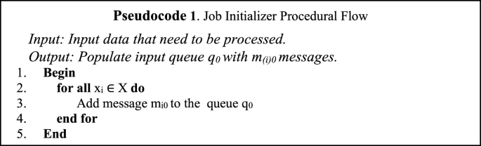
• 1. Job Initializer: Responsible for initiating the workflow’s first task by processing input data. Pseudocode 1 outlines the job initializer steps. It reads and extracts necessary details from the source data, creating messages in q₀ for each item. In the example of Fig. 4, the Job Initializer processes files f0 to fn in the source data repository, generating messages in queue q₀ containing the location details of the file. The first message for file f0 in queue q₀ is represented using m₍₀₎₀ where (0) in parenthesis represents the file number similarly for file f1 it is m₍₁₎₀.

  Fig. 4.

  

  ITS Execution and Data Flow

  

• 2. ITS: Responsible for scheduling the tasks in multiple job pools to ensure optimal utilization of resources at the task level. The ITS looks for messages in all the queues and schedules the tasks in the predicted job pool. Pseudocode 2 captures the steps in the ITS, which are explained below:

  • a. ITS keeps monitoring the queues for any messages. In Fig 4 the ITS is monitoring q₀ to q₅.

  • b. For the first task in the workflow, messages m_(f)0 are read from the queue q₀ after it is populated from the Job Initializer. In Fig. 4 the ITS will read messages m₍₀₎₀ to m_(n)0 from q_0.

  • c. For subsequent tasks message m_(f)i,j is read from the queue q_j populated from the task t_i. In Fig. 4, the ITS reads messages m_(0)0,1 to m_(n)0,1 from q₁ similarly from other queues such as m_(0)1,2 will read from q₂ and m_(0)2,3 will be read from q₃.

  • d. ITS checks the DAG in Fig. 3 to find parents for tasks t_j. If multiple parents exist, the queue q_j is searched for message m_(f)ij for all the parent task t_i using the unique task identifier m_index, and parent tasks t_i and merged before executing the task t_j. In example Fig. 4 the tasks t₀ to t₄ have single parents so message m_(f)0 is consumed by task t₀, m_(f)0,1 is consumed by task t₁, m_(f)2,3 is consumed by task t_3, and so on. In the case of q_5, task t₅ has parent t₄ and t₃ so the messages m_(f)4,5 and m_(f)3,5 are merged before executing t₅.

  • e. ITS identifies the best suitable VM Type required to run the task t_j.

  • f. ITS creates the task in the t_j job pool. The message data(md) in the message are passed as parameters to task t_j.

• 3. Task Executor: The Task Executor is responsible for executing and writing the output message back to the child task message queue for the next task execution. Pseudocode 3 captures the steps in the Task Executor. The flow involves consuming the parameters sent through message data md, executing the binaries associated with the task, and writing the results to the child task message queue. The following are the task executions that happen (see Fig. 4):

  

  

  • a. t0 (Document Download) downloads the file after reading the external file location in the message queue q0. The task stores the file in a common location in the local store and populates the message m0,1 in q1 and m0,2 in q2 with the location of the local store in the message.

  • b. t1 (Text Extraction) extracts the text from the document by reading the local file store location and populates the message q4 with the contents of the extracted text.

  • c. t2 (Image Extraction and OCR) extracts all the images from the document performs an OCR to extract the text and populates the message q3 with the contents of the extracted text.

  • d. t3 (Entity Extraction) extracts entities from the message received from t2 containing OCR text output and populates the message in q5 with the entities extracted.

  • e. t₄ (Text Summarization) summarizes the text output obtained from t₁ and populates the message in q₅ with the summarized text.

  • f. ITS merges the message data from t₂ containing entities extracted and t₄ containing the summarized text and triggers t₅.

  • g. t₅ (Database Update) updates the extracted information into the database.

5 Experimental Results

5.1 Dataset Details

We illustrate our approach for the Oil Industry domain to extract structured and unstructured data from images. The dataset was sourced from the BSEE website [15], an open repository of oil and gas industry data. The goal was to make images searchable based on text content and well-data attributes. The experiment involved processing 1000 images in Azure, involving tasks such as image download, classification, attribute extraction, OCR, NLP, and search index update. Figure 5 shows the image categories in the dataset.

Fig. 5.

Image Categories of Test Data Set

5.2 Azure Setup for the Experiment

Figure 6 shows the experimental setup in Azure [1].

• 1. Azure Storage: Azure blobs are used to store the images.

• 2. Processing Layer: Consists of Azure Batch and Scheduled Jobs. Azure Batch is a distributed computing PaaS platform provided by Azure and Schedule Jobs are services that run scripts on a schedule. They are configured to execute Job Initialization and ITS.

• 3. Search Layer: Consists of Azure cognitive search service that provides metadata and free text search from the extracted content.

• 4. ML Studio: Hosts the classification model that derives the VM size required for the task.

• 5. Forms Service: Used to extract structured data(attributes) from images. Figure 7 shows attributes such as well name, and lease name extracted from the forms services.

• 6. Custom Vision: Used for categorizing the images present in the source dataset, as shown in Fig. 5.

• 7. Storage Table: Used to store the log table containing the task compute node requirement.

Fig. 6.

Experimental setup of Azure Batch

Fig. 7.

Structured Data Extraction

5.3 Experiment Steps

The execution steps are:

• 1. Classifier Training: This step involved training the classifier model with training data containing the task resource requirements. Table 4 contains the training data with a compute node requirement column containing the Azure VM [1] size most suitable for running the task.

  Table 4. Classifier Training Data

• 2. Task Attribute Update: This step involved adding task attributes along with execution times into the storage table. Table 5 shows the entries in the Storage Table.

  Table 5. Task Attributes

• 3. Compute Node Prediction: Run the classification model against the entries in the table storage (Table 5) to determine the VM size required for running the tasks. Table 6 contains the compute node mapping obtained for each task in the Job. The entries in Table 6 are updated to the Storage Table for scheduling the tasks.

  Table 6. Task Compute Node Mapping

• 4. Run distributed Job using Azure Batch: The experiment involved creating two pools, Low-Cost Pool containing Standard_A4_v2 [16] (4 core, 8 GB RAM) VM and High-Cost Pool containing Standard_A8_v2 [16] (8 core, 16 GB RAM) VM. The number of machines used in the experiment was limited, considering the execution cost involved. The experiment involved three execution modes.

  • a) Low Cost – High Execution Time Approach: In this mode, we allocated three Standard_A4_v2 VMs in the Low Compute Pool and allocated the task of extracting data from 1000 images.

  • b) High Cost – Low Execution Time Approach: In this mode, we allocated three Standard_A8_v2 VMs in the High Compute Pool and allocated the task of extracting data from 1000 images.

  • c) ITS Approach: In this mode, we allocated two Standard_A1_v2 VMs in the Low Compute Pool and a single Standard_A8_v2 VM in the High Compute VM pool. We used the classification model to predict the task job pool. The allocation of tasks to the pool depended on the output of the prediction model and the number of jobs in the pool. If the job pool length is less than the threshold set to 10 tasks, any job will be allocated to the respective pool. The OCR extraction task was primarily allocated to the high compute pool, whereas all the other tasks were allocated to the low compute pool. This allocation procedure ensures that no processor is idle during the data extraction.

Table 7 shows the execution time in all three modes. There is an 8% decrease in execution time of the ITS Approach compared to the Low Cost- High Execution Time Approach and a total reduction of 68% in cost when the ITS Approach is compared with the High Cost – Low Execution Time Approach. The percentage reduction in time is calculated using the total execution time captured in Table 7. The total reduction in cost is obtained by multiplying the execution time with the unit price for VM usage from the Azure VM price sheet [16]. A similar experimental setup can be done on batch services provided by other CSPs such as AWS [17] and Google [18].

Table 7. Batch Execution Results

6 Conclusion

Distributed systems are computing platforms that can be used to handle large amounts of data processing. However, they can be costly depending on the time it takes to complete a job. This paper introduces a new framework that optimizes both the execution time and cost associated with running data processing tasks on a massive scale. The suggested technique includes the dynamic identification of the compute nodes to execute the task based on the classification model’s output. This model can be trained to optimize execution cost and execution time or additionally, it can be easily retrained with new parameters to enhance the system’s flexibility in accommodating new rules.

References

Directory of Azure Cloud Services | Microsoft Azure. https://azure.microsoft.com/en-in/products/
Chen, C.-Y., Huang, J.-J.: Double deep autoencoder for heterogeneous distributed clustering. Information 10(4), 144 (2019). https://doi.org/10.3390/info10040144
Pop, D., Iuhasz, G., Petcu, D.: Distributed platforms and cloud services: enabling machine learning for big data. In: Mahmood, Z. (ed.) Data Science and Big Data Computing, pp. 139–159. Springer, Cham (2016). https://doi.org/10.1007/978-3-319-31861-5_7
Nadeem, F., Alghazzawi, D., Mashat, A., Faqeeh, K., Almalaise, A.: Using machine learning ensemble methods to predict execution time of e-science workflows in heterogeneous distributed systems. IEEE Access 7, 25138–25149 (2019). https://doi.org/10.1109/ACCESS.2019.2899985
Sarnovsky, M., Olejnik, M.: Improvement in the efficiency of a distributed multi-label text classification algorithm using infrastructure and task-related data. Informatics 6(12), 1–15 (2019). https://doi.org/10.3390/informatics6010012
Ranjan, R.: Streaming big data processing in datacenter clouds, pp-78–83. IEEE Computer Society (2014)
Al-kahtani, M.S., Karim, L.: An efficient distributed algorithm for big data processing. Arab. J. Sci. Eng. 42(8), 3149–3157 (2017). https://doi.org/10.1007/s13369-016-2405-y
Bahnasawy, N.A., Omara, F., Koutb, M.A., Mosa, M.: Optimization procedure for algorithms of task scheduling in high performance heterogeneous distributed computing systems. Egypt. Inform. J. 12(3), 219–229 (2011). https://doi.org/10.1016/j.eij.2011.10.001. ISSN 1110-8665
Jahanshahi, M., Meybodi, M.R., Dehghan, M.: A new approach for task scheduling in distributed systems using learning automata. In: 2009 IEEE International Conference on Automation and Logistics, pp. 62–67 (2009). https://doi.org/10.1109/ICAL.2009.5262978
Sriraman, A., Dhanotia, A., Wenisch, T.F.: SoftSKU: optimizing server architectures for microservice diversity @scale. In: 2019 ACM/IEEE 46th Annual International Symposium on Computer Architecture (ISCA), pp. 513–526 (2019)
Pandey, R., Silakari, S.: Investigations on optimizing performance of the distributed computing in heterogeneous environment using machine learning technique for large scale data set. Mater. Today: Proc. (2021). https://doi.org/10.1016/j.matpr.2021.07.089. ISSN 2214-7853
Optical character recognition. https://en.wikipedia.org/wiki/Optical_character_recognition
Entity Extraction. https://en.wikipedia.org/wiki/Named-entity_recognition
Directed acyclic graph – Wikipedia. https://en.wikipedia.org/wiki/Directed_acyclic_graph
Scanned Well Files Query. https://www.data.bsee.gov/Other/DiscMediaStore/ScanWellFiles.aspx
Pricing - Windows Virtual Machines | Microsoft Azure. https://azure.microsoft.com/en-in/pricing/details/virtual-machines/windows/
Getting Started with AWS Batch - AWS Batch. https://docs.aws.amazon.com/batch/latest/userguide/Batch_GetStarted.html#first-run-step-2
Batch service on Google Cloud. https://cloud.google.com/blog/products/compute/new-batch-service-processes-batch-jobs-on-google-cloud
Author information
Authors and Affiliations
Corresponding author
Editor information
Editors and Affiliations
Rights and permissions
Copyright information
© 2024 The Author(s), under exclusive license to Springer Nature Switzerland AG
About this paper
Cite this paper
Venkatesh, P.R., Radha Krishna, P. (2024). An Improved and Efficient Distributed Computing Framework with Intelligent Task Scheduling. In: Devismes, S., Mandal, P.S., Saradhi, V.V., Prasad, B., Molla, A.R., Sharma, G. (eds) Distributed Computing and Intelligent Technology. ICDCIT 2024. Lecture Notes in Computer Science, vol 14501. Springer, Cham. https://doi.org/10.1007/978-3-031-50583-6_2
Download citation
DOI: https://doi.org/10.1007/978-3-031-50583-6_2
Published:
Publisher Name: Springer, Cham
Print ISBN: 978-3-031-50582-9
Online ISBN: 978-3-031-50583-6
eBook Packages: Computer ScienceComputer Science (R0)