Randomized Functions with High Round Complexity

Abstract

Consider two-party secure function evaluation against an honest-but-curious adversary in the information-theoretic plain model. We study the round complexity of securely realizing a given secure function evaluation functionality.

Chor-Kushilevitz-Beaver (1989) proved that the round complexity of securely evaluating a deterministic function depends solely on the cardinality of its domain and range. A natural conjecture asserts that this phenomenon extends to functions with randomized output.

Our work falsifies this conjecture – revealing intricate subtleties even for this elementary security notion. For every r, we construct a function $f_r$ with binary inputs and five output alphabets that has round complexity r. Previously, such a construction was known using $(r+1)$ output symbols. Our counter-example is optimal – we prove that any securely realizable function with binary inputs and four output alphabets has round complexity at most four.

We work in the geometric framework Basu-Khorasgani-Maji-Nguyen (FOCS–2022) introduced to investigate randomized functions’ round complexity. Our work establishes a connection between secure computation and the lamination hull (geometric object originally motivated by applications in hydrodynamics). Our counterexample constructions are related to the “tartan square” construction in the lamination hull literature.

H. H. Nguyen—This work was done while the author was at Purdue.

Basu was partially supported by NSF grants CCF-1910441 and CCF-2128702. Khorasgani, Maji, and Nguyen are supported in part by an NSF CRII Award CNS–1566499, NSF SMALL Awards CNS–1618822 and CNS–2055605, the IARPA HECTOR project, MITRE Innovation Program Academic Cybersecurity Research Awards (2019–2020, 2020–2021), a Ross-Lynn Research Scholars Grant, a Purdue Research Foundation (PRF) Award, and The Center for Science of Information, an NSF Science and Technology Center, Cooperative Agreement CCF–0939370.

1 Introduction

Secure multi-party computation (MPC) [13, 18] allows mutually distrusting parties to compute securely over their private data. In general, MPC requires an honest majority or oblivious transfer to compute tasks securely. Even if honest parties are not in the majority, several tasks are securely computable in the information-theoretic plain model without oblivious transfer or other hardness of computation assumptions. For example, the Dutch auction mechanism [6] securely performs auctions. These information-theoretic protocols, if they exist, are highly desirable – they are perfectly secure, fast, and require no setup or preprocessing. With rapid increases in the computational power of parties, the round complexity of these protocols becomes the primary bottleneck, significantly impacting their adoption.

This work studies the round complexity of MPC in the two-party information-theoretic plain model against honest-but-curious adversaries. Alice and Bob have private inputs $x\in X$ and $y\in Y$, respectively, and their objective is to securely sample an output z from the distribution f(x, y) over the sample space Z. The distribution f(x, y) is publicly known, and both parties must receive the identical output z. Parties have unbounded computational power and honestly follow the protocol; however, they are curious to obtain additional information about the other party’s private input. An ideal communication channel connects the parties, and they send messages in alternating rounds.¹ The round complexity of securely computing f is the (worst-case) minimum number of rounds required to perform this sampling task securely.

We aim to investigate factors causing high round complexity for these secure sampling tasks. Increasing the size of the input or output sets would certainly lead to higher round complexity. However, even after fixing the input and output sets, the complexity of representing the probability distributions could influence the round complexity. There is a natural conjecture in this context.

It is conjectured that only the sizes of the input and output sets determine the round complexity. The complexity of representing the probability distributions f(x, y) is absorbed within the private computation that parties perform, and it does not impact the round complexity.

This (extremely strong) conjecture is known to hold for (a) classical communication complexity where correctness (not security) is considered, (b) the secure computation tasks with deterministic output, and (c) randomized output tasks with a small output set. In the sequel, Sect. 1.1, Sect. 1.2, and Sect. 1.4 present evidence supporting the credibility of this conjecture. Our work refutes this conjecture. Section 2 presents our contributions and Sect. 3 highlights the underlying technical approach.

1.1 Discussion: Interaction in a World Without Security

Consider the classical communication complexity objective of correctly (possibly insecurely) evaluating a randomized output function with minimum interaction. In this context, the following canonical interactive protocol is natural. Alice sends her input x to Bob. Bob samples $z\sim f(x,y)$ and sends the output z to Alice.² The round complexity of this (insecure) protocol is two. More generally, its communication complexity is $\log \textrm{card}\left( X\right) +\log \textrm{card}\left( Z\right)$, where $\textrm{card}\left( S\right)$ represents the cardinality of the set S. These upper bounds on the interaction complexity hold irrespective of the complexity of representing the individual probabilities $f(x,y)_z$, the probability to output $z\in Z$ conditioned on the input $(x,y)\in X\times Y$. The computational complexity of sampling their output did not overflow into the interaction complexity because its impact was contained within the respective parties’ private computation.

1.2 Round Complexity of Deterministic Functions

A particular class of functions widely studied in communication complexity and cryptography is the class of deterministic functions. The function f is deterministic if the support of the distribution f(x, y) is a singleton set for every $(x,y)\in X\times Y$ – the output z is determined entirely by the parties’ private inputs (x, y). For example, in an auction, the price is determined by all the bids.

Chor-Kushilevitz-Beaver [4, 8, 17] characterized all deterministic functions that are securely computable in the two-party information-theoretic plain model against honest-but-curious adversaries. The secure protocols for such functions follow a general template – parties rule out specific outputs in each round. Excluding outputs, in turn, rules out private input pairs (because each input pair produces one output). For example, the Dutch auction mechanism rules out the price that receives no bids. Such functions are called decomposable functions because these secure protocols incrementally decompose the feasible input-output space during their evolution. Decomposable functions are securely computable with perfect security.

Let us reason about the round complexity of a deterministic function $f:X\times Y\rightarrow Z$, represented by $\textrm{round}\left( f\right)$. One has to exclude $\textrm{card}\left( Z\right) -1$ outputs so that only the output $z=f(x,y)$ remains feasible. So, if f has a secure protocol in this model, then

$$ \textrm{round}\left( f\right) \leqslant \textrm{card}\left( Z\right) -1.$$

Furthermore, the Markov property for interactive protocols holds in the information-theoretic plain model. The joint distribution of inputs conditioned on the protocol’s evolution is always a product distribution. Excluding output also excludes private inputs of the parties. For example, if Alice sends a message in a round, she rules out some of her private inputs. This observation leads to the bound

$$ \textrm{round}\left( f\right) \leqslant 2\cdot \textrm{card}\left( X\right) -1.$$

Likewise, we also have

$$ \textrm{round}\left( f\right) \leqslant 2\cdot \textrm{card}\left( Y\right) -1.$$

Combining these observations, Chor-Kushilevitz-Beaver [4, 8, 17] concluded that

$$\begin{aligned} \textrm{round}\left( f\right) \leqslant \min \left\{ \textrm{card}\left( Z\right) , 2\cdot \textrm{card}\left( X\right) , 2\cdot \textrm{card}\left( Y\right) \right\} - 1. \end{aligned}$$

(1)

The cardinalities of the private input and output sets determine the upper bound on the round complexity of f if it has a secure protocol. This phenomenon from the classical communication complexity extends to the cryptographic context for deterministic functions.

1.3 Round Complexity of Randomized Functions with Small Output Set

For functions with randomized output, the first conjecture already holds for small values of $\textrm{card}\left( Z\right)$. For example, $\textrm{card}\left( Z\right) \leqslant 3$ implies that $\textrm{round}\left( f\right) \leqslant 2$ [11]. In fact, this paper will prove that $\textrm{card}\left( Z\right) \leqslant 4$ implies $\textrm{round}\left( f\right) \leqslant 4$. It is fascinating that the complexity of sampling from the distributions f(x, y) does not impact the round complexity; its role is localized to the parties’ private computation.

1.4 Round Complexity of Randomized Functions (General Case)

For three decades, there was essentially no progress in determining the round complexity of securely computing general randomized functions – barring a few highly specialized cases [11]. Last year, Basu, Khorasgani, Maji, and Nguyen (FOCS 2022) [1] showed that determining “whether a randomized f has an r-round protocol or not” is decidable. They reduced this question to a geometric analog: “does a query point Q belong to a recursively-generated set $\mathcal S ^{\left( r\right) }$.” They start with an initial set of points $\mathcal S ^{\left( 0\right) }$, and recursively build $\mathcal S ^{\left( i+1\right) }$ from the set $\mathcal S ^{\left( i\right) }$ using a geometric action, for $i\in \{0,1,\dotsc \}$. The function f has an (at most) r-round protocol if (and only if) a specific query point Q belongs to the set $\mathcal S ^{\left( r\right) }$.

These set of points $\left\{ \mathcal S ^{\left( i\right) } \right\} _{i\geqslant 0}$ lie in the ambient space

$$ \mathbb {R}^{\textrm{card}\left( X\right) -1} \times \mathbb {R}^{\textrm{card}\left( Y\right) -1} \times \mathbb {R}^{\textrm{card}\left( Z\right) }.$$

Again, the dimension of the ambient space (of their embedding) is determined entirely by the cardinalities of the inputs and output sets. This feature of their embedding added additional support to the conjecture.

Consider an analogy from geometry. Consider n initial points in $\mathbb {R}^d$, where $n \gg d$. At the outset, any point inside the convex hull can be expressed as a convex linear combination of the initial points that lie on the convex hull; their number can be $\gg d$. However, Carathéodory ’s theorem [7] states that every point in its interior is expressible as a convex linear combination of (at most) $(d+1)$ initial points on the convex hull. At an abstract level: canonical representations may have significantly lower complexity. It is similar to the Pumping lemma for regular languages and (more generally) the Ogden lemma for context-free languages.

Likewise, a fascinating possibility opens up in the context of Basu et al. ’s geometric problem. The canonical protocol for f could have round complexity determined solely by the dimension of their ambient space, which (in turn) is determined by the cardinality of the input and output sets. In fact, an optimistic conjecture of $\mathcal {O}\left( {\textrm{card}\left( Z\right) ^2}\right)$ upper bound on the round complexity appears in the full version of their paper [2, Section 7, Conjecture 1].

We Refute This Conjecture. The analogies break exactly at $\left|Z \right|=5$. Represent a randomized function with input set $X\times Y$ and output set Z as $f:X\times Y\rightarrow \mathbb {R}^Z$. For every $r\in \{1,2,\dotsc \}$, we construct a function $f_r:\{0,1\}\times \{0,1\}\rightarrow \mathbb {R}^{\{1,2,3,4,5\}}$ with round complexity r. Previously, Basu et al. constructed functions $g_r :\{0,1\}\times \{0,1\}\rightarrow \mathbb {R}^{\{1,2,\dotsc ,r+1\}}$ with round complexity r, i.e., their example had $\textrm{card}\left( Z\right) =(r+1)$. In our example, $\textrm{card}\left( Z\right) =5$, a constant. Moreover, we prove the optimality of the counterexamples: Any $f:\{0,1\}\times \{0,1\}\rightarrow \mathbb {R}^{\{1,2,3,4\}}$ has round complexity $\leqslant 4$.

Looking Ahead. Our results indicate that any upper bound on the round complexity of f must involve the complexity of representing (the probabilities appearing in) the function f. For example, consider a randomized function whose probabilities are integral multiples of 1/B. Then, the round complexity of f should be upper bounded by some function of $\textrm{card}\left( X\right)$, $\textrm{card}\left( Y\right)$, $\textrm{card}\left( Z\right)$, and B. The B-term represents (intuitively) “the condition number of the function f.” If this dependence on B can, in fact, be a $\textsf{poly}{\left( \log (B)\right) }$ dependence, then it will lead to efficient secure algorithms, ones with round complexity of $\textsf{poly}{\left( \log B\right) }$.

Our work considers the round complexity of perfectly secure protocols. The case of statistically secure protocols remains an interesting open problem. In fact, the decidability of the question: “Is there an r-round $\varepsilon$-secure protocol for f?” remains unknown, which is a more fundamental problem. Basu et al.  [1] only considered the perfect security case. The technical machinery to handle statistical security for general randomized output functions does not exist. This work does not contribute to these two research directions.

1.5 Overview of the Paper

We discuss our contributions in Sect. 2. In Sect. 3, we provide a technical overview of our paper. In Sect. 4, we discuss the relation of our work with lamination hull. Section 5 presents the BKMN geometric framework. Section 6 introduces notations and preliminaries. Section 7 contains all results pertaining to constructing high-round complexity randomized functions. Section 8 shows that our counterexamples are optimal.

2 Our Contributions

Theorem 1

(Functions with arbitrarily high round complexity). For any $r \in \{1,2,\dotsc , \}$, there is a function $f_r:\{0,1\} \times \{0,1\} \rightarrow {\mathbb {R}} ^{\{1,2,3,4,5\}}$ such that $\textrm{round}\left( f_r\right) =r$.

The function $f_r$ has an r-round perfectly secure protocol (and r bits of communication) but no $(r-1)$-round perfectly secure protocol. This result proves that there are functions with arbitrary large round complexity with a constant input and output set size. Previously, Basu et al.  [1] constructed functions with high round complexity with $(r+1)$ output alphabets. This result is a counterexample to the folklore conjecture. Section 7 presents the definition of the functions and the proof.

Our counterexample is also optimal, which is a consequence of our following result.

Theorem 2

(Bounded Round Complexity for $\textrm{card}\left( Z\right) \leqslant 4$). Any function $f :\{0,1\}\times \{0,1\}\rightarrow \mathbb {R}^Z$ with $\textrm{card}\left( Z\right) \leqslant 4$ has $\textrm{round}\left( f\right) \leqslant 4$.

Section 8 proves this theorem.

3 Technical Overview of Our Results

The presentation in this work is entirely geometric. No background in security is necessary. We use the geometric embedding of BKMN [1] to translate round complexity problems into geometric problems. Security is already folded inside their geometric embedding.

3.1 High-Level Summary of the BKMN Geometric Framework

Section 5 presents a detailed version of this section. Consider a randomized output function $f:\{0,1\}\times \{0,1\}\rightarrow \mathbb {R}^ Z$. BKMN approach considers the ambient space $\mathbb {R}^d$, where $d=\textrm{card}\left( Z\right) + 2$. They present the following maps

• 1. Function encoding. $f \mapsto (A,B,V)$, where the matrix $A\in \mathcal M _{2\times \textrm{card}\left( Z\right) }(\mathbb {R})$³, the matrix $B\in \mathcal M _{2\times \textrm{card}\left( Z\right) }(\mathbb {R})$, and the vector $V\in \mathbb {R}^{\textrm{card}\left( Z\right) }$

• 2. Query point. $f \mapsto Q(f) \in \mathbb {R}^{\textrm{card}\left( Z\right) }$

• 3. Initial set. $(A,B) \mapsto \mathcal S ^{\left( 0\right) } \subseteq \mathbb {R}^d$ satisfying $\textrm{card}\left( \mathcal S ^{\left( 0\right) } \right) =\textrm{card}\left( Z\right)$.

They present the following recursive definition of $\mathcal S ^{\left( i+1\right) } \subseteq \mathbb {R}^d$ from $\mathcal S ^{\left( i\right) } \subseteq \mathbb {R}^d$, for all $i\in \{0,1,\dotsc \}$.

$$ \mathcal S ^{\left( i+1\right) } = \left\{ \sum _{k=1}^t \lambda ^{\left( k\right) } \cdot Q^{\left( k\right) } \;:\; \begin{matrix} t\in \{1,2,\dotsc \}, \\ \lambda ^{\left( 1\right) }, \lambda ^{\left( 2\right) }, \dotsc , \lambda ^{\left( t\right) } \geqslant 0, \\ \lambda ^{\left( 1\right) } + \lambda ^{\left( 2\right) } + \cdots + \lambda ^{\left( t\right) } = 1, \\ Q^{\left( 1\right) }, Q^{\left( 2\right) }, \dotsc , Q^{\left( t\right) } \in \mathcal S ^{\left( i\right) }, \text { and} \\ \left( Q^{\left( 1\right) } _1 = Q^{\left( 2\right) } _1 = \cdots = Q^{\left( t\right) } _1\text { or } \right. \\ \left. Q^{\left( 1\right) } _2 = Q^{\left( 2\right) } _2 = \cdots = Q^{\left( t\right) } _2\right) \end{matrix}\right\} .$$

Intuitively, this recursive definition ensures the following. Pick any t points $Q^{\left( 1\right) }, Q^{\left( 2\right) }, \dotsc , Q^{\left( t\right) } \in \mathcal S ^{\left( i\right) }$, where $t\in \{1,2,\dotsc \}$. If the first coordinates of all these t points are identical, or the second coordinates of all these t points are identical, then add all possible convex linear combinations (i.e., the convex hull) of $\left\{ Q^{\left( 1\right) }, Q^{\left( 2\right) }, \dotsc , Q^{\left( t\right) } \right\}$ to the set $\mathcal S ^{\left( i+1\right) }$.

Remark 1

(Communication complexity). Restricting the recursive definition to $t=2$ corresponds to investigating the communication complexity of f. This version of the recursion is closely connected to the lamination hull defined in Sect. 4.

Observe that, in the recursive definition, the points need not be distinct. Therefore, choosing $Q^{\left( 1\right) } =Q^{\left( 2\right) } =\cdots =Q^{\left( t\right) }$ ensures that $\mathcal S ^{\left( i\right) } \subseteq \mathcal S ^{\left( i+1\right) }$. Using this recursive definition, we have the following sequence of sets in $\mathbb {R}^d$:

$$ \mathcal S ^{\left( 0\right) } \subseteq \mathcal S ^{\left( 1\right) } \subseteq \mathcal S ^{\left( 2\right) } \subseteq \cdots $$

Connection to Round Complexity of Secure Computation. BKMN [1] proved that, for all $r\in \{0,1,\dotsc \}$, $\textrm{round}\left( f\right) \leqslant r$ if and only if $Q(f) \in \mathcal S ^{\left( r\right) }$. Therefore, to prove $\textrm{round}\left( f\right) =r$, it suffices to prove that $Q(f)\in \mathcal S ^{\left( r\right) } \setminus \mathcal S ^{\left( r-1\right) }$.

3.2 The “Tartan Square” Meets Secure Computation

Our objective is to prove that there is a function $f_r:\{0,1\}\times \{0,1\}\rightarrow \mathbb {R}^Z$, where $Z=\{1,2,\dotsc ,5\}$, such that $f_r\in \mathcal S ^{\left( r\right) } \setminus \mathcal S ^{\left( r-1\right) }$, for every $r\in \{1,2,\dotsc \}$. Recall that $\mathcal S ^{\left( 0\right) }$ is determined by $f_r$ and $\textrm{card}\left( \mathcal S ^{\left( 0\right) } \right) =\textrm{card}\left( Z\right) =5$. Furthermore, all the sets $\mathcal S ^{\left( i\right) }$ are in ambient space $\mathbb {R}^7$, for $i\in \{0,1,\dotsc \}$.

A preliminary step towards designing such functions is to determine an initial set of points $\mathcal S ^{\left( 0\right) }$ such that we have

$$ \mathcal S ^{\left( 0\right) } \subsetneq \mathcal S ^{\left( 1\right) } \subsetneq \mathcal S ^{\left( 2\right) } \subsetneq \cdots $$

Otherwise, suppose $\mathcal S ^{\left( i\right) } = \mathcal S ^{\left( i+1\right) }$, for some $i\in \{0,1,\dotsc \}$. Then, $\mathcal S ^{\left( j\right) } =\mathcal S ^{\left( i\right) }$, for all $j\geqslant i$, and the round complexity cannot surpass i. So, our objective is to construct an initial set $\mathcal S ^{\left( 0\right) }$ of constant size in an ambient space of constant dimension such that the evolution of the sequence $\mathcal S ^{\left( 0\right) } \rightarrow \mathcal S ^{\left( 1\right) } \rightarrow \mathcal S ^{\left( 2\right) } \rightarrow \cdots$ does not stabilize. It is unclear whether such an initial set $\mathcal S ^{\left( 0\right) }$ even exists.

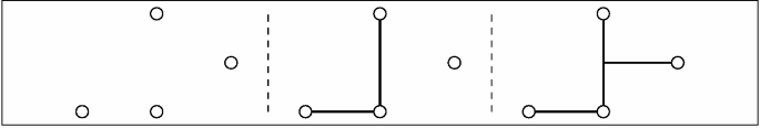
Illustrative Example. We present an initial set $\mathcal S ^{\left( 0\right) } \subseteq \mathbb {R}^3$ such that the evolution of the recursively defined sets does not stabilize. We emphasize that this illustrative example is for intuition purposes only. The actual constructions are presented in Sect. 7, where the ambient space is $\mathbb {R}^7$.

We work in the ambient space $\mathbb {R}^3$ for the illustrative example. Consider an initial set of points

$$ \mathbb {R}^3 \supseteq \mathcal S ^{\left( 0\right) } \;:=\; \Big \{ (2,0,0), \; (0,1,0), \; (1,3,0), \; (3,2,0), \; (2,1,1) \Big \} $$

• 1. For example, consider the points (0, 1, 0) and (2, 1, 1) in the set $\mathcal S ^{\left( 0\right) }$. The recursive definition allows the addition of the line segment $\overline{PQ}$ to the set $\mathcal S ^{\left( 1\right) }$. In particular, this line segment’s midpoint (1, 1, 1/2) is in the set $\mathcal S ^{\left( 1\right) }$.

• 2. Similarly, considering the points (1, 3, 0) and (1, 1, 1/2) in the set $\mathcal S ^{\left( 1\right) }$, we conclude that their midpoint (1, 2, 1/4) is in the set $\mathcal S ^{\left( 2\right) }$.

• 3. Now, consider the points (3, 2, 0) and (1, 2, 1/4) in the set $\mathcal S ^{\left( 2\right) }$. Their midpoint (2, 2, 1/8) is in the set $\mathcal S ^{\left( 3\right) }$.

• 4. Finally, the midpoint of the points (2, 0, 0) and (2, 2, 1/8) in the set $\mathcal S ^{\left( 3\right) }$ is (2, 1, 1/16), which is in the set $\mathcal S ^{\left( 4\right) }$.

Let us summarize what we have achieved thus far. Beginning with the point $(2,1,1)\in \mathcal S ^{\left( 0\right) }$, we identified the point $(2,1,1/16)\in \mathcal S ^{\left( 4\right) }$. One can prove that this point $(2,1,1/16) \not \in \mathcal S ^{\left( 3\right) }$. Therefore, we conclude that the point $(2,1,1/16)\in \mathcal S ^{\left( 4\right) } \setminus \mathcal S ^{\left( 3\right) }$.

Using analogous steps as above, starting instead with the point $(2,1,1/16)\in \mathcal S ^{\left( 4\right) } \setminus \mathcal S ^{\left( 3\right) }$ will lead to the point $\left( 2,1,1/(16)^2 \right) \in \mathcal S ^{\left( 8\right) } \setminus \mathcal S ^{\left( 7\right) }$ In general, using this construction, we will have

$$ \left( 2, 1, \frac{1}{16^k} \right) \in \mathcal S ^{\left( 4k\right) } \setminus \mathcal S ^{\left( 4k-1\right) }.$$

This sequence of points, for $k\in \{0,1,2,\dotsc \}$, demonstrate that the sequence $\mathcal S ^{\left( 0\right) } \rightarrow \mathcal S ^{\left( 1\right) } \rightarrow \mathcal S ^{\left( 2\right) } \rightarrow \cdots$ does not stabilize. This example is the “tartan square” from the lamination hull literature; refer to Remark 2 in Sect. 4.

This illustrative example leads to the following conclusion. In an ambient space of constant dimension and starting with a suitable initial set $\mathcal S ^{\left( 0\right) }$ of constant size, the sequence $\mathcal S ^{\left( 0\right) } \rightarrow \mathcal S ^{\left( 1\right) } \rightarrow \mathcal S ^{\left( 2\right) } \rightarrow \cdots$ may not stabilize.

3.3 Overview: Proof of Theorem 1

For $r\in \{1,2,\dotsc \}$, we will appropriately choose the probabilities of the function $f_r:\{0,1\}\times \{0,1\}\rightarrow \mathbb {R}^Z$, such that $\textrm{card}\left( Z\right) =5$. Using the BKMN geometric framework (see Sect. 3.1), we will generate:

• 1. Function encoding $(A,B,V_r)$. We emphasize that all our functions $f_r$ are designed so that they map to the same (A, B); only $V_r$ is different.

• 2. Query point $Q(f_r)\in \mathbb {R}^7$.

• 3. Initial point set $\mathcal S ^{\left( 0\right) } \subseteq \mathbb {R}^7$, which is identical for all $f_r$ because (a) all functions map to identical (A, B), and (b) (A, B) alone determine $\mathcal S ^{\left( 0\right) }$.

Sect. 5.1 presents the definition of the function $f_r$.

Next, the choice of the $\mathcal S ^{\left( 0\right) }$ ensures that the evolution of the sets $\mathcal S ^{\left( 0\right) } \rightarrow \mathcal S ^{\left( 1\right) } \rightarrow \mathcal S ^{\left( 2\right) } \rightarrow \cdots$ does not stabilize. It essentially mimics the tartan square construction of Sect. 3.2. However, we emphasize that in this section, the ambient space is $\mathbb {R}^7$ (the ambient space for the tartan square example was $\mathbb {R}^3$). Furthermore, we design our function $f_r$ such that the corresponding query point $Q(f_r) \in \mathcal S ^{\left( r\right) } \setminus \mathcal S ^{\left( r-1\right) }$. Consequently, we have $\textrm{round}\left( f_r\right) =r$.

3.4 Overview: Proof of Theorem 2

We aim to prove that $\textrm{round}\left( f\right) \leqslant 4$, for any function $f:\{0,1\}\times \{0,1\}\rightarrow \mathbb {R}^Z$ such that $\textrm{card}\left( Z\right) \leqslant 4$. Toward this objective, we begin with the following observations.

• 1. Recall that in the BKMN framework $\textrm{card}\left( \mathcal S ^{\left( 0\right) } \right) =\textrm{card}\left( Z\right)$.

• 2. Furthermore, if $\mathcal S ^{\left( 4\right) } = \mathcal S ^{\left( 5\right) }$, then $\mathcal S ^{\left( j\right) } =\mathcal S ^{\left( 4\right) }$, for all $j\geqslant 4$. In this case, $\textrm{round}\left( f\right) \leqslant 4$, because $\mathcal S ^{\left( r\right) } \setminus \mathcal S ^{\left( r-1\right) } =\emptyset$, for all $r\in \{5,6,\dotsc \}$.

To prove our theorem, it will suffice to prove that the evolution of the sets $\mathcal S ^{\left( 0\right) } \rightarrow \mathcal S ^{\left( 1\right) } \rightarrow \mathcal S ^{\left( 2\right) } \rightarrow \cdots$ stabilizes by $i=4$ when $\textrm{card}\left( \mathcal S ^{\left( 0\right) } \right) \leqslant 4$.⁴ We prove this result using an exhaustive case analysis (see Sect. 8).

4 Lamination Hull

Consider an ambient space $\mathbb {R}^d$. The lamination hull is parameterized by a set of points $\varLambda \subseteq \mathbb {R}^d$. Given a set of initial point $\mathcal S ^{\left( 0,\varLambda \right) } \subseteq \mathbb {R}^d$, recursively define $\mathcal S ^{\left( i+1,\varLambda \right) }$ from $\mathcal S ^{\left( i\right) }$ as follows

$$ \mathcal S ^{\left( i+1,\varLambda \right) } \;:=\; \left\{ \lambda \cdot Q^{\left( 1\right) } + (1-\lambda )\cdot Q^{\left( 2\right) } :\begin{matrix} Q^{\left( 1\right) },Q^{\left( 2\right) } \in \mathcal S ^{\left( i,\varLambda \right) },\\ \lambda \in [0,1],\text { and}\\ Q^{\left( 1\right) }-Q^{\left( 2\right) } \in \varLambda \end{matrix} \right\} .$$

Intuitively, one can add the line segment $\overline{Q^{\left( 1\right) } Q^{\left( 2\right) }}$ to the set $\mathcal S ^{\left( i+1,\varLambda \right) }$ for any $Q^{\left( 1\right) },Q^{\left( 2\right) } \in \mathcal S ^{\left( i,\varLambda \right) }$ if $Q^{\left( 1\right) }-Q^{\left( 2\right) } \in \varLambda$. The lamination hull is the limit of the sequence $\mathcal S ^{\left( 0,\varLambda \right) } \rightarrow \mathcal S ^{\left( 1,\varLambda \right) } \rightarrow \mathcal S ^{\left( 2,\varLambda \right) } \rightarrow \cdots$. This hull is tied to computing the stationary solutions to the following differential equations underlying incompressible porous media [9, 10, 12, 14].

When $\varLambda = (0,\mathbb {R},\dotsc ,\mathbb {R}) \cup (\mathbb {R},0,\mathbb {R},\dotsc ,\mathbb {R}) \subseteq \mathbb {R}^d$, the sequence $\mathcal S ^{\left( 0,\varLambda \right) } \rightarrow \mathcal S ^{\left( 1,\varLambda \right) } \rightarrow \mathcal S ^{\left( 2,\varLambda \right) } \rightarrow \cdots$ is identical to the sequence defined by Basu et al.  [1] for the communication complexity case (see Remark 1). Basu et al.  [1] proved that the points in the recursively defined sets are related to secure computation protocols. As a consequence of this connection, secure computation protocols manifest in physical processes in nature. This connection is mentioned in [3, Page 20].

Remark 2

(Independent discovery of the “tartan square” construction). Our work independently discovered the “tartan square” construction in the lamination hull literature [16, Figure 2, Page 3]. Consider ambient dimension $\mathbb {R}^3$ and $\varLambda = (0,\mathbb {R},\mathbb {R}) \cup (\mathbb {R},0,\mathbb {R})\subseteq \mathbb {R}^d$. The “tartan square” is a set of 5 points in $\mathbb {R}^3$ such that the sequence $\mathcal S ^{\left( 0,\varLambda \right) } \rightarrow \mathcal S ^{\left( 1,\varLambda \right) } \rightarrow \mathcal S ^{\left( 2,\varLambda \right) } \rightarrow \cdots$ does not stabilize. Section 3 uses this example to provide the intuition underlying our counterexample constructions.

5 BKMN Geometric Framework: A Formal Introduction

Basu-Khorasgani-Maji-Nguyen [1] presents a new approach for studying the round complexity of any (symmetric) functionality $f :X \times Y \rightarrow \mathbb {R}^Z$. In the following discussion, we shall recall this approach for the particular case where the input domain satisfies $X = Y = \{0,1\}$.

From the given functionality f, BKMN22 defines the following maps.

• 1. Function encoding: $f \mapsto (A,B,V)$

• 2. Query point: $f \mapsto Q(f)$

• 3. Initial set: $(A,B) \mapsto \mathcal S ^{\left( 0\right) }$

• 4. Recursive construction: $\mathcal S ^{\left( i\right) } \mapsto \mathcal S ^{\left( i+1\right) }$ for any $i\in \{0,1,2,\dotsc \}$.

The query point Q(f) is constructed as follows.

The initial set $\mathcal S ^{\left( 0\right) }$ is constructed from (A, B) as follows.

They consider the sequence $\mathcal S ^{\left( 0\right) }, \mathcal S ^{\left( 1\right) },\dotsc ,\mathcal S ^{\left( i\right) }, \dotsc$ where for any $i \in \{0,1,\dotsc \}$, the geometric action that recursively generates $\mathcal S ^{\left( i+1\right) }$ from $\mathcal S ^{\left( i\right) }$ is defined as follows:

Some Clarifications.

• 1. A convex linear combination of the points $Q^{\left( 1\right) }, \dotsc , Q^{\left( t\right) }$, is a point of the form $\lambda ^{\left( 1\right) } \cdot Q^{\left( 1\right) } + \cdots + \lambda ^{\left( t\right) } \cdot Q^{\left( t\right) }$, where $\lambda ^{\left( 1\right) },\dotsc ,\lambda ^{\left( t\right) } \geqslant 0$ and $\sum \limits _{i=1}^t \lambda ^{\left( i\right) } =1$. All possible convex linear combinations consider all possible such $\lambda ^{\left( 1\right) },\dotsc \lambda ^{\left( t\right) }$ values.

• 2. The points $Q^{\left( 1\right) },\dotsc ,Q^{\left( t\right) }$ in the definition need not be distinct

• 3. Considering $t=1$ in the definition above ensures that $\mathcal S ^{\left( i\right) } \subseteq \mathcal S ^{\left( i+1\right) }$.

• 4. Since efficiency is not a consideration in the current context, we consider $t\in \{1,2,\dotsc \}$. Otherwise, by Carathéodory ’s theorem [7], it suffices to consider only $t=(d+1)$.

BKMN’s Reduction. Given the initial set $\mathcal S ^{\left( 0\right) }$, one constructs the sequence $\mathcal S ^{\left( 0\right) } \rightarrow \mathcal S ^{\left( 1\right) } \rightarrow \mathcal S ^{\left( 2\right) } \rightarrow \dotsc$ recursively based on the geometric action. Basu et al. reduce the problem of the round complexity of secure computation of randomized functions to the problem of testing whether a point belongs to a set in a high dimensional space.

5.1 An Example

In this section, we consider an example and find the corresponding encoding, query point, and sets $\mathcal S ^{\left( 0\right) }, \mathcal S ^{\left( 1\right) },\dots$ based on BKMN’s approach. For any $r = 4k+1$ where $k\in \{0,1,\dotsc \}$, we construct a functionality $f_r :\{0,1\}\times \{0,1\}\rightarrow \mathbb {R}^{\{1,2,3,4,5\}}$ and then show in Sect. 7 that $\textrm{round}\left( f_r\right) = r$. We emphasize that it is also possible to construct such functionality for the cases that $r=4k$ or $r=4k+2$ or $r=4k+3$ where $k\in \{0,1,2,\dotsc \}$.

Consider the following functionality

$$\begin{aligned} &f_{4k+1}(0,0)=\left( \frac{3}{16}\cdot \sigma _k, \; \frac{1}{4}\cdot \sigma _{k+1},\; \frac{1}{8}\cdot \sigma _k,\; \frac{3}{8}\cdot \sigma _k,\; \frac{3}{2^{4k+2}}\right) ,\\ &f_{4k+1}(0,1)=\left( \frac{9}{16}\cdot \sigma _k,\; \frac{1}{4} \cdot \sigma _{k+1}, \;\; 0\cdot \sigma _k,\;\frac{1}{8}\cdot \sigma _k, \;\frac{3}{2^{4k+2}}\right) ,\\ &f_{4k+1}(1,0)=\left( \frac{1}{16}\cdot \sigma _k,\; \frac{3}{4}\cdot \sigma _{k+1},\; \frac{1}{8}\cdot \sigma _k,\;\; 0\cdot \sigma _k, \; \frac{1}{2^{4k+2}}\right) ,\\ &f_{4k+1}(1,1)=\left( \frac{3}{16}\cdot \sigma _k, \; \frac{3}{4}\cdot \sigma _{k+1},\;\; 0\cdot \sigma _k,\;\; 0\cdot \sigma _k,\; \frac{1}{2^{4k+2}}\right) , \end{aligned}$$

where $\sigma _k \;:=\; \frac{1 - (1/16)^k}{1 - 1/16}$ for $k \in \{0,1,2,\dotsc \}$. Following BKMN’s approach (refer to Sect. 5), the encoding of $f_{4k+1}$ is the triplet $(A, B, V_{4k+1})$, where

$$\begin{aligned} &A = \begin{pmatrix} 3/4,&{}\; 1/4, &{}\; 1/2, &{}\; 1, &{}\; 3/4\\ 1/4,&{}\; 3/4, &{}\; 1/2, &{}\; 0, &{}\; 1/4 \end{pmatrix} \in \mathcal M _{2\times 5}(\mathbb {R}), \\ &B= \begin{pmatrix} 1/4, &{}\; 1/2, &{}\; 1, &{}\; 3/4, &{}\; 1/2\\ 3/4, &{}\; 1/2, &{}\; 0, &{}\; 1/4, &{}\; 1/2 \end{pmatrix} \in \mathcal M _{2\times 5}(\mathbb {R}), \\ &V_{4k+1} = \left( \sigma _k, 2\sigma _{k+1}, \frac{\sigma _k}{4}, \frac{\sigma _k}{2}, \frac{1}{2^{4k-1}}\right) \in \mathbb {R}^5. \end{aligned}$$

Note that the first row of matrix A corresponds to input $X=0$, and its second row corresponds to $X=1$. Similarly, the first row of B corresponds to input $Y=0$, and the other row corresponds to $Y=1$. The initial set $\mathcal S ^{\left( 0\right) }$ is derived from $\left( A, B, V_{4k+1}\right)$ as follows.

$$\begin{aligned} \mathcal S ^{\left( 0\right) } &= \{P ^{\left( z\right) } :z \in \{1,2,3,4,5\} \}, \text { where} \\ P^{\left( 1\right) } &= (3/4,\; 1/4,\; 1,0,0,0,0), \end{aligned}$$

$$\begin{aligned} P^{\left( 2\right) } & = (1/4,\; 1/2,\; 0,1,0,0,0), \\ P^{\left( 3\right) } & = (1/2,\; \;\;1\;\;,\; 0,0,1,0,0), \\ P^{\left( 4\right) } & = (\;\;1\; \;,\;3/4,\;0,0,0,1,0), \\ P^{\left( 5\right) } & = (3/4,\; 1/2,\; 0,0,0,0,1). \end{aligned}$$

Note that $\mathcal S ^{\left( i\right) } \subseteq \mathbb {R}^7$ for all $i \in \{0,1, \dotsc \}$. The query point is defined as

$$Q(f_{4k+1}) = \left( \frac{1}{2},\; \frac{1}{2},\; \frac{1}{4}\cdot \frac{\sigma _k}{4},\; \frac{\sigma _{k+1}}{2},\; \frac{\sigma _k}{16},\; \frac{\sigma _k}{8},\; \frac{1}{2^{4k+1}} \right) \in \mathbb {R}^7.$$

To prove that $round(f_{4k+1}) = 4k+1$, it suffices to prove the following result.

Lemma 1

It holds that $Q(f_{4k+1}) \in \mathcal S ^{\left( 4k+1\right) } \setminus \mathcal S ^{\left( 4k\right) }.$

We provide a proof for Lemma 1 in Sect. 7 (refer to the proof of Theorem 3).

6 Preliminaries

This section introduces some notations and definitions to facilitate our presentation.

6.1 Notations

We will use the following notations for a point $p \in \mathbb {R}^d$, a scalar $c \in \mathbb {R}$, and a set $\mathcal S \subseteq \mathbb {R}^d$.

$$\begin{aligned} p + \mathcal S &\;:=\; \{p + q:q \in \mathcal S \}, \quad c \cdot \mathcal S \;:=\; \{c \cdot q :q \in \mathcal S \}. \end{aligned}$$

We use the standard notations $\setminus , \cup , \cap$ to denote the minus, union, and intersection operators on sets, respectively.

6.2 Convex Geometry

For any two points $x, y \in \mathbb {R}^d$, the line segment between x and y, denoted as $\overline{xy}$, is the set of all points $t\cdot x + (1-t) \cdot y$ for $t \in [0,1]$. A subset of $\mathbb {R}^d$ is a convex set if, given any two points in the subset, the subset contains the whole line segment joining them. A convex combination is a linear combination of points in which all coefficients are non-negative and sum up to 1. An extreme point of a convex set $S \subseteq \mathbb {R}^d$ is a point that does not lie on any open line segment joining two distinct points of S.

Definition 1

(Convex Hull). For any set $S \subseteq \mathbb {R}^d$, the convex hull of S, denoted as $\textsf{conv} (S)$, is the set of all convex combinations of points in S.

For example, every line segment is the convex hull of the two endpoints. The following facts follow directly from the definition of the convex hull.

Fact 1

For any subset $\mathcal S \subseteq \mathbb {R}^d$, it holds that $\textsf{conv} (\textsf{conv} (\mathcal S)) = \textsf{conv} (\mathcal S).$

Fact 2

For any $\mathcal S \subseteq \mathcal T \subseteq \mathbb {R}^d$, it holds that $\textsf{conv} (\mathcal S) \subseteq \textsf{conv} (\mathcal T).$

7 Functions with High Round Complexity

This section provides a formal proof for Theorem 1 restated as follows.

Theorem 3

For every $r \in \mathbb {N}$, there exists a function $f_r :\{0,1\} \times \{0,1\} \rightarrow \mathbb {R}^Z$ such that $\textrm{card}\left( Z\right) = 5$ and $f_r$ has r-round perfectly secure protocol but no $(r-1)$-round secure protocol.

We begin with introducing some notations. Let $P=(P_1,P_2,P_3,P_4,P_5,P_6,P_7)$ denote a point in $\mathbb {R}^2\times \mathbb {R}^5$. We define the following projections

$$\begin{aligned} \begin{array}{ll} \pi :\mathbb {R}^2\times \mathbb {R}^5\rightarrow \mathbb {R}^2, \qquad &{}\pi (P)\;:=\; (P_1,P_2)\\ \pi _1:\mathbb {R}^2\times \mathbb {R}^5\rightarrow \mathbb {R},\qquad &{}\pi _1(P)\;:=\; P_1\\ \pi _2:\mathbb {R}^2\times \mathbb {R}^5\rightarrow \mathbb {R},\qquad &{}\pi _2(P)\;:=\; P_2\\ \rho :\mathbb {R}^2\times \mathbb {R}^5\rightarrow \mathbb {R}^5,\qquad &{}\rho (P)\;:=\; (P_3,P_4,P_5,P_6,P_7) \end{array} \end{aligned}$$

We use $e_i\in \mathbb {R}^5$, where $i\in \{1,\dots ,5\}$, to represent the $i^{th}$ vector of the standard basis for $\mathbb {R}^5$. All coordinates of $e_i$ are 0 except the $i^{th}$ coordinate, which is equal to 1. For example, if $P=(1/4,1/2,0,1,0,0,0)$, then

$$\begin{aligned} &\pi (P)=(1/4,1/2), \; &\pi _1(P)=1/4,\; &\pi _2(P)=1/2,\; &\rho (P)=(0,1,0,0,0)=e_2. \end{aligned}$$

Our Initial Set of Points. We define the following five points in $\mathbb {R}^2$

$$\begin{aligned} &a_1 = (3/4, 1/4), \; a_2 = (1/4, 1/2), \; a_3 = (1/2, 1),\; a_4 = (1, 3/4), \; a_5= (3/4, 1/2). \end{aligned}$$

The initial set $\mathcal S ^{\left( 0\right) }$ is defined as

$$\begin{aligned} \mathcal S ^{\left( 0\right) } \;:=\; \{P\in \mathbb {R}^2\times \mathbb {R}^5 :\exists \ i\in \{1,2,3,4,5\},\ \pi (P)=a_i \text { and } \rho (P)=e_i\}. \end{aligned}$$

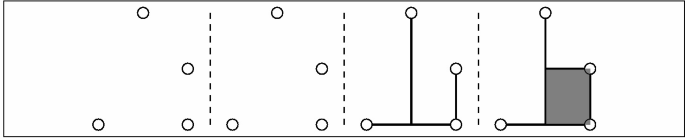
Recursive construction of $\mathcal S ^{\left( i\right) }$. For $i\in \{1,2,\dots \}$, let $\mathcal S ^{\left( i\right) } \subseteq \mathbb {R}^2\times \mathbb {R}^5$ be the set defined recursively from $\mathcal S ^{\left( i-1\right) }$ according to Fig. 1.

Fig. 1.

Recursive procedure to construct $\mathcal S ^{\left( i\right) }$ from $\mathcal S ^{\left( i-1\right) }$ for $i\in \{1,2,\dots \}$.

Fig. 2.

An example showing that the sequence $\{\mathcal S ^{\left( i\right) } \}_{i=0}^\infty$ does not stabilize.

In addition to Theorem 3, we shall also prove the following result.

Theorem 4

(Does not Stabilize). For all $i \in \{1,2, \dotsc \}$, $\mathcal S ^{\left( i-1\right) } \subsetneq \mathcal S ^{\left( i\right) }.$

Intuitively, the choice of the $\mathcal S ^{\left( 0\right) }$ ensures that the evolution of the sets $\mathcal S ^{\left( 0\right) } \rightarrow \mathcal S ^{\left( 1\right) } \rightarrow \mathcal S ^{\left( 2\right) } \rightarrow \cdots$ does not stabilize.

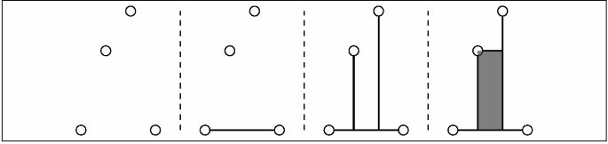
Additional points and notations. We define the following additional points for our analysis (refer to Fig. 2).

$$ a_6 = (1/2, 1/2), \; a_7 = (1/2, 3/4), \; a_8 = (3/4, 3/4)$$

Let $\overline{a_1a_8}$ denote the set of points on the line segment that connects the point $a_1$ to the point $a_8$. The segments $\overline{a_2a_5}, \overline{a_3a_6}, \overline{a_4a_7}$ are defined similarly. For any set $\varOmega \subseteq \mathbb {R}^2$, we define the set $\mathcal S ^{\left( i\right) } _{\varOmega }$ as follows.

$$\mathcal S ^{\left( i\right) } _{\varOmega }\;:=\; \{Q\in \mathcal S ^{\left( i\right) }: \pi (Q)\in \varOmega \}$$

Whenever $\varOmega$ is a singleton set, we omit the brackets. For example,

$$\begin{aligned} \mathcal S _{a_1}^{\left( 0\right) } &=\{(3/4,1/4,1,0,0,0,0)\}, \quad \mathcal S _{a_2}^{\left( 0\right) } =\{(1/4,1/2,0,1,0,0,0)\},\\ \mathcal S _{a_3}^{\left( 0\right) } &=\{(1/2,\; \;\; \; 1,0,0,1,0,0)\},\quad \mathcal S _{a_4}^{\left( 0\right) } =\{(1,3/4,0,0,0,1,0)\},\\ \mathcal S _{a_5}^{\left( 0\right) } &=\{(3/4,1/2,0,0,0,0,1)\},\quad \mathcal S _{a_6}^{\left( 0\right) } =\mathcal S _{a_7}^{\left( 0\right) } =\mathcal S _{a_8}^{\left( 0\right) } =\emptyset . \end{aligned}$$

Moreover, for any set $\varOmega \subseteq \mathbb {R}^2\times \mathbb {R}^5$, we define $\rho \left( \varOmega \right) \;:=\; \{\rho (P): P\in \varOmega \}.$ For example, $\rho (\mathcal S _{a_4}^{\left( 0\right) })=\{(0,0,0,1,0)\}=\{e_4\}$.

For $i \in \{0,1,2,\dots \}$, we define

$$\begin{aligned} &\sigma _i \;:=\; \sum _{k = 0}^{i-1} \frac{1}{16^{k}} = \frac{ 1 - (1/16)^{i}}{1-1/16}, \\&\alpha _i \;:=\;\ \ \ \sigma _{i} \cdot \frac{e_1}{2} + \ \ \ \sigma _{i} \cdot \frac{e_4}{4} + \ \ \ \sigma _{i} \cdot \frac{e_3}{8} + \sigma _{i} \cdot \frac{e_2}{16} + \frac{e_5}{16^i},\\ &\beta _{i} \;:=\; \sigma _{i+1} \cdot \frac{e_2}{2} + \ \ \ \sigma _{i} \cdot \frac{e_1}{4} + \ \ \ \sigma _{i} \cdot \frac{e_4}{8} + \sigma _{i} \cdot \frac{e_3}{16} + \frac{e_5}{2^{4i+1}}, \\ &\gamma _{i} \;:=\; \sigma _{i+1} \cdot \frac{e_3}{2} + \sigma _{i+1} \cdot \frac{e_2}{4} + \ \ \ \sigma _{i} \cdot \frac{e_1}{8} + \sigma _{i} \cdot \frac{e_4}{16} + \frac{e_5}{2^{4i+2}}, \\ &\delta _{i} \;:=\; \sigma _{i+1} \cdot \frac{e_4}{2} + \sigma _{i+1} \cdot \frac{e_3}{4} + \sigma _{i+1} \cdot \frac{e_2}{8} + \sigma _{i} \cdot \frac{e_1}{16} + \frac{e_5}{2^{4i+3}}. \end{aligned}$$

Moreover, $\alpha ^*, \beta ^*, \gamma ^*, \delta ^*$ are defined as the limit of sequences $\alpha _i,\beta _i,\gamma _i,\delta _i$ respectively (refer to Proposition 4). We prove some algebraic properties of $\alpha _i,\beta _i,\gamma _i,\delta _i$ in Sect. 7.4.

Now, we state all claims needed for the proof of Theorem 3. Assuming these claims, we first prove Theorem 3 in Sect. 7.1. Then, we prove these claims in Sect. 7.2

Lemma 2

For every $i \in \{0,1,2,\dots \}$, the following identities hold.

$$\begin{aligned} \rho (\mathcal S _{a_5}^{\left( 4i\right) }) = \rho (\mathcal S _{a_5} ^{\left( 4i+1\right) }) = \rho (\mathcal S _{a_5} ^{\left( 4i+2\right) }) = \rho (\mathcal S _{a_5} ^{\left( 4i+3\right) }), \\ \rho (\mathcal S _{a_6}^{\left( 4i+1\right) }) = \rho (\mathcal S _{a_6} ^{\left( 4i+2\right) }) = \rho (\mathcal S _{a_6} ^{\left( 4i+3\right) }) = \rho (\mathcal S _{a_6} ^{\left( 4i+4\right) }), \\ \rho (\mathcal S _{a_7}^{\left( 4i+2\right) }) = \rho (\mathcal S _{a_7} ^{\left( 4i+3\right) }) = \rho (\mathcal S _{a_7} ^{\left( 4i+4\right) }) = \rho (\mathcal S _{a_5} ^{\left( 4i+5\right) }), \\ \rho (\mathcal S _{a_8}^{\left( 4i+3\right) }) = \rho (\mathcal S _{a_8} ^{\left( 4i+4\right) }) = \rho (\mathcal S _{a_8} ^{\left( 4i+5\right) }) = \rho (\mathcal S _{a_8} ^{\left( 4i+6\right) }). \end{aligned}$$

Lemma 3

For all $i \in \{0,1. \dotsc \}$,

$$\begin{aligned} \rho (\mathcal S _{a_5} ^{\left( 4i\right) }) = \textsf{conv} (\{\alpha _0, \alpha _i)\}), \; \rho (\mathcal S _{a_6} ^{\left( 4i+1\right) }) = \textsf{conv} (\{\beta _0, \beta _i\}), \\ \rho (\mathcal S _{a_7} ^{\left( 4i+2\right) }) = \textsf{conv} (\{\gamma _0, \gamma _i\}), \; \rho (\mathcal S _{a_8} ^{\left( 4i+3\right) }) = \textsf{conv} (\{\delta _0, \delta _i\}). \end{aligned}$$

Lemma 4

For any $i \in \{0,1,2,\dots \}$, it holds that

$$\alpha _{i+1} \notin \rho (\mathcal S _{a_5} ^{\left( 4i\right) }), \; \beta _{i+1} \notin \rho (\mathcal S _{a_6} ^{\left( 4i+1\right) }), \; \gamma _{i+1} \notin \rho (\mathcal S _{a_7} ^{\left( 4i+2\right) }), \; \delta _{i+1} \notin \rho (\mathcal S _{a_8} ^{\left( 4i+3\right) }).$$

7.1 Proofs of Theorem 3 and Theorem 4

Proof

(of Theorem 3). Suppose $r=4k+1$, where $k\in \{0,1,2,\dots \}$. Recall the functionality $f_{4k+1}$ defined in Sect. 5.1

$$\begin{aligned} &f_{4k+1}(0,0)=\left( \frac{3}{16}\cdot \sigma _k, \frac{1}{4}\cdot \sigma _{k+1}, \frac{1}{8}\cdot \sigma _k,\frac{3}{8}\cdot \sigma _k, \frac{3}{2^{4k+2}}\right) \\ &f_{4k+1}(0,1)=\left( \frac{9}{16}\cdot \sigma _k,\frac{1}{4} \cdot \sigma _{k+1}, 0\cdot \sigma _k,\frac{1}{8}\cdot \sigma _k, \frac{3}{2^{4k+2}}\right) \\ &f_{4k+1}(1,0)=\left( \frac{1}{16}\cdot \sigma _k, \frac{3}{4}\cdot \sigma _{k+1},\frac{1}{8}\cdot \sigma _k,0\cdot \sigma _k, \frac{1}{2^{4k+2}}\right) \\ &f_{4k+1}(1,1)=\left( \frac{3}{16}\cdot \sigma _k, \frac{3}{4}\cdot \sigma _{k+1}, 0\cdot \sigma _k,0\cdot \sigma _k, \frac{1}{2^{4k+2}}\right) \\ \end{aligned}$$

where $\sigma _k \;:=\; \frac{1 - (1/16)^k}{1 - 1/16}$ for $k \in \{0,1,2,\dotsc \}$. As we discussed in Sect. 5.1, the encoding of $f_{4k+1}$ is the triplet $(A, B, V_{4k+1})$, where

$$\begin{aligned} &A = \begin{pmatrix} 3/4,&{}\; 1/4, &{}\; 1/2, &{}\; 1, &{}\; 3/4\\ 1/4,&{}\; 3/4, &{}\; 1/2, &{}\; 0, &{}\; 1/4 \end{pmatrix} \in \mathcal M _{2\times 5}(\mathbb {R}), \\ &B= \begin{pmatrix} 1/4, &{}\; 1/2, &{}\; 1, &{}\; 3/4, &{}\; 1/2\\ 3/4, &{}\; 1/2, &{}\; 0, &{}\; 1/4, &{}\; 1/2 \end{pmatrix} \in \mathcal M _{2\times 5}(\mathbb {R}), \\ &V_{4k+1} = \left( \sigma _k, 2\sigma _{k+1}, \frac{\sigma _k}{4}, \frac{\sigma _k}{2}, \frac{1}{2^{4k-1}}\right) \in \mathbb {R}^5. \end{aligned}$$

and the query point is the following:

$$Q(f_{4k+1}) = \left( \frac{1}{2},\; \frac{1}{2},\; \frac{1}{4}\cdot \frac{\sigma _k}{4},\; \frac{\sigma _{k+1}}{2},\; \frac{\sigma _k}{16},\; \frac{\sigma _k}{8},\; \frac{1}{2^{4k+1}} \right) \in \mathbb {R}^7.$$

Now, recall that

$$ \beta _{k}= \sigma _{k+1} \cdot \frac{e_2}{2} + \ \ \ \sigma _{k} \cdot \frac{e_1}{4} + \ \ \ \sigma _{k} \cdot \frac{e_4}{8} + \sigma _{k} \cdot \frac{e_3}{16} + \frac{e_5}{2^{4k+1}}$$

This implies $\rho \left( Q(f_{4k+1})\right) =\beta _k$. Thus, it follows from Lemma 3 and Lemma 4 that $\rho (Q(f_{4k+1}))\in \mathcal S _{a_6}^{\left( 4k+1\right) }$ but $\rho (Q(f_{4k+1}))\not \in \mathcal S _{a_6}^{\left( 4(k-1)+1\right) }$. Moreover, Lemma 2 implies that $\mathcal S _{a_6}^{\left( 4(k-1)+1\right) } =\mathcal S _{a_6}^{\left( 4k\right) }$. Thus, we conclude that

$$Q(f_{4k+1}) \in \mathcal S ^{\left( 4k+1\right) } \setminus \mathcal S ^{\left( 4k\right) } $$

which is what we promised to prove in Lemma 1. This implies that $f_r$ has r round secure protocol but no $(r-1)$ secure protocol.

We can extend the proof to the case that $r\not =4k+1$ for any k. The idea is similar. We can find 3 different family of functions corresponding to $r=4k, r=4k+2, r=4k+3$. We only need to choose a different query point in Fig. 2, $a_5, a_7$, or $a_8$ and scale that figure and transfer it appropriately such that query points (1/2, 1/2) is on $a_5, a_7$, or $a_8$ depending on the remainder of division of r by 4. Then, we can find appropriate functionalities. This completes the proof of the theorem.

Proof

(of Theorem 4). Theorem 4 follows directly from Lemma 3 and Lemma 2.

7.2 Proofs of Claims Needed for Theorem 3

This section proves all the claims needed for Theorem 3 assuming other results that will be proved in Sect. 7.3.

Proof

(of Lemma 2). We prove by induction on i.

Base Case. From the recursion in Lemma 6, one can verify that

$$\begin{aligned} &\rho (\mathcal S _{a_5} ^{\left( 0\right) }) = \rho (\mathcal S _{a_5} ^{\left( 1\right) }) = \rho (\mathcal S _{a_5} ^{\left( 2\right) }) = \rho (\mathcal S _{a_5} ^{\left( 3\right) }) = \{e_5\}, \\ &\rho (\mathcal S _{a_6} ^{\left( 1\right) }) = \rho (\mathcal S _{a_6} ^{\left( 2\right) }) = \rho (\mathcal S _{a_6} ^{\left( 3\right) }) = \rho (\mathcal S _{a_6} ^{\left( 4\right) }) = \frac{e_2 + e_5}{2}, \\ &\rho (\mathcal S _{a_7} ^{\left( 2\right) }) = \rho (\mathcal S _{a_7} ^{\left( 3\right) }) = \rho (\mathcal S _{a_7} ^{\left( 4\right) }) = \rho (\mathcal S _{a_7} ^{\left( 5\right) }) = \frac{e_3}{2} + \frac{e_2 + e_5}{4}, \\ &\rho (\mathcal S _{a_8} ^{\left( 3\right) }) = \rho (\mathcal S _{a_8} ^{\left( 4\right) }) = \rho (\mathcal S _{a_8} ^{\left( 5\right) }) = \rho (\mathcal S _{a_8} ^{\left( 6\right) }) = \frac{e_4}{2} + \frac{e_3}{4} + \frac{e_2 + e_5}{8}. \end{aligned}$$

Induction Step. Suppose the induction hypothesis holds for $(i-1)$. It follows from Lemma 6 that

$$\begin{aligned} \rho (\mathcal S _{a_5} ^{\left( 4i+3\right) }) &= \textsf{conv} \left( \rho (\mathcal S _{a_5} ^{\left( 4i+2\right) }) \cup \frac{1}{2}\cdot \left( e_1 + \rho (\mathcal S _{a_8} ^{\left( 4i+2\right) })\right) \right) \end{aligned}$$

$$\begin{aligned} &= \textsf{conv} \left( \textsf{conv} \left( \rho (\mathcal S _{a_5} ^{\left( 4i+1\right) }) \cup \frac{1}{2}\cdot \left( e_1 + \rho (\mathcal S _{a_8} ^{\left( 4i+1\right) })\right) \right) \cup \frac{1}{2}\cdot \left( e_1 + \rho (\mathcal S _{a_8} ^{\left( 4i+2\right) })\right) \right) \end{aligned}$$

By the induction hypothesis, $\rho (\mathcal S _{a_8} ^{\left( 4i+2\right) }) = \rho (\mathcal S _{a_8} ^{\left( 4i+1\right) })$. Therefore, we have

$$\begin{aligned} \frac{1}{2}\cdot \left( e_1 + \rho (\mathcal S _{a_8} ^{\left( 4i+1\right) })\right) = \frac{1}{2}\cdot \left( e_1 + \rho (\mathcal S _{a_8} ^{\left( 4i+2\right) })\right) \end{aligned}$$

This, together with Fact 1 and Lemma 6, implies that

$$\begin{aligned} \rho (\mathcal S _{a_5} ^{\left( 4i+3\right) }) = \textsf{conv} \left( \rho (\mathcal S _{a_5} ^{\left( 4i+1\right) }) \cup \frac{1}{2}\cdot \left( e_1 + \rho (\mathcal S _{a_8} ^{\left( 4i+1\right) })\right) \right) = \rho (\mathcal S _{a_5} ^{\left( 4i+2\right) }). \end{aligned}$$

Likewise, one can show that $\rho (\mathcal S _{a_5} ^{\left( 4i+2\right) }) = \rho (\mathcal S _{a_5} ^{\left( 4i+1\right) })$ and $\rho (\mathcal S _{a_5} ^{\left( 4i+1\right) }) = \rho (\mathcal S _{a_5} ^{\left( 4i\right) })$. These imply that

$$\rho (\mathcal S _{a_5}^{\left( 4i\right) }) = \rho (\mathcal S _{a_5} ^{\left( 4i+1\right) }) = \rho (\mathcal S _{a_5} ^{\left( 4i+2\right) }) = \rho (\mathcal S _{a_5} ^{\left( 4i+3\right) }).$$

The proof of other equalities is similar.

Proof

(of Lemma 3). We prove by induction on i (refer to Fig. 3).

Fig. 3.

The evolution of $\rho (\mathcal S ^{\left( i\right) } _{a_5}),\rho (\mathcal S ^{\left( i\right) } _{a_6}),\rho (\mathcal S ^{\left( i\right) } _{a_7}),\rho (\mathcal S ^{\left( i\right) } _{a_8})$ up to step eight.

Base Case. For $i = 0$,

$$\begin{aligned} &\rho (\mathcal S _{a_5} ^{\left( 0\right) }) = \{ \alpha _0 \} = \{e_5 \}, \\ &\rho (\mathcal S _{a_6} ^{\left( 1\right) }) = \{ \beta _0 \}= \left\{ \frac{e_2 + e_5}{2}\right\} , \\ &\rho (\mathcal S _{a_7} ^{\left( 2\right) }) = \{ \gamma _0 \} = \left\{ \frac{e_3}{2} + \frac{e_2+e_5}{4}\right\} , \\ &\rho (\mathcal S _{a_8} ^{\left( 3\right) }) = \{ \delta _0 \}= \left\{ \frac{e_4}{2} + \frac{e_3}{4} + \frac{e_2+e_5}{8}\right\} . \end{aligned}$$

Induction Step. Suppose the lemma is true for i. We shall show that it is true for $i+1$.

$$\begin{aligned} \rho (\mathcal S _{a_5} ^{\left( 4i+4)\right) }) &= \textsf{conv} \left( \rho (\mathcal S _{a_5} ^{\left( 4i+3\right) }) \cup \frac{1}{2} \left( e_1 + \rho (\mathcal S _{a_8} ^{\left( 4i+3\right) })\right) \right) & (Lemma~6) \\ & = \textsf{conv} \left( \rho (\mathcal S _{a_5} ^{\left( 4i\right) }) \cup \frac{1}{2} \left( e_1 + \rho (\mathcal S _{a_8} ^{\left( 4i+3\right) })\right) \right) & (Lemma~2) \\ & = \textsf{conv} \left( \textsf{conv} (\{\alpha _0, \alpha _i \}) \cup \frac{1}{2} \left( e_1 + \textsf{conv} (\{\delta _0, \delta _i \})\right) \right) & (\text {Induction hypothesis}) \\ & = \textsf{conv} \left( \{\alpha _0, \alpha _i \} \cup \left\{ \frac{e_1+\delta _0}{2}, \frac{e_1+\delta _i}{2}\right\} \right) & (Fact ~1) \\ & = \textsf{conv} \left( \{\alpha _0, \alpha _i \} \cup \{\alpha _1, \alpha _{i+1}\} \right) & Proposition\,2 \\ &= \textsf{conv} (\{ \alpha _0, \alpha _{i+1} \}) & (Proposition\,5 \text { and } Fact~2) \end{aligned}$$

Similarly, it holds that

$$\begin{aligned} \rho (\mathcal S _{a_6} ^{\left( 4i+5\right) }) = \textsf{conv} (\{\beta _0, \beta _{i+1}\}), \\ \rho (\mathcal S _{a_7} ^{\left( 4i+6)\right) } = \textsf{conv} (\{\gamma _0, \gamma _{i+1}\}), \\ \rho (\mathcal S _{a_8} ^{\left( 4i+7\right) }) = \textsf{conv} (\{\delta _0, \delta _{i+1}\}), \end{aligned}$$

which completes the proof.

Proof

(of Lemma 4). Lemma 4 follows directly from Lemma 3 and Proposition 5.

7.3 Proof of Claims Needed for Lemma 2, Lemma 3, and Lemma 4

This section proves results that are needed for the proof of Lemma 2, Lemma 3, and Lemma 4. The result below follows directly from the definition of the sequence $\{\mathcal S _i\}_{i=0}^\infty$.

Proposition 1

For any set $\varOmega$ and any $i \in \{0,1, \dotsc \}$, the following property holds.

$$\mathcal S _\varOmega ^{\left( i\right) } \subseteq \mathcal S _\varOmega ^{\left( i+1\right) }.$$

The following result says that for any $i \in \{0,1,\dotsc \}$, all the points in the line segment $\overline{a_1a_8}$ at round $(i+1)$ except the new ones at the point $a_8$ are constructed solely from the points at $a_1, a_8, a_5$ at round i, and similarly for others.

Lemma 5

For every $i \in \{0,1,\dotsc \}$,

$$\mathcal S _{\overline{a_1a_8}}^{\left( i+1\right) } \setminus \left( \mathcal S _{a_8} ^{\left( i+1\right) } \setminus \mathcal S _{a_8} ^{\left( i\right) } \right) = \textsf{conv} \left( \mathcal S _{a_1}^{\left( i\right) } \cup \mathcal S _{a_8} ^{\left( i\right) } \cup \mathcal S _{a_5} ^{\left( i\right) } \right) ,$$

$$\mathcal S _{\overline{a_2a_5}}^{\left( i+1\right) } \setminus \left( \mathcal S _{a_5}^{\left( i+1\right) } \setminus \mathcal S _{a_5}^{\left( i\right) } \right) = \textsf{conv} \left( \mathcal S _{a_2}^{\left( i\right) } \cup \mathcal S _{a_5} ^{\left( i\right) } \cup \mathcal S _{a_6} ^{\left( i\right) } \right) ,$$

$$\mathcal S _{\overline{a_3a_6}}^{\left( i+1\right) } \setminus \left( \mathcal S _{a_6}^{\left( i+1\right) } \setminus \mathcal S _{a_6}^{\left( i\right) } \right) = \textsf{conv} \left( \mathcal S _{a_3}^{\left( i\right) } \cup \mathcal S _{a_6} ^{\left( i\right) } \cup \mathcal S _{a_7} ^{\left( i\right) } \right) ,$$

$$\mathcal S _{\overline{a_4a_7}}^{\left( i+1\right) } \setminus \left( \mathcal S _{a_7}^{\left( i+1\right) } \setminus \mathcal S _{a_7}^{\left( i\right) } \right) = \textsf{conv} \left( \mathcal S _{a_4}^{\left( i\right) } \cup \mathcal S _{a_7} ^{\left( i\right) } \cup \mathcal S _{a_8} ^{\left( i\right) } \right) .$$

Proof

(of Lemma 5). We prove by induction on i.

Base Case. For $i=0$, we have

$$\mathcal S _{a_1} ^{\left( 0\right) } = \{(3/4, 1/4, 1, 0, 0, 0, 0, 0)\}, \; \mathcal S _{a_5} ^{\left( 0\right) } = \{(3/4, 1/2, 0, 0 , 0, 0, 1)\}, \; \mathcal S _{a_8} ^{\left( 0\right) } = \emptyset .$$

It implies that

$$ \textsf{conv} \left( \mathcal S _{a_1}^{\left( 0\right) } \cup \mathcal S _{a_8} ^{\left( 0\right) } \cup \mathcal S _{a_5} ^{\left( 0\right) } \right) = \textsf{conv} \left( \mathcal S _{a_1}^{\left( 0\right) } \cup \mathcal S _{a_5} ^{\left( 0\right) } \right) .$$

Observe that $\pi _1(P)=3/4$, for any point $P\in \mathcal S _{a_1} ^{\left( 0\right) } \cup \mathcal S _{a_5} ^{\left( 0\right) }$. Therefore, any convex combination of a point in $\mathcal S _{a_1} ^{\left( 0\right) }$ and a point in $\mathcal S _{a_5} ^{\left( 0\right) }$ is in the set $\mathcal S _{\overline{a_1a_8}} ^{\left( 1\right) }$. Notice that $\mathcal S _{a_8}^{\left( 0\right) } =\mathcal S _{a_8}^{\left( 1\right) } =\emptyset$. This shows that

$$\textsf{conv} \left( \mathcal S _{a_1}^{\left( 0\right) } \cup \mathcal S _{a_8} ^{\left( 0\right) } \cup \mathcal S _{a_5} ^{\left( 0\right) } \right) \subseteq \mathcal S _{\overline{a_1a_8}} ^{\left( 1\right) } =\mathcal S _{\overline{a_1a_8}} ^{\left( 1\right) } \setminus \left( \mathcal S _{a_8} ^{\left( 1\right) } \setminus \mathcal S _{a_8}^{\left( 0\right) } \right) .$$

To prove the other direction, observe that any point in $\mathcal S _{\overline{a_1a_8}} ^{\left( 1\right) }$ except for the points in $\mathcal S _{a_8} ^{\left( 1\right) } \setminus \mathcal S _{a_8} ^{\left( 0\right) }$ is a convex combination of a set of points in $\mathcal S _{\overline{a_1a_8}} ^{\left( 0\right) } = \mathcal S _{a_1} ^{\left( 0\right) } \cup \mathcal S _{a_5} ^{\left( 0\right) }$ by definition. Thus, it follows that

$$\mathcal S _{\overline{a_1a_8}} ^{\left( 1\right) } \setminus \left( \mathcal S _{a_8} ^{\left( 1\right) } \setminus \mathcal S _{a_8}^{\left( 0\right) } \right) =\mathcal S _{\overline{a_1a_8}} ^{\left( 1\right) } \subseteq \textsf{conv}\!\left( {\mathcal S _{a_1} ^{\left( 0\right) }} \cup {\mathcal S _{a_5} ^{\left( 0\right) }}\right) =\textsf{conv} \left( \mathcal S _{a_1}^{\left( 0\right) } \cup \mathcal S _{a_8} ^{\left( 0\right) } \cup \mathcal S _{a_5} ^{\left( 0\right) } \right) .$$

Induction Hypothesis. We assume that

$$\mathcal S _{\overline{a_1a_8}}^{\left( i\right) } \setminus \left( \mathcal S _{a_8} ^{\left( i\right) } \setminus \mathcal S _{a_8} ^{\left( i-1\right) } \right) = \textsf{conv} \left( \mathcal S _{a_1}^{\left( i-1\right) } \cup \mathcal S _{a_8} ^{\left( i-1\right) } \cup \mathcal S _{a_5} ^{\left( i-1\right) } \right) ,$$

and similarly for other equations.

Induction Step. Note that for any point P in the set $\mathcal S _{a_1}^{\left( i\right) } \cup \mathcal S _{a_8}^{\left( i\right) } \cup \mathcal S _{a_5}^{\left( i\right) }$, we have $\pi _1(P)=3/4$. Therefore,

$$\textsf{conv} \left( \mathcal S _{a_1}^{\left( i\right) } \cup \mathcal S _{a_8}^{\left( i\right) } \cup \mathcal S _{a_5}^{\left( i\right) } \right) \subseteq \mathcal S _{\overline{a_1a_8}} ^{\left( i+1\right) } $$

Since $\overline{a_4a_7}$ is the only line segment that contains $a_8$ such that $a_8$ is not an end point of it, we have:

$$\begin{aligned} \left( \mathcal S _{a_8}^{\left( i+1\right) } \setminus \mathcal S _{a_8}^{\left( i\right) } \right) \cap \textsf{conv} \left( \mathcal S _{a_1}^{\left( i\right) } \cup \mathcal S _{a_8}^{\left( i\right) } \cup \mathcal S _{a_5}^{\left( i\right) } \right) &=\left( \mathcal S _{a_8}^{\left( i+1\right) } \setminus \mathcal S _{a_8}^{\left( i\right) } \right) \cap \textsf{conv} \left( \mathcal S _{a_8}^{\left( i\right) } \right) =\emptyset . \end{aligned}$$

Therefore, we conclude that

$$\textsf{conv} \left( \mathcal S _{a_1}^{\left( i\right) } \cup \mathcal S _{a_8}^{\left( i\right) } \cup \mathcal S _{a_5}^{\left( i\right) } \right) \subseteq \mathcal S _{\overline{a_1a_8}} ^{\left( i+1\right) } \setminus \left( \mathcal S _{a_8}^{\left( i+1\right) } \setminus \mathcal S _{a_8}^{\left( i\right) } \right) .$$

To prove the other direction, note that any point in $\mathcal S _{\overline{a_1a_8}} ^{\left( i+1\right) } \setminus \mathcal S _{a_8} ^{\left( i+1\right) }$ is constructed from a convex combination of the points in $\mathcal S _{\overline{a_1a_8}} ^{\left( i\right) } \setminus \mathcal S _{a_8} ^{\left( i\right) }$. Thus, we have

$$\begin{aligned} \mathcal S _{\overline{a_1a_8}} ^{\left( i+1\right) } \setminus \mathcal S _{a_8} ^{\left( i+1\right) } &\subseteq \textsf{conv} \left( \mathcal S _{\overline{a_1a_8}} ^{\left( i\right) } \setminus \mathcal S _{a_8} ^{\left( i\right) } \right) \\ &\subseteq \textsf{conv} \left( \mathcal S _{\overline{a_1a_8}} ^{\left( i\right) } \setminus \left( \mathcal S _{a_8} ^{\left( i\right) } \setminus \mathcal S _{a_8} ^{\left( i-1\right) } \right) \right) & (Fact~2)\\ &=\textsf{conv} \left( \textsf{conv} \left( \mathcal S _{a_1}^{\left( i-1\right) } \cup \mathcal S _{a_8} ^{\left( i-1\right) } \cup \mathcal S _{a_5} ^{\left( i-1\right) } \right) \right) & (\text {Induction hypothesis})\\ &= \textsf{conv} \left( \mathcal S _{a_1}^{\left( i-1\right) } \cup \mathcal S _{a_8} ^{\left( i-1\right) } \cup \mathcal S _{a_5} ^{\left( i-1\right) } \right) & (Fact~1)\\ & \subseteq \textsf{conv} \left( \mathcal S _{a_1}^{\left( i\right) } \cup \mathcal S _{a_8} ^{\left( i\right) } \cup \mathcal S _{a_5} ^{\left( i\right) } \right) , & (Proposition\,1 \text { and } Fact~2) \end{aligned}$$

Since $\mathcal S _{a_8} ^{\left( i\right) } \subseteq \textsf{conv} \left( \mathcal S _{a_1}^{\left( i\right) } \cup \mathcal S _{a_8} ^{\left( i\right) } \cup \mathcal S _{a_5} ^{\left( i\right) } \right)$, it follows that

$$\begin{aligned} \mathcal S _{\overline{a_1a_8}}^{\left( i+1\right) } \setminus \left( \mathcal S _{a_8} ^{\left( i+1\right) } \setminus \mathcal S _{a_8} ^{\left( i\right) } \right) = \left( \mathcal S _{\overline{a_1a_8}} ^{\left( i+1\right) } \setminus \mathcal S _{a_8} ^{\left( i+1\right) } \right) \cup \mathcal S _{a_8} ^{\left( i\right) } \subseteq \textsf{conv} \left( \mathcal S _{a_1}^{\left( i\right) } \cup \mathcal S _{a_8} ^{\left( i\right) } \cup \mathcal S _{a_5} ^{\left( i\right) } \right) . \end{aligned}$$

We have shown that

$$\begin{aligned} \mathcal S _{\overline{a_1a_8}}^{\left( i+1\right) } \setminus \left( \mathcal S _{a_8} ^{\left( i+1\right) } \setminus \mathcal S _{a_8} ^{\left( i\right) } \right) = \textsf{conv} \left( \mathcal S _{a_1}^{\left( i\right) } \cup \mathcal S _{a_8} ^{\left( i\right) } \cup \mathcal S _{a_5} ^{\left( i\right) } \right) . \end{aligned}$$

We prove other equations in a similar manner, which completes the proof.

Next, using Lemma 5, we prove a recursive construction of the projection $\rho$ at the points $a_i$ for $1\leqslant i \leqslant 8$.

Lemma 6

For all $i \in \{0,1, \dotsc \}$,

$$\begin{aligned} \rho (\mathcal S _{a_1}^{\left( i\right) })=\{e_1\}, \; \rho (\mathcal S _{a_2}^{\left( i\right) })=\{e_2\}, \; \rho (\mathcal S _{a_3}^{\left( i\right) })=\{e_3\}, \; \rho (\mathcal S _{a_4}^{\left( i\right) })=\{e_4\}. \end{aligned}$$

Furthermore, for all $i \in \{1,2, \dotsc , \}$,

$$\begin{aligned} \rho (\mathcal S _{a_5} ^{\left( 0\right) }) = \{e_5\}, \; \rho (\mathcal S _{a_5} ^{\left( i+1\right) }) = \textsf{conv}\!\left( {\rho (\mathcal S _{a_5}^{\left( i\right) })} \cup {\frac{1}{2}\cdot \left( e_1 + \rho (\mathcal S _{a_8} ^{\left( i\right) })\right) }\right) , \\ \rho (\mathcal S _{a_6}^{\left( 0\right) }) =\emptyset , \; \rho (\mathcal S _{a_6} ^{\left( i+1\right) }) = \textsf{conv}\!\left( {\rho (\mathcal S _{a_6}^{\left( i\right) })} \cup {\frac{1}{2}\cdot \left( e_2 + \rho (\mathcal S _{a_5} ^{\left( i\right) })\right) }\right) , \\ \rho (\mathcal S _{a_7}^{\left( 0\right) }) = \emptyset , \; \rho (\mathcal S _{a_7} ^{\left( i+1\right) }) = \textsf{conv}\!\left( {\rho (\mathcal S _{a_7}^{\left( i\right) })} \cup {\frac{1}{2}\cdot \left( e_3 + \rho (\mathcal S _{a_6} ^{\left( i\right) })\right) }\right) , \\ \rho (\mathcal S _{a_8}^{\left( 0\right) }) = \emptyset , \; \rho (\mathcal S _{a_8} ^{\left( i+1\right) }) = \textsf{conv}\!\left( {\rho (\mathcal S _{a_8}^{\left( i\right) })} \cup {\frac{1}{2}\cdot \left( e_4 + \rho (\mathcal S _{a_7} ^{\left( i\right) })\right) }\right) . \end{aligned}$$

Proof

(of Lemma 6). Initially, $\rho (\mathcal S _{a_1} ^{\left( 0\right) }) = \{e_1 \}$. At any round $i \in \{1,2 \dotsc \}$, there is no new point constructed at $a_1$, since $a_1$ is an extreme point of $\textsf{conv} ( a_1,a_2,a_3,a_4,a_5)$. Therefore, $\rho (\mathcal S _{a_1} ^{\left( i\right) }) = \{e_1 \}$. Similarly, we have

$$\rho (\mathcal S _{a_2}^{\left( i\right) })=\{e_2\}, \; \rho (\mathcal S _{a_3}^{\left( i\right) })=\{e_3\}, \; \rho (\mathcal S _{a_4}^{\left( i\right) })=\{e_4\}, \text { for every } i \in \{0,1, \dotsc \}.$$

Let $P \in \mathcal S _{a_5} ^{\left( i+1\right) }$. It follows from Lemma 5 that there are points $P_{a_1} \in \mathcal S _{a_1} ^{\left( i\right) }$, $P_{a_8} \in \mathcal S _{a_8} ^{\left( i\right) }$, $P_{a_5} \in \mathcal S _{a_5} ^{\left( i\right) }$, and $\lambda _1, \lambda _8, \lambda _5 \geqslant 0$ such that

$$\begin{aligned} P = \lambda _1 \cdot P_{a_1} + \lambda _8 \cdot P_{a_8} + \lambda _5 \cdot P_{a_5}, \; \text{ and } \lambda _1+\lambda _8+\lambda _5=1. \end{aligned}$$

Projecting these points into the second coordinate, we have

$$\pi _2(P) = \lambda _1 \cdot \pi _2(P_{a_1}) + \lambda _8 \cdot \pi _2(P_{a_8}) + \lambda _5 \cdot \pi _2(P_{a_5}).$$

This together with $\pi _2(P) = \pi _2(P_{a_5}) = \frac{1}{2}\left( \pi _2(P_{a_1}) + \pi _2(P_{a_8})\right)$ implies that $\lambda _1 = \lambda _8$. Thus, the point P is in the set $\textsf{conv} \left( \mathcal S _{a_5} ^{\left( i\right) } \cup \frac{1}{2} \cdot \left( \mathcal S _{a_1}^{\left( i\right) } + \mathcal S _{a_8} ^{\left( i\right) } \right) \right)$. This implies that

$$\mathcal S _{a_5} ^{\left( i+1\right) } \subseteq \textsf{conv} \left( \mathcal S _{a_5} ^{\left( i\right) } \cup \frac{1}{2} \cdot \left( \mathcal S _{a_1}^{\left( i\right) } + \mathcal S _{a_8} ^{\left( i\right) } \right) \right) .$$

Projecting this fact into coordinates $\{3,4,5,6,7\}$ yields

$$\begin{aligned} \rho (\mathcal S _{a_5} ^{\left( i+1\right) }) & \subseteq \textsf{conv}\!\left( {\rho (\mathcal S _{a_5}^{\left( i\right) })} \cup {\frac{1}{2}\cdot \left( \rho (\mathcal S _{a_1} ^{\left( i\right) }) \cup \rho (\mathcal S _{a_8} ^{\left( i\right) })\right) }\right) \\ &= \textsf{conv}\!\left( {\rho (\mathcal S _{a_5}^{\left( i\right) })} \cup {\frac{1}{2}\cdot \left( e_1 + \rho (\mathcal S _{a_8} ^{\left( i\right) })\right) }\right) & (\text {since } \rho (\mathcal S _{a_1} ^{\left( i\right) }) = \{e_1\}). \end{aligned}$$

Conversely, it suffices to show that

$$\textsf{conv} \left( \mathcal S _{a_5} ^{\left( i\right) } \cup \frac{1}{2} \cdot \left( \mathcal S _{a_1}^{\left( i\right) } + \mathcal S _{a_8} ^{\left( i\right) } \right) \right) \subseteq \mathcal S _{a_5} ^{\left( i+1\right) }.$$

This follows directly from the fact that $a_5$ is the midpoint of the segment $\overline{a_1a_8}$. We have proved that

$$ \rho (\mathcal S _{a_5} ^{\left( i+1\right) }) = \textsf{conv}\!\left( {\rho (\mathcal S _{a_5}^{\left( i\right) })} \cup {\frac{1}{2}\cdot \left( e_1 + \rho (\mathcal S _{a_8} ^{\left( i\right) })\right) }\right) .$$

Similarly, the other three equations for $a_6, a_7, a_8$ also hold.

7.4 Properties of the Four Sequences

We first recall the definition of the four sequences $\alpha _i, \beta _i, \gamma _i, \sigma _i$ as follows. For $i \in \{0,1,2,\dots \}$,

$$\begin{aligned} &\sigma _i \;:=\; \sum _{k = 0}^{i-1} \frac{1}{16^{k}} = \frac{ 1 - (1/16)^{i}}{1-1/16}, \\&\alpha _i \;:=\;\ \ \ \sigma _{i} \cdot \frac{e_1}{2} + \ \ \ \sigma _{i} \cdot \frac{e_4}{4} + \ \ \ \sigma _{i} \cdot \frac{e_3}{8} + \sigma _{i} \cdot \frac{e_2}{16} + \frac{e_5}{16^i}, \\ &\beta _{i} \;:=\; \sigma _{i+1} \cdot \frac{e_2}{2} + \ \ \ \sigma _{i} \cdot \frac{e_1}{4} + \ \ \ \sigma _{i} \cdot \frac{e_4}{8} + \sigma _{i} \cdot \frac{e_3}{16} + \frac{e_5}{2^{4i+1}}, \\ &\gamma _{i} \;:=\; \sigma _{i+1} \cdot \frac{e_3}{2} + \sigma _{i+1} \cdot \frac{e_2}{4} + \ \ \ \sigma _{i} \cdot \frac{e_1}{8} + \sigma _{i} \cdot \frac{e_4}{16} + \frac{e_5}{2^{4i+2}}, \\ &\delta _{i} \;:=\; \sigma _{i+1} \cdot \frac{e_4}{2} + \sigma _{i+1} \cdot \frac{e_3}{4} + \sigma _{i+1} \cdot \frac{e_2}{8} + \sigma _{i} \cdot \frac{e_1}{16} + \frac{e_5}{2^{4i+3}}. \end{aligned}$$

Proposition 2

For all $i \in \{0,1, \dotsc \}$,

$$\begin{aligned} \alpha _{i+1} = \frac{e_1 + \delta _i}{2}, \; \beta _{i} = \frac{e_2 + \alpha _i}{2}, \; \gamma _{i} = \frac{e_3 + \beta _i}{2}, \; \delta _{i} = \frac{e_4 + \gamma _i}{2}. \end{aligned}$$

Proof

By definition,

$$\begin{aligned} \frac{e_2+\alpha _i}{2} &=\frac{e_2}{2}+\frac{\sigma _i}{2}\cdot (\frac{e_1}{2}+\frac{e_4}{4}+\frac{e_3}{8}+\frac{e_2}{16})+\frac{e_5}{2\cdot 16^i}\\ &=\frac{e_2}{2}+\frac{\sigma _i}{2}\cdot (\frac{e_1}{2}+\frac{e_4}{4}+\frac{e_3}{8}+\frac{e_2}{16})+\frac{e_5}{2\cdot 16^i}\\ &=\left( 1+\frac{\sigma _i}{16}\right) \cdot \frac{e_2}{2}+ \sigma _i\cdot (\frac{e_1}{4}+\frac{e_4}{8}+\frac{e_3}{16})+\frac{e_5}{2\cdot 16^i}\\ &=\sigma _{i+1}\cdot \frac{e_2}{2}+ \sigma _i\cdot (\frac{e_1}{4}+\frac{e_4}{8}+\frac{e_3}{16})+\frac{e_5}{2\cdot 16^i} & (Proposition\,Proposition\,3)\\ &=\beta _i \end{aligned}$$

The proofs of the other equations are similar.

The following proposition follows from the definition of $\sigma _i.$

Proposition 3

For all $i \in \{1,2,\dotsc \}$,

$$\sigma _{i}=1+\frac{1}{16}\sigma _{i-1}.$$

Proposition 4

The following statements hold.

$$\begin{aligned} \lim _{i \rightarrow \infty } \alpha _i = \frac{8}{15} e_1 + \frac{4}{15} e_4 + \frac{2}{15} e_3 + \frac{1}{15} e_2 \;=:\; \alpha ^*, \\ \lim _{i \rightarrow \infty } \beta _i = \frac{8}{15} e_2 + \frac{4}{15} e_1 + \frac{2}{15} e_4 + \frac{1}{15} e_3 \;=:\; \beta ^*, \\ \lim _{i \rightarrow \infty } \gamma _i = \frac{8}{15} e_3 + \frac{4}{15} e_2 + \frac{2}{15} e_1 + \frac{1}{15} e_4 \;=:\; \gamma ^*,\\ \lim _{i \rightarrow \infty } \delta _i = \frac{8}{15} e_4 + \frac{4}{15} e_3 + \frac{2}{15} e_2 + \frac{1}{15} e_1 \;=:\; \delta ^*. \end{aligned}$$

Proof

First, note that

$$\lim _{i\rightarrow \infty }\sigma _{i-1}=\lim _{i\rightarrow \infty }\sigma _{i}=\lim _{i\rightarrow \infty }\frac{1-(1/16)^i}{1-1/16}=16/15.$$

Now, we have

$$\begin{aligned} \lim _{i\rightarrow \infty } \alpha _i &=\lim _{i\rightarrow \infty } \sigma _{i}\cdot \left( \frac{e_1}{2}+\frac{e_4}{4}+\frac{e_3}{8}+\frac{e_2}{16}\right) +\frac{e_5}{16^i}\\ &=\frac{16}{15}\cdot \left( \frac{e_1}{2}+\frac{e_4}{4}+\frac{e_3}{8}+\frac{e_2}{16}\right) \\ &=\frac{8}{15} e_1 + \frac{4}{15} e_4 + \frac{2}{15} e_3 + \frac{1}{15} e_2=\alpha ^*. \end{aligned}$$

Similarly, we can find the $\lim _{i\rightarrow \infty } \beta _i=\beta ^*, \lim _{i\rightarrow \infty } \gamma _i=\gamma ^*$, and $\lim _{i\rightarrow \infty } \delta _i=\delta ^*$ (Fig. 4).

Fig. 4.

Visualization of sequence $\{\beta _i\}_{i=1}^{\infty }$ (refer to Proposition 5)

Proposition 5

For all $i \in \{0,1,\dotsc \}$,

$$\begin{aligned} &\alpha _{i+1} = \frac{15}{16} \cdot \alpha ^* + \frac{1}{16} \cdot \alpha _i, \quad \beta _{i+1} = \frac{15}{16} \cdot \beta ^* + \frac{1}{16} \cdot \beta _i, \\ &\gamma _{i+1} = \frac{15}{16} \cdot \gamma ^* + \frac{1}{16} \cdot \gamma _i, \; \quad \delta _{i+1} = \frac{15}{16} \cdot \delta ^* + \frac{1}{16} \cdot \delta _i. \end{aligned}$$

Consequently, $\alpha _i$ is on the line segment between $\alpha _0=e_5$ and $\alpha _{i+1}$; and $\alpha _{i+1}$ is on the line segment between $\alpha _i$ and $\alpha ^*$. More formally,

$$\begin{aligned} &\alpha _i \in \textsf{conv} (\alpha _0, \alpha _{i+1}), \; \alpha _{i+1} \in \textsf{conv} (\alpha _{i}, \alpha ^*), \\ &\beta _i \in \textsf{conv} (\beta _0, \beta _{i+1}), \; \beta _{i+1} \in \textsf{conv} (\beta _{i}, \beta ^*), \\ &\gamma _i \in \textsf{conv} (\gamma _0, \gamma _{i+1}), \; \gamma _{i+1} \in \textsf{conv} (\gamma _{i}, \gamma ^*), \\ &\delta _i \in \textsf{conv} (\delta _0, \delta _{i+1}), \; \delta _{i+1} \in \textsf{conv} (\delta _{i}, \delta ^*). \\ \end{aligned}$$

Proof

By definition,

$$\alpha _{i}=\sigma _{i}\cdot \left( \frac{e_1}{2}+\frac{e_4}{4}+\frac{e_3}{8}+\frac{e_2}{16}\right) +\frac{e_5}{16^{i}}.$$

So, we have

$$\begin{aligned} \alpha _{i+1} &=\sigma _{i+1}\cdot \left( \frac{e_1}{2}+\frac{e_4}{4}+\frac{e_3}{8}+\frac{e_2}{16}\right) +\frac{e_5}{16^{i+1}} \\ {} &=\left( 1+\frac{\sigma _{i}}{16}\right) \cdot \left( \frac{e_1}{2}+\frac{e_4}{4}+\frac{e_3}{8}+\frac{e_2}{16}\right) +\frac{e_5}{16^{i+1}} & (Proposition\,3) \\ {} &=\left( \frac{e_1}{2}+\frac{e_4}{4}+\frac{e_3}{8}+\frac{e_2}{16}\right) +\frac{1}{16}\cdot \left( \sigma _{i}\cdot \left( \frac{e_1}{2}+\frac{e_4}{4}+\frac{e_3}{8}+\frac{e_2}{16}\right) +\frac{e_5}{16^{i}}\right) \\ {} &=\frac{15}{16} \cdot \alpha ^* +\frac{1}{16}\cdot \alpha _{i} \end{aligned}$$

The proofs of the three other equations are similar.

8 On the Optimality of Our Constructions

This section proves Theorem 2 mentioned in Sect. 2. It suffices to prove the following Theorem 5.

Theorem 5

Let $\mathcal S ^{\left( 0\right) }$ be a subset of $\mathbb {R}^6$ of size 4. Then, there exists an $i^* \in \{0,1,2,3,4\}$ such that $\mathcal S ^{\left( i^*\right) } = \mathcal S ^{\left( i^*+1\right) }$.

According to the above theorem, if the initial set $\mathcal S ^{\left( 0\right) }$ is a subset of $\mathbb {R}^6$ of size 4, the sequence $\mathcal S ^{\left( 0\right) } \rightarrow \mathcal S ^{\left( 1\right) } \rightarrow \mathcal S ^{\left( 2\right) } \rightarrow \dotsc$ stabilizes after at most 4 rounds. The following result is a consequence of the above theorem and [1, 11].

Corollary 1

Let $f :\{0,1\} \times \{0,1\} \rightarrow \mathbb {R}^Z$ such that $\textrm{card}\left( Z\right) \leqslant 4$. If f has a perfectly secure protocol, then there is a perfectly secure protocol for f with at most 4 rounds.

8.1 Proof of Theorem 5

To prove Theorem 5, We will enumerate over all possible cases for $\mathcal S ^{\left( 0\right) }$ and show that in each case the sequence $\mathcal S ^{\left( 0\right) },\mathcal S ^{\left( 1\right) },\dotsc$ stabilizes in at most four rounds i.e. $\mathcal S ^{\left( 4\right) } =\mathcal S ^{\left( 5\right) }$. It was already shown in [11] that there is an at most two-round secure protocol for a secure function with $\textrm{card}\left( Z\right) \leqslant 3$. Therefore, without loss of generality, we only need to enumerate over the cases that the final result in $\mathcal S ^{\left( \infty \right) }$ is connected. Moreover, we only need to consider one case among a set of cases that are similar. For example, in case 1, we consider 4 horizontally aligned points. The case that 4 points are aligned vertically is similar to case 1 and we do not need to consider it. We complete the proof by stating and proving the following lemma (Lemma 7).

Lemma 7

The following table states the values of $i^*$ (defined in Theorem 5) for each enumerated case (Table 1).

Table 1. The number of rounds needed to stabilize the sequence $\mathcal S ^{\left( 0\right) }, \mathcal S ^{\left( 1\right) }, \dotsc$ for each enumerated case.

Proof

In all cases except case 6, one can easily verify that $\mathcal S ^{\left( i^*\right) } =\mathcal S ^{\left( i^*+1\right) }$ for the $i^*$ mentioned in the table. The reason is that in all those cases, when the final shape in the projected space (projection under $\pi$) stabilizes, then the whole shape stabilizes. More formally, in all cases except case 6, one can verify that $\pi (\mathcal S ^{\left( i^*\right) })=\pi (\mathcal S ^{\left( i^*+1\right) })$ implies that $\mathcal S ^{\left( i^*\right) } =\mathcal S ^{\left( i^*+1\right) }$. For all cases except case 6, we show in the following that $\pi (\mathcal S ^{\left( i^*\right) })=\pi (\mathcal S ^{\left( i^*+1\right) })$.

Now, we discuss case 6 in the following figure. At time 0, there are four points. Suppose $\rho (\mathcal S ^{\left( 0\right) } _{a_i})=e_i$ where $e_i\in \mathbb {R}^4$ represents the i-th standard basis vector in $\mathbb {R}^4$. The points $a_1$ and $a_2$ are axis aligned, so $\rho (\mathcal S ^{\left( 1\right) } _{\overline{a_1a_2}})=\textsf{conv} (e_1,e_2)$. Similarly, $\rho (\mathcal S ^{\left( 1\right) } _{\overline{a_3a_4}})=\textsf{conv} (e_3,e_4)$. Now, notice that at the end of time 1, there are two objects at point p. One of them is $(p,\frac{e_1+e_2}{2})$ and the other one is $(p,\frac{e_3+e_4}{2})$. They are both axis aligned. So, we have $\rho (\mathcal S ^{\left( 2\right) } _p)=\textsf{conv} (\frac{e_1+e_2}{2},\frac{e_3+e_4}{2})$ and the shape stabilizes at step 2.

In the following, we enumerate over all possible cases and study the evolution of the sequence $\mathcal S ^{\left( 0\right) }, \mathcal S ^{\left( 1\right) },\dots$.

If There are 3 Collinear Points. There will be 4 cases as follows.

• 1.

  

• 2.

  

• 3.

  

• 4.

  

  There are No 3 Collinear Points Subcase 1: Two points are horizontally collinear and the other two points are vertically collinear. There are 2 cases as follows.

• 5.

  

• 6.

  

  Subcase 2: Two points are horizontally collinear and the other two are also horizontally collinear.

• 7.

  

• 8.

  

• 9.

  

• 10.

  

• 11.

  

  Subcase 3: Two points are horizontally collinear, and the other two points are not collinear.

• 12.

  

• 13.

  

• 14.

  

• 15.

  

• 16.

  

• 17.

  

We have exhaustively enumerated all possible cases and proved that the sequence $\mathcal S ^{\left( 0\right) }, \mathcal S ^{\left( 1\right) }, \dotsc$ stabilizes after at most four rounds, which completes the proof.

References

Basu, S., Khorasgani, H.A., Maji, H.K., Nguyen, H.H.: Geometry of secure two-party computation. In: 63rd FOCS, pp. 1035–1044. IEEE Computer Society Press, October/November 2022
Basu, S., Khorashgani, H.A., Maji, H.K., Nguyen, H.H.: Geometry of secure two-party computation (2022). https://www.cs.purdue.edu/homes/hmaji/papers/BKMN22.pdf. Accessed 15 Feb 2023
Basu, S., Kummer, M., Netzer, T., Vinzan, C.: New directions in real algebraic geometry. https://publications.mfo.de/bitstream/handle/mfo/4031/OWR_2023_15.pdf?sequence=-1 &isAllowed=y
Beaver, D.: Perfect privacy for two-party protocols. In: Proceedings of DIMACS Workshop on Distributed Computing and Cryptography, vol. 2, pp. 65–77 (1991)
Blum, L., Shub, M., Smale, S.: On a theory of computation and complexity over the real numbers: Np-completeness, recursive functions and universal machines (1989)
Bogetoft, P., et al.: Secure multiparty computation goes live. In: Dingledine, R., Golle, P. (eds.) FC 2009. LNCS, vol. 5628, pp. 325–343. Springer, Heidelberg (2009). https://doi.org/10.1007/978-3-642-03549-4_20
Carathéodory, C.: Über den variabilitätsbereich der fourier’schen konstanten von positiven harmonischen funktionen. Rendiconti Del Circolo Matematico di Palermo (1884–1940), 32(1), 193–217 (1911)
Chor, B., Kushilevitz, E.: A zero-one law for Boolean privacy (extended abstract). In: 21st ACM STOC, pp. 62–72. ACM Press, May 1989
Cordoba, D., Faraco, D., Gancedo, F.: Lack of uniqueness for weak solutions of the incompressible porous media equation. Arch. Ration. Mech. Anal. 200, 725–746 (2011)
Córdoba, D., Gancedo, F.: Contour dynamics of incompressible 3-d fluids in a porous medium with different densities. Commun. Math. Phys. 273, 445–471 (2007)
Data, D., Prabhakaran, M.: Towards characterizing securely computable two-party randomized functions. In: Abdalla, M., Dahab, R. (eds.) PKC 2018. LNCS, vol. 10769, pp. 675–697. Springer, Cham (2018). https://doi.org/10.1007/978-3-319-76578-5_23
De Lellis, C., Székelyhidi Jr., L.: The Euler equations as a differential inclusion. Ann. Math. 1417–1436 (2009)
Goldreich, O., Micali, S., Wigderson, A.: How to play any mental game or A completeness theorem for protocols with honest majority. In: Aho, A. (ed.) 19th ACM STOC, pp. 218–229. ACM Press, May 1987
Hitruhin, L., Lindberg, S.: Lamination convex hull of stationary incompressible porous media equations. SIAM J. Math. Anal. 53(1), 491–508 (2021)
Kilian, J.: More general completeness theorems for secure two-party computation. In: 32nd ACM STOC, pp. 316–324. ACM Press, May 2000
Kolář, J.: Non-compact lamination convex hulls. In: Annales de l’Institut Henri Poincaré C, Analyse non linéaire, vol. 20, pp. 391–403. Elsevier (2003)
Kushilevitz, E.: Privacy and communication complexity. In: 30th FOCS, pp. 416–421. IEEE Computer Society Press, October/November 1989
Yao, A.C.-C.: How to generate and exchange secrets (extended abstract). In: 27th FOCS, pp. 162–167. IEEE Computer Society Press, October 1986
Author information
Authors and Affiliations
Corresponding author
Editor information
Editors and Affiliations
Rights and permissions
Copyright information
© 2023 International Association for Cryptologic Research
About this paper
Cite this paper
Basu, S., Khorasgani, H.A., Maji, H.K., Nguyen, H.H. (2023). Randomized Functions with High Round Complexity. In: Rothblum, G., Wee, H. (eds) Theory of Cryptography. TCC 2023. Lecture Notes in Computer Science, vol 14369. Springer, Cham. https://doi.org/10.1007/978-3-031-48615-9_12
Download citation
DOI: https://doi.org/10.1007/978-3-031-48615-9_12
Published:
Publisher Name: Springer, Cham
Print ISBN: 978-3-031-48614-2
Online ISBN: 978-3-031-48615-9
eBook Packages: Computer ScienceComputer Science (R0)