Adjoint Functors

Abstract

This chapter deals with one of the most important notions in category theory: adjoint functors. Several descriptions of adjoint functors are presented and the theory is illustrated by a wide range of examples from various areas of mathematics. Many important constructions in mathematics are shown to be part of an adjunction, including for instance the classical free constructions present in algebra, localizations in ring theory, or Stone-Cech compactifications of topological spaces. Important related concepts such as equivalence of categories, (co)reflective subcategories or localization of categories are also investigated and well illustrated by a plethora of detailed examples. Deeper connections with the concepts introduced in the previous chapters are emphasized. For instance, (co)limits and representable functors are equivalently described by means of adjoint functors. Going beyond what is usually covered by an introductory material in category theory, the book ends with a more advanced topic, namely the adjoint functor theorem. More precisely, two variations of this celebrated theorem, namely Freyds Adoint Functor Theorem and The Special Adjoint Functor Theorem, are considered. They provide different kinds of necessary and sufficient conditions for a functor to admit a left or a right adjoint.

Adjoint functors were first defined by Kan ([31]) in the 50s, motivated by homological algebra ([19, 28]). Nowadays they are present in most fields of mathematics, as will be shown in the forthcoming examples. The terminology was inspired by adjoint operators, whose definition is somewhat similar to the correspondence in Definition 3.1.1.

3.1 Definition and Generic Examples

We start by introducing the main characters of this chapter: adjoint functors.

Definition 3.1.1

An adjunction consists of a pair of functors $F\colon \mathcal {C} \to \mathcal {D}$, $G\colon \mathcal {D} \to \mathcal {C}$ and for any $X \in {\mathrm {Ob}}\, \mathcal {C}, \ Y \in {\mathrm {Ob}}\, \mathcal {D}$ a bijective map

$$\displaystyle \begin{aligned} \theta_{X,\,Y} \colon {\mathrm{Hom}}_{\mathcal{D}}(F(X),\, Y) \to {\mathrm{Hom}}_{\mathcal{C}}(X,\, G(Y))\end{aligned} $$

which is natural in both variables. In this case, we say that Fis left adjoint toG or equivalently that Gis right adjoint toF and the notation $F \dashv G$ is used to designate such a pair of adjoint functors.

Unpacking the above naturality assumption in the two variables comes down to the following: for any $Y \in {\mathrm {Ob}}\, \mathcal {D},\ \theta _{-,Y}$ is a natural isomorphism between the (contravariant) functors ${\mathtt {Hom}}_{\mathcal {D}}(F(-),\, Y)$ and ${\mathtt {Hom}}_{\mathcal {C}}(-,\, G(Y))$ and for any $X \in {\mathrm {Ob}}\, \mathcal {C},\ \theta _{X, -}$ is a natural isomorphism between the (covariant) functors ${\mathtt {Hom}}_{\mathcal {D}}(F(X),\, -)$ and ${\mathtt {Hom}}_{\mathcal {C}}(X,\, G(-))$. In particular, this amounts to the commutativity of the following diagrams for all $f \in {\mathrm {Hom}}_{\mathcal {C}}(X^{\prime },\, X)$ and $g \in {\mathrm {Hom}}_{\mathcal {D}}(Y,\, Y^{\prime })$:

(3.1)

(3.2)

Definition 3.1.1 can also be stated in an equivalent manner in terms of bifunctors. Indeed, recall from Example 1.5.6, (1) that the right and the left associated functors (as defined in Proposition 1.5.5) of the Hom bifunctor ${\mathtt {Hom}}_{\mathcal {C}}(-,\,-) \colon \mathcal {C}^{\mathit {op}} \times \mathcal {C} \to {\mathbf {Set}}$ with respect to an object C in $\mathcal {C}$ are precisely ${\mathtt {Hom}}_{\mathcal {C}}(C,\, -)$ and ${\mathtt {Hom}}_{\mathcal {C}}(-,\, C)$, respectively. Furthermore, Proposition 1.7.4 shows that for bifunctors naturality is equivalent to the naturality of both the left and the right associated functors. Therefore, an adjunction between two functors $F\colon \mathcal {C} \to \mathcal {D}$ and $G\colon \mathcal {D} \to \mathcal {C}$ can be defined equivalently as a natural isomorphism $\theta$ between the bifunctors ${\mathtt {Hom}}_{\mathcal {D}}(F^{\mathit {op}}(-),\,-) \colon \mathcal {C}^{\mathit {op}} \times \mathcal {D} \to {\mathbf {Set}}$ and ${\mathtt {Hom}}_{\mathcal {C}}(-,\,G(-)) \colon \mathcal {C}^{\mathit {op}} \times \mathcal {D} \to {\mathbf {Set}}$, where $F^{\mathit {op}} \colon \mathcal {C}^{\mathit {op}} \to \mathcal {D}^{\mathit {op}}$ denotes the dual functor as defined in Proposition 1.8.1.

3.2 Adjoints Via Free Objects

Most of the categories we have considered so far are categories of sets endowed with some extra structure (e.g., groups, rings, vector spaces, algebras, topological spaces etc.) which allow for various forgetful functors: for example, from Grp to Set, from ${ }_{K}\mathcal {M}$ to Set, from ${\mathbf {Alg}}_{K}$ (or ${\mathbf {Alg}}_{K}^{c}$) to ${ }_{K}\mathcal {M}$. It turns out that all the forgetful functors mentioned above do have left adjoints and this phenomenon can be explained by the existence of the so-called free objects; to be more precise, we have a free group (vector space) on any set, a free algebra (i.e., the tensor algebra) on any vector space and a free commutative algebra (i.e., the symmetric algebra) on any vector space. These free objects, together with their universal property, will be the main ingredients in the construction of the left adjoints for the aforementioned forgetful functors. We consider below the case of the forgetful functor from Grp to Set, but the same strategy works in general.

Example 3.2.1

Let $U\colon {\mathbf {Grp}} \to {\mathbf {Set}}$ be the forgetful functor. We will see that U has a left adjoint $F\colon {\mathbf {Set}} \to {\mathbf {Grp}}$ called the free group functor. More precisely, F is constructed as follows:

• for any $X \in {\mathrm {Ob}}\,{\mathbf {Set}}$, define $F(X) = FX$, the free group on the set X;¹

• given $f \in {\mathrm {Hom}}_{{\mathbf {Set}}}(X,\,Y)$, define $F(f)\colon FX \to FY$ by $F(f) = \overline {f}$, where $\overline {f}$ is obtained from the universal property of the free group FX, i.e., $\overline {f} \in {\mathrm {Hom}}_{{\mathbf {Grp}}}(FX,\,FY)$ is the unique group homomorphism which makes the following diagram commute:

  

  (3.3)

where $i_{X}$ and $i_{Y}$ are the inclusion maps.

Let $X \in {\mathrm {Ob}}\, {\mathbf {Set}}$ and $G \in {\mathrm {Ob}}\, {\mathbf {Grp}}$. We will prove that there is a bijection

$$\displaystyle \begin{aligned} \theta_{X,G}\colon {\mathrm{Hom}}_{{\mathbf{Grp}}}(FX,\,G) \to {\mathrm{Hom}}_{{\mathbf{Set}}}(X,\,U(G)),\,\, {\mathrm{given}}\,\, {\mathrm{by}} \,\, \theta_{X,G}(v) = v \circ i_{X} \end{aligned} $$

for any $v \in {\mathrm {Hom}}_{{\mathbf {Grp}}}(FX,\,G)$. The inverse of $\theta _{X,G}$, denoted by $\psi _{X,G}$, is defined as follows:

$$\displaystyle \begin{aligned} &\psi_{X,G}\colon {\mathrm{Hom}}_{{\mathbf{Set}}}(X,\,U(G)) \to {\mathrm{Hom}}_{{\mathbf{Grp}}}(FX,\,G),\\ &\psi_{X,G}(u) = \overline{u}, \,\, {\mathrm{for}}\,\,{\mathrm{all}}\,\, u \in {\mathrm{Hom}}_{{\mathbf{Set}}}(X,\,U(G)), \end{aligned} $$

where $\overline {u} \in {\mathrm {Hom}}_{{\mathbf {Grp}}}(FX,\,G)$ is the unique group homomorphism which makes the following diagram commute:

(3.4)

Indeed, for any $v \in {\mathrm {Hom}}_{{\mathbf {Grp}}}(FX,\,G)$ we have

$$\displaystyle \begin{aligned} \psi_{X,G} \circ \theta_{X,G}(v) = \psi_{X,G}(v \circ i_{X}) = \overline{v \circ i_{X}},\end{aligned} $$

where $\overline {v \circ i_{X}}$ is the unique group homomorphism which makes the following diagram commute:

Since v makes the above diagram commutative we get $\psi _{X,G} \circ \theta _{X,G}(v) = v$. On the other hand, if $u \in {\mathrm {Hom}}_{{\mathbf {Set}}}(X,\,U(G))$, we have

$$\displaystyle \begin{aligned} \theta_{X,G} \circ \psi_{X,G}(u) = \theta_{X,G}(\overline{u}) = \overline{u} \circ i_{X},\end{aligned} $$

where $\overline {u}$ is the unique group homomorphism which makes diagram (3.4) commute. Thus $\overline {u} \circ i_{X} = u$ and we obtain $\theta _{X,G} \circ \psi _{X,G}(u) = u$, as desired.

Finally we check that the isomorphism $\theta$ is natural in both variables. First, fix $G \in {\mathrm {Ob}}\, {\mathbf {Grp}}$ and consider $f \in {\mathrm {Hom}}_{{\mathbf {Set}}}(X^{\prime },\,X)$. We need to prove the commutativity of the following diagram:

$$\displaystyle \begin{aligned} {\mathrm{i.e}.,} \,\, {\mathtt{Hom}}_{{\mathbf{Set}}}(f,\,U(G)) \circ \theta_{X,\,G} = \theta_{X^{\prime},\,G} \circ {\mathtt{Hom}}_{{\mathbf{Grp}}}(F(f),\,G).\end{aligned} $$

To this end, consider $r \in {\mathrm {Hom}}_{{\mathbf {Grp}}}(FX,\,G)$; we have

$$\displaystyle \begin{aligned} {\mathtt{Hom}}_{{\mathbf{Set}}}(f,\,U(G)) \circ \theta_{X,\,G}(r) &= {\mathtt{Hom}}_{{\mathbf{Set}}}(f,\,U(G))(r \circ i_{X})\\ &= r \circ \underline{i_{X} \circ f}\\ &\stackrel{(3.3)}{=} r \circ \overline{f} \circ i_{X^{\prime}} = r\circ F(f) \circ i_{X^{\prime}}\\ &=\theta_{X^{\prime},\,G}(r\,{\circ}\, F(f)) = \theta_{X^{\prime},G} \,{\circ}\, {\mathtt{Hom}}_{{\mathbf{Grp}}}(F(f),G)(r). \end{aligned} $$

Finally, fix $X \in {\mathrm {Ob}}\, {\mathbf {Set}}$ and consider $g \in {\mathrm {Hom}}_{{\mathbf {Grp}}}(G,\,G^{\prime })$. We are left to prove that the following diagram is commutative:

$$\displaystyle \begin{aligned} {\mathrm{i.e}.,} \,\, {\mathtt{Hom}}_{{\mathbf{Set}}}(X,\,U(g)) \circ \theta_{X,\,G} = \theta_{X,\,G^{\prime}} \circ {\mathtt{Hom}}_{{\mathbf{Grp}}}(F(X),\,g).\end{aligned} $$

Let $t \in {\mathrm {Hom}}_{{\mathbf {Grp}}}(F(X),\,G)$; we have

$$\displaystyle \begin{aligned} {\mathtt{Hom}}_{{\mathbf{Set}}}(X,\,U(g)) \circ \theta_{X,\,G}(t) &= U(g) \circ t \circ i_{X}\\ &= g \circ t \circ i_{X}\\ &= \theta_{X,\,G^{\prime}}(g \circ t) = \theta_{X,\,G^{\prime}} \circ {\mathtt{Hom}}_{{\mathbf{Grp}}}(F(X),\,g)(t). \end{aligned} $$

$\square$

3.3 Galois Connections

Another class of generic examples of adjoint functors can be obtained from pre-ordered sets regarded as categories (see Example 1.2.2, (2)). The general context is the following: $(X,\, \leqslant )$ and $(Y,\, \ll )$ are two pre-ordered sets and we consider the corresponding induced categories ${\mathbf {PO}}(X,\, \leqslant )$ and ${\mathbf {PO}}(Y,\, \ll )$, respectively. Moreover, functors between such categories are nothing but order-preserving functions between the underlying pre-ordered sets, as we have seen in Example 1.5.3, (35).

If $F \colon {\mathbf {PO}}(X,\, \leqslant ) \to {\mathbf {PO}}(Y,\, \ll )^{\mathit {op}}$ and $G \colon {\mathbf {PO}}(Y,\, \ll )^{\mathit {op}} \to {\mathbf {PO}}(X,\, \leqslant )$ are two functors then F is left adjoint to G if and only if for all $x \in X$ and $y \in Y$ we have

$$\displaystyle \begin{aligned} {} F(x) \gg y \,\,{\mathrm{in}}\,\, Y \,\, {\mathrm{if\,\, and\,\, only\,\, if}}\,\, x \leqslant G(y) \,\,\, {\mathrm{in}}\,\,\, X. \end{aligned} $$

(3.5)

Indeed, recall that the hom sets in any category induced by a pre-ordered set have at most one element. Therefore, condition (3.5) can be equivalently expressed as a bijection between ${\mathrm {Hom}}_{{\mathbf {PO}}(Y,\, \ll )^{\mathit {op}}}(F(x),\, y)$ and ${\mathrm {Hom}}_{{\mathbf {PO}}(X,\, \leqslant )}(x,\, G(y))$. This bijection is trivially natural as we have at most one element in each hom set.

A pair of adjoint functors as above is called a Galois connection from $(X,\, \leqslant )$ to $(Y,\, \ll )$. Important examples of Galois connections can be found all across the mathematical landscape. For instance, these include the classical Galois correspondence for field extensions as well as the correspondence between algebraic sets and radical ideals in algebraic geometry.

An important example concerns the Galois correspondence for field extensions.

Example 3.3.1

Throughout this example, $K \subseteq L$ is a field extension and for any field $S \subseteq L$ we define

$$\displaystyle \begin{aligned} {\mathrm{Gal}}(L/S) = \{\psi \in {\mathrm{Aut}}\,(L) ~|~ \psi(x) = x,\,\, {\mathrm{for}}\,\,\, {\mathrm{all}}\,\, x \in S\} \,\,\, {\mathrm{and}} \,\,\, G= {\mathrm{Gal}}(L/K). \end{aligned} $$

Furthermore, let

$$\displaystyle \begin{aligned} \mathcal{A} &= \{S \subseteq L \,\,{\mathrm{subfield}} ~|~ K \subseteq S \subseteq L\}\mbox{ and}\\ \mathcal{B} &= \{H \subseteq G ~|~ H \,\,{\mathrm{subgroup}}\,\, {\mathrm{in}} \,\,G\}. \end{aligned} $$

Then $(\mathcal {A},\, \subseteq )$ and $(\mathcal {B},\, \subseteq )$ are pre-ordered sets, where by a slight abuse of notation we use “$\subseteq$” to denote both inclusions. We can now construct a Galois connection from $(\mathcal {A},\, \subseteq )$ to $(\mathcal {B},\, \subseteq )$ as follows for all $S \in \mathcal {A}$ and $H \in \mathcal {B}$:

$$\displaystyle \begin{aligned} & F \colon (\mathcal{A},\, \subseteq) \to (\mathcal{B},\, \subseteq)^{\mathit{op}},\, \,\, F(S) = {\mathrm{Gal}}(L/S),\\ & G \colon (\mathcal{B},\, \subseteq)^{\mathit{op}} \to (\mathcal{A},\, \subseteq),\, \,\, G(H) = {\mathrm{Fix}}(H) = \{l \in L ~|~ \tau(l) = l \,\,{\mathrm{for}}\,\, {\mathrm{all}}\,\, \tau \in H\}. \end{aligned} $$

First note that if $S \in \mathcal {A}$ then any $\psi$ in ${\mathrm {Gal}}(L/S)$ fixes all elements of S and, in particular, those of K, which shows that ${\mathrm {Gal}}(L/S)$ is a subgroup of ${\mathrm {Gal}}(L/K) = G$; thus $F(S) \in \mathcal {B}$. Similarly, if H is a subgroup of G, and all elements of G fix all elements of K, it follows that $K \subseteq {\mathrm {Fix}}(H)$; we can now conclude that $G(H) \in \mathcal {A}$.

Moreover, if $S \subseteq S^{\prime }$ and $\psi \in {\mathrm {Gal}}(L/S^{\prime })$ then $\psi (x) = x$ for all $x \in S^{\prime }$ and, in particular, the same holds for all $x \in S$. This shows that ${\mathrm {Gal}}(L/S^{\prime }) \subseteq {\mathrm {Gal}}(L/S)$ and therefore F is order-preserving, i.e., a functor between the corresponding categories. Now if $H \subseteq H^{\prime }$ and $l \in {\mathrm {Fix}}(H^{\prime })$ then $\tau (l)=l$ for all $\tau \in H^{\prime }$ and, in particular, the same holds for all $\tau \in H$. Therefore, ${\mathrm {Fix}}(H^{\prime }) \subseteq {\mathrm {Fix}}(H)$ and G is also order-preserving. We are left to show that (3.5) also holds. Indeed for all $S \in \mathcal {A}$ and $H \in \mathcal {B}$ we have $G(H) = {\mathrm {Fix}}(H) \supseteq S$ if and only if $\tau (y) = y$ for all $\tau \in H$ and $y \in S$ if and only if $H \subseteq F(S)$, as desired. $\square$

In fact, the above bijective correspondence is not specific to the theory of fields and can be generalized by replacing the automorphism group in the previous example by an arbitrary group. To this end, let G be a group and $\triangleright \colon G \times X \to X$ a group action on a set X. If we consider $\mathcal {A} = \mathcal {P}(X)$ and $\mathcal {B} = \{H \subseteq G ~|~ H \,\,{\mathrm {subgroup}}\,\, {\mathrm {in}} \,\,G\}$, then $(\mathcal {A},\, \subseteq )$ and $(\mathcal {B},\, \subseteq )$ are pre-ordered sets, where again we use “$\subseteq$” to denote both inclusions. We can now define a Galois connection from $(\mathcal {A},\, \subseteq )$ to $(\mathcal {B},\, \subseteq )$ as follows for all $Y \in \mathcal {A}$ and $H \in \mathcal {B}$:

$$\displaystyle \begin{aligned} & F \colon (\mathcal{A},\, \subseteq) \to (\mathcal{B},\, \subseteq)^{\mathit{op}},\, \,\, F(Y) = \{h \in G ~|~ h \triangleright y = y \,\,{\mathrm{for}}\,\, {\mathrm{all}}\,\, y \in Y\},\\ & G \colon (\mathcal{B},\, \subseteq)^{\mathit{op}} \to (\mathcal{A},\, \subseteq),\, \,\, G(H) = \{x \in X ~|~ h \triangleright x = x\,\,{\mathrm{for}}\,\, {\mathrm{all}}\,\, h \in H\}. \end{aligned} $$

First, note that the properties of a group action imply that the set

$$\displaystyle \begin{aligned} \{h \in G ~|~ h \triangleright y = y \mbox{ for all }y \in Y\} \end{aligned} $$

is in fact a subgroup of G and therefore $F(Y) \in \mathcal {B}$ for all $Y \in \mathcal {A}$. Furthermore, if $Y \subseteq Y^{\prime }$ and $h \in F(Y^{\prime })$ then $h \triangleright y = y$ for all $y \in Y^{\prime }$ and, in particular, for all $y \in Y$; this implies that $F(Y^{\prime }) \subseteq F(Y)$ and therefore, F is a well-defined functor from $(\mathcal {A},\, \subseteq )$ to $(\mathcal {B},\, \subseteq )^{\mathit {op}}$. Similarly, if $H,\ H^{\prime } \in \mathcal {B}$ with $H \subseteq H^{\prime }$ and $x \in G(H^{\prime })$ then $h \triangleright x = x$ for all $h \in H^{\prime }$ and, in particular, for all $h \in H$. Hence $G(H^{\prime }) \subseteq G(H)$ and G is a well-defined functor from $(\mathcal {B},\, \subseteq )^{\mathit {op}}$ to $(\mathcal {A},\, \subseteq )$. Finally, the two functors fulfill condition (3.5); indeed, given $Y \in \mathcal {A}$ and $H \in \mathcal {B}$ we have $F(Y) \supseteq H$ if and only if $h \triangleright y = y$ for all $y \in Y$ and $h \in H$ if and only if $Y \subseteq G(H)$. To conclude, we have proved that the functors F and G form a Galois connection.

3.4 More Examples and Properties of Adjoint Functors

We start this section with more examples of adjoint functors, spanning various fields.

Examples 3.4.1

• (1) For any non-empty set X, the functor $- \times X \colon \mathbf {Set} \to \mathbf {Set}$ has a right adjoint given by ${\mathtt {Hom}}_{\mathbf {Set}}(X,\, - )\colon \mathbf {Set} \to \mathbf {Set}$. Indeed, for all $Y,\ Z \in {\mathrm {Ob}}\,\mathbf {Set}$, define

  $$\displaystyle \begin{aligned} &\theta_{Y,\,Z} \colon {\mathrm{Hom}}_{\mathbf{Set}}(Y\times X,\,Z) \to {\mathrm{Hom}}_{\mathbf{Set}}\big(Y,\,{\mathrm{Hom}}_{\mathbf{Set}}(X,\, Z)\big),\\ &\theta_{Y,\,Z}(f)(y)(x) = f(y,\,x), \end{aligned} $$

  for all $f \in {\mathrm {Hom}}_{\mathbf {Set}}(Y\times X,\,Z)$, and all $y \in Y,\; x \in X$. Then $\theta _{Y,\,Z}$ is bijective with inverse given as follows:

  $$\displaystyle \begin{aligned} &\hspace{-5mm} \psi_{Y,\,Z} \colon {\mathrm{Hom}}_{\mathbf{Set}}\big(Y,\,{\mathrm{Hom}}_{\mathbf{Set}}(X,\, Z)\big) \to {\mathrm{Hom}}_{\mathbf{Set}}(Y\times X,\,Z),\\ &\hspace{-5mm} \psi_{Y,\,Z}(g)(y,\,x) = \big(g(y)\big)(x), \end{aligned} $$

  for all $g \in {\mathrm {Hom}}_{\mathbf {Set}}\big (Y,\,{\mathrm {Hom}}_{\mathbf {Set}}(X,\, Z)\big ),\ y \in Y$ and $x \in X$.

  Indeed, we have

  $$\displaystyle \begin{aligned} &\big(\psi_{Y,\,Z} \circ \theta_{Y,\,Z}\big)(f)(y,\, x) = \big(\theta_{Y,\,Z}(f)(y)\big)(x) = f(y,\,x),\\ &\big(\theta_{Y,\,Z} \circ \psi_{Y,\,Z}\big)(g)(y)(x) = \psi_{Y,\,Z}(g)(y,\,x) = \big(g(y)\big)(x). \end{aligned} $$

  We are left to show the commutativity of diagrams (3.1) and (3.2). To start with, let $f \in {\mathtt {Hom}}_{\mathbf {Set}}(Y^{\prime },\, Y)$; we need to show the commutativity of the following diagram:

  

  For any $t \in {\mathrm {Hom}}_{\mathbf {Set}}(Y \times X,\,Z),\ y^{\prime } \in Y^{\prime },\ x \in X$ we have

  $$\displaystyle \begin{aligned} &\Big({\mathtt{Hom}}_{\mathbf{Set}}\big(f,\,{\mathrm{Hom}}_{\mathbf{Set}}(X,\, Z)\big) \circ\, \theta_{Y,\,Z}(t)\Big)(y^{\prime})(x)\\ &\qquad = \big(\theta_{Y,\,Z}(t) \circ f\big)(y^{\prime})(x) = t\big(f(y^{\prime}),\, x\big)\\ &\qquad = t \circ (f \times 1_{X})(y^{\prime},\,x) = \theta_{Y^{\prime},\,Z} \circ \big(t \circ (f \times 1_{X})\big)(y^{\prime})(x)\\ &\qquad = \big(\theta_{Y^{\prime},\,Z} \circ {\mathtt{Hom}}_{\mathbf{Set}}\big(f \times 1_{X},\,Z\big)(t)\big)(y^{\prime})(x) \end{aligned} $$

  and the commutativity of (3.1) is proved. Consider now $g \in {\mathtt {Hom}}_{\mathbf {Set}}(Z,\, Z^{\prime })$; we are left to show the commutativity of the following diagram:

  

  Indeed, if $t \in {\mathrm {Hom}}_{\mathbf {Set}}(Y \times X,\,Z),\ y \in Y$, $x \in X$ we have

  $$\displaystyle \begin{aligned} &\big(\theta_{Y,\,Z^{\prime}} \circ {\mathtt{Hom}}_{\mathbf{Set}}(Y \times X,\,g)(t)\big)(y)(x) = \theta_{Y,\,Z^{\prime}}(g \circ t)(y)(x) = g \circ t(y,\,x)\\ &= g \circ \theta_{Y,\,Z}(t)(y)(x) = \big({\mathtt{Hom}}_{\mathbf{Set}}\big(Y,\,{\mathrm{Hom}}_{\mathbf{Set}}(X,\, g)\big) \circ \theta_{Y,\,Z}(t)\big)(y)(x), \end{aligned} $$

  which proves that (3.2) is also commutative.

• (2) Let K be a field and denote the tensor product over K simply by $\otimes$ (i.e., $\otimes = \otimes _{K}$). If $X \in {\mathrm {Ob}}\,{ }_{K}\mathcal {M}$, then the tensor product functor $- \otimes X \colon { }_{K}\mathcal {M} \to { }_{K}\mathcal {M}$ (see Example 1.5.3, (20)) has a right adjoint given by ${\mathtt {Hom}}_{{ }_{K}\mathcal {M}}(X,\, - ) \colon { }_{K}\mathcal {M} \to { }_{K}\mathcal {M}$ (Example 1.5.3, (13)). Indeed, for all $Y,\ Z \in {\mathrm {Ob}}\,{ }_{K}\mathcal {M}$ define

  $$\displaystyle \begin{aligned} &\theta_{Y,\,Z} \colon {\mathrm{Hom}}_{{}_{K}\mathcal{M}}(Y\otimes X,\,Z) \to {\mathrm{Hom}}_{{}_{K}\mathcal{M}}\big(Y,\,{\mathrm{Hom}}_{{}_{K}\mathcal{M}}(X,\, Z)\big),\\ &\theta_{Y,\,Z}(f)(y)(x) = f(y \otimes x)\,\,\, {\mathrm{for}}\,\,\, {\mathrm{all}} \,\, f \in {\mathrm{Hom}}_{{}_{K}\mathcal{M}}(Y\otimes X,\,Z),\,\, y \in Y,\,\, x \in X. \end{aligned} $$

  The inverse of $\theta _{Y,\,Z}$ is given as follows:

  $$\displaystyle \begin{aligned} &\psi_{Y,\,Z} \colon {\mathrm{Hom}}_{{}_{K}\mathcal{M}}\big(Y,\,{\mathrm{Hom}}_{{}_{K}\mathcal{M}}(X,\, Z)\big) \to {\mathrm{Hom}}_{{}_{K}\mathcal{M}}(Y\otimes X,\,Z),\\ &\psi_{Y,\,Z}(g)(y \otimes x) = \big(g(y)\big)(x), \end{aligned} $$

  for all $g \in {\mathrm {Hom}}_{{ }_{K}\mathcal {M}}\big (Y,\,{\mathrm {Hom}}_{{ }_{K}\mathcal {M}}(X,\, Z)\big ),\ y \in Y$ and $x \in X$.

  Showing that the maps defined above are indeed K-linear is straightforward using the properties of the tensor product while proving the commutativity of the diagrams (3.1) and (3.2) goes very much along the lines of the previous example and is left to the reader.

• (3) If X is a locally compact and Hausdorff topological space then the functor $- \times X \colon \mathbf {Top} \to \mathbf {Top}$ (see Example 1.5.3, (18)) is left adjoint to ${\mathtt {Hom}}_{\mathbf {Top}}(X,\, - ) \colon \mathbf {Top} \to \mathbf {Top}$ (see Example 1.5.3, (11)) as proved, for instance, in [12, Chapter 5] in a more general setting. Recall that for any $Y \in {\mathrm {Ob}}\,\mathbf {Top}$ we consider on ${\mathrm {Hom}}_{\mathbf {Top}}(X,\, Y)$ the compact-open topology while $Y \times X$ is endowed with the product topology.

  In the first example above we proved that for any $Y, Z \in {\mathrm {Ob}}\,\mathbf {Set}$ we have a set bijection between ${\mathrm {Hom}}_{\mathbf {Set}}(Y\times X,\,Z)$ and ${\mathrm {Hom}}_{\mathbf {Set}}\big (Y,\,{\mathrm {Hom}}_{\mathbf {Set}}(X,\, Z)\big )$. We will show that this bijection induces a continuous bijective map between ${\mathrm {Hom}}_{\mathbf {Top}}(Y\times X,\,Z)$ and ${\mathrm {Hom}}_{\mathbf {Top}}\big (Y,\,{\mathrm {Hom}}_{\mathbf {Top}}(X,\, Z)\big )$ with respect to the previously mentioned topologies. To this end, for all Y , $Z \in {\mathrm {Ob}}\,\mathbf {Top}$ define

  $$\displaystyle \begin{aligned} &\theta_{Y,\,Z} \colon {\mathrm{Hom}}_{\mathbf{Top}}(Y\times X,\,Z) \to {\mathrm{Hom}}_{\mathbf{Top}}\big(Y,\,{\mathrm{Hom}}_{\mathbf{Top}}(X,\, Z)\big),\\ &\theta_{Y,\,Z}(f)(y)(x) = f(y,\,x)\,\,\, {\mathrm{for}}\,\,\, {\mathrm{all}} \,\, f \in {\mathrm{Hom}}_{\mathbf{Top}}(Y\times X,\,Z),\,\, y \in Y,\,\, x \in X. \end{aligned} $$

  In order to show that $\theta _{Y,\,Z}$ is well-defined we need to prove that if $f \in {\mathrm {Hom}}_{\mathbf {Top}}(Y\times X,\,Z)$ then $\theta _{Y,\,Z}(f) = \overline {f} \in {\mathrm {Hom}}_{\mathbf {Top}}\big (Y,\,{\mathrm {Hom}}_{\mathbf {Top}}(X,\, Z)\big )$. Consider $W(K,\,V)$ to be a sub-basic open set of ${\mathrm {Hom}}_{\mathbf {Top}}(X,\, Z)$, i.e., $K \subseteq X$ is a compact subset, $V \subseteq Z$ is an open subset and

  $$\displaystyle \begin{aligned} W(K,\,V) = \{f \in {\mathrm{Hom}}_{\mathbf{Top}}(X,\, Z) ~|~ f(K) \subseteq V\}. \end{aligned} $$

  If $\overline {f}^{-1}\big (W(K,\,V)\big ) = \emptyset$ then $\overline {f}$ is obviously continuous, as desired. Assume now that $\overline {f}^{-1}\big (W(K,\,V)\big ) \neq \emptyset$ and consider $y \in \overline {f}^{-1}\big (W(K,\,V)\big )$. Therefore, we have $\overline {f}(y) \in W(K,\,V)$ and we obtain $\overline {f}(y)(k) = f(y,\,k) \in V$ for all $k \in K$. Since $f \colon Y \times X \to Z$ is continuous, it follows that $f^{-1}(V) = \{y\} \times K \subseteq Y \times X$ is an open subset. Now the tube lemma² implies that there exist open subsets $U_{y} \subseteq Y$ and $T_{y} \subseteq X$ such that

  $$\displaystyle \begin{aligned} \{y\} \times K \subseteq U_{y} \times T_{y} \subseteq f^{-1}(V). \end{aligned} $$

  This shows that $y \in U_{y} \subseteq \overline {f}^{-1}\big (W(K,\,V)\big )$ and therefore we have

  $$\displaystyle \begin{aligned} \overline{f}^{-1}\big(W(K,\,V)\big) = \bigcup_{y \in \overline{f}^{-1}\big(W(K,\,V)\big)} \, U_{y}.\end{aligned} $$

  We can now conclude that $\overline {f}^{-1}\big (W(K,\,V)\big )$ is an open set as a union of open sets. To summarize, we proved that if $f \colon Y\times X \to Z$ is continuous then $\overline {f} = \theta _{Y,\,Z} (f) \colon Y \to {\mathrm {Hom}}_{\mathbf {Top}}(X,\, Z)$ is continuous as well.

  Consider now $\psi _{Y,\,Z}$, the inverse of $\theta _{Y,\,Z}$, given as follows:

  $$\displaystyle \begin{aligned} &\hspace{-7mm}\psi_{Y,\,Z} \colon {\mathrm{Hom}}_{\mathbf{Top}}\big(Y,\,{\mathrm{Hom}}_{\mathbf{Top}}(X,\, Z)\big) \to {\mathrm{Hom}}_{\mathbf{Top}}(Y\times X,\,Z),\\ &\hspace{-7mm}\psi_{Y,\,Z}(g)(y,\,x) = \big(g(y)\big)(x), \end{aligned} $$

  for all $g \in {\mathrm {Hom}}_{\mathbf {Top}}\big (Y,\,{\mathrm {Hom}}_{\mathbf {Top}}(X,\, Z)\big ),\ y \in Y$ and $x \in X$.

  We are left to show that $\psi _{Y,\,Z}$ is well-defined, i.e., if $g \colon Y \to {\mathrm {Hom}}_{\mathbf {Top}}(X,\, Z)$ is continuous then $\widehat {g} = \psi _{Y,\,Z}(g) \colon Y\times X \to Z$ is continuous as well. We start by showing that the evaluation map ${\mathrm {ev}} \colon {\mathrm {Hom}}_{\mathbf {Top}}(X,\, Z) \times X \to Z$ defined by ${\mathrm {ev}}(g,x) = g(x)$ is continuous at every point³$(g,\,x) \in {\mathrm {Hom}}_{\mathbf {Top}}(X,\, Z) \times X$. Indeed, if $V \subseteq Z$ is an open set such that ${\mathrm {ev}}(g,x) = g(x) \in V$ then the continuity of g implies that $g^{-1}(V) \subseteq X$ is an open subset such that $x \in g^{-1}(V)$. As X is Hausdorff and locally compact⁴ we can find an open subset $U \subseteq X$ whose closure $\overline {U}$ is compact and $x \in U \subseteq \overline {U} \subseteq g^{-1}(V)$. Therefore, we have $g(x) \in g\big (\overline {U}\big ) \subseteq V$, which shows that $W(\overline {U},\, V) \times U \subseteq {\mathrm {Hom}}_{\mathbf {Top}}(X,\, Z) \times X$ is an open subset such that $(g,\, x) \in W(\overline {U},\, V) \times U$ and ${\mathrm {ev}}\big (W(\overline {U},\, V),\,U\big ) \subseteq V$. Hence ${\mathrm {ev}}$ is a continuous map. Now, as we assumed $g \colon Y \to {\mathrm {Hom}}_{\mathbf {Top}}(X,\, Z)$ to be continuous, the following composition is also continuous:

  

  Furthermore, for all $(y,\,x) \in Y \times X$ we have

  $$\displaystyle \begin{aligned} {\mathrm{ev}} \circ(g \times 1_{X})(y,\,x) = {\mathrm{ev}}\big(g(y),\, x\big) = g(y)(x) = \psi_{Y,\,Z}(g)(y,\,x).\end{aligned} $$

  We can now conclude that $\psi _{Y,\,Z}(g) = {\mathrm {ev}} \circ (g \times 1_{X})$ is indeed continuous, as desired.

  For a more general and comprehensive account of the various topologies that can be defined on a set of continuous maps and their behaviour with respect to the above adjunction, we refer to [12, Chapter 5].

• (4) The inclusion functor $I\colon \mathbf {Ab} \to \mathbf {Grp}$ is right adjoint to the abelianization functor $F \colon \mathbf {Grp} \to \mathbf {Ab}$ defined in Example 1.5.3, (23). Indeed, for any $A \in {\mathrm {Ob}}\, \mathbf {Ab}$ and $G \in {\mathrm {Ob}}\, \mathbf {Grp}$, consider $\theta _{G,\,A} \colon {\mathrm {Hom}}_{\mathbf {Ab}}(F(G),\,A) \to {\mathrm {Hom}}_{\mathbf {Grp}}(G,\,I(A))$ defined by

  $$\displaystyle \begin{aligned} \theta_{G,\,A}(f) = f \circ \pi_{G}, \,\, {\mathrm{for}}\,\, {\mathrm{all}}\,\, f \in {\mathrm{Hom}}_{\mathbf{Ab}}(F(G),\,A), \end{aligned} $$

  where $\pi _{G} \colon G \to G_{\mathit {ab}}$ is the canonical projection. Furthermore, given a group homomorphism $g \in {\mathrm {Hom}}_{\mathbf {Grp}}(G,\,I(A))$, since A is an abelian group it can be easily seen that $[G,\, G] \subseteq {\mathrm {ker}}(g)$, where $[G,\, G]$ denotes the commutator subgroup. Therefore, the universal property of the quotient group $G_{\mathit {ab}}$ yields a unique group homomorphism $h \in {\mathrm {Hom}}_{\mathbf {Ab}}(G_{\mathit {ab}},\,A)$ such that $h \circ \pi _{G} = g$. This shows that $\theta _{A,\,G}$ is bijective for all $A \in {\mathrm {Ob}}\, \mathbf {Ab}$ and $G \in {\mathrm {Ob}}\, \mathbf {Grp}$. We are left to show that $\theta$ defined above makes diagrams (3.1) and (3.2) commutative. To this end, let $f \in {\mathrm {Hom}}_{\mathbf {Grp}}(G^{\prime },\, G)$ and $A \in {\mathrm {Ob}}\, \mathbf {Ab}$; we start by showing the commutativity of the following diagram:

  

  For any $t \in {\mathrm {Hom}}_{\mathbf {Ab}}(G_{\mathit {ab}},\,A)$ we have

  $$\displaystyle \begin{aligned} {\mathtt{Hom}}_{\mathbf{Grp}}(f,\,A) \circ \theta_{G,\,A}(t) &= {\mathtt{Hom}}_{\mathbf{Grp}}(f,\,A)(t \circ \pi_{G})\\ &= t \circ \underline{\pi_{G} \circ f} \stackrel{(3.12)}{=} t \circ f_{\mathit{ab}} \circ \pi_{G^{\prime}}\\ &= \theta_{G^{\prime},\, A}(t \circ f_{\mathit{ab}}) = \theta_{G^{\prime},\, A} \circ {\mathtt{Hom}}_{\mathbf{Ab}}(f_{\mathit{ab}},\,A)(t), \end{aligned} $$

  which shows that (3.1) is commutative. Consider now $g \in {\mathrm {Hom}}_{\mathbf {Ab}}(A,\,A^{\prime })$ and $G \in {\mathrm {Ob}}\, \mathbf {Grp}$. We are left to show the commutativity of the following diagram:

  

  Indeed, for any $t \in {\mathrm {Hom}}_{\mathbf {Ab}}(G_{\mathit {ab}},\,A)$ we have

  $$\displaystyle \begin{aligned} &{\mathtt{Hom}}_{\mathbf{Grp}}(G,\,g) \circ \theta_{G,\,A}(t) = {\mathtt{Hom}}_{\mathbf{Grp}}(G,\,g)(t \circ \pi_{G}) = g \circ t \circ \pi_{G}\\ &= \theta_{G,\,A^{\prime}}(g \circ t) = \theta_{G,\,A^{\prime}} \circ {\mathtt{Hom}}_{\mathbf{Ab}}(G_{\mathit{ab}},\,g)(t). \end{aligned} $$

  Therefore, (3.2) is commutative and we have proved that F is left adjoint to I.

• (5) Let $\mathbf {1}$ be the discrete category with one object denoted by $\star$. For any category $\mathcal {C}$ we can define a unique functor $T\colon \mathcal {C} \to \mathbf {1}$. It can be easily seen that the functor T has a left (resp. right) adjoint if and only if $\mathcal {C}$ has an initial (resp. final) object.

  Indeed, $L \colon \mathbf {1} \to \mathcal {C}$ is a left adjoint for T if and only if for any $C \in {\mathrm {Ob}}\, \mathcal {C}$ there exists a bijective map $\theta ^{l}_{\star ,\, C} \colon {\mathrm {Hom}}_{\mathcal {C}} (L(\star ),\, C) \to {\mathrm {Hom}}_{\mathbf {1}}(\star ,\, T(C))$ which is natural in both variables. As ${\mathrm {Hom}}_{\mathbf {1}}(\star ,\, T(C)) = \{1_{\star }\}$, $\theta ^{l}_{\star ,\, C}$ is a bijection for any $C \in {\mathrm {Ob}}\, \mathcal {C}$ if and only if ${\mathrm {Hom}}_{\mathcal {C}} (L(\star ),\, C)$ has one element for any $C \in {\mathrm {Ob}}\, \mathcal {C}$. This means precisely that $L(\star )$ is the initial object of $\mathcal {C}$.

  Similarly, $R \colon \mathbf {1} \to \mathcal {C}$ is a right adjoint for T if and only if for any $C \in {\mathrm {Ob}}\, \mathcal {C}$ there exists a bijective map $\theta ^{r}_{C,\, \star } \colon {\mathrm {Hom}}_{\mathbf {1}}(T(C),\, \star ) \to {\mathrm {Hom}}_{\mathcal {C}} (C,\, R(\star ))$ which is natural in both variables. As ${\mathrm {Hom}}_{\mathbf {1}}(T(C),\, \star ) = \{1_{\star }\}$, $\theta ^{r}_{C,\, \star }$ is a bijection for any $C \in {\mathrm {Ob}}\, \mathcal {C}$ if and only if ${\mathrm {Hom}}_{\mathcal {C}} (C,\, R(\star ))$ has one element for any $C \in {\mathrm {Ob}}\, \mathcal {C}$. This means precisely that $R(\star )$ is the final object of $\mathcal {C}$. $\square$

We continue with further properties of adjoint functors. First we look at compositions of adjoint functors.

Proposition 3.4.2

Consider the functors$F\colon \mathcal {A} \to \mathcal {B},\ G\colon \mathcal {B} \to \mathcal {A}$such that$F \dashv G$and$H\colon \mathcal {B} \to \mathcal {C},\ K\ \colon \mathcal {C} \to \mathcal {B}$such that$H \dashv K$. Then$HF \dashv GK$.

Proof

We have the following natural isomorphisms for all $A \in {\mathrm {Ob}}\, \mathcal {A}$ and $C \in {\mathrm {Ob}}\, \mathcal {C}$: ${\mathrm {Hom}}_{\mathcal {C}}(HF(A),\,C) \approx {\mathrm {Hom}}_{\mathcal {B}}(F(A),\,K(C)) \approx {\mathrm {Hom}}_{\mathcal {A}}(A,\,GK(C)).$ □

Any pair of adjoint functors induces an adjunction between the opposite functors as follows:

Theorem 3.4.3

Let$F \colon \mathcal {C} \to \mathcal {D}$and$G \colon \mathcal {D} \to \mathcal {C}$be two functors. Then$F \dashv G$if and only if$G^{\mathit {op}} \dashv F^{\mathit {op}}$.

Proof

Assume that $F \dashv G$. Then, for any $Y \in {\mathrm {Ob}}\,\mathcal {C}$ and $X \in {\mathrm {Ob}}\, \mathcal {D}$ we have a bijective map $\theta _{Y,\,X} \colon {\mathrm {Hom}}_{\mathcal {D}}(F(Y),\, X) \to {\mathrm {Hom}}_{\mathcal {C}}(Y,\, G(X))$ which is natural in both variables. Consider now the map $\overline {\theta }_{X,\,Y}\colon {\mathrm {Hom}}_{\mathcal {C}^{\mathit {op}}}(G^{\mathit {op}}(X),\, Y) \to {\mathrm {Hom}}_{\mathcal {D}^{\mathit {op}}}(X,\, F^{\mathit {op}}(Y))$ defined for all $t^{\mathit {op}} \in {\mathrm {Hom}}_{\mathcal {C}^{\mathit {op}}}(G^{\mathit {op}}(X),\, Y)$ by

$$\displaystyle \begin{aligned} {} \overline{\theta}_{X,\,Y}\big(t^{\mathit{op}}\big) = \big(\theta_{Y,\, X}^{-1}(t)\big)^{\mathit{op}}. \end{aligned} $$

(3.6)

The map defined above is bijective with inverse given by

$$\displaystyle \begin{aligned} {} \xi_{X,\,Y}\big(u^{\mathit{op}}\big) = \big(\theta_{Y,\, X}(u)\big)^{\mathit{op}} \end{aligned} $$

(3.7)

for all $u^{\mathit {op}} \in {\mathrm {Hom}}_{\mathcal {D}^{\mathit {op}}}(X,\, F^{\mathit {op}}(Y))$ Indeed, for all $t^{\mathit {op}} \in {\mathrm {Hom}}_{\mathcal {C}^{\mathit {op}}}(G^{\mathit {op}}(X),\, Y)$ and $u^{\mathit {op}} \in {\mathrm {Hom}}_{\mathcal {D}^{\mathit {op}}}(X,\, F^{\mathit {op}}(Y))$ we have

$$\displaystyle \begin{aligned} & \overline{\theta}_{X,\,Y} \circ \xi_{X,\,Y}(u^{\mathit{op}}) = \overline{\theta}_{X,\,Y} \big(\theta_{Y,\,X}(u)^{\mathit{op}}\big) = \Big(\theta_{Y,\, X}^{-1}\big(\theta_{Y,\,X}(u)\big)\Big)^{\mathit{op}} = u^{\mathit{op}},\\ & \xi_{X,\,Y} \circ \overline{\theta}_{X,\,Y} (t^{\mathit{op}}) = \xi_{X,\,Y} \Big(\big(\theta_{Y,\, X}^{-1}(t)\big)^{\mathit{op}}\Big) = \Big(\theta_{Y,\, X}\big(\theta_{Y,\, X}^{-1}(t)\big)\Big)^{\mathit{op}} = t^{\mathit{op}}. \end{aligned} $$

We are left to show that $\overline {\theta }$ is natural in both variables. To this end, consider first $g^{\mathit {op}} \in {\mathrm {Hom}}_{\mathcal {D}^{\mathit {op}}}(D^{\prime },\, D)$. The naturality of $\overline {\theta }$ in the first variable comes down to showing the commutativity of the following diagram:

$$\displaystyle \begin{aligned} {} {\mathrm{i.e}.,}\,\,\, {\mathtt{Hom}}_{\mathcal{D}^{\mathit{op}}}(g^{\mathit{op}},\,F^{\mathit{op}}(C)) \circ \overline{\theta}_{D,\,C} = \overline{\theta}_{D^{\prime},\,C} \circ {\mathtt{Hom}}_{\mathcal{C}^{\mathit{op}}}(G^{\mathit{op}}(g^{\mathit{op}}),\,C). \end{aligned} $$

(3.8)

Since we have already proved that each $\overline {\theta }_{D,\,C}$ is invertible with inverse $\xi _{D,\,C}$ it will suffice to show that the following holds:

$$\displaystyle \begin{aligned} \xi_{D^{\prime},\, C} \circ {\mathtt{Hom}}_{\mathcal{D}^{\mathit{op}}}(g^{\mathit{op}},\,F^{\mathit{op}}(C)) = {\mathtt{Hom}}_{\mathcal{C}^{\mathit{op}}}(G^{\mathit{op}}(g^{\mathit{op}}),\,C) \circ \xi_{D,\,C}. \end{aligned} $$

To this end, given $u^{\mathit {op}} \in {\mathrm {Hom}}_{\mathcal {D}^{\mathit {op}}}(D,\,F^{\mathit {op}}(C))$, we have

$$\displaystyle \begin{aligned} \xi_{D^{\prime},\, C} \circ {\mathtt{Hom}}_{\mathcal{D}^{\mathit{op}}}(g^{\mathit{op}},\,F^{\mathit{op}}(C))(u^{\mathit{op}}) &= \xi_{D^{\prime},\, C}\big(u^{\mathit{op}} \circ^{\mathit{op}} g^{\mathit{op}}\big)\\ &= \xi_{D^{\prime},\, C} \big((g \circ u)^{\mathit{op}}\big)\\ &= \big(\underline{\theta_{C,\, D^{\prime}}(g \circ u)}\big)^{\mathit{op}}\\ &\stackrel{(3.2)}{=} \big(G(g) \circ \theta_{C,\,D}(u)\big)^{\mathit{op}}\\ &= \big(\theta_{C,\,D}(u)\big)^{\mathit{op}} \circ^{\mathit{op}} G(g)^{\mathit{op}}\\ &= {\mathtt{Hom}}_{\mathcal{C}^{\mathit{op}}}(G^{\mathit{op}}(g^{\mathit{op}}),\,C)\Big(\big(\theta_{C,\,D}(u)\big)^{\mathit{op}}\Big)\\ &= {\mathtt{Hom}}_{\mathcal{C}^{\mathit{op}}}(G^{\mathit{op}}(g^{\mathit{op}}),\,C) \circ \xi_{D,\,C}(u^{\mathit{op}}), \end{aligned} $$

which shows that (3.8) indeed holds.

Next we show that $\overline {\theta }$ is also natural in the second variable. Consider $f^{\mathit {op}} \in {\mathrm {Hom}}_{\mathcal {C}^{\mathit {op}}}(C,\, C^{\prime })$. The naturality of $\overline {\theta }$ in the second variable comes down to showing the commutativity of the following diagram:

$$\displaystyle \begin{aligned} {} {\mathrm{i.e.,}}\,\,\, \overline{\theta}_{D,\,C^{\prime}} \circ {\mathtt{Hom}}_{\mathcal{C}^{\mathit{op}}}(G^{\mathit{op}}(D),\,f^{\mathit{op}}) = {\mathtt{Hom}}_{\mathcal{D}^{\mathit{op}}}(D,\,F^{\mathit{op}}(f^{\mathit{op}})) \circ \overline{\theta}_{D,\,C}. \end{aligned} $$

(3.9)

Relying again on the fact that $\overline {\theta }_{D,\,C}$ is invertible with inverse $\xi _{D,\,C}$ it will suffice to show that the following holds:

$$\displaystyle \begin{aligned} {\mathtt{Hom}}_{\mathcal{C}^{\mathit{op}}}(G^{\mathit{op}}(D),\,f^{\mathit{op}}) \circ \xi_{D,\,C}= \xi_{D,\,C^{\prime}} \circ {\mathtt{Hom}}_{\mathcal{D}^{\mathit{op}}}(D,\,F^{\mathit{op}}(f^{\mathit{op}})). \end{aligned} $$

Indeed, given $u^{\mathit {op}} \in {\mathrm {Hom}}_{\mathcal {D}^{\mathit {op}}}(D,\,F^{\mathit {op}}(C))$, we have

$$\displaystyle \begin{aligned} {\mathtt{Hom}}_{\mathcal{C}^{\mathit{op}}}(G^{\mathit{op}}(D),\,f^{\mathit{op}}) \circ \xi_{D,\,C}(u^{\mathit{op}}) &= {\mathtt{Hom}}_{\mathcal{C}^{\mathit{op}}}(G^{\mathit{op}}(D),\,f^{\mathit{op}}) \Big( \big(\theta_{C,\, D}(u)\big)^{\mathit{op}}\Big)\\ &= f^{\mathit{op}} \circ^{\mathit{op}} \big(\theta_{C,\, D}(u)\big)^{\mathit{op}}\\ &= \big(\underline{\theta_{C,\, D}(u) \circ f}\big)^{\mathit{op}}\\ &\stackrel{(3.1)}{=} \Big(\theta_{C^{\prime},\,D}(u \circ F(f))\Big)^{\mathit{op}}\\ &= \xi_{D,\, C^{\prime}}\big((u \circ F(f))^{\mathit{op}}\big)\\ &= \xi_{D,\, C^{\prime}}\big(F(f)^{\mathit{op}} \circ^{\mathit{op}} u^{\mathit{op}}\big)\\ &= \xi_{D,\, C^{\prime}} \circ {\mathtt{Hom}}_{\mathcal{D}^{\mathit{op}}}(D,\,F^{\mathit{op}}(f^{\mathit{op}}))(u^{\mathit{op}}). \end{aligned} $$

Hence (3.9) holds and this shows the naturality of $\overline {\theta }$ in the second variable.

Conversely, assume now that $G^{\mathit {op}} \dashv F^{\mathit {op}}$. Then, as proved above, we have $F^{\mathit {op}\, \mathit {op}} \dashv G^{\mathit {op}\, \mathit {op}}$, which comes down to $F \dashv G$, as desired. □

The next result gives a necessary condition for the existence of adjoints: if a left (resp. right) adjoint of a functor F exists, then F has to preserve small limits (resp. colimits). This is, however, not a sufficient condition for a functor to admit an adjoint, as we will see in Sect. 3.11.

Theorem 3.4.4

Consider the functors$F\colon \mathcal {A} \to \mathcal {B},\ G\colon \mathcal {B} \to \mathcal {A}$such that$F \dashv G$. Then F preserves small colimits while G preserves small limits.

Proof

We start by showing that G preserves all existing small limits of $\mathcal {B}$. Consider the natural isomorphism $\theta \colon {\mathtt {Hom}}_{\mathcal {B}}(F(-),\,-) \to {\mathtt {Hom}}_{\mathcal {A}}(-,\,G(-))$ corresponding to the adjunction $F \dashv G$. Let I be a small category and $H\colon I \to \mathcal {B}$ a functor whose limit we denote by $\big (L,\, (p_{i}\colon L \to H(i))_{i \in {\mathrm {Ob}}\, I}\big )$. We will prove that $\big (G(L),\, (G(p_{i})\colon G(L) \to GH(i))_{i \in {\mathrm {Ob}}\, I}\big )$ is the limit of $GH\colon I \to \mathcal {A}$. To start with, $\big (G(L),\, (G(p_{i})\colon G(L) \to GH(i))_{i \in {\mathrm {Ob}}\, I}\big )$ is a cone on GH by Lemma 2.5.5.

Consider now another cone $\big (A,\, (q_{i}\colon A \to GH(i))_{i \in {\mathrm {Ob}}\, I}\big )$ on GH. Since the map $\theta _{A,\,H(i)}\colon {\mathrm {Hom}}_{\mathcal {B}}(F(A),\,H(i)) \to {\mathrm {Hom}}_{\mathcal {A}}(A,\,GH(i))$ is a bijection, there exists a unique morphism $r_{i} \in {\mathrm {Hom}}_{\mathcal {B}}(F(A),\,H(i))$ such that $\theta _{A,\,H(i)}(r_{i}) = q_{i}$. We will prove that $\big (F(A),\, (r_{i}\colon F(A) \to H(i))_{i \in {\mathrm {Ob}}\, I}\big )$ is a cone on H, i.e., for any $d \in {\mathrm {Hom}}_{I}(i,\,j)$ we have $H(d) \circ r_{i} = r_{j}$. To this end, the naturality of $\theta$ renders the following diagram commutative:

$$\displaystyle \begin{aligned} {} {\mathrm{i.e}.,} \quad {\mathtt{Hom}}_{\mathcal{A}}(A,\,GH(d)) \circ \theta_{A,\,H(i)} = \theta_{A,\,H(j)} \circ {\mathtt{Hom}}_{\mathcal{B}}(F(A),\,H(d)). \end{aligned} $$

(3.10)

Moreover, since $\big (A,\, (q_{i}\colon A \to GH(i))_{i \in {\mathrm {Ob}}\, I}\big )$ is a cone on GH the following diagram is commutative:

(3.11)

Now by evaluating (3.10) at $r_{i}$ we obtain

$$\displaystyle \begin{aligned} & {\mathtt{Hom}}_{\mathcal{A}}(A,\,GH(d)) \circ \theta_{A,\,H(i)}(r_{i}) = \theta_{A,\,H(j)} \circ {\mathtt{Hom}}_{\mathcal{B}}(F(A),\,H(d))(r_{i})\\ & \Leftrightarrow {\mathtt{Hom}}_{\mathcal{A}}(A,\,GH(d))(q_{i}) = \theta_{A,\,H(j)}(H(d) \circ r_{i})\\ & \Leftrightarrow \underline{GH(d) \circ q_{i}} = \theta_{A,\,H(j)}(H(d) \circ r_{i})\\ & \stackrel{(3.11)}{\Leftrightarrow} q_{j} = \theta_{A,\,H(j)}(H(d) \circ r_{i})\,\, \Leftrightarrow \,\, r_{j} = H(d) \circ r_{i}. \end{aligned} $$

Thus $\big (F(A),\, (r_{i})_{i \in {\mathrm {Ob}}\, I}\big )$ is a cone on H. Hence, there exists a unique morphism $f \in {\mathrm {Hom}}_{\mathcal {B}}(F(A),\,L)$ such that the following diagram is commutative for all $i \in {\mathrm {Ob}}\, I$:

(3.12)

Denote $\theta _{A,L}(f) \in {\mathrm {Hom}}_{\mathcal {A}}(A,\,G(L))$ by g. We are left to prove that the following diagram is commutative for all $i \in {\mathrm {Ob}}\, I$:

(3.13)

Using again the naturality of the bijection $\theta$ we obtain the following commutative diagram for all $i \in {\mathrm {Ob}}\, I$:

$$\displaystyle \begin{aligned} {} {\mathrm{i.e.},} \quad {\mathtt{Hom}}_{\mathcal{A}}(A,\,G(p_{i})) \circ \theta_{A,\,L} = \theta_{A,\,H(i)} \circ {\mathtt{Hom}}_{\mathcal{B}}(F(A),\,p_{i}). \end{aligned} $$

(3.14)

By evaluating (3.14) at $f \in {\mathrm {Hom}}_{\mathcal {B}}(F(A),\,L)$ we obtain

for all $i \in {\mathrm {Ob}}\, I$. Hence the diagram (3.13) is indeed commutative.

Assume now that there exists another morphism $\overline {g} \in {\mathrm {Hom}}_{\mathcal {A}}(A,G(L))$ such that $G(p_{i}) \circ \overline {g} = q_{i}$ for all $i \in {\mathrm {Ob}}\, I$. Since $\theta _{A,\,L}\colon {\mathrm {Hom}}_{\mathcal {B}}(F(A),\,L) \to {\mathrm {Hom}}_{\mathcal {A}}(A,\,G(L))$ is bijective, there exists a unique morphism $\overline {f} \in {\mathrm {Hom}}_{\mathcal {B}}(F(A),\,L)$ such that $\theta _{A,\,L}(\overline {f}) = \overline {g}$. Now by evaluating (3.14) at $\overline {f}$ we arrive at

$$\displaystyle \begin{aligned} &{\mathtt{Hom}}_{\mathcal{A}}(A,\,G(p_{i})) \circ \theta_{A,\,L}(\overline{f}) = \theta_{A,\,H(i)} \circ {\mathtt{Hom}}_{\mathcal{B}}(F(A),\,p_{i})(\overline{f})\\ & \Leftrightarrow G(p_{i}) \circ \overline{g} = \theta_{A,\,H(i)}(p_{i} \circ \overline{f})\\ & \Leftrightarrow q_{i} = \theta_{A,\,H(i)}(p_{i} \circ \overline{f}) \end{aligned} $$

for any $i \in {\mathrm {Ob}}\, I$. Therefore, we have $p_{i} \circ \overline {f} = r_{i} \stackrel {(3.12)}{=} p_{i} \circ f$ for all $i \in {\mathrm {Ob}}\, I$. By Proposition 2.2.14, (1) this implies $f = \overline {f}$ and consequently $g = \overline {g}$, as desired.

The second part of the theorem follows easily by duality. Indeed, if $F \dashv G$ then Theorem 3.4.3 implies that we also have $G^{\mathit {op}} \dashv F^{\mathit {op}}$. According to the above proof, $F^{\mathit {op}}$ preserves all existing limits. Now using Lemma 2.5.2 we obtain that F preserves colimits, as desired. □

Theorem 3.4.4 can be very useful in ruling out the existence of left/right adjoints for certain functors, as shown in the following examples:

Examples 3.4.5

• (1) The forgetful functor $F \colon {\mathbf {Ab}} \to {\mathbf {Set}}$ does not preserve coproducts. Therefore, by Theorem 3.4.4 it does not have a right adjoint.

• (2) Consider now the inclusion functor $I \colon {\mathbf {Ring}} \to {\mathbf {Rng}}$. As ${\mathbb Z}$ is an initial object in ${\mathbf {Ring}}$ but not in ${\mathbf {Rng}}$ we can conclude by Theorem 3.4.4 that it does not admit a right adjoint.

• (3) The forgetful functor $U\colon {\mathbf {Field}} \to {\mathbf {Set}}$ does not have a left adjoint. Indeed, if $F\colon {\mathbf {Set}} \to {\mathbf {Field}}$ is a left adjoint to U then by Theorem 3.4.4, F needs to preserve colimits. In particular, this would imply the existence of an initial object in Field, which contradicts Example 1.3.10, (4). $\square$

3.5 The Unit and Counit of an Adjunction

Our next result gives an important equivalent description of adjoint functors in terms of two natural transformations called the unit and the counit of the adjunction.

Theorem 3.5.1

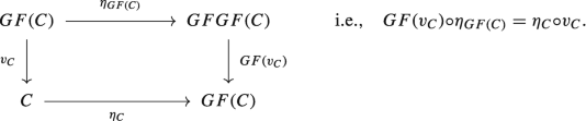
Let$F\colon \mathcal {C} \to \mathcal {D}$and$G\colon \mathcal {D} \to \mathcal {C}$be two functors. Then F is left adjoint to G if and only if there exist two natural transformations

$$\displaystyle \begin{aligned} \eta\colon 1_{\mathcal{C}} \to GF,\qquad \varepsilon\colon FG \to 1_{\mathcal{D}}\end{aligned} $$

such that for all$C \in {Ob} \,\mathcal {C}$and$D \in {\mathrm {Ob}}\, \mathcal {D}$we have

$$\displaystyle \begin{aligned} 1_{F(C)} &= \varepsilon_{F(C)} \circ F \big(\eta_{C}\big) {} \end{aligned} $$

(3.15)

$$\displaystyle \begin{aligned} 1_{G(D)} &= G \big(\varepsilon_{D}\big) \circ \eta_{G(D)}{} \end{aligned} $$

(3.16)

In this case$\eta$and$\varepsilon$are called the unit and the counit of the adjunction, respectively.

Proof

Suppose first that $F \dashv G$ and let $\theta \colon {\mathtt {Hom}}_{\mathcal {D}}(F(-),\, -) \to {\mathtt {Hom}}_{\mathcal {C}}(-,\, G(-))$ be the corresponding natural isomorphism. For each $C \in {\mathrm {Ob}} \,\mathcal {C}$ and $D \in {\mathrm {Ob}}\, \mathcal {D}$ we have the following bijective maps:

$$\displaystyle \begin{aligned} \theta_{C,\, F(C)}&\colon {\mathrm{Hom}}_{\mathcal{D}}(F(C),\, F(C)) \to \mathrm{Hom}_{\mathcal{C}}(C,\,GF(C)),\\ \theta_{G(D),\, D}&\colon {\mathrm{Hom}}_{\mathcal{D}}(FG(D),\, D) \to \mathrm{Hom}_{\mathcal{C}}(G(D),\, G(D)). \end{aligned} $$

Now define $\eta _{C} = \theta _{C,\, F(C)}\big (1_{F(C)}\big )\colon C \to GF(C)$ and $\varepsilon _{D} = \theta _{G(D),\, D}^{-1}\big (1_{G(D)}\big )\colon FG(D)\to D$. We are left to prove (3.15) and (3.16) as well as the naturality of $\eta$ and $\varepsilon$. We start by proving (3.15); indeed, if we consider the commutative diagram (3.1) for $X = GF(C),\ X^{\prime } = C,\ Y = F(C)$ and $f = \eta _{C} \in {\mathrm {Hom}}_{\mathcal {C}}(C,\, GF(C))$ we obtain

From the commutativity of the above diagram applied to

$$\displaystyle \begin{aligned} \varepsilon_{F(C)} \in {\mathrm{Hom}}_{\mathcal{D}}(FGF(C),\,F(C)) \end{aligned} $$

we obtain

$$\displaystyle \begin{aligned} & {\mathtt{Hom}}_{\mathcal{C}}(\eta_{C},\,GF(C))\circ \theta_{GF(C),\,F(C)}(\varepsilon_{F(C)})\\ & \qquad = \theta_{C,\,F(C)} \circ {\mathtt{Hom}}_{\mathcal{D}}(F(\eta_{C}),\,F(C))(\varepsilon_{F(C)})\\ & \qquad \Leftrightarrow \underline{\theta_{GF(C),\,F(C)}(\varepsilon_{F(C)})} \circ \eta_{C} = \theta_{C,\,F(C)}\big(\varepsilon_{F(C)} \circ F(\eta_{C})\big)\\ & \qquad \Leftrightarrow 1_{GF(C)} \circ \eta_{C} = \theta_{C,\,F(C)} \big(\varepsilon_{F(C)} \circ F(\eta_{C})\big)\\ & \qquad \Leftrightarrow \underline{\theta^{-1}_{C,\,F(C)}(\eta_{C})} = \varepsilon_{F(C)} \circ F(\eta_{C})\\ & \qquad \Leftrightarrow 1_{F(C)} = \varepsilon_{F(C)} \circ F(\eta_{C})\,\, {\mathrm{i.e.},}\,\,~(3.15)\,\, {\mathrm{holds}.} \end{aligned} $$

Similarly, by considering the commutative diagram (3.2) for $X = G(D),\ Y = FG(D),\ Y^{\prime } = D$ and $g = \varepsilon _{D} \in {\mathrm {Hom}}_{\mathcal {D}}(FG(D),\, D)$ we get

The commutativity of the above diagram applied to

$$\displaystyle \begin{aligned} 1_{FG(D)} \in {\mathrm{Hom}}_{\mathcal{D}}(FG(D),\,FG(D)) \end{aligned} $$

yields

$$\displaystyle \begin{aligned} & \theta_{G(D),\,D} \circ {\mathtt{Hom}}_{\mathcal{D}}(FG(D),\, \varepsilon_{D})(1_{FG(D)})\\ &\qquad = {\mathtt{Hom}}_{\mathcal{C}}\big(G(D),\,G(\varepsilon_{D})\big) \circ \underline{\theta_{G(D),\,FG(D)}(1_{FG(D)})} \\ &\qquad \Leftrightarrow \theta_{G(D),\,D} \circ {\mathtt{Hom}}_{\mathcal{D}}(FG(D),\, \varepsilon_{D})\circ 1_{FG(D)} = G(\varepsilon_{D}) \circ \eta_{G(D)}\\ &\qquad \Leftrightarrow \underline{\theta_{G(D),\,D}(\varepsilon_{D})} = G(\varepsilon_{D}) \circ \eta_{G(D)}\\ &\qquad \Leftrightarrow 1_{G(D)} = G(\varepsilon_{D}) \circ \eta_{G(D)} \,\, {\mathrm{i.e.,}} \,\,~(3.16)\,\, {\mathrm{holds.}} \end{aligned} $$

Finally, we move on to proving that $\eta$ and $\varepsilon$ are natural transformations. First we will collect some compatibilities using the commutativity of the diagrams (3.1) and (3.2). Setting $X=C,\ X^{\prime }=C^{\prime }$ and $Y = F(C)$ in (3.1) yields the following commutative diagram for all $f \in {\mathrm {Hom}}_{\mathcal {C}}(C^{\prime },\, C)$:

From the commutativity of the above diagram applied to $1_{F(C)}$ we get

$$\displaystyle \begin{aligned} & {\mathtt{Hom}}_{\mathcal{C}}(f,\,GF(C)) \circ \theta_{C,\,F(C)}(1_{F(C)}) = \theta_{C^{\prime},\,F(C)} \circ {\mathtt{Hom}}_{\mathcal{D}}(F(f),\,F(C))(1_{F(C)})\\ & \Leftrightarrow {\mathtt{Hom}}_{\mathcal{C}}(f,\,GF(C)) \circ \eta_{C} = \theta_{C^{\prime},\,F(C)}\big(F(f)\big) \end{aligned} $$

$$\displaystyle \begin{aligned} {} {\mathrm{i.e}.,}\,\, \eta_{C} \circ f = \theta_{C^{\prime},\,F(C)}\big(F(f)\big). \end{aligned} $$

(3.17)

On the other hand, setting $X=C^{\prime },\ Y = F(C^{\prime })$ and $Y^{\prime } = F(C)$ in (3.2) yields the following commutative diagram for all $g \in {\mathrm {Hom}}_{\mathcal {D}}(F(C^{\prime }),\, F(C))$:

By applying the commutativity of the above diagram to $1_{F(C^{\prime })}$ we obtain

$$\displaystyle \begin{aligned} {\mathtt{Hom}}_{\mathcal{C}}(C^{\prime},\,G(g)) \circ \theta_{C^{\prime},\,F(C^{\prime})}(1_{F(C^{\prime})}) = \theta_{C^{\prime},\,F(C)} \circ {\mathtt{Hom}}_{\mathcal{D}}(F(C^{\prime}),\,g)(1_{F(C^{\prime})}), \end{aligned} $$

$$\displaystyle \begin{aligned} {} {\mathrm{i.e}.,}\,\, G(g) \circ \eta_{C^{\prime}} = \theta_{C^{\prime},\,F(C)}(g). \end{aligned} $$

(3.18)

Next we use the commutativity of the diagram (3.1) for $X = G(D),\ X^{\prime } = G(D^{\prime })$ and $Y = D$. It comes down to the following commutative diagram for all $f \in {\mathrm {Hom}}_{\mathcal {C}}(G(D^{\prime }),\,G(D))$:

From the commutativity of the above diagram applied to $\varepsilon _{D}$ we get

$$\displaystyle \begin{aligned} & \theta_{G(D^{\prime}),\,D} \circ {\mathtt{Hom}}_{\mathcal{D}}(F(f),\,D)(\varepsilon_{D}) = {\mathtt{Hom}}_{\mathcal{C}}(f,\,G(D)) \circ \theta_{G(D),\,D}(\varepsilon_{D})\\ & \Leftrightarrow \theta_{G(D^{\prime}),\,D}(\varepsilon_{D} \circ F(f)) = 1_{G(D)} \circ f, \end{aligned} $$

$$\displaystyle \begin{aligned} {} {\mathrm{i.e}.,}\,\, \varepsilon_{D} \circ F(f) = \theta^{-1}_{G(D^{\prime}),\,D}(f). \end{aligned} $$

(3.19)

Finally, we use the commutativity of the diagram (3.2) for $X = G(D^{\prime }),\ Y = D^{\prime }$ and $Y^{\prime } = D$. It yields the following commutative diagram for all $g \in {\mathrm {Hom}}_{\mathcal {D}}(D^{\prime },\,D)$:

The commutativity of the above diagram applied to $\varepsilon _{D^{\prime }}$ gives

$$\displaystyle \begin{aligned} & \theta_{G(D^{\prime}),\,D} \circ {\mathtt{Hom}}_{\mathcal{D}}(FG(D^{\prime}),\,g) (\varepsilon_{D^{\prime}})= {\mathtt{Hom}}_{\mathcal{C}}(G(D^{\prime}),\,G(g)) \circ \theta_{G(D^{\prime}),\,D^{\prime}}(\varepsilon_{D^{\prime}}) \\ & \Leftrightarrow \theta_{G(D^{\prime}),\,D}(g \circ \varepsilon_{D^{\prime}}) = G(g) \circ 1_{G(D^{\prime})}, \end{aligned} $$

$$\displaystyle \begin{aligned} {} {\mathrm{i.e}.,}\,\, g \circ \varepsilon_{D^{\prime}} = \theta^{-1}_{G(D^{\prime}),\,D}\big(G(g)\big). \end{aligned} $$

(3.20)

We are now in a position to prove that $\eta$ and $\varepsilon$ are natural transformations. Indeed, the naturality of $\eta$ comes down to proving the commutativity of the following diagram for all $h \in {\mathrm {Hom}}_{\mathcal {C}}(C^{\prime },\, C)$:

To this end we have

$$\displaystyle \begin{aligned} \eta_{C} \circ h \stackrel{(3.17)}{=} \theta_{C^{\prime},\,F(C)}\big(F(h)\big) \stackrel{(3.18)}{=} GF(h) \circ \eta_{C^{\prime}},\end{aligned} $$

where in the second equality we used (3.18) for $g = F(h)$. Thus $\eta$ is a natural transformation.

The naturality of $\varepsilon$ comes down to proving the commutativity of the following diagram for all $t \in {\mathrm {Hom}}_{\mathcal {D}}(D^{\prime },\,D)$:

which can be proved using (3.19) and respectively (3.20)

$$\displaystyle \begin{aligned} \varepsilon_{D} \circ FG(t) \stackrel{(3.19)}{=} \theta^{-1}_{G(D^{\prime}),\,D} \big(G(t)\big) \stackrel{(3.20)}{=} g \circ \varepsilon_{D^{\prime}}.\end{aligned} $$

Note that the first equality follows by applying (3.19) for $f = G(t)$.

Assume now that there exist two natural transformations $\eta \colon 1_{\mathcal {C}} \to GF$ and $\varepsilon \colon FG \to 1_{\mathcal {D}}$ such that (3.15) and (3.16) are fulfilled for any $C \in {\mathrm {Ob}}\,\mathcal {C}$ and $D \in {\mathrm {Ob}}\,\mathcal {D}$. Define the following maps

$$\displaystyle \begin{aligned} &\theta_{C,\,D}\colon {\mathrm{Hom}}_{\mathcal{D}}(F(C),\, D) \to {\mathrm{Hom}}_{\mathcal{C}}(C,\, G(D)),\quad \theta_{C,\,D}(u) = G(u) \circ \eta_{C},\\ & \varphi_{C,\,D}\colon {\mathrm{Hom}}_{\mathcal{C}}(C,\, G(D)) \to {\mathrm{Hom}}_{\mathcal{D}}(F(C),\, D), \quad \varphi_{C,\,D}(v) = \varepsilon_{D} \circ F(v), \end{aligned} $$

for any $u \in {\mathrm {Hom}}_{\mathcal {D}}(F(C),\, D)$ and $v \in {\mathrm {Hom}}_{\mathcal {C}}(C,\, G(D))$. First we will prove that $\theta _{C,\,D}$ and $\varphi _{C,\,D}$ are inverses to each other for any $C \in {\mathrm {Ob}}\,\mathcal {C}$ and $D \in {\mathrm {Ob}}\,\mathcal {D}$. To start with, we note for further use that the naturality of $\eta$ and $\varepsilon$ imply the commutativity of the following diagrams for all $u \in {\mathrm {Hom}}_{\mathcal {D}}(F(C),\, D)$ and $v \in {\mathrm {Hom}}_{\mathcal {C}}(C,\, G(D))$:

(3.21)

(3.22)

Now, we have

$$\displaystyle \begin{aligned} \theta_{C,\,D} \circ \varphi_{C,\,D}(v) &= \theta_{C,\,D}\big(\varepsilon_{D} \circ F(v)\big) = G\big(\varepsilon_{D} \circ F(v)\big) \circ \eta_{C}\\ &= G(\varepsilon_{D}) \circ \underline{GF(v) \circ \eta_{C}}\\ &\stackrel{(3.21)}{=} \underline{G (\varepsilon_{D}) \circ \eta_{G(D)}} \circ v\\ &\stackrel{(3.16)}{=} v,\\ \varphi_{C,\,D} \circ \theta_{C,\,D}(u)&= \varphi_{C,\,D}\big(G(u) \circ \eta_{C}\big) = \varepsilon_{D} \circ F \big(G(u) \circ \eta_{C}\big)\\ &= \underline{\varepsilon_{D} \circ FG(u)} \circ F(\eta_{C})\\ &\stackrel{(3.22)}{=} u \circ \underline{\varepsilon_{F(C)} \circ F(\eta_{C})}\\ &\stackrel{(3.15)}{=} u. \end{aligned} $$

Thus $\theta _{C,\,D}$ and $\varphi _{C,\,D}$ are inverses to each other for any $C \in {\mathrm {Ob}}\,\mathcal {C}$ and $D \in {\mathrm {Ob}}\,\mathcal {D}$. We are left to prove that $\theta$ is natural in both variables, i.e., diagrams (3.1) and (3.2) are commutative. Indeed, let $f \in {\mathrm {Hom}}_{\mathcal {C}}(C^{\prime },\, C)$ and $u \in {\mathrm {Hom}}_{\mathcal {D}}(F(C),\, D)$; we have

$$\displaystyle \begin{aligned} {\mathtt{Hom}}_{\mathcal{C}}(f,\, G(D)) \circ \theta_{C,\,D}(u) &= {\mathtt{Hom}}_{\mathcal{C}}(f,\, G(D)) \circ \big(G(u) \circ \eta_{C}\big)\\ &= G(u) \circ \underline{\eta_{C} \circ f}\\ &= G(u) \circ GF(f) \circ \eta_{C^{\prime}}\\ &= \theta_{C^{\prime},\,D} \big(u \circ F(f)\big)\\ &= \theta_{C^{\prime},\,D} \circ {\mathtt{Hom}}_{\mathcal{D}} (F(f),\, D)(u), \end{aligned} $$

where in the third equality we used the naturality of $\eta$ applied to f. Thus, (3.1) holds.

Consider now $g \in {\mathrm {Hom}}_{\mathcal {D}}(D,\, D^{\prime })$ and $u \in {\mathrm {Hom}}_{\mathcal {D}}(F(C),\, D)$. Then:

$$\displaystyle \begin{aligned} {\mathtt{Hom}}_{\mathcal{C}}(C,\, G(g)) \circ \theta_{C,\,D}(u) &= G(g) \circ G(u) \circ \eta_{C}\\ &= G(g \circ u) \circ \eta_{C}\\ &= \theta_{C,\,D^{\prime}}\circ {\mathtt{Hom}}_{\mathcal{D}}(F(C),\, g)(u). \end{aligned} $$

This proves that (3.2) also holds and the proof is now finished. □

Examples 3.5.2

• (1) Let $F\colon \mathcal {C} \to \mathcal {D}$ be an isomorphism of categories with inverse $G\colon \mathcal {D} \to \mathcal {C}$. Then $(F,\,G)$ and $(G,\, F)$ are pairs of adjoint functors with unit and counit given by the identity natural transformations. It is straightforward to check that the compatibility conditions (3.15) and (3.16) are trivially fulfilled.

• (2) Consider the pair of adjoint functors $F = - \otimes X$, $G = {\mathtt {Hom}}_{{ }_{K}\mathcal {M}}(X,\, - ) \colon { }_{K}\mathcal {M} \to { }_{K}\mathcal {M}$ from Example 3.4.1, (2) where $\otimes = \otimes _{K}$. The unit and counit of the adjunction $F \dashv G$ are given as follows for any $Y,\ Z \in {\mathrm {Ob}}\,{ }_{K}\mathcal {M}$:

  $$\displaystyle \begin{aligned} & \eta \colon 1_{{}_{K}\mathcal{M}} \to {\mathtt{Hom}}_{{}_{K}\mathcal{M}}(X,\, - \otimes X), \quad \varepsilon \colon {\mathtt{Hom}}_{{}_{K}\mathcal{M}}(X,\, - ) \otimes X \to 1_{{}_{K}\mathcal{M}},\\ & \eta_{Y}\colon Y \to {\mathtt{Hom}}_{{}_{K}\mathcal{M}}(X,\, Y \otimes X),\,\,\, \eta_{Y}(y)(x) = y \otimes x,\, y \in Y, x\in X,\\ & \varepsilon_{Z} \colon {\mathtt{Hom}}_{{}_{K}\mathcal{M}}(X,\, Z) \otimes X \to Z,\,\,\, \varepsilon_{Z}(f \otimes x) \\ &= f(x),\, f \in {\mathrm{Hom}}_{{}_{K}\mathcal{M}}(X,\, Z), x \in X. \end{aligned} $$

  Indeed, for all $x \in X,\ y \in Y$ and $f \in {\mathrm {Hom}}_{{ }_{K}\mathcal {M}}(X,\, Y)$ we have

  $$\displaystyle \begin{aligned} \varepsilon_{Y \otimes X} \circ (\eta_{Y} \otimes 1_{X})(y \otimes x) &= \varepsilon_{Y \otimes X} \big(\eta_{Y}(y) \otimes x\big) \\ &= \eta_{Y}(y)(x) = y \otimes x,\\ {\mathtt{Hom}}_{{}_{K}\mathcal{M}}(X,\, \varepsilon_{Y}) \circ \eta_{{\mathrm{Hom}}_{{}_{K}\mathcal{M}}(X,\, Y)}(f)(x) &= {\mathtt{Hom}}_{{}_{K}\mathcal{M}}(X,\, \varepsilon_{Y})(f \otimes x)\\ & = \varepsilon_{Y}(f \otimes x) = f(x), \end{aligned} $$

  which shows that (3.15) and (3.16) hold true.

• (3) Similarly to the free group functor, we can construct the free module functor$\mathcal {R} \colon {\mathbf {Set}} \to { }_{R}\mathcal {M}$ as follows:

  • for any $X \in {\mathrm {Ob}}\,{\mathbf {Set}}$, define $\mathcal {R}(X) = RX$, the free module generated by X;⁵

  • given $f \in {\mathrm {Hom}}_{{\mathbf {Set}}}(X,\,Y)$, define $\mathcal {R}(f)\colon RX \to RY$ by $\mathcal {R}(f) = \overline {f}$, where $\overline {f}$ is the unique homomorphism of R-modules which makes the following diagram commute:

    

    (3.23)

  where $(RX,\,i_{X})$ and $(RY,\, i_{Y})$ are the free R-modules generated by X and Y , respectively. $\mathcal {R}$ is the left adjoint of the forgetful functor $U \colon { }_{R}\mathcal {M} \to {\mathbf {Set}}$. Indeed, the unit $\eta \colon 1_{{\mathbf {Set}}} \to U\mathcal {R}$ is defined for all $X \in {\mathrm {Ob}}\, {\mathbf {Set}}$ by $\eta _{X} = i_{X}$, where $i_{X} \colon X \to RX$ is the map corresponding to the free R-module on X while the counit $\varepsilon \colon \mathcal {R}U \to 1_{{ }_{R}\mathcal {M}}$ is defined for all $M \in {\mathrm {Ob}}\, { }_{R}\mathcal {M}$ as the unique homomorphism of R-modules $\varepsilon _{M} \colon R(U(M)) \to M$ such that the following diagram is commutative:

  

  (3.24)

  First, note that (3.23) implies in particular that for all $f \in {\mathrm {Hom}}_{{\mathbf {Set}}}(X,\,Y)$ the following diagram is commutative:

  

  In other words, $\eta$ is a natural transformation. By applying U to (3.24) and having in mind that $\eta _{U(M)} = i_{U(M)}$ gives $U(\varepsilon _{M}) \circ \eta _{U(M)} = 1_{U(M)}$, which shows that condition (3.16) is fulfilled. We are left to show that $\varepsilon$ is a natural transformation such that (3.15) also holds. To this end, we have

  $$\displaystyle \begin{aligned} \underline{1_{RX}} \circ i_{X} = \stackrel{(3.24)}{=} \varepsilon_{RX} \circ \underline{i_{U(RX)} \circ i_{X}} \stackrel{(3.23)}{=} \varepsilon_{RX} \circ R(i_{X}) \circ i_{X}. \end{aligned} $$

  This shows that $1_{RX} \circ i_{X} = \varepsilon _{RX} \circ R(i_{X}) \circ i_{X}$ and in light of [45, Definition 1.8] we can conclude that $1_{RX} = \varepsilon _{RX} \circ R(i_{X})$. Hence, (3.15) also holds. Consider now $g \in {\mathrm {Hom}}_{{ }_{R}\mathcal {M}}(M,\,N)$; the proof will be finished once we show the commutativity of the following diagram:

  

  By the same argument used in the above paragraph, it will suffice to show that $g \circ \varepsilon _{M} \circ i_{U(M)} = \varepsilon _{N} \circ RU(g) \circ i_{U(M)}$. Indeed, we have

  $$\displaystyle \begin{aligned} \varepsilon_{N} \circ \underline{RU(g) \circ i_{U(M)}} &\stackrel{(3.23)}{=} \underline{\varepsilon_{N} \circ i_{U(N)}} \circ U(g)\\ &\stackrel{(3.24)}{=} 1_{N} \circ g = g \circ \underline{1_{M}} \stackrel{(3.24)}{=} g \circ \varepsilon_{M} \circ i_{U(M)}, \end{aligned} $$

  as desired.$\square$

We record here for further use the following slightly more general version of the compatibility conditions between the unit and counit of an adjunction:

Lemma 3.5.3

Let$F\colon \mathcal {C} \to \mathcal {D}$and$G\colon \mathcal {D} \to \mathcal {C}$be two functors such that$F \dashv G$and consider the corresponding natural isomorphism$\theta \colon {\mathtt {Hom}}_{\mathcal {D}}(F(-),\, -) \to {\mathtt {Hom}}_{\mathcal {C}}(-,\, G(-))$. If$\eta$and$\varepsilon$are the unit and counit of this adjunction, then for all$u \in {\mathtt {Hom}}_{\mathcal {D}}(F(C),\,D)$and$v \in {\mathrm {Hom}}_{\mathcal {C}}(C,\, G(D))$we have

$$\displaystyle \begin{aligned} \varepsilon_{D} \circ F \big(\theta_{C,\,D}(u)\big) &= u, {} \end{aligned} $$

(3.25)

$$\displaystyle \begin{aligned} G \big(\theta^{-1}_{C,\,D}(v)\big) \circ \,\eta_{C} &= v.{} \end{aligned} $$

(3.26)

Proof

To start with, if we consider the commutative diagram (3.1) for $X = G(D),\ X^{\prime } = C,\ Y = D$ and $f = \theta _{C,\, D}(u)$ we get

From the commutativity of the above diagram applied to $\varepsilon _{D} \in {\mathrm {Hom}}_{\mathcal {D}}(FG(D),\,D)$ we obtain

$$\displaystyle \begin{aligned} & {\mathtt{Hom}}_{\mathcal{C}}(\theta_{C,\,D}(u),\,G(D))\circ \theta_{G(D),\,D}(\varepsilon_{D}) = \theta_{C,\,D} \circ {\mathtt{Hom}}_{\mathcal{D}}\Big(F\big(\theta_{C,\,D}(u)\big),\,D\Big)(\varepsilon_{D})\\ & \Leftrightarrow \underline{\theta_{G(D),\,D}(\varepsilon_{D}) } \circ \theta_{C,\,D}(u) = \theta_{C,\,D}\Big(\varepsilon_{D} \circ F\big(\theta_{C,\,D}(u)\big)\Big)\\ & \Leftrightarrow 1_{G(D)} \circ \theta_{C,\,D}(u) = \theta_{C,\,D}\Big(\varepsilon_{D} \circ F\big(\theta_{C,\,D}(u)\big)\Big)\\ \end{aligned} $$

and the bijectivity of $\theta _{C,\,D}$ shows that (3.25) indeed holds.

For the second identity, consider the commutative diagram (3.2) for $X = C,\ Y = F(C),\ Y^{\prime } = D$ and $g = \theta ^{-1}_{C,\,D}(v) \in {\mathrm {Hom}}_{\mathcal {D}}(F(C),\, D)$

The commutativity of the above diagram applied to $1_{F(C)} \in {\mathrm {Hom}}_{\mathcal {D}}(F(C), F(C))$ yields

$$\displaystyle \begin{aligned} & \theta_{C,\,D} \circ {\mathtt{Hom}}_{\mathcal{D}}(F(C),\, \theta^{-1}_{C,\,D}(v))(1_{F(C)})\\ &\qquad \qquad = {\mathtt{Hom}}_{\mathcal{C}}\Big(C,\,G\big(\theta_{C,\,D}^{-1}(v)\big)\Big) \circ \underline{\theta_{C,\,F(C)}(1_{F(C)})} \\ & \qquad \qquad \Leftrightarrow v = G\big(\theta_{C,\,D}^{-1}(v)\big) \circ\, \eta_{C}, \end{aligned} $$

which shows that (3.26) also holds. □

Corollary 3.5.4

Let$F \colon \mathcal {C} \to \mathcal {D}$and$G \colon \mathcal {D} \to \mathcal {C}$be two functors such that$F \dashv G$and consider$\eta$and$\varepsilon$to be the unit and respectively the counit of this adjunction. Then$\varepsilon ^{\mathit {op}}$and$\eta ^{\mathit {op}}$are the unit and respectively the counit of the adjunction$G^{\mathit {op}} \dashv F^{\mathit {op}}$.

Proof

Indeed, by Theorem 3.5.1 the unit and counit of the adjunction $F \dashv G$ are defined as follows for all $C \in {\mathrm {Ob}}\, \mathcal {C}$ and $D \in {\mathrm {Ob}}\, \mathcal {D}$:

$$\displaystyle \begin{aligned} \eta_{C} = \theta_{C,\, F(C)}\big(1_{F(C)}\big), \,\,\,\, \varepsilon_{D} = \theta_{G(D),\, D}^{-1}\big(1_{G(D)}\big), \end{aligned} $$

where $\theta$ denotes the natural isomorphism induced by the adjunction. Similarly, if $\overline {\eta }$, $\overline {\varepsilon },\ \overline {\theta }$ denote the unit, the counit and respectively the natural isomorphism induced by the adjunction $G^{\mathit {op}} \dashv F^{\mathit {op}}$, we have

$$\displaystyle \begin{aligned} & \overline{\eta}_{D} = \overline{\theta}_{D,\, G^{\mathit{op}}(D)}\Big(1_{G^{\mathit{op}}(D)}^{\mathit{op}}\Big) \stackrel{(3.6)}{=} \Big(\theta^{-1}_{G(D),\, D}\big(1_{G(D)}\big)\Big)^{\mathit{op}} = \varepsilon_{D}^{\mathit{op}},\\ & \overline{\varepsilon}_{C} = \overline{\theta}^{\,-1}_{F^{\mathit{op}}(C),\, C}\Big(1_{F^{\mathit{op}}(C)}^{\mathit{op}}\Big) \stackrel{(3.7)}{=} \Big(\theta_{C,\, F(C)}\big(1_{F(C)}\big)\Big)^{\mathit{op}} = \eta_{C}^{\mathit{op}}, \end{aligned} $$

and the proof is now finished. □

Our next result provides a way of inducing natural transformations between two pairs of adjoint functors.

Theorem 3.5.5

Let$F_{i} \colon \mathcal {C} \to \mathcal {D}$and$G_{i} \colon \mathcal {D} \to \mathcal {C}$be functors such that$F_{i} \dashv G_{i}$and denote by$\theta ^{i}$the corresponding natural isomorphism for all$i =1,\,2$. Then, for any natural transformation$\alpha \colon G_{1} \to G_{2}$there exists a unique natural transformation$\overline {\alpha } \colon F_{2} \to F_{1}$such that the following diagram is commutative for all$C \in {\mathrm {Ob}}\,\mathcal {C}$and$D \in {\mathrm {Ob}}\,\mathcal {D}$:

$$\displaystyle \begin{aligned} {} {\mathrm{i.e}.,}\,\,\,\, \theta^{2}_{C,\,D} \circ {\mathtt{Hom}}_{\mathcal{D}}(\overline{\alpha}_{C},\,D)(f) = {\mathtt{Hom}}_{\mathcal{C}}(C,\,\alpha_{D})\circ \theta^{1}_{C,\,D}(f), \end{aligned} $$

(3.27)

for all$f \in {\mathrm {Hom}}_{\mathcal {D}}(F_{1}(C),\,D)$.

Proof

For all $C \in {\mathrm {Ob}}\, \mathcal {C}$, we denote by $\psi ^{C} \colon {\mathtt {Hom}}_{\mathcal {D}}(F_{1}(C),-) \to {\mathtt {Hom}}_{\mathcal {D}}(F_{2} (C),-)$ the natural transformation defined for all $D \in {\mathrm {Ob}}\, \mathcal {D}$ as the following composition:

$$\displaystyle \begin{aligned} {} \psi^{C}_{D} = \big(\theta^{2}_{C,\,D}\big)^{-1} \circ \,{\mathtt{Hom}}_{\mathcal{C}} (C,\, \alpha_{D}) \circ \theta^{1}_{C,\,D}. \end{aligned} $$

(3.28)

We will show first that each $\psi ^{C}$ is indeed a natural transformation between ${\mathtt {Hom}}_{\mathcal {D}}(F_{1}(C),-)$ and ${\mathtt {Hom}}_{\mathcal {D}}(F_{2}(C),-)$. To this end, we will show that the following diagram is commutative for all $u \in {\mathrm {Hom}}_{\mathcal {D}}(D,\, D^{\prime })$:

$$\displaystyle \begin{aligned} &{\mathrm{i.e}.,}\,\,\,\, u \circ \psi^{C}_{D}(v) = \psi^{C}_{D^{\prime}}(u \circ v)\,\,\, {\mathrm{for}}\,\, {\mathrm{all}}\,\, v \in {\mathrm{Hom}}_{\mathcal{D}}(F_{1}(C),\,D). \end{aligned} $$

Indeed, this can be written equivalently as follows:

$$\displaystyle \begin{aligned} & u \circ \big(\theta^{2}_{C,\,D}\big)^{-1}\big(\alpha_{D} \circ \theta^{1}_{C,\,D}(v)\big) = \big(\theta^{2}_{C,\,D^{\prime}}\big)^{-1}\big(\alpha_{D^{\prime}} \circ \theta^{1}_{C,\,D^{\prime}}(u \circ v)\big)\\ &\Leftrightarrow \underline{\theta^{2}_{C,\,D^{\prime}}\Big(u \circ \big(\theta^{2}_{C,\,D}\big)^{-1}\big(\alpha_{D} \circ \theta^{1}_{C,\,D}(v)\big)\Big)} = \alpha_{D^{\prime}} \circ \theta^{1}_{C,\,D^{\prime}}(u \circ v)\\ &\hspace{-1mm}\stackrel{(3.2)}{\Leftrightarrow} G_{2}(u) \circ \theta^{2}_{C,\,D} \Big( \big(\theta^{2}_{C,\,D}\big)^{-1}\big(\alpha_{D} \circ \theta^{1}_{C,\,D}(v)\big)\Big) = \alpha_{D^{\prime}} \circ \theta^{1}_{C,\,D^{\prime}}(u \circ v)\\ &\Leftrightarrow G_{2}(u) \circ \alpha_{D} \circ \theta^{1}_{C,\,D}(v) = \alpha_{D^{\prime}} \circ \underline{\theta^{1}_{C,\,D^{\prime}}(u \circ v)}\\ &\hspace{-1mm}\stackrel{(3.2)}{\Leftrightarrow} G_{2}(u) \circ \alpha_{D} \circ \theta^{1}_{C,\,D}(v) = \alpha_{D^{\prime}} \circ G_{1}(u) \circ \theta^{1}_{C,\,D}(v), \end{aligned} $$

and the last equality holds because $\alpha \colon G_{1} \to G_{2}$ is a natural transformation, i.e., we have $G_{2}(u) \circ \alpha _{D} = \alpha _{D^{\prime }} \circ G_{1}(u)$ for all $u \in {\mathrm {Hom}}_{\mathcal {D}}(D,\, D^{\prime })$.

This shows that, for each $C \in {\mathrm {Ob}}\, \mathcal {C},\ \psi ^{C}$ is indeed a natural transformation and by Corollary 1.10.4, (1) there exists a unique morphism $\overline {\alpha }_{C} \in {\mathrm {Hom}}_{\mathcal {D}}(F_{2}(C),\,F_{1}(C))$ such that $\psi ^{C}_{D}(f) = f \circ \overline {\alpha }_{C}$ for all $f \in {\mathrm {Hom}}_{\mathcal {D}}(F_{1}(C),\,D)$. In light of (3.28), $\overline {\alpha }_{C} \in {\mathrm {Hom}}_{\mathcal {D}}(F_{2}(C),\,F_{1}(C))$ is the unique morphism such that

$$\displaystyle \begin{aligned} {} \theta^{2}_{C,\,D}(f \circ \overline{\alpha}_{C}) = \alpha_{D} \circ \theta^{1}_{C,\,D}(f),\,\, {\mathrm{for}}\,\,{\mathrm{all}}\,\, f \in {\mathrm{Hom}}_{\mathcal{D}}(F_{1}(C),\,D), \end{aligned} $$

(3.29)

which proves that diagram (3.27) is commutative.

Next we show that $\overline {\alpha } \colon F_{2} \to F_{1}$ defined by (3.27) is in fact a natural transformation, i.e., the following diagram is commutative for all $g \in {\mathrm {Hom}}_{\mathcal {C}}(C,\,C^{\prime })$:

Given the bijectivity of each $\theta ^{2}_{C,\,F_{1}(C^{\prime })}$ it will suffice to prove that the following holds:

$$\displaystyle \begin{aligned} \theta^{2}_{C,\,F_{1}(C^{\prime})}\big(\overline{\alpha}_{C^{\prime}} \circ F_{2}(g)\big) = \theta^{2}_{C,\,F_{1}(C^{\prime})}\big(F_{1}(g) \circ \overline{\alpha}_{C}\big). \end{aligned} $$

To this end, we have

$$\displaystyle \begin{aligned} \underline{\theta^{2}_{C,\,F_{1}(C^{\prime})}\big(F_{1}(g) \circ \overline{\alpha}_{C}\big)} &\stackrel{(3.29)}{=} \alpha_{F_{1}(C^{\prime})} \circ \underline{\theta^{1}_{C,\, F_{1}(C^{\prime})}\big(F_{1}(g)\big)}\\ &\stackrel{(3.17)}{=} \alpha_{F_{1}(C^{\prime})} \circ \underline{\eta^{1}_{C^{\prime}}} \circ g\\ &= \underline{\alpha_{F_{1}(C^{\prime})} \circ \theta^{1}_{C^{\prime},\, F_{1}(C^{\prime})}\big(1_{F_{1}(C^{\prime})}\big)} \circ g\\ &\stackrel{(3.29)}{=} \underline{\theta^{2}_{C^{\prime},\,F_{1}(C^{\prime})}(\overline{\alpha}_{C^{\prime}})\circ g}\\ &\stackrel{(3.1)}{=} \theta^{2}_{C,\,F_{1}(C^{\prime})}\big(\overline{\alpha}_{C^{\prime}} \circ F_{2}(g)\big), \end{aligned} $$

where $\eta ^{1}$ and $\theta ^{1}$ denote the unit and respectively the natural isomorphism induced by the adjunction $F_{1} \dashv G_{1}$. □

Recall that if I is a small category then any functor $F \colon \mathcal {C} \to \mathcal {D}$ induces a functor between the corresponding functor categories $F_{\star } \colon {\mathrm {Fun}\ (\mathrm {I},\, \mathcal {C})} \to {\mathrm {Fun}\ (\mathrm {I},\, \mathcal {D})}$ as in (1.36). Our next result shows that any adjunction can be lifted to an adjunction between the corresponding induced functors.

Proposition 3.5.6

Let$F \colon \mathcal {C} \to \mathcal {D},\ G \colon \mathcal {D} \to \mathcal {C}$be two functors such that$F \dashv G$and I a small category. Then$F_{\star } \dashv G_{\star }$, where$F_{\star } \colon {\mathrm {Fun}\ (\mathrm {I},\, \mathcal {C})} \to {\mathrm {Fun}\ (\mathrm {I},\, \mathcal {D})}$and$G_{\star } \colon {\mathrm {Fun}\ (\mathrm {I},\, \mathcal {D})} \to {\mathrm {Fun}\ (\mathrm {I},\, \mathcal {C})}$are the corresponding induced functors.

Proof

Let $\eta \colon 1_{\mathcal {C}} \to GF$ and $\varepsilon \colon FG \to 1_{\mathcal {D}}$ denote the unit and respectively the counit of the adjunction $F \dashv G$. Consider now the natural transformations $\overline {\eta } \colon 1_{{\mathrm {Fun}\ (\mathrm {I},\, \mathcal {C})}} \to G_{\star }F_{\star }$ and $\overline {\varepsilon } \colon F_{\star }G_{\star } \to 1_{{\mathrm {Fun}\ (\mathrm {I},\, \mathcal {D})}}$ defined for all functors $H \colon I \to \mathcal {C},\ K \colon I \to \mathcal {D}$ by the whiskering of $\eta$ on the left by H and respectively the whiskering of $\varepsilon$ on the left by K (see Example 1.7.2, (7)). More precisely, we have

$$\displaystyle \begin{aligned} \overline{\eta}_{H} = \eta H,\,\,\, \overline{\varepsilon}_{K} = \varepsilon K. \end{aligned} $$

In order to show that $\overline {\eta }$ and $\overline {\varepsilon }$ are indeed natural transformations, consider two natural transformations $\alpha \colon H \to H^{\prime }$ and $\beta \colon K \to K^{\prime }$, where $H,\ H^{\prime } \colon I \to \mathcal {C}$ and K, $K^{\prime } \colon I \to \mathcal {D}$ are functors. First, by the naturality of $\eta$ and $\varepsilon$, the following diagrams are commutative for all $i \in {\mathrm {Ob}}\, I$:

(3.30)

To summarize, for all $i \in {\mathrm {Ob}}\, I$ we obtain

$$\displaystyle \begin{aligned} \big(G_{\star}F_{\star}(\alpha) \circ \overline{\eta}_{H} \big)_{i} &\stackrel{(3.45)}{=} GF(\alpha_{i}) \circ \eta_{H(i)} \stackrel{(3.30)}{=} \eta_{H^{\prime}(i)} \circ \alpha_{i} = (\overline{\eta}_{H^{\prime}} \circ \alpha)_{i},\\ \big(\overline{\varepsilon}_{K^{\prime}} \circ F_{\star}G_{\star}(\beta)\big)_{i} &\stackrel{(3.45)}{=} \varepsilon_{K^{\prime}(i)} \circ FG(\beta_{i}) \stackrel{(3.30)}{=} \beta_{i} \circ \varepsilon_{K(i)} = (\beta \circ \overline{\varepsilon}_{K})_{i}, \end{aligned} $$

which shows that $\overline {\eta }$ and $\overline {\varepsilon }$ are natural transformations. The proof will be finished once we show that $\overline {\eta }$ and $\overline {\varepsilon }$ fulfill (3.15) and (3.16). To start with, note that since $\eta$ and $\varepsilon$ fulfill (3.15) and (3.16), in particular the following hold for all $i \in {\mathrm {Ob}}\, I$:

$$\displaystyle \begin{aligned} 1_{FH(i)} = \varepsilon_{FH(i)} \circ F \big(\eta_{H(i)}\big), \qquad 1_{GK(i)} = G \big(\varepsilon_{K(i)}\big) \circ \eta_{GK(i)}. \end{aligned} $$

The above identities come down to the following:

$$\displaystyle \begin{aligned} 1_{F_{\star}(H)} = \overline{\varepsilon}_{F_{\star}(H)} \circ F_{\star}\big(\overline{\eta}_{H}\big), \qquad 1_{G_{\star}(K)} = G_{\star} \big(\overline{\varepsilon}_{K}\big) \circ \overline{\eta}_{G_{\star}(K)}, \end{aligned} $$

which shows precisely that $\overline {\eta }$ and $\overline {\varepsilon }$ fulfill (3.15) and (3.16) and the proof is now finished. □

3.6 Another Characterisation of Adjoint Functors

A very useful characterization of an adjunction involving only the (co)unit is the following:

Theorem 3.6.1

Let$F\colon \mathcal {C} \to \mathcal {D}$and$G\colon \mathcal {D} \to \mathcal {C}$be two functors. The following are equivalent:

• (1) $F \dashv G$;

• (2) there exists a natural transformation$\eta \colon 1_{\mathcal {C}} \to GF$such that for any morphism$f \in {\mathrm {Hom}}_{\mathcal {C}}(C,\, G(D))$there exists a unique morphism$g \in {\mathrm {Hom}}_{\mathcal {D}}(F(C),\, D)$which makes the following diagram commutative:

  

  (3.31)

• (3) there exists a natural transformation$\varepsilon \colon FG \to 1_{\mathcal {D}}$such that for any morphism$f \in {\mathrm {Hom}}_{\mathcal {D}}(F(C),\, D)$there exists a unique morphism$g \in {\mathrm {Hom}}_{\mathcal {C}}(C,\, G(D))$which makes the following diagram commutative:

  

  (3.32)

As the notation suggests, the natural transformations$\eta$and$\varepsilon$are precisely the unit and the counit, respectively, of the adjunction$F \dashv G$.

Proof

We start by proving the equivalence between (1) and (2). Suppose first that $F \dashv G$ and let $\theta$ be the corresponding natural isomorphism. We define the natural transformation $\eta \colon 1_{\mathcal {C}} \to GF$ as in the proof of Theorem 3.5.1, namely by $\eta _{C} = \theta _{C, F(C)}(1_{F(C)})$ for any $C \in {\mathrm {Ob}}\,\mathcal {C}$. Let $f \in {\mathrm {Hom}}_{\mathcal {C}}(C,\, G(D))$; we will prove that $g = \theta ^{-1}_{C,D}(f) \in {\mathrm {Hom}}_{\mathcal {D}}(F(C),\,D)$ is the unique morphism in $\mathcal {D}$ which makes diagram (3.31) commutative. Indeed, setting $X=C,\ Y = F(C)$ and $Y^{\prime } = D$ in (3.2) gives the following commutative diagram for all $u \in {\mathrm {Hom}}_{\mathcal {C}}(F(C),\, D)$:

By applying the commutativity of the above diagram to $1_{F(C)}$ we obtain

$$\displaystyle \begin{aligned} {\mathtt{Hom}}_{\mathcal{C}}(C,\,G(u)) \circ \theta_{C,\,F(C)}(1_{F(C)}) = \theta_{C,\,D} \circ {\mathtt{Hom}}_{\mathcal{D}}(F(C),\,u)(1_{F(C)}), \end{aligned} $$

$$\displaystyle \begin{aligned} {} {\mathrm{i.e}.,} \,\,\,\, G(u) \circ \eta_{C} = \theta_{C,\,D}(u). \end{aligned} $$

(3.33)

Thus, we have

$$\displaystyle \begin{aligned} G(g) \circ \eta_{C} \stackrel{(3.33)}{=} \theta_{C,D}(g) = \theta_{C,D} \circ \theta^{-1}_{C,D}(f) = f,\end{aligned} $$

which shows that $g = \theta ^{-1}_{C,D}(f) \in {\mathrm {Hom}}_{\mathcal {D}}(F(C),\,D)$ makes diagram (3.31) commutative. Assume now that there exists another morphism $g^{\prime } \in {\mathrm {Hom}}_{\mathcal {D}}(F(C),\,D)$ such that $G(g^{\prime }) \circ \eta _{C} = f$ and let $f^{\prime } = \theta _{C,D}(g^{\prime })$. Following the same steps as in the argument above it can be easily seen that $G(g^{\prime }) \circ \eta _{C} = \theta _{C,D}(g^{\prime }) = f^{\prime }$. Our assumption now implies that $f = f^{\prime }$ and therefore, since $\theta _{C,\,D}$ is a bijection, we obtain $g = g^{\prime }$.

Assume now that $2)$ holds, i.e., for any $f \in {\mathrm {Hom}}_{\mathcal {C}}(C,\, G(D))$ there exists a unique morphism $g \in {\mathrm {Hom}}_{\mathcal {D}}(F(C),\, D)$ such that (3.31) is fulfilled. Given $C \in {\mathrm {Ob}}\, \mathcal {C}$ and $D \in {\mathrm {Ob}}\, \mathcal {D}$ we define the following map:

$$\displaystyle \begin{aligned} {} \theta_{C,\,D}\colon {\mathrm{Hom}}_{\mathcal{D}}(F(C),\, D) \to {\mathrm{Hom}}_{\mathcal{C}}(C,\, G(D)),\quad \theta_{C,\,D}(u) = G(u) \circ \eta_{C} \end{aligned} $$

(3.34)

for any $u \in {\mathrm {Hom}}_{\mathcal {D}}(F(C),\, D)$. Obviously, our assumption implies that $\theta _{C,\,D}$ is a set bijection for all $C \in {\mathrm {Ob}}\, \mathcal {C}$ and $D \in {\mathrm {Ob}}\, \mathcal {D}$. The fact that $\theta$ defined in (3.34) is natural in both variables follows exactly as in the proof of Theorem 3.5.1.

Finally, we are left to show the equivalence between (1) and (3). Indeed, by Theorem 3.4.3, $F \dashv G$ if and only if $G^{\mathit {op}} \dashv F^{\mathit {op}}$. By applying the equivalence between (1) and (2) we obtain that $G^{\mathit {op}} \dashv F^{\mathit {op}}$ if and only if there exists a natural transformation $\overline {\eta } \colon 1_{\mathcal {D}^{\mathit {op}}} \to F^{\mathit {op}}G^{\mathit {op}}$ with the property that for any $f^{\mathit {op}} \in {\mathrm {Hom}}_{\mathcal {D}^{\mathit {op}}}(D,\, F^{\mathit {op}}(C))$ there exists a unique $g^{\mathit {op}} \in {\mathrm {Hom}}_{\mathcal {C}^{\mathit {op}}}(G^{\mathit {op}}(D),\, C)$ such that the following holds:

$$\displaystyle \begin{aligned} {} F^{\mathit{op}}(g^{\mathit{op}}) \circ^{\mathit{op}} \overline{\eta}_{D} = f^{\mathit{op}}. \end{aligned} $$

(3.35)

By Proposition 1.8.3, there exists a natural transformation $\varepsilon \colon FG \to 1_{\mathcal {D}}$ such that $\overline {\eta } = \varepsilon ^{\mathit {op}}$. Now it can be easily seen that (3.35) comes down to $\varepsilon _{D} \circ F(g) = f$. Putting everything together, we obtain that $F \dashv G$ if and only if there exists a natural transformation $\varepsilon \colon FG \to 1_{\mathcal {D}}$ such that for any $f \in {\mathrm {Hom}}_{\mathcal {D}}(D,\, F(C))$ there exists a unique $g \in {\mathrm {Hom}}_{\mathcal {C}}(G(D),\, C)$ such that $\varepsilon _{D} \circ F(g) = f$. The proof is now complete. □

As a straightforward consequence of Theorem 3.6.1 we have:

Corollary 3.6.2

Suppose$F\colon \mathcal {C} \to \mathcal {D}$and$G\colon \mathcal {D} \to \mathcal {C}$are two functors such that$F \dashv G$and let$\eta \colon 1_{\mathcal {C}} \to GF$, $\varepsilon \colon FG \to 1_{\mathcal {D}}$be the unit, respectively the counit of the adjunction.

• (1) If$g,\ g^{\prime } \in {\mathrm {Hom}}_{\mathcal {D}}(F(C),D)$such that$G(g) \circ \eta _{C} = G(g^{\prime }) \circ \eta _{C}$then$g = g^{\prime }$.

• (2) If$h,\ h^{\prime } \in {\mathrm {Hom}}_{\mathcal {C}}(C,G(D))$such that$\varepsilon _{D} \circ F(h) = \varepsilon _{D} \circ F(h^{\prime })$then$h = h^{\prime }$.

Proof

• (1) Follows trivially from Theorem 3.6.1, (2) by considering $f = G(g^{\prime }) \circ \eta _{C}$. Then both morphisms g and $g^{\prime }$ make diagram (3.31) commutative, which implies $g = g^{\prime }$. The second part follows in a similar manner by using Theorem 3.6.1, (3).

□

Examples 3.6.3

• (1) The forgetful functor $U\colon {\mathbf {Top}} \to {\mathbf {Set}}$ has both a left and a right adjoint. We start by constructing the left adjoint functor $F \colon {\mathbf {Set}} \to {\mathbf {Top}}$ which endows each $X \in {\mathrm {Ob}}\, {\mathbf {Set}}$ with the discrete topology. We define a natural transformation $\eta \colon 1_{{\mathbf {Set}}} \to UF$ by $\eta _{X} (x) = x$ for any $X \in {\mathrm {Ob}}\, {\mathbf {Set}}$ and $x \in X$. Consider now $f \in {\mathrm {Hom}}_{{\mathbf {Set}}}(X,\, U(Y))$, where $Y \in {\mathrm {Ob}}\, {\mathbf {Top}}$. According to Theorem 3.6.1, (2) in order to prove that $F \dashv U$ we need to find a unique morphism $g \in {\mathrm {Hom}}_{{\mathbf {Top}}}(F(X),\, Y)$ such that the following diagram commutes:

  

  To this end, it is enough to consider $g = f$. Note that f is obviously continuous since $F(X)$ is endowed with the discrete topology.

  On the other hand, the right adjoint $G \colon {\mathbf {Set}} \to {\mathbf {Top}}$ endows each $X \in {\mathrm {Ob}}\, {\mathbf {Set}}$ with the indiscrete topology. We define a natural transformation $\eta \colon 1_{{\mathbf {Top}}} \to GU$ by $\eta _{X}(x) = x$ for all $X \in {\mathrm {Ob}}\, {\mathbf {Top}}$ and $x \in X$. Now since $\eta ^{-1}_{X}(\emptyset ) = \emptyset$ and $\eta ^{-1}_{X}(G(X)) = G(X) = X$ we obtain that each $\eta _{X}$ is continuous. Consider now $f \in {\mathrm {Hom}}_{{\mathbf {Top}}}(X,\, G(Y))$, where $Y \in {\mathrm {Ob}}\, {\mathbf {Set}}$. We aim to find a unique morphism $g \in {\mathrm {Hom}}_{{\mathbf {Set}}}(U(X),\, Y)$ such that the following diagram is commutative:

  

  As before, we set $g=f$.

• (2) The Stone–Čech compactification functor $\mathcal {S} \colon \mathbf {Top} \to \mathbf {KHaus}$ defined in Example 1.5.3, (24) is left adjoint to the inclusion functor $I\colon \mathbf {KHaus} \to \mathbf {Top}$. Indeed, let $i \colon 1_{ \mathbf {Top}} \to I\mathcal {S}$ be the natural transformation defined for all topological spaces X by the continuous map $i_{X} \colon X \to \mathcal {S}(X)$ associated with the Stone–Čech compactification of X. If $f \in {\mathrm {Hom}}_{{\mathbf {Top}}}(X,\,Y)$ then $\mathcal {S}(f)$ is defined by (1.7) as the unique morphism in $\mathbf {KHaus}$ such that $I\mathcal {S}(f) \circ i_{X} = i_{Y} \circ f$. Therefore, the following diagram is commutative for all $f \in {\mathrm {Hom}}_{{\mathbf {Top}}}(X,\,Y)$:

  

  This shows that i is indeed a natural transformation. Now recall that by the universal property of the Stone–Čech compactification, for any $f \in {\mathrm {Hom}}_{{\mathbf {Top}}}(X,\,I(Z))$, where $Z \in {\mathrm {Ob}}\, {\mathbf {KHaus}}$, there exists a unique $g \in {\mathrm {Hom}}_{{\mathbf {KHaus}}}(\mathcal {S}(X),\,Z)$ such that the following diagram is commutative:

  

  Using Theorem 3.6.1, (2) we can conclude that $\mathcal {S}$ is left adjoint to I, as desired.

• (3) The Grothendieck group functor $\mathcal {G} \colon \mathbf {Mon} \to \mathbf {Grp}$ defined in Example 1.5.3, (25) is left adjoint to the inclusion functor $I \colon \mathbf {Grp} \to \mathbf {Mon}$. Indeed, let $i \colon 1_{ \mathbf {Mon}} \to I\mathcal {G}$ be the natural transformation defined for all monoids M by the homomorphism of monoids $i_{M} \colon M \to I\mathcal {G}(M)$ associated with the Grothendieck group of M. Indeed, if $f \in {\mathrm {Hom}}_{{\mathbf {Mon}}}(M,\,N)$ then $\mathcal {G}(f)$ is defined by (1.8) as the unique morphism in $\mathbf {Grp}$ such that $I\mathcal {G}(f) \circ i_{M} = i_{N} \circ f$. Therefore, the following diagram is commutative for all $f \in {\mathrm {Hom}}_{{\mathbf {Mon}}}(M,\,N)$:

  

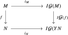
  In particular, this shows that i is indeed a natural transformation. Now using the universal property of the Grothendieck group, for any $f \in {\mathrm {Hom}}_{{\mathbf {Mon}}}(M,\,I(N))$, where $N \in {\mathrm {Ob}}\, {\mathbf {Grp}}$, there exists a unique $g \in {\mathrm {Hom}}_{{\mathbf {Grp}}}(\mathcal {G}(M),\,N)$ such that the following diagram is commutative:

  

  Using Theorem 3.6.1, (2) we can conclude that G is left adjoint to I, as desired.

• (4) The functor $\mathcal {U} \colon \mathbf {Mon} \to \mathbf {Grp}$ defined in Example 1.5.3, (26) which assigns to each monoid its group of invertible elements, is right adjoint to the inclusion functor $I \colon \mathbf {Grp} \to \mathbf {Mon}$. Indeed, let $\varepsilon \colon I\mathcal {U} \to 1_{ \mathbf {Mon}}$ be the natural transformation defined for all $M \in {\mathrm {Ob}}\, \mathbf {Mon}$ by $\varepsilon _{M} \colon U(M) \to M,\ \varepsilon _{M} = i_{M}$, where $i_{M}$ denotes the inclusion map. If $f \in {\mathrm {Hom}}_{{\mathbf {Mon}}}(M,\,N)$, then for all $m \in U(M)$ we have

  $$\displaystyle \begin{aligned} (f \circ i_{M})(m) = f(m) = \big(i_{N} \circ f_{|U(M)}\big)(m) = \big(i_{N} \circ I\mathcal{U}(f)\big)(m).\end{aligned} $$

  Therefore, the following diagram is commutative for all $f \in {\mathrm {Hom}}_{{\mathbf {Mon}}}(M,\,N)$:

  

  which shows that $\varepsilon$ is a natural transformation. Now, if $f \in {\mathrm {Hom}}_{{\mathbf {Mon}}}(I(G), M)$, where $G \in {\mathrm {Ob}}\, \mathbf {Grp}$, then $f(G)$ is also a group and therefore $f(G) \subseteq U(M)$. Hence $f \in {\mathrm {Hom}}_{{\mathbf {Grp}}}(G,\,U(M))$ and f is the unique morphism which makes the following diagram commutative:

  

  Using Theorem 3.6.1, (3) we can conclude that $\mathcal {U}$ is right adjoint to I, as desired.

• (5) Let R be a commutative ring with unity and $(S^{-1}R,\,j)$ its localization with respect to the multiplicative set $S \subset R$, where $j \colon R \to S^{-1}R$ is the ring homomorphism defined by $j(r) = \frac {r}{1}$ for all $r \in R$. Then the localization functor $\mathcal {L} \colon _{R}\mathcal {M} \to { }_{S^{-1}R}\mathcal {M}$ defined in Example 1.5.3, (29) is left adjoint to the restriction of scalars functor $F_{j} \colon _{S^{-1}R}\mathcal {M} \to _{R}\!\!\mathcal {M}$ induced by the ring homomorphism j (see Example 1.5.3, (32)).

  Throughout, if M is an R-module we denote by $(S^{-1}M,\, \varphi _{M})$ its localization module at S. Consider the natural transformation $\varphi \colon 1_{{ }_{R}\mathcal {M}} \to F_{j} \mathcal {L}$ defined for all R-modules M by the R-module homomorphism $\varphi _{M} \colon M \to S^{-1}M$ associated with the localization module $S^{-1}M$. If $f \in {\mathrm {Hom}}_{{ }_{R}\mathcal {M}}(M,\,N)$ then $\mathcal {L}(f)$ is defined by (1.9) to be the unique morphism in ${ }_{S^{-1}R}\mathcal {M}$ such that $\varphi _{N} \circ f = F_{j}\mathcal {L}(f) \circ \varphi _{M}$. Therefore, the following diagram is commutative for all $f \in {\mathrm {Hom}}_{{ }_{R}\mathcal {M}}(M,\,N)$:

  

  In particular, this shows that $\varphi$ is indeed a natural transformation. Now recall that by the universal property of the localization module ([3, Theorem 12.3]), for any $f \in {\mathrm {Hom}}_{{ }_{R}\mathcal {M}}(M,\,F_{j}(N))$, with $N \in {\mathrm {Ob}}\, _{S^{-1}R}\mathcal {M}$, there exists a unique $g \in {\mathrm {Hom}}_{{ }_{S^{-1}R}\mathcal {M}}(\mathcal {L}(M),\,N)$ such that the following diagram is commutative:

  

  Using Theorem 3.6.1, (2) we can now conclude that $\mathcal {L}$ is left adjoint to $F_{j}$, as desired.

• (6) The Hausdorff quotient functor $\mathcal {H} \colon \mathbf {Top} \to \mathbf {Haus}$ defined in Example 1.5.3, (30) is left adjoint to the inclusion functor $I\colon \mathbf {Haus} \to \mathbf {Top}$. Indeed, let $q \colon 1_{ \mathbf {Top}} \to I\mathcal {H}$ be the natural transformation defined for all topological spaces X by the continuous map $q_{X} \colon X \to H(X)$ associated with the Hausdorff quotient of X. If $f \in {\mathrm {Hom}}_{{\mathbf {Top}}}(X,\,Y)$ then $\mathcal {H}(f)$ is defined by (1.10) as the unique morphism in Haus such that $q_{Y} \circ f = I\mathcal {H}(f) \circ q_{X}$. Therefore, the following diagram is commutative for all $f \in {\mathrm {Hom}}_{{\mathbf {Top}}}(X,\,Y)$:

  

  This shows that q is indeed a natural transformation. Now recall that by the universal property of the Hausdorff quotient, for any $f \in {\mathrm {Hom}}_{{\mathbf {Top}}}(X,\,I(Z))$, where $Z \in {\mathrm {Ob}}\, {\mathbf {Haus}}$, there exists a unique $g \in {\mathrm {Hom}}_{{\mathbf {Haus}}}(H(X),\,Z)$ such that the following diagram is commutative:

  

  Using Theorem 3.6.1, (2) we can conclude that $\mathcal {H}$ is left adjoint to I, as desired.

• (7) The Dorroh extension functor $\mathcal {D} \colon {\mathbf {Rng}} \to {\mathbf {Ring}}$ defined in Example 1.5.3, (31) is left adjoint to the inclusion functor $I\colon \mathbf {Ring} \to \mathbf {Rng}$. Indeed, let $j \colon 1_{ \mathbf {Rng}} \to I\mathcal {D}$ be the natural transformation defined for all rings R by the ring homomorphism $j_{R} \colon R \to D(R)$ associated with the Dorroh extension of R. If $f \in {\mathrm {Hom}}_{{\mathbf {Rng}}}(R,\,S)$ then $\mathcal {D}(f)$ is defined by (1.11) as the unique morphism in Ring such that $j_{S} \circ f = I\mathcal {D}(f) \circ j_{R}$. Therefore, the following diagram is commutative for all $f \in {\mathrm {Hom}}_{{\mathbf {Rng}}}(R,\,S)$:

  

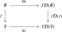
  In particular, this shows that j is a natural transformation. Now recall that by the universal property of the Dorroh extension, for any $f \in {\mathrm {Hom}}_{{\mathbf {Rng}}}(R,\,I(T))$, where $T \in {\mathrm {Ob}}\, {\mathbf {Ring}}$, there exists a unique $g \in {\mathrm {Hom}}_{{\mathbf {Ring}}}(D(R),\,T)$ such that the following diagram is commutative:

  

  Using Theorem 3.6.1, (2) we can conclude that $\mathcal {D}$ is left adjoint to I, as desired. $\square$

As another application of Theorem 3.6.1 we will show that, when they exist, left/right adjoints are unique up to natural isomorphism.

Theorem 3.6.4

Any two left (right) adjoints of a given functor are naturally isomorphic.

Proof

Assume $F,\ F^{\prime }\colon \mathcal {C} \to \mathcal {D}$ are both left adjoint functors of $G\colon \mathcal {D} \to \mathcal {C}$. Then there exist natural transformations $\eta \colon 1_{\mathcal {C}} \to GF$ and $\eta ^{\prime }\colon 1_{\mathcal {C}} \to GF^{\prime }$ satisfying the conditions in Theorem 3.6.1, (2). Given $C \in {\mathrm {Ob}}\, \mathcal {C}$, as $F^{\prime } \dashv G$ and $\eta _{C} \in {\mathrm {Hom}}_{\mathcal {C}}(C,\, GF(C))$, there exists a unique morphism $\gamma _{C} \in {\mathrm {Hom}}_{\mathcal {D}} (F^{\prime }(C),F(C))$ such that

$$\displaystyle \begin{aligned} {} G(\gamma_{C}) \circ \eta^{\prime}_{C} = \eta_{C}. \end{aligned} $$

(3.36)

Similarly, as $F \dashv G$ and $\eta ^{\prime }_{C} \in {\mathrm {Hom}}_{\mathcal {C}}(C,\, GF^{\prime }(C))$, there exists a unique morphism $\gamma ^{\prime }_{C} \in {\mathrm {Hom}}_{\mathcal {D}} (F(C),F^{\prime }(C))$ such that

$$\displaystyle \begin{aligned} {} G(\gamma^{\prime}_{C}) \circ \eta_{C} = \eta^{\prime}_{C}. \end{aligned} $$

(3.37)

We will see that each $\gamma _{C}$ is an isomorphism with the inverse given precisely by $\gamma ^{\prime }_{C}$. Indeed, using (3.36) and (3.37) we can easily see that $G(\gamma ^{\prime }_{C} \circ \gamma _{C}) \circ \eta ^{\prime }_{C} = \eta ^{\prime }_{C}$ and since we obviously also have $G(1_{F^{\prime }(C)}) \circ \eta ^{\prime }_{C} = \eta ^{\prime }_{C}$ it follows by Corollary 3.6.2, (1) that $\gamma ^{\prime }_{C} \circ \gamma _{C} = 1_{F^{\prime }(C)}$. Similarly, one can prove that $\gamma _{C} \circ \gamma ^{\prime }_{C} = 1_{F(C)}$.

We are left to prove that $\gamma \colon F^{\prime } \to F$ is a natural transformation, i.e., for any $f \in {\mathrm {Hom}}_{\mathcal {C}}(C,\,C^{\prime })$ the following diagram is commutative:

Using Corollary 3.6.2, (1) it is enough to prove that the following holds:

$$\displaystyle \begin{aligned} {} G(F(f) \circ \gamma_{C}) \circ \eta^{\prime}_{C} = G(\gamma_{C^{\prime}} \circ F^{\prime}(f)) \circ \eta^{\prime}_{C}. \end{aligned} $$

(3.38)

To this end, we use the naturality of $\eta$ and respectively $\eta ^{\prime }$; that is, the commutativity of the following diagrams:

(3.39)

(3.40)

Then, we have

$$\displaystyle \begin{aligned} GF(f) \circ \underline{G(\gamma_{C}) \circ \eta^{\prime}_{C}} &\stackrel{(3.36)}{=} \underline{GF(f) \circ \eta_{C}}\\ &\stackrel{(3.39)}{=} \underline{\eta_{C^{\prime}}} \circ f\\ &\stackrel{(3.36)}{=} G(\gamma_{C^{\prime}}) \circ \underline{\eta^{\prime}_{C^{\prime}} \circ f}\\ &\stackrel{(3.40)}{=} G(\gamma_{C^{\prime}}) \circ GF^{\prime}(f) \circ \eta^{\prime}_{C}. \end{aligned} $$

Therefore, (3.38) indeed holds. To summarize, we have proved that there exists a natural isomorphism $\gamma \colon F^{\prime } \to F$ and the proof is now finished. □

Adjunctions can also be used to easily derive important properties of certain functorial constructions, as the following examples show. This includes, for instance, the commutation of tensor products or localizations with direct sums of modules. All of these are obtained by applying Theorem 3.4.4.

Example 3.6.5

Given a commutative ring R, for any $X \in {\mathrm {Ob}}_{R}\mathcal {M}$ and any family $(M_{i})_{i \in I}$ of R-modules we have the following isomorphisms of R-modules:

$$\displaystyle \begin{aligned} \big(\oplus_{i \in I}\, M_{i}\big) \otimes X &\simeq \big(\oplus_{i \in I}\, M_{i} \otimes X \big),\\ S^{-1}\big(\oplus_{i \in I}\, M_{i}\big) &\simeq \oplus_{i \in I}\,S^{-1}M_{i}, \end{aligned} $$

where $\otimes = \otimes _{R}$. Indeed, both statements are consequences of the fact that both the tensor product functor $- \otimes X \colon { }_{R}\mathcal {M} \to { }_{R}\mathcal {M}$ and the localization functor $\mathcal {L} \colon _{R}\mathcal {M} \to _{S^{-1}R}\mathcal {M}$ are left adjoints (see Example 3.4.1, (2) and Example 3.6.3, (5)) and therefore they preserve coproducts (see Example 2.1.5, (12)). $\square$

We end this section with the following useful result:

Lemma 3.6.6

Let$F\colon \mathcal {C} \to \mathcal {D},\ G\colon \mathcal {D} \to \mathcal {C}$be two functors such that$F \dashv G$and let$\eta \colon 1_{\mathcal {C}} \to GF$and$\varepsilon \colon FG \to 1_{\mathcal {D}}$be the unit and counit of the adjunction, respectively.

• (1) F is faithful if and only if$\eta _{C}$is a monomorphism for all$C \in {\mathrm {Ob}}\, \mathcal {C}$; G is faithful if and only if$\varepsilon _{D}$is an epimorphism for all$D \in {\mathrm {Ob}}\, \mathcal {D}$;

• (2) F is full if and only if$\eta _{C}$is a split epimorphism for all$C \in {\mathrm {Ob}}\, \mathcal {C}$; G is full if and only if$\varepsilon _{D}$is a split monomorphism for all$D \in {\mathrm {Ob}}\, \mathcal {D}$;

• (3) F is fully faithful if and only if the unit of the adjunction is a natural isomorphism; G is fully faithful if and only if the counit of the adjunction is a natural isomorphism.

Proof

• (1) Assume first that F is faithful and let $f_{1},\ f_{2} \in {\mathrm {Hom}}_{\mathcal {C}}(C^{\prime },\,C)$ such that $\eta _{C} \circ f_{1} = \eta _{C} \circ f_{2}$. Applying F to the last identity yields $F(\eta _{C}) \circ F(f_{1}) = F(\eta _{C}) \circ F(f_{2})$ and after composing on the left with $\varepsilon _{F(C)}$ and using (3.15) we obtain $F(f_{1}) = F(f_{2})$. As F is faithful we arrive at $f_{1} = f_{2}$, which shows that $\eta _{C}$ is indeed a monomorphism.

  Conversely, assume $\eta _{C}$ is a monomorphism for all $C \in {\mathrm {Ob}}\, \mathcal {C}$ and let $f_{1},\ f_{2} \in {\mathrm {Hom}}_{\mathcal {C}}(C^{\prime },\,C)$ such that $F(f_{1}) = F(f_{2})$. Using (3.15) we obtain $\varepsilon _{F(C)} \circ F(\eta _{C} \circ f_{1}) = \varepsilon _{F(C)} \circ F(\eta _{C} \circ f_{2})$. Now Corollary 3.6.2, (2) implies $\eta _{C} \circ f_{1} = \eta _{C} \circ f_{2}$ and since $\eta _{C}$ is a monomorphism we obtain $f_{1} = f_{2}$. Therefore, F is faithful.

  The result concerning the functor G follows by duality. Indeed, by Theorem 3.4.3 we have $G^{\mathit {op}} \dashv F^{\mathit {op}}$ and moreover, Corollary 3.5.4 shows that the unit of this adjunction is precisely $\varepsilon ^{\mathit {op}}$. Since G is faithful if and only if $G^{\mathit {op}}$ is faithful, the desired conclusion follows the first part of the proof and Proposition 1.4.3, (1).

• (2) Let F be a full functor and $C \in {\mathrm {Ob}}\, \mathcal {C}$. Then $\varepsilon _{F(C)} \in {\mathrm {Hom}}_{\mathcal {D}}(FGF(C), F(C))$ and since F is full there exists a morphism $u_{C} \in {\mathrm {Hom}}_{\mathcal {C}}(GF(C),\,C)$ such that $\varepsilon _{F(C)} = F(u_{C})$. We obtain

  $$\displaystyle \begin{aligned} \varepsilon_{F(C)} \circ F(\eta_{C} \circ u_{C}) &= \underline{\varepsilon_{F(C)} \circ F(\eta_{C})} \circ F(u_{C}) \stackrel{(3.15)}{=} F(u_{C})\\ &= \varepsilon_{F(C)} = \varepsilon_{F(C)} \circ F\big(1_{GF(C)}\big) \end{aligned} $$

  Now Corollary 3.6.2, (2) implies $\eta _{C} \circ u_{C} = 1_{GF(C)}$, as desired.

  Conversely, assume $\eta _{C}$ is a split epimorphism for all $C \in {\mathrm {Ob}}\, \mathcal {C}$. Thus, there exists a morphism $v_{C} \in {\mathrm {Hom}}_{\mathcal {C}}(GF(C),\, C)$ such that $\eta _{C} \circ v_{C} = 1_{GF(C)}$. Let $g \in {\mathrm {Hom}}_{\mathcal {D}}(F(C),\,F(C^{\prime }))$. The naturality of $\eta$ applied to $v_{C}$ renders the following diagram commutative:

  

  (3.41)

  Therefore, for all $C \in {\mathrm {Ob}}\, \mathcal {C}$, we obtain

  $$\displaystyle \begin{aligned} GF(v_{C}) \circ \eta_{GF(C)} \stackrel{(3.41)}{=} \eta_{C} \circ v_{C} = 1_{GF(C)} \stackrel{(3.16)}{=} G(\varepsilon_{F(C)}) \circ \eta_{GF(C)}. \end{aligned} $$

  Now Corollary 3.6.2, (1) implies $F(v_{C}) = \varepsilon _{F(C)}$. Finally, the naturality of $\varepsilon$ applied to g yields

  

  (3.42)

  Putting all this together we obtain

  $$\displaystyle \begin{aligned} g = g \circ \underline{1_{F(C)}} &\stackrel{(3.15)}{=} \underline{g \circ \varepsilon_{F(C)}} \circ F(\eta_{C})\\ &\stackrel{(3.42)}{=} \underline{\varepsilon_{F(C^{\prime})}} \circ FG(g) \circ F(\eta_{C}) = F\big(v_{C^{\prime}} \circ G(g) \circ \eta_{C}\big), \end{aligned} $$

  which shows that F is full.

  The result concerning the functor G follows again by duality. Indeed, by Theorem 3.4.3 we have $G^{\mathit {op}} \dashv F^{\mathit {op}}$ and, moreover, Corollary 3.5.4 shows that the unit of this adjunction is precisely $\varepsilon ^{\mathit {op}}$. Since G is full if and only if $G^{\mathit {op}}$ is full, the desired conclusion follows from Exercise 1.6.

• (3) Using (1) and (2), F is fully faithful if and only if $\eta _{C}$ is both a monomorphism and a split epimorphism for all $C \in {\mathrm {Ob}}\, \mathcal {C}$. Similarly, G is fully faithful if and only if $\varepsilon _{D}$ is both an epimorphism and a split monomorphism and for all $D \in {\mathrm {Ob}}\, \mathcal {D}$. The conclusion now follows from Exercise 1.6, (b).

□

3.7 (Co)reflective Subcategories

This section is devoted to a special kind of adjunction, namely those for which one of the functors involved is an inclusion.

Definition 3.7.1

A full subcategory $\mathcal {A}$ of $\mathcal {B}$ is called reflective if the inclusion functor $I\colon \mathcal {A} \to \mathcal {B}$ admits a left adjoint, called a reflector. Dually, a full subcategory $\mathcal {A}$ of $\mathcal {B}$ is called coreflective if the inclusion functor admits a right adjoint, called a coreflector.

We have already encountered many examples of such subcategories:

Examples 3.7.2

• (1) Ab is a reflective subcategory of Grp, as shown in Example 3.4.1, (4).

• (2) Grp is both a reflective and a coreflective subcategory of Mon as shown in Example 3.6.3, (3) and (4).

• (3) KHaus is a reflective subcategory of Top. The Stone–Čech compactification provides the reflector, as shown in Example 3.6.3, (2).

• (4) Haus is a reflective subcategory of Top. The Hausdorff quotient provides the reflector, as shown in Example 3.6.3, (6).

• (5) Ring is not a reflective subcategory of Rng. Indeed, note that although the inclusion functor $I \colon {\mathbf {Ring}} \to {\mathbf {Rng}}$ has a left adjoint, as shown in Example 3.6.3, (7) the category Ring is not a full subcategory of Rng.$\square$

One important feature of (co)reflective subcategories is that they behave well with respect to (co)limits. The remaining of this section will be devoted to studying their (co)completeness and providing explicit descriptions of the (co)limits.

Proposition 3.7.3

Let$\mathcal {A}$be a subcategory of$\mathcal {B}$.

• (1) If$\mathcal {A}$is a reflective subcategory of the complete category$\mathcal {B}$then$\mathcal {A}$is itself complete.

• (2) If$\mathcal {A}$is a coreflective subcategory of the cocomplete category$\mathcal {B}$then$\mathcal {A}$is itself cocomplete.

Proof

• (1) Let $R\colon \mathcal {B} \to \mathcal {A}$ be the reflector of the inclusion functor $I\colon \mathcal {A} \to \mathcal {B}$, i.e., $R \dashv I$. Let J be a small category and $F\colon J \to \mathcal {A}$ a functor. Since $\mathcal {B}$ is complete, the functor $IF\colon J \to \mathcal {B}$ has a limit, which we denote by $\big (L,\, (p_{j}\colon L \to IF(j))_{j \in {\mathrm {Ob}}\, J}\big )$. Since $\big (L,\, (p_{j}\colon L \to IF(j))_{j \in {\mathrm {Ob}}\, J}\big )$ is in particular a cone on IF, the following diagram is commutative for all $d \in {\mathrm {Hom}}_{J}(j,\,l)$:

  

  (3.43)

  Let $\eta \colon 1_{\mathcal {B}} \to IR$ be the unit of the adjunction $R \dashv I$ (see Theorem 3.5.1). By Theorem 3.6.1, (2) for any $p_{j} \in {\mathrm {Hom}}_{\mathcal {B}}(L,\,IF(j))$ there exists a unique morphism $q_{j} \in {\mathrm {Hom}}_{\mathcal {A}}(R(L),\,F(j))$ such that the following diagram commutes for all $j \in {\mathrm {Ob}}\, J$:

  

  (3.44)

  We will prove first that $\big (R(L),\, (q_{j}\colon R(L) \to F(j))_{j \in {\mathrm {Ob}}\, J}\big )$ is a cone on F. Indeed, for all $d \in {\mathrm {Hom}}_{J}(j,\,l)$ we have

  $$\displaystyle \begin{aligned} I\big(F(d) {\circ} q_{j}\big) {\circ} \eta_{L} {=} IF(d) {\circ} \underline{I\big(q_{j}\big) \circ \eta_{L}} \stackrel{(3.44)}{=}\hspace{-1pt} IF(d) \,{\circ}\, p_{j} \stackrel{(3.43)}{=}\hspace{-2pt} p_{l} \stackrel{(3.44)}{=} I\big(q_{l}\big) {\circ}\, \eta_{L}. \end{aligned} $$

  Now by Corollary 3.6.2, (1) we get $F(d) \circ q_{j} = q_{l}$, i.e.,

  $$\displaystyle \begin{aligned} \big(R(L),\, (q_{j}\colon R(L) \to F(j))_{j \in {\mathrm{Ob}}\, J}\big) \end{aligned} $$

  is a cone on F. We will show that $\big (R(L),\, (q_{j})_{j \in {\mathrm {Ob}}\, J}\big )$ is in fact the limit of F.

  We start by showing that $\eta _{L} \colon L \to IR(L)$ is an isomorphism. Indeed, since $\big (IR(L),\, (I(q_{j})\colon IR(L) \to IF(j))_{j \in {\mathrm {Ob}}\, J}\big )$ is a cone on IF by Lemma 2.5.5 and $\big (L,\, (p_{j}\colon L \to IF(j))_{j \in {\mathrm {Ob}}\, J}\big )$ is its limit, there exists a unique morphism $f \in {\mathrm {Hom}}_{\mathcal {B}}(IR(L),\,L)$ such that the following diagram is commutative for all $j \in {\mathrm {Ob}}\, J$:

  

  (3.45)

  Thus, for any $j \in {\mathrm {Ob}}\, J$ we have $\underline {p_{j} \circ f} \circ \eta _{L} \stackrel {(3.45)}{=} I(q_{j}) \circ \eta _{L} \stackrel {(3.44)}{=} p_{j} = p_{j} \circ 1_{L}$ and using Proposition 2.2.14, (1) we obtain

  $$\displaystyle \begin{aligned} {} f \circ \eta_{L} = 1_{L}. \end{aligned} $$

  (3.46)

  On the other hand $\eta _{L} \circ f \in {\mathrm {Hom}}_{\mathcal {B}}(IR(L),\, IR(L))$ and since $I\colon \mathcal {A} \to \mathcal {B}$ is fully faithful, there exists a unique morphism $t \in {\mathrm {Hom}}_{\mathcal {A}}(R(L),\, R(L))$ such that

  $$\displaystyle \begin{aligned} {} \eta_{L} \circ f = I(t). \end{aligned} $$

  (3.47)

  Moreover, we have

  $$\displaystyle \begin{aligned} \underline{I(t)} \circ \eta_{L} \stackrel{(3.47)}{=} \eta_{L} \circ \underline{f \circ \eta_{L}} \stackrel{(3.46)}{=} \eta_{L} = I(1_{R(L)}) \circ \eta_{L}. \end{aligned} $$

  Using again Corollary 3.6.2, (1) we get $t = 1_{R(L)}$ and hence $\eta _{L} \circ f = 1_{IR(L)}$, so $\eta _{L}$ is an isomorphism, as desired.

  Consider now another cone $\big (L^{\prime },\, (t_{j}\colon L^{\prime } \to F(j))_{j \in {\mathrm {Ob}} \, J}\big )$ on F. Then $\big (I(L^{\prime }),\, (I(t_{j})_{j \in {\mathrm {Ob}} \, J}\big )$ is a cone on IF. Therefore, there exists a unique morphism $g \in {\mathrm {Hom}}_{\mathcal {B}}(I(L^{\prime }),\, L)$ such that the following diagram is commutative for all $j \in {\mathrm {Ob}}\, J$:

  

  (3.48)

  Since we also have $p_{j} = I(q_{j}) \circ \eta _{L}$ for all $j \in {\mathrm {Ob}}\, J$, we obtain

  $$\displaystyle \begin{aligned} {} I(q_{j}) \circ \eta_{L} \circ g = I(t_{j}). \end{aligned} $$

  (3.49)

  As $\eta _{L} \circ g \in {\mathrm {Hom}}_{\mathcal {B}}(I(L^{\prime }),\, IR(L))$ and I is fully faithful, there exists a unique morphism $h \in {\mathrm {Hom}}_{\mathcal {A}}(L^{\prime },\, R(L))$ such that $I(h) = \eta _{L} \circ g$. Then (3.49) becomes $I(q_{j} \circ h) = I(t_{j})$ and since I is fully faithful we get $q_{j} \circ h = t_{j}$ for all $j \in {\mathrm {Ob}}\, J$, i.e., the following diagram is commutative:

  

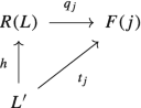
  The proof will be finished once we show that h is the unique morphism which makes the above diagram commutative. Indeed, suppose there exists an $\overline {h} \in {\mathrm {Hom}}_{\mathcal {A}}(L^{\prime },\, R(L))$ such that $q_{j} \circ \overline {h} = t_{j}$ for all $j \in {\mathrm {Ob}}\, J$. Then we also have $I(q_{j}) \circ I(\overline {h}) = I(t_{j})$ and using (3.44) and respectively (3.48) we get

  $$\displaystyle \begin{aligned} p_{j} \circ \eta_{L}^{-1} \circ I(\overline{h}) = p_{j} \circ g \end{aligned} $$

  for all $j \in {\mathrm {Ob}}\, J$. Proposition 2.2.14, (1) implies $\eta _{L}^{-1} \circ I(\overline {h}) = g$ and thus $I(\overline {h}) = \eta _{L} \circ g$. Since h is the unique morphism such that $I(h) = \eta _{L} \circ g$, we get $\overline {h} = h$. This shows that $\big (R(L),\, (q_{j})_{j \in {\mathrm {Ob}}\, J}\big )$ is indeed the limit of F and therefore $\mathcal {A}$ is a complete category.

• (2) Let $\mathcal {A}$ be a coreflective subcategory of a cocomplete category $\mathcal {B}$ and denote by $C \colon \mathcal {B} \to \mathcal {A}$ the right adjoint of the inclusion functor $I \colon \mathcal {A} \to \mathcal {B}$ and by $\varepsilon$ the counit of this adjunction. Let J be a small category and $F\colon J \to \mathcal {A}$ a functor.

  Then $\mathcal {A}^{\mathit {op}}$ is obviously a subcategory of $\mathcal {B}^{\mathit {op}}$ and the inclusion functor is precisely $I^{\mathit {op}}$. Theorem 3.4.3 implies that $C^{\mathit {op}} \dashv I^{\mathit {op}}$ and, moreover, as proved in Corollary 3.5.4, $\varepsilon ^{\mathit {op}}$ is the unit of this adjunction. Using the first part of the proof, the limit of the functor $F^{\mathit {op}} \colon J^{\mathit {op}} \to \mathcal {A}^{\mathit {op}}$ is given by the pair

  $$\displaystyle \begin{aligned} \Big(C(L),\, (q_{j}^{\mathit{op}} \in {\mathrm{Hom}}_{\mathcal{A}^{\mathit{op}}}(C(L),\, F(j^{\mathit{op}})))_{i \in {\mathrm{Ob}}\, J}\Big), \end{aligned} $$

  where $q_{j}^{\mathit {op}}$ is the unique morphism which makes the following diagram commutative:

  

  and $\Big (L,\, (p_{j}^{\mathit {op}} \in {\mathrm {Hom}}_{\mathcal {B}^{\mathit {op}}}(L,\, I^{\mathit {op}}F^{\mathit {op}}(j)))_{i \in {\mathrm {Ob}}\, J}\Big )$ is the limit of the functor $I^{\mathit {op}}F^{\mathit {op}} \colon J^{\mathit {op}} \to \mathcal {B}^{\mathit {op}}$. In other words, for all $j \in {\mathrm {Ob}}\, J,\ q_{j}$ is the unique morphism in $\mathcal {A}$ such that $\varepsilon _{L} \circ I(q_{j})=p_{j}$. Now we can conclude by Lemma 2.2.12 that $\Big (C(L),\, (q_{j} \in {\mathrm {Hom}}_{\mathcal {A}}(F(j),\, C(L)))_{i \in {\mathrm {Ob}}\, J}\Big )$ is the colimit of the functor F and therefore $\mathcal {A}$ is cocomplete.

□

In light of Proposition 3.7.3 the next natural question we are led to consider concerns the cocompleteness of reflective subcategories (and, dually, the completeness of coreflective subcategories).

Proposition 3.7.4

Let$\mathcal {A}$be a subcategory of$\mathcal {B}$.

• (1) If$\mathcal {A}$is a reflective subcategory of a cocomplete category$\mathcal {B}$then$\mathcal {A}$is also cocomplete.

• (2) If$\mathcal {A}$is a coreflective subcategory of a complete category$\mathcal {B}$then$\mathcal {A}$is also complete.

Proof

• (1) Let $I\colon \mathcal {A} \to \mathcal {B}$ be the inclusion functor and $R\colon \mathcal {B} \to \mathcal {A}$ the reflector. Let $F\colon J \to \mathcal {A}$ be a functor, where J is a small category. Since $\mathcal {B}$ is cocomplete, the functor $IF\colon J \to \mathcal {B}$ has a colimit, which we denote by

  $$\displaystyle \begin{aligned} \big(D,\, (q_{j}\colon IF(j) \to D)_{j \in {\mathrm{Ob}}\, J}\big). \end{aligned} $$

  R is left adjoint to I and by Theorem 3.4.4 it preserves colimits, so

  $$\displaystyle \begin{aligned} \big(R(D),\, (R(q_{j})\colon RIF(j) \to R(D))_{j \in {\mathrm{Ob}}\, J}\big) \end{aligned} $$

  is the colimit of the functor $RIF\colon J \to \mathcal {A}$. By Lemma 3.6.6, (3) we know that the counit $\varepsilon \colon RI \to 1_{\mathcal {A}}$ of the adjunction $R \dashv I$ is a natural isomorphism. Therefore, the natural transformation $\varepsilon _{F}\colon RIF \to F$ defined by

  $$\displaystyle \begin{aligned} (\varepsilon_{F})_{j} = \varepsilon_{F(j)}\,\, {\mathrm{for}\,\, \mathrm{all}}\,\, j \in {\mathrm{Ob}}\, J\end{aligned} $$

  is also a natural isomorphism (Example 1.7.2, (7)). Now, in light of Lemma 2.2.15, (2) we can conclude that $\big (R(D),\, (R(q_{j}) \circ \varepsilon ^{-1}_{F(j)}\colon F(j) \to R(D))_{j \in {\mathrm {Ob}}\, J}\big )$ is the colimit of F.

• (2) Let $I\colon \mathcal {A} \to \mathcal {B}$ to be the inclusion functor and denote by $C\colon \mathcal {B} \to \mathcal {A}$ the coreflector and by $\eta$ the unit of this adjunction, which is a natural isomorphism by Lemma 3.6.6, (3). Let $F\colon J \to \mathcal {A}$ be a functor, where J is a small category.

  By Theorem 3.4.3 we also have an adjunction $C^{\mathit {op}} \dashv I^{\mathit {op}}$ whose counit is precisely $\eta ^{\mathit {op}}$. This shows, in particular, that $\mathcal {A}^{\mathit {op}}$ is a reflective subcategory of the cocomplete category $\mathcal {B}^{\mathit {op}}$ with inclusion functor $I^{\mathit {op}}$. By part $1)$ proved above, the colimit of the functor $F^{\mathit {op}}$ is given by the pair

  $$\displaystyle \begin{aligned} \Big(C^{\mathit{op}}(D),\, (C^{\mathit{op}}(q_{j}^{\mathit{op}}) \circ ^{\mathit{op}} (\eta^{-1}_{F^{\mathit{op}}(j)})^{\mathit{op}} \in {\mathrm{Hom}}_{\mathcal{A}^{\mathit{op}}}(F^{\mathit{op}}(j),\, C^{\mathit{op}}(D)))_{j \in {\mathrm{Ob}}\, J}\Big), \end{aligned} $$

  where $\big (D,\, (q^{\mathit {op}}_{j})_{j \in {\mathrm {Ob}}\, J}\big )$ is the colimit of the functor $I^{\mathit {op}}F^{\mathit {op}} \colon J^{\mathit {op}} \to \mathcal {B}^{\mathit {op}}$. Now Lemma 2.2.12 implies that $\big (C(D),\, (\eta ^{-1}_{F(j)} \circ C(q_{j}))_{j \in {\mathrm {Ob}}\, J}\big )$ is the limit of the functor F.

□

3.8 Equivalence of Categories

When studying categories which are practically the same, the first notion we usually encounter is that of an isomorphism of categories, as introduced in Definition 1.6.6. However, this concept turns out to be too strict, as there are many examples of categories with similar properties (such as completeness, cocompleteness etc.) which are not isomorphic. To express that two categories share many of the same properties, a more suitable notion than isomorphism is the following:

Definition 3.8.1

A functor $F\colon \mathcal {C} \to \mathcal {D}$ is called an equivalence of categories and the category $\mathcal {C}$ is said to be equivalent to $\mathcal {D}$ if there exists another functor $G\colon \mathcal {D} \to \mathcal {C}$ such that we have natural isomorphisms $GF \cong 1_{\mathcal {C}}$ and $FG \cong 1_{\mathcal {D}}$. A contravariant functor $F\colon \mathcal {C} \to \mathcal {D}$ for which $F\colon \mathcal {C}^{\mathit {op}} \to \mathcal {D}$ is an equivalence of categories is called a duality of categories.

Example 3.8.2

Given a field K, the category $\mathbf {Mat}_{K}$ defined in Example 1.2.2, (19) is equivalent to the category of finite-dimensional K-vector spaces ${ }_{K}\mathcal {M}^{fd}$. Indeed, the functor $F\colon \mathbf {Mat}_{K} \to { }_{K}\mathcal {M}^{fd}$ defined below is an equivalence of categories:

$$\displaystyle \begin{aligned} &F(n) = K^{n},\mbox{ the }n\mbox{-dimensional space of column vectors over }K\mbox{ for all } n\in {\mathbb N},\\ &F(A) = M_{A},\mbox{ for all morphisms }A\colon m \to n\mbox{ in }\mathbf{Mat}_{K},\mbox{ where } M_{A} \colon K^{m} \to K^{n}\mbox{ is}\\ &\mbox{given by }M_{A}(v)=Av\mbox{ for all } v \in K^{m}. \end{aligned} $$

To this end, we choose a basis⁶$\mathcal {B}_{V}$ for each finite dimensional vector space V  and we define a functor $G \colon { }_{K}\mathcal {M}^{fd} \to \mathbf {Mat}_{K}$ as follows:

$$\displaystyle \begin{aligned} &G(V) = {\mathrm{dim}}(V),\mbox{ for all finite-dimensional vector spaces } V,\\ &G(\alpha) = U_{\alpha},\mbox{ where } U_{\alpha}\mbox{ is the matrix of the linear map } \alpha\colon V \to W\mbox{ with respect to}\\ &\mbox{the chosen bases }\mathcal{B}_{V}\mbox{ and }\mathcal{B}_{W}\mbox{ of }V\mbox{ and }W\mbox{ respectively.} \end{aligned} $$

Throughout this example, by convention, the basis we consider on $K^{n}$ will be the standard basis. We start by showing that $GF = 1_{\mathbf {Mat}_{K}}$. First, for any $n \in {\mathbb N}$ we have

$$\displaystyle \begin{aligned} GF(n) = G\big(K^{n}\big) = {\mathrm{dim}}\big(K^{n}\big) = n = 1_{\mathbf{Mat}_{K}}(n).\end{aligned} $$

Moreover, if $A\colon m \to n$ is a morphism in $\mathbf {Mat}_{K}$, we have $GF(A) = G(M_{A}) = U_{M_{A}}$, where $U_{M_{A}}$ is the matrix of the linear map $M_{A} \colon K^{m} \to K^{n}$ given by $M_{A}(v) = Av$ with respect to the standard bases $\{e_{1},\, e_{2},\, \ldots ,\, e_{m}\}$ and $\{f_{1},\, f_{2},\, \ldots ,\, f_{n}\}$ of $K^{m}$ and $K^{n}$, respectively. Having in mind that the element $e_{i}$ (resp. $f_{j}$) of the standard basis is the column vector in $K^{m}$ (resp. in $K^{n}$) with 1 on the i-th (resp. j-th) position and zeros elsewhere for all $i = 1,\, 2,\, \ldots , m$ (resp. $j = 1,\, 2,\, \ldots ,\, n$), we obtain $M_{A}(e_{i}) = Ae_{i} = \sum _{j=1}^{n}\, a_{ji}\, f_{j}$, where $A = \big (a_{k l}\big )_{k = \overline {1,\,n},\,l = \overline {1,\,m}}$. This proves that $U_{M_{A}} = A$, i.e., $GF(A) = A$, as desired. Hence, we have proved that $GF = 1_{\mathbf {Mat}_{K}}$, which shows that, in particular, GF is naturally isomorphic to $1_{\mathbf {Mat}_{K}}$.

We are left to show that FG is naturally isomorphic to $1_{{ }_{K}\mathcal {M}^{fd}}$. Consider $\eta \colon 1_{{ }_{K}\mathcal {M}^{fd}} \to FG$ defined for any vector space V  by $\eta _{V} \colon V \to K^{{\mathrm {dim}}(V)},\ \eta _{V}(v) = [v]$, where we denote by $[v]$ the (column) coordinate vector of v with respect to the chosen basis of V . We claim that $\eta$ is a natural isomorphism. To start with, each $\eta _{V}$ is clearly a linear bijection. We are left to check the naturality condition. To this end, let $\alpha \colon V \to W$ be a morphism in ${ }_{K}\mathcal {M}^{fd}$ and consider the chosen bases $\mathcal {B}_{V} = \{t_{1},\, t_{2},\, \ldots ,\, t_{m}\}$ and $\mathcal {B}_{W} = \{w_{1},\, w_{2},\, \ldots ,\, w_{n}\}$ in V  and W, respectively, where $m = {\mathrm {dim}}(V),\ n = {\mathrm {dim}}(W)$. The proof will be finished once we show that the following diagram is commutative:

(3.50)

If we define $U_{\alpha } = \big (u_{k l}\big )_{k = \overline {1,\,n},\,l = \overline {1,\,m}}$, then for any $v = \sum _{i=1}^{m} v_{i} \, t_{i} \in V$ we have $\alpha (v) = \sum _{i=1}^{m} v_{i} \, \alpha (t_{i}) = \sum _{i=1}^{m} v_{i} \, \big (\sum _{j=1}^{n} \, u_{ji}\, w_{j}\big ) = \sum _{j=1}^{n} \, \big (\sum _{i=1}^{m} \, v_{i}\, u_{ji}\big )\, w_{j}$. This shows that the j-th component of the column vector $[\alpha (v)]$ is $\sum _{i=1}^{m} \, v_{i}\, u_{ji}$, for all $j = 1,\, 2,\, \ldots ,\, n$. Moreover, a similar straightforward computation shows that the j-th component of $U_{\alpha } [v]$ is $\sum _{i=1}^{m}\, u_{ji}\, v_{i}$ for all $j = 1,\, 2,\, \ldots ,\, n$. Putting everything together we have

$$\displaystyle \begin{aligned} {} [\alpha(v)] = U_{\alpha} [v]. \end{aligned} $$

(3.51)

Therefore, for any $v \in V$, we have

$$\displaystyle \begin{aligned} FG(\alpha) \circ \eta_{V}(v) = FG(\alpha)\big([v]\big) = M_{U_{\alpha}}\big([v]\big) = U_{\alpha}\, [v] \stackrel{(3.51)}{=} \big[\alpha(v)\big] = \eta_{W} \circ \alpha(v), \end{aligned} $$

which proves the commutativity of diagram (3.50). $\square$

Remark 3.8.3

The categories $\mathbf {Mat}_{K}$ and ${ }_{K}\mathcal {M}^{fd}$ from the previous example are equivalent but not isomorphic. Indeed, this follows easily by noticing that $\mathbf {Mat}_{K}$ is a small category while ${ }_{K}\mathcal {M}^{fd}$ has a class of objects.

Proposition 3.8.4

Let$\mathcal {A},\ \mathcal {B}$and$\mathcal {C}$be three categories. The following hold:

• (1) any category is equivalent to itself;

• (2) if$\mathcal {A}$is equivalent to$\mathcal {B}$then$\mathcal {B}$is equivalent to$\mathcal {A}$;

• (3) if$\mathcal {A}$is equivalent to$\mathcal {B}$and$\mathcal {B}$is equivalent to$\mathcal {C}$then$\mathcal {A}$is equivalent to$\mathcal {C}$.

Proof

• (1) Any category $\mathcal {A}$ is equivalent to itself as the identity functor $1_{\mathcal {A}} \colon \mathcal {A} \to \mathcal {A}$ is obviously an equivalence of categories.

• (2) Assume that the category $\mathcal {A}$ is equivalent to $\mathcal {B}$ and $F \colon \mathcal {A} \to \mathcal {B}$ is the equivalence functor. Then there exists another functor $G \colon \mathcal {B} \to \mathcal {A}$ and two natural isomorphisms $GF \cong 1_{\mathcal {A}}$ and $FG \cong 1_{\mathcal {B}}$. This shows that G is also an equivalence of categories and therefore $\mathcal {B}$ is equivalent to $\mathcal {A}$.

• (3) Assume that $\mathcal {A}$ is equivalent to $\mathcal {B}$ and $\mathcal {B}$ is equivalent to $\mathcal {C}$. Then, we have two pairs of functors and their corresponding natural isomorphisms

  $$\displaystyle \begin{aligned} & F \colon \mathcal{A} \to \mathcal{B},\,\,\, G \colon \mathcal{B} \to \mathcal{A},\,\,\,\,\,\, \alpha \colon FG \to 1_{\mathcal{B}},\,\,\, \beta \colon GF \to 1_{\mathcal{A}},\\ & H \colon \mathcal{B} \to \mathcal{C},\,\,\, T \colon \mathcal{C} \to \mathcal{B},\,\,\,\,\,\, \gamma \colon HT \to 1_{\mathcal{C}},\,\,\, \sigma \colon TH \to 1_{\mathcal{B}}. \end{aligned} $$

  Consider now the functors $HF \colon \mathcal {A} \to \mathcal {C}$ and $GT \colon \mathcal {C} \to \mathcal {A}$ and the following natural transformations obtained by whiskering $\alpha$ and $\sigma$ as in Example 1.7.2, (7) both on the left and on the right:

  

  Note that the above natural transformations are in fact natural isomorphisms since $\alpha _{T}$ and $\sigma _{F}$ are natural isomorphisms (Example 1.7.2, (7)) and all functors preserve isomorphisms (Proposition 1.6.9, (1)). This gives rise to the following natural isomorphisms:

  

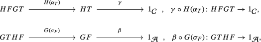
  and we can now conclude that $\mathcal {A}$ is equivalent to $\mathcal {C}$.

□

We have the following very useful characterization of equivalences of categories:

Theorem 3.8.5

Let$F\colon \mathcal {C} \to \mathcal {D}$be a functor. The following are equivalent:

• (1) F is an equivalence of categories;

• (2) F is fully faithful and essentially surjective;

• (3) there exists a right adjoint$G\colon \mathcal {D} \to \mathcal {C}$of F such that the unit and counit of the adjunction are natural isomorphisms;

• (4) there exists a left adjoint$G \colon \mathcal {D} \to \mathcal {C}$of F such that the unit and counit of the adjunction are natural isomorphisms.

In particular, as the notation suggests, an equivalence of categories has a left adjoint which is also a right adjoint and the unit and counit of these adjunctions are natural isomorphisms.

Proof

• (1)⇒(2) Since F is an equivalence of categories, there exists a functor $G\colon \mathcal {D} \to \mathcal {C}$ and two natural isomorphisms $\eta \colon 1_{\mathcal {C}} \to GF$ and $\varepsilon \colon FG \to 1_{\mathcal {D}}$. To start with, for any $D \in {\mathrm {Ob}}\,\mathcal {D}$ the morphism $\varepsilon _{D} \in {\mathrm {Hom}}_{\mathcal {D}}(FG(D),\, D)$ is an isomorphism and therefore F is essentially surjective. Next we prove that F is fully faithful. Let $h_{1},\ h_{2} \in {\mathrm {Hom}}_{\mathcal {C}}(C,\,C^{\prime })$ such that $F(h_{1})=F(h_{2})$. Then we also have $GF(h_{1})=GF(h_{2})$. Moreover, the naturality of $\eta$ renders the following diagrams commutative:

  

  (3.52)
  

  (3.53)

  From (3.52) and (3.53) we obtain $\eta _{C^{\prime }} \circ h_{1} = \eta _{C^{\prime }} \circ h_{2}$ and since $\eta _{C^{\prime }}$ is an isomorphism we get $h_{1} = h_{2}$, as desired. Similarly, using the naturality of $\varepsilon$ it follows that G is faithful as well.

  Consider now $C,\ C^{\prime } \in {\mathrm {Ob}}\, \mathcal {C}$ and $g \in {\mathrm {Hom}}_{\mathcal {D}}(F(C),\,F(C^{\prime }))$. Now define

  $$\displaystyle \begin{aligned} {} f = \eta_{C^{\prime}}^{-1} \circ G(g) \circ \eta_{C} \in {\mathrm{Hom}}_{\mathcal{C}}(C,\,C^{\prime}). \end{aligned} $$

  (3.54)

  We will prove that $F(f) = g$. Indeed, using the naturality of $\eta$ applied to f, we obtain

  $$\displaystyle \begin{aligned} \eta_{C^{\prime}}^{-1} \circ GF(f) \circ \eta_{C} \stackrel{(3.52)}{=} f \stackrel{(3.54)}{=} \eta_{C^{\prime}}^{-1} \circ G(g) \circ \eta_{C}. \end{aligned} $$

  Since $\eta _{C}$ and $\eta _{C^{\prime }}$ are isomorphisms, we get $GF(f) = G(g)$. As G is faithful, the above equality comes down to $F(f) = g$, which proves that F is full as well.

• (2)⇒(1) Assume now that F is fully faithful and essentially surjective. First note that since F is fully faithful it reflects isomorphisms (see Proposition 1.6.9, (2)) and therefore two objects C and $C^{\prime }$ are isomorphic in $\mathcal {C}$ if and only if $F(C)$ and $F(C^{\prime })$ are isomorphic in $\mathcal {D}$. Therefore, as F is essentially surjective, for any $D \in {\mathrm {Ob}}\,\mathcal {D}$ there exists a unique (up to isomorphism) $C \in {\mathrm {Ob}}\, \mathcal {C}$ such that $F(C) \simeq D$. Thus, for any $D \in {\mathrm {Ob}}\, \mathcal {D}$ we can choose⁷ an object $G(D) \in {\mathrm {Ob}}\, \mathcal {C}$ and an isomorphism $\varepsilon _{D}\colon FG(D) \to D$ in $\mathcal {D}$. Now if $g \in {\mathrm {Hom}}_{\mathcal {D}}(D,\,D^{\prime })$ we have the following morphism in $\mathcal {D}$:

  $$\displaystyle \begin{aligned} \varepsilon_{D^{\prime}}^{-1} \circ g \circ \varepsilon_{D}\colon FG(D) \to FG(D^{\prime}).\end{aligned} $$

  Since F is fully faithful, there exists a unique morphism $G(g) \in {\mathrm {Hom}}_{\mathcal {C}}(G(D),\,G(D^{\prime }))$ such that $FG(g) = \varepsilon _{D^{\prime }}^{-1} \circ g \circ \varepsilon _{D}$. The last equality implies the commutativity of the following diagram:

  

  (3.55)

  We will prove that G defined above is in fact a functor and $\varepsilon \colon FG \to 1_{\mathcal {D}}$ is a natural transformation. Indeed, setting $D = D^{\prime }$ and $g = 1_{D}$ yields

  $$\displaystyle \begin{aligned} \varepsilon_{D}^{-1} \circ 1_{D} \circ \varepsilon_{D} = 1 _{FG(D)}\colon FG(D) \to FG(D)\end{aligned} $$

  and there exists a unique morphism $G(1_{D}) \in {\mathrm {Hom}}_{\mathcal {C}}(G(D),\,G(D))$ such that $FG(1_{D}) = 1_{FG(D)} = F(1_{G(D)})$ where the last equality holds because F is a functor. Since F is faithful we get $G(1_{D}) = 1_{G(D)}$. Consider now $g \in {\mathrm {Hom}}_{\mathcal {D}}(D,\,D^{\prime }),\ g^{\prime } \in {\mathrm {Hom}}_{\mathcal {D}}(D^{\prime },\,D^{\prime \prime })$ and the unique morphisms $G(g) \in {\mathrm {Hom}}_{\mathcal {C}}(G(D), G(D^{\prime }))$, respectively $G(g^{\prime }) \in {\mathrm {Hom}}_{\mathcal {C}}(G(D^{\prime }),\,G(D^{\prime \prime }))$ such that

  $$\displaystyle \begin{aligned} FG(g) = \varepsilon^{-1}_{D^{\prime}} \circ g \circ \varepsilon_{D} \quad {\mathrm{and}} \quad FG(g^{\prime}) = \varepsilon^{-1}_{D^{\prime\prime}} \circ g^{\prime} \circ \varepsilon_{D^{\prime}} .\end{aligned} $$

  This yields

  $$\displaystyle \begin{aligned} {} F\big(G(g^{\prime}) \circ G(g)\big) = \varepsilon^{-1}_{D^{\prime\prime}} \circ g^{\prime} \circ g \circ \varepsilon_{D}. \end{aligned} $$

  (3.56)

  Now having in mind that there exists a unique morphism $G(g^{\prime } \circ g) \in {\mathrm {Hom}}_{\mathcal {C}}(G(D),\,G(D^{\prime \prime }))$ such that $FG(g^{\prime }\circ g) = \varepsilon _{D^{\prime \prime }}^{-1} \circ (g^{\prime } \circ g) \circ \varepsilon _{D}$, it follows from (3.56) that $G(g^{\prime }\circ g) = G(g^{\prime })\circ G(g)$. Therefore, G is indeed a functor. Now the commutativity of diagram (3.55) implies that $\varepsilon$ is a natural transformation. Recall that every $\varepsilon _{D}$ is an isomorphism and thus $\varepsilon$ is in fact a natural isomorphism. We are left to construct a natural isomorphism $\eta \colon 1_{\mathcal {C}} \to GF$. For any $C \in {\mathrm {Ob}}\, \mathcal {C}$ we have $\varepsilon _{F(C)}^{-1} \in {\mathrm {Hom}}_{\mathcal {D}}(F(C),\, FGF(C))$, an isomorphism in $\mathcal {D}$. Since F is fully faithful, there exists a unique $\eta _{C} \in {\mathrm {Hom}}_{\mathcal {C}}(C,\,GF(C))$ such that $F(\eta _{C}) = \varepsilon ^{-1}_{F(C)}$. Obviously, $\eta _{C}$ is an isomorphism for all $C \in {\mathrm {Ob}}\, \mathcal {C}$ since F reflects isomorphisms. We prove now that $\eta$ is a natural transformation. To this end, let $f \in {\mathrm {Hom}}_{\mathcal {C}}(C,\, C^{\prime })$; we need to prove the commutativity of the following diagram:

  

  (3.57)

  By naturality of $\varepsilon$ applied to $F(f)$ we have the following commutative diagram:

  
  $$\displaystyle \begin{aligned} {\mathrm{i.e}.,} \quad &\varepsilon_{F(C^{\prime})} \circ FGF(f) = F(f) \circ \varepsilon_{F(C)}\\ & \Leftrightarrow FGF(f) \circ \varepsilon_{F(C)}^{-1} = \varepsilon_{F(C^{\prime})}^{-1} \circ F(f) \\ & \Leftrightarrow FGF(f) \circ F(\eta_{C}) = F(\eta_{C^{\prime}}) \circ F(f)\\ & \Leftrightarrow F\big(GF(f) \circ \eta_{C}\big) = F(\eta_{C^{\prime}} \circ f). \end{aligned} $$

  Since F is faithful we get $GF(f) \circ \eta _{C} = \eta _{C^{\prime }} \circ f$, i.e., (3.57) is commutative, as desired.

• (3)⇒(1) Obvious.

• (1)⇒(3) Suppose F is an equivalence of categories and let $G\colon \mathcal {D} \to \mathcal {C}$ such that $GF \cong 1_{\mathcal {C}}$ and $FG \cong 1_{\mathcal {D}}$. We will prove that G is right adjoint to F. Denote by $\varepsilon \colon FG \to 1_{\mathcal {D}}$ the natural isomorphism arising from the above equivalence. Thus, for any $C \in {\mathrm {Ob}}\, \mathcal {C}$ the morphism $\varepsilon _{F(C)} \in {\mathrm {Hom}}_{\mathcal {D}}(FGF(C),\, F(C))$ is an isomorphism. Therefore, $\varepsilon ^{-1}_{F(C)} \in {\mathrm {Hom}}_{\mathcal {D}}(F(C),\, FGF(C))$ and since F is fully faithful (see $(1) \Rightarrow (2)$) there exists a unique morphism $\eta _{C} \in {\mathrm {Hom}}_{\mathcal {C}}(C,\, GF(C))$ such that $F(\eta _{C}) = \varepsilon ^{-1}_{F(C)}$. Since F is fully faithful, it reflects isomorphisms; thus $\eta _{C}$ is also an isomorphism. Furthermore, one can show exactly as in the proof of $(2) \Rightarrow (1)$ that $\eta$ is also a natural transformation. In light of Theorem 3.5.1, the proof will be finished once we show that (3.15) and (3.16) hold. To start with, for all $C \in {\mathrm {Ob}}\,\mathcal {C}$ we have

  $$\displaystyle \begin{aligned} \varepsilon_{F(C)} \circ F(\eta_{C}) = \varepsilon_{F(C)} \circ \varepsilon^{-1}_{F(C)} = 1_{F(C)}, \quad {\mathrm{i.e}.,}\,\,~(3.15)\,\, {\mathrm{is} \,\, \mathrm{fulfilled}.}\end{aligned} $$

  Consider now $D \in {\mathrm {Ob}}\,\mathcal {D}$ and $\varepsilon ^{-1}_{D} \colon D \to FG(D)$. From the naturality of $\varepsilon$ applied to the morphism $\varepsilon ^{-1}_{D}$ we obtain the following commutative diagram:

  

  Therefore, since F is faithful, we have

  $$\displaystyle \begin{aligned} & FG(\varepsilon_{D}) \circ \varepsilon_{FG(D)}^{-1} = 1_{FG(D)}\\ & \Leftrightarrow FG(\varepsilon_{D}) \circ F(\eta_{G(D)}) = 1_{FG(D)}\\ & \Leftrightarrow F(G(\varepsilon_{D}) \circ \eta_{G(D)} ) = F\big(1_{G(D)}\big)\\ & \Leftrightarrow G(\varepsilon_{D}) \circ \eta_{G(D)} = 1_{G(D)},\quad {\mathrm{i.e}.,}\,\,\,(3.16)\,\, {\mathrm{holds}\,\, \mathrm{as}\,\, \mathrm{well}.} \end{aligned} $$

• (3)⇒(4) Assume now that $G \colon \mathcal {D} \to \mathcal {C}$ is a functor such that $F \dashv G$ and the unit $\eta \colon 1_{\mathcal {C}} \to GF$ and counit $\varepsilon \colon FG \to 1_{\mathcal {D}}$ of this adjunction are natural isomorphisms. Then $G \dashv F$ with unit $\varepsilon ^{-1} \colon 1_{\mathcal {D}} \to FG$ and counit $\eta ^{-1} \colon GF \to 1_{\mathcal {C}}$. Indeed, as $\eta$ and $\varepsilon$ are natural isomorphisms, the compatibility conditions (3.15) and (3.16) imply that for all $C \in {\mathrm {Ob}}\, \mathcal {C}$ and $D \in {\mathrm {Ob}}\, \mathcal {D}$ we have

  $$\displaystyle \begin{aligned} \varepsilon^{-1}_{F(C)} = F(\eta_{C}), \quad \eta^{-1}_{G(D)} = G(\varepsilon_{D}). \end{aligned} $$

  Therefore, for all $C \in {\mathrm {Ob}}\, \mathcal {C}$ and $D \in {\mathrm {Ob}}\, \mathcal {D}$ we have

  $$\displaystyle \begin{aligned} 1_{G(D)} &= \eta^{-1}_{G(D)} \circ G\big(\varepsilon^{-1}_{D}\big),\\ 1_{F(C)} &= F\big(\eta^{-1}_{C}\big)\, \circ\, \varepsilon^{-1}_{F(C)}, \end{aligned} $$

  which shows that the compatibility conditions (3.15) and (3.16) are fulfilled for $\varepsilon ^{-1}$ and $\eta ^{-1}$.

• (4)⇒(3) Follows in the same fashion as $3) \Rightarrow 4)$. The proof is now finished.

□

As an application of the previous theorem we will highlight an equivalence of categories involving ring localizations.

Example 3.8.6

Let R be a commutative ring with unity and $(S^{-1}R,\,j)$ its localization at the multiplicative set $S \subset R$. We will show, using Theorem 3.8.5, (2) that the category ${ }_{S^{-1}R}\mathcal {M}$ of modules over the localization ring $S^{-1}R$ is equivalent to the category ${ }_{R}\mathcal {M}^{S{{{-}}{\mathrm {aut}}}}$ of modules over R on which S acts as automorphisms (see Example 1.2.2, (14)).

Indeed, consider the restriction of scalars functor $F_{j} \colon _{S^{-1}R}\mathcal {M} \to _{R}\!\!\mathcal {M}$ induced by the ring homomorphism $j \colon R \to S^{-1}R$ as defined in Example 1.5.3, (32). First note that since $j \colon R \to S^{-1}R$ is an epimorphism in ${\mathbf {Ring}}^{c}$ (see Example 1.3.2, (5)), the corresponding restriction of scalars functor $F_{j}$ is fully faithful, as proved in Example 1.6.2, (6).

Furthermore, one can easily show that S acts as automorphisms on $F_{j}(M)$, for any $S^{-1}R$-module M. Indeed, it is straightforward to see that for all $s \in S$ the inverse of the multiplication map $\mu _{s} \colon M \to M,\ \mu _{s}(m) = sm$ is given by the R-linear homomorphism $\mu _{\frac {1}{s}}$, where the juxtaposition denotes the R-module structure on $F_{j}(M) = M$. This proves that the image of the restriction of scalars functor $F_{j}$ is contained in the category ${ }_{R}\mathcal {M}^{S{{{-}}{\mathrm {aut}}}}$.

Therefore, we have a fully faithful functor $F_{j} \colon _{S^{-1}R}\mathcal {M} \to { }_{R}\mathcal {M}^{S{{{-}}{\mathrm {aut}}}}$. We are left to show that $F_{j}$ is essentially surjective as well. To this end, let $M \in {\mathrm {Ob}}\, { }_{R}\mathcal {M}^{S{{{-}}{\mathrm {aut}}}}$. Then M admits an $S^{-1}R$-module structure defined for all $r \in R,\ s \in S$ and $m \in M$ as follows:

$$\displaystyle \begin{aligned} {} \frac{r}{s} \star m = rn, \end{aligned} $$

(3.58)

where the juxtaposition denotes the R-module structure on M and n is the unique element of M such that $sn = m$. Note that the existence and uniqueness of the element n with this property is a consequence of M being an R-module on which S acts as an automorphism. Moreover, if $M \in {\mathrm {Ob}}\, { }_{S^{-1}R}\mathcal {M}$ with the $S^{-1}R$-module structure given in (3.58) then $F_{j}(M)$ has the R-module structure defined as follows for all $r \in R$ and $m \in M$:

$$\displaystyle \begin{aligned} j(r) \star m = \frac{r}{1} \star m = rm, \end{aligned} $$

i.e., it coincides with the initial R-module structure on M. This finishes the proof. $\square$

As stated in the beginning, equivalent categories share most of the important properties:

Proposition 3.8.7

Let$\mathcal {C}$and$\mathcal {D}$be two equivalent categories. Then$\mathcal {C}$is (co)complete if and only if$\mathcal {D}$is (co)complete.

Proof

Given an equivalence of categories $F \colon \mathcal {C} \to \mathcal {D}$, by Theorem 3.8.5, (3) there exists a right adjoint $G \colon \mathcal {D} \to \mathcal {C}$ of F such that the unit $\eta \colon 1_{\mathcal {C}} \to GF$ and the counit $\varepsilon \colon FG \to 1_{\mathcal {D}}$ of the adjunction are natural isomorphisms. Assume first that $\mathcal {D}$ is complete and let $H \colon J \to \mathcal {C}$ be a functor, where J is a small category. As $\mathcal {D}$ is a complete category, the functor $FH \colon J \to \mathcal {D}$ has a limit, say $\big (L,\, (p_{j} \colon L \to FH(j))_{j \in {\mathrm {Ob}}\, J}\big )$. Moreover, as G is right adjoint to F, Theorem 3.4.4 implies that $\big (G(L),\, (G(p_{j}) \colon G(L) \to GFH(j))_{j \in {\mathrm {Ob}}\, J}\big )$ is the limit of the functor $GFH \colon J \to \mathcal {C}$. Now $\eta ^{-1} \colon GF \to 1_{\mathcal {C}}$ (as defined in Example 1.7.2, (6)) is a natural isomorphism and consequently $\eta ^{-1}_{H} \colon GFH \to H$ (as defined in Example 1.7.2, (7)) is also a natural isomorphism. Now Lemma 2.2.15, (1) implies that $\big (G(L),\, (\eta ^{-1}_{H(j)} \circ G(p_{j}) \colon G(L) \to H(j))_{j \in {\mathrm {Ob}}\, J}\big )$ is the limit of H and therefore the category $\mathcal {C}$ is complete.

The statement concerning cocompleteness follows similarly using Theorem 3.8.5, (4). □

Definition 3.8.8

A skeleton of a category $\mathcal {C}$ is a full subcategory $\mathcal {C}_{0}$ of $\mathcal {C}$ such that each object of $\mathcal {C}$ is isomorphic to exactly one object of $\mathcal {C}_{0}$.

Example 3.8.9

A skeleton of a given category $\mathcal {C}$ always exists; indeed, it can be constructed by choosing⁸ an object from each isomorphism class of objects in $\mathcal {C}$ and considering the full subcategory of $\mathcal {C}$ with this objects class. $\square$

Moreover, as an easy consequence of Theorem 3.8.5 we obtain the following:

Corollary 3.8.10

A category is equivalent to any of its skeletons.

Proof

Let $\mathcal {C}_{0}$ be a skeleton of a given category $\mathcal {C}$. Then the inclusion functor $I\colon \mathcal {C}_{0} \to \mathcal {C}$ is fully faithful and essentially surjective. The conclusion now follows from Theorem 3.8.5, (2). □

Proposition 3.8.11

Let$\mathcal {C}_{0}$and$\mathcal {D}_{0}$be two skeletons of the categories$\mathcal {C}$and$\mathcal {D}$, respectively. Then$\mathcal {C}$and$\mathcal {D}$are equivalent if and only if$\mathcal {C}_{0}$and$\mathcal {D}_{0}$are isomorphic.

Proof

Assume first that the categories $\mathcal {C}_{0}$ and $\mathcal {D}_{0}$ are isomorphic; in particular, the two categories are also equivalent. Moreover, recall that the categories $\mathcal {C}_{0}$ and $\mathcal {C}$, respectively $\mathcal {D}_{0}$ and $\mathcal {D}$, are equivalent. Then Proposition 3.8.4, (2) and (3) show that $\mathcal {C}$ is equivalent to $\mathcal {D}$.

Conversely, assume now that $\mathcal {C}$ and $\mathcal {D}$ are equivalent. As noted before, $\mathcal {C}_{0}$ and $\mathcal {C}$, respectively $\mathcal {D}_{0}$ and $\mathcal {D}$, are also equivalent and using again Proposition 3.8.4, (2) and (3) we obtain that $\mathcal {C}_{0}$ and $\mathcal {D}_{0}$ are equivalent too. Thus, there exist two functors $F \colon \mathcal {C}_{0} \to \mathcal {D}_{0},\ G \colon \mathcal {D}_{0} \to \mathcal {C}_{0}$ and two natural isomorphisms $\psi \colon FG \to 1_{\mathcal {D}_{0}},\ \varphi \colon GF \to 1_{\mathcal {C}_{0}}$. Hence, for each $C \in {\mathrm {Ob}}\, \mathcal {C}_{0}$, we have an isomorphism $\varphi _{C} \colon GF(C) \to C$. Since $\mathcal {C}_{0}$ is a skeleton of $\mathcal {C}$, such an isomorphism can only be an identity morphism and therefore $GF(C) = C$. Similarly, we obtain $FG(D) = D$ for all $D \in {\mathrm {Ob}}\, \mathcal {D}_{0}$. Furthermore, if $f \in {\mathrm {Hom}}_{\mathcal {D}_{0}}(D_{1},\, D_{2}) = {\mathrm {Hom}}_{\mathcal {D}_{0}}(FG(D_{1}),\, FG(D_{2}))$, since F is in particular fully faithful by Theorem 3.8.5, (2) there exists a unique $f^{\prime } \in {\mathrm {Hom}}_{\mathcal {C}_{0}}(G(D_{1}),\, G(D_{2}))$ such that $f = F(f^{\prime })$. We can now define a functor $H \colon \mathcal {D}_{0} \to \mathcal {C}_{0}$ as follows:

$$\displaystyle \begin{aligned} & H(D) = G(D), \,\,\,\, D \in {\mathrm{Ob}}\, \mathcal{D}_{0},{} \end{aligned} $$

(3.59)

$$\displaystyle \begin{aligned} & H(f) = f^{\prime}, \,\,\,\, f \in {\mathrm{Hom}}_{\mathcal{D}_{0}}(D_{1},\, D_{2}).{} \end{aligned} $$

(3.60)

It can be easily seen that H is a functor. Indeed, for all $D \in {\mathrm {Ob}}\, \mathcal {D}_{0}$ we have $1_{D} = 1_{FG(D)} = F(1_{G(D)})$, which implies that $H(1_{D}) = 1_{G(D)} = 1_{H(D)}$. Furthermore, consider $f \in {\mathrm {Hom}}_{\mathcal {D}_{0}}(D_{1},\, D_{2}),\ g \in {\mathrm {Hom}}_{\mathcal {D}_{0}}(D_{2},\, D_{3})$ and let $f^{\prime } \in {\mathrm {Hom}}_{\mathcal {C}_{0}}(G(D_{1}),\, G(D_{2})),\ g^{\prime } \in {\mathrm {Hom}}_{\mathcal {C}_{0}}(G(D_{2}),\, G(D_{3}))$ be the unique morphisms such that $F(f^{\prime }) = f$ and $F(g^{\prime }) = g$. Then $g^{\prime } \circ f^{\prime } \in {\mathrm {Hom}}_{\mathcal {C}_{0}}(G(D_{1}),\, G(D_{3}))$ is the unique morphism such that $g \circ f = F(g^{\prime } \circ f^{\prime })$ and we obtain

$$\displaystyle \begin{aligned} H(g) \circ H(f) = g^{\prime} \circ f^{\prime} = H(g \circ f). \end{aligned} $$

This shows that H is a functor. The proof will be finished once we show that H is the inverse of F. Indeed, for all $C \in {\mathrm {Ob}}\, \mathcal {C}_{0}$ and $D \in {\mathrm {Ob}}\, \mathcal {D}_{0}$ we have

$$\displaystyle \begin{aligned} F\underline{H(D)} \stackrel{(3.59)}{=} FG(D) = D, \qquad \underline{HF(C)} \stackrel{(3.59)}{=} GF(C) = C. \end{aligned} $$

Furthermore, if $f \in {\mathrm {Hom}}_{\mathcal {D}_{0}}(D_{1},\, D_{2})$ and $f^{\prime } \in {\mathrm {Hom}}_{\mathcal {C}_{0}}(G(D_{1}),\, G(D_{2}))$ is the unique morphism such that $F(f^{\prime }) = f$, we obtain

$$\displaystyle \begin{aligned} F\big(\underline{H(f)}\big) \stackrel{(3.60)}{=} F(f^{\prime}) = f. \end{aligned} $$

Similarly, if we have $t \in {\mathrm {Hom}}_{\mathcal {C}_{0}}(C_{1},\, C_{2}) = {\mathrm {Hom}}_{\mathcal {C}_{0}}(GF(C_{1}),\, GF(C_{2}))$, then $\underline {H\big (F(t)\big )} \stackrel {(3.60)}{=} t$ and the proof is now finished. □

In light of our previous result, loosely speaking, we can conclude that two equivalent categories might differ only by the numbers of isomorphic copies of the same object. Another important consequence is the following:

Corollary 3.8.12

The skeleton of a category is unique up to isomorphism.

Proof

As proved in Proposition 3.8.4, (1) any category $\mathcal {C}$ is trivially equivalent to itself. Now any two skeletons of $\mathcal {C}$ are isomorphic by Proposition 3.8.11. □

Categories with a small skeleton have been mentioned in passing in Example 1.2.2, (5). We discuss them here in more detail.

Definition 3.8.13

A category is called essentially small if its skeleton is a small category.

A useful characterization of essentially small categories is the following:

Proposition 3.8.14

A category is essentially small if and only if it is equivalent to a small category.

Proof

Consider $\mathcal {C}$ to be a category equivalent to a small category $\mathcal {D}$. If $\mathcal {C}_{0}$ and $\mathcal {D}_{0}$ denote the skeleton of $\mathcal {C}$ and $\mathcal {D}$, respectively, then in particular $\mathcal {D}_{0}$ is also a small category. Now Proposition 3.8.11 implies that $\mathcal {C}_{0}$ and $\mathcal {D}_{0}$ are isomorphic categories and therefore $\mathcal {C}_{0}$ is small. This shows that $\mathcal {C}$ is essentially small.

Conversely, if $\mathcal {C}$ is essentially small then its skeleton $\mathcal {C}_{0}$ is a small category and the conclusion follows from Corollary 3.8.10. □

Examples 3.8.15

• (1) The categories FinSet and ${ }_{K}\mathcal {M}^{fd}$ are essentially small. Indeed, a skeleton of FinSet is given by its full subcategory whose objects are the sets $\overline {\mathbf {n}}$, for all $n \in {\mathbb N}$, where $\overline {\mathbf {n}} = \left \{ \begin {array}{rcl} \emptyset & \mbox{if}& n=0\\ \{1,\, \ldots ,\, n\} & \mbox{if}& n \in {\mathbb N} \backslash \{0\} \end {array}\right .$. The latter category is obviously small.

  Furthermore, Example 3.8.2 shows that the category ${ }_{K}\mathcal {M}^{fd}$ is equivalent to the small category $\mathbf {Mat}_{K}$ defined in Example 1.2.2, (19). Hence, ${ }_{K}\mathcal {M}^{fd}$ is essentially small by virtue of Proposition 3.8.14.

• (2) The categories Set, Grp, Ring, Top and ${ }_{K}\mathcal {M}$ are not essentially small. We only prove the assertion regarding the category Set and leave the others to the reader. To this end, assume there exists a small skeleton $\mathcal {C}$ of Set. Given that ${\mathrm {Ob}}\, \mathcal {C}$ is a set we can consider ${\mathrm {Ob}}\, \mathcal {C} = \{X_{i} ~|~ i \in I\}$, where I is a set and $X_{i} \in {\mathrm {Ob}}\ {\mathbf {Set}}$ for all $i \in I$. Now let $X = \mathcal {P}(\coprod _{i \in I} X_{i})$ be the power set of the coproduct of the family of objects $(X_{i})_{i \in I}$ in Set. As $\mathcal {C}$ is assumed to be the skeleton of Set, there exists some $i_{0} \in I$ and an isomorphism in Set (i.e., a set bijection) between X and $X_{i_{{0}}}$. From Cantor’s theorem⁹ we have $|\coprod _{i \in I} X_{i}| < |X|$. Furthermore, as $\coprod _{i \in I} X_{i}$ is the union of the sets $X_{i}^{\prime } = X_{i} \times \{i\}$ (see Example 2.1.5, (9)) we also have $|X_{i}| \leq |\coprod _{i \in I} X_{i}|$ for all $i \in I$. Putting all this together leads in particular to $|X_{i_{0}}| < |X|$ and we have reached a contradiction as X was assumed to be isomorphic to $X_{i_{0}}$. Therefore, Set cannot have a small skeleton, as desired.$\square$

We end this section with a generic example of a duality of categories. Let $\mathcal {C}$ and $\mathcal {D}$ be two small categories. We denote by ${\mathrm {Fun}}_{L} (\mathcal {C},\, \mathcal {D})$ the full subcategory of ${\mathrm {Fun}} (\mathcal {C},\,\mathcal {D})$ consisting of all functors from $\mathcal {C}$ to $\mathcal {D}$ which admit a left adjoint. Similarly, ${\mathrm {Fun}}_{R} (\mathcal {C},\, \mathcal {D})$ denotes the full subcategory of ${\mathrm {Fun}} (\mathcal {C},\,\mathcal {D})$ consisting of all functors from $\mathcal {C}$ to $\mathcal {D}$ which admit a right adjoint.

Theorem 3.8.16

For all small categories$\mathcal {C}$and$\mathcal {D}$, we have a duality of categories between${\mathrm {Fun}}_{R}(\mathcal {C},\,\mathcal {D})$and${\mathrm {Fun}}_{L} (\mathcal {D},\,\mathcal {C})$.

Proof

We will define an equivalence of categories

$$\displaystyle \begin{aligned} H \colon {\mathrm{Fun}}_{L} (\mathcal{D},\, \mathcal{C}) \to {\mathrm{Fun}}_{R} (\mathcal{C},\, \mathcal{D})^{\mathit{op}} \end{aligned} $$

as follows. Given $G \in {\mathrm {Fun}}_{L} (\mathcal {D},\, \mathcal {C})$, we choose a functor $F \colon \mathcal {C} \to \mathcal {D}$ such that $F \dashv G$ and define $H(G) = F$.

Furthermore, if $G_{1},\ G_{2} \in {\mathrm {Fun}}_{L} (\mathcal {D},\, \mathcal {C})$ with corresponding left adjoint functors $F_{1},\ F_{2} \colon \mathcal {C} \to \mathcal {D}$ and $\alpha \colon G_{1} \to G_{2}$ is a natural transformation then we define $H(\alpha ) = \overline {\alpha }$, where $\overline {\alpha } \colon F_{2} \to F_{1}$ is the unique natural transformation which makes diagram (3.27) commutative, as constructed in (the proof of) Theorem 3.5.5.

We show first that H is indeed a functor. To start with, let $G \colon \mathcal {D} \to \mathcal {C}$ be a functor whose chosen left adjoint we denote by F and consider $\alpha$ to be the identity natural transformation on G, i.e., $\alpha = \big (1_{G(D)}\big )_{D \in {\mathrm {Ob}}\, \mathcal {D}}$. Then, for all $C \in {\mathrm {Ob}}\, \mathcal {C}$, $\overline {\alpha }_{C}$ is the unique morphism such that $\theta _{C,\,D}(f \circ \overline {\alpha }_{C}) = \theta _{C,\,D}(f)$ holds for all morphisms $f \colon F(C) \to D$. Obviously, this implies $\overline {\alpha }_{C} = 1_{F(C)}$, which shows that H respects identities.

Consider now functors $G_{i} \colon \mathcal {D} \to \mathcal {C}$ and choose $F_{i} \colon \mathcal {C} \to \mathcal {D}$ to be the corresponding left adjoints, $i = 1,\,2,\,3$. Moreover, denote by $\theta ^{i}$ the natural isomorphism induced by the adjunction $F_{i} \dashv G_{i},\ i = 1,\,2,\,3$. If $\alpha \colon G_{1} \to G_{2}$ and $\beta \colon G_{2} \to G_{3}$ are natural transformations and $H(\alpha ) = \overline {\alpha },\ H(\beta ) = \overline {\beta }$ we aim to show that $H(\beta \circ \alpha ) = \overline {\beta } \circ ^{\mathit {op}} \overline {\alpha }$. This comes down to showing that for each $C \in {\mathrm {Ob}}\, \mathcal {C}$, the morphism $\big (\overline {\beta } \circ ^{\mathit {op}} \overline {\alpha }\big )_{C} = \overline {\alpha }_{C} \circ \overline {\beta }_{C}$ is the unique one such that the following holds:

$$\displaystyle \begin{aligned} {} \theta^{3}_{C,\,D} (h \circ \overline{\alpha}_{C} \circ \overline{\beta}_{C}) = \beta_{D} \circ \alpha_{D} \circ \theta^{1}_{C, \,D}(h) \end{aligned} $$

(3.61)

for all $h \in {\mathrm {Hom}}_{\mathcal {D}}(F_{1}(C), D)$. To this end, recall that $\overline {\alpha }_{C}$ and $\overline {\beta }_{C}$ are the unique morphisms such that

$$\displaystyle \begin{aligned} &\theta^{2}_{C,\,D} (f \circ \overline{\alpha}_{C}) = \alpha_{D} \circ \theta^{1}_{C, \,D}(f){}, \end{aligned} $$

(3.62)

$$\displaystyle \begin{aligned} &\theta^{3}_{C,\,D} (g \circ \overline{\beta}_{C}) = \beta_{D} \circ \theta^{2}_{C, \,D}(g){} \end{aligned} $$

(3.63)

for all $f \in {\mathrm {Hom}}_{\mathcal {D}}(F_{1}(C), D),\ g \in {\mathrm {Hom}}_{\mathcal {D}}(F_{2}(C), D)$. Putting all the above together yields

$$\displaystyle \begin{aligned} \beta_{D} \circ \underline{\alpha_{D} \circ \theta^{1}_{C, \,D}(h)} \stackrel{(3.62)}{=} \underline{\beta_{D} \circ \theta^{2}_{C,\,D} (h \circ \overline{\alpha}_{C})} \stackrel{(3.63)}{=} \theta^{3}_{C,\,D} (h \circ \overline{\alpha} _{C} \circ \overline{\beta}_{C}) \end{aligned} $$

for all $h \in {\mathrm {Hom}}_{\mathcal {D}}(F_{1}(C), D)$. Therefore, H is indeed a functor.

The proof will be finished once we show that H is essentially surjective and fully faithful. To this end, let $F \in {\mathrm {Ob}}\, \big ({\mathrm {Fun}}_{R} (\mathcal {C},\,\mathcal {D})^{\mathit {op}}\big )$ and consider a right adjoint $G \colon \mathcal {D} \to \mathcal {C}$ of F. Then $H(G) = F^{\prime }$ for some $F^{\prime } \colon \mathcal {C} \to \mathcal {D}$ such that $F^{\prime } \dashv G$. By Theorem 3.6.4 we have a natural isomorphism $F \simeq F^{\prime }$. Therefore $F \simeq F^{\prime } = H(G)$, which shows that H is essentially surjective.

Next we show that H is fully faithful. To this end, consider $G_{1},\ G_{2} \in {\mathrm {Ob}}\, \big ({\mathrm {Fun}}_{L} (\mathcal {D},\,\mathcal {C})\big )$ and the map

$$\displaystyle \begin{aligned} \mathcal{H}_{G_{1},\,G_{2}} \colon {\mathrm{Hom}}_{{\mathrm{Fun}}_{L} (\mathcal{D},\,\mathcal{C})}(G_{1},\, G_{2}) \to {\mathrm{Hom}}_{{\mathrm{Fun}}_{R} (\mathcal{C},\,\mathcal{D})^{\mathit{op}}}(F_{1},\, F_{2}) \end{aligned} $$

defined by

$$\displaystyle \begin{aligned} \mathcal{H}_{G_{1},\,G_{2}}(\gamma) = H(\gamma) = \overline{\gamma}\mbox{ for all natural transformations }\gamma \colon G_{1} \to G_{2}, \end{aligned} $$

where $F_{i} \colon \mathcal {C} \to \mathcal {D}$ is the left adjoint of $G_{i}$ and denote by $\theta ^{i}$ the natural isomorphism corresponding to the adjunction $F_{i} \dashv G_{i},\ i = 1,\,2$.

Assume $\alpha ,\ \beta \colon G_{1} \to G_{2}$ are natural transformations such that $\mathcal {H}_{G_{1},\,G_{2}}(\alpha ) = \mathcal {H}_{G_{1},\,G_{2}}(\beta )$, i.e., $\overline {\alpha } = \overline {\beta }$. This implies $\theta ^{2}_{C,\,D}(f \circ \overline {\alpha }_{C}) = \theta ^{2}_{C,\,D}(f \circ \overline {\beta }_{C})$ and consequently we have

$$\displaystyle \begin{aligned} {} \alpha_{D} \circ \theta^{1}_{C,\,D}(f) = \beta_{D} \circ \theta^{1}_{C,\,D}(f), \end{aligned} $$

(3.64)

for all $f \in {\mathrm {Hom}}_{\mathcal {D}}(F_{1}(C),\,D)$. Considering

$$\displaystyle \begin{aligned} C = G_{1}(D)\mbox{ and }f = \big(\theta^{1}_{G_{1}(D),\, D}\big)^{-1}(1_{G(D)}) \end{aligned} $$

in (3.64) yields $\alpha _{D} = \beta _{D}$ for all $D \in {\mathrm {Ob}}\,\mathcal {D}$. Hence $\alpha = \beta$ and H is faithful.

We are left to show that H is full. Consider a natural transformation $\mu \colon F_{2} \to F_{1}$, i.e., $\mu \in {\mathrm {Hom}}_{{\mathrm {Fun}}_{R} (\mathcal {C},\,\mathcal {D})^{\mathit {op}}}(F_{1},\, F_{2})$. For all $D \in {\mathrm {Ob}}\, \mathcal {D}$ define

$$\displaystyle \begin{aligned} \alpha_{D} = \theta^{2}_{G_{1}(D),\,D}(\varepsilon^{1}_{D} \circ \mu_{G_{1}(D)}) \in {\mathrm{Hom}}_{\mathcal{D}}(G_{1}(D),\,G_{2}(D)), \end{aligned} $$

where $\varepsilon ^{1}$ denotes the counit of the adjunction $F_{1} \dashv G_{1}$. We show first that the morphisms $\alpha _{D},\ D \in {\mathrm {Ob}}\, \mathcal {D}$, form a natural transformation $\alpha \colon G_{1} \to G_{2}$, i.e., for all $r \in {\mathrm {Hom}}_{\mathcal {D}}(D,\, D^{\prime })$ the following diagram is commutative:

(3.65)

To start with, note that $\varepsilon ^{1} \circ \mu _{G_{1}} \colon F_{2}G_{1} \to 1_{\mathcal {D}}$ is a natural transformation and therefore the following diagram is commutative:

(3.66)

Therefore, we have

$$\displaystyle \begin{aligned} G_{2}(r) \circ \alpha_{D} &= G_{2}(r) \circ \theta^{2}_{G_{1}(D),\,D}\big(\varepsilon^{1}_{D} \circ \mu_{G_{1}(D)}\big)\\ &\stackrel{(3.2)}{=} \theta^{2}_{G_{1}(D),\,D^{\prime}}\big(\underline{r \circ \varepsilon^{1}_{D} \circ \mu_{G_{1}(D)}}\big)\\ &\stackrel{(3.66)}{=} \underline{\theta^{2}_{G_{1}(D),\,D^{\prime}}\big(\varepsilon^{1}_{D^{\prime}} \circ \mu_{G_{1}(D^{\prime})} \circ F_{2}G_{1}(r)\big)}\\ &\stackrel{(3.1)}{=} \theta^{2}_{G_{1}(D^{\prime}),\,D^{\prime}}\big(\varepsilon^{1}_{D^{\prime}} \circ \mu_{G_{1}(D^{\prime})}\big) \circ G_{1}(r)\\ &= \alpha_{D^{\prime}} \circ G_{1}(r), \end{aligned} $$

which shows that (3.65) indeed holds and hence $\alpha$ is a natural transformation. The proof will be finished if we show that $\mathcal {H}_{G_{1},\,G_{2}}(\alpha ) = \mu$ or, equivalently, that the following holds for all $f \in {\mathrm {Hom}}_{\mathcal {D}}(F_{1}(C),\,D)$:

$$\displaystyle \begin{aligned} \theta^{2}_{C,\,D}(f \circ \mu_{C}) = \alpha_{D} \circ \theta^{1}_{C,\,D}(f). \end{aligned} $$

To start with, recall that $\mu \colon F_{2} \to F_{1}$ is a natural transformation and therefore the following diagram is commutative:

(3.67)

$$\displaystyle \begin{aligned} & \mbox{i.e., }F_{1}\big(\theta^{1}_{C,\,D}(f) \circ \mu_{C} = \mu_{G_{1}(D)} \circ F_{2}\big(\theta^{1}_{C,\,D}(f). \end{aligned} $$

Then, by the way we defined $\alpha$, we have

$$\displaystyle \begin{aligned} \alpha_{D} \circ \theta^{1}_{C,\,D}(f) &= \underline{\theta^{2}_{G_{1}(D),\,D}(\varepsilon^{1}_{D} \circ \mu_{G_{1}(D)}) \circ \theta^{1}_{C,\,D}(f)}\\ &\stackrel{(3.1)}{=} \theta^{2}_{C,\,D}\Big(\varepsilon^{1}_{D} \circ \underline{\mu_{G_{1}(D)} \circ F_{2}\big(\theta^{1}_{C,\,D}(f)\big)}\Big)\\ &\stackrel{(3.67)}{=} \theta^{2}_{C,\,D}\Big(\underline{\varepsilon^{1}_{D} \circ F_{1}\big(\theta^{1}_{C,\,D}(f)\big)} \circ \mu_{C}\Big)\\ &\stackrel{(3.25)}{=} \theta^{2}_{C,\,D}(f \circ \mu_{C}), \end{aligned} $$

as desired. This concludes the proof. □

Examples of duality theorems abound in the mathematical landscape and are often used to build bridges between different fields. We only mention here some of the most important ones: the category of compact topological abelian groups is dual to the category of abelian groups (Pontryagin duality); the category of commutative unital $C^{*}$-algebras is dual to the category of compact Hausdorff topological spaces (Gelfand-Naimark duality); the category of compact and totally disconnected topological spaces¹⁰ is dual to the category of Boolean algebras (Stone duality). For further details we refer the reader to [14, 43].

3.9 Localization

The idea of formally adjoining inverses in a systematic way, called localization, exists for many algebraic structures such as rings or modules. A similar construction can be performed in the general setting of category theory. Indeed, consider S to be a class of morphisms in a category $\mathcal {C}$. The purpose of localization as first introduced in [26] is to construct a new category $\mathcal {C}_{S}$ in which all morphisms in S became invertible, while approximating the original category as closely as possible. The precise definition is the following:

Definition 3.9.1

A localization of a category$\mathcal {C}$ (or category of fractions as referred to in ([8, Section 5.2]) by a class of morphisms S of $\mathcal {C}$ is a category $\mathcal {C}_{S}$ together with a functor $F\colon \mathcal {C} \to \mathcal {C}_{S}$ such that

• (1) for any $s \in S,\ F(s)$ is an isomorphism in $\mathcal {C}_{S}$;

• (2) if $G\colon \mathcal {C} \to \mathcal {D}$ is a functor such that for all $s \in S,\ G(s)$ is an isomorphism in $\mathcal {D}$, there exists a unique functor $H\colon \mathcal {C}_{S} \to \mathcal {D}$ such that the following diagram is commutative:

  

  (3.68)

Theorem 3.9.2

Let$\mathcal {C}$be a category. Then there exists a localization of$\mathcal {C}$by any set of morphisms S of$\mathcal {C}$.

Proof

In order to construct the localization of $\mathcal {C}$ by the set S we start by defining an oriented graph $\varGamma$ as follows:

• the vertices of $\varGamma$ are the objects of $\mathcal {C}$;

• the edges of $\varGamma$ are the morphisms of $\mathcal {C}$ (any morphism $f \in {\mathrm {Hom}}_{\mathcal {C}}(X,\,Y)$ is seen as an oriented edge ) together with the set $\{x_{s} ~|~ s \in S\}$, where $x_{s}$ is an edge having the same vertices as s but the opposite orientation (i.e., if $s \in {\mathrm {Hom}}_{\mathcal {C}}(X,\,Y)$ then ).

Two paths in the above graph will be called equivalent if one can be transformed into the other by applying the following elementary operations a finite number of times:

• if $f \in {\mathrm {Hom}}_{\mathcal {C}}(X,\,Y)$ and $g \in {\mathrm {Hom}}_{\mathcal {C}}(Y,\,Z)$ then the path can be replaced by the composition path ;

• if $s \in S,\ s \in {\mathrm {Hom}}_{\mathcal {C}}(X,\,Y)$ then the path can be replaced by the path ; similarly, the path can be replaced by the path .

It is straightforward to see that this is an equivalence relation on the class of paths of $\varGamma$. We denote by $\widehat {\gamma }$ the equivalence class of the path $\gamma$. The localization category $\mathcal {C}_{S}$ is defined as follows:

• ${\mathrm {Ob}}\, \mathcal {C}_{S} = {\mathrm {Ob}}\, \mathcal {C}$;

• ${\mathrm {Hom}}_{\mathcal {C}_{S}}(X,\,Y) = \{\widehat {\gamma } ~|~ \gamma \,\, {\mathrm {is}} \,\, {\mathrm {a}} \,\, {\mathrm {path}} \,\, {\mathrm {in}} \,\, \varGamma \,\, {\mathrm {from}} \,\, X \,\, {\mathrm {to}} \,\, Y\}$,¹¹ for all $X,\ Y \in {\mathrm {Ob}}\,\mathcal {C}$,

with the composition of morphisms in $\mathcal {C}_{S}$ induced by the concatenation of paths and the identity maps given by the trivial paths. The functor $F\colon \mathcal {C} \to \mathcal {C}_{S}$ is defined as follows:

• $F(X) = X$, for all $X \in {\mathrm {Ob}}\, \mathcal {C}$;

• $F(f) = \widehat {f}$, for all $f \in {\mathrm {Hom}}_{\mathcal {C}}(X, \,Y)$.

Note that if $s \in S$, $s \in {\mathrm {Hom}}_{\mathcal {C}}(X,\,Y)$, then $F(s) = \widehat {s}$ has an inverse in $\mathcal {C}_{S}$, namely $\widehat {x_{s}}$, where . We are left to show that the pair $(\mathcal {C}_{S},\,F)$ satisfies the second condition in Definition 3.9.1 as well. To this end, let $\mathcal {D}$ be a category and $G\colon \mathcal {C} \to \mathcal {D}$ a functor such that $G(s)$ is an isomorphism for any $s \in S$. Consider the functor $H\colon \mathcal {C}_{S} \to \mathcal {D}$ defined as follows:

• $H(X) = G(X)$, for all $X \in {\mathrm {Ob}}\, \mathcal {C}_{s} = {\mathrm {Ob}}\, \mathcal {C}$;

• $H(\widehat {f}) = G(f)$, for all $f \in {\mathrm {Hom}}_{\mathcal {C}} (X,\,Y)$;

• , for all $s \in S$, $s \in {\mathrm {Hom}}_{\mathcal {C}}(Z, \,W)$.

The way we defined the functor above ensures the commutativity of diagram (3.68) as well as the uniqueness of H with this property. Indeed, if a functor H makes diagram (3.68) commutative, then we have $H(X) = G(X)$ and $H(\widehat {f}) = G(f)$, for all $X \in {\mathrm {Ob}}\, \mathcal {C}_{s} = {\mathrm {Ob}}\, \mathcal {C}$ and $f \in {\mathrm {Hom}}_{\mathcal {C}} (X,\,Y)$; furthermore, in order for H to be a functor and to respect compositions and identities, it should satisfy $H \big (\widehat {x_{s}}\big ) = G(s)^{-1}$, for all $s \in S$.

We are left to prove that H is well-defined. To this end, consider two paths u and v in $\varGamma$ such that $\widehat {u} = \widehat {v}$. Since the paths u and v are equivalent, we can turn u into v after a finite number of elementary operations. Thus, it suffice to prove that by applying H to each of these elementary operations we obtain equalities in $\mathcal {D}$. Indeed, whenever in $\mathcal {C}_{S}$ we obviously have

$$\displaystyle \begin{aligned} H(\widehat{g \circ f}) = G(g \circ f) = G(g) \circ G(f) = H(\widehat{g}) \circ H(\widehat{f}) = H(\widehat{g} \circ \widehat{f}). \end{aligned} $$

Analogously, whenever in $\mathcal {C}_{S}$ it follows that we have

$$\displaystyle \begin{aligned} H(\widehat{x_{s}} \circ \widehat{s}) = H(\widehat{x_{s}}) \circ H(\widehat{s}) = G(s)^{-1} \circ G(s) = 1_{G(X)} = G(1_{X}) = H(\widehat{1_{X}}). \end{aligned} $$

Therefore H is well-defined and the proof is now finished. □

Proposition 3.9.3

When it exists, the localization of a category$\mathcal {C}$by a class of morphisms S of$\mathcal {C}$is unique up to isomorphism.

Proof

Suppose $(\mathcal {C}_{S},\,F)$ and $(\overline {\mathcal {C}_{S}},\, \overline {F})$ are two localizations of $\mathcal {C}$ by S. Thus, there exists a unique functor $G\colon \mathcal {C}_{S} \to \overline {\mathcal {C}_{S}}$ such that

$$\displaystyle \begin{aligned} {} G \circ F = \overline{F}. \end{aligned} $$

(3.69)

Similarly, as $(\overline {\mathcal {C}_{S}},\, \overline {F})$ is also a localization of $\mathcal {C}$ by S, there exists a unique functor $G^{\prime }\colon \overline {\mathcal {C}_{S}} \to \mathcal {C}_{S}$ such that

$$\displaystyle \begin{aligned} {} G^{\prime} \circ \overline{F} = F. \end{aligned} $$

(3.70)

By putting all this together we obtain

$$\displaystyle \begin{aligned} {} F \stackrel{(3.70)}{=} G^{\prime} \circ \overline{F} \stackrel{(3.69)}{=} G^{\prime} \circ G \circ F = (G^{\prime} \circ G) \circ F. \end{aligned} $$

(3.71)

Applying Definition 3.9.1 to the pair $(\mathcal {C}_{S},\,F)$, seen both as a localization and as the other pair, yields a unique functor $H\colon \mathcal {C}_{S} \to \mathcal {C}_{S}$ such that $H \circ F = F$. By the uniqueness of H we must have $H = 1_{\mathcal {C}_{S}}$. Moreover, since by (3.71) the functor $G^{\prime } \circ G$ makes the same diagram commutative, we obtain $G^{\prime } \circ G = 1_{\mathcal {C}_{S}}$.

(3.72)

Similarly one can prove that $G \circ G^{\prime } = 1_{\overline {\mathcal {C}_{S}}}$ and therefore the categories $\mathcal {C}_{S}$ and $\overline {\mathcal {C}_{S}}$ are isomorphic, as desired. The proof is now finished. □

One of the situations when the localization of a category can be described, up to equivalence of categories, even without assuming the localizing class of morphisms to be a set, is that of reflective subcategories.

Theorem 3.9.4

Let$I\colon \mathcal {A} \to \mathcal {B}$be a reflective subcategory inclusion with reflector$R\colon \mathcal {B} \to \mathcal {A}$and denote by S the class of all morphisms s of$\mathcal {B}$such that$R(s)$is an isomorphism in$\mathcal {A}$. Then the localization of$\mathcal {B}$by S is equivalent to$\mathcal {A}$.

Proof

Let $\eta \colon 1_{\mathcal {B}} \to IR$ and $\varepsilon \colon RI \to 1_{\mathcal {A}}$ be the unit and respectively the counit of the adjunction $R \dashv I$. To start with, recall that by Lemma 3.6.6, (3) the counit $\varepsilon \colon RI \to 1_{\mathcal {A}}$ is a natural isomorphism. Moreover, for all $B \in {\mathrm {Ob}}\mathcal {B}$ we have $1_{R(B)}\stackrel {(3.15)}{=} \varepsilon _{R(B)} \circ R(\eta _{B})$ and given that $\varepsilon _{R(B)}$ is an isomorphism it follows that $R(\eta _{B})\in {\mathrm {Hom}}_{\mathcal {A}}\big (R(B),\, RIR(B)\big )$ is an isomorphism as well. Therefore, $\eta _{B} \in S$ for all $B \in {\mathrm {Ob}}\, \mathcal {B}$.

Define a category $\mathcal {B}_{S}$ as follows:

• ${\mathrm {Ob}}\, \mathcal {B}_{S} = {\mathrm {Ob}}\, \mathcal {B}$;

• ${\mathrm {Hom}}_{\mathcal {B}_{S}} (B,\, B^{\prime }) = {\mathrm {Hom}}_{\mathcal {A}} (R(B),\, R(B^{\prime }))$ for all B, $B^{\prime } \in {\mathrm {Ob}}\, \mathcal {B}_{S}$,

with the composition of morphisms and identities given by those of $\mathcal {A}$.

First we prove that $(\mathcal {B}_{S}, F)$ is the localization of $\mathcal {B}$ with respect to S, where $F\colon \mathcal {B} \to \mathcal {B}_{S}$ is the functor defined as follows:

• $F(B) = B$, for all $B \in {\mathrm {Ob}}\, \mathcal {B}$;

• $F(f) = R(f)$, for all $f \in {\mathrm {Hom}}_{\mathcal {B}}(B,\,B^{\prime })$.

Recall that S is the class of all morphisms s of $\mathcal {B}$ such that $R(s)$ is an isomorphism and therefore $F(s)$ is obviously an isomorphism for any $s \in S$.

Consider now another functor $G\colon \mathcal {B} \to \mathcal {D}$ such that $G(s)$ is an isomorphism for all $s \in S$. We need to find a functor $H\colon \mathcal {B}_{S} \to \mathcal {D}$ which makes the following diagram commutative:

(3.73)

Having in mind that $\eta _{B} \in S$ for any $B \in {\mathrm {Ob}}\mathcal {B}$, it can be easily seen that a functor H which makes the above diagram commute has the following property for all $B \in {\mathrm {Ob}}\mathcal {B}$:

$$\displaystyle \begin{aligned} H(\varepsilon_{R(B)}) \,\stackrel{(3.15)}{=}\, H\big(R(\eta_{B})^{-1}\big) &= \Big(H\big(R(\eta_{B})\big)\Big)^{-1}\\ &= \Big(H\big(F(\eta_{B})\big)\Big)^{-1} \,\,\, \stackrel{(3.73)}{=}\,\, G(\eta_{B})^{-1}.{} \end{aligned} $$

(3.74)

Furthermore, for any morphism $f \in {\mathrm {Hom}}_{\mathcal {B}_{S}}(B,\,B^{\prime }) = {\mathrm {Hom}}_{\mathcal {A}}(R(B),\,R(B^{\prime }))$, the naturality of $\varepsilon \colon RI \to 1_{\mathcal {A}}$ renders the following diagram commutative:

(3.75)

Therefore, for any $f \in {\mathrm {Hom}}_{\mathcal {B}_{S}}(B,\,B^{\prime }) = {\mathrm {Hom}}_{\mathcal {A}}(R(B),\,R(B^{\prime }))$ we have

$$\displaystyle \begin{aligned} H(f) &\stackrel{(3.15)}{=} H\big(\underline{f \circ \varepsilon_{R(B)}}\circ R(\eta_{B})\big)\\ &\stackrel{(3.75)}{=} H\big( \varepsilon_{R(B^{\prime})} \circ RI(f) \circ R(\eta_{B})\big)\\ &= \underline{H \big(\varepsilon_{R(B^{\prime})}\big)} \circ HRI(f) \circ HR(\eta_{B})\\ &\stackrel{(3.74)}{=} G(\eta_{B^{\prime}})^{-1} \circ \underline{HF}I(f) \circ \underline{HF}(\eta_{B})\\ &\stackrel{(3.73)}{=} G(\eta_{B^{\prime}}\big)^{-1} \circ GI(f) \circ G(\eta_{B}). \end{aligned} $$

We define the functor $H\colon \mathcal {B}_{S} \to \mathcal {D}$ as follows:

• $H(B) = G(B)$, for all $B \in {\mathrm {Ob}}\, \mathcal {B}_{S}$;

• $H(f) = G(\eta _{B^{\prime }})^{-1} \circ GI(f) \circ G(\eta _{B})$, for all $f \in {\mathrm {Hom}}_{\mathcal {B}_{S}}(B,\,B^{\prime })$.

The above discussion proves that H is the unique functor which might render diagram (3.73) commutative. We are left to prove that indeed H makes diagram (3.73) commute. To this end we will use the naturality of $\eta$, i.e., the commutativity of the above diagram for any $g \in {\mathrm {Hom}}_{\mathcal {B}}(B,\,B^{\prime })$:

(3.76)

Obviously, for any $B \in {\mathrm {Ob}}\, \mathcal {B}_{S}$ we have $H \circ F(B) = H(B) = G(B)$. Moreover, for any $g \in {\mathrm {Hom}}_{\mathcal {B}}(B,\,B^{\prime })$ we have

$$\displaystyle \begin{aligned} H \circ F(g) &= H(R(g)) = G(\eta_{B^{\prime}})^{-1} \circ GIR(g) \circ G(\eta_{B})\\ &= G(\eta_{B^{\prime}})^{-1} \circ G(\underline{IR(g) \circ \eta_{B}})\\ &\stackrel{(3.76)}{=} G(\eta_{B^{\prime}})^{-1} \circ G(\eta_{B^{\prime}} \circ g) = G(g). \end{aligned} $$

Next we show that the category $\mathcal {B}_{S}$ is equivalent to $\mathcal {A}$. Indeed, consider the functor $T\colon \mathcal {A} \to \mathcal {B}_{S}$ defined as follows:

• $T(A) = I(A)$, for all $A \in {\mathrm {Ob}}\, \mathcal {A}$;

• $T(f) = RI(f)$, for all $f \in {\mathrm {Hom}}_{\mathcal {A}}(A,\,A^{\prime })$.

T is well-defined as for all $f \in {\mathrm {Hom}}_{\mathcal {A}}(A,\,A^{\prime })$, we have

$$\displaystyle \begin{aligned} RI(f)\in {\mathrm{Hom}}_{\mathcal{A}}\big(RI(A),\, RI(A^{\prime})\big) = {\mathrm{Hom}}_{\mathcal{B}_{S}}\big(I(A),\, I(A^{\prime})\big). \end{aligned} $$

Furthermore, T is fully faithful as RI is naturally isomorphic to $1_{\mathcal {A}}$ via $\varepsilon$. Indeed, let $h_{1}$, $h_{2} \in {\mathrm {Hom}}_{\mathcal {A}}(A,\,A^{\prime })$ such that $RI(h_{1}) = RI(h_{2})$. The naturality of $\varepsilon$ renders the following diagrams commutative for $i = 1,\,2$:

(3.77)

Hence we obtain $h_{1} \circ \varepsilon _{A} = h_{2} \circ \varepsilon _{A}$ and since $\varepsilon _{A}$ is an isomorphism we get $h_{1} = h_{2}$ as desired. This shows that T is faithful.

Consider now A, $A^{\prime } \in {\mathrm {Ob}}\, \mathcal {A}$, $v \in {\mathrm {Hom}}_{\mathcal {A}}(RI(A),\,RI(A^{\prime }))$ and define

$$\displaystyle \begin{aligned} {} u = \varepsilon_{A^{\prime}} \circ v \circ \varepsilon_{A}^{-1} \in {\mathrm{Hom}}_{\mathcal{C}}(A,\,A^{\prime}). \end{aligned} $$

(3.78)

We will prove that $RI(u) = v$. Indeed, using again the naturality of $\varepsilon$ we obtain

$$\displaystyle \begin{aligned} \varepsilon_{A^{\prime}} \circ RI(u) \circ \varepsilon_{A}^{-1} \stackrel{(3.77)}{=} u \stackrel{(3.78)}{=} \varepsilon_{A^{\prime}} \circ v \circ \varepsilon_{A}^{-1}. \end{aligned} $$

Since $\varepsilon _{A^{\prime }}$ and $\varepsilon _{A}$ are isomorphisms we get $RI(u) = v$ and we have proved that T is full.

Moreover, for any $B \in {\mathrm {Ob}}\, \mathcal {B}_{S}$ we have an isomorphism

$$\displaystyle \begin{aligned} R(\eta_{B}) \in {\mathrm{Hom}}_{\mathcal{A}}(R(B),\, RIR(B)) = {\mathrm{Hom}}_{\mathcal{B}_{S}}(B,\, IR(B)) = {\mathrm{Hom}}_{\mathcal{B}_{S}}(B,\, TR(B)), \end{aligned} $$

and this shows that T is essentially surjective as well. Therefore, by Theorem 3.8.5, (2)T is an equivalence of categories and the proof is now finished. □

Our next example connects ring and module localizations with the categorical notion introduced in Definition 3.9.1. We will show that the category of modules over the localized ring $S^{-1}R$ is equivalent to a localization, in the categorical sense, of the category of modules over R.

Example 3.9.5

Let R be a commutative ring with unity, S a multiplicative subset of R, and $\big (S^{-1}R,\, j\big )$ the corresponding localization ring. If $M \in {\mathrm {Ob}}\, _{R}\mathcal {M}$, we denote by $(S^{-1}M,\, \varphi _{M})$ the corresponding localization module with respect to S, where $S^{-1}M \in {\mathrm {Ob}}\, _{S^{-1}R}\mathcal {M}$ and $\varphi _{M} \colon M \to S^{-1}M$ is the R-module homomorphism defined by $\varphi _{M}(m) = \frac {m}{1}$, for all $m \in M$. Throughout, ${ }_{R}\mathcal {M}^{S{{{-}}{\mathrm {aut}}}}$ stands for the category of left R-modules on which S acts as an automorphism (see Example 1.2.2, (14)).

Consider now the inclusion functor $I \colon { }_{R}\mathcal {M}^{S{{{-}}{\mathrm {aut}}}} \to { }_{R}\mathcal {M}$ and the functor $L \colon { }_{R}\mathcal {M} \to { }_{R}\mathcal {M}^{S{{{-}}{\mathrm {aut}}}}$ defined as follows for all R-modules M and $f \in {\mathrm {Hom}}_{{ }_{R}\mathcal {M}}(M,\,N)$:

$$\displaystyle \begin{aligned} & L(M)=S^{-1}M,\qquad L(f) = \widetilde{f},\\ & \widetilde{f} \colon S^{-1}M \to S^{-1}N, \,\,\, \widetilde{f}\Big(\frac{x}{s}\Big) = \frac{f(x)}{s},\,\,\, {\mathrm{for}}\,\,{\mathrm{all}}\,\,\, x \in M,\,\, s \in S. \end{aligned} $$

Note that we see $S^{-1}M$ as an R-module via j and by [3, Proposition 12.1], the multiplication map $\mu _{s} \colon S^{-1}M\to S^{-1}M$ is bijective for all $s \in S$ and therefore L is well-defined.

We will show that L is left adjoint to the inclusion functor I. To this end, let $\varphi \colon 1_{{ }_{R}\mathcal {M}} \to IL$ be the natural transformation defined for all R-modules M by the R-module homomorphism $\varphi _{M} \colon M \to S^{-1}M$ associated with the localization $S^{-1}M$. Indeed, if $f \in {\mathrm {Hom}}_{{ }_{R}\mathcal {M}}(M,\,N)$ and $m \in M$ we have

$$\displaystyle \begin{aligned} \big(\widetilde{f} \circ \varphi_{M}\big)(m) = \widetilde{f}\Big(\frac{m}{1}\Big) = \frac{f(m)}{1} = \varphi_{N}(f(m)) = \big(\varphi_{N} \circ f\big)(m), \end{aligned} $$

which shows that $\varphi$ is a natural transformation, as claimed.

Consider $u \in {\mathrm {Hom}}_{{ }_{R}\mathcal {M}}(M,\,I(N))$, with $N \in {\mathrm {Ob}}\, { }_{R}\mathcal {M}^{S{{{-}}{\mathrm {aut}}}}$. Now let $\overline {u} \colon S^{-1}M \to N$ be defined for all $x \in M$ and $s \in S$ by $\overline {u}\Big (\frac {x}{s}\Big ) = y$, where y is the unique element of N such that $sy = u(x)$; note that since the multiplication by s is a bijection on N, we have a unique such y. It is straightforward to see that $\overline {u}$ is a well-defined R-module homomorphism. Furthermore, $\overline {u} \colon S^{-1}M \to N$ is the unique R-module homomorphism such that $\overline {u} \circ \varphi _{M} = u$. As both $S^{-1}M$ and N are objects in ${ }_{R}\mathcal {M}^{S{{{-}}{\mathrm {aut}}}}$, which is a full subcategory of ${ }_{R}\mathcal {M}$, we obtain that $\overline {u}$ is a morphism in ${ }_{R}\mathcal {M}^{S{{{-}}{\mathrm {aut}}}}$ as well. To summarize, we have a unique morphism $\overline {u} \colon S^{-1}M \to N$ in ${ }_{R}\mathcal {M}^{S{{{-}}{\mathrm {aut}}}}$ such that $I(\overline {u}) \circ \varphi _{M} = u$ and Theorem 3.6.1, (2) shows that L is left adjoint to the inclusion functor I. Therefore, ${ }_{R}\mathcal {M}^{S{{{\mathrm {-}}}{\mathrm {aut}}}}$ is a reflective subcategory of ${ }_{R}\mathcal {M}$. Now Theorem 3.9.4 implies that ${ }_{R}\mathcal {M}^{S{{{-}}{\mathrm {aut}}}}$ is equivalent to the localization (in the sense of Definition 3.9.1) of the category ${ }_{R}\mathcal {M}$ with respect to the family of morphisms f in ${ }_{R}\mathcal {M}$ for which $L(f)$ is an isomorphism. Furthermore, recall from Example 3.8.6 that ${ }_{R}\mathcal {M}^{S{{{-}}{\mathrm {aut}}}}$ is also equivalent to ${ }_{S^{-1}R}\mathcal {M}$. We can now conclude by Proposition 3.8.4, (3) that ${ }_{S^{-1}R}\mathcal {M}$ is equivalent to a localization, in the sense of category theory, of the category ${ }_{R}\mathcal {M}$. $\square$

3.10 (Co)limits as Adjoint Functors

We start by recalling from Theorem 2.2.16 (resp. Theorem 2.2.17) that taking (co)limits yields a functor. It turns out that in certain conditions this limit (resp. colimit) functor has a left (resp. right) adjoint, namely the diagonal functor defined in Proposition 1.9.8.

Theorem 3.10.1

Let I be a small category and$\mathcal {C}$an arbitrary category.

• (1) The diagonal functor$\varDelta \colon \mathcal {C} \to {\mathrm {Fun}}(I,\, \mathcal {C})$has a right adjoint if and only if$\mathcal {C}$is complete. In this case, the right adjoint is the limit functor${\mathtt {lim}}\colon {\mathrm {Fun}}(I,\, \mathcal {C}) \to \mathcal {C}$.

• (2) The diagonal functor$\varDelta \colon \mathcal {C} \to {\mathrm {Fun}}(I,\, \mathcal {C})$has a left adjoint if and only if$\mathcal {C}$is cocomplete. In this case, the left adjoint is the colimit functor${\mathtt {colim}}\colon {\mathrm {Fun}}(I,\, \mathcal {C}) \to \mathcal {C}$.

Proof

• (1) Assume first that any functor $F \colon I \to \mathcal {C}$, where I is a small category, has a limit. We will define a bijective map $\theta \colon {\mathtt {Hom}}_{{\mathrm {Fun}}(I,\, \mathcal {C})}(\varDelta ,\, -) \to {\mathtt {Hom}}_{\mathcal {C}}(-,\, \mathtt {lim})$, natural in both variables. To this end, for any $X \in {\mathrm {Ob}}\, \mathcal {C}$, $F \in {\mathrm {Ob}}\big ({\mathrm {Fun}}(I,\, \mathcal {C})\big )$ and any natural transformation $\alpha \colon \varDelta (X) \to F$, we define $\theta _{X,\, F}(\alpha ) = f$, where $f \colon X \to {\mathrm {lim}}\, F$ is the unique morphism in $\mathcal {C}$ which makes the following diagram commutative for all $i \in {\mathrm {Ob}}\, I$:

  

  (3.79)

  and $\big ({\mathrm {lim}}\, F,\, (p_{i} \colon {\mathrm {lim}}\, F \to F(i))_{i \in {\mathrm {Ob}}\, I}\big )$ denotes the limit of F.

  First we prove that each map $\theta _{X,\, F}$ is bijective. Indeed, consider two natural transformations $\alpha$, $\beta \in {\mathrm {Hom}}_{{\mathrm {Fun}}(I,\, \mathcal {C})}(\varDelta (X),\, F)$ such that $\theta _{X,\, F}(\alpha ) = \theta _{X,\, F}(\beta ) = f$. This implies that for all $i \in {\mathrm {Ob}}\, I$ we have $p_{i} \circ f = \alpha _{i}$ and $p_{i} \circ f = \beta _{i}$. Hence $\alpha _{i} = \beta _{i}$ for all $i \in {\mathrm {Ob}}\, I$, which implies that the two natural transformations $\alpha$ and $\beta$ coincide. This shows that $\theta _{X,\, F}$ is injective.

  Furthermore, consider $f \in {\mathrm {Hom}}_{\mathcal {C}}(X,\, {\mathrm {lim}}\, F)$ and for all $i \in {\mathrm {Ob}}\, I$ define $\alpha _{i} \in {\mathrm {Hom}}_{\mathcal {C}}(X,\, F(i))$ by $\alpha _{i} = p_{i} \circ f$. We will show that the family of morphisms $\big (\alpha _{i} \colon \varDelta (X)(i) \to F(i)\big )_{i \in {\mathrm {Ob}}\, I}$ form a natural transformation $\alpha \colon \varDelta (X) \to F$. To this end, let $u \in {\mathrm {Hom}}_{I}(i,\, j)$; we will show that the following diagram is commutative:

  

  Indeed, recall that $\big ({\mathrm {lim}}\, F,\, (p_{i} \colon {\mathrm {lim}}\, F \to F(i))_{i \in {\mathrm {Ob}}\, I}\big )$ is in particular a cone on F and therefore we have $F(u) \circ p_{i} = p_{j}$. This yields $F(u) \circ \alpha _{i} = F(u) \circ p_{i} \circ f = p_{j} \circ f = \alpha _{j}$, which shows that the above diagram is indeed commutative.

  Next we show that $\theta$ is natural in both variables. First, consider $f \in {\mathrm {Hom}}_{\mathcal {C}}(X^{\prime },\, X)$. We will prove the commutativity of the following diagram, which ensures the naturality in the first variable:

  
  $$\displaystyle \begin{aligned} {} {\mathrm{i.e}.,}\qquad {\mathtt{Hom}}_{\mathcal{C}}(f,\, {\mathrm{lim}}\, F) \circ \theta_{X,\, F} = \theta_{X^{\prime},\, F} \circ {\mathtt{Hom}}_{{\mathrm{Fun}}(I,\, \mathcal{C})}(\varDelta(f),\, F). \qquad \end{aligned} $$

  (3.80)

  To this end, let $\alpha \in {\mathrm {Hom}}_{{\mathrm {Fun}}(I,\, \mathcal {C})}(\varDelta (X),\, F)$, i.e., $\alpha \colon \varDelta (X) \to F$ is a natural transformation. We obtain

  $$\displaystyle \begin{aligned} & {\mathtt{Hom}}_{\mathcal{C}}(f,\, {\mathrm{lim}}\, F) \circ \theta_{X,\, F}(\alpha) = t \circ f, \\ & \theta_{X^{\prime},\, F} \circ {\mathtt{Hom}}_{{\mathrm{Fun}}(I,\, \mathcal{C})}(\varDelta(f),\, F)(\alpha) = \theta_{X^{\prime},\, F}\big(\alpha \circ \varDelta(f)\big), \end{aligned} $$

  where $t \colon X \to {{\mathrm {lim}}}\, F$ is the unique morphism in $\mathcal {C}$ which makes the following diagram commutative for all $i \in {\mathrm {Ob}}\, I$:

  

  (3.81)

  Hence, we are left to show that $\theta _{X^{\prime },\, F}\big (\alpha \circ \varDelta (f)\big ) = t \circ f$. Having in mind the way $\theta$ was defined, this comes down to proving that $t \circ f$ makes the following diagram commutative for all $i \in {\mathrm {Ob}}\, I$:

  

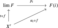
  Indeed, we have $\underline {p_{i} \circ t} \circ f \stackrel {(3.81)}{=} \alpha _{i} \circ f$ for all $i \in {\mathrm {Ob}}\, I$ and this shows that (3.80) holds.

  Consider now two functors F, $F^{\prime } \colon I \to \mathcal {C}$ and $\beta \in {\mathrm {Hom}}_{{\mathrm {Fun}}(I,\, \mathcal {C})}(F,\, F^{\prime })$, i.e., $\beta \colon F \to F^{\prime }$ is a natural transformation. We denote by $\big ({\mathrm {lim}}\, F,\, (p_{i} \colon {\mathrm {lim}}\, F \to F(i))_{i \in {\mathrm {Ob}}\, I}\big )$ and $\big ({\mathrm {lim}}\, F^{\prime },\, (s_{i} \colon {\mathrm {lim}}\, F^{\prime } \to F^{\prime }(i))_{i \in {\mathrm {Ob}}\, I}\big )$ the limit of F and $F^{\prime }$ respectively. The naturality of $\theta$ in the second variable comes down to proving the commutativity of the following diagram:

  
  $$\displaystyle \begin{aligned} {} {\mathrm{i.e}.,}\qquad {\mathtt{Hom}}_{\mathcal{C}}(X,\, \mathtt{lim}\, \beta) \circ \theta_{X,\, F} = \theta_{X,\, F^{\prime}} \circ {\mathtt{Hom}}_{{\mathrm{Fun}}(I,\, \mathcal{C})}(\varDelta(X),\, \beta). \end{aligned} $$

  (3.82)

  To this end, let $\gamma \in {\mathrm {Hom}}_{{\mathrm {Fun}}(I,\, \mathcal {C})}(\varDelta (X),\, F)$, i.e., $\alpha \colon \varDelta (X) \to F$ is a natural transformation. We obtain

  $$\displaystyle \begin{aligned} & {\mathtt{Hom}}_{\mathcal{C}}(X,\, \mathtt{lim}\, \beta) \circ \theta_{X,\, F} (\gamma) = \mathtt{lim}\, \beta \circ t, \\ &\theta_{X,\, F^{\prime}} \circ {\mathtt{Hom}}_{{\mathrm{Fun}}(I,\, \mathcal{C})}(\varDelta(X),\, \beta)(\gamma) = \theta_{X,\, F^{\prime}}\big(\beta \circ \gamma\big) = r, \end{aligned} $$

  where $t \colon X \to {\mathrm {lim}}\, F$ and $r \colon X \to {\mathrm {lim}}\, F^{\prime }$ are the unique morphisms in $\mathcal {C}$ which make the following diagrams commutative for all $i \in {\mathrm {Ob}}\, I$:

  

  (3.83)

  We are left to show that $\mathtt {lim}\, \beta \,\, \circ \, t = r$. To this end, recall that $\mathtt {lim}\, \beta \in {\mathrm {Hom}}_{\mathcal {C}}({\mathrm {lim}}\, F,\, {\mathrm {lim}}\, F^{\prime })$ is the unique morphism in $\mathcal {C}$ which makes the following diagram commute for all $i \in {\mathrm {Ob}}\, I$:

  

  (3.84)

  By Proposition 2.2.14, (1) we only need to show that $s_{i} \circ \mathtt {lim}\, \beta \circ t = s_{i} \circ r$ for all $i \in {\mathrm {Ob}}\, I$. Indeed, we have $\underline {s_{i} \circ \mathtt {lim}\, \beta } \circ t \stackrel {(3.84)}{=} \beta _{i} \circ \underline {p_{i} \circ t} \stackrel {(3.83)}{=} \underline {\beta _{i} \circ \gamma _{i}} \stackrel {(3.83)}{=} s_{i} \circ r$, as desired.

  Assume now that the diagonal functor $\varDelta \colon \mathcal {C} \to {\mathrm {Fun}}(I,\, \mathcal {C})$ has a right adjoint, denoted by $R \colon {\mathrm {Fun}}(I,\, \mathcal {C}) \to \mathcal {C}$. We will show that any functor $F \colon I \to \mathcal {C}$ has a limit. To this end, let $\varepsilon \colon \varDelta R \to 1_{{\mathrm {Fun}}(I,\, \mathcal {C})}$ and $\theta \colon {\mathtt {Hom}}_{{\mathrm {Fun}}(I,\, \mathcal {C})}(\varDelta ,\, -) \to {\mathtt {Hom}}_{\mathcal {C}}(-,\, R)$ be the counit and respectively the natural bijection induced by the adjunction $\varDelta \dashv R$. In particular, $\varepsilon _{F} \colon \varDelta _{R(F)} \to F$ is a natural transformation for any functor $F \colon I \to \mathcal {C}$. Proposition 2.2.4, (1) implies that $\big (R(F),\, (\varepsilon _{F})_{i}) \colon R(F) \to F(i)_{i \in {\mathrm {Ob}}\, I}\big )$ is a cone on F. We will show that $\big (R(F),\, (\varepsilon _{F})_{i}) \colon R(F) \to F(i)_{i \in {\mathrm {Ob}}\, I}\big )$ is in fact the limit of F. Indeed, consider another cone $\big (X,\, (\alpha _{i}) \colon X \to F(i)_{i \in {\mathrm {Ob}}\, I}\big )$ on F. Using again Proposition 2.2.4, (1) we obtain that $\alpha \colon \varDelta _{X} \to F$, where $\alpha = (\alpha _{i})_{i \in {\mathrm {Ob}}\, I}$, is a natural transformation, i.e., $\alpha \in {\mathrm {Hom}}_{{\mathrm {Fun}}(I,\, \mathcal {C})}(\varDelta _{X},\, F)$. Now Theorem 3.6.1, (3) yields a unique morphism $g \in {\mathrm {Hom}}_{\mathcal {C}}(X,\, R(F))$ such that the following diagram is commutative:

  

  (3.85)

  The above equality between the natural transformations $\varepsilon _{F} \circ \varDelta (g)$ and $\alpha$ comes down to identities between the corresponding morphisms associated to each $i \in {\mathrm {Ob}}\, I$. In light of Example 1.7.2, (5) we have $(\varepsilon _{F})_{i} \circ g = \alpha _{i}$ for all $i \in {\mathrm {Ob}}\, I$ and therefore the following diagram is commutative:

  

  The proof will be finished once we show that g is the unique morphism in $\mathcal {C}$ which makes the above diagram commutative. To this end, assume that $h \in {\mathrm {Hom}}_{\mathcal {C}}(X,\, R(F))$ such that $(\varepsilon _{F})_{i} \circ h = \alpha _{i}$ for all $i \in {\mathrm {Ob}}\, I$. This leads to $\varepsilon _{F} \circ \varDelta (h) = \alpha$ and the uniqueness of the morphism which makes diagram (3.85) commutative implies $g=h$, as desired.

□

Remark 3.10.2

Functors having a left adjoint which is also a right adjoint are called Frobenius functors in the literature (see [17] for further details). The notion was first introduced in [16] and is motivated by the following example coming from ring theory: a ring extension $R \to S$ is Frobenius (in the sense of [41]) if and only if the corresponding restriction of scalars functor (Example 1.5.3, (32)) is Frobenius. In light of Theorem 3.10.1, since for complete and cocomplete categories $\mathcal {C}$ the diagonal functor $\varDelta \colon \mathcal {C} \to {\mathrm {Fun}}(I,\, \mathcal {C})$ has both a left and a right adjoint, it is natural to ask when the two adjoints are naturally isomorphic (or, equivalently, when the diagonal functor is Frobenius). This problem was considered in [20] and, given a complete and cocomplete category $\mathcal {C}$, the small categories I for which the diagonal functor is Frobenius are characterized.$\square$

As a straightforward consequence of Theorem 3.10.1 we can easily conclude using Theorem 3.4.4 that if $\mathcal {C}$ is complete (resp. cocomplete) then the diagonal functor preserves colimits (resp. limits). However, we will see that even without the (co)completeness assumption on $\mathcal {C}$, the diagonal functor still preserves all existing small (co)limits.

Proposition 3.10.3

Let I be a small category and$\mathcal {C}$an arbitrary category. Then the diagonal functor$\varDelta \colon \mathcal {C} \to {\mathrm {Fun}}(I,\, \mathcal {C})$preserves all existing small (co)limits.

Proof

We only show that $\varDelta$ preserves limits; colimit preservation follows similarly and is left to the reader. To this end, let J be a small category and $G \colon J \to \mathcal {C}$ a functor whose limit we denote by $\big (L,\, (p_{j} \colon L \to G(j))_{j \in {\mathrm {Ob}}\, J}\big )$. First note that, as proved in Lemma 2.5.5, the pair $\Big (\varDelta (L),\, \big (\varDelta (p_{j}) \colon \varDelta (L) \to \varDelta (G(j))\big )_{j \in {\mathrm {Ob}}\, J}\Big )$ is a cone on $\varDelta \circ G \colon J \to {\mathrm {Fun}}(I,\, \mathcal {C})$. Recall that each natural transformation $\varDelta (p_{j})$ is defined by $\big ((\varDelta (p_{j})\big )_{i} = p_{j}$ for all $i \in {\mathrm {Ob}}\, I$.

Consider now another cone $\Big (U,\, \big (q_{j} \colon U \to \varDelta (G(j))\big )_{j \in {\mathrm {Ob}}\, J}\Big )$ on $\varDelta \circ G$, where $U \colon I \to \mathcal {C}$ is a functor and $q_{j}$ is a natural transformation for all $j \in {\mathrm {Ob}}\, J$. Hence, for all $u \in {\mathrm {Hom}}_{J}(j,\, t)$, the following diagram is commutative:

(3.86)

Therefore, for all $i \in {\mathrm {Ob}}\, I$ we have $\big (\varDelta (G(u))\big )_{i} \circ (q_{j})_{i} = (q_{t})_{i}$, which comes down to $G(u) \circ (q_{j})_{i} = (q_{t})_{i}$, i.e., the following diagram is commutative:

(3.87)

Note that the commutativity of (3.87) implies that

$$\displaystyle \begin{aligned} \Big(U(i),\, \big((q_{j})_{i} \colon U(i) \to G(j)\big)_{j \in {\mathrm{Ob}}\, J}\big) \end{aligned} $$

is a cone on G. Since $\big (L,\, (p_{j} \colon L \to G(j))_{j \in {\mathrm {Ob}}\, J}\big )$ is the limit of G, for any $i \in {\mathrm {Ob}}\, I$, there exists a unique $g_{i} \in {\mathrm {Hom}}_{\mathcal {C}}(U(i), L)$ such that the following diagram is commutative for all $j \in {\mathrm {Ob}}\, J$:

(3.88)

The proof will be finished once we show that $g = (g_{i})_{i \in {\mathrm {Ob}}\, I} \colon U \to \varDelta (L)$ is a natural transformation. To this end, let $v \in {\mathrm {Hom}}_{I}(i,\, s)$; we are left to prove the commutativity of the following diagram:

(3.89)

In light of Proposition 2.2.14, (1) it is enough to prove that for all $j \in {\mathrm {Ob}}\, J$ we have $p_{j} \circ g_{i} = p_{j} \circ g_{s} \circ U(v)$. Indeed, we have

$$\displaystyle \begin{aligned} \underline{p_{j} \circ g_{s}} \circ U(v)\, \stackrel{(3.88)}{=} \, \underline{(q_{j})_{s} \circ U(v)} \,=\, \underline{(q_{j})_{i}}\, \stackrel{(3.88)}{=} \,p_{j} \circ g_{i}, \end{aligned} $$

where the second equality holds because $q_{j} \colon U \to \varDelta (G(j))$ is a natural transformation. □

3.11 Freyd’s Adjoint Functor Theorem

Theorem 3.4.4 shows that right (left) adjoints preserve all existing small limits (colimits). However, in general, small limit/colimit preservation alone does not guarantee the existence of a left/right adjoint. Indeed, consider the unique functor $T \colon {\mathbf {Set}}(\subseteq ) \to \mathbf {1}$, where $\mathbf {1}$ is the discrete category with one object and ${\mathbf {Set}}(\subseteq )$ is the category defined in Example 1.2.2, (2). Note that the category ${\mathbf {Set}}(\subseteq )$ is cocomplete by Example 2.2.11 and does not posses a final object as shown in Example 1.3.10, (6). Therefore, T does not admit a right adjoint as can easily be seen from Example 3.4.1, (5) while it trivially preserves small colimits.

In this section we will prove that limit/colimit preservation is part of a necessary and sufficient condition which needs to be fulfilled by a functor in order to admit a left/right adjoint. Let $G\colon \mathcal {D} \to \mathcal {C}$ be a functor, $X \in {\mathrm {Ob}}\, \mathcal {C}$ and let $(X \downarrow G)$ be the comma category defined in Corollary 1.8.6, (1). We have an obvious forgetful functor $U\colon (X \downarrow G) \to \mathcal {D}$ defined for any $(f,\,Y) \in {\mathrm {Ob}}\big (X \downarrow G\big )$ and any morphism h in $(X \downarrow G)$ as follows:

$$\displaystyle \begin{aligned} U(f,\,Y) = Y,\,\,\,\,\, U(h) = h. \end{aligned} $$

Lemma 3.11.1

Let$G \colon \mathcal {D} \to \mathcal {C}$be a functor.

• (1) The functor G admits a left adjoint if and only if for all$X \in {\mathrm {Ob}}\, \mathcal {C}$the comma category$(X \downarrow G)$has an initial object.

• (2) The functor G admits a right adjoint if and only if for all$X \in {\mathrm {Ob}}\, \mathcal {C}$the comma category$(G \downarrow X)$has a final object.

Proof

• (1) Suppose first that G has a left adjoint $F\colon \mathcal {C} \to \mathcal {D}$ and let $\theta \colon {\mathtt {Hom}}_{\mathcal {D}}(F(-),\, -) \to {\mathtt {Hom}}_{\mathcal {C}}(-,\, G(-))$ be the natural isomorphism corresponding to the adjunction $F \dashv G$. Now consider $X \in {\mathrm {Ob}}\, \mathcal {C}$ and let $\eta \colon 1_{\mathcal {C}} \to GF$ be the unit of the adjunction. We will prove that $\big (\eta _{X},\, F(X)\big )$ is the initial object of the category $(X \downarrow G)$. Let $(v,\, W)$ be another object in $(X \downarrow G)$, i.e., $W \in {\mathrm {Ob}}\, \mathcal {D}$ and $v \in \mathrm {Hom}_{\mathcal {C}}(X,\, G(W))$. To this end, we need to find a unique morphism $f\colon \big (\eta _{X},\, F(X)\big ) \to (v,\, W)$ in $(X \downarrow G)$, i.e., a morphism $f \in {\mathrm {Hom}}_{\mathcal {D}}(F(X),\, W)$ such that the following diagram is commutative:

  

  (3.90)

  Recall from (the proof of) Theorem 3.5.1 that for all $u \in {\mathrm {Hom}}_{\mathcal {D}}(F(X),\, W)$ we have $G(u) \circ \eta _{X} = \theta _{X,\,W}(u)$. Now if we consider $f = \theta _{X,\,W}^{-1}(v)$ we obtain

  $$\displaystyle \begin{aligned} v = \theta_{X,\,W}(f) = G(f) \circ \eta_{X}, \end{aligned} $$

  as desired. The uniqueness of f with this property follows from the bijectivity of $\theta _{X,\,W}$.

  Conversely, assume now that for each $X \in {\mathrm {Ob}}\, \mathcal {C}$ the comma category $(X \downarrow G)$ has an initial object, which we denote by $(u_{X},\, V_{X})$, where $V_{X} \in {\mathrm {Ob}}\, \mathcal {D}$ and $u_{X} \in {\mathrm {Hom}}_{\mathcal {C}}(X,\, G(V_{X}))$. Hence, for any $(f,\,Y) \in {\mathrm {Ob}}\,(X \downarrow G)$ there exists a unique morphism $h\colon (u_{X},\, V_{X}) \to (f,\,Y)$ in $(X \downarrow G)$; in other words, for any $f \in \mathrm {Hom}_{\mathcal {C}}(X,\, G(Y))$ there exists a unique morphism $h \in {\mathrm {Hom}}_{\mathcal {D}}(V_{X},\, Y)$ making the following diagram commute:

  

  (3.91)

  We define a functor $F\colon \mathcal {C} \to \mathcal {D}$ on objects by $F(X) = V_{X}$ for all $X \in {\mathrm {Ob}}\, \mathcal {C}$. Consider now $f \in {\mathrm {Hom}}_{\mathcal {C}}(X,\, X^{\prime })$; then $u_{X^{\prime }} \circ f \in {\mathrm {Hom}}_{\mathcal {C}}(X,\, G(F(X^{\prime })))$ and, using (3.91), we define $F(f) \in {\mathrm {Hom}}_{\mathcal {D}}(F(X),\, F(X^{\prime }))$ to be the unique morphism such that

  $$\displaystyle \begin{aligned} {} GF(f) \circ u_{X} = u_{X^{\prime}} \circ f. \end{aligned} $$

  (3.92)

  Obviously $F(1_{X}) = 1_{F(X)}$ for all $X \in {\mathrm {Ob}}\, \mathcal {C}$ . Moreover, if $f \in {\mathrm {Hom}}_{\mathcal {C}}(X,\, X^{\prime })$ and $f^{\prime } \in {\mathrm {Hom}}_{\mathcal {C}}(X^{\prime },\, X^{\prime \prime })$ then $F(f^{\prime } \circ f)$ and $F(f^{\prime }) \circ F(f)$ are both morphisms in the comma category $(X \downarrow G)$ from $(u_{X},\, F(X))$ to $(u_{X^{\prime \prime }} \circ f^{\prime } \circ f,\, F(X^{\prime \prime }))$ so they must be equal as $(u_{X},\, F(X))$ is the initial object of $(X \downarrow G)$. Hence F is a functor and furthermore, according to (3.92), $u\colon 1_{\mathcal {C}} \to GF$ is a natural transformation. To summarize, we have constructed a natural transformation $u\colon 1_{\mathcal {C}} \to GF$ such that for any $f \in {\mathrm {Hom}}_{\mathcal {C}}(X,\, G(Y))$ there exists a unique $h \in {\mathrm {Hom}}_{\mathcal {D}}(F(X),\, Y)$ satisfying $G(h) \circ u_{X} = f$. Now Theorem 3.6.1, (2) implies that F is left adjoint to G, as desired.

• (2) Theorem 3.4.3 shows that $G \colon \mathcal {D} \to \mathcal {C}$ admits a right adjoint if and only if $G^{\mathit {op}} \colon \mathcal {D}^{\mathit {op}} \to \mathcal {C}^{\mathit {op}}$ admits a left adjoint. We have already proved in $1)$ that $G^{\mathit {op}}$ has a left adjoint if and only if for all $X \in {\mathrm {Ob}}\, \mathcal {C}^{\mathit {op}}$ the comma category $(X \downarrow G^{\mathit {op}})$ has an initial object. Furthermore, by Proposition 1.8.10 we have an isomorphism of categories between $(X \downarrow G^{\mathit {op}})^{\mathit {op}}$ and $(G \downarrow X)$. Now using Proposition 1.4.3, (2) we obtain that $(X \downarrow G^{\mathit {op}})$ has an initial object if and only if its opposite category, namely $(G \downarrow X)$, has a final object. By putting all the above together we obtain that G has a right adjoint if and only if for all $X \in {\mathrm {Ob}}\, \mathcal {C}$ the comma category $(G \downarrow X)$ has a final object.

□

Definition 3.11.2

Let $\mathcal {C}$ be a category.

• (1) A family $(K_{i})_{i \in I}$ of objects of $\mathcal {C}$, where I is a set, is called a weakly initial set if for any $C \in {\mathrm {Ob}}\, \mathcal {C}$ there exists a morphism $t^{j}_{C} \in {\mathrm {Hom}}_{\mathcal {C}}(K_{j},\, C)$ for some $j \in I$.

• (2) Dually, a family $(W_{i})_{i \in I}$ of objects of $\mathcal {C}$, where I is a set, is called a weakly final set if it is a weakly initial set in $\mathcal {C}^{\mathit {op}}$; that is, if for any $C \in {\mathrm {Ob}}\, \mathcal {C}$ there exists a morphism $l^{j}_{C} \in {\mathrm {Hom}}_{\mathcal {C}}(C,\, W_{j})$ for some $j \in I$.

Lemma 3.11.3

Let$\mathcal {C}$be a category. Then:

• (1) if$\mathcal {C}$is complete then$\mathcal {C}$has an initial object if and only if$\mathcal {C}$has a weakly initial set;

• (2) if$\mathcal {C}$is cocomplete then$\mathcal {C}$has a final object if and only if$\mathcal {C}$has a weakly final set.

Proof

• (1) Assume first that $\mathcal {C}$ has an initial object I; then $\{I\}$ is obviously a weakly initial set.

  Conversely, let $(K_{i})_{i \in I}$ be a weakly initial set. As $\mathcal {C}$ is complete and I is a set we can consider the product $\big (P,\, (\pi _{i}\colon P \to K_{i})_{i \in I}\big )$ of the family of objects $(K_{i})_{i \in I}$. Notice that for each $C \in {\mathrm {Ob}}\, \mathcal {C}$ there exists at least one morphism $u_{C} \in {\mathrm {Hom}}_{\mathcal {C}}(P,\, C)$ given by the composition for some $j~\in ~I$.

  Consider now the category J with ${\mathrm {Ob}}\, J = \{P\}$ and ${\mathrm {Hom}}_{J}(P,\,P) = {\mathrm {Hom}}_{\mathcal {C}}(P,\,P)$ and let $(L,\, q\colon L \to P)$ be the limit of the inclusion functor $F\colon J \to \mathcal {C}$.

  We will prove that L is the initial object of the category $\mathcal {C}$. Indeed, for any $C \in {\mathrm {Ob}}\, \mathcal {C}$ there exists at least one morphism in ${\mathrm {Hom}}_{\mathcal {C}}(L,\,C)$ given by the composition . Suppose now that we have two such morphisms f, $g \in {\mathrm {Hom}}_{\mathcal {C}}(L,\,C)$ and consider $(E,\, e\colon E \to L)$ to be the equalizer of $(f,\, g)$. Since $E \in {\mathrm {Ob}}\, \mathcal {C}$ there exists a morphism $u_{E} \in {\mathrm {Hom}}_{\mathcal {C}}(P,\,E)$ given by the composition for some $j \in I$. Thus $q\circ e\circ u_{E} \in {\mathrm {Hom}}_{\mathcal {C}}(P,\,P)$ and since $(L,\, q\colon L \to P)$ is in particular a cone on F, the following diagram is commutative:

  

  Thus we have $q\circ e\circ u_{E} \circ q = q = q \circ 1_{L}$ and by Proposition 2.2.14, (1) we get $e\circ u_{E} \circ q = 1_{L}$. This yields

  $$\displaystyle \begin{aligned} f = f \circ 1_{L} = f \circ e\circ u_{E} \circ q = g \circ e\circ u_{E} \circ q = g \circ 1_{L} = g,\end{aligned} $$

  where in the third equality we used the fact that $(E,\, e\colon E \to L)$ is the equalizer of $(f,\, g)$. We have obtained $f = g$ and hence L is an initial object of $\mathcal {C}$.

• (2) If $\mathcal {C}$ is cocomplete then $\mathcal {C}^{\mathit {op}}$ is complete and, as proved in 1), $\mathcal {C}^{\mathit {op}}$ has an initial object if and only if $\mathcal {C}^{\mathit {op}}$ has a weakly initial set. Equivalently, $\mathcal {C}$ has a final object if and only if $\mathcal {C}$ has a weakly final set.

□

We are now ready to state the main result of this section:

Theorem 3.11.4 (Freyd’s adjoint functor theorem)

Let$G\colon \mathcal {D} \to \mathcal {C}$be a functor.

• (1) If$\mathcal {D}$is a complete category then G has a left adjoint if and only if G preserves all small limits and for each$X \in {\mathrm {Ob}}\, \mathcal {C}$the comma category$(X \downarrow G)$has a weakly initial set.

• (2) If$\mathcal {D}$is a cocomplete category then G has a right adjoint if and only if G preserves all small colimits and for each$X \in {\mathrm {Ob}}\, \mathcal {C}$the comma category$(G \downarrow X)$has a weakly final set.

Proof

• (1) Suppose G has a left adjoint F. Then G is a right adjoint to F and by Theorem 3.4.4 it preserves limits. Moreover, by (the proof of) Lemma 3.11.1, (1) for any $X \in {\mathrm {Ob}}\, \mathcal {C}$, the pair $\big (\eta _{X},\, F(X)\big )$ is an initial object in $(X \downarrow G)$, where $\eta \colon 1_{\mathcal {C}} \to GF$ is the unit of the adjunction $(F,\,G)$.

  Assume now that $G\colon \mathcal {D} \to \mathcal {C}$ preserves small limits and for each $X \in {\mathrm {Ob}}\, \mathcal {C}$ the comma category $(X \downarrow G)$ has a weakly initial set. By Corollary 2.6.5, (1) the category $(X \downarrow G)$ is complete. Thus, from Lemma 3.11.3, (1) we obtain that $(X \downarrow G)$ has an initial object. The conclusion now follows by Lemma 3.11.1, (1).

• (2) The category $\mathcal {D}^{\mathit {op}}$ is complete and by applying (1) for the functor $G^{\mathit {op}} \colon \mathcal {D}^{\mathit {op}} \to \mathcal {C}^{\mathit {op}}$ it follows that $G^{\mathit {op}}$ has a left adjoint if and only if $G^{\mathit {op}}$ preserves small limits and for each $X \in {\mathrm {Ob}}\, \mathcal {C}$ the comma category $(X \downarrow G^{\mathit {op}})$ has a weakly initial set. Note also that by Theorem 3.4.3, G has a right adjoint if and only if $G^{\mathit {op}}$ has a left adjoint. Furthermore, Proposition 1.8.10 shows that the comma categories $(X \downarrow G^{\mathit {op}})$ and $(G \downarrow X)^{\mathit {op}}$ are isomorphic and therefore a weakly initial set in $(X \downarrow G^{\mathit {op}})$ is a weakly final set in $(G \downarrow X)$. Putting all of the above together we can conclude that G has a right adjoint if and only if G preserves all small colimits and for each $X \in {\mathrm {Ob}}\, \mathcal {C}$ the comma category $(G \downarrow X)$ has a weakly final set, as desired.

□

Theorem 3.11.4 can be stated in an equivalent form without the use of comma-categories. To this end, we introduce the following:

Definition 3.11.5

Let $F \colon \mathcal {C} \to \mathcal {D}$ be a functor and $D \in {\mathrm {Ob}}\, \mathcal {D}$. Then:

• (1) F satisfies the solution set condition with respect to D if there exists a set $U_{D}$ of objects of $\mathcal {C}$ such that for any $C \in {\mathrm {Ob}}\, \mathcal {C}$ and any $f \in {\mathrm {Hom}}_{\mathcal {D}}(D,\, F(C))$, there exists an object $C^{\prime } \in U_{D}$ and morphisms $u \in {\mathrm {Hom}}_{\mathcal {C}}(C^{\prime },\, C)$, $g \in {\mathrm {Hom}}_{\mathcal {D}}(D,\, F(C^{\prime }))$ such that the following diagram is commutative:

  

• (2) F satisfies the cosolution set condition with respect to D if there exists a set $W_{D}$ of objects of $\mathcal {C}$ such that for any $C \in {\mathrm {Ob}}\, \mathcal {C}$ and any $f \in {\mathrm {Hom}}_{\mathcal {D}}(F(C),\, D)$, there exists an object $C^{\prime } \in W_{D}$ and morphisms $u \in {\mathrm {Hom}}_{\mathcal {C}}(C,\, C^{\prime })$, $g \in {\mathrm {Hom}}_{\mathcal {D}}(F(C^{\prime }),\,D)$ such that the following diagram is commutative:

  

Example 3.11.6

If I is a small category and $\mathcal {C}$ is a cocomplete category then the diagonal functor $\varDelta \colon \mathcal {C} \to {\mathrm {Fun}}(I,\, \mathcal {C})$ satisfies the solution set condition with respect to all $G \in {\mathrm {Ob}}\big ({\mathrm {Fun}}(I,\, \mathcal {C})\big )$. Indeed, as $G \colon I \to \mathcal {C}$ is a functor and $\mathcal {C}$ is cocomplete, G has a colimit, which we denote as usual by $\big ({\mathrm {colim}}\, G,\, (q_{i} \colon G(i) \to {\mathrm {colim}}\, G)_{i \in {\mathrm {Ob}}\, I}\big )$. Consider now the set $U_{G} = \{{\mathrm {colim}}\, G\}$. If $C \in {\mathrm {Ob}}\, \mathcal {C}$ and $\alpha \in {\mathrm {Hom}}_{{\mathrm {Fun}}(I,\, \mathcal {C})}(G,\, \varDelta _{C})$ then by Proposition 2.2.4, (2) we obtain that $\big (C,\, (\alpha _{i} \colon G(i) \to C)_{i \in {\mathrm {Ob}}\, I}\big )$ is a cocone on G. As $\big ({\mathrm {colim}}\, G, (q_{i})_{i \in {\mathrm {Ob}}\, I}\big )$ is the colimit of G, there exists a unique $u \in {\mathrm {Hom}}_{\mathcal {C}}({\mathrm {colim}}\, G,\,C)$ such that for all $i \in {\mathrm {Ob}}\, I$ we have

$$\displaystyle \begin{aligned} {} u \circ q_{i} = \alpha_{i}. \end{aligned} $$

(3.93)

Furthermore, using again Proposition 2.2.4, (2) it follows that $\beta \colon G \to \varDelta _{{\mathrm {colim}}\, G}$ defined by $\beta _{i} = q_{i}$ for all $i \in {\mathrm {Ob}}\, I$ is a natural transformation and, moreover, (3.93) implies

$$\displaystyle \begin{aligned} {} \varDelta(u) \circ \beta = \alpha. \end{aligned} $$

(3.94)

To summarize, given $C \in {\mathrm {Ob}}\, \mathcal {C}$ and $\alpha \in {\mathrm {Hom}}_{{\mathrm {Fun}}(I,\, \mathcal {C})}(G,\, \varDelta _{C})$, there exists ${\mathrm {colim}}\, G \in U_{G}$ and two morphisms

$$\displaystyle \begin{aligned} u \in {\mathrm{Hom}}_{\mathcal{C}}({\mathrm{colim}}\, G,\,C), \qquad \beta \in {\mathrm{Hom}}_{{\mathrm{Fun}}(I,\, \mathcal{C})}(G,\, \varDelta_{{\mathrm{colim}}\, G}) \end{aligned} $$

such that (3.94) holds. This shows that $\varDelta \colon \mathcal {C} \to {\mathrm {Fun}}(I,\, \mathcal {C})$ satisfies the solution set condition with respect to all $G \in {\mathrm {Ob}}\big ({\mathrm {Fun}}(I,\, \mathcal {C})\big )$.

Similarly, it can be proved that if $\mathcal {C}$ is a complete category then the diagonal functor $\varDelta \colon \mathcal {C} \to {\mathrm {Fun}}(I,\, \mathcal {C})$ satisfies the cosolution set condition. $\square$

Theorem 3.11.7 (Freyd’s Adjoint Functor Theorem)

Let$G\colon \mathcal {D} \to \mathcal {C}$be a functor.

• (1) If$\mathcal {D}$is a complete category then G has a left adjoint if and only if G preserves all small limits and satisfies the solution set condition with respect to each$X \in {\mathrm {Ob}}\, \mathcal {C}$.

• (2) If$\mathcal {D}$is a cocomplete category then G has a right adjoint if and only if G preserves all small colimits and satisfies the cosolution set condition with respect to each$X \in {\mathrm {Ob}}\, \mathcal {C}$.

Proof

• (1) Note that G satisfies the solution set condition with respect to X if and only if the comma category $(X \downarrow G)$ has a weakly initial set and the conclusion follows by Theorem 3.11.4, (1). Indeed, assume first that G satisfies the solution set condition, let $X \in {\mathrm {Ob}}\, \mathcal {C}$ and let $U_{X}$ be the corresponding set as in Definition 3.11.5, (1). Then $\{(h,\, Y) ~|~ h \in {\mathrm {Hom}}_{\mathcal {C}}(X,\, G(Y)),\,\, Y \in U_{X}\}$ is a weakly initial set in $(X \downarrow G)$. Conversely, if $K = \{(t,\, Z) ~|~ Z \in {\mathrm {Ob}}\, \mathcal {D},\,\, t \in {\mathrm {Hom}_{\mathcal {C}}(\mathrm {X},\, \mathrm {G(Z)})\}}$ is a weakly initial set in $(X \downarrow G)$ then $U_{X} = \{D \in {\mathrm {Ob}}\, \mathcal {D} ~|~ {\mathrm {there} \,\, \mathrm {exists}\,\,}\,\, t \in {\mathrm {Hom}}_{\mathcal {C}}(X,\, G(Z)) \,\, {\mathrm {such}\,\, \mathrm {that}}\,\, (t,\, Z) \in K \}$ is a set which fulfills the condition in Definition 3.11.5, (1) and therefore G satisfies the solution set condition.

• (2) Similarly, G satisfies the cosolution set condition with respect to X if and only if the comma category $(G \downarrow X)$ has a weakly final set and Theorem 3.11.4, (2) leads to the desired conclusion.

□

We end this section with some applications of the adjoint functor theorem. As we will see, it can be used to show the existence of various free objects (such as free groups, free algebras, free modules etc.) without explicitly constructing them.

Examples 3.11.8

• (1) Let $U \colon {\mathbf {Grp}} \to {\mathbf {Set}}$ be the forgetful functor. We will show that U admits a left adjoint by using Freyd’s adjoint functor theorem. To start with, ${\mathbf {Grp}}$ is complete as shown in Example 2.4.3, (1) and U preserves small limits by Example 2.5.10, (1). In order to conclude that U admits a left adjoint we need to show that it satisfies the solution set condition with respect to each $X \in {\mathrm {Ob}}\, {\mathbf {Set}}$. To this end, for a given $X \in {\mathrm {Ob}}\, {\mathbf {Set}}$ we consider the class $\mathcal {U}_{X}$ of all isomorphism classes of groups of cardinality less than or equal to $\lambda =$ max$\{\aleph _{0},\, |X|\}$, where $\aleph _{0}$ denotes the cardinality of the set of all natural numbers. First we show that $\mathcal {U}_{X}$ is in fact a set. Indeed, recall that there is only a set of composition laws (in particular, of composition laws which are group structures) on any given set. Thus, we can conclude that we have, up to isomorphism, only a set of group structures on any set whose cardinality is at most $\lambda$. This shows that $\mathcal {U}_{X}$, being a reunion of sets, is a set itself.

  In order to show that $\mathcal {U}_{X}$ satisfies the conditions in Definition 3.11.5, (1) we start by proving that if $(g_{x})_{x \in X}$ is a set of elements of a group G then the subgroup $G_{X}$ of G generated by this set has cardinality at most $\lambda$. This can be easily seen by observing that the following map is surjective:

  $$\displaystyle \begin{aligned} f \colon\hspace{-1pt} \coprod_{n \in {\mathbb N}} \, (X \times {\mathbb Z})^{n}\hspace{-1pt} \to G_{X},\,\, f\big(\hspace{-0.5pt}(x_{1},\, e_{1}),\, (x_{2},\, e_{2}),\, \ldots\, (x_{n},\, e_{n})\hspace{-0.5pt}\big)\hspace{-1pt} = g_{x_{1}}^{e_{1}}g_{x_{2}}^{e_{2}} \ldots g_{x_{n}}^{e_{n}}, \end{aligned} $$

  where the domain of f is the coproduct of the family $\{(X \times {\mathbb Z})^{n}\}_{n \in {\mathbb N}}$ in Set. We have

  $$\displaystyle \begin{aligned} |G_{X}| &\leqslant \left|\coprod_{n \in {\mathbb N}} \, (X \times {\mathbb Z})^{n}\right| = \sum_{n \in {\mathbb N}} |(X \times {\mathbb Z})^{n}| \\ &= \left \{\begin{array}{rcl} \aleph_{0}, \, & \mbox{ if }& |X| \leqslant \aleph_{0} \\ |X|, \, & \mbox{ if }& |X| \gneqq \aleph_{0} \\ \end{array} \right. \leqslant {\mathrm{max}}\{\aleph_{0},\, |X|\} = \lambda. \end{aligned} $$

  Consider now $f \in {\mathrm {Hom}}_{{\mathbf {Set}}}(X,\, U(G))$ for some $G \in {\mathrm {Ob}}\, {\mathbf {Grp}}$ and let $G^{\prime }$ be the subgroup of G generated by the set $(f(x))_{x \in X}$. Then, according to the above discussion, $G^{\prime }$ is a group of cardinality at most $\lambda$ and we can find a group $H \in \mathcal {U}_{X}$ and a group isomorphism $t \colon H \to G^{\prime }$. Denote by $i \colon G^{\prime } \to G$ the inclusion map and consider $i \circ t \in {{\mathrm {Hom}}}_{\mathbf {Grp}}(H,\, G)$ and $U(t^{-1}) \circ f \in {{\mathrm {Hom}}}_{\mathbf {Set}}(X,\, U(H))$ such that the following diagram is commutative:

  

  We can now conclude by Freyd’s adjoint functor theorem that $U \colon {\mathbf {Grp}} \to {\mathbf {Set}}$ has a left adjoint.

• (2) Let R be a ring, $M \in {\mathrm {Ob}}\,\mathcal {M}_{R}$, $N \in {\mathrm {Ob}}\,{ }_{R}\mathcal {M}$ and ${\mathtt {Bil}}_{M,\,N} \colon {\mathbf {Ab}} \to {\mathbf {Ab}}$ the functor defined in Example 1.5.3, (28). We will show, using Freyd’s adjoint functor theorem, that ${\mathtt {Bil}}_{M,\,N}$ admits a left adjoint. By Example 2.5.4, ${\mathtt {Bil}}_{M,\,N}$ preserves limits. We are left to show that ${\mathtt {Bil}}_{M,\,N}$ satisfies the solution set condition for each $A \in {\mathrm {Ob}}\,{\mathbf {Ab}}$. To this end, for a given $A \in {\mathrm {Ob}}\,{\mathbf {Ab}}$ we denote by $\mathcal {U}_{A}$ the class of all isomorphism classes of abelian groups of cardinality less than or equal to $\lambda =$ max$\{\aleph _{0},\, |A|\cdot |M \times N|\}$. It follows easily, as in the previous example, that $\mathcal {U}_{A}$ is in fact a set.

  We will show that $\mathcal {U}_{A}$ satisfies the conditions in Definition 3.11.5, (1). Indeed, let $B \in {\mathrm {Ob}}\,{\mathbf {Ab}}$ and $f \in {\mathrm {Hom}}_{{\mathbf {Ab}}}(A,\, {\mathtt {Bil}}_{M,\,N}(B))$. For all $a \in A$ let $P_{a} = \{f(a)(m,\,n) ~|~ m \in M, \, n \in N\}$ and let $B^{\prime }$ be the abelian subgroup of B generated by the set $P = \cup _{a \in A} P_{a}$. We start by proving that $B^{\prime }$ has cardinality at most $\lambda$. This can be easily seen by observing that the following map is surjective:

  $$\displaystyle \begin{aligned} f \colon \coprod_{n \in {\mathbb N}} \, (P \times {\mathbb Z})^{n} \to B^{\prime},\,\,\, f\big((x_{1},\, k_{1}),\, (x_{2},\, k_{2}),\, \ldots\, (x_{n},\, k_{n})\big) = \sum_{i=1}^{n}\, k_{i} x_{i}, \end{aligned} $$

  where the domain of f is the coproduct of the family $\{(P \times {\mathbb Z})^{n}\}_{n \in {\mathbb N}}$ in Set. We have

  $$\displaystyle \begin{aligned} |B^{\prime}| &\leqslant \left|\coprod_{n \in {\mathbb N}} \, (P \times {\mathbb Z})^{n}\right| = \left|\coprod_{n \in {\mathbb N}} \, \big((\cup_{a \in A} P_{a}) \times {\mathbb Z}\big)^{n}\right| \\ &\leqslant \left \{\begin{array}{rl} \aleph_{0}, \, & \mbox{ if } |A|\cdot |M \times N| \leqslant \aleph_{0} \\ |A|\cdot |M \times N|, \, & \mbox{ if } |A|\cdot |M \times N| \gneqq \aleph_{0} \\ \end{array} \right.\\ &\leqslant {\mathrm{max}}\{\aleph_{0},\, |A|\cdot|M \times N|\} = \lambda. \end{aligned} $$

  Hence, there exists an abelian group $H \in \mathcal {U}_{A}$ and a group isomorphism $t \colon H \to B^{\prime }$. Now given the way we defined $B^{\prime }$, we obviously have $f \in {\mathrm {Hom}}_{{\mathbf {Ab}}}(A,\, {\mathtt {Bil}}_{M,\,N}(B^{\prime }))$. Summarizing, if we denote by $i \colon B' \to B$ the inclusion map, we have found two maps $i\, \circ \, t \in {{\mathrm {Hom}}}_{\mathbf {Ab}}(H,\, B)$ and ${\mathtt {Bil}}_{M,\,N}(t^{-1}) \circ f \in {{\mathrm {Hom}}}_{\mathbf {Ab}}(A,\, {\mathtt {Bil}}_{M,\,N}(H))$ such that the following diagram is commutative:

  

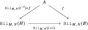
  Now Freyd’s adjoint functor theorem implies that ${\mathtt {Bil}}_{M,\,N} \colon {\mathbf {Ab}} \to {\mathbf {Ab}}$ has a left adjoint.

• (3) Let I be a small category and $\varDelta \colon {\mathbf {Grp}} \to {\mathrm {Fun}}(I,\, {\mathbf {Grp}})$ the diagonal functor. We show that $\varDelta$ admits a left adjoint by using Freyd’s adjoint functor theorem. To start with, ${\mathbf {Grp}}$ is a complete category by Example 2.4.3, (1) and the diagonal functor preserves limits as shown in Proposition 3.10.3. We are left to show that $\varDelta$ also fulfills the solution set condition. To this end, let $F \colon I \to {\mathbf {Grp}}$ be a functor and let $X_{i} = F(i)$, for all $i \in {\mathrm {Ob}}\,I$. Consider $\lambda = |\coprod _{i \in {\mathrm {Ob}}\, I} \, X_{j} |$ and let $U_{F}$ be the class of isomorphism classes of groups of cardinality less than or equal to $\lambda$, where $\coprod _{i \in {\mathrm {Ob}}\, I} \, X_{j}$ is the coproduct in Set of the underlying sets of the family of groups $(X_{i})_{i \in I}$. As in the first example, $U_{F}$ can be easily proved to be a set. Now let $C \in {\mathrm {Ob}}\,{\mathbf {Grp}}$ and $\psi \colon F \to \varDelta _{C}$ be a natural transformation. Consider H to be the subgroup of C generated by $\bigcup _{j \in {\mathrm {Ob}}\, I} \, \psi _{j}(X_{j})$, where $\psi _{j} \colon X_{j} \to C$, $j \in {\mathrm {Ob}}\, I$, are the group morphisms corresponding to the natural transformation $\psi$. In particular, we have $\psi \colon F \to \varDelta _{H}$. Furthermore, the following holds:

  $$\displaystyle \begin{aligned} |H| \leqslant |\bigcup_{j \in {\mathrm{Ob}}\, I} \, \psi_{j}(X_{j})| \leqslant |\coprod_{i \in {\mathrm{Ob}}\, I} \, X_{j} | = \lambda. \end{aligned} $$

  Therefore we can find a group $G_{\alpha } \in U_{F}$ and a group isomorphism $u \colon H \to G_{\alpha }$. Consider now the natural transformation $\tau \colon F \to \varDelta _{G_{\alpha }}$ defined for all $i \in {\mathrm {Ob}}\, I$ by $\tau _{i}(x) = u\big (\psi _{i}(x)\big )$, $x \in X_{i}$. It can be easily seen that $\tau$ is a natural transformation; indeed, if $v \in {\mathrm {Hom}}_{I}(i,\,j)$ and $x \in X_{i}$ we have

  $$\displaystyle \begin{aligned} \big(\tau_{j} \circ F(h)\big)(x) = u\big(\psi_{j}(F(h)(x))\big) = u \big(\psi_{i}(x)\big) = \tau_{i}(x), \end{aligned} $$

  where the second equality holds because $\psi$ is a natural transformation. Now define $t \colon G_{\alpha } \to C$ by $t(y) = u^{-1}(y)$ for all $y \in G_{\alpha }$. Note that for all $x \in X_{i}$ we have

  $$\displaystyle \begin{aligned} (t \circ \tau_{i})(x) = t \big(u(\psi_{i}(x))\big) = u^{-1}\big(u(\psi_{i}(x))\big) = \psi_{i}(x). \end{aligned} $$

  This shows that the following diagram is commutative:

  

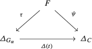
  and therefore $U_{F}$ is indeed a solution set. We can now conclude by Freyd’s adjoint functor theorem that $\varDelta$ has a left adjoint. Furthermore, we can derive the cocompleteness of ${\mathbf {Grp}}$ from Theorem 3.10.1, (2).$\square$

3.12 Special Adjoint Functor Theorem

In this section we show that under certain conditions on the domain category, a given functor admits a left (right) adjoint if and only if it preserves small limits (colimits). We start with some preparations.

Definition 3.12.1

Let $\mathcal {C}$ be a category.

• (1) We say that $\mathcal {C}$ admits a set of generators (or separators) if there exists a set of objects $\{S_{i} \,|\, i \in I\}$ in $\mathcal {C}$ with the property that for any two morphisms u, $v \in {\mathrm {Hom}}_{\mathcal {C}}(A,\,B)$ such that $u \neq v$ there exists a morphism $g \in {\mathrm {Hom}}_{\mathcal {C}}(S_{j},\,A)$, for some $j \in I$, satisfying $u \circ g \neq v \circ g$. An object S of $\mathcal {C}$ is called a generator (or separator) if $\{S\}$ is a set of generators.

• (2) Dually, we say that $\mathcal {C}$ admits a set of cogenerators (or coseparators) if $\mathcal {C}^{\mathit {op}}$ admits a set of separators. More precisely, $\mathcal {C}$ admits a set of cogenerators if there exists a set of objects $\{U_{i} \,|\, i \in I\}$ in $\mathcal {C}$ with the property that for any two morphisms u, $v \in {\mathrm {Hom}}_{\mathcal {C}}(A,\,B)$ such that $u \neq v$ there exists a morphism $h \in {\mathrm {Hom}}_{\mathcal {C}}(B,\, U_{j})$, for some $j \in I$, satisfying $h \circ u \neq h \circ v$. An object U of $\mathcal {C}$ is called a cogenerator (or coseparator) if $\{U\}$ is a set of cogenerators.

Examples 3.12.2

• (1) In Set, any set with only one element is a generator while any set with at least two elements set is a cogenerator. Indeed, let u, $v \colon X \to Y$ be two functions such that $u \neq v$. Hence there exists an $x_{0} \in X$ such that $u(x_{0}) \neq v(x_{0})$ and we can define a map $g \colon \{\star \} \to X$ by $g(\star ) = x_{0}$. Therefore, we have a map g such that $u(g(\star )) = u(x_{0}) \neq v(x_{0}) = v(g(\star ))$. This shows that $u \circ g \neq v \circ g$ and the singleton $\{\star \}$ is a generator in Set. Similarly, one can show that any singleton set is a generator in Top.

  Next we look at cogenerators in Set. With the notations above, let $u(x_{0}) = y^{\prime }$ and $v(x_{0}) = y^{\prime \prime }$ where y, $y^{\prime } \in Y$ and $y^{\prime } \neq y^{\prime \prime }$. We can now define a map $h \colon Y \to Z$ by

  $$\displaystyle \begin{aligned} h(y) = \left\{ \begin{array}{rcl} z^{\prime}, & \mbox{if}& y = y^{\prime},\\ z^{\prime\prime}, & \mbox{if}& y \neq y^{\prime}, \end{array}\right. \end{aligned} $$

  where Z is a set with at least two elements and $z^{\prime } \neq z^{\prime \prime }$. This leads to $h(u(x_{0})) = h(y^{\prime }) = z^{\prime } \neq z^{\prime \prime } = h(y^{\prime \prime }) = h(v(x_{0}))$ and the desired conclusion follows.

• (2) In Grp, the group of integers $\big ({\mathbb Z},\, +\big )$ is a generator. To this end, let u, $v \in {\mathrm {Hom}}_{{\mathbf {Grp}}}(G,\,H)$ such that $u \neq v$ and consider $g_{0} \in G$ such that $u(g_{0}) \neq v(g_{0})$. Now define $g \colon {\mathbb Z} \to G$ by $g(k) = g_{0}^{k}$ for all $k \in {\mathbb Z}$, where the group structure on G is considered to be multiplicative. It can be easily seen that g is a morphism of groups and moreover $u(g(1)) \neq v(g(1))$, which leads to $u \circ g \neq v \circ g$, as desired.

  On the other hand, Grp has no cogenerators. To this end, assume there exists a cogenerator U in Grp and let S be a simple group whose cardinality is larger than that of U.¹² Let ${\mathrm {Id}}_{S}$, $0_{S} \in {\mathrm {Hom}}_{{\mathbf {Grp}}}(S,\,S)$, where ${\mathrm {Id}}_{S}$ denotes the identity morphism on S while $0_{S}$ is defined by $0_{S}(s) = 1_{S}$ for all $s \in S$. As S is a simple group we have ${\mathrm {Id}}_{S} \neq 0_{S}$ and since U is assumed to be a cogenerator in Grp, we have a group homomorphism $f \colon S \to U$ such that:

  $$\displaystyle \begin{aligned} {} f \circ {\mathrm{Id}}_{S} \neq f \circ 0_{S}. \end{aligned} $$

  (3.95)

  Now ${\mathrm {ker}}(f) \unlhd S$ and since S is a simple group we have either ${\mathrm {ker}}(f) = S$ or ${\mathrm {ker}}(f) = \{1_{S}\}$. The first option is ruled out by (3.95) and therefore we obtain ${\mathrm {ker}}(f) = \{1_{S}\}$. This shows that f is injective, which implies that the cardinality of S is less than or equal to the cardinality of U, contradicting our hypothesis. Therefore, we have reached a contradiction and we can conclude that Grp has no cogenerators.

• (3) In KHaus, the category of compact Hausdorff spaces, the unit interval $[0,\,1]$ is a cogenerator. Indeed, consider u, $v \in {\mathrm {Hom}}_{{\mathbf {KHaus}}}(H,\,K)$ such that $u \neq v$. Then, there exists an $h_{0} \in h$ such that $u(h_{0}) \neq v(h_{0})$. As K is in particular a Hausdorff space, there exist two disjoint neighborhoods $U_{0}$ and $V_{0}$ of $u(h_{0})$ and $v(h_{0})$, respectively. Now since any compact Hausdorff space is normal¹³ ([39, Theorem 32.3]), we can apply Urysohn’s lemma¹⁴ to conclude that there exists a continuous map $f \colon K \to [0,\,1]$ such that $f(x) = 0$ for all $x \in U_{0}$ and $f(x) = 1$ for all $x \in V_{0}$. In particular, we have $f\big (u(h_{0})\big ) = 0$ and $f\big (v(h_{0})\big ) = 1$, which shows that there exists an $f \in {\mathrm {Hom}}_{{\mathbf {KHaus}}}(K,\, [0,\,1])$ such that $f \circ u \neq f \circ v$. This shows that $[0,\,1]$ is a cogenerator in KHaus.

• (4) If J is a small category, then the functor category ${\mathrm {Fun}}(J,\, {\mathbf {Set}})$ has a set of generators. Indeed, we will show that $\{{\mathrm {Hom}}_{J}(j,\,-) ~|~ j \in {\mathrm {Ob}}\, J\}$ is a set of generators. To this end, let F, $G \in {\mathrm {Ob}}\, {\mathrm {Fun}}(J,\, {\mathbf {Set}})$, i.e., F and G are functors, and consider two natural transformations $\alpha$, $\beta \colon F \to G$ such that $\alpha \neq \beta$. Since $\alpha \neq \beta$, there exists $j_{0} \in {\mathrm {Ob}}\, J$ and some $x_{0} \in F(j_{0})$ such that $\alpha _{j_{0}}(x_{0}) \neq \beta _{j_{0}}(x_{0})$. Consider now $h^{x_{0}} \colon {\mathrm {Hom}}_{J}(j_{0},\,-) \to F$ defined for all $k \in {\mathrm {Ob}}\, J$ and $f \in {\mathrm {Hom}}_{J}(j_{0},\,k)$ by $\big (h^{x_{0}}\big )_{k}(f) = F(f)(x_{0})$. According to (the proof of) Yoneda’s lemma we have $h^{x_{0}} \in {\mathrm {Nat}}\big ({\mathrm {Hom}}_{J}(j_{0},\,-),\, F\big )$ and, consequently $\alpha \circ h^{x_{0}}$, $\beta \circ h^{x_{0}} \in {\mathrm {Nat}}\big ({\mathrm {Hom}}_{J}(j_{0},\,-),\, G\big )$. Furthermore, we have

  $$\displaystyle \begin{aligned} \big(\alpha \circ h^{x_{0}}\big)_{j_{0}}(1_{j_{0}}) &= \alpha_{j_{0}} \circ (h^{x_{0}})_{j_{0}}(1_{j_{0}}) = \alpha_{j_{0}}\big(F(1_{j_{0}})(x_{0})\big)\\ &= \alpha_{j_{0}}\big(1_{F(j_{0})}(x_{0})\big) = \alpha_{j_{0}}(x_{0}). \end{aligned} $$

  A similar computation shows that $\big (\beta \circ h^{x_{0}}\big )_{j_{0}}(1_{j_{0}}) = \beta _{j_{0}}(x_{0})$. As $\alpha _{j_{0}}(x_{0}) \neq \beta _{j_{0}}(x_{0})$ we obtain $\big (\alpha \circ h^{x_{0}}\big )_{j_{0}}(1_{j_{0}}) \neq \big (\beta \circ h^{x_{0}}\big )_{j_{0}}(1_{j_{0}})$. Therefore, $\alpha \circ h^{x_{0}} \neq \beta \circ h^{x_{0}}$, as desired. $\square$

Proposition 3.12.3

Let$S = \{X_{i} \,|\, i \in I\}$be a set of objects of a category$\mathcal {C}$.

• (1) Assume$\mathcal {C}$has products, S is a set of cogenerators and consider the product$\big (P,\, (p_{f})_{f \in {\mathrm {Hom}}_{\mathcal {C}}(C,\,X_{i})} \big )$of the family S, where the product consists of as many copies of$X_{i}$as there are morphisms in${\mathrm {Hom}}_{\mathcal {C}}(C,\,X_{i})$. Then, for any$C \in {\mathrm {Ob}}\,\mathcal {C}$, the unique morphism$\gamma _{C} \colon C \to P$which makes the following diagram commutative for all$i \in I$and all$f \in {\mathrm {Hom}}_{\mathcal {C}}(C,\,X_{i})$:

  

  (3.96)

  is a monomorphism.

• (2) Dually, assume$\mathcal {C}$has coproducts, S is a set of generators and consider the coproduct$\big (Q,\, (q_{f})_{f \in {\mathrm {Hom}}_{\mathcal {C}}(X_{i},\,C)} \big )$of the family S, where the coproduct consists of as many copies of$X_{i}$as there are morphisms in${\mathrm {Hom}}_{\mathcal {C}}(X_{i},\,C)$. Then, for any$C \in {\mathrm {Ob}}\,\mathcal {C}$, the unique morphism$\xi _{C} \colon P \to C$which makes the following diagram commutative for all$i \in I$and all$f \in {\mathrm {Hom}}_{\mathcal {C}}(X_{i},\,C)$:

  

  (3.97)

  is an epimorphism.

Proof

• (1) Consider u, $v \in {\mathrm {Hom}}_{\mathcal {C}}(A,\,C)$ such that $\gamma _{C}\, \circ \, u = \gamma _{C}\, \circ \, v$. This implies $p_{f}\, \circ \, \gamma _{C} \,\circ \, u = p_{f} \,\circ \, \gamma _{C}\, \circ \,v$ for all $i \in I$ and all $f \in {\mathrm {Hom}}_{\mathcal {C}}(C,\,X_{i})$. The commutativity of (3.96) leads to $f \circ u = f \circ v$ for all $i \in I$ and all $f \in {\mathrm {Hom}}_{\mathcal {C}}(C,\,X_{i})$. As S is a set of cogenerators we obtain $u = v$, as desired.

• (2) Consider u, $v \in {\mathrm {Hom}}_{\mathcal {C}}(C,\, D)$ such that $u \,\circ \, \xi _{C} = v\, \circ \, \xi _{C}$. This implies $u \,\circ \, \xi _{C} \,\circ \, q_{f} = v \,\circ \, \xi _{C} \, \circ \, q_{f}$ for all $i \in I$ and all $f \in {\mathrm {Hom}}_{\mathcal {C}}(X_{i},\,C)$. The commutativity of (3.97) leads to $u \circ f = v \circ f$ for all $i \in I$ and all $f \in {\mathrm {Hom}}_{\mathcal {C}}(X_{i},\, C)$. As S is a set of generators we obtain $u = v$, as desired.

□

Having introduced the necessary concepts, we can now state the main result of this section.

Theorem 3.12.4 (Special Adjoint Functor Theorem)

Let$F \colon \mathcal {C} \to \mathcal {D}$be a functor.

• (1) Assume$\mathcal {C}$is a complete, well-powered category which admits a cogenerating set. Then F admits a left adjoint if and only if F preserves small limits.

• (2) Assume$\mathcal {C}$is a cocomplete, co-well-powered category which admits a generating set. Then F admits a right adjoint if and only if F preserves small colimits.

Proof

• (1) If F admits a left adjoint then F is a right adjoint and it preserves limits by Theorem 3.4.4.

  Assume now that F preserves small limits and consider $D \in {\mathrm {Ob}}\, \mathcal {D}$. In light of Theorem 3.11.7, (1) it suffices to find a solution set for D. To this end, consider a coseparating set $S = \{G_{i} \,|\, i \in I\}$ of $\mathcal {C}$ and denote by

  $$\displaystyle \begin{aligned} \Big(P,\, \big(p_{f}\big)_{{\begin{subarray}{l} i \in I\\ f \in {\mathrm{Hom}}_{\mathcal{C}}(C,\,G_{i}) \end{subarray}}} \Big) \end{aligned} $$

  the product of the family S, where the product consists of as many copies of $G_{i}$ as there are elements in ${\mathrm {Hom}}_{\mathcal {C}}(C,\,G_{i})$, where C is a fixed object. Similarly, we consider the product

  $$\displaystyle \begin{aligned} \Big(P^{\prime},\, \big(q_{f}\big)_{{\begin{subarray}{l} i \in I\\ f \in {\mathrm{Hom}}_{\mathcal{D}}(D,\,F(G_{i})) \end{subarray}}} \Big) \end{aligned} $$

  of the same family S, but this time consisting of as many copies of $G_{i}$ as there are morphisms in ${\mathrm {Hom}}_{\mathcal {D}}(D,\,F(G_{i}))$.

  Let $U_{D} = \{ T \,|\, T \,\, {\mathrm {is}}\,\, {\mathrm {a}}\,\, {\mathrm {subobject}}\,\, {\mathrm {of}}\,\, P^{\prime }\}$. Note that $U_{D}$ is in fact a set as $\mathcal {C}$ is well-powered.

  Consider now $g \in {\mathrm {Hom}}_{\mathcal {D}}(D,\,F(C))$. By Proposition 3.12.3, (1) the unique morphism $\alpha _{C} \in {{\mathrm {Hom}}}_{\mathcal {C}}(C,\, P)$ such that the following holds for all $i \in I$ and all $f \in {\mathrm {Hom}}_{\mathcal {C}}(C,\,G_{i})$

  

  (3.98)

  is a monomorphism.

  As $\Big (P,\, \big (p_{f}\big )_{{\begin {subarray}{l} i \in I\\ f \in {\mathrm {Hom}}_{\mathcal {C}}(C,\,G_{i}) \end {subarray}}} \Big )$ is a product, there exists a unique morphism $\beta _{C} \colon P^{\prime } \to P$ such that the following diagram is commutative for all $i \in I$ and all $f \in {\mathrm {Hom}}_{\mathcal {C}}(C,\,G_{i})$:

  

  (3.99)

  As $\mathcal {C}$ is a complete category, the pair of morphisms $(\alpha _{C},\,\beta _{C})$ admits a pullback, which we denote by $(S,\, \mu ,\,\gamma )$

  

  (3.100)

  Furthermore, since $\alpha _{C}$ is a monomorphism it follows by Proposition 2.1.17, (1) that $\gamma$ is also a monomorphism and therefore we can assume without loss of generality that $S \in U_{D}$. Indeed, if $S \notin U_{D}$, then there exists some $S^{\prime } \in U_{D}$ together with a monomorphism $\gamma ^{\prime } \colon S^{\prime } \to P^{\prime }$ and an isomorphism $u \in {\mathrm {Hom}}_{\mathcal {C}}(S^{\prime },\, S)$ such that $\gamma ^{\prime } = \gamma \circ u$. Then, the triple $(S^{\prime },\, \gamma \circ u,\, \mu \circ u)$ is also a pullback of the pair of morphisms $(\alpha _{C},\,\beta _{C})$ and $S^{\prime } \in U_{D}$.

  As F is assumed to be limit preserving, $\Big (F(P^{\prime }),\, \big (F(q_{f})\big )_{{\begin {subarray}{l} i \in I\\ f \in {\mathrm {Hom}}_{\mathcal {D}}(D,\,F(G_{i})) \end {subarray}}}\Big )$ is the product of the family $\{F(G_{i}) \,|\, i \in I\}$, where the product consists of as many copies of $G_{i}$ as there are morphisms in ${\mathrm {Hom}}_{\mathcal {D}}(D,\,F(G_{i}))$. Hence, we obtain a unique morphism $\lambda \colon D \to F(P^{\prime })$ such that the following diagram is commutative for all $i \in I$ and all $h \in {\mathrm {Hom}}_{\mathcal {D}}(D,\,F(G_{i}))$:

  

  (3.101)

  Now using again the fact that F is limit preserving we obtain, in particular, that $\Big (F(P),\, \big (F(p_{f})\big )_{{\begin {subarray}{l} i \in I\\ f \in {\mathrm {Hom}}_{\mathcal {C}}(C,\,G_{i}) \end {subarray}}}\Big )$ is the product of the family $\{F(G_{i}) \,|\, i \in I\}$, where the product consists of as many copies of $G_{i}$ as there are morphisms in ${\mathrm {Hom}}_{\mathcal {C}}(C,\,G_{i})$. Therefore, for all $i \in I$ and all $f \in {\mathrm {Hom}}_{\mathcal {C}}(C,\,G_{i})$ we have

  $$\displaystyle \begin{aligned} &F(p_{f}) \circ F(\alpha_{C}) \circ g = F(\underline{p_{f} \circ \alpha_{C}}) \circ g \stackrel{(3.98)}{=} \underline{F(f) \circ g} \stackrel{(3.101)}{=} F\big(\underline{q_{F(f) \circ g}}\big) \circ \lambda\\ &\stackrel{(3.99)}{=} F\big(p_{f} \circ \beta_{C}\big) \circ \lambda = F(p_{f}) \circ F(\beta_{C}\big) \circ \lambda. \end{aligned} $$

  Proposition 2.2.14, (1) implies that $F(\alpha _{C}) \circ g = F(\beta _{C}\big ) \circ \lambda$. As F is limit preserving it follows that $(F(S),\, F(\mu ),\,F(\gamma ))$ is the pullback of the pair of morphisms $(F(\alpha _{C}),\,F(\beta _{C}))$ and we obtain a unique morphism $g^{\prime } \in {\mathrm {Hom}}_{\mathcal {D}}(D,\, F(S))$ such that $F(\mu ) \circ g^{\prime } = g$ and $F(\gamma ) \circ g^{\prime } = \lambda$. The complete picture is captured in the diagram below:

  

  To conclude, we have proved that for any $C \in {\mathrm {Ob}}\, \mathcal {C}$ and $g \in {\mathrm {Hom}}_{\mathcal {D}}(D,\,F(C))$ there exists some $S \in U_{D}$ together with morphisms $\mu \in {\mathrm {Hom}}_{\mathcal {C}}(S,\, C)$ and $g^{\prime } \in {\mathrm {Hom}}_{\mathcal {D}}(D,\, F(S))$ such that $F(\mu ) \circ g^{\prime } = g$. The desired conclusion now follows by Theorem 3.11.7, (1).

• (2) To start with, note that the category $\mathcal {C}^{\mathit {op}}$ is complete, well-powered and admits a coseparating set. By applying $1)$ for the functor $F^{\mathit {op}} \colon \mathcal {C}^{\mathit {op}} \to \mathcal {D}^{\mathit {op}}$, we obtain that $F^{\mathit {op}}$ admits a left adjoint if and only if $F^{\mathit {op}}$ preserves small limits. In light of Lemma 2.5.2 and Theorem 3.4.3 it follows that F admits a right adjoint if and only if F preserves small colimits, as desired.

□

Corollary 3.12.5

Let$\mathcal {C}$be a category.

• (1) If$\mathcal {C}$is complete, well-powered and admits a coseparating set, then$\mathcal {C}$is also cocomplete.

• (2) If$\mathcal {C}$is cocomplete, co-well-powered and admits a separating set, then$\mathcal {C}$is also complete.

Proof

• (1) Consider the diagonal functor $\varDelta \colon \mathcal {C} \to {\mathrm {Fun}}(I,\, \mathcal {C})$ which preserves small limits, as proved in Proposition 3.10.3. Since the conditions in Theorem 3.12.4, (1) are fulfilled it follows that $\varDelta$ admits a left adjoint. Now Theorem 3.10.1, (2) implies that $\mathcal {C}$ is cocomplete.

• (2) The diagonal functor $\varDelta \colon \mathcal {C} \to {\mathrm {Fun}}(I,\, \mathcal {C})$ also preserves small colimits, as proved in Proposition 3.10.3. Since the conditions in Theorem 3.12.4, (2) are fulfilled it follows that $\varDelta$ admits a right adjoint. Now Theorem 3.10.1, (1) implies that $\mathcal {C}$ is complete.

□

Examples 3.12.6

• (1) Let $U \colon {\mathbf {KHaus}} \to {\mathbf {Top}}$ be the forgetful functor. Recall that KHaus, the category KHaus of compact Hausdorff spaces, is well-powered, as shown in Example 1.3.16, and has a cogenerator by Example 3.12.2, (3). Furthermore, KHaus has products (Example 2.1.5, (4)) and equalizers (Example 2.1.10, (4)), which shows that is complete by Theorem 2.4.2. As both products and equalizers are constructed as in Top we can conclude by the Special Adjoint Functor Theorem that U has a left adjoint.

• (2) Let $F \colon K \to J$ be a functor between small categories and consider the induced functor $F^{\star } \colon {\mathrm {Fun}}(J,\, {\mathbf {Set}}) \to {\mathrm {Fun}}(K,\, {\mathbf {Set}})$ defined in (1.37)

  $$\displaystyle \begin{aligned} F^{\star}(G) = GF,\,\,\, F^{\star}(\psi)_{k} = \psi_{F(k)} \end{aligned} $$

  for all functors G, $H \colon J \to {\mathbf {Set}}$ and all natural transformations $\psi \colon G \to H$. We will use the Special Adjoint Functor Theorem to prove that $F^{\star }$ has a right adjoint. Indeed, note that the category ${\mathrm {Fun}}(J,\, {\mathbf {Set}})$ has a set of generators, as proved in Example 3.12.2, (4). Furthermore, Set is cocomplete by Example 2.4.4 while Example 2.7.4 shows that ${\mathrm {Fun}}(J,\, {\mathbf {Set}})$ is also cocomplete. As Set is cocomplete, it follows from Proposition 2.7.5 that a morphism $\psi \colon F \to G$ in ${\mathrm {Fun}}(J,\, {\mathbf {Set}})$ (i.e., a natural transformation) is an epimorphism if and only if each $\psi _{j} \colon F(j) \to G(j)$ is an epimorphism in Set for all $j \in {\mathrm {Ob}}\, J$. Set is co-well-powered by Example 1.3.16, which shows that each $F(j)$ has only a set of quotients and since J is small we can conclude that F has a set of quotients. Therefore, ${\mathrm {Fun}}(J,\, {\mathbf {Set}})$ is co-well-powered. We are left to show that $F^{\star }$ preserves colimits. To this end, let $G \colon I \to {\mathrm {Fun}}(J,\, {\mathbf {Set}})$ and denote by $\big (H,\, (q_{i} \colon G(i) \to H)_{i \in {\mathrm {Ob}}\,I}\big )$ its colimit, where $H \colon J \to {\mathbf {Set}}$ is a functor and $q_{i}$ is a natural transformation for all $i \in {\mathrm {Ob}}\,I$. The proof will be finished once we show that $\Big (F^{\star }(H),\, \big (F^{\star }(q_{i})\big )_{i \in {\mathrm {Ob}}\, I}\Big )$ is the colimit of the functor $F^{\star } \circ G \colon I \to {\mathrm {Fun}}(K,\, {\mathbf {Set}})$. In light of Theorem 2.7.2 it is enough to prove that for any $k \in {\mathrm {Ob}}\, K$ the pair $\Big (F^{\star }(H)(k),\, \big (F^{\star }(q_{i})_{k}\big )_{i \in {\mathrm {Ob}}\, I}\Big )$ is the colimit of $(F^{\star } \circ G)_{k} \colon I \to {\mathbf {Set}}$, where $(F^{\star } \circ G)_{k}$ denotes the induced functor as defined in (2.40).

  We start by showing that $\Big (F^{\star }(H)(k),\, \big (F^{\star }(q_{i})_{k}\big )_{i \in {\mathrm {Ob}}\, I}\Big )$ is a cocone on $(F^{\star } \circ G)_{k} \colon I \to {\mathbf {Set}}$, i.e., for all $u \in {\mathrm {Hom}}_{I}(l,\,t)$ the following diagram is commutative:

  

  (3.102)

  Indeed, recall from Theorem 2.7.2 that $\big (H(j),\, (q^{j}_{i} \colon G_{j}(i) \to H(j))_{i \in {\mathrm {Ob}}\, I}\big )$ is the colimit of the induced functor $G_{j} \colon I \to {\mathbf {Set}}$ and in particular a cocone on $G_{j}$, where $q^{j}_{i} = (q_{i})_{j}$ for all $i \in {\mathrm {Ob}}\, I$ and $j \in {\mathrm {Ob}}\, J$. Therefore, the following diagram is commutative:

  

  (3.103)

  Now note that since we have

  $$\displaystyle \begin{aligned} &F^{\star}(H)(k) = H(F(k)),\\ &F^{\star}(q_{l})_{k} = (q_{l})_{F(k)} = q_{l}^{F(k)},\\ &(F^{\star} \circ G)_{k}(u) = \big((F^{\star} \circ G)(u)\big)_{k} = F^{\star}(G(u))_{k} = G(u)_{F(k)},\\ &(F^{\star} \circ G)_{k}(l) = (F^{\star} \circ G)(l)(k) = F^{\star}(G(l))(k) = G(l)(F(k)) = G_{F(k)}(l), \end{aligned} $$

  it can be easily seen that the commutativity of (3.103) implies the commutativity of (3.102).

  Consider now another cocone $\big (X_{k},\, (s_{i}^{k} \colon (F^{\star } \circ G)_{k}(i) \to X_{k})_{i \in {\mathrm {Ob}}\, I}\big )$ on the functor $(F^{\star } \circ G)_{k} \colon I \to {\mathbf {Set}}$. Hence, for all $u \in {\mathrm {Hom}}_{I}(l,\,t)$ the following diagram is commutative:

  

  As $(F^{\star } \circ G)_{k}(u) = G(u)_{F(k)}$ and $(F^{\star } \circ G)_{k}(i) = G_{F(k)}(i)$, the commutativity of the above diagram comes down to $G(u)_{F(k)} \circ s_{l}^{k} = s_{t}^{k}$. Therefore, $\big (X_{k},\, (s_{i}^{k} \colon G_{F(k)}(i) \to X_{k})_{i \in {\mathrm {Ob}}\, I}\big )$ is a cocone on the induced functor $G_{F(k)} \colon I \to {\mathbf {Set}}$. Now recall that the pair $\big (H(F(k)),\, (q^{F(k)}_{i} \colon G_{F(k)}(i) \to H(F(k)))_{i \in {\mathrm {Ob}}\, I}\big )$ is the colimit of the functor $G_{F(k)}$. Thus, we have a unique morphism $f \in {\mathrm {Hom}}_{{\mathbf {Set}}}(H(F(k)),\, X_{k})$ such that the following diagram is commutative for all $i \in {\mathrm {Ob}}\, I$:

  

  To conclude, there exists a unique morphism $f \in {\mathrm {Hom}}_{{\mathbf {Set}}}(H(F(k)),\, X_{k})$ such that for all $i \in {\mathrm {Ob}}\, I$ we have

  $$\displaystyle \begin{aligned} f \circ F^{\star}(q_{i})_{k} = s^{k}_{i}.\end{aligned} $$

  This shows that $\Big (F^{\star }(H)(k),\, \big (F^{\star }(q_{i})_{k}\big )_{i \in {\mathrm {Ob}}\, I}\Big )$ is the colimit of the functor $F^{\star } \circ G \colon I \to {\mathrm {Fun}}(K,\, {\mathbf {Set}})$, as desired.$\square$

3.13 Representable Functors Revisited

This section collects new representability criteria for certain classes of functors. The first one refers to limit preserving functors.

Theorem 3.13.1 (Representability criterion)

Let$\mathcal {C}$be a complete category and$F \colon \mathcal {C} \to {\mathbf {Set}}$a functor such that

• (1) F preserves limits;

• (2) there exists a set I, a family of objects$(X_{i})_{i \in I}$in$\mathcal {C}$and for each$i \in I$an element$f_{i} \in F(X_{i})$such that for any$Y \in {\mathrm {Ob}}\, \mathcal {C}$and any$g \in F(Y)$there exists a morphism$\varphi \in {\mathrm {Hom}}_{\mathcal {C}}(X_{i_{0}},\, Y)$for some$i_{0} \in I$such that$F(\varphi )(f_{i_{0}}) = g$.

Then F is representable, i.e., there exists$X \in {\mathrm {Ob}}\, \mathcal {C}$and a natural isomorphism$F \cong {\mathtt {Hom}}_{\mathcal {C}}(X,\,-)$.

Proof

To start with, note that condition $2)$ implies that $\{\big (f_{i}^{*},\, X_{i}\big )_{i \in I}\}$ is a weakly initial set in the comma category $\big (\{\star \} \downarrow F\big )$, where $\{\star \}$ denotes a singleton set and $f_{i}^{*} \in {\mathrm {Hom}}_{\mathbf {Set}}(\{\star \},\, F(X_{i}))$ is defined by $f_{i}^{*}(\star ) = f_{i} \in F(X_{i})$ for all $i \in I$. Since $\mathcal {C}$ is a complete category and F preserves limits, the comma category $\big (\{\star \} \downarrow F\big )$ is also complete by Corollary 2.6.5, (1). Now Lemma 3.11.3, (1) implies that $\big (\{\star \} \downarrow F\big )$ has an initial object and therefore F is representable by Proposition 1.8.8. □

We state, for the sake of completeness, the contravariant version of the representability criterion:

Theorem 3.13.2 (Representability criterion for contravariant functors)

Let$\mathcal {D}$be a cocomplete category and$G \colon \mathcal {D} \to {\mathbf {Set}}$a contravariant functor such that

• (1) G turns colimits into limits;

• (2) there exists a set I, a family of objects$(X_{i})_{i \in I}$in$\mathcal {D}$and for each$i \in I$an element$f_{i} \in G(X_{i})$such that for any$Y \in {\mathrm {Ob}}\, \mathcal {D}$and any$g \in G(Y)$there exists a morphism$\varphi \in {\mathrm {Hom}}_{\mathcal {D}}(Y,\, X_{i_{0}})$for some$i_{0} \in I$such that$G(\varphi )(f_{i_{0}}) = g$.

Then F is representable, i.e., there exists$X \in {\mathrm {Ob}}\, \mathcal {C}$and a natural isomorphism$F \cong {\mathtt {Hom}}_{\mathcal {C}}(-,\,X)$.

Proof

Consider the covariant functor $F = G \circ {\mathrm {O}}_{\mathcal {D}^{\mathit {op}}} \colon \mathcal {D}^{\mathit {op}} \to {\mathbf {Set}}$. Note that $\mathcal {D}^{\mathit {op}}$ is a complete category and F preserves limits. Furthermore, condition (2) can be rephrased as follows: there exists a set I and a family of objects $(X_{i})_{i \in I}$ in $\mathcal {D}^{\mathit {op}}$ and for each $i \in I$ an element $f_{i} \in F(X_{i})$ such that for any $Y \in {\mathrm {Ob}}\, \mathcal {D}^{\mathit {op}}$ and any $g \in F(Y)$ there exists a morphism $\varphi ^{\mathit {op}} \in {\mathrm {Hom}}_{\mathcal {D}^{\mathit {op}}}(X_{i},\, Y)$ such that $F(\varphi )(f_{i}) = g$. Thus, F fulfills all conditions in Theorem 3.13.1 and therefore F is representable. This shows that G is a representable contravariant functor, as desired. □

Our next result relates representability to adjoint functors.

Theorem 3.13.3

Let$F \colon \mathcal {C} \to \mathcal {D}$and$G \colon \mathcal {D} \to \mathcal {C}$be two functors. Then:

• (1) G has a left adjoint if and only if all functors

  $$\displaystyle \begin{aligned} \mathit{\mathtt{Hom} }_{\mathcal{C}}(C,\,G(-))\colon \mathcal{D} \to {\mathbf{Set}} \end{aligned} $$

  are representable for all$C \in {\mathrm {Ob}}\, \mathcal {C}$;

• (2) F has a right adjoint if and only if all contravariant functors

  $$\displaystyle \begin{aligned} \mathit{\mathtt{Hom} }_{\mathcal{D}}(F(-),\,D)\colon \mathcal{C} \to {\mathbf{Set}} \end{aligned} $$

  are representable for all$D \in {\mathrm {Ob}}\, \mathcal {D}$.

Proof

• (1) Assume first that $F \colon \mathcal {C} \to \mathcal {D}$ is left adjoint of G. Then, for all $C \in {\mathrm {Ob}}\, \mathcal {C}$ and $D \in {\mathrm {Ob}}\,\mathcal {D}$ we have a bijective map $\theta _{C,\,D} \colon {\mathrm {Hom}}_{\mathcal {D}}(F(C),\, D) \to {\mathrm {Hom}}_{\mathcal {C}}(C,\, G(D))$ which is natural in both variables. In particular, naturality in the second variable implies that for all $C \in {\mathrm {Ob}}\, \mathcal {C}$, we have a natural isomorphism between the functors ${\mathtt {Hom}}_{\mathcal {D}}(F(C),\, -)$ and ${\mathtt {Hom}}_{\mathcal {C}}(C,\, G(-))$. This shows precisely that the functor ${\mathtt {Hom}}_{\mathcal {C}}(C,\, G(-)) \colon \mathcal {D} \to {\mathbf {Set}}$ is representable and its representing object is $F(C)$.

  Conversely, suppose that the functors ${\mathtt {Hom}}_{\mathcal {C}}(C,\,G(-))\colon \mathcal {D} \to {\mathbf {Set}}$ are representable for all $C \in {\mathrm {Ob}}\, \mathcal {C}$. We will show that for all $C \in {\mathrm {Ob}}\, \mathcal {C}$, the comma category $(C \downarrow G)$ has an initial object. The conclusion will follow by Lemma 3.11.1, (1). Indeed, as ${\mathtt {Hom}}_{\mathcal {C}}(C,\,G(-))\colon \mathcal {D} \to {\mathbf {Set}}$ is representable, there exists $X_{C} \in {\mathrm {Ob}}\, \mathcal {D}$ and a natural isomorphism $\alpha \colon {\mathtt {Hom}}_{\mathcal {D}}(X_{C},\, -) \to {\mathtt {Hom}}_{\mathcal {C}}(C,\, G(-))$. We will prove that the pair $\bigl (\alpha _{X_{C}}(1_{X_{C}}), \, X_{C}\bigr )$ is the initial object of the comma category $(C \downarrow G)$. To this end, given $(g,\, D) \in {\mathrm {Ob}}\, (C \downarrow G)$ we define $h \in {\mathrm {Hom}}_{\mathcal {D}}(X_{C},\, D)$ by $h = \alpha _{D}^{-1}(g)$. The proof will be finished once we show that h is the unique morphism such that $G(h) \circ \alpha _{X_{C}}(1_{X_{C}}) = g$. Recall that $\alpha$ is a natural transformation and therefore the following diagram is commutative:

  

  The commutativity of the above diagram applied to the morphism $1_{X_{C}} \in {\mathrm {Hom}}_{\mathcal {D}}(X_{C},\,X_{C})$ yields $G(h) \circ \alpha _{X_{C}}(1_{X_{C}}) = \alpha _{D}(h)$, which comes down to

  $$\displaystyle \begin{aligned} G(h) \circ \alpha_{X_{C}}(1_{X_{C}}) = g, \end{aligned} $$

  as desired. We are left to show that h is the unique morphism with this property. Indeed, assume there exists an $\overline {h} \in {\mathrm {Hom}}_{\mathcal {D}}(X_{C},\,D)$ such that $G(\overline {h}) \circ \alpha _{X_{C}}(1_{X_{C}}) = g$. Using again the naturality of $\alpha$ this time for the morphism $\overline {h}$ yields $G(\overline {h}) \circ \alpha _{X_{C}}(1_{X_{C}}) = \alpha _{D}(\overline {h})$. It follows that $\alpha _{D}(\overline {h}) = g$ and since $\alpha _{D}$ is bijective we obtain $h = \overline {h}$, which finishes the proof.

• (2) The second part follows in a similar manner. Indeed, if G is right adjoint to F then for all $C \in {\mathrm {Ob}}\, \mathcal {C}$ and $D \in {\mathrm {Ob}}\,\mathcal {D}$ we have a bijective map $\theta _{C,\,D} \colon {\mathrm {Hom}}_{\mathcal {D}}(F(C),\, D) \to {\mathrm {Hom}}_{\mathcal {C}}(C,\, G(D))$ which is natural in both variables. In particular, naturality in the first variable implies that for all $D \in {\mathrm {Ob}}\, \mathcal {D}$, we have a natural isomorphism between the functors ${\mathtt {Hom}}_{\mathcal {D}}(F(-),\, D)$ and ${\mathtt {Hom}}_{\mathcal {C}}(-,\, G(D))$. Hence the functor ${\mathtt {Hom}}_{\mathcal {D}}(F(-),\, D) \colon \mathcal {C} \to {\mathbf {Set}}$ is representable and its representing object is $G(D)$.

  Conversely, as the functors ${\mathtt {Hom}}_{\mathcal {D}}(F(-),\,D)\colon \mathcal {C} \to {\mathbf {Set}}$ are representable for all $D \in {\mathrm {Ob}}\, \mathcal {D}$, there exists $Y_{D} \in {\mathrm {Ob}}\, \mathcal {C}$ and a natural isomorphism $\beta \colon {\mathtt {Hom}}_{\mathcal {C}}(-,\,Y_{D}) \to {\mathtt {Hom}}_{\mathcal {D}}(F(-),\,D)$. Then, it can be easily proved that $\big (Y_{D},\, \beta _{Y_{D}}(1_{Y_{D}})\big )$ is the final object of the category $(F \downarrow D)$. The conclusion now follows by Lemma 3.11.1, (2).

□

We end this section with an example which shows the existence of an algebraic object, namely the tensor product of modules, without explicitly constructing it.

Example 3.13.4

Let ${\mathtt {Bil}}_{M,\,N} \colon {\mathbf {Ab}} \to {\mathbf {Ab}}$ be the functor defined in Example 1.5.3, (28). It was proved in Example 3.11.8, (2) that ${\mathtt {Bil}}_{M,\,N}$ admits a left adjoint. Now Theorem 3.13.3, (1) shows that the functor ${\mathtt {Hom}}_{{\mathbf {Ab}}}(A,\, {\mathtt {Bil}}_{M,\,N}(-)) \colon \mathbf {Ab} \to {\mathbf {Set}}$ is representable for all abelian groups A. In particular, using Proposition 1.7.7, the representability of the functor ${\mathtt {Hom}}_{{\mathbf {Ab}}}(\{0\},\, {\mathtt {Bil}}_{M,\,N}(-))$ implies the existence of a representing pair, denoted by $(M \otimes _{R} N,\, i)$. Hence, $M \otimes _{R} N$ is an abelian group and $i \in {\mathtt {Bil}}_{M,\,N}(M \otimes _{R} N)$, i.e., $i \colon M \times N \to M \otimes _{R} N$ is a bilinear map, such that for any other pair $(A,\, f)$, where A is an abelian group and $f \colon M \times N \to A$ is a bilinear map, there exists a unique group homomorphism $g \colon M \otimes _{R} N \to A$ which makes the following diagram commutative:

This means precisely that $M \otimes _{R} N$ is the tensor product of the R-modules M and N (see [45, Definition 1.5]). $\square$

It is worth to point out that the various adjoint functor theorems proved in this chapter have many notable applications, most of them exceeding the purpose of this introductory book. For instance, the following corollary to Freyd’s theorem is presumedly “more widely known than the theorem itself” as stated in [7]: any functor between varieties of algebras which respects underlying sets has a left adjoint ([7, Corollary 8.17]). For precise definitions and more details we refer the reader to [7].

Furthermore, the adjoint functor theorems have been extended to various settings allowing for important applications. We only mention here the case of triangulated categories and an important consequence in algebraic geometry. A criterion for a functor between triangulated categories to admit a right adjoint was proved by building on a version of the representability theorem for triangulated categories. More precisely, a triangulated functor between triangulated categories satisfying certain technical conditions which commutes with arbitrary coproducts admits a right adjoint. A notable application of the aforementioned criterion on the existence of adjoints for triangulated functors is the Grothendieck duality theorem proved by A. Neeman (see [42] for further details).

3.14 Exercises

• 3.1 Prove that the forgetful functor $U\colon {\mathbf {Field}} \to {\mathbf {Ring}}$ does not admit a right or a left adjoint.

• 3.2 Decide if the forgetful functor $U\colon \mathcal {A} \to {\mathrm {Set}}$ admits a right adjoint, where $\mathcal {A}$ is Grp, Ring or ${ }_{R}\mathcal {M}$.

• 3.3 Let R be a commutative ring. Show that the forgetful functor $U \colon { }_{R}\mathcal {M} \to {\mathbf {Ab}}$ has both a left and a right adjoint.

• 3.4 If R is a commutative ring, show that the forgetful functor $F\colon {\mathbf {Alg}}_{R} \to { }_{R}\mathcal {M}$ (forgetting the multiplicative structure) has a left adjoint.

• 3.5 Decide if the inclusion functor $I \colon {\mathbf {Ring}}^{c} \to {\mathbf {Ring}}$ has a left or a right adjoint.

• 3.6 Let $F\colon \mathcal {C} \to \ \mathcal {D}$ and $G\colon \mathcal {D} \to \mathcal {C}$ be functors such that $F \dashv G$. Prove that F preserves epimorphisms and G preserves monomorphisms.

• 3.7 Let $F\colon \mathcal {C} \to \ \mathcal {D}$ and $G\colon \mathcal {D} \to \mathcal {C}$ be functors such that $F \dashv G$. Show that if GF is fully faithful then F is fully faithful.

• 3.8 Let $F\colon \mathcal {C} \to \ \mathcal {D}$ and $G\colon \mathcal {D} \to \mathcal {C}$ be functors such that $F \dashv G$, and let $\eta \colon 1_{\mathcal {C}} \to GF$ and $\varepsilon \colon FG \to 1_{\mathcal {D}}$ be the unit and respectively the counit of this adjunction. Then the following are equivalent:

  • (a) $F(\eta _{C})$ is an isomorphism for all $C \in {\mathrm {Ob}}\, \mathcal {C}$;

  • (b) $GF(\eta _{C}) = \eta _{GF(C)}$ for all $C \in {\mathrm {Ob}}\, \mathcal {C}$;

  • (c) $\varepsilon _{F(C)}$ is an isomorphism for all $C \in {\mathrm {Ob}}\, \mathcal {C}$;

  • (d) $G(\varepsilon _{F(C)})$ is an isomorphism for all $C \in {\mathrm {Ob}}\, \mathcal {C}$.

• 3.9 Let $H\colon \mathcal {C} \to \mathcal {D}$ and F, $G\colon \mathcal {D} \to \mathcal {C}$ be functors such that $F \dashv H$ and $H \dashv G$. If $\eta \colon 1_{\mathcal {D}} \to HF$ is the unit of the adjunction $F \dashv H$ and $\varepsilon \colon HG \to 1_{\mathcal {D}}$ is the counit of the adjunction $H \dashv G$ then $\eta _{D}\colon D \to HF(D)$ is an epimorphism for every $D \in {\mathrm {Ob}}\, \mathcal {D}$ if and only if $\varepsilon _{D}\colon HG(D) \to D$ is a monomorphism for every $D \in {\mathrm {Ob}}\, \mathcal {D}$.

• 3.10 Let $F\colon \mathcal {C} \to \ \mathcal {D}$ and $G\colon \mathcal {D} \to \mathcal {C}$ be functors such that $F \dashv G$, and let $\eta \colon 1_{\mathcal {C}} \to GF$ and $\varepsilon \colon FG \to 1_{\mathcal {D}}$ be the unit and respectively the counit of this adjunction. Show that the categories ${\mathrm {Iso}}(\mathcal {C})$ and ${\mathrm {Iso}}(\mathcal {D})$ are equivalent, where ${\mathrm {Iso}}(\mathcal {C})$ denotes the full subcategory of $\mathcal {C}$ consisting of those objects $C \in {\mathrm {Ob}}\, \mathcal {C}$ for which $\eta _{C}$ is an isomorphism and ${\mathrm {Iso}}(\mathcal {D})$ is the full subcategory of $\mathcal {D}$ consisting of those objects $D \in {\mathrm {Ob}}\, \mathcal {D}$ for which $\varepsilon _{D}$ is an isomorphism.

• 3.11 Let F, $F^{\prime }\colon \mathcal {C} \to \ \mathcal {D}$, G, $G^{\prime }\colon \mathcal {D} \to \mathcal {C}$ be functors such that $F \dashv G$ and $F^{\prime } \dashv G^{\prime }$ and suppose that I is a small category.

  • (a) If $T\colon I \to \mathcal {D}$ is a functor which admits a limit and $\beta \colon G \to G^{\prime }$ is a natural transformation such that $\beta _{T(i)}$ is an isomorphism in $\mathcal {C}$ for every $i \in {\mathrm {Ob}}\, I$, then $\beta _{{\mathrm {lim}} \,T}$ is also an isomorphism in $\mathcal {C}$.

  • (b) If $H\colon I \to \mathcal {C}$ is a functor which admits a colimit and $\alpha \colon F \to F^{\prime }$ is a natural transformation such that $\alpha _{H(i)}$ is an isomorphism in $\mathcal {D}$ for every $i \in {\mathrm {Ob}}\, I$, then $\alpha _{{\mathrm {colim}} \,H}$ is also an isomorphism in $\mathcal {D}$.

• 3.12 Let ${\mathrm {OB}} \colon {\mathbf {Cat}} \to {\mathbf {Set}}$ be the objects functor defined as follows for all small categories $\mathcal {C}$, $\mathcal {D}$ and all functors $F \colon \mathcal {C} \to \mathcal {D}$:

  • (a) ${\mathrm {OB}}(\mathcal {C}) = {\mathrm {Ob}}\,\mathcal {C}$;

  • (b) ${\mathrm {OB}}(F) = F \colon {\mathrm {Ob}}\,\mathcal {C} \to {\mathrm {Ob}}\,\mathcal {D}$.

  Show that ${\mathrm {OB}}$ has both a left and a right adjoint.

• 3.13 Show that the inclusion functor $I \colon {\mathbf {Poset}} \to {\mathbf {PreOrd}}$ has a left adjoint.

• 3.14 Let X be a set and consider the cartesian product functor $X \times - \colon {\mathbf {Set}} \to {\mathbf {Set}}$. Find the sets X for which the functor $X \times -$ admits a left adjoint.

• 3.15 Show that the inclusion functor $I \colon {\mathbf {Haus}} \to {\mathbf {Top}}$ does not admit a right adjoint.

• 3.16 Let $F\colon \mathcal {C} \to \ \mathcal {D}$ and $G\colon \mathcal {D} \to \mathcal {C}$ be functors such that $F \dashv G$.

  • (a) If the functor $F^{\prime }\colon \mathcal {C} \to \ \mathcal {D}$ is naturally isomorphic to F then $F^{\prime } \dashv G$.

  • (b) If the functor $G^{\prime }\colon \mathcal {D} \to \ \mathcal {C}$ is naturally isomorphic to G then $F \dashv G^{\prime }$.

• 3.17 Let $F\colon \mathcal {C} \to \mathcal {D}$ be an equivalence of categories. Prove that

  • (a) $f \in {\mathrm {Hom}}_{\mathcal {C}}(C,\, C^{\prime })$ is a monomorphism if and only if $F(f)$ is a monomorphism;

  • (b) $f \in {\mathrm {Hom}}_{\mathcal {C}}(C,\, C^{\prime })$ is an epimorphism if and only if $F(f)$ is an epimorphism;

  • (c) $f \in {\mathrm {Hom}}_{\mathcal {C}}(C,\, C^{\prime })$ is an isomorphism if and only if $F(f)$ is an isomorphism.

• 3.18 Let $F \colon \mathcal {C} \to \mathcal {D}$ be a fully faithful functor. Show that $\mathcal {C}$ is equivalent to a full subcategory of $\mathcal {D}$.

• 3.19 Let R, S be two rings. Show that the product category ${ }_{R} \mathcal {M} \times { }_{S} \mathcal {M}$ is equivalent to the category ${ }_{R \times S} \mathcal {M}$.

• 3.20 Show that the ring R is a generator in the category ${ }_{R}\mathcal {M}$ of left R-modules.

• 3.21 Let $\mathcal {C}$ be a pointed category which admits (co)products. Then $\mathcal {C}$ has a (co)generator if and only if it has a set of (co)generators.

• 3.22 Let $F\colon \mathcal {C} \to \ \mathcal {D}$ and $G\colon \mathcal {D} \to \mathcal {C}$ be functors such that $F \dashv G$. Prove that if G is faithful and S is a generator in $\mathcal {C}$ then $F(S)$ is a generator in $\mathcal {D}$.

• 3.23 Prove that an object S in a category $\mathcal {C}$ is a generator if and only if the functor ${\mathtt {Hom}}_{\mathcal {C}}(S,\, -) \colon \mathcal {C} \to {\mathbf {Set}}$ is faithful. State and prove the dual.

• 3.24 Let $\mathcal {C}$ be a category and S a class of morphisms in $\mathcal {C}$ such that the localization category $\mathcal {C}_{S}$ exists. Then the localization of $\mathcal {C}^{\mathit {op}}$ by $S^{\mathit {op}}$ exists too and we have an isomorphism of categories between $\mathcal {C}^{\mathit {op}}_{S^{\mathit {op}}}$ and $\big (\mathcal {C}_{S}\big )^{\mathit {op}}$, where $S^{\mathit {op}}$ denotes the class of all opposites of morphisms in S.

• 3.25 Let $F\colon \mathcal {C} \to \mathcal {D}$ and $G\colon \mathcal {D} \to \mathcal {C}$ be two functors such that $F \dashv G$. Prove that

  • (a) if F preserves monomorphisms then G preserves injective objects;

  • (b) if G preserves epimorphisms then F preserves projective objects.

References

Altman, A., Kleiman, S.: A Term of Commutative Algebra. Worldwide Center of Mathematics, Cambridge (2013)
Bergman, G.M., Hausknecht, A.O.: Co-Groups and Co-Rings in Categories of Associative Rings. Mathematical Surveys and Monographs, vol. 45. American Mathematical Society, Providence (1996)
Borceux, F.: Handbook of Categorical Algebra. 1. Encyclopedia of Mathematics and Its Applications, vol. 50. Cambridge University Press, Cambridge (1994)
Bradley, T.-D., Bryson, T., Terilla, J.: Topology: A Categorical Approach. MIT Press, Cambridge (2020)
Burris, S., Sankappanavar, H.P.: A Course in Universal Algebra. Graduate Texts in Mathematics, vol. 78. Springer-Verlag, New York-Berlin (1981)
Caenepeel, S., Militaru, G., Zhu, S.: Doi-Hopf modules, Yetter-Drinfel’d modules and Frobenius type properties. Trans. Am. Math. Soc. 349, 4311–4342 (1997)
Caenepeel, S., Militaru, G., Zhu, S.: Frobenius and Separable Functors for Generalized Module Categories and Nonlinear Equations. Lecture Notes in Mathematics, vol. 1787. Springer-Verlag, Berlin (2002)
Cartan, H., Eilenberg, S.: Homological Algebra. Princeton University Press, Princeton (1956)
Chirvăsitu, A.: When is the diagonal functor Frobenius? Commun. Algebra 39, 1208–1225 (2011)
Gabriel, P., Zisman, M.: Calculus of fractions and homotopy theory, Springer-Verlag, Berlin (1967)
Gelfand, S.I., Manin, Y.I.: Methods of Homological Algebra. Springer Monographs in Mathematics. Springer-Verlag, Berlin (2003)
Kan, D.M.: Adjoint functors. Trans. Am. Math. Soc. 87, 294–329 (1958)
Moschovakis, Y.: Notes on Set Theory. Undergraduate Texts in Mathematics. Springer, New York (2006)
Munkres, J.R.: Topology. Prentice Hall, Upper Saddle River (2000)
Nakayama, T., Tsuzuku, T.: On Frobenius extensions. I. Nagoya Math. J. 17, 89-110 (1960)
Neeman, A.: Triangulated categories. Annals of Mathematics Studies, vol. 148. Princeton University Press, Princeton (2001)
Negrepontis, J.W.: Duality in analysis from the point of view of triples. J. Algebra 19, 228–253 (1971)
Pareigis, B.: Advanced Algebra. https://www.mathematik.uni-muenchen.de/~pareigis/Vorlesungen/01WS/advalg.pdf (2002). Accessed 15 Aug 2023
Rotman, J.J.: Advanced Modern Algebra. Prentice Hall, Upper Saddle River (2002)
Rotman, J.J.: An introduction to the Theory of Groups. Graduate Texts in Mathematics, vol. 148. Springer-Verlag, New York (1995)
Author information
Authors and Affiliations
Rights and permissions
Copyright information
© 2023 The Author(s), under exclusive license to Springer Nature Switzerland AG
About this chapter
Cite this chapter
Agore, A. (2023). Adjoint Functors. In: A First Course in Category Theory. Universitext. Springer, Cham. https://doi.org/10.1007/978-3-031-42899-9_3
Download citation
DOI: https://doi.org/10.1007/978-3-031-42899-9_3
Published:
Publisher Name: Springer, Cham
Print ISBN: 978-3-031-42898-2
Online ISBN: 978-3-031-42899-9
eBook Packages: Mathematics and StatisticsMathematics and Statistics (R0)