
Abstract
Machine Learning deployment in Embedded Systems and Edge devices offer interesting advantages compared with the Cloud-based approaches, especially from a power consumption and environmental impact perspective. However, two principal problems need to be addressed towards trustworthy Embedded ML; first, Robustness to errors: several sources of faults can jeopardize ML systems integrity; be it hardware failures, as well as malicious fault injection. Second, Security and Privacy: this includes adversarial attacks and information leakage.
In this chapter, we investigate these issues with an exploratory study on inherent fault tolerance of deep neural networks, as well as an overview on Embedded Systems-friendly defenses against adversarial attacks. Moreover, we provide an overview on privacy issues and discuss open problems we think the community needs to investigate.
Access provided by Autonomous University of Puebla. Download chapter PDF
Keywords
1 Introduction
Due to the recent breakthroughs in deep neural networks (DNNs) design and training, DL architectures are currently deployed to solving mainstream applications, along with industrial and critical applications: going from intelligent transportation systems [1,2,3], natural language processing [4], robotics [5], and healthcare [6]. This is in part owing to the VLSI technology progress, the new high-performance communication systems and the development of IoT devices. More specifically, this trend results in the generation of abundant amounts of data from different embedded sensors and IT systems, which are necessary for training accurate DNN models.
Given the computing-intensive aspect of DNNs, the by-default deployment of deep models is in Cloud data-centers or private data-centers. However, there are practical limits and drawbacks of such systems at least from 2 perspectives:
- (i):
-
First, from resource and power consumption and consequently environmental impact perspective, this scheme has considerable overheads.
- (ii):
-
Second, from a communication perspective, such a deployment scheme requires sending raw data from sensors to the servers all through wireless and wired communication platforms.
The downside of this scheme is that data-centers are power-hungry platforms; they are estimated to account for around 1% of worldwide electricity use with high environmental impact [7]. These trends motivate a ML computing paradigm that overcomes these issues. Specifically, a more distributed deployment of ML at the Edge emerged as a promising paradigm towards power-efficient near-sensor intelligent systems. While Embedded and Edge ML offers promising power/accuracy trade-off and enhances the mainstream development of ML models towards sustainable and smart systems and cities, several problems still limit ML trustworthiness.
In this chapter, we focus on three aspects of ML trustworthiness, namely Robustness to errors, security, and privacy.
2 ML Robustness to Errors
In a context of performance-driven design requirements, new hardware generations continuously shrink transistors dimensions, thereby increasing circuits sensitivity to external events which can negatively affect their reliability. There are two scenarios in which errors occur in modern embedded systems:
-
Deliberate fault injection attacks such as Rowhammer [8]. Intentional attacks are another potential source of faults. The widespread usage of CNNs led to the development of sophisticated attacks. Malicious users could intentionally tamper with the parameters of the model [9].
-
Reliability-related events such as soft errors either in memories, i.e., Single Event Upsets (SEU) or in combinatorial circuits, i.e., Single Event Transients (SET). These events are typically caused by high energy particles striking electronic devices.
These errors can propagate through the neural network to create accuracy loss, and potentially global system failures that can be safety-critical or security sensitive in some cases.
In this section, we provide an exploratory analysis of DNNs vulnerability to errors.
2.1 Methodology
In most embedded ML accelerators, the model parameters are stored on-board. A memory corruption has a persistent and, hence, cumulative aspect and will remain until a new model is trained and implemented.
To reproduce models behavior under this threat, we simulate memory corruptions by injecting a number of bit-flips in random parameters of a model at runtime (inference). We subsequently evaluate the model robustness for different error rates and locations (Fig. 1).

Overview of the fault injection methodology
We consider two data representations:
-
IEEE-754 single-precision 32-bit float: This is the standard representation format for real numbers. It is the dominant representation in CPU and GPU architectures. For simplicity we refer to this representation as \(\mathcal {F}\) in the rest of the chapter. are composed of three parts: a sign, an exponent and a fraction part (see Fig. 2). The normalized format of IEEE-754 floating point is expressed as follows:
$$\displaystyle \begin{aligned} val = ( -1 )^{\textit{sign}} \times 2^{exp-bias} \times ( 1.fraction ) \end{aligned} $$(1)Fig. 2 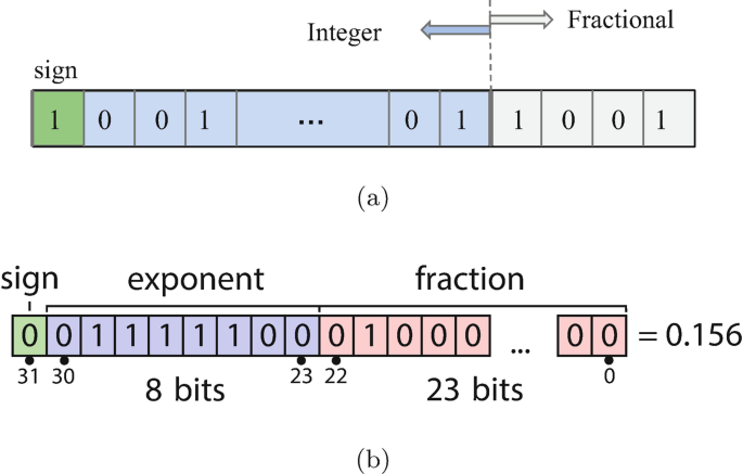
Fixed-point representation in (a) with a bit-width of 8 and a fractional length of 2 (left) and − 2 (right). On (b) the standard IEEE-754 representation of 32 bit floating-point values
-
Fixed-point representation: This representation uses two parameters: bit-width and fractional length. Negative fractional lengths can be used to represent powers of two. This representation is referred to as \(\mathcal {Q}\) (for quantized) in the rest of the chapter.

To evaluate the robustness of a given model to faults, we create a fault injection framework that takes a trained network as an input. While testing the model at inference time, bit-flips are injected in the network’s weights with a tunable injection rate. After each test, we report the overall accuracy under fault injection.
These tests are repeated 100 times for a statistically representative experiment. In each run, the engine generates a new set of errors and the injection of the generated errors is performed each run. We then report the accuracy distribution, i.e., the average accuracy, the maximum, the minimum, and the standard deviation for the test.
2.2 Results
The results were obtained on weights in single-precision floating point comparatively with quantized weights in terms of classification accuracy of the different networks. The results of different runs are presented as the mean and the standard deviation of the top-1 accuracy.
Figure 3 illustrates the result of comparing the floating-point and quantized representations. The results show that quantized models are surprisingly more robust to fault injection than the full precision models, which has been consistently observed for 4 different CNNs with different fault injection rates. We believe that the reason behind this observation is the error distance after injection denoted by \(\mathcal {A}\) in [10]. For instance, the \(\mathcal {Q}\) representation with 7 decimal bits and 1 integer bit will differ from the original value by at most ± 1. However, for the full precision representation, the error distance on activation can reach 3 × 1038 as observed in [10]. Therefore, since floating-point numbers are more sensitive to bit-flips than fixed-point representation, quantized networks tend to show higher robustness to errors, in addition to the area and power consumption gains.

Models accuracy under fault injection for weights representation with 8-bit fixed point (\(\mathcal {Q}\)) and 32-bit single-precision IEEE-754 (\(\mathcal {F}\))
3 ML Security
ML systems have been deployed in a variety of application domains, including security-sensitive and safety-critical applications [11]. However, ML models have been shown vulnerable to several security threats, including adversarial examples, which consist of additive noise carefully crafted to fool ML models.
3.1 Adversarial Attacks
Adversarial examples are additive perturbations to an input that are carefully crafted by an adversary to deceive the model and force it to output a wrong label. If adversaries succeed in manipulating the decisions of a ML classifier to their advantage, this can tamper with the security and integrity of the system, and potentially threaten the safety of people in some applications like autonomous vehicles. For example, adding adversarial noise to a stop sign that leads an autonomous car to wrongly classify it as a speed limit sign can lead to crashes and loss of life. In fact, adversarial examples have been shown effective under real-world settings [12,13,14]: that when printed out, an adversarially crafted image can fool the classifiers even under different lighting conditions and orientations. Therefore, understanding and mitigating these attacks is essential to developing safe and trustworthy intelligent systems.
Attacker Knowledge
When attacking a DNN-based model, we can distinguish two main attack scenarios based on attacker knowledge:
-
(i)
Black-box setting: the adversary has partial or no access to the victim model’s architecture and parameters. The adversary uses the results of querying the victim to reverse engineer the classifier and create a substitute model used to generate the adversarial examples. An illustration of this scenario is given by Fig. 4.
Fig. 4 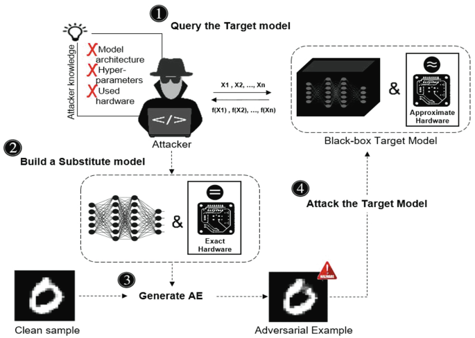
Illustration of a black-box attack setting
-
(ii)
White-box setting: in which the adversary has complete knowledge of the training data of the victim model in addition to the target model’s architecture and parameters. An illustration of this scenario is given by Fig. 5. (FGSM) [15] attack, Projected gradient descent (PGD) [16] attack, Carlini & Wagnar (C&W) [17] are the main white-box adversarial attacks.
Fig. 5 
Illustration of a white-box attack setting


The attacker intention is to slightly modify the source image so that it is classified incorrectly by the target model, without special preference towards any particular output which is known as untargeted attack. However, in a targeted attack, the attacker aims at a specified wrong target class.
Minimizing Injected Noise
An adversary, using information learned about the classifier, generates perturbations to cause incorrect classification under the constraint of minimizing this perturbation magnitude to avoid detection. For illustration purposes, consider a CNN used for image classification. More formally, given an original input image x and a target classification model f() s.t. f(x) = l, the problem of generating an adversarial example x∗ can be formulated as a constrained optimization [17]:
where \(\mathcal {D}\) is the distance metric used to quantify the similarity between two images and the goal of the optimization is to minimize this added noise, typically to avoid detection of the adversarial perturbations. l and l∗ are the two labels of x and x∗, respectively: x∗ is considered as an adversarial example if and only if the label of the two images are different (f(x) ≠ f(x∗)) and the added noise is bounded (\(\mathcal {D}(x,x^*) < \epsilon \) where \(\epsilon \geqslant 0 \)).
Distance Metrics
The adversarial perturbations should be visually imperceptible by a human eye. Since it is hard to model humans’ perception, three metrics have been practically used to measure the noise magnitude relatively to a given input, namely L0, L2, and L∞ [17]. Notice that these three metrics are special cases of the Lp norm defined as follows:
These metrics focus on different aspects of visual significance. For example, L0 evaluates the number of pixels with different values at corresponding positions in two inputs. L2 is the Euclidean distance between two images x and x∗, while L∞ is the maximum difference for all pixels at corresponding positions in the two images.
Adversarial Attacks Generation
Several methods have been proposed in the literature to generate adversarial examples. In the following we give a quick overview on the most popular ones:
Fast Gradient Sign Method (FGSM)
FGSM is a single-step, gradient-based, attack. An adversarial example is generated by calculating a one-step gradient update following the direction of the sign of the loss gradient over the input, which is the direction that maximizes the target model’s loss:
where ∇J() is the gradient of the loss function J and θ is the set of model parameters and 𝜖 is the perturbation magnitude budget.
Projected Gradient Descent (PGD)
PGD is a more efficient attack generation method; it is an iterative variant of FGSM where the adversarial noise is generated adaptively as follows:
where \(\mathcal {P}_{\mathcal {S}_x}()\) is a projection operator projecting the input into the feasible region \(\mathcal {S}_x\) and α is the added noise at each iteration. PGD find the perturbation that maximizes the loss of a model on a particular input while keeping the size of the perturbation lower than the budget due to the projection operator.
Carlini & Wagner (C&W)
This attack has 3 variants based on the used distance metric (l0, l2, l∞). It generates adversarial examples by solving the following optimization problem:

where \(\left \Vert \delta \right \Vert _2\) is the lowest noise that forces the model to misclassify. l(⋅) is the loss function defined as follows:
where Z(x) is the output of the layer before the softmax called logits. t is the target label, and κ is the attack confidence. An adversarial example is considered as successful if maxi ≠ t{Z(x)i}− Z(x)t ≤ 0.
3.1.1 Defenses Against Adversarial Attacks
To protect ML models against adversarial attacks, several defense techniques can be found in the literature. We briefly introduce the different categories and provide insights from Embedded Systems perspective.
Adversarial Training (AT)
AT is one of the most efficient state-of-the-art defense methods against adversarial attacks whose aim is to integrate the adversarial noise within the training process. It can be formulated as follows [16]:
where θ indicates the parameters of the classifier, \(\mathcal {L}_{c e}\) is the cross-entropy loss, \((x, y) \sim \mathcal {D}\) represents the training data sampled from a distribution \(\mathcal {D}\), and B(x, ε) is the allowed perturbation set. In this formulation, the inner maximization problem’s objective is to explore the “adversarial surrounding” of a given training point and to take into account, not only the sample but also the worst-case noise from an adversarial perspective. The outer minimization problem is the conventional training aiming at minimizing the loss function (which includes adversarial noise) [16].
Nonetheless, the drawback of AT is its significant computational intensivity compared to the baseline training process. This is obviously due to the nested optimization problems in the formulation that need to be solved iteratively.
Input Pre-processing (IP)
Input pre-processing is based on applying transformations to the input in order to remove adversarial perturbations [18, 19]. Transformations include the averaging, median, and Gaussian low-pass filters [19], as well as JPEG compression [20]. However, it has been shown that these defenses are vulnerable to white-box attacks [21]; in a white-box setting, where the adversary is aware of the defense, they can integrate the pre-processing function in the noise generation process. Furthermore, pre-processing requires computation overheads which is not suitable for resource-constrained devices such as Embedded Systems.
Gradient Masking (GM)
GM leverages regularization to make the model’s output less sensitive to input perturbations. Papernot et al. presented defensive distillation [22]. Nonetheless, this method is vulnerable to C&W attack [17]. Besides, GM techniques such as defensive distillation require a retraining process which results in time and energy overheads.
Randomization-Based Defenses
These techniques leverage randomness to protect systems from adversarial noise. Lecuyer et al. [23] propose that random noise be added to the first layer of the DNN and the output be estimated via a Monte Carlo simulation. Raghunathan et al. [24] evaluate only a tiny neural network. Estimating the model output requires a heavy Monte Carlo simulation with a number of different model inference runs online, which cannot be afforded under resource constraints.
These defense strategies either require changing the DNN structure, modifying the training process or retrain the model only against known adversarial threats, which results in considerable overheads in time, resource utilization and energy consumption. In the following, we present defense strategies that take into account this aspect, which we call Embedded Systems-friendly defenses.
3.2 Embedded Systems-Friendly Defenses
Another set of defense techniques are inspired by hardware-efficiency techniques such quantization [25, 26]. The authors in [27] proposed Defensive approximation (DA), which leverages approximate computing (AC) to build robust models.
3.2.1 Defensive Approximation
The demand on high-performance embedded and mobile devices has been drastically increasing in the past decades. However, the technology is physically reaching the end of Moore’s law, especially with the release of TSMC and Samsung 5 nm technology [28]. On the other hand, we observe that highly accurate computations might not be a must in all application domains. In fact, in a wide range of emerging applications, there is no specific accuracy requirements at the computing-element level, but rather a quality-of-service requirements on the system level. These application are inherently fault-tolerant by design and can relax the computational accuracy constraint. This observation has motivated the development of approximate computing (AC), a computing paradigm that trades power consumption with accuracy. The idea is to implement inexact/approximate elements that consume less energy, as far as the overall application tolerates the imprecision level in computation. This paradigm has been shown promising for inherently fault-tolerant applications such as deep learning, data analytics, and image/video/signal processing. Several AC techniques have been proposed in the literature and can be classified into three main categories based on the computing stack layer they target: software, architecture, and circuit level [29, 30].
Defensive approximation [27] tackles the problem of robustness to adversarial attacks from a new perspective, i.e., approximation in the underlying hardware, and leverages AC to secure DNNs. Specifically, at the lowest level, DA replaces exact conventional multipliers used in the convolution operations by an approximate multipliers. These approximate multiplier can generate inaccurate outputs, but the error distance needs to be under control. For this reason, the approximation occurs specifically in the mantissa multiplication, exclusively, to avoid high magnitude noise in the case of errors in the exponent or the sign bit of floating-point numbers. Subsequently, the convolution layers are built based on the approximate multipliers, which injects AC-induced noise within model layers. This noise is leveraged to protect DNNs against adversarial attacks. Moreover, in addition to the by-product gains in resources due to AC, this defense requires no retraining or fine-tuning of the protected model.
DA targets both robustness and energy/resource challenges. In fact, DA exploits the inherent fault tolerance of deep learning systems to provide resilience while also obtaining by-product gains of AC in terms of energy and resources. The AC-induced perturbations tend to help the classifier generalize and enhances its confidence and consequently enhance the classifier’s robustness. Figure 6 gives an overview on DA mechanism within a CNN. It shows the distribution of the error distance due to the approximate multiplier. This noise distribution propagates within the model and impacts the features map, thereby defusing the adversarial noise mechanism. In the following, we discuss the exploration of approximation space with regards to the baseline accuracy of the models.

Defensive approximation overview
3.2.1.1 Baseline Accuracy
Before exploring the impact of AC on the security of DNNs, the protected model needs to maintain models’ utility as a bottom line. For this reason, we explore the impact of the approximate multiplier on the accuracy for different levels of approximation, i.e., starting from approximating the full network, comparatively with having increasing exact layers along with the approximate model. Table 1 gives an overview on the utility as a function of the approximation level of the model for CIFAR-10 and ImageNet datasets.
3.2.1.2 Impact on Robustness
To evaluate the impact of AC on robustness, we consider a powerful adversary that has full access to the defense mechanism as well as the victim model architecture and parameters. Hence, we measure the model accuracy under adversarial examples created using different attacks for several noise budgets.
Figure 7 summarizes the effectiveness of DA defense against FGSM and PGD attacks for different noise budgets (ε). The approximate hardware prevents the attacker from generating efficient AE for deeper networks and complex data distribution. Even with a high amount of injected noise (𝜖 = 0.06), DA model accuracy remains as high as 90% under PGD attack.

Model accuracy for different noise budgets under white-box attack. (a) CIFAR-10 using FGSM. (b) CIFAR-10 using PGD. (c) ImageNet using FGSM. (d) ImageNet using PGD
3.2.2 Undervolting as a Defense
3.2.2.1 Approach
This approach explores using voltage over-scaling (VOS) as a lightweight defense against adversarial attacks [31]. It consists of reducing supply voltage at runtime, i.e., inference, without accordingly scaling down the frequency (Fig. 8). This creates stochastic hardware-induced noise at computation circuitry that is leveraged to defend DNNs against adversarial attacks. The rationale behind choosing VOS is as follows:
-
(i)
Stochastic noise: The impact of injecting random noise on DNNs robustness has been proven theoretically in [23, 32]. However, none of these works provides a practical implementation of the randomness source, especially one that does not require high overhead and considerable complexity to cope with Embedded ML requirements. This approach leverages a fundamental property of VOS, which is a stochastic behavior of the induced timing violations within the circuit.
-
(ii)
Controllable noise magnitude: While injected random noise can be used to improve the robustness of DNNs [23], its magnitude should be under control. In fact, injecting high magnitude noise can have drastic impact on baseline accuracy. Nonetheless, VOS-induced noise magnitude is directly controllable by the supply voltage.

Experimental setup for undervolted models robustness
3.2.2.2 Setup
To match the fault rates with the voltage levels, we used a Xilinx Zynq Ultrascale+ ZCU104 FPGA platform that hosts a VGG-16 CNN. The device’s Processing System (PS) includes a quad-core Arm Cortex-A53 applications processor (APU), as well as a dual-core Cortex-R5 real-time processor (RPU). We leveraged an external voltage controller, the Infineon USB005, to perform undervolting characterization on the FPGA device, which is connected to the board via an I2C wire. We can read and write the different voltage rail supplies to the board using PowerIRCenter GUI.
3.2.2.3 Impact on Robustness
Figure 9 shows the accuracy of the exact model and undervolted models for LeNet-5, AlexNet, and ResNet-18 CNNs under ℓ∞ and ℓ2 C&W attack. While the baseline exact model (hexact) yields high classification accuracy, it drops drastically under C&W attack reaching near 0 for ε = 0.4. Most importantly, approximate model with a fault rate fr = 10−4 maintains a high robustness (accuracy under attack) even for high magnitude ε. This observation holds for AlexNet and ResNet-18 as well.

Robustness of VOS-models under C&W attack for both ℓ∞ (top) and ℓ2 (bottom) metrics
While VOS offers a practical source of randomness that enhances DNNs robustness to adversarial attacks, it also comes with an obvious by-product gain in terms of power consumption, and offers an ad-hoc defense that does not require modifying the model or retraining it.
Trade-off
The results show that a VOS-induced noise protects DNNs against adversarial attacks. However, aggressive undervolting results in a drop in utility. A trade-off between accuracy and robustness with by-product power savings could be found, to achieve high-robustness models without accuracy drop. An example of a robustness/accuracy trade-off is depicted in Fig. 10. Notice that fr represent the fault rates, which are directly defined by the VOS level. The figure shows that with a simple space exploration, we can identify a sweet-spot for a given CNN that yields the highest possible robustness with the lowest possible accuracy drop.

An illustration of the accuracy/robustness trade-off for AlexNet with CIFAR-10 on HSJ. In the figure, fr = 0 indicates the exact model, hexact
3.3 Privacy
Confidentiality is a fundamental design property, especially for systems that process, store, or communicate private and sensitive data. In ML, insuring a model privacy consists in protecting the model against information leakage, whereby an adversary aims to infer sensitive information such as training data by interacting with the victim. In fact, the promising performance of ML systems spread their use to sensitive applications ranging from medical diagnosis in health-care to surveillance and biometrics. These models are trained on various data such as clinical/biomedical records, personal photos, genome data, financial, social, location traces, etc. Moreover, they are also trained with crowd-sourced data as cloud providers (e.g., Amazon AWS, Microsoft Azure, Google API) in a ML-as-a-Service fashion, which allow novice users to train models that often contains personally identifiable information.
ML models are vulnerable to privacy threats, which are critical when data confidentiality is an issue, e.g., when revealing the identity of the patients in clinical records. Membership Inference Attacks [33] aim at determining whether a data sample belongs to the training dataset. More generically, Property Inference Attacks [34] infer certain properties that hold only for a fraction of the training data, and are independent from the features that the DNN model aims to learn. On the other hand, Model Stealing methods [35] aim at duplicating the functionality of the ML model and extract its parameters, and Model Inversion Attacks [36] aim to infer sensitive features of the training data.
Towards avoiding these leakages of confidential information, several privacy-preserving techniques can be employed. Homomorphic Encryption (HE) ensures that the data remains confidential, since the attacker does not have access to the decryption keys. CryptoNets [37] apply HE to perform DNN inference on encrypted data, and the work of [38] extends the encryption to the complete training process. However, HE-based techniques are very costly in terms of execution time and resources.
Another state-of-the-art technique towards privacy-preserving ML is Differential Privacy (DP) which consists of injecting random noise to the stochastic gradient descent process (Noisy SGD) [39], or through Private Aggregation of Teacher Ensembles (PATE) [40], in which the knowledge learned by an ensemble of “teacher” models is transferred to a “student” model. While DP is one of the most efficient defenses against information leakage, it comes at a considerable cost in terms of utility, i.e., it results in a baseline accuracy drop.
Training a deep neural network requires a large amount of data, which represents practically the most valuable asset in ML ecosystems. In some specific applications, data protected by privacy regulations and user level agreements. These can be specific to application domains such as HIPPA regulations in the US which prohibits patients’ data sharing and GDPR in Europe, which is more generic in regulating user data collection [41]. Therefore, in medical applications, a given health institution might not be able to collect enough data that is representative and relevant to train an efficient ML model.
In another scenarios, data may be created on Edge devices, but owners are reluctant to sharing it due to privacy concerns (industrial applications, text messages, etc.), bandwidth challenges, or both.
Federated learning (FL) recently emerged as a potential solution to overcome these aforementioned issues. Specifically, FL allows train ML models collaboratively between different nodes without sharing their local data [42]. FL allows multiple participants (also called clients) to train local models and then consolidate those models into a global model. This global model benefits from all client data, without directly sharing the data, preserving data privacy. Each client trains its model on its private data, and then communicates model updates to a central server (also called aggregator). By avoiding communicating the data to a central back end for training, this data remains local to each client and therefore private. Moreover, distributing the training leads to benefits in performance and network bandwidth. In an FL model, each participant updates the global model by training it on its local data and shares the metadata with a central server. Only the trained local model updates are shared, and the local data to each client remains private. The server aggregates the local model updates into a single federated model and shares this model with the participants, allowing them to benefit from a model trained on the overall data. The federated model can continue to be refined as more data becomes available. This process is illustrated in Fig. 11.

An overview on FL setting: Client devices send locally trained model updates to server for aggregation of the federated model
While FL has been branded by major companies such as Google as a privacy-preserving solution, it has been shown that it is vulnerable to several attacks that can jeopardize its and confidentiality:
Model Poisoning and Data Poisoning
Each of the clients in FL setting is able to arbitrarily change its local model maliciously that they send to server. The model can be manipulated either directly through its parameters or indirectly by poisoning the local training set to degrade the quality of the aggregated model making it misclassify more often, or be more susceptible to adversarial inputs. In model poisoning, a malicious client attempts to change the global model by poisoning their local model parameters directly [43]. In contrast, in data poisoning, the attacker manipulates its local training samples, affecting the model’s performance indirectly throughout a substantial portion of the input space [44].
Deep Leakage from Gradients
With access to the gradient of a particular client, an adversary is able reconstruct the training samples of the client. In fact, attacks like Deep Leakage from gradient (DLG) [45] and iDLG [46] show the possibility to reconstruct training data samples from raw gradients only. The recovered images are pixel wise accurate, and generated through an optimization problem aiming at reducing the difference between the gradient of a given candidate input and the real gradient.
Defenses and Limits
Differential Privacy has been used as a defense against data leakage [39]. However, it does not protect against poisoning attacks. Moreover, secure aggregation techniques such as [47] aim at preventing the server from accessing the individual model updates, while allowing the aggregation operation. However, this defense results by construction in an impossibility to detect integrity attacks.
To defend against integrity attacks, and limit the influence of individual participants, robust aggregation techniques have been proposed (also called Byzantine-tolerant aggregation) [48, 49].
Fairness
FL approach is designed under the assumption of non-iid data. The incentive of participants to share their model updates generated on local data is to enhance the model accuracy, specifically on their own data distribution. However, robust aggregation techniques consider the tail of the gradient updates distribution as a potential integrity attack and cuts it off in the aggregation phase. Therefore, users with “atypical” data, i.e., in the tail of the overall users data distribution will not benefit from the FL setting since their contributions are discarded by the robust aggregation mechanism [50]. This results in a fairness problem: users with minority and atypical data distributions will be disadvantaged by the FL setting.
Open Problems
FL offers an interesting solution towards privately sharing “knowledge representations” without necessarily sharing raw data, which allows to train more generalizing and efficient models. However, a three objectives that are necessary for FL deployment seem to be difficult to obtain simultaneously, i.e., privacy, integrity, and fairness. In fact, secure aggregation techniques solve the privacy problem and open an attack surface on the model integrity. On the other hand, tackling the integrity problem with robust aggregation schemes results in the loss of the global model fairness.
We believe that a fundamental problem to solve by the community is finding interesting and adaptive trade-off between these three objectives.
4 Conclusion
This chapter focuses on three aspects of ML trustworthiness, especially in the context of embedded systems and the Edge:
-
(i)
The first is ML models robustness to errors, either due to hardware reliability issues or deliberately injected by malicious actors.
-
(ii)
The second aspect is the security of ML models, especially from an adversarial ML perspective. More specifically, we explored defense techniques that are Embedded Systems-friendly, i.e., that do not result in a high overhead in power consumption or hardware resources.
-
(iii)
The third is the privacy problem, where we focused on federated learning as an emerging training paradigm that is compatible with Embedded Systems and IoT applications.
References
Ben Khalifa, A., Alouani, I., Mahjoub, M.A., Rivenq, A.: A novel multi-view pedestrian detection database for collaborative intelligent transportation systems. Fut. Gener. Comput. Syst. 113, 506–527 (2020). https://doi.org/10.1016/j.future.2020.07.025
Jegham, I., Khalifa, A.B., Alouani, I., Mahjoub, M.A.: Soft spatial attention-based multimodal driver action recognition using deep learning. IEEE Sensors J. 21(2), 1918–1925 (2021). https://doi.org/10.1109/JSEN.2020.3019258
Al-Qizwini, M., Barjasteh, I., Al-Qassab, H., Radha, H.: Deep learning algorithm for autonomous driving using GoogLenet. In: 2017 IEEE Intelligent Vehicles Symposium (IV), pp. 89–96. IEEE, Piscataway (2017)
Deng, L., Liu, Y.: Springer, Berlin (2018)
Pierson, H.A., Gashler, M.S.: Deep learning in robotics: a review of recent research. Advanced Robotics 31(16), 821–835 (2017)
Miotto, R., Wang, F., Wang, S., Jiang, X., Dudley, J.T.: Deep learning for healthcare: review, opportunities and challenges. Briefings in bioinformatics 19(6), 1236–1246 (2018)
Masanet, E., Shehabi, A., Lei, N., Smith, S., Koomey, J.: Recalibrating global data center energy-use estimates. Science 367(6481), 984–986 (2020). https://doi.org/10.1126/science.aba3758
Kim, Y., Daly, R., Kim, J.S., Fallin, C., Lee, J., Lee, D., Wilkerson, C., Lai, K., Mutlu, O.: Flipping bits in memory without accessing them: An experimental study of DRAM disturbance errors. In: ACM/IEEE 41st International Symposium on Computer Architecture, ISCA 2014, Minneapolis, pp. 361–372 (2014). https://doi.org/10.1109/ISCA.2014.6853210
Liu, Q., Liu, T., Liu, Z., Wang, Y., Jin, Y., Wen, W.: Security analysis and enhancement of model compressed deep learning systems under adversarial attacks. In: Proceedings of the 23rd Asia and South Pacific Design Automation Conference. ASPDAC ’18, pp. 721–726. IEEE Press, Piscataway (2018). http://dl.acm.org/citation.cfm?id=3201607.3201772
Neggaz, M.A., Alouani, I., Lorenzo, P.R., Niar, S.: A reliability study on CNNs for critical embedded systems. In: 2018 IEEE 36th International Conference on Computer Design (ICCD), pp. 476–479. IEEE (2018)
Neggaz, M.A., Alouani, I., Niar, S., Kurdahi, F.J.: Are CNNs reliable enough for critical applications? An exploratory study. IEEE Des. Test 37(2), 76–83 (2020). https://doi.org/10.1109/MDAT.2019.2952336
Eykholt, K., Evtimov, I., Fernandes, E., Li, B., Rahmati, A., Xiao, C., Prakash, A., Kohno, T., Song, D.: Robust physical-world attacks on deep learning visual classification. In: 2018 IEEE Conference on Computer Vision and Pattern Recognition, CVPR 2018, Salt Lake City, UT, USA, June 18–22, 2018, pp. 1625–1634. Computer Vision Foundation/IEEE Computer Society (2018). https://doi.org/10.1109/CVPR.2018.00175
Man, Y., Li, M., Gerdes, R.M.: GhostImage: Remote perception attacks against camera-based image classification systems. In: 23rd International Symposium on Research in Attacks, Intrusions and Defenses, RAID 2020, San Sebastian, Spain, October 14–15, 2020, 317–332 (2020)
Tarchoun, B., Alouani, I., Ben Khalifa, A., Mahjoub, M.A.: Adversarial attacks in a multi-view setting: An empirical study of the adversarial patches inter-view transferability. In: 2021 International Conference on Cyberworlds (CW), pp. 299–302 (2021). https://doi.org/10.1109/CW52790.2021.00057
Goodfellow, I.J., Shlens, J., Szegedy, C.: Explaining and harnessing adversarial examples. In: Bengio, Y., LeCun, Y. (eds.): In: 3rd International Conference on Learning Representations, ICLR 2015, San Diego, CA, USA, May 7–9, 2015, Conference Track Proceedings (2015)
Madry, A., Makelov, A., Schmidt, L., Tsipras, D., Vladu, A.: Towards deep learning models resistant to adversarial attacks. In: 6th International Conference on Learning Representations, ICLR 2018, Vancouver, BC, Canada, April 30–May 3, 2018, Conference Track Proceedings (2018)
Carlini, N., Wagner, D.A.: Towards evaluating the robustness of neural networks. In: 2017 IEEE Symposium on Security and Privacy, SP 2017, San Jose, CA, USA, May 22–26, 2017, pp. 39–57 (2017). https://doi.org/10.1109/SP.2017.49
Guesmi, A., Alouani, I., Baklouti, M., Frikha, T., Abid, M.: Sit: stochastic input transformation to defend against adversarial attacks on deep neural networks. IEEE Design Test 1–1 (2021). https://doi.org/10.1109/MDAT.2021.3077542
Osadchy, M., Hernandez-Castro, J., Gibson, S., Dunkelman, O., Pérez-Cabo, D.: No bot expects the DeepCAPTCHA! Introducing immutable adversarial examples, with applications to CAPTCHA generation. IEEE Trans. Inform. Forensics Secur. 12(11), 2640–2653 (2017)
Das, N., Shanbhogue, M., Chen, S.-T., Hohman, F., Chen, L., Kounavis, M.E., Chau, D.H.: Keeping the Bad Guys Out: Protecting and Vaccinating Deep Learning with JPEG Compression (2017)
Chen, J., Wu, X., Rastogi, V., Liang, Y., Jha, S.: Towards understanding limitations of pixel discretization against adversarial attacks. In: 2019 IEEE European Symposium on Security and Privacy (EuroS&P), pp. 480–495. IEEE (2019)
Papernot, N., McDaniel, P., Wu, X., Jha, S., Swami, A.: Distillation as a defense to adversarial perturbations against deep neural networks. In: 2016 IEEE Symposium on Security and Privacy (SP), pp. 582–597 (2016). https://doi.org/10.1109/SP.2016.41
Lecuyer, M., Atlidakis, V., Geambasu, R., Hsu, D., Jana, S.: Certified robustness to adversarial examples with differential privacy. In: 2019 IEEE Symposium on Security and Privacy (SP), pp. 656–672 (2019)
Raghunathan, A., Steinhardt, J., Liang, P.: Certified Defenses against Adversarial Examples (2018)
Lin, J., Gan, C., Han, S.: Defensive quantization: when efficiency meets robustness. In: 7th International Conference on Learning Representations, ICLR 2019, New Orleans, LA, USA, May 6–9, 2019 (2019)
Khalid, F., Ali, H., Tariq, H., Hanif, M.A., Rehman, S., Ahmed, R., Shafique, M.: QuSecNets: quantization-based defense mechanism for securing deep neural network against adversarial attacks. In: 25th IEEE International Symposium on On-Line Testing and Robust System Design, IOLTS 2019, Rhodes, Greece, July 1–3, 2019, 182–187 (2019). https://doi.org/10.1109/IOLTS.2019.8854377
Guesmi, A., Alouani, I., Khasawneh, K.N., Baklouti, M., Frikha, T., Abid, M., Abu-Ghazaleh, N.B.: Defensive approximation: securing CNNs using approximate computing. In: ASPLOS ’21: 26th ACM International Conference on Architectural Support for Programming Languages and Operating Systems, Virtual Event, USA, April 19–23, 2021, pp. 990–1003 (2021). https://doi.org/10.1145/3445814.3446747
Moore, S.K.: Another step toward the end of Moore’s law: Samsung and TSMC move to 5-nanometer manufacturing—[news]. IEEE Spectr. 56(6), 9–10 (2019). https://doi.org/10.1109/MSPEC.2019.8727133
Guesmi, A., Alouani, I., Baklouti, M., Frikha, T., Abid, M., Rivenq, A.: Heap: a heterogeneous approximate floating-point multiplier for error tolerant applications. In: Proceedings of the 30th International Workshop on Rapid System Prototyping (RSP’19). RSP ’19, pp. 36–42. Association for Computing Machinery, New York (2019). https://doi.org/10.1145/3339985.3358495
Alouani, I., Ahangari, H., Ozturk, O., Niar, S.: A novel heterogeneous approximate multiplier for low power and high performance. IEEE Embedded Syst. Lett. 10(2), 45–48 (2018). https://doi.org/10.1109/LES.2017.2778341
Islam, S., Alouani, I., Khasawneh, K.N.: Lower voltage for higher security: using voltage overscaling to secure deep neural networks. In: 2021 IEEE/ACM International Conference On Computer Aided Design (ICCAD), pp. 1–9 (2021). https://doi.org/10.1109/ICCAD51958.2021.9643551
Cohen, J.M., Rosenfeld, E., Kolter, J.Z.: Certified adversarial robustness via randomized smoothing. In: Proceedings of the 36th International Conference on Machine Learning, ICML 2019, 9-15 June 2019, Long Beach, California, USA, vol. 97, pp. 1310–1320 (2019)
Shokri, R., Stronati, M., Song, C., Shmatikov, V.: Membership inference attacks against machine learning models. In: 2017 IEEE Symposium on Security and Privacy, SP 2017, San Jose, CA, USA, May 22–26, 2017, pp. 3–18 (2017). https://doi.org/10.1109/SP.2017.41
Ganju, K., Wang, Q., Yang, W., Gunter, C.A., Borisov, N.: Property inference attacks on fully connected neural networks using permutation invariant representations. In: Proceedings of the 2018 ACM SIGSAC Conference on Computer and Communications Security, CCS 2018, Toronto, ON, Canada, October 15–19, 2018, pp. 619–633 (2018). https://doi.org/10.1145/3243734.3243834
Tramèr, F., Zhang, F., Juels, A., Reiter, M.K., Ristenpart, T.: Stealing machine learning models via prediction APIs. In: 25th USENIX Security Symposium, USENIX Security 16, Austin, TX, USA, August 10–12, 2016, pp. 601–618 (2016)
Fredrikson, M., Jha, S., Ristenpart, T.: Model inversion attacks that exploit confidence information and basic countermeasures. In: Proceedings of the 22nd ACM SIGSAC Conference on Computer and Communications Security, Denver, CO, USA, October 12–16, 2015, pp. 1322–1333 (2015). https://doi.org/10.1145/2810103.2813677
Gilad-Bachrach, R., Dowlin, N., Laine, K., Lauter, K.E., Naehrig, M., Wernsing, J.: Cryptonets: Applying neural networks to encrypted data with high throughput and accuracy. In: Proceedings of the 33nd International Conference on Machine Learning, ICML 2016, New York City, NY, USA, June 19–24, 2016, vol. 48, pp. 201–210 (2016)
Nandakumar, K., Ratha, N.K., Pankanti, S., Halevi, S.: Towards deep neural network training on encrypted data. In: IEEE Conference on Computer Vision and Pattern Recognition Workshops, CVPR Workshops 2019, Long Beach, CA, USA, June 16–20, 2019, pp. 40–48 (2019). https://doi.org/10.1109/CVPRW.2019.00011
Abadi, M., Chu, A., Goodfellow, I.J., McMahan, H.B., Mironov, I., Talwar, K., Zhang, L.: Deep learning with differential privacy. In: Proceedings of the 2016 ACM SIGSAC Conference on Computer and Communications Security, Vienna, Austria, October 24–28, 2016, pp. 308–318 (2016). https://doi.org/10.1145/2976749.2978318
Papernot, N., Song, S., Mironov, I., Raghunathan, A., Talwar, K., Erlingsson, Ú.: Scalable private learning with PATE. In: 6th International Conference on Learning Representations, ICLR 2018, Vancouver, BC, Canada, April 30–May 3, 2018, Conference Track Proceedings (2018)
Annas, G.J., et al.: HIPAA regulations-a new era of medical-record privacy? N. Engl. J. Med. 348(15), 1486–1490 (2003)
Kairouz, P., McMahan, H.B., Avent, B., Bellet, A., Bennis, M., Bhagoji, A.N., Bonawitz, K., Charles, Z., Cormode, G., Cummings, R., et al.: Advances and open problems in federated learning (2019). arXiv preprint arXiv:1912.04977
Bagdasaryan, E., Veit, A., Hua, Y., Estrin, D., Shmatikov, V.: How to backdoor federated learning. In: International Conference on Artificial Intelligence and Statistics, pp. 2938–2948. PMLR (2020)
Jere, M.S., Farnan, T., Koushanfar, F.: A taxonomy of attacks on federated learning. IEEE Secur. Privacy 19(2), 20–28 (2020)
Zhu, L., Han, S.: Deep Leakage from Gradients, pp. 17–31. Federated Learning (2020)
Zhao, B., Mopuri, K.R., Bilen, H.: iDLG: Improved deep leakage from gradients (2020). arXiv preprint arXiv:2001.02610
Chen, Y., Su, L., Xu, J.: Distributed statistical machine learning in adversarial settings: Byzantine gradient descent. Proc. ACM Meas. Anal. Comput. Syst. 1(2), 1–25 (2017)
Damaskinos, G., El-Mhamdi, E.-M., Guerraoui, R., Guirguis, A., Rouault, S.: AggregaThor: byzantine machine learning via robust gradient aggregation. Proc. Mach. Learn. Syst. 1, 81–106 (2019)
Rajput, S., Wang, H., Charles, Z., Papailiopoulos, D.: Detox: a redundancy-based framework for faster and more robust gradient aggregation. In: Advances in Neural Information Processing Systems, vol. 32 (2019)
Yu, T., Bagdasaryan, E., Shmatikov, V.: Salvaging federated learning by local adaptation (2020). arXiv preprint arXiv:2002.04758
Author information
Authors and Affiliations
Corresponding author
Editor information
Editors and Affiliations
Rights and permissions
Copyright information
© 2024 The Author(s), under exclusive license to Springer Nature Switzerland AG
About this chapter

Cite this chapter
Alouani, I. (2024). On the Challenge of Hardware Errors, Adversarial Attacks and Privacy Leakage for Embedded Machine Learning. In: Pasricha, S., Shafique, M. (eds) Embedded Machine Learning for Cyber-Physical, IoT, and Edge Computing. Springer, Cham. https://doi.org/10.1007/978-3-031-40677-5_19
Download citation
DOI: https://doi.org/10.1007/978-3-031-40677-5_19
Published:
Publisher Name: Springer, Cham
Print ISBN: 978-3-031-40676-8
Online ISBN: 978-3-031-40677-5
eBook Packages: EngineeringEngineering (R0)