
Abstract
Recent studies have shown that Machine Learning (ML) algorithm suffers from several vulnerability threats. Among them, adversarial attacks represent one of the most critical issues. This chapter provides an overview of the ML vulnerability challenges, with a focus on the security threats for Deep Neural Networks, Capsule Networks, and Spiking Neural Networks. Moreover, it discusses the current trends and outlooks on the methodologies for enhancing the ML models’ robustness.
Access provided by Autonomous University of Puebla. Download chapter PDF
Keywords
- Machine learning security
- Adversarial attacks
- Robustness
- Deep Neural Networks
- Capsule Networks
- Spiking Neural Networks
1 Introduction
The use-cases of Machine Learning (ML) applications have been significantly growing in recent years. Among the ML models, Deep Neural Networks (DNNs), which stack several layers of neurons, have demonstrated to solve complex tasks with high accuracy. Capsule Networks (CapsNets) have established as prominent ML models due to their high learning capabilities. Moreover, Spiking Neural Networks (SNNs) emerged as biologically plausible models, in which their spike event-based communication provides energy-efficient capabilities to be employed in low-power and resource-constrained devices [9, 10].
On the other hand, ML systems are expected to be reliable against multiple security threats. Several studies highlighted that one of the most critical issues is represented by the adversarial attacks, i.e., small and imperceptible input perturbations that cause misclassifications. Moreover, as highlighted in Fig. 1, also other ML vulnerabilities cause serious concerns questioning the deployment of ML models in safety-critical applications. Therefore, the ML community analyzed and proposed several attack methodologies and defensive countermeasures [77]. While the attacks and defenses for DNNs have been extensively studied, the security of advanced ML models such as CapsNets and SNNs is still in its emerging phase and needs more thorough investigations.

Vulnerability threats for ML-based systems, their manifestation and impact on their functionality
After discussing the security challenges for ML systems and the taxonomy of adversarial ML, this chapter provides an overview of the security threats for DNNs, CapsNets, and SNNs, focusing on recent advancements, current trends, and unique possibilities for specific ML models to enhance their robustness.
2 Security Challenges for ML
Recent works [14, 77, 78, 96] have shown that ML-based systems are vulnerable to different types of security and reliability threats (see Fig. 1), which can span from maliciously injected perturbations, such as adversarial attacks, hardware Trojans, or injected faults, to natural misfunctioning of the system, like permanent faults generated during chip fabrication, aging, and process variations. Moreover, the leakage of sensitive and confidential data, including the intellectual property of the ML model (e.g., architecture and parameters) and training dataset, have raised several privacy issues. While the adversarial ML issues will be extensively discussed in the rest of the chapter, this section briefly introduces the other types of vulnerabilities.
2.1 ML Privacy
Due to the massive performance and computational power of high-end GPU-HPC workstations, it is possible to conduct ML tasks using a massive amount of data on a large scale. If such data is collected from users’ private information, such as private images, interests, web searches, and clinical records, the ML deployment toolchain will have access to sensitive information that could potentially be mishandled. The privacy attacks for ML can be classified into two categories, namely Model Extraction Attacks and Model Inversion Attacks. While the former category aim at extracting private information of the ML model (e.g., model parameter, model architecture), the latter threatens the sensitive features of the training data.
-
Model Extraction Attacks: The goal of the adversary is to duplicate the parameters and hyperparameters of the model to provide ML services, and to compromise the ML algorithms’ confidentiality and intellectual property of the service provider [87, 92].
-
Model Inversion Attacks: The adversary aims to infer sensitive information from the training data. Membership inference attacks [81] can infer whether a sensitive record belongs to the training set when the ML model is overfitted, While Property Inference Attacks [19] infer specific properties that only hold for a fraction of the training data.
There are currently four possible categories of techniques that can be applied to avoid these leakages of sensitive information:
-
Differential Privacy: The goal is to prevent the adversary from inferring whether a specific data was used to train the target model, such that the ML algorithm learns to extract features of the training data without disclosing sensitive information about individuals. The privacy is guaranteed through a randomization mechanism, which could be based on injecting noise into the stochastic gradient descent process (Noisy SGD [1]) or through the Private Aggregation of Teacher Ensembles (PATE) method [65], in which a “student” model receives the knowledge transferred from an ensemble of “teacher” models.
-
Homomorphic Encryption: It is an encryption scheme \(x \rightarrow y\), in which the ML computations are conducted on ciphertexts y, and the decrypted output in plaintext x matches the result that would have been computed without encryption. As long as the decryption key is unknown to the adversary, the data remains confidential. Since the Fully Homomorphic Encryption (FHE) system [20] dramatically increases the computational complexity of the ML algorithm, a partial homomorphic encryption system [63] which supports only certain operations in the ciphertext domain, such as additions or multiplications, is more suited for complex computations. In the context of ML, CryptoNets [21] performs DNN inference on encrypted data, while Nandakumar et al. [60] extends the encryption support to the whole training process.
-
Secure Multi-Party Computation: The basic idea consists of distributing the training/testing data across multiple servers and training/inferring the ML model together, while each server does not have access to the training/testing data of the other servers. Different privacy-preserving ML protocols have been proposed, including SecureML [59], MiniONN [44], DeepSecure [74], Gazelle [31], and SecureNN [91].
-
Trusted Execution Environment: Additional hardware is used to create a secure and isolated computation environment in which the ML algorithms are executed [47]. In this way, the e integrity and confidentiality of the data and codes loaded inside the protected regions are guaranteed.
However, these privacy-preserving methods significantly increase the computational overhead and require customization for specific ML models at the software and hardware levels to improve the efficiency of computations.
2.2 Fault Injection and Hardware Trojans on ML Systems
Hardware-level security vulnerabilities for ML systems include fault injection techniques (e.g., bit-flips) and the injected hardware Trojans into ML accelerators. Generically speaking, an adversary can flip the bits of data stored into the SRAM and DRAM memory cells through laser injection [2] or Row-Hammer attacks [35].
-
Fault Injection Attack Methodologies aim at finding the most sensitive locations in which to inject faults [45, 89]. The Bit-Flip Attack [72] finds the most vulnerable bits of the ML model parameters using a progressive bit search method, while the Practical Fault Attack [7] injects faults into ML activations.
-
Hardware Trojans are maliciously introduced hardware injected during chip fabrication that only activate when triggered. They represent serious threats when the hardware devices are manufactured in off-shore fabrication facilities, thus increasing the risk of facing untrusted supply chains. In the context of ML accelerators, Clements et al. [12] designed hardware Trojans for the ML activation function, and in NeuroAttack, the Trojan consists of flipping the values of certain bits of ML models. In both methods, the hardware Trojan is triggered by a carefully designed input pattern.
The defensive countermeasures to mitigate against the above-discussed vulnerabilities are based on improving the resiliency of ML accelerators and memory systems and detecting Trojans.
-
Fault tolerance methods, similarly to the soft error mitigation methodologies, aim at improving the resiliency of ML applications. Such defensive techniques are based on hardware redundancy [62], range restriction [11], or weight reconstruction [40]. More specifically, the algorithm-based fault tolerance (ABFT) method [97] detects and corrects errors in the convolutional layers.
-
Trojan detection methods are based on runtime monitoring [18] of the ML accelerator. The operations executed in the hardware device are constantly monitored, and any eventual functionality violation due to an inserted hardware Trojan or other reasons can be immediately detected and notified.
2.3 ML Systems Reliability Threats
Unlike the vulnerability threats that are intentionally injected by malicious adversaries, ML systems are subjected to reliability threats that undermine their correct functionality. The continuous underscaling of the technology nodes in which the chips are fabricated has significantly increased the probability that hardware circuits are affected by permanent or transient faults and has accelerated the aging process.
-
Permanent Faults: These process variations represent imperfections that are generated during the fabrication of integrated circuits [71]. High rates of such process variations result in permanent faults, which dramatically decrease the yield of the wafer fabrication.
-
Transient Faults: Soft errors are bit-flips caused by high-energy particle strikes or induced by other radiation events [6]. They are categorized as transient errors since the faulty cells are not permanently damaged, but these faults vanish once new data is written into the same locations.
-
Aging: The electronic circuits gradually degrade over time [32], due to various physical phenomena, like Hot Carrier Injection (HCI), Bias Temperature Instability (BTI), and Electromigration (EM). These effects can manifest as transistors’ threshold voltage increase, which causes timing errors and permanent faults over time.
Conventional fault mitigation techniques such as Dual Modular Redundancy (DMR) [88], Triple Modular Redundancy (TMR) [48], and Error-Correcting Codes (ECC) [69] can be applied, but they incur huge overheads, which makes them impractical for ML applications. Therefore, ad-hoc cost-effective mitigation techniques need to be applied.
-
Permanent faults mitigation: To mitigate permanent faults due to process variations in ML accelerators, different techniques have been proposed. Fault-Aware Training (FAT) and Fault-Aware Pruning (FAP) [95] incorporate the information of faults into the training process and bypass the faulty components. To avoid the re-training overhead, Fault-Aware Mapping techniques such as SalvageDNN [28] are based on mapping the least significant weights on the faulty units.
-
Soft error mitigation: To mitigate transient faults, generic fault-tolerant methods like Ranger [11] and ABFT [97] can be applied. Moreover, FT-ClipAct [30] uses clipped activation functions that are mapped into pre-specified values within a range that has the lowest impact on the output, and Sanity-Check [61] protects fully connected and convolutional layers of ML models employing spatial and temporal checksums that exploit the linearity property.
-
Aging mitigation: The effects of timing errors that occur in the computational units of ML accelerators can be mitigated with ThUnderVolt [94] and GreenTPU [64]. The NBTI aging of on-chip SRAM-based memory cells in ML accelerators is mitigated with the DNN-Life framework [29] that employs read and write transducers to balance the duty-cycle in each SRAM cell.
3 Taxonomy of Adversarial ML
Given an ML model M, an input x, and its output prediction label ytrue, the goal of classical ML is to make a correct prediction, i.e., the predicted output y = M(x) is equal to ytrue. On the contrary, an adversarial attack method aims at generating a misclassification by introducing a small noise ε to the input, such that the adversarial example x′ = x + ε is incorrectly classified (M(x′) ≠ ytrue). Due to the wide variety of adversarial attack typologies and threat models, it is important to define a common taxonomy for their categorization. Towards this, we discuss four different features of adversarial attacks and their possible types. An overview of the taxonomy is shown in Fig. 2.

Categorization of different types of adversarial attack methods and their taxonomy
-
Attacker Knowledge: It refers to what is the threat model in which the adversary operates and what are the accessible data and features. In white-box attacks, the adversary has full knowledge about the ML model, its parameters, the training algorithm, and the training data. On the contrary, black-box attacks assume no knowledge about the ML model. Hence the adversary can only craft an adversarial example by sending a series of queries and analyzing the vulnerability based on the corresponding outputs. Moreover, in the literature, there exist different attacker knowledge assumption models referred to as grey-box attacks, in which the adversary knows more features than for black-box attacks, but does not have full access like under the white-box assumption.
-
Adversarial Goal: It refers to the scope of the attack algorithm. If the goal is simply a misclassification, the attack is untargeted since any class different from the correct one can be the prediction of the adversarial example. On the other hand, in a targeted attack, the adversary produces adversarial examples that force the output of the ML model to predict a specific class.
-
Phase of ML Flow: It refers to the stage of the ML development in which the adversary operates. In training attacks, the adversary poisons the training data by injecting carefully designed samples to force the ML model to learn wrong features that can later be used to generate specific misclassifications. On the contrary, in evasion attacks that operate at the inference stage, the adversary tries to evade the system by crafting malicious samples that force the ML model to make false predictions.
-
Evaluation Metrics: It refers to the quantitative methods for measuring the strengths of the attacks, and easily accessible comparison metrics. To evaluate the robustness of the attack, the success rate measures the number of adversarial examples that are misclassified by the ML model. Since a well-designed attack needs to be imperceptible, i.e., hardly distinguishable from the original input by a human eye, the perturbation measures the distance between the adversarial example and the original (clean) input.
4 Security for DNNs
Due to their high accuracy on many tasks, DNNs are prime candidate algorithms to be applied to safety-critical applications. However, due to the security vulnerabilities that undermine their correct functionality, several defensive countermeasures need to be applied. An overview of adversarial attacks and defenses applied to the DNN design flow is shown in Fig. 3.

Adversarial attacks and defenses applied in different stages of the DNN design flow
4.1 Adversarial Attacks
As previously discussed, the adversarial attacks can be categorized into different types based on the adversary’s knowledge, goal, and phase of the ML flow. Due to the mainstream usage of DNNs, several attack methodologies have been proposed. The following list discusses the most prominent ones:
-
Poisoning Attacks: At the training stage, the training data can be poisoned with contaminated inputs. Based on the principles of Genetic Adversarial Networks (GANs), Goodfellow et al. [22] devised a procedure to generate samples similar to the training set, having almost identical distribution. This method inspired many of the successive adversarial attack methodologies. Poisoning Attacks [76] alter the training dataset to modify the decision boundaries of the DNN classifiers. Backdoor Attacks [24] aim at training the DNN for a carefully crafted noise pattern (acting as a backdoor) while maintaining high accuracy on its intended task. However, when such a backdoor trigger is present at the input of the DNN, a targeted misclassification is achieved.
-
Evasion Attacks: Different evasion attack methodologies were proposed. In white-box settings, gradient-based attacks like the Fast Gradient Sign Method (FGSM) [23] and its iterative version, the Projected Gradient Descent (PGD) [50] exploit the gradient of the DNN output predictions w.r.t. the inputs to craft the adversarial perturbations as imperceptible noise that make the DNN classifier cross the decision boundary. In black-box settings, the One Pixel Attack [85] demonstrated to misclassify DNN models by changing only one pixel intensity. fakeWeather attacks [55] emulate the effect of atmospheric conditions to fool DNNs. Decision-based attacks [8] are a subset of evasion attacks in which the adversary does not have access to the output probabilities but only to the prediction. For instance, the FaDec attack [34] jointly optimizes the number of queries and the perturbation distance between the adversarial example and the clean example to fool DNNs.
-
Attacks in the Physical World: While the aforementioned attacks mainly make modifications in the experimental settings, the adversarial attacks can also be applied in real life by introducing physical modifications [38]. Examples of physical world attacks have been showcased in the context of road sign classification by adding stickers [17], in the context of object detection by adding adversarial patches [86], or in face detection using eyeglasses with special frames [79].
4.2 Adversarial Defenses
The large variety of adversarial attacks led to the design of several types of defenses, which can be summarized and grouped into the following categories:
-
Poisoning Defenses: To mitigate against poisoning attacks, several defensive countermeasures have been proposed. Outlier detection-based defenses [67] filter out training sample outliers, which most likely correspond to poisoned samples. Since typically backdoor attacks exploit the sparsity of DNNs, the Fine-Pruning method [46] defends against backdoor attacks by eliminating the neurons that are dormant for clean inputs in the backdoor network.
-
Data Augmentation: The basic principle of Adversarial Training [50] is to extend the training example with the adversarial examples, for instance, generated with the PGD attack. In this way, the DNN models achieve higher robustness against such perturbations. This method is considered very effective to defend against adversarial attacks, but its high computation overhead pushes the community to search for efficient optimizations of this procedure.
-
Quantization: The optimization techniques employed to improve the energy -efficiency of DNNs can also achieve higher robustness against adversarial attacks. The Defensive Quantization method [42] demonstrated that the adversarial noise magnitude remains contained in quantized DNNs. The QuSecNets method [33] selects the quantization levels based on the DNN resilience and computes the appropriate quantization threshold values based on an optimization function. Other approaches, such as Defensive Approximation [27] are promising, but the work of Siddique et al. [83] demonstrated that approximate computing cannot be referred to as a universal defense technique against adversarial attacks.
-
Pre-Processing Filters: Another common technique to improve the DNN robustness against adversarial attacks is to employ pre-processing filters. The basic idea of this approach is to view the adversarial perturbation as a noise added to the input, which can be filtered out at runtime. Methods based on Sobel filters [3] and randomized smoothing [13] demonstrated that the pre-processing filters have a smoothing effect and significantly reduce the adversarial success rate.
5 Security for Capsule Networks
CapsNets have emerged as efficient ML models which encode hierarchical information of the features through multi-dimensional capsules [75]. Based on the principle of inverse graphics, the CapsNets from the image pixels encode the pose of low-level features, and from these low-level features encode the higher-level entities. Moreover, to overcome the translation-invariance issue that affects traditional DNNs, the max-pooling layers are replaced by the iterative dynamic routing-by-agreement algorithm, which determines the values of the coupling coefficients between low-level capsules and higher-level capsules at runtime. Therefore, it is key to analyze the security vulnerabilities of CapsNets and compare their robustness to the traditional DNNs.
5.1 Robustness Against Affine Transformations
Before studying the vulnerability of CapsNets under adversarial examples, their robustness against affine transformation is studied [51]. This analysis is key to determining how affine transformations, which are perceptible yet plausible perturbations appearing in the real world, can or cannot fool the networks under investigation. We apply three different types of transformations, which are rotation, shift, and zoom, on the images of the GTSRB dataset [84]. For the evaluation, we compare the CapsNet model [36] with a 9-layer VGGNet [93] and a 5-layer LeNet [39].
Figure 4 shows some examples of affine transformations applied to the images of the GTSRB dataset. Both the CapsNet and the VGGNet can be fooled by some affine transformations, like zoom or shift, while the prediction confidence of the CapsNet is lower. Moreover, as expected, the LeNet is more vulnerable to this kind of transformations due to its lower number of layers and parameters compared to the VGGNet. The CapsNet, on the other hand, is able to overcome a lower complexity than the VGGNet in terms of the number of layers and parameters. Indeed, as noticed in the example of the STOP image rotated by 30∘, the confidence is lower, but both the CapsNet and the VGGNet are able to classify it correctly, while the LeNet is fooled.

Predicted classes and their probability associated with the prediction confidence, comparing the CapsNet, VGGNet, and LeNet, under different affine transformations applied to two examples of the GTSRB dataset [51]
5.2 Robustness Against Adversarial Attacks
Besides the vulnerability against affine transformations, the robustness against adversarial attacks is a key metric to analyze when evaluating the security. The CapsAttack methodology [51] evaluates the adversarial robustness of CapsNets and other DNNs under a novel adversarial attack generation algorithm (see Fig. 5) and analyzes in detail the output probability variations of single images under attack.

The CapsAttacks methodology [51] to generate adversarial examples. The blue-colored boxes work towards fooling the network, while the yellow-colored boxes control the imperceptibility of the adversarial example
5.2.1 Adversarial Attack Methodology
The goal of an efficient adversarial attack is to generate imperceptible and robust examples to fool the network. An adversarial example can be defined imperceptible if the modifications of the original sample are so small that humans cannot notice them. Therefore, the perturbations added in high variance zones are less evident and more difficult to be detected, compared to the perturbations applied in low variance pixels. To measure the imperceptibility, we measure the distance D between the original sample X and the adversarial sample X*. This value indicates the total amount of perturbation added to all the pixels in the image. We also define DMAX as the maximum total perturbation tolerated by the human eye.
Moreover, an adversarial example can be defined robust if the gap between the probability of the target class and the probability of the highest class is maximized. A gap increase makes the adversarial example more robust, since the modifications of the probabilities caused by the image transformations (e.g., resizing or compression) tend to be less effective. Indeed, if the gap is high, a small variation of the probabilities may not be sufficient to change the prediction.
As shown in Fig. 5, the CapsAttacks methodology is based on an iterative procedure that automatically produces targeted imperceptible and robust adversarial examples in a black-box setting [51]. The input image is modified to maximize the gap (imperceptibility) until the distance between the original image and the adversarial example is lower than DMAX (robustness). The perturbations are applied to a set of pixels in the highest variation regions at every iteration to create imperceptible perturbations. Moreover, the algorithm automatically decides whether it is more effective to add or subtract the noise to maximize the gap according to the values of the two parameters GAP(+) and GAP(−). These mechanisms increase the imperceptibility and the robustness of the attack.
5.2.2 Evaluation Results
The CapsAttacks methodology is applied to the previously described CapsNet [36], LeNet [39] and VGGNet [93], tested on different examples of the GTSRB dataset [84].
The CapsNet is tested on two different examples, shown in Fig. 6a (Example 1) and Fig. 6e (Example 2). For the first one, we analyze two cases to test the dependence on the target class:

Images for the attack applied to the CapsNet: (a) Original input image of Example 1. (b) Image misclassified by the CapsNet at iteration 13 for Case I. (c) Image misclassified by the CapsNet at iteration 16 for Case I. (d) Image at iteration 12 for Case II. (e) Original input image of Example 2. (f) Image at iteration 5, applied to the CapsNet. (g) Image misclassified by the CapsNet at iteration 21
-
Case I: the target class is the class relative to the second-highest probability between all the initial output probabilities.
-
Case II: the target class is the class relative to the fifth-highest probability between all the initial output probabilities.
The analyses of the examples in Case I and Case II lead to the following observations:
-
1.
The CapsNet classifies the input image shown in Fig. 6a as the “120 km/h speed limit” (S8) class with a probability equal to 0.0370.
The target class for Case I is “Double curve” (S21) with a probability equal to 0.0297. After 13 iterations, the image (in Fig. 6b) is classified as “Double curve” with a probability equal to 0.0339. Hence, the probability of the target class has overcome the initial one, as shown in Fig. 7a. At this iteration, the distance D(X∗, X) is equal to 434.20. If we increase the number of iterations, the robustness of the attack will increase as well since the gap between the two probabilities increases. However, the adversarial noise becomes more perceptible. Indeed, the distance at the iteration 16 overcomes DMAX = 520 (see Fig. 6c).
Fig. 7 
CapsNet results: (a) Output probabilities of Example 1—Case I: the blue bars represent the starting probabilities, the orange bars the probabilities at the point of misclassification, and the yellow bars at the DMAX. (b) Output probabilities of Example 1—Case II: the blue bars represent the starting probabilities, and the orange bars the probabilities at the DMAX. (c) Output probabilities of Example 2: the blue bars represent the starting probabilities, and the orange bars the probabilities at the DMAX
For the Case II, the probability of the target class “Beware of ice/snow” (S30) is equal to 0.0249, as shown in Fig. 7b. The gap between the highest probability and the probability of the target class is larger than the gap in Case I. After 12 iterations, the CapsNet still correctly classifies the image (see Fig. 6d). Indeed, Fig. 7b shows that the gap between the two classes is lower, but not enough for a misclassification. However, the distance at this iteration overcomes DMAX = 520. This experiment shows that the algorithm would need more iterations to misclassify, at the cost of more perceivable perturbations.
-
2.
The CapsNet classifies the input image shown in Fig. 6e as the “Children crossing” (S28) class with a probability equal to 0.042. The target class, which is “60 km/h speed limit” (S3), has a probability equal to 0.0331. After 5 iterations, the distance overcomes DMAX = 250, while the network has not misclassified the image yet (see Fig. 6f), because the probability of the target class has not overcome the initial highest probability, as shown in Fig. 7c. The misclassification is noticed at the iteration 21 (see Fig. 6g). However, the perturbation is very perceivable.

The same two examples are evaluated to compare the robustness of the CapsNet and the 9-layer VGGNet. For the Example 1, only Case I is analyzed as benchmark. Since the VGGNet classifies the input images with different output probabilities compared to the ones obtained by the CapsNet, the evaluation of how much the VGGNet is resistant to the attack is based on the gap measured at the same distance. To compare the robustness of the CapsNet and the 5-layer LeNet, we only analyze the Example 1, since the original Example 2 is incorrectly classified by the LeNet.
From the results in Figs. 8 and 9, we can make the following observations:
-
1.
The VGGNet classifies the input image (in Fig. 8a) as the “120 km/h speed limit” (S8) class with a probability equal to 0.976. The target class, which is “100 km/h speed limit” (S7), has a probability equal to 0.021. After 3 iterations, the distance overcomes DMAX = 520, while the VGGNet has not misclassified the image yet (see Fig. 8b) yet, since the two initial probabilities were very distant, as shown in Fig. 9a. The algorithm would need to perform 9 iterations (see Fig. 8c) to fool the VGGNet, where the probability of the target class is 0.483.
Fig. 8 
Images for the attack applied to the DNNs: (a) Original input image of Example 1. (b) Image at iteration 3, applied to the VGGNet. (c) Image at iteration 9, misclassified by the VGGNet. (d) Original input image of Example 2. (e) Image at iteration 2, applied to the VGGNet. (a) Image at iteration 6, misclassified by the LeNet. (b) Image at iteration 13, misclassified by the LeNet
Fig. 9 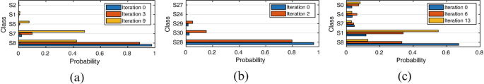
DNNs results: (a) Output probabilities for the Example 1 on the VGGNet: the blue bars represent the starting probabilities, the orange bars the probabilities at the point of misclassification, and the yellow bars at the DMAX. (b) Output probabilities for the Example 2 on the VGGNet: the blue bars represent the starting probabilities, and the orange bars the probabilities at the DMAX. (c) Output probabilities for the Example 1 on the LeNet: the blue bars represent the starting probabilities, the orange bars the probabilities at the point of misclassification, and the yellow bars at the DMAX
-
2.
The VGGNet classifies the input image (in Fig. 8d) as the “Children crossing” (S28) class with a probability equal to 0.96. The target class, which is “Beware of ice/snow” (S30), has a probability equal to 0.023. After 2 iterations, the distance overcomes DMAX = 250, while the VGGNet has not misclassified the image yet (see Fig. 8e). As in the previous example, this behavior is due to the high distance between the initial probabilities, as shown in Fig. 9b. Note that the VGGNet reaches DMAX in a lower number of iterations compared to the CapsNet.
-
3.
The LeNet classifies the input image (in Fig. 8a) as the “120 km/h speed limit” (S8) class with a probability equal to 0.672. The target class, which is “30 km/h speed limit” (S1), has a probability equal to 0.178. After 6 iterations, the LeNet is fooled, because the image (in Fig. 8f) is recognized as the target class with a probability equal to 0.339. The noise becomes perceptible after 13 iterations (Fig. 8g), where the distance overcomes DMAX = 520.


5.3 Discussion
While it is highly complex to formalize generic conclusions, a common trend is that the CapsNets are more robust against adversarial attacks and affine transformation than DNNs with similar depth and number of parameters. These observations are aligned with similar works of Michels et al. [58] and Gu et al. [25].
Concurrently, the CapsNets security has been analyzed from different perspectives. The Vote Attack [26] is a method that directly perturbs the CapsNets by manipulating the votes from primary capsules. Qin et al. [70] proposed a method to detect adversarial examples using the CapsNet reconstruction network.
These analyses and findings open several directions and strategies for deploying robust CapsNets in safety-critical applications.
6 Security for Spiking Neural Networks
SNNs are considered the third generation of neural networks [49] due to their high biological plausibility and similarities to the human brain. Compared to traditional DNNs, which are based on the computation of continuous values, SNNs process discrete spike trains in an event-based fashion. Hence, they exhibit great potential for deploying high-performance and energy-efficient ML algorithms [56, 90]. In terms of security, the different computational principles of SNNs offer unique vulnerabilities and potential optimizations for improving their robustness. In contrast to the well-established knowledge about DNN security, the robustness of SNNs is an ongoing research topic of high interest in the ML community.
6.1 Comparison DNNs vs. SNNs
The robustness evaluation of SNNs can be conducted by analyzing the comparison between an SNN and a (non-spiking) DNN having the same architectural model, i.e., the same number of layers, neurons per layer, and connections. While the DNN has traditional neurons with ReLU activation function, the SNN has LIF neurons with threshold voltage Vth = 1 V . For these experiments, we use a 5-layer network with 3 convolutional layers and 2 fully connected layers on the MNIST dataset [39]. The DNN is trained using the PyTorch framework [66], while the SNN has been implemented and trained with the Norse framework [68]. The PGD attack [50] is applied to both networks using the Foolbox library [73]. Figure 10 shows the accuracy results of both networks when varying the value of adversarial noise budget ε. While for low noise magnitude the DNN has slightly higher accuracy than the SNN, after the turnaround point of 0.5 ≤ ε ≤ 0.6, the opposite behavior is noticed. While the accuracy curve of the DNN decreases sharply, the SNN curve has a lower slope. For instance, when ε = 1, the SNN accuracy is more than 50% higher than the DNN accuracy [16]. Such an outcome indicates that SNNs have the potential to be applied in security contexts due to their higher inherent robustness compared to traditional DNNs. These findings are aligned with recent works [5, 37, 52, 80] that demonstrate the SNNs’ higher robustness against security threats, and motivate deeper analyses on this topic.

Comparison between a DNN and an SNN with the same structure under the PGD attack with different values of the adversarial perturbation ε (adapted from [16])
6.2 Improving the SNN Robustness Through Inherent Structural Parameters
The previous analyses can be extended not only by exploring the SNN robustness for different adversarial perturbations but also by studying the impact of the SNN structural parameters, i.e., spiking threshold voltage Vth and time window T. Vth represents the threshold to be compared with the spiking neuron’s membrane potential to decide whether or not to emit an output spike. T represents the observation period in which an SNN implemented with the rate-coding mechanism receives spike sequences associated with the same intensity value, which is associated with the firing rate.
6.2.1 SNN Robustness Exploration Methodology
Figure 11 shows the robustness exploration methodology, mainly composed of two steps:

Methodology for exploring the SNN robustness, varying the threshold voltage Vth, the time window T, and the adversarial perturbation ε [16]
-
1.
Learnability Analysis: Given the SNN architecture, the threshold voltage Vi, and the time window Tj, the training in the spiking domain is conducted. This step excludes the configurations of parameters that have low accuracy, by setting a minimum baseline accuracy level below which the SNN learning process is considered inefficient, since there is no interest in continuing the study on SNNs that do not converge.
-
2.
Security Analysis: For all the (Vi, Tj) tuples for which the SNN achieves high baseline accuracy, the security study is conducted. The adversarial examples are also generated based on the adversarial noise ε, and the SNN robustness is evaluated. The parameter ε models the strength of the attack, where a high value tends to reduce the SNN accuracy due to the higher perturbation budget given to the adversary. For every value of ε, the robustness is computed as the inverse of the attack’s success rate, i.e., how many adversarial examples are correctly classified by the SNN.
By observing the robust combinations of (Vi, Tj) during both the learnability and security analyses, a trustworthy SNN design is obtained at the output.
6.2.2 SNN Robustness Evaluation
The experiments were conducted using a 5-layer SNN similar to the LeNet-5 architecture adapted for the spiking domain. It is trained for the MNIST dataset [39] with the Norse framework [68], and the PGD adversarial attacks are implemented using the Foolbox library [73]. Figure 12a shows the heat map relative to the learnability analysis. The variations of Vth and T appear on the horizontal and vertical axes, respectively, while the color denotes the SNN accuracy. Compared to the default values, which are (Vi, Tj) = (1, 64), other combinations of parameters are explored and evaluated. While a high-accuracy region can be identified in the top-left corner (low Vi, high Tj), the accuracy is not monotonic w.r.t. both parameters, since the SNN with (Vi, Tj) = (1.25, 56) has lower accuracy than the surrounding points.

Heat maps showing the SNN accuracy for the MNIST dataset using different combinations of (Vi, Tj), based on the results in [16]. (a) Learnability analysis, equivalent of having ε = 0. (b) Security analysis, for ε = 1
Figure 12b show the security analysis heat map for ε = 1. A comparison between the two graphs indicates that high learnability (i.e., without adversarial attacks) does not guarantee high robustness. Indeed, different responses of the SNNs under adversarial attacks based on their respective structural parameters can be noticed. Two SNNs that have a comparable baseline accuracy may have different robustness. For example, the SNN with (Vi, Tj) = (0.75, 72) has 91% accuracy under attack, and the SNN with (Vi, Tj) = (0.5, 80) has only 27% accuracy, while their baseline accuracy is equal to 97% for both combinations.
Hence, studying the SNN security under different values of adversarial perturbations is crucial to identifying robust combinations of threshold voltage and time windows, which contribute to enabling the deployment of SNNs for safety-critical applications.
6.3 Adversarial Attacks and Defenses on Event-Based Data
Along with the efficient implementation of SNNs on neuromorphic architectures (e.g., Intel Loihi [15] and IBM TrueNorth [57]), other advancements in the vision field have come from the event-based camera sensor, such as the dynamic vision sensors (DVS) [41]. Unlike classical frame-based cameras, the DVS cameras emulate the behavior of the human retina by recording the information in the form of spike event sequences, which are generated each time a change of light intensity is detected. As a consequence, SNNs processing event-based data are affected by different types of security vulnerabilities compared to frame-based data processing.
Figure 13 provides an overview of the adversarial threat model used in this section. The frames of events recorded by a DVS camera are subjected to adversarial attacks, while DVS noise filters placed at the input of the neuromorphic hardware that executes SNN inference can mitigate the adversary perturbations.

Adversarial threat model for applying attack algorithms and noise filters on event-based SNNs. Figure adapted from [54]
6.3.1 Gradient-Based Attack for Event Sequences
There exist different types of adversarial attacks and noise filters specific to event-based data. A gradient-based attack [54], described in Algorithm 1, is an iterative algorithm that progressively updates the injected perturbations into the event sequences based on the loss function (lines 7–11 of Algorithm 1) for each frame series of the dataset. After defining a mask in which the perturbation should be added (line 7), the output probability and its respective loss, obtained in the presence of the perturbation, are computed in lines 9 and 10, respectively. Afterward, the perturbation values are updated based on the gradients of the inputs with respect to the loss.
Algorithm 1: Gradient-based adversarial attack methodology for event-based SNNs [54]

6.3.2 Background Activity Filter for Event Cameras
DVS sensors are mainly affected by noise caused by thermal noise and junction leakage current, which can be classified as a background activity. Since similar events are typically generated in a neighborhood of pixels, the real events have a higher spatio-temporal correlation than the noise events. Such empirical observation is exploited for generating the Background Activity Filter (BAF) [43, 53]. The spatio-temporal correlation between events is computed. If such correlation is lower than a certain threshold, the events are filtered out since they are likely due to noise, while the events with higher correlations are kept. The methodology is reported in Algorithm 2, where S and T are the parameters of the filter that set the dimensions of the spatio-temporal neighborhood. Large S and T values imply that few events are filtered out. The filter’s decision is based on the comparison between te − M[xe][ye] and T (lines 12–13 of Algorithm 2). The event is filtered out if the first term is lower.
Algorithm 2: Background activity filter for event sequences [53]

6.3.3 Evaluation of Gradient-Based Attack and Background Activity Filter
The experiments are conducted by training the 4-layer SNN described in [82], with two convolutional layers and two fully connected layers, for the DvsGesture dataset [4] using the SLAYER backpropagation method [82]. Figure 14 shows the results for the gradient-based attack applied to the SNN. When it is not protected by the BAF, the attack is successful since the SNN accuracy drops to 15.15%. However, the BAF plays the role of a suitable defense since the accuracy remains higher than 90% for a wide range of values for the parameters s and t. At the extremes, for t = 1, the accuracy is strongly affected by the parameter s, while for t = 500 the SNN accuracy drops to less than 48%.

Robustness evaluation for the SNN on the DvsGesture dataset, under the gradient-based attack and BAF filter. Based on the results in [54]
The results relative to a case study in which the gradient-based attack is applied to the sequence of events of a sample of the DvsGesture dataset are shown in Fig. 15. The first row (Fig. 15a) shows the results for the clean event sequence, i.e., without attack and without filter. The SNN correctly classifies the frame as the class 2, which corresponds to the “left hand wave” label. The second row (Fig. 15b) shows the outcome when the gradient-based adversarial attack is applied. The visible modifications in the event sequences are minimal, but the sample is misclassified by the SNN as the class 0, which corresponds to “hand clap.” The last row (Fig. 15c), relative to the scenario in which both the gradient-based attack and the BAF filter (with s = 2 and t = 5) are present, shows that the sequence is again correctly classified as the class 2 (“left hand wave”). It is worth noticing that several spurious events have been filtered out by the BAF, resulting in high SNN prediction confidence.

Detailed results of an event sequence of the DVSGesture dataset labeled as “left hand wave.” (a) Clean event sequence. (b) Event sequence under the gradient-based adversarial attack, unfiltered. (d) Event sequence under the gradient-based adversarial attack and protected by the BAF filter with s = 2 and t = 5. Based on the results in [54]
6.3.4 Dash Attack for Event Sequences
While the BAF filter is successful against the gradient-based attack, more sophisticated adversarial attack algorithms can evade this protection. For instance, the Dash Attack [53] injects events in the form of a dash. Only two pixels are perturbed for each time step. It starts by targeting the top-left corner (lines 11–13 of Algorithm 3). Afterward, the x and y coordinates are updated to hit only two consecutive pixels (see lines 17–25 of Algorithm 3). Hence, this attack results difficult to spot since the injected spikes do not cause a large overhead on the whole sample.
Algorithm 3: Dash attack methodology [53]

6.3.5 Mask Filter for Event Cameras
Another type of filtering methodology for event sequences is represented by the Mask Filter (MF) [43, 53]. Algorithm 4 shows the MF technique, whose basic functionality is to filter out the noise on the pixels which have low temporal contrast. The activity of each pixel coordinate is monitored (lines 10–11 of Algorithm 4). If such activity exceeds the temporal parameter T, the mask is activated (lines 14–15 of Algorithm 4). After setting all the pixel coordinates of the mask, each event corresponding to a coordinate in which the mask is active is filtered out (lines 15–16 of Algorithm 4).
Algorithm 4: Mask filter for event sequences [53]

6.3.6 Evaluation of the Dash Attack Against Background Activity Filter and Mask Filter
The Dash attack introduces perturbations that look very similar to the inherent background noise generated by the DVS camera recording the events. Therefore, they result difficult to be spotted. As shown in Fig. 16a, the accuracy of the SNN without filter under the Dash Attack drops to 0% for the DvsGesture dataset, while the BAF defense produces a slightly higher SNN accuracy. However, the accuracy peak of 28.41% achieved with the BAF with s = 1 and t = 10 is too low to consider the BAF as a good defense method against the Dash Attack. However, the MF represents a successful defense because the SNN accuracy is high for large values of T.

Evaluation of DVS attacks for the SNN on the DvsGesture dataset, under the BAF and Mask filters, based on the results in [53]. (a) Results for the Dash Attack. (b) Results for the MF-Aware Dash Attack
6.3.7 Mask Filter-Aware Dash Attack for Event Sequences
The main drawback of the Dash attack is its intrinsic weakness against the MF. In fact, it targets the same pixels for the complete sample duration. This highlights which pixels are targeted by the attack. Indeed, the number of events produced by the affected pixels is significantly higher than the events associated with the other pixel coordinates not hit by the attack. In addition, it mainly injects events on the boundaries of the images, which do not tend to overlap with useful information that is typically centered. Hence, by hitting the perimeter of the frames, there is a low risk of superimposing adversarial noise to the main subject. These observations explain the success of the MF in restoring the original SNN accuracy. The perturbed pixels are easily identifiable due to their high number of events, and the filter does not remove useful information, since the modifications are mainly conducted at the edge of the image. Based on these premises, the Mask Filter-Aware Dash Attack has been designed, aiming at being resistant to the MF. It receives as a parameter th that sets a limit on the number of frames that can be changed for each pixel (line 14 of Algorithm 5). Therefore, the algorithm hits a couple of pixels, as in the case of the Dash Attack. However, after injecting events into th frames, it moves to the following pixel coordinates (lines 17–19 of Algorithm 5). The visual effect created by the MF-Aware Dash Attack is that of a dash moving along a line. A smaller th implies a faster movement of the dash across the image.
Algorithm 5: Mask filter-aware dash attack methodology [53]

6.3.8 Evaluation of the Mask Filter-Aware Dash Attack Against Background Activity Filter and Mask Filter
Figure 16b shows the results relative to the experiments conducted for the MF-Aware Dash Attack, with different values of the parameter th. While the visibility of the injected noise on the DvsGesture dataset, reported for th = 150, is similar to the Dash Attacks, the behavior of the MF-Aware Dash Attack in the presence of noise filters is much different. The accuracy of the SNN under attack without filter is very low (up to 7.95% for th = 50. The SNN defended by the BAF shows discrete robustness, in particular, when s = 3 and t = 1. In such a scenario, the accuracy reaches 59.09% against the MF-Aware Dash Attack with th = 50. However, when t ≥ 5, the SNN accuracy is lower than 31.44%. The key advantage compared to the Dash Attack resides in the behavior of the MF-Aware Dash Attack in the presence of the MF. If T ≥ th, the SNN accuracy becomes lower than 23.5%. On the contrary, the behavior for T < th is similar to the results achieved for the Dash Attack. For example, the MF-Aware Dash Attack with th = 50 achieves 71.21% accuracy for T = 25, which is 20.83% lower than the original SNN accuracy. These results demonstrate that noise event filters such as the BAF and the MF significantly improve the SNN robustness against adversarial attacks. However, an adversarial attack algorithm specifically designed for being resistant to the MF, such as the MF-Aware Dash Attack, has the potential to break the noise filter defense for a good choice of its parameter th.
7 Conclusion
Despite being employed at a large scale, ML models are vulnerable to security threats. Therefore, several defensive mechanisms have been explored to increase their robustness. This chapter presented an overview of ML security, focusing on emerging architectures, such as DNNs, CapsNets, and SNNs. The high complexity of these models requires dedicated methodologies to investigate their trustworthiness. The analyses conducted in this chapter demonstrated that CapsNets are more robust than traditional DNNs against affine transformations and adversarial attacks. SNNs are inherently more robust than non-spiking DNNs, and such inherent robustness can be enhanced by fine-tuning their structural parameters, like the spiking voltage threshold and the time window. Moreover, event-based SNNs can be protected through noise filters for event sensors, like the Background Activity Filter and the Mask Filter. However, when properly tuned, advanced event-based adversarial attack methodologies, such as the Mask Filter-Aware Dash Attack, can cause significant accuracy drops in SNNs.
References
Abadi, M., Chu, A., Goodfellow, I.J., McMahan, H.B., Mironov, I., Talwar, K., Zhang, L.: Deep learning with differential privacy. In: Weippl, E.R., Katzenbeisser, S., Kruegel, C., Myers, A.C., Halevi, S. (eds.) Proceedings of the 2016 ACM SIGSAC Conference on Computer and Communications Security, Vienna, October 24–28, 2016, pp. 308–318. ACM, New York (2016). https://doi.org/10.1145/2976749.2978318
Agoyan, M., Dutertre, J., Mirbaha, A., Naccache, D., Ribotta, A., Tria, A.: How to flip a bit? In: 16th IEEE International On-line Testing Symposium (IOLTS 2010, 5–7 July, 2010, Corfu, pp. 235–239. IEEE Computer Society, Washington (2010). https://doi.org/10.1109/IOLTS.2010.5560194
Ali, H., Khalid, F., Tariq, H., Hanif, M.A., Ahmed, R., Rehman, S.: SSCNets: robustifying DNNs using secure selective convolutional filters. IEEE Des. Test 37(2), 58–65 (2020). https://doi.org/10.1109/MDAT.2019.2961325
Amir, A., Taba, B., Berg, D.J., Melano, T., McKinstry, J.L., di Nolfo, C., Nayak, T.K., Andreopoulos, A., Garreau, G., Mendoza, M., Kusnitz, J., DeBole, M., Esser, S.K., Delbrück, T., Flickner, M., Modha, D.S.: A low power, fully event-based gesture recognition system. In: 2017 IEEE Conference on Computer Vision and Pattern Recognition, CVPR 2017, Honolulu, July 21–26, 2017, pp. 7388–7397. IEEE Computer Society, Washington (2017). https://doi.org/10.1109/CVPR.2017.781
Bagheri, A., Simeone, O., Rajendran, B.: Adversarial training for probabilistic spiking neural networks. In: 19th IEEE International Workshop on Signal Processing Advances in Wireless Communications, SPAWC 2018, Kalamata, June 25–28, 2018, pp. 1–5. IEEE, Piscataway (2018). https://doi.org/10.1109/SPAWC.2018.8446003
Baumann, R.: Radiation-induced soft errors in advanced semiconductor technologies. IEEE Trans. Device Mater. Reliab. 5(3), 305–316 (2005). https://doi.org/10.1109/TDMR.2005.853449
Breier, J., Hou, X., Jap, D., Ma, L., Bhasin, S., Liu, Y.: Practical fault attack on deep neural networks. In: Lie, D., Mannan, M., Backes, M., Wang, X. (eds.) Proceedings of the 2018 ACM SIGSAC Conference on Computer and Communications Security, CCS 2018, Toronto, October 15–19, 2018, pp. 2204–2206. ACM, New York (2018). https://doi.org/10.1145/3243734.3278519
Brendel, W., Rauber, J., Bethge, M.: Decision-based adversarial attacks: reliable attacks against black-box machine learning models. In: 6th International Conference on Learning Representations, ICLR 2018, Vancouver, April 30–May 3, 2018. Conference Track Proceedings. OpenReview.net (2018). https://openreview.net/forum?id=SyZI0GWCZ
Capra, M., Bussolino, B., Marchisio, A., Masera, G., Martina, M., Shafique, M.: Hardware and software optimizations for accelerating deep neural networks: survey of current trends, challenges, and the road ahead. IEEE Access 8, 225134–225180 (2020). https://doi.org/10.1109/ACCESS.2020.3039858
Capra, M., Bussolino, B., Marchisio, A., Shafique, M., Masera, G., Martina, M.: An updated survey of efficient hardware architectures for accelerating deep convolutional neural networks. Fut. Int. 12(7), 113 (2020). https://doi.org/10.3390/fi12070113
Chen, Z., Li, G., Pattabiraman, K.: Ranger: boosting error resilience of deep neural networks through range restriction. CoRR abs/2003.13874 (2020). https://arxiv.org/abs/2003.13874
Clements, J., Lao, Y.: Hardware trojan design on neural networks. In: IEEE International Symposium on Circuits and Systems, ISCAS 2019, Sapporo, May 26–29, 2019, pp. 1–5. IEEE, Piscataway (2019). https://doi.org/10.1109/ISCAS.2019.8702493
Cohen, J.M., Rosenfeld, E., Kolter, J.Z.: Certified adversarial robustness via randomized smoothing. In: Chaudhuri, K., Salakhutdinov, R. (eds.) Proceedings of the 36th International Conference on Machine Learning, ICML 2019, 9–15 June 2019, Long Beach. Proceedings of Machine Learning Research, vol. 97, pp. 1310–1320. PMLR (2019). http://proceedings.mlr.press/v97/cohen19c.html
Dave, S., Marchisio, A., Hanif, M.A., Guesmi, A., Shrivastava, A., Alouani, I., Shafique, M.: Special session: towards an agile design methodology for efficient, reliable, and secure ML systems. In: 40th IEEE VLSI Test Symposium, VTS 2022, San Diego, April 25–27, 2022, pp. 1–14. IEEE, Piscataway (2022). https://doi.org/10.1109/VTS52500.2021.9794253
Davies, M., Srinivasa, N., Lin, T., Chinya, G.N., Cao, Y., Choday, S.H., Dimou, G.D., Joshi, P., Imam, N., Jain, S., Liao, Y., Lin, C., Lines, A., Liu, R., Mathaikutty, D., McCoy, S., Paul, A., Tse, J., Venkataramanan, G., Weng, Y., Wild, A., Yang, Y., Wang, H.: Loihi: A neuromorphic manycore processor with on-chip learning. IEEE Micro 38(1), 82–99 (2018). https://doi.org/10.1109/MM.2018.112130359
El-Allami, R., Marchisio, A., Shafique, M., Alouani, I.: Securing deep spiking neural networks against adversarial attacks through inherent structural parameters. In: Design, Automation & Test in Europe Conference & Exhibition, DATE 2021, Grenoble, February 1–5, 2021, pp. 774–779. IEEE, Piscataway (2021). https://doi.org/10.23919/DATE51398.2021.9473981
Eykholt, K., Evtimov, I., Fernandes, E., Li, B., Rahmati, A., Xiao, C., Prakash, A., Kohno, T., Song, D.: Robust physical-world attacks on deep learning visual classification. In: 2018 IEEE Conference on Computer Vision and Pattern Recognition, CVPR 2018, Salt Lake City, June 18–22, 2018, pp. 1625–1634. Computer Vision Foundation/IEEE Computer Society, Washington (2018). https://doi.org/10.1109/CVPR.2018.00175, http://openaccess.thecvf.com/content_cvpr_2018/html/Eykholt_Robust_Physical-World_Attacks_CVPR_2018_paper.html
Fani, R., Zamani, M.S.: Runtime hardware trojan detection by reconfigurable monitoring circuits. J. Supercomput. (2022). https://doi.org/10.1007/s11227-022-04362-1
Ganju, K., Wang, Q., Yang, W., Gunter, C.A., Borisov, N.: Property inference attacks on fully connected neural networks using permutation invariant representations. In: Lie, D., Mannan, M., Backes, M., Wang, X. (eds.) Proceedings of the 2018 ACM SIGSAC Conference on Computer and Communications Security, CCS 2018, Toronto, October 15–19, 2018, pp. 619–633. ACM, New York (2018). https://doi.org/10.1145/3243734.3243834
Gentry, C.: Fully homomorphic encryption using ideal lattices. In: Mitzenmacher, M. (ed.) Proceedings of the 41st Annual ACM Symposium on Theory of Computing, STOC 2009, Bethesda, May 31–June 2, 2009, pp. 169–178. ACM, New York (2009). https://doi.org/10.1145/1536414.1536440
Gilad-Bachrach, R., Dowlin, N., Laine, K., Lauter, K.E., Naehrig, M., Wernsing, J.: Cryptonets: applying neural networks to encrypted data with high throughput and accuracy. In: Balcan, M., Weinberger, K.Q. (eds.) Proceedings of the 33nd International Conference on Machine Learning, ICML 2016, New York City, June 19–24, 2016, JMLR Workshop and Conference Proceedings, vol. 48, pp. 201–210. JMLR.org (2016). http://proceedings.mlr.press/v48/gilad-bachrach16.html
Goodfellow, I.J., Pouget-Abadie, J., Mirza, M., Xu, B., Warde-Farley, D., Ozair, S., Courville, A.C., Bengio, Y.: Generative adversarial networks. CoRR abs/1406.2661 (2014). http://arxiv.org/abs/1406.2661
Goodfellow, I.J., Shlens, J., Szegedy, C.: Explaining and harnessing adversarial examples. In: Bengio, Y., LeCun, Y. (eds.) 3rd International Conference on Learning Representations, ICLR 2015, San Diego, May 7–9, 2015. Conference Track Proceedings (2015). http://arxiv.org/abs/1412.6572
Gu, T., Liu, K., Dolan-Gavitt, B., Garg, S.: BadNets: evaluating backdooring attacks on deep neural networks. IEEE Access 7, 47230–47244 (2019). https://doi.org/10.1109/ACCESS.2019.2909068
Gu, J., Tresp, V.: Improving the robustness of capsule networks to image affine transformations. In: 2020 IEEE/CVF Conference on Computer Vision and Pattern Recognition, CVPR 2020, Seattle, June 13–19, 2020, pp. 7283–7291. Computer Vision Foundation/IEEE, Piscataway (2020). https://doi.org/10.1109/CVPR42600.2020.00731, https://openaccess.thecvf.com/content_CVPR_2020/html/Gu_Improving_the_Robustness_of_Capsule_Networks_to_Image_Affine_Transformations_CVPR_2020_paper.html
Gu, J., Wu, B., Tresp, V.: Effective and efficient vote attack on capsule networks. In: 9th International Conference on Learning Representations, ICLR 2021, Virtual Event, May 3–7, 2021. OpenReview.net (2021). https://openreview.net/forum?id=33rtZ4Sjwjn
Guesmi, A., Alouani, I., Khasawneh, K.N., Baklouti, M., Frikha, T., Abid, M., Abu-Ghazaleh, N.B.: Defensive approximation: securing CNNs using approximate computing. In: Sherwood, T., Berger, E.D., Kozyrakis, C. (eds.) ASPLOS ’21: 26th ACM International Conference on Architectural Support for Programming Languages and Operating Systems, Virtual Event, April 19–23, 2021, pp. 990–1003. ACM, New York (2021). https://doi.org/10.1145/3445814.3446747
Hanif, M.A., Shafique, M.: Salvagednn: salvaging deep neural network accelerators with permanent faults through saliency-driven fault-aware mapping. Phil. Trans. R. Soc. A. 378(2164) (2020). https://doi.org/10.1098/rsta.2019.0164
Hanif, M.A., Shafique, M.: DNN-life: an energy-efficient aging mitigation framework for improving the lifetime of on-chip weight memories in deep neural network hardware architectures. In: Design, Automation & Test in Europe Conference & Exhibition, DATE 2021, Grenoble, February 1–5, 2021, pp. 729–734. IEEE, Piscataway (2021). https://doi.org/10.23919/DATE51398.2021.9473943
Hoang, L.H., Hanif, M.A., Shafique, M.: FT-ClipAct: resilience analysis of deep neural networks and improving their fault tolerance using clipped activation. In: 2020 Design, Automation & Test in Europe Conference & Exhibition, DATE 2020, Grenoble, March 9–13, 2020, pp. 1241–1246. IEEE, Piscataway (2020). https://doi.org/10.23919/DATE48585.2020.9116571
Juvekar, C., Vaikuntanathan, V., Chandrakasan, A.P.: GAZELLE: a low latency framework for secure neural network inference. In: Enck, W., Felt, A.P. (eds.) 27th USENIX Security Symposium, USENIX Security 2018, Baltimore, August 15–17, 2018, pp. 1651–1669. USENIX Association, Berkeley (2018). https://www.usenix.org/conference/usenixsecurity18/presentation/juvekar
Kang, K., Gangwal, S., Park, S.P., Roy, K.: NBTI induced performance degradation in logic and memory circuits: how effectively can we approach a reliability solution? In: Kyung, C., Choi, K., Ha, S. (eds.) Proceedings of the 13th Asia South Pacific Design Automation Conference, ASP-DAC 2008, Seoul, January 21–24, 2008, pp. 726–731. IEEE, Piscataway (2008). https://doi.org/10.1109/ASPDAC.2008.4484047
Khalid, F., Ali, H., Tariq, H., Hanif, M.A., Rehman, S., Ahmed, R., Shafique, M.: QuSecNets: quantization-based defense mechanism for securing deep neural network against adversarial attacks. In: Gizopoulos, D., Alexandrescu, D., Papavramidou, P., Maniatakos, M. (eds.) 25th IEEE International Symposium on On-Line Testing and Robust System Design, IOLTS 2019, Rhodes, July 1–3, 2019, pp. 182–187. IEEE, Piscataway (2019). https://doi.org/10.1109/IOLTS.2019.8854377
Khalid, F., Ali, H., Hanif, M.A., Rehman, S., Ahmed, R., Shafique, M.: FaDec: a fast decision-based attack for adversarial machine learning. In: 2020 International Joint Conference on Neural Networks, IJCNN 2020, Glasgow, July 19–24, 2020, pp. 1–8. IEEE, Piscataway (2020). https://doi.org/10.1109/IJCNN48605.2020.9207635
Kim, Y., Daly, R., Kim, J.S., Fallin, C., Lee, J., Lee, D., Wilkerson, C., Lai, K., Mutlu, O.: Flipping bits in memory without accessing them: an experimental study of DRAM disturbance errors. In: ACM/IEEE 41st International Symposium on Computer Architecture, ISCA 2014, Minneapolis, June 14–18, 2014, pp. 361–372. IEEE Computer Society, Washington (2014). https://doi.org/10.1109/ISCA.2014.6853210
Kumar, A.D.: Novel deep learning model for traffic sign detection using capsule networks. CoRR abs/1805.04424 (2018). http://arxiv.org/abs/1805.04424
Kundu, S., Pedram, M., Beerel, P.A.: HIRE-SNN: harnessing the inherent robustness of energy-efficient deep spiking neural networks by training with crafted input noise. In: 2021 IEEE/CVF International Conference on Computer Vision, ICCV 2021, Montreal, October 10–17, 2021, pp. 5189–5198. IEEE, Piscataway (2021). https://doi.org/10.1109/ICCV48922.2021.00516
Kurakin, A., Goodfellow, I.J., Bengio, S.: Adversarial examples in the physical world. In: 5th International Conference on Learning Representations, ICLR 2017, Toulon, April 24–26, 2017, Workshop Track Proceedings. OpenReview.net (2017). https://openreview.net/forum?id=HJGU3Rodl
LeCun, Y., Bottou, L., Bengio, Y., Haffner, P.: Gradient-based learning applied to document recognition. Proc. IEEE 86(11), 2278–2324 (1998). https://doi.org/10.1109/5.726791
Li, J., Rakin, A.S., Xiong, Y., Chang, L., He, Z., Fan, D., Chakrabarti, C.: Defending bit-flip attack through DNN weight reconstruction. In: 57th ACM/IEEE Design Automation Conference, DAC 2020, San Francisco, July 20–24, 2020, pp. 1–6. IEEE, Piscataway (2020). https://doi.org/10.1109/DAC18072.2020.9218665
Lichtsteiner, P., Posch, C., Delbrück, T.: A 128×128 120 dB 15 μs latency asynchronous temporal contrast vision sensor. IEEE J. Solid State Circuits 43(2), 566–576 (2008). https://doi.org/10.1109/JSSC.2007.914337
Lin, J., Gan, C., Han, S.: Defensive quantization: When efficiency meets robustness. In: 7th International Conference on Learning Representations, ICLR 2019, New Orleans, May 6–9, 2019. OpenReview.net (2019). https://openreview.net/forum?id=ryetZ20ctX
Linares-Barranco, A., Perez-Peña, F., Moeys, D.P., Gomez-Rodriguez, F., Jiménez-Moreno, G., Liu, S., Delbrück, T.: Low latency event-based filtering and feature extraction for dynamic vision sensors in real-time FPGA applications. IEEE Access 7, 134926–134942 (2019). https://doi.org/10.1109/ACCESS.2019.2941282
Liu, J., Juuti, M., Lu, Y., Asokan, N.: Oblivious neural network predictions via MiniONN transformations. In: Thuraisingham, B.M., Evans, D., Malkin, T., Xu, D. (eds.) Proceedings of the 2017 ACM SIGSAC Conference on Computer and Communications Security, CCS 2017, Dallas, October 30–November 03, 2017, pp. 619–631. ACM, New York (2017). https://doi.org/10.1145/3133956.3134056
Liu, Y., Wei, L., Luo, B., Xu, Q.: Fault injection attack on deep neural network. In: Parameswaran, S. (ed.) 2017 IEEE/ACM International Conference on Computer-Aided Design, ICCAD 2017, Irvine, November 13–16, 2017, pp. 131–138. IEEE, Piscataway (2017). https://doi.org/10.1109/ICCAD.2017.8203770
Liu, K., Dolan-Gavitt, B., Garg, S.: Fine-pruning: defending against backdooring attacks on deep neural networks. In: Bailey, M., Holz, T., Stamatogiannakis, M., Ioannidis, S. (eds.) Research in Attacks, Intrusions, and Defenses – 21st International Symposium, RAID 2018, Heraklion, Crete, September 10–12, 2018, Proceedings, Lecture Notes in Computer Science, vol. 11050, pp. 273–294. Springer, Berlin (2018). https://doi.org/10.1007/978-3-030-00470-5_13
Liu, X., Deng, R.H., Wu, P., Yang, Y.: Lightning-fast and privacy-preserving outsourced computation in the cloud. Cybersecur 3(1), 17 (2020). https://doi.org/10.1186/s42400-020-00057-3
Lyons, R.E., Vanderkulk, W.: The use of triple-modular redundancy to improve computer reliability. IBM J. Res. Dev. 6(2), 200–209 (1962). https://doi.org/10.1147/rd.62.0200
Maass, W.: Networks of spiking neurons: the third generation of neural network models. Neural Netw. 10(9), 1659–1671 (1997). https://doi.org/10.1016/S0893-6080(97)00011-7
Madry, A., Makelov, A., Schmidt, L., Tsipras, D., Vladu, A.: Towards deep learning models resistant to adversarial attacks. In: 6th International Conference on Learning Representations, ICLR 2018, Vancouver, April 30–May 3, 2018, Conference Track Proceedings. OpenReview.net (2018). https://openreview.net/forum?id=rJzIBfZAb
Marchisio, A., Nanfa, G., Khalid, F., Hanif, M.A., Martina, M., Shafique, M.: CapsAttacks: robust and imperceptible adversarial attacks on capsule networks. CoRR abs/1901.09878 (2019). http://arxiv.org/abs/1901.09878
Marchisio, A., Nanfa, G., Khalid, F., Hanif, M.A., Martina, M., Shafique, M.: Is spiking secure? A comparative study on the security vulnerabilities of spiking and deep neural networks. In: 2020 International Joint Conference on Neural Networks, IJCNN 2020, Glasgow, July 19–24, 2020, pp. 1–8. IEEE, Piscataway (2020). https://doi.org/10.1109/IJCNN48605.2020.9207297
Marchisio, A., Pira, G., Martina, M., Masera, G., Shafique, M.: DVS-attacks: adversarial attacks on dynamic vision sensors for spiking neural networks. In: International Joint Conference on Neural Networks, IJCNN 2021, Shenzhen, July 18–22, 2021, pp. 1–9. IEEE, Piscataway (2021). https://doi.org/10.1109/IJCNN52387.2021.9534364
Marchisio, A., Pira, G., Martina, M., Masera, G., Shafique, M.: R-SNN: an analysis and design methodology for robustifying spiking neural networks against adversarial attacks through noise filters for dynamic vision sensors. In: IEEE/RSJ International Conference on Intelligent Robots and Systems, IROS 2021, Prague, September 27–Oct. 1, 2021, pp. 6315–6321. IEEE, Piscataway (2021). https://doi.org/10.1109/IROS51168.2021.9636718
Marchisio, A., Caramia, G., Martina, M., Shafique, M.: fakeWeather: adversarial attacks for deep neural networks emulating weather conditions on the camera lens of autonomous systems. In: 2022 International Joint Conference on Neural Networks, IJCNN 2022, Padua, July 18–23, 2022. IEEE, Piscataway (2022)
Massa, R., Marchisio, A., Martina, M., Shafique, M.: An efficient spiking neural network for recognizing gestures with a DVS camera on the Loihi neuromorphic processor. In: 2020 International Joint Conference on Neural Networks, IJCNN 2020, Glasgow, July 19–24, 2020, pp. 1–9. IEEE, Piscataway (2020). https://doi.org/10.1109/IJCNN48605.2020.9207109
Merolla, P.A., Arthur, J.V., Alvarez-Icaza, R., Cassidy, A.S., Sawada, J., Akopyan, F., Jackson, B.L., Imam, N., Guo, C., Nakamura, Y., Brezzo, B., Vo, I., Esser, S.K., Appuswamy, R., Taba, B., Amir, A., Flickner, M.D., Risk, W.P., Manohar, R., Modha, D.S.: A million spiking-neuron integrated circuit with a scalable communication network and interface. Science 345(6197), 668–673 (2014). https://doi.org/10.1126/science.1254642, https://www.science.org/doi/abs/10.1126/science.1254642
Michels, F., Uelwer, T., Upschulte, E., Harmeling, S.: On the vulnerability of capsule networks to adversarial attacks. CoRR abs/1906.03612 (2019). http://arxiv.org/abs/1906.03612
Mohassel, P., Zhang, Y.: SecureML: a system for scalable privacy-preserving machine learning. In: 2017 IEEE Symposium on Security and Privacy, SP 2017, San Jose, May 22–26, 2017, pp. 19–38. IEEE Computer Society, Washington (2017). https://doi.org/10.1109/SP.2017.12
Nandakumar, K., Ratha, N.K., Pankanti, S., Halevi, S.: Towards deep neural network training on encrypted data. In: IEEE Conference on Computer Vision and Pattern Recognition Workshops, CVPR Workshops 2019, Long Beach, June 16–20, 2019, pp. 40–48. Computer Vision Foundation/IEEE, Piscataway (2019). https://doi.org/10.1109/CVPRW.2019.00011, http://openaccess.thecvf.com/content_CVPRW_2019/html/CV-COPS/Nandakumar_Towards_Deep_Neural_Network_Training_on_Encrypted_Data_CVPRW_2019_paper.html
Ozen, E., Orailoglu, A.: Sanity-check: Boosting the reliability of safety-critical deep neural network applications. In: 28th IEEE Asian Test Symposium, ATS 2019, Kolkata, December 10–13, 2019, pp. 7–12. IEEE, Piscataway (2019). https://doi.org/10.1109/ATS47505.2019.000-8
Ozen, E., Orailoglu, A.: Boosting bit-error resilience of DNN accelerators through median feature selection. IEEE Trans. Comput. Aided Des. Integr. Circuits Syst. 39(11), 3250–3262 (2020). https://doi.org/10.1109/TCAD.2020.3012209
Paillier, P.: Public-key cryptosystems based on composite degree residuosity classes. In: Stern, J. (ed.) Advances in Cryptology – EUROCRYPT ’99, Proceeding of the International Conference on the Theory and Application of Cryptographic Techniques, Prague, May 2–6, 1999. Lecture Notes in Computer Science, vol. 1592, pp. 223–238. Springer, Berlin (1999). https://doi.org/10.1007/3-540-48910-X_16
Pandey, P., Basu, P., Chakraborty, K., Roy, S.: GreenTPU: predictive design paradigm for improving timing error resilience of a near-threshold tensor processing unit. IEEE Trans. Very Large Scale Integr. Syst. 28(7), 1557–1566 (2020). https://doi.org/10.1109/TVLSI.2020.2985057
Papernot, N., Song, S., Mironov, I., Raghunathan, A., Talwar, K., Erlingsson, Ú.: Scalable private learning with PATE. In: 6th International Conference on Learning Representations, ICLR 2018, Vancouver, April 30–May 3, 2018. Conference Track Proceedings. OpenReview.net (2018). https://openreview.net/forum?id=rkZB1XbRZ
Paszke, A., Gross, S., Massa, F., Lerer, A., Bradbury, J., Chanan, G., Killeen, T., Lin, Z., Gimelshein, N., Antiga, L., Desmaison, A., Köpf, A., Yang, E.Z., DeVito, Z., Raison, M., Tejani, A., Chilamkurthy, S., Steiner, B., Fang, L., Bai, J., Chintala, S.: PyTorch: An imperative style, high-performance deep learning library. In: Wallach, H.M., Larochelle, H., Beygelzimer, A., d’Alché-Buc, F., Fox, E.B., Garnett, R. (eds.) Advances in Neural Information Processing Systems 32: Annual Conference on Neural Information Processing Systems 2019, NeurIPS 2019, December 8–14, 2019, Vancouver, pp. 8024–8035 (2019). https://proceedings.neurips.cc/paper/2019/hash/bdbca288fee7f92f2bfa9f7012727740-Abstract.html
Paudice, A., Muñoz-González, L., György, A., Lupu, E.C.: Detection of adversarial training examples in poisoning attacks through anomaly detection. CoRR abs/1802.03041 (2018). http://arxiv.org/abs/1802.03041
Pehle, C., Pedersen, J.E.: Norse—a deep learning library for spiking neural networks (2021). https://doi.org/10.5281/zenodo.4422025. Documentation: https://norse.ai/docs/
Prasanth, V., Singh, V., Parekhji, R.A.: Reduced overhead soft error mitigation using error control coding techniques. In: 17th IEEE International On-line Testing Symposium (IOLTS 2011), 13–15 July, 2011, Athens, pp. 163–168. IEEE Computer Society, Washington (2011). https://doi.org/10.1109/IOLTS.2011.5993831
Qin, Y., Frosst, N., Sabour, S., Raffel, C., Cottrell, G.W., Hinton, G.E.: Detecting and diagnosing adversarial images with class-conditional capsule reconstructions. In: 8th International Conference on Learning Representations, ICLR 2020, Addis Ababa, April 26–30, 2020. OpenReview.net (2020). https://openreview.net/forum?id=Skgy464Kvr
Raghunathan, B., Turakhia, Y., Garg, S., Marculescu, D.: Cherry-picking: exploiting process variations in dark-silicon homogeneous chip multi-processors. In: Macii, E. (ed.) Design, Automation and Test in Europe, DATE 13, Grenoble, March 18–22, 2013, pp. 39–44. EDA Consortium San Jose/ACM DL, New York (2013). https://doi.org/10.7873/DATE.2013.023
Rakin, A.S., He, Z., Fan, D.: Bit-flip attack: Crushing neural network with progressive bit search. In: 2019 IEEE/CVF International Conference on Computer Vision, ICCV 2019, Seoul, October 27–November 2, 2019, pp. 1211–1220. IEEE, Piscataway (2019). https://doi.org/10.1109/ICCV.2019.00130
Rauber, J., Brendel, W., Bethge, M.: Foolbox v0.8.0: a python toolbox to benchmark the robustness of machine learning models. CoRR abs/1707.04131 (2017). http://arxiv.org/abs/1707.04131
Rouhani, B.D., Riazi, M.S., Koushanfar, F.: DeepSecure: scalable provably-secure deep learning. In: Proceedings of the 55th Annual Design Automation Conference, DAC 2018, San Francisco, June 24–29, 2018, pp. 2:1–2:6. ACM, New York (2018). https://doi.org/10.1145/3195970.3196023
Sabour, S., Frosst, N., Hinton, G.E.: Dynamic routing between capsules. In: Guyon, I., von Luxburg, U., Bengio, S., Wallach, H.M., Fergus, R., Vishwanathan, S.V.N., Garnett, R. (eds.) Advances in Neural Information Processing Systems 30: Annual Conference on Neural Information Processing Systems 2017, December 4–9, 2017, Long Beach, pp. 3856–3866 (2017). https://proceedings.neurips.cc/paper/2017/hash/2cad8fa47bbef282badbb8de5374b894-Abstract.html
Shafahi, A., Huang, W.R., Najibi, M., Suciu, O., Studer, C., Dumitras, T., Goldstein, T.: Poison frogs! targeted clean-label poisoning attacks on neural networks. In: Bengio, S., Wallach, H.M., Larochelle, H., Grauman, K., Cesa-Bianchi, N., Garnett, R. (eds.) Advances in Neural Information Processing Systems 31: Annual Conference on Neural Information Processing Systems 2018, NeurIPS 2018, December 3–8, 2018, Montréal, pp. 6106–6116 (2018). https://proceedings.neurips.cc/paper/2018/hash/22722a343513ed45f14905eb07621686-Abstract.html
Shafique, M., Naseer, M., Theocharides, T., Kyrkou, C., Mutlu, O., Orosa, L., Choi, J.: Robust machine learning systems: challenges, current trends, perspectives, and the road ahead. IEEE Des. Test 37(2), 30–57 (2020). https://doi.org/10.1109/MDAT.2020.2971217
Shafique, M., Marchisio, A., Putra, R.V.W., Hanif, M.A.: Towards energy-efficient and secure edge AI: a cross-layer framework ICCAD special session paper. In: IEEE/ACM International Conference On Computer Aided Design, ICCAD 2021, Munich, November 1–4, 2021, pp. 1–9. IEEE, Piscataway (2021). https://doi.org/10.1109/ICCAD51958.2021.9643539
Sharif, M., Bhagavatula, S., Bauer, L., Reiter, M.K.: Accessorize to a crime: real and stealthy attacks on state-of-the-art face recognition. In: Weippl, E.R., Katzenbeisser, S., Kruegel, C., Myers, A.C., Halevi, S. (eds.) Proceedings of the 2016 ACM SIGSAC Conference on Computer and Communications Security, Vienna, October 24–28, 2016, pp. 1528–1540. ACM, New York (2016). https://doi.org/10.1145/2976749.2978392
Sharmin, S., Rathi, N., Panda, P., Roy, K.: Inherent adversarial robustness of deep spiking neural networks: Effects of discrete input encoding and non-linear activations. In: Vedaldi, A., Bischof, H., Brox, T., Frahm, J. (eds.) Proceedings of the Computer Vision – ECCV 2020 – 16th European Conference, Glasgow, August 23–28, 2020, Part XXIX. Lecture Notes in Computer Science, vol. 12374, pp. 399–414. Springer, Berlin (2020). https://doi.org/10.1007/978-3-030-58526-6_24
Shokri, R., Stronati, M., Song, C., Shmatikov, V.: Membership inference attacks against machine learning models. In: 2017 IEEE Symposium on Security and Privacy, SP 2017, San Jose, May 22–26, 2017, pp. 3–18. IEEE Computer Society, Washington (2017). https://doi.org/10.1109/SP.2017.41
Shrestha, S.B., Orchard, G.: SLAYER: spike layer error reassignment in time. In: Bengio, S., Wallach, H.M., Larochelle, H., Grauman, K., Cesa-Bianchi, N., Garnett, R. (eds.) Advances in Neural Information Processing Systems 31: Annual Conference on Neural Information Processing Systems 2018, NeurIPS 2018, December 3–8, 2018, Montréal, pp. 1419–1428 (2018). https://proceedings.neurips.cc/paper/2018/hash/82f2b308c3b01637c607ce05f52a2fed-Abstract.html
Siddique, A., Hoque, K.A.: Is approximation universally defensive against adversarial attacks in deep neural networks? CoRR abs/2112.01555 (2021). https://arxiv.org/abs/2112.01555
Stallkamp, J., Schlipsing, M., Salmen, J., Igel, C.: The German traffic sign recognition benchmark: a multi-class classification competition. In: The 2011 International Joint Conference on Neural Networks, IJCNN 2011, San Jose, July 31–August 5, 2011, pp. 1453–1460. IEEE, Piscataway (2011). https://doi.org/10.1109/IJCNN.2011.6033395
Su, J., Vargas, D.V., Sakurai, K.: One pixel attack for fooling deep neural networks. IEEE Trans. Evol. Comput. 23(5), 828–841 (2019). https://doi.org/10.1109/TEVC.2019.2890858
Thys, S., Ranst, W.V., Goedemé, T.: Fooling automated surveillance cameras: adversarial patches to attack person detection. In: IEEE Conference on Computer Vision and Pattern Recognition Workshops, CVPR Workshops 2019, Long Beach, June 16–20, 2019, pp. 49–55. Computer Vision Foundation/IEEE, Piscataway (2019). https://doi.org/10.1109/CVPRW.2019.00012, http://openaccess.thecvf.com/content_CVPRW_2019/html/CV-COPS/Thys_Fooling_Automated_Surveillance_Cameras_Adversarial_Patches_to_Attack_Person_Detection_CVPRW_2019_paper.html
Tramèr, F., Zhang, F., Juels, A., Reiter, M.K., Ristenpart, T.: Stealing machine learning models via prediction APIs. In: Holz, T., Savage, S. (eds.) 25th USENIX Security Symposium, USENIX Security 16, Austin, August 10–12, 2016, pp. 601–618. USENIX Association, Berkeley (2016). https://www.usenix.org/conference/usenixsecurity16/technical-sessions/presentation/tramer
Vadlamani, R., Zhao, J., Burleson, W.P., Tessier, R.: Multicore soft error rate stabilization using adaptive dual modular redundancy. In: Micheli, G.D., Al-Hashimi, B.M., Müller, W., Macii, E. (eds.) Design, Automation and Test in Europe, DATE 2010, Dresden, March 8–12, 2010, pp. 27–32. IEEE Computer Society, Washington (2010). https://doi.org/10.1109/DATE.2010.5457242
Venceslai, V., Marchisio, A., Alouani, I., Martina, M., Shafique, M.: NeuroAttack: undermining spiking neural networks security through externally triggered bit-flips. In: 2020 International Joint Conference on Neural Networks, IJCNN 2020, Glasgow, July 19–24, 2020, pp. 1–8. IEEE, Piscataway (2020). https://doi.org/10.1109/IJCNN48605.2020.9207351
Viale, A., Marchisio, A., Martina, M., Masera, G., Shafique, M.: Carsnn: An efficient spiking neural network for event-based autonomous cars on the Loihi neuromorphic research processor. In: International Joint Conference on Neural Networks, IJCNN 2021, Shenzhen, July 18–22, 2021, pp. 1–10. IEEE, Piscataway (2021). https://doi.org/10.1109/IJCNN52387.2021.9533738
Wagh, S., Gupta, D., Chandran, N.: SecureNN: 3-party secure computation for neural network training. Proc. Priv. Enhancing Technol. 2019(3), 26–49 (2019). https://doi.org/10.2478/popets-2019-0035
Wang, B., Gong, N.Z.: Stealing hyperparameters in machine learning. In: Proceedings of the 2018 IEEE Symposium on Security and Privacy, SP 2018, 21–23 May 2018, San Francisco, pp. 36–52. IEEE Computer Society, Washington (2018). https://doi.org/10.1109/SP.2018.00038
Wang, L., Guo, S., Huang, W., Qiao, Y.: Places205-vggnet models for scene recognition. CoRR abs/1508.01667 (2015). http://arxiv.org/abs/1508.01667
Zhang, J., Rangineni, K., Ghodsi, Z., Garg, S.: ThunderVolt: enabling aggressive voltage underscaling and timing error resilience for energy efficient deep learning accelerators. In: Proceedings of the 55th Annual Design Automation Conference, DAC 2018, San Francisco, June 24–29, 2018, pp. 19:1–19:6. ACM, New York (2018). https://doi.org/10.1145/3195970.3196129
Zhang, J.J., Gu, T., Basu, K., Garg, S.: Analyzing and mitigating the impact of permanent faults on a systolic array based neural network accelerator. In: 36th IEEE VLSI Test Symposium, VTS 2018, San Francisco, April 22–25, 2018, pp. 1–6. IEEE Computer Society, Washington (2018). https://doi.org/10.1109/VTS.2018.8368656
Zhang, J.J., Liu, K., Khalid, F., Hanif, M.A., Rehman, S., Theocharides, T., Artussi, A., Shafique, M., Garg, S.: Building robust machine learning systems: current progress, research challenges, and opportunities. In: Proceedings of the 56th Annual Design Automation Conference 2019, DAC 2019, Las Vegas, June 02–06, 2019, p. 175. ACM, New York (2019). https://doi.org/10.1145/3316781.3323472
Zhao, K., Di, S., Li, S., Liang, X., Zhai, Y., Chen, J., Ouyang, K., Cappello, F., Chen, Z.: FT-CNN: algorithm-based fault tolerance for convolutional neural networks. IEEE Trans. Parallel Distrib. Syst. 32(7), 1677–1689 (2021). https://doi.org/10.1109/TPDS.2020.3043449
Acknowledgements
This work has been supported in part by Intel Corporation through Gift funding for the project “Cost-Effective Dependability for Deep Neural Networks and Spiking Neural Networks,” and in part by the Doctoral College Resilient Embedded Systems, which is run jointly by the TU Wien’s Faculty of Informatics and the UAS Technikum Wien. This work was also supported in parts by the NYUAD Center for Interacting Urban Networks (CITIES), funded by Tamkeen under the NYUAD Research Institute Award CG001, Center for CyberSecurity (CCS), funded by Tamkeen under the NYUAD Research Institute Award G1104, and Center for Artificial Intelligence and Robotics (CAIR), funded by Tamkeen under the NYUAD Research Institute Award CG010.
Author information
Authors and Affiliations
Corresponding author
Editor information
Editors and Affiliations
Rights and permissions
Copyright information
© 2024 The Author(s), under exclusive license to Springer Nature Switzerland AG
About this chapter

Cite this chapter
Marchisio, A., Hanif, M.A., Shafique, M. (2024). Adversarial ML for DNNs, CapsNets, and SNNs at the Edge. In: Pasricha, S., Shafique, M. (eds) Embedded Machine Learning for Cyber-Physical, IoT, and Edge Computing. Springer, Cham. https://doi.org/10.1007/978-3-031-40677-5_18
Download citation
DOI: https://doi.org/10.1007/978-3-031-40677-5_18
Published:
Publisher Name: Springer, Cham
Print ISBN: 978-3-031-40676-8
Online ISBN: 978-3-031-40677-5
eBook Packages: EngineeringEngineering (R0)