Jet Schemes and Their Applications in Singularities, Toric Resolutions and Integer Partitions

Abstract

After a brief introduction to jet schemes, this article surveys their applications in singularity theory (Nash problem, motivic integration, birational geometry, jet components graph, equisingularity, local algebras of arc spaces), in the search for toric resolution of singularities (Teissier’s conjecture) and in the theory of integer partitions.

Dedicated to Monique Lejeune-Jalabert

4.1 Introduction

There exist in the literature several surveys of various aspects of jet schemes and arc spaces. This paper is meant on one hand to show the diversity of these aspects and guide the reader through it and on the other hand to survey some other aspects which do not appear in the existing surveys. First, let us say what intuitively are the jet schemes and the arc space of a variety X defined over a field $\mathbf {K}.$ The arc space of X is the scheme (or the infinite dimensional variety) $X_\infty$ which parametrizes the germs of formal curves (arcs) traced on $X;$i.e.,, a point on $X_\infty$ corresponds to an arc traced on $X.$ The jet schemes are finite dimensional approximations of the arc space: If we consider X embedded in an affine space, $X\subset {\mathbf {A}}^n,$ for $m\in {\mathbb N},$ the m-th jet scheme $X_m$ can be thought (modulo a trivial fibration) as the space of arcs in the ambient space ${\mathbf {A}}^n$ which have “contact” with X larger than $m.$

The arc space and the jet schemes ofXare rather complicated compared toX: the arc space is in general infinite dimensional; the jet schemes have in general many irreducible components of different dimensions; they are in general not reduced …but one can formulate the guiding philosophy of this article as follows: arc spaces and jet schemes can transform a difficult problem concerning a relatively simple object into a relatively simple problem concerning a difficult object.

Maybe one of the first uses of arc spaces in singularity theory goes back to Nash and is “subsequent” (1968) to the proof of existence of resolution of singularities by Hironaka. One can realize easily, that if there exists a resolution of singularities $\mu :Z\longrightarrow X,$ then X admits infinitely many other resolutions, an infinite family of them is obtained by blowing up Z along regular loci. Nash wanted to codify the data which is common to all these resolutions of singularities. He suggested that this data is hidden in the arc space ; a precise form of this suggestion is what is nowadays known as the Nash problem, but also the generalized Nash problem, or the embedded Nash problem which are generalizations of the first problem. In Sect. 4.3, we will briefly discuss these problems which have made fantastic progress in the last decade.

Another momentum was the introduction of the (geometric) motivic integration (Kontsevich, Denef-Loeser) in analogy with $p-$adic integration. The arc space of a variety is the measured space in this theory; the name motivic is related to the value that takes a motivic integral, which is an element in the “Grothendieck ring” (i.e., a class of a geometric object) and not a real number. This theory led to the introduction, again sometimes in analogy with $p-$adic integration but not only, of several new (motivic) invariants of singularities; this also led to another “stronger version” of the monodromy conjecture. This will be mentioned in Sect. 4.4.

The development of the geometric tools needed for motivic integration (which in particular allowed to prove the change of variables formula) led to a very effective use of jet schemes and arc spaces in the minimal model program and in “hunting” invariants of singularities of pairs (Mustaţă, Ein, Yasuda,…). This will be highlighted in Sect. 4.5.

Section 4.6 is dedicated to a weighted graph (the jet components graph) which was introduced by the author and which encodes the geometry of the jet schemes of the singularity and their truncation maps (these maps will be introduced in Sect. 4.2). We will mention some results about the structure of this graph (and hence the structure of the jet schemes) for several classes of singularities. For instance the data of this graph for irreducible plane branches, for two dimensional quasi-ordinary hypersurfaces (with H. Cobo), or for normal toric singularities is equivalent to the data of the embedded topological type of these singularities. This graph is actually determined by the irreducible components of the jet schemes, their dimensions and embedding dimensions and their behaviour with respect to the truncation maps; in particular this graph is determined by basic invariants of the jet schemes, but we can extract from it a complete invariant of the embedded topological type for these classes of singularities; the topological type is a very fine invariant of singularities. This reflects the philosophy that we mentioned above.

Section 4.7 describes how jet schemes intervene in an approach of the author to the problem of construction of embedded resolutions of singularities. This approach can be thought as a reverse Nash problem and is at the same time an approach to Teissier’s conjecture on resolution of singularities with toric morphisms.

Section 4.8 concerns an equisingularity theory (Leyton-Alvarez) which is based on deformations of jet schemes, and comparisons with other equisingularity theories. This problem generalizes the study of the jet schemes of irreducible plane curves in an equisingular family which was considered by the author.

Section 4.9 describes a link (Bruschek, Mourtada, Schepers) between some aspects of classical number theory, namely the study of integer partitions and singularity theory via arc spaces. The main object of this link (the Arc Hilbert-Poincaré series) makes use of the cone structure of the arc space.

Section 4.10 concerns the structure of the localization of the algebra of arcs at two types of points (arcs): On one hand rational points (Drinfeld, Grinberg, Kazhdan) and the invariants of singularities which can be extracted of this structure (Bourqui, Sebag) and on the other hand stable points or points associated with divisorial valuations (Reguera, Mourtada-Reguera).

4.2 The Construction of Jet Schemes

Let $\mathbf {K}$ be an algebraically closed field and X an algebraic variety defined over $\mathbf {K}.$ For $m\in {\mathbb N},$ the $m-$jet scheme of X is the $\mathbf {K}$-scheme $X_m$ representing the functor

$$\displaystyle \begin{aligned} F_m:\mbox{Schemes}\longrightarrow \mbox{Sets}\end{aligned}$$

which with an affine $\mathbf {K}$-scheme SpecA associates the set

$$\displaystyle \begin{aligned} \mbox{Hom}_{\mathbf{K}} (\mbox{Spec}A[t]/(t^{m+1}),X).\end{aligned}$$

For $m\geq p,$ the natural projection $A[t]/(t^{m+1}) \longrightarrow A[t]/(t^{p+1})$ induces the truncation affine morphism $\pi _{m,p}:X_m\longrightarrow X_p.$ This gives a projective system $(X_m)_{m\geq 0}$ whose limit is by definition the space of arcs

$$\displaystyle \begin{aligned} X_{\infty}:=\lim_{\longleftarrow} X_m.\end{aligned}$$

It follows from corollary 2 in [17, 136] that $X_\infty$ is the scheme which represents the functor $F_\infty : \mbox{Schemes}\longrightarrow \mbox{Sets}$ which with an affine $\mathbf {K}$-scheme SpecA associates the set $\mbox{Hom}_{\mathbf {K}} (\mbox{Spec}A[[t]],X).$ In the case of an affine variety

$$\displaystyle \begin{aligned} {} X=\mbox{Spec}\frac{\mathbf{K}[x_1,\ldots,x_n]}{(f_1,\ldots,f_r)}, \end{aligned} $$

(4.1)

the jet schemes $X_m$ and the arc space are affine varieties. Indeed, for A a $\mathbf {K}$-algebra, the data of an $A-$point of $X_\infty$ is equivalent to the data of a $\mathbf {K}$-algebra morphism

$$\displaystyle \begin{aligned} \phi : \frac{\mathbf{K}[x_1,\ldots,x_n]}{(f_1,\ldots,f_r)}\longrightarrow A[[t]].\end{aligned}$$

The morphism $\phi$ is completely determined by the images of $x_i,i=1\ldots ,n$

$$\displaystyle \begin{aligned} {} x_i \longmapsto \phi(x_i)=x_i^{(0)}+x_i^{(1)}t+ \cdots; \end{aligned} $$

(4.2)

these images should satisfy $f_l(\phi (x_1), \ldots ,\phi (x_n))=0$, $l=1,\ldots ,r.$

If we write

$$\displaystyle \begin{aligned} f_l(\phi(x_1), \ldots ,\phi(x_n))=\sum_{j\geq 0} F_l^{(j)}({\mathbf{x}}^{(0)},\ldots ,{\mathbf{x}}^{(j)})~t^j \end{aligned} $$

(4.3)

where ${\mathbf {x}}^{(j)}=(x^{(j)}_1,\ldots ,x^{(j)}_n)$. Then the data of $\phi$ is equivalent to giving values to $x_i^{(j)}$ in $A$, for $i=1,\ldots ,n; j\in {\mathbb N};$ these values should satisfy $F_l^{(j)}({\mathbf {x}}^{(0)},\ldots ,{\mathbf {x}}^{(j)})=0.$ This is equivalent to the data of an $A-$point in

$$\displaystyle \begin{aligned} X_\infty=\mbox{Spec} \frac{\mathbf{K}[{\mathbf{x}}^{(0)},{\mathbf{x}}^{(1)},\ldots]}{(F_l^{(j)})_{l=1,\ldots,r}^{ j\in {\mathbb N}}}.\end{aligned}$$

Similarly, we have

$$\displaystyle \begin{aligned} X_m=\mbox{Spec} \frac{\mathbf{K}[{\mathbf{x}}^{(0)},{\mathbf{x}}^{(1)},\ldots,{\mathbf{x}}^{(m)}]}{(F_l^{(j)})_{l=1,\ldots,r}^{ j=0,\ldots,m}}.\end{aligned}$$

Notice that by definition $X_0=X.$ We denote by $\pi _m$ the truncation morphism $\pi _{m,0}$ and by $\varPsi _m$ the morphism from $X_\infty$ to $X_m$ induced by the fact that the arc space is the projective limit of the jet schemes. When there is an ambiguity about the variety X whose jet schemes or arc space are considered, these maps are denoted by $\pi _{m,p}^X,\pi _m^X,\varPsi _m^X.$

In the case where $X={\mathbf {A}}^n$ is an affine space, $X_m$ is the affine space $X_m:=\mbox{Spec}\mathbf {K}[{\mathbf {x}}^{(0)},{\mathbf {x}}^{(1)},\ldots ,{\mathbf {x}}^{(m)}]={\mathbf {A}}^{n(m+1)}.$ The truncation morphism $\pi _{m,p}$ is the map which forgets the last $n(m-p)$ coordinates ${\mathbf {x}}^{(p+1)},\ldots ,{\mathbf {x}}^{(m)};$ it is then the trivial fibration whose fiber is ${\mathbf {A}}^{n(m-p)}.$

The geometry of the jet schemes and the arc space of X when X is smooth is quite similar locally to the case of the affine space. This follows from the good behavior of jet schemes and arc spaces with respect to étale morphisms. One can also have a feeling of this on the level of the fibers of $\varPsi _0;$ indeed let $x\in X$ be a smooth point; let $\mathcal {O}_{X,x}$ be the local ring of X at $x;$ a $\mathbf {K}$-arc $\gamma \in X_\infty$ centered at $x,$ corresponds to a morphism of local rings $\gamma ^*:\mathcal {O}_{X,x}\longrightarrow \mathbf {K}[[t]];$ since $\mathbf {K}[[t]]$ is complete (with respect to the $t-$adic topology), by the universal property of completeness $\gamma ^*$ factors through the completion $\mathcal {O}_{X,x} \longrightarrow \hat {\mathcal {O}}_{X,x}$ (with respect to the maximal ideal of $\mathcal {O}_{X,x}).$ Since x is a smooth point, by Cohen structure theorem, $\hat {\mathcal {O}}_{X,x} \simeq \mathbf {K}[[x_1,\ldots ,x_n]],$n being the dimension of X at $x.$ So the data of $\gamma$ is equivalent to the data of a local morphism $\mathbf {K}[[x_1,\ldots ,x_n]]\longrightarrow \mathbf {K}[[t]];$ we deduce that $({\varPsi ^X_0})^{-1}(x)$ is isomorphic to $({\varPsi ^{{\mathbf {A}}^n}_0})^{-1}(O)$ where O is any closed point of ${\mathbf {A}}^n.$

The algebra of global functions on the arc space of an affine variety has a structure of a differential ring. We assume here for simplicity that the characteristic of the field $\mathbf {K}$ is zero. The algebra of global functions on ${\mathbf {A}}^d_\infty$ is

$$\displaystyle \begin{aligned} \mathcal{R}_\infty=\mathbf{K}[{\mathbf{x}}^{(0)},{\mathbf{x}}^{(1)},\ldots].\end{aligned}$$

We have a derivation D on $\mathcal {R}_\infty$ defined by $D(x_i^{(j)})=x_i^{(j+1)},$ for $i=1,\ldots ,n;j\in {\mathbb N}.$ Assume that X is an affine variety (as in (4.1)); if we replace in the Eq. (4.2) the variables $x_i^{(j)}$ by $x_i^{(j)}/j!$ (where $j!$ is the factorial of $j),$ we find

$$\displaystyle \begin{aligned} {} f_l(\phi(x_1), \ldots ,\phi(x_n))=\sum_{j\geq 0} \frac{\mathcal{F}_l^{\,(j)}({\mathbf{x}}^{(0)},\ldots ,{\mathbf{x}}^{(j)})}{j!}~t^j, \end{aligned} $$

(4.4)

where $\mathcal {F}_l^{(0)}=f_l$ and $\mathcal {F}_l^{\,(j)}$ is recursively defined by the identity $D(\mathcal {F}_l^{\,(j)})=\mathcal {F}_l^{\,(j+1)};$ Eq. (4.4) follows from the fact that both sides are additive and multiplicative in $f_l$ and that this equality is obviously true for $x_i.$ We obtain hence the desired differential structure which is induced by the derivation D on the algebra of global functions on $X_\infty$

The differential structure is very useful to encode many geometric features of the space of arcs, for instance Kolchin’s theorem which states that if X is irreducible, then $X_\infty$ is also irreducible ; see also [110, 120] for variants of this theorem.

Building on the discussion above, we can give an explicit presentation of the arc space of the cusp singularity on the curve $X=\{x_1^2-x_0^3=0\}\subset {\mathbf {A}}^2.$ The arc space $X_\infty$ is isomorphic to the space (scheme) whose embedding in the infinite dimensional affine space ${\mathbf {A}}^2_\infty =\mbox{Spec} \mathbf {K}[{\mathbf {x}}^{(0)},{\mathbf {x}}^{(1)},\ldots ]$ is given by the ideal

$$\displaystyle \begin{aligned} ({x_1^{(0)}}^2-{x_0^{(0)}}^3,2x_1^{(0)}x_1^{(1)}-3{x_0^{(0)}}^2x_0^{(1)},\ldots).\end{aligned}$$

4.3 The Nash Problem and Its Variants

This subject has been the subject of several surveys [43, 54, 68, 84, 115]. As mentioned in the introduction, the Nash problem seeks to detect in the arc space information common to all resolution of of singularities of a given variety. For this section, we assume for simplicity that $\mathbf {K}$ is an algebraically closed field of characteristic zero. Let X be a singular variety and let $\mu :Y\longrightarrow X$ be a divisorial resolution of singularities of X (divisorial means that the exceptional locus of $\mu$ is a divisor). Let

$$\displaystyle \begin{aligned} E:=\mu^{-1}(\mbox{Sing}(X))=\cup_{i=1}^rE_i\end{aligned}$$

be the decomposition of the exceptional locus of $\mu$ into irreducible components. Every $E_i$ defines a divisorial valuation whose center $c_X(E_i)$ on X is included in $\mbox{Sing}(X);$ the corresponding valuation $\nu _{E_i}$ associates with a function $h\in \mathcal {O}_{X,c_X(E_i)}$ (the local ring of X at $c_X(E_i)$) the order of annihilation of $h\circ \mu$ along $E_i.$ Note that the center is characterized by the fact that the valuation of an element in the maximal ideal of $\mathcal {O}_{X,c_X(E_i)}$ is strictly positive and that the valuation of an element which is not in this maximal ideal is $0.$ Note that the center $c_Y(E_i)$ of $\nu _{E_i}$ on Y  is $E_i.$

Definition 4.3.1

The divisor $E_i$ is said to be an essential divisor if for any other resolution of singularities $\mu ':Y'\longrightarrow X$ (non-necessarily divisorial), we have that $c_Y(E_i)$ is an irreducible component of the exceptional locus of $\mu '.$

Note that $\nu _{E_i}$ has a center on every $Y'$ as in the above definition because $\mu '$ is proper. In general, it is a difficult task to determine whether a divisor (or a divisorial valuation) is essential or not; for surface singularities, essential divisors are exactly those which are defined by the irreducible components of the exceptional locus of the minimal resolution of singularities.

The morphism $\mu$ induces a morphism $\mu _\infty :Y_\infty \longrightarrow X_\infty ;$ indeed seeing an arc $\gamma \in Y_\infty$ as a morphism $\gamma : \mbox{Spec} \kappa _\gamma [[t]]\longrightarrow Y$ (where $\kappa _\gamma$ is the residue field of $X_\infty$ at $\gamma$), $\mu _\infty (\gamma )$ is the arc $\mu \circ \gamma :\mbox{Spec} \kappa _\gamma [[t]]\longrightarrow X$ which belongs to $X_\infty .$ By the valuative criterion of properness we know that any arc $\gamma$ on ${(\varPsi _0^X)}^{-1}(\mbox{Sing}(X)) \setminus \mbox{Sing}(X)_\infty$ lifts to $Y_\infty ,$ more precisely to ${(\varPsi _0^Y)}^{-1}(E).$ Using generic smoothness of $\mu$ on the irreducible components of $\mbox{Sing}(X),$ we can show that by restricting $\mu$ we have a dominant morphism ${(\varPsi _0^Y)}^{-1}(E)\longrightarrow {(\varPsi _0^X)}^{-1}(\mbox{Sing}(X)).$ We have that

$$\displaystyle \begin{aligned} {(\varPsi_0^Y)}^{-1}(E)=\cup_{i=1}^r{(\varPsi_0^Y)}^{-1}(E_i)\end{aligned}$$

is the decomposition into irreducible components: indeed, ${(\varPsi _0^Y)}^{-1}(E_i)$ is irreducible for every i (because Y  is smooth and $E_i$ is irreducible) and there cannot be inclusions since the $E_i$’s are distinct, in particular the sets of constant arcs on every $E_i$ are different. Now let $N_i=\overline {\mu _\infty ({(\varPsi _0^Y)}^{-1}(E_i)}),$ where the overline indicates the Zariski closure. It follows from the discussion above that the we have the following decomposition into irreducible components

$$\displaystyle \begin{aligned} {(\varPsi_0^X)}^{-1}(\mbox{Sing}(X))=\cup_{i\in J} N_i,\end{aligned}$$

where $J\subset \{1,\ldots ,r\}.$ Moreover, if $E_i$ is not essential, then $N_i$ cannot be an irreducible component; this can be seen by considering another resolution $\mu ':Y\longrightarrow X$ such that the center of $E_i$ on $Y'$ is not an irreducible component of the exceptional locus of $\mu '.$ We conclude that ${(\varPsi _0^X)}^{-1}(\mbox{Sing}(X))$ has finite number of irreducible components and that we have an injection, the Nash map

$$\displaystyle \begin{aligned} \{\mbox{Irreducible components of } {(\varPsi_0^X)}^{-1}(\mbox{Sing}(X))\}\longrightarrow \{\mbox{Essential divisors of } X\}.\end{aligned}$$

Nash asked (this is the Nash problem) whether the Nash map is bijective. It has been proved that this map is bijective for toric varities [73], quasi-ordinary singularities [59, 70], for surface singularities [56] and very recently for $\mathbf {T}$-varieties of complexity one whose rational quotient is a curve of positive genus [19]; see also ([48, 87, 114] for other classes). An essential idea in attacking Nash problem is the wedge problem which was introduced by Lejeune-Jalabert [82]; an essential tool of this latter is the curve selection lemma proved by Reguera [119].

Example 4.3.2

Let $X=\{x_2^3-x_1x_3=0\}\subset {\mathbf {A}}^3$ be the $A_2$ singularity. The singular locus of X is the origin $(0,0,0).$ We blow up the origin in ${\mathbf {A}}^3$ and consider the chart where the blow up morphism is given by $x_1=uv,x_2=v,x_3=vw;$ all the information is seen in this chart. The total transform of X is then given in this chart (which is isomorphic to ${\mathbf {A}}^3$ provided with the coordinates $(u,v,w))$ by

$$\displaystyle \begin{aligned} x_2^3-x_1x_3=v^2(v-uw)=0.\end{aligned}$$

The restriction of the blowup to the strict transform $\{v-uw=0\}$ gives the minimal resolution of $X;$ the exceptional locus of this minimal resolution has two irreducible components obtained by intersecting the exceptional divisor $\{v=0\}$ with $\{v-uw=0\}:$ these are the curves $E_1=\{u=v=0\}$ and $E_2=\{w=v=0\}$ and both are essential (being the divisor on the minimal resolution of singularities). A direct computation gives

$$\displaystyle \begin{aligned} N_1=\{x_1^{(0)}=x_1^{(1)}=x_2^{(0)}=x_3^{(0)}=0 \}\subset X_\infty\end{aligned}$$

and

$$\displaystyle \begin{aligned} N_2=\{x_1^{(0)}=x_2^{(0)}=x_3^{(0)}=x_3^{(0)}=0 \}\subset X_\infty.\end{aligned}$$

Since we can see from their defining equations that there are no inclusions between $N_1$ and $N_2,$ we have the decomposition into irreducible components:

$$\displaystyle \begin{aligned} \varPsi^{-1}(0)=N_1\cup N_2;\end{aligned}$$

hence, the Nash map for this singularity is bijective.

In general the Nash map is not bijective [42, 73, 75]. It remains a difficult problem to understand when this map is bijective or not and to understand its image in the non-surjective case: it follows for instance from [44] that terminal “divisors” belong to the image of the Nash map; Till recently, the only known Nash valuations (i.e., valuations belonging to the image of the Nash map) were either minimal (minimality with respect to the order where a valuation is smaller than another if its action on every function is smaller than the action of the other valuation) or terminal and questions were made if this is always the case. Recently, counter examples to this statement were given which implies that the determination of Nash valuations is still a wide open problem [19].

Another related problem, the generalized Nash problem extends the above problem [71]. Given a variety X (not necessarily singular), and two irreducible divisors $E_1\subset Y_1$ and $E_2\subset Y_2$ where for $i=1,2,$ we have a birational morphism $\mu _i:Y_i\longrightarrow X,$ and where $Y_1$ and $Y_2$ are smooth. The problem is to to determine when do we have an inclusion $N_1\subset N_2$ ? here, as above for $i=1,2$, $N_i:=\overline {{\mu _i}_\infty ({(\varPsi _0^{Y_i})}^{-1}(E_i)}).$ This problem is wide open even in the case where $X={\mathbf {A}}^2,$ [55]. An equivariant version of this problem was solved for toric varieties [69] and more recently for $\mathbf {T}$-varieties of complexity one whose rational quotient is a curve of positive genus [19].

I should mention finally for this section, the embedded Nash problem which roughly speaking is about understanding the relation between the irreducible components of the jet schemes or contact loci and the divisors which are in some sense essential for every embedded resolution of singularities [34, 77, 99, 102].

4.4 Motivic Invariants of Singularities

Again here $\mathbf {K}$ is considered to be of characteristic zero and the varieties are defined over $\mathbf {K}.$ Motivic integration started with the proof by Kontsevich that two birationally equivalent complex projective “Calabi-Yau” varieties have the same Hodge numbers. This extends a theorem by Batyrev stating that two such varieties have the same betti numbers. The proof of Batyrev uses $p-$adic integration; by analogy with $p-$adic integration, Kontsevich introduced motivic integration (for non-singular varieties) and used an approach similar to Batyrev’s proof to prove his more general result. Motivic integration was generalized to singular varieties by Denef and Loeser [24,25,26]. There are several excellent introductions to motivic integration [18, 26, 29, 36, 93, 135]. We mention below very little about this subject.

The function that we will be integrating are defined on constructible subset of the arc space $X_\infty$ of a variety X (their source domain). Before saying which kind of functions we will be measuring, let us mention the Grothendieck ring $\mathcal {M}$ (actually a completion of localization of this ring) where these functions and integers will take value.

The Grothendieck ring$\mathcal {M}$ is defined by:

• The generators of $\mathcal {M}$ as a group are the classes of isomorphisms $[V],$V  being a variety over $\mathbf {K}.$

• The relations are given by: for $Y\subset Z$ a closed subvariety, $[Z\setminus Y]+[Y]=[Z].$

• The product is defined by: for two varieties $Y,Z,$$[Y].[Z]=[Y\times Z].$

The symbol $[\cdot ]$ is an additive invariant, and is actually a universal additive invariant in a sense that for any other additive invariant $\chi$ (like the Euler characteristic or the Hodge polynomial) of varieties over $\mathbf {K}$ and for any two varieties $Y,Z,$$[Y]=[Z]$ implies $\chi (Y)=\chi (Z).$ Recall here that an invariant $\chi :Var_{\mathbb C}\longrightarrow A$ (where A is an abelian group and $Var_{\mathbb C}$ is the category of varieties over ${\mathbb C})$ is said to be additive if for $X,Y$ varieties over ${\mathbb C},$$X \simeq Y$ implies $\chi (X)=\chi (Y);$ and for a closed subvariety $Z\subset X,$$\chi (X)=\chi (X\setminus Z) +\chi (Z).$

We denote $\mathbf {L}$ the class $[{\mathbf {A}}^1]$ of ${\mathbf {A}}^1.$ Hence we $[{\mathbf {A}}^n]={\mathbf {L}}^n;$ by the definition of the product we know that the class of a point $[*]$ is equal to $1,$ the neutral element for the product.

Example 4.4.1

• (i) We have that the class of the projective space of dimension 1 is

  $$\displaystyle \begin{aligned} [{\mathbf{P}}^1]=[{\mathbf{P}}^1\setminus *]+[*]=\mathbf{L}+1.\end{aligned}$$

• (ii) Let $X=\{y^2-x^3=0\}\subset {\mathbf {A}}^2.$ Since he morphism $\varphi :{\mathbf {A}}^1\longrightarrow X,$ defined by $\varphi (t)=(t^2,t^3)$ induces an isomorphism ${\mathbf {A}}^1\setminus \{0\}\longrightarrow X\setminus \{(0,0)\}$ we have

  $$\displaystyle \begin{aligned} [X]=[X\setminus \{(0,0)\}]+[(0,0)]=\mathbf{L}-1+1=\mathbf{L}.\end{aligned}$$

• (iii) For a Zariski locally trivial fibration $P:E\longrightarrow B$ of fiber $F,$ we have $[E]=[B][F].$

Consider the localization $\mathcal {M}_{loc}:=\mathcal {M}[{\mathbf {L}}^{-1}].$ The values of motivic integrals belong to a completion $\ \ \; \hat {\!\!\!\!\mathcal {M}}$ of $\mathcal {M}_{loc}$ where ${\mathbf {L}}^{-n}$ tends to zero when n tends to infinity.

A typical measurable set (i.e., its measure exists, see below the definition of $\mu )$ will be a cylinder (or disjoint union of cylinders), i.e., a subset $A\subset X_\infty$ such that there exist $m \in {\mathbb N}$ and a constructible subset $C_m\subset X_m$ verifying $A=\varPsi ^{-1}(C_m),$ The motivic measure for such A will be defined by

$$\displaystyle \begin{aligned} \mu(A)=\lim_{n\to \infty}[\varPsi_n(A)]{\mathbf{L}}^{-nd},\end{aligned}$$

d being the dimension of $X.$ When X is smooth or when $A\cap Sing(X)_{\infty }=\emptyset ,$ the value of $[\varPsi _n(A)]{\mathbf {L}}^{-nd}$ stabilizes for n big enough. When X is smooth, this follows from the fact that for $n\geq m,$ the truncation map $\pi _{n,m}$ is a locally trivial fibration of fiber ${\mathbf {A}}^{d(n-m)};$ hence

$$\displaystyle \begin{aligned} [\varPsi_n(A)]{\mathbf{L}}^{-nd}=[C]{\mathbf{L}}^{d(n-m)}{\mathbf{L}}^{-nd}=[C]{\mathbf{L}}^{-md}=[\varPsi_m(A)]{\mathbf{L}}^{-md}.\end{aligned}$$

The fact that the limit exists in general is a theorem of Denef and Loeser. In general, there are other types of measurable sets, of course disjoint (finite or infinite) union of cylinders as above, but also for instance for a closed subvariety $V\subset X,$ we have $\mu (V_\infty )=0.$

We now can define the motivic integral: Let A be a measurable set and let $\alpha :A\longrightarrow \mathbf {Z}\cup \{+\infty \}$ be a function whose fibers $\alpha ^{-1}(n)\subset A$ are measurable for every $n.$ We say that ${\mathbf {L}}^{-\alpha }$ is integrable if the series

$$\displaystyle \begin{aligned} \int {\mathbf{L}}^{-\alpha}d\mu:=\sum_{n\in \mathbf{Z}}\mu(\alpha^{-1}(n)){\mathbf{L}}^{-n}\end{aligned}$$

is convergent in $\ \ \; \hat {\!\!\!\!\mathcal {M}}.$

Example 4.4.2

Let X be a smooth variety of dimension d and let $D\subset X$ be a smooth divisor. Let us compute

$$\displaystyle \begin{aligned} \int_{X_\infty} {\mathbf{L}}^{-ord_D}d\mu\end{aligned}$$

where $ord_D:X_\infty \longrightarrow {\mathbb Z}$ associates with an arc $\gamma$ its order of contact with $D.$ So for $n\in {\mathbb Z}_{>0},$$ord_D^{-1}(n)=({\varPsi ^X_{n-1}})^{-1}(D_{n-1})\setminus {(\varPsi ^X_n})^{-1}(D_{n}).$ Since D is smooth, the truncation morphism $\pi _n^D:D_n\longrightarrow D$ is a locally trivial fibration of fiber ${\mathbf {A}}^{(d-1)n},$ hence $[D_n]=[D]{\mathbf {L}}^{(d-1)n}.$ We conclude that

$$\displaystyle \begin{aligned} \mu(ord_D^{-1}(n))=D_{n-1}{\mathbf{L}}^{-(n-1)d}-D_{n}{\mathbf{L}}^{-nd}=[D]{\mathbf{L}}^{-n}(\mathbf{L}-1).\end{aligned}$$

Notice also that $\mu (ord_D^{-1}(0))=[X]-[D].$ Hence,

$$\displaystyle \begin{aligned} \int_{X_\infty} {\mathbf{L}}^{-ord_D}d\mu=[X]-[D]+\sum_{n\geq 1}[D]{\mathbf{L}}^{-n}(\mathbf{L}-1){\mathbf{L}}^{-n}\end{aligned}$$

$$\displaystyle \begin{aligned} =[X]-[D]+[D]\frac{(\mathbf{L}-1){\mathbf{L}}^{-2}}{1-{\mathbf{L}}^{-2}}.\end{aligned}$$

Note that in the last line of this example, we have used the computation of a geometric series which converges in the considered completion of Grothendieck ring. Similar computations can be done for a normal crossing divisor on a smooth variety; this, with resolution of singularities and the following change of variables formula (Kontsevich, Denef-Loeser [47]) gives a very efficient way to “compute” motivic integral.

Theorem 4.4.3

Let X be a $\mathbf {K}$ -variety and let $f:Z\longrightarrow X$ be a proper birational morphism such that Z is smooth. Let $A\subset X_\infty$ be a cylinder and ${\alpha }$ be a function as above such that ${\mathbf {L}}^{-\alpha }$ is integrable. We have

$$\displaystyle \begin{aligned} \int_A{\mathbf{L}}^{-\alpha}d\mu_X=\int_{f_\infty^{-1}(A)}{\mathbf{L}}^{-\alpha \circ f+ord_t(Jac(f))}d\mu_Z.\end{aligned}$$

In the case where X is smooth, $Jac(f)$ is simply the ordinary jacobian determinant of $f;$ see for the general definition. In the theorem we used the notations $\mu _X$ and $\mu _Z$ to stress the spaces where these measures are defined.

Let X be a smooth variety of dimension d (defined over the field of complex numbers) and let $f:X\longrightarrow {\mathbb C}$ be a non-constant morphism; here we consider the field of complex number because we will talk below about Milnor fibers and monodromies. Let $D=\{f=0\}$ be the divisor defined by f on $X.$ For $m,p\in {\mathbb N},m\geq p,$ we set

$$\displaystyle \begin{aligned} Cont^p(D)_m=\{\gamma \in X_m;ord_tf(\gamma)=p\}.\end{aligned}$$

The motivic Igusa Zeta function [46] of f is defined by

$$\displaystyle \begin{aligned} Z(T):=\sum_{m\geq 0}[Cont^m(D)_m]{\mathbf{L}}^{-md}T^m.\end{aligned}$$

This series was introduced by Denef and Loeser in analogy with the $p-$adic Igusa Zeta function. It is a simple exercise to see that if we define $J(T):\sum _{m\geq 0}[D_m]T^m,$ then we have the relation

$$\displaystyle \begin{aligned} J(T)=\frac{Z({\mathbf{L}}^mT)-[X]}{{\mathbf{L}}^mT-1}.\end{aligned}$$

Using the relation

$$\displaystyle \begin{aligned} \int_{X_\infty}{\mathbf{L}}^{-ord_D}d\mu=Z({\mathbf{L}}^{-1})\end{aligned}$$

which follows from the definitions of both sides of the equality, and the change of variables formula, Denef and Loeser proved that $Z(T)$ is a “rational” function which has the following shape

$$\displaystyle \begin{aligned} Z(T)=(\mathbf{L}-1)\sum_{S\subset I}[E_S^0]\prod_{s\in S}\frac{{\mathbf{L}}^{-\nu_s}T^{N_s}}{1-{\mathbf{L}}^{-\nu_s}T^{N_s}}.\end{aligned}$$

In this formula, the I is the index set of the irreducible components of the exceptional divisor $E=\cup _{s \in I}E_i$ of an embedded resolution of $D\subset X;$ for a subset $S\subset I,$ we define $E_S^0:=(\cap _{s\in S} E_s)\setminus (\cup _{i\in I\setminus S}E_i).$ The integers $\nu _i$ and $N_i$ are also part of the data of the embedded resolution that we have considered and they are associated with the irreducible components $E_i.$ In general, few of the ${\mathbf {L}}^{\nu _i/N_i}$ are actual poles of $Z(T)$ as a rational function in $T.$

The Igusa motivic monodromy conjecture [46] of Denef Loeser states that if ${\mathbf {L}}^{\nu _i/N_i}$ is a pole of $Z(T)$ then there exists $x\in D$ such that $e^{2\pi \mathbf {i}\nu _i/N_i}$ is an eigenvalue of the action of the local monodromy on the cohomology of the Milnor fiber of f at $x.$ It is analogous to the “$p-$adic” Igusa’s monodromy conjecture.

Another invariant which can be defined from a series similar to $Z(T)$ is the motivic Milnor fiber [46]: For $m\in {\mathbb N}$ and $x\in D,$ define

$$\displaystyle \begin{aligned} \mathcal{X}_{m}=\{\gamma \in X_\infty \mid \gamma(0)=x~~\mbox{and}~~ f\circ \gamma=\gamma^*(f)=t^m +t^{m+1}h_\gamma \}.\end{aligned}$$

Let

$$\displaystyle \begin{aligned} Z_{f,x}(T)=\sum_{m\geq 0 }\mu_X(\mathcal{X}_{m})T^m.\end{aligned}$$

As for the motivic Igusa zeta function, $Z_{f,x}$ is rational and Denef and Loeser defined the motivic Milnor fiber at x by

$$\displaystyle \begin{aligned} S_{f,x}=-\lim_{T\to \infty}Z_{f,x}(T).\end{aligned}$$

See also [118] for motivic Milnor fiber at $\infty .$

The last motivic invariant that we consider in this section is the “geometric” motivic series which again was introduced by Denef and Loeser in analogy with comparable series in the p-adic settings. Let Y  be an algebraic variety over $\mathbf {K},$ The geometric Poincaré series [47] is defined by

$$\displaystyle \begin{aligned} P(T)=\sum_{m\geq 0} [\varPsi_m(Y_\infty)]T^m.\end{aligned}$$

It is a rational function which belongs to the subring of $\mathcal {M}_{loc}[[T]]$ generated by $\mathcal {M}_{loc}[T]$ and elements of the form $(1-{\mathbf {L}}^aT^b),a\in {\mathbb Z}, b\in {\mathbb N}\setminus \{0\}.$ This series is difficult to compute in general [61, 86, 109].

Other invariants of “motivic” type were also considered in singularity theory, we mention here Batyrev’s stringy invariants [13, 81, 135]. There has been also an important use of ideas of motivic integration in the study of real singularities [28, 33, 117].

Finally, motivic integration has been generalized to more general settings using model theory [31, 67].

4.5 Jet Schemes and Singularities of Pairs

The geometry of the arc space and the jet schemes which was needed for the proof of the change of variables formula in motivic integration allows to interpret some invariants of pairs in terms of dimensions of jet schemes. The first results in this direction are due to Mustaţă [106,107,108]. The first proofs of these results used motivic integration, but after [50], easier geometric proofs were found; The papers [51, 68] give a very good survey about this type of results; see also [45, 52, 53]. A key fact which intervene in many proofs of these results is the interpretation of a divisorial valuation on an variety X as the order of annihilation along arcs in an irreducible component of some contact locus. More precisely, let us consider an affine variety $X=\mathrm {Spec}(\mathcal {O}_X)$ (which is smooth for simplicity); For an ideal $I\subset \mathcal {O}_X,$ consider the subvariety $Y=V(I)\subset X;$ let $p\in \mathbf {N};$ the $p-$contact locus with Y  is by definition

$$\displaystyle \begin{aligned} {} Cont^p(Y):=\{\gamma \in X_\infty\mid ord_t \gamma^*(I)=p\}, \end{aligned} $$

(4.5)

where $\gamma ^*:R\longrightarrow \mathbf {K}[[t]]$ is the $\mathbf {K}$-algebra homomorphism associated with $\gamma$ and

$$\displaystyle \begin{aligned} ord_t\gamma^*(I)=\mbox{min}_{h \in I} \big\{ ord_t \gamma^*(h) \big\}.\end{aligned}$$

Let E be a divisor over X centered at schematic point $x\in X$ and let $\nu _E$ be the associated divisorial valuation. It follows from [50] that there exists a subvariety $Y\subset X,$ an integer number $p\in \mathbf {N}$ and an irreducible component $W\subset Cont^p(Y)$ such that, for every $h\in \mathcal {O}_{X,x}$

$$\displaystyle \begin{aligned} \nu_E(h)=\mathrm{min}_{\gamma \in W}ord_t(h\circ\gamma).\end{aligned}$$

In the other (easier) direction, every fat irreducible component of $Cont^p(Y)$ (for some $p\in \mathbf {N}$ and $Y\subset X)$ defines a divisorial valuation $\nu _E$ on $X.$ Moreover, E can be constructed by a weighted blowing up performed on a log-resolution of $Y\subset X;$ recall here that a log-resolution of $Y\subset X$ is an embedded resolution which factors through the blowing up of Y  in $X.$

An important feature of the above interpretation of a divisorial valuation is that the invariants of a divisor E on X (like its discrepancy) are encoded in the geometry of $W.$ From this, one can deduce Mustaţă’s formula for the log canonical threshold of a pair $Y\subset X$ in terms of the dimensions of the jet schemes of Y  which are embedded in the jet schemes of X [108]; this also leads to the characterization of rational complete intersection singularities in terms of jet schemes [106]. Note that most invariants of singularities of pairs are defined via divisors appearing on log resolutions [95]. The above results are in characteristic zero; similar results exist in positive characteristics [139]; See also [72] for recent results and questions in this direction.

4.6 The Jet-Components Graph

The study of the irreducible components of the jet schemes is significant for the search for and the understanding of the geometry of embedded resolutions of singularities. But apart from resolutions of singularities, this difficult problem has its own interest because the jet schemes contains a lot of information ([24, 25, 34, 74, 97, 106,107,108] etc…). But this information comes in bulk. One features of the difficulty of this problem is that while the motivic integration theory (or the geometry behind) can say something about the irreducible components of the jet schemes of maximal dimensions [108], it is much less powerful in understanding the other components which often contain the deep information about the singularities. Many questions arise in relation with these irreducible components:

What is the “structure” of the irreducible components of the jet schemes of a singular varietyX?

While one can be interested in the irreducible components of the $m-$th jet scheme of X for a given $m\in {\mathbb N},$ these components come naturally in projective systems and their study becomes more exciting when we consider the variation of their geometry in these projective systems. Below we will give a meaning of the word “structure” in the question; this structure is still mysterious and very little studied, and we understand it in very few cases [32, 97, 101].

What is the relation between the geometry of the jet schemes ofXand the geometry of the singular varietyX ?

Finally, finding explicit relations between the local geometry of the singularities and some resolution of singularities remains a central problem in singularity theory. In this section, jet schemes stay somehow in the middle: an answer to the second question above allows to relate the geometry of the jet schemes to the geometry of singularities and the geometric approach to resolution of singularities (Sect. 4.7) links the valuations which arise from the irreducible components of the jet schemes to resolution of singularities. Apart from this approach, it is now well known that there are deep relations between resolution of singularities and jets schemes, e.g., [34, 45, 71, 85, 106, 108], but these relations are far from being completely explored; the Nash problem can be thought as one of these relations. We (partially) answer the first question and “completely” the second question for quasi-ordinary and toric surface singularities. Before saying a word about these answers, let us introduce the jet components graph which will encode the structure of the irreducible components of the jet schemes.

Definition 4.6.1 ([32, 97, 101])

The jet-components graph of an algebraic variety S is the leveled weighted graph $\varGamma$ obtained by

• representing every irreducible components of $S_m,m\geq 1,$ by a vertex $v_{i,m},$ where the sub-index m is the level of the vertex;

• joining the vertices $v_{i_1,m+1}$ and $v_{i_0,m}$ if the morphism $\pi _{m+1,m}$ induces a morphism between the corresponding irreducible components;

• weighting each vertex by the dimension of the corresponding irreducible component.

Recall that the morphism $\pi _{m+1,m}: S_{m+1}\longrightarrow S_m$ is the truncation morphism which is induced by the algebraic morphism $\mathbf {K}[t]/(t^{m+1})\longrightarrow \mathbf {K}[t]/(t^{m}).$

This graph was introduced in [97] and was refined in [32, 101]. Sometimes, we also weight the irreducible components by their embedding dimensions; this can be necessary to recover the geometry of the singularity.

Let us present (very) briefly the singularities that we will introduce here:

Quasi-ordinary singularities of dimension d are those singularities which (locally) can be projected to an affine space $({\mathbf {A}}^d,0)$ such that the discriminant locus is a normal crossing divisor; they are particularly important in Jung’s point of view on resolution of singularities and in equisingularity theory [92]. More about this type of singularities is explained in [60, 62, 90, 91, 104]. We are concerned with quasi-ordinary hypersurface singularities (over a field of characteristic 0) which are defined (locally) by a polynomial in $\mathbf {K}[[x_1,\ldots ,x_d]][z]$ that we see as a polynomial in the variable $z.$ Thanks to the Abhyankar-Jung theorem[1, 76], we know many properties of the roots of such a polynomial (in particular they can be represented as Puiseux series) and one can use these properties to introduce invariants (characteristic pairs, semigroup, Lattices) of the singularity [62, 79, 90, 91]; these are very powerful invariants that actually determine and are determined by the topological type of the singularity [57]. In [32], we determine in terms of these invariants the irreducible components of the jet schemes of a quasi-ordinary singularity of dimension $2.$ We determined the geometries and the dimensions of open dense subset of these irreducible components, which happen to be isomorphic to affine spaces or to trivial fibrations over some (non-normal) toric varieties which encode deeply the geometry of quasi-ordinary singularities defined by the approximate roots of our singularity; in particular they encode the geometry of the singularity itself. Note that approximate roots are roughly speaking associated with truncation of a root of a polynomial defining a quasi-ordinary singularity.

Theorem 4.6.2 ([32])

Let$(S,0)$be a a 2-dimensional quasi-ordinary hypersurface singularity. A canonical subgraph of the jet components graph of$(S,0)$determines the embedded topological typeof$(S,0),$and the converse is true.

We show in Fig. 4.1 a part of the subgraph that appears in the theorem for a singularity whose singular locus has two irreducible components, a curve and a line. We do not put the weights here in order not to encumber the picture. Here the arrows represent a projective system of components which goes till infinity.

Fig. 4.1

The graph of the surface defined by $f=((z^2-x_1^3)^2-x_1^7x_2^3)^2-x_1^{11}x_2^5(z^2-x_1^3)$

Here we would like to stress on the fact that only when studying how the geometry of the irreducible components varies in a projective system of irreducible components that we are able to determine the topological type of the singularity. Theorem 4.6.2 contains two very delicate results: the determination of the irreducible components and the subgraph of the jet components graph on one hand, and the fact the this subgraph determines the embedded topological type of the singularity; this is to compare with the motivic invariants which do not determine it [61].

The theorem, as we said before, partially answers the first question above and completely answer the second question. It only partially answers the first question because we don’t determine all the edges in the jet components graph. This is related with and give different and new insight on the generalized Nash problem [34, 71].

We also gave in [32] examples of quasi-ordinary surface singularities embedded in ${\mathbf {A}}^3$ whose log canonical threshold (this is an important invariant of singularities of pairs which is computed by a divisorial valuation on a log resolution) is not obtained by a monomial valuation in any coordinates (For plane curves, the log canonical threshold is always computed by a monomial valuation, up to change of coordinates).

An important observation that one can make about the geometry of the irreducible components of the jet schemes of a quasi-ordinary surface is the following: For any such irreducible component the graded algebra of the associated valuation can be represented by the approximate roots of the singularity; this graded algebra reflects the geometry of the component and can be actually recovered from this geometry.

Normal toric surface singularities are the simplest normal toric singularities. Such a singularity is simply given by the data of two coprime numbers, its embedding dimension can be as high as one wishes and hence can be defined by a very large number of equations; moreover, apart from the case of the $A_n$ singularities (which are hypersurfaces in ${\mathbf {A}}^3$) they are never locally complete intersections: this latter hypothesis is essential for many theorems about or using jet schemes [53, 106]. The structure of the jet schemes of toric singularities or even their irreducible components are not known in general [107] and determining this structure seems to be a difficult problem. We have determined the irreducible components of the jet schemes of these singularities and as for quasi-ordinary surface singularities, we determined a subgraph of the jet components graph the encodes almost completely the singularity:

Theorem 4.6.3

([ 101 ]) The jet components graph determines the analytical type of a normal toric surface singularity in the following sense: two normal toric surface singularities are isomorphic if and only if they have the same jet components graph.

It is worth noticing here that Motivic type invariants do not catch the analytic type ([86, 109]).

The proof of theorem 4.6.3 uses heavily the description of the defining equations of the embedding $S \subset {\mathbf {A}}^e$ ([121, 126]), and some syzygies of these equations that we describe and that are ad hoc to the problem. It also uses known results on the arc space of a toric variety [69, 73, 82]. The proof proceeds by induction on m (the level of the jet scheme) and on the embedding dimension $e.$ In particular it uses a kind of approximation of the toric surface S by toric surfaces with smaller embedding dimensions. The irreducible components of the jet schemes of toric surface singularities were discovered in [98] but the complete understanding of their structure and its presentation was only completed in 2017 [101].

We close the discussion of this section by mentioning a conjectural link between the irreducible components of jet schemes and Floer theory [27].

4.7 A Geometric Approach to Resolution of Singularities via Arc Spaces

A guiding problem in singularity theory and in algebraic geometry is the problem of proving the existence of a resolution of singularities and of understanding how to determine it:

A (abstract) resolution of singularities of an algebraic varietyXis a modification (a proper birational morphism: an isomorphism on a open subvariety ofY )$\mu :Y\longrightarrow X$such thatY  is non-singular.

Another more involved version of resolution of singularities is the embedded resolution of a singular variety $X\subset Z:$

An embedded resolution of singularities of an algebraic variety$X\subset Z$is a a proper birational morphism$\mu :Y\longrightarrow Z$such thatY  is non singular and the strict transform ofXby$\mu$is non-singular and transversal to the exceptional locus of$\mu$(the locus where$\mu$is not an isomorphism).

Resolution of singularities has applications that range from Algebraic Geometry to Analysis, Dynamical systems, Differential Geometry, Number theory…In Algebraic Geometry or real and complex analytic geometry, it is used to transform some problems concerning singular spaces to problems concerning non singular spaces; it allows to define invariants of singularities which help in problems of classification of singularities; it also serves as a change of variables when computing integrals. An embedded resolution gives an abstract resolution by looking at its restriction to the strict transform; it contains and gives (much) more information than the information encoded in an abstract resolution. A celebrated theorem proved by Hironaka gives the existence of embedded resolution of singularities of varieties defined over a field of characteristic zero [66]. In positive characteristics, the existence of embedded resolution of singularities is proved only for varieties in dimension 2; in dimension 3, there is a proof of the existence of abstract resolution of singularities in [34, 35]. This is (with local uniformization, which is a “super” local version of resolution of singularities) a very active research subject, see e.g. [2, 14, 15, 35, 38, 39, 64, 78, 111, 123, 130]. See [37, 80, 125] for an introduction to resolution of singularities.

The traditional approach to resolve singularities is to iterate blowing ups at smooth centers in order to make an invariant drop. This invariant should take values in a discrete ordered set with a smallest element (which detects smoothness). It should not only detect smoothness, but also should be easy to compute so that its behavior can be followed when iterating the blowing ups. The big advantage of this approach is that it has worked in characteristic zero and that it gives an algorithm. But the construction of such a resolution is rarely linked to the deep geometry of the singularities: such a resolution is obtained as a composition of maybe 1 million blowups which are not related in general to the deep geometry of the singularities of the starting variety.

The theme of this section is a geometric approach to resolution of singularities; an approach which is based on a dialog between the following two themes:

• 1. The reverse Nash problem.

• 2. Teissier’s conjecture on embedded resolution of singularities with one toric morphism.

The Reverse Nash Problem

Recall from Sect. 4.3 that the Nash problem (and its variants) searched in the arc space and jet schemes for the common data to all resolutions of singularities. What we call the reverse Nash problem is the following question:

Can we construct (or describe) a (abstract or embedded) resolution of singularities of X from its arc space and jet schemes ?

Teissier’s conjecture on embedded resolution of singularities with one toric morphism

As we mentioned above, the traditional way to resolve singularities is to blowup a “permissible” center in order to make an adapted invariant drop and hence to define an algorithm which stops after finitely many steps. Such an algorithm exists in characteristic $0,$ thanks to the existence of a hypersurface of maximal contact (which allows an induction on the dimension of the variety) which does not exist when working in positive characteristics. Teissier asked [127, 130, 131] the following question:

Given a singular variety $X\subset {\mathbf {A}}^n,$ does there exist an embedding $X\subset {\mathbf {A}}^n\hookrightarrow {\mathbf {A}}^N,N\geq n,$ and a toric structure on ${\mathbf {A}}^N$ such that $X\subset {\mathbf {A}}^N$ has an embedded resolution by one toric morphism ?

We will call such an embedding torific. This question has an immediate transposition to projective varieties $X\subset {\mathbf {P}}^n\subset {\mathbf {P}}^N$. When an embedded resolution of singularities exists, a torific embedding exists for projective varieties [132]. If the reader is not familiar with the theory of toric varieties, he can think of a toric morphism as a morphism which is locally defined by monomials: a monomial morphism. In general, it is an open conjecture that the answer is yes. If true, this conjecture would imply the existence of resolution of singularities. Teissier made deep advances in the super local version of this conjecture [131]: the embedded local uniformization problem.

Let us explain in more details what we called a geometric approach to resolution of singularities: we would like to use the reverse Nash problem to construct a torific embedding; the word geometry is used since this approach is based on the geometry of the arc space and jet schemes (and sometimes of the space of valuations which does not appear here). Let us consider $X\subset {\mathbf {A}}^n;$ we are interested in finding a torific embedding of $X.$ We divide the problem into two questions [100]:

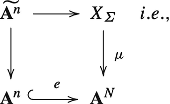
• 1. Given a divisorial valuation v centered at $0 \in {\mathbf {A}}^n,$ determine whether there exist an embedding $e: {\mathbf {A}}^n\hookrightarrow {\mathbf {A}}^N,$ (where N depends on v) and a toric proper birational morphism $\mu : X_{\varSigma }\longrightarrow {\mathbf {A}}^N$ such that:

  

  • $X_{\varSigma }$ is a smooth toric variety (i.e.,$\varSigma$ is a fan which is obtained by a regular subdivision of the positive quadrant ${\mathbf {R}}_+^N,$ this quadrant is the cone defining ${\mathbf {A}}^N$ as a toric variety),

  • the strict transform $\widetilde {{\mathbf {A}}^n}$ of ${\mathbf {A}}^n$ by $\mu$ is smooth,

  • there exists a toric divisor $E'\subset X_{\varSigma }$ which intersects $\widetilde {{\mathbf {A}}^n}$ transversally along a divisor $E,$

  • the valuation defined by the divisor E is $v.$

  Note that a toric divisor $E'$ centered at the origin 0 of ${\mathbf {A}}^N=\mathrm {Spec}\mathbf {K}[x_1,\ldots ,x_N]$ corresponds to a divisorial valuation $v'$ which is monomial, i.e., there exists a vector $\alpha \in {\mathbf {N}}^N$ such that $v'=v_\alpha$ where

  $$\displaystyle \begin{aligned} v_\alpha: \mathbf{K}[x_1,\ldots,x_N]\longrightarrow \mathbf{N}\end{aligned}$$

  is defined by: for $h\in \mathbf {K}[x_1,\ldots ,x_N],$

  $$\displaystyle \begin{aligned} {} h=\sum_{m=(m_1,\ldots,m_N)}a_mx_1^{m_1}\cdots x_N^{m_N},\ \ \ \ \ \ v_\alpha(h)=\mathrm{min}_{\{m\mid a_m\neq 0\}}<\alpha,m>; \end{aligned} $$

  (4.6)

  where $<\alpha ,m>$ is the usual scalar product on ${\mathbf {R}}^N.$

  Then one can formulate the conditions above by saying that there exists an embedding ${\mathbf {A}}^n\hookrightarrow {\mathbf {A}}^N$ such that v is the trace of a monomial valuation defined on ${\mathbf {A}}^N.$

• 2. Determine a finite number of significant divisorial valuations $v_1,\ldots ,v_r$ on ${\mathbf {A}}^n$ from the geometry of the jet schemes and the arc space of X (this step is to compare with the Nash problem that we mentioned above: very roughly speaking, as the Nash problem search for divisorial valuations that will “appear” on every resolution of singularities, here we are searching for divisorial valuations whose torifications in the sense of question (1) is essential to obtain a global torification), then embed as above ${\mathbf {A}}^n$ in a larger affine space ${\mathbf {A}}^N$ in such a way that all the valuations $v_1,\ldots ,v_r$ can be seen as the traces of monomial valuations on ${\mathbf {A}}^N.$

If $v_1,\ldots ,v_r,$ are well chosen, this should guarantee that the embedding $X \subset {\mathbf {A}}^N$ is torific. Let us discuss this last sentence which probably for now looks a bit prophetic. Let $v=v_{\alpha }$ be the monomial valuation defined on ${\mathbf {A}}^n=\mathrm {Spec} \mathbf {K}[x_1,\ldots ,x_n]$ by a vector $\alpha =(\alpha _1,\ldots ,\alpha _n),$ where $\alpha _i \in {\mathbb N},i=1,\ldots ,n.$ Let $I\subset \mathbf {K}[x_1,\ldots ,x_n]$ be an ideal such that the origin 0 belongs to the variety $V(I)\subset {\mathbf {A}}^n=\mathrm {Spec} \mathbf {K}[x_1,\ldots ,x_n]$ defined by it. We will say that I or $V(I)$ is non-degenerate with respect to v at 0 if the singular locus of the variety defined by the initial ideal $in_{v}(I)$ of I does not intersect the torus $({\mathbf {K}}^*)^n.$ Note that in this context, the initial ideal of I relative to v is defined by

$$\displaystyle \begin{aligned} in_{v}(I)=\{in_{v}(f),f\in I \},\end{aligned}$$

where for $f=\sum a_{i_1,\ldots ,i_n}x_1^{i_1}\cdots x_n^{i_n}\in \mathbf {K}[x_1,\ldots ,x_n],$

$$\displaystyle \begin{aligned} in_{v}(f)=\sum_{a_{i_1,\ldots,i_n}\neq 0, i_1\alpha_1+\cdots+i_n\alpha_n=v(f)} a_{i_1,\ldots,i_n}x_1^{i_1}\cdots x_n^{i_n}.\end{aligned}$$

It follows from [10, 11, 112, 130] (see also [134] for the hypersurface case) that if for every $\alpha =(\alpha _1,\ldots ,\alpha _n),\alpha _i \in \mathbf {N},i=1,\ldots ,n,$I is Newton non-degenerate with respect to $v_{\alpha }$ at $0,$ then we can construct a proper toric birational morphism $Z\longrightarrow {\mathbf {A}}^n$ that resolves the singularities of $V(I)$ in a neighborhood of $0.$ Notice that I can be degenerate with respect to a valuation defined by a vector ${\alpha }$ if there exists an irreducible family of jets (having a large contact with $V(I)$) or arcs on $V(I)$ such that for a generic $\gamma =(\gamma _1(t),\ldots ,\gamma _n(t))$ in this family, its order vector$(ord_t \gamma _1(t),\ldots ,ord_t\gamma _n(t))=\alpha :$ indeed, by a Newton-Puiseux type theorem (or the fundamental theorem of tropical geometry [94]), if this is not satisfied, i.e., if there is no arc, $in_{v_{\alpha }}(f)$ will contain monomials, hence by definition I will be non-degenerate with respect to $v_{\alpha }.$ This suggests that arcs detect Newton degeneration, and wherever there is a Newton degeneration, there is a degenerate arc passing there in the following sense: An arc defines a germ of a curve; we call an arc degenerate whenever the associated curve germ cannot be resolved with one toric morphism (this can also be detected from the properties of the arc, for instance using the notion of Nash multiplicity [83]). There are degenerate arcs that can be traced on a smooth variety: think of a (relatively) nasty plane curve like the germ of curve which is defined by $(\{(y^2-x^3)^2-4x^5y-x^7=0\},0) \subset ({\mathbf {A}}^2,0)=\{z=y\}\subset ({\mathbf {A}}^3,0);$ it is associated with the arc $(t^4,t^6+t^7,t^6+t^7)$ which is traced on ${\mathbf {A}}^2.$ The arc is degenerate but ${\mathbf {A}}^2\subset {\mathbf {A}}^3$ is Newton non-degenerate. The moral of this part of the story is first that Newton degeneration is detected by degenerate arcs, and second that not all degenerate arcs cause Newton degeneration. Moreover, the notion of degeneration along an arc can be quantified by an invariant that one can call depth and which in the case of a plane curve is the number of Puiseux pairs minus one. Question (1) above takes care of this notion of depth and it allows by embedding in higher dimension the elimination of degeneration along a family of arcs (or jets) that defines a divisorial valuation. Question (2) concerns the determination of those families of arcs that cause Newton degeneration.

We will now give a presentation of results concerning these two questions, with some digressions in order to give applications, links between the two questions and expand a bit some problems that appear inside these questions and which are interesting for their own sakes.

Let us begin by discussing one aspect of question (1). While this question was exposed as a geometric problem, it is related to an “algebraic” problem which makes sense for any valuations: determining a generating sequence of a valuation. Let us for a moment stick to the case of a divisorial valuation centered at the origin $X={\mathbf {A}}^d=\mathrm {Spec}R,$ where $R=\mathbf {K}[x_1,\ldots ,x_n]$ is a polynomial ring over an algebraically closed field $\mathbf {K}.$ A valuation v is then given by a mapping $v:R\longrightarrow {\mathbb N}$ which is the order of vanishing along a divisor $E\subset Z$ which satisfies $\mu (E)$ is the origin of ${\mathbf {A}}^n,$$\mu$ being a birational map $\mu :Z\longrightarrow {\mathbf {A}}^n.$ Let us explain what is a generating sequence of $v.$

For $\alpha \in {\mathbb N}$, let

$$\displaystyle \begin{aligned} \mathcal{P}_{\alpha}=\{ h \in R\mid v(h)\geq \alpha \}.\end{aligned}$$

We define the $\mathbf {K}$-graded algebra

$$\displaystyle \begin{aligned} gr_{v}R=\bigoplus_{\alpha \in {\mathbb N}} \frac{\mathcal{P}_{\alpha}}{\mathcal{P}_{\alpha+1}}.\end{aligned}$$

We call $in_{v}$ the natural map

$$\displaystyle \begin{aligned} in_{v}: R\longrightarrow gr_{v}R,~~h\mapsto h ~~\mbox{mod}~~\mathcal{P}_{v(h)+1} .\end{aligned}$$

Definition 4.7.1 ([124])

A generating sequence of v is a set of elements of R such that their image by $in_{v}$ generates $gr_{v}R$ as a $\mathbf {K}$-algebra.

This notion (for any valuation) is central in an earlier version of Spivakovsky’s approach [124] to local uniformization and in the present approach of Teissier to the same problem [130], with the difference that Teissier restricts his analysis to minimal generating sequences for rational valuations. In general, it is very difficult to determine a generating sequence of a given valuation, apart in dimensions 1 and $2;$ an abstract approach follows from the valuative Cohen theorem [130]. A remarkable advance in this direction was done for (rational) valuations in [40], as discussed below. We will show below, at least on an example, the relation between this notion and question (1). We will discuss first our new approach from [100] for the study of generating sequences of divisorial valuations defined as above. For that, we will use the representation of a divisorial valuation as the order of vanishing along a family of arcs.

Let $X={\mathbf {A}}^n=\mathrm {Spec}~R,$ as above. We have a natural truncation morphism $X_{\infty }\longrightarrow X,$ that we denote by $\varPsi _0;$ for a n-tuple of series, this simply gives the n-tuple of constant terms of these series. For $p\in {\mathbb N}$ and $Y=V(I)\subset X$ a subscheme defined by an ideal $I\subset R$, we consider the contact locus $Cont^p(Y)$ (see Eq. (4.5)).

With a fat irreducible component $\mathbf {W}$ of $Cont^p(Y),$ which is included in the fibre $\varPsi _0^{-1}(0)$ above the origin, we associate a valuation $v_{\mathbf {W}}:R\longrightarrow {\mathbb N}$ as follows:

$$\displaystyle \begin{aligned} v_{\mathbf{W}}(h)=\mbox{min}_{\gamma \in \mathbf{W}}\{ord_t\gamma^*(h)\},\end{aligned}$$

for $h\in R.$ It follows from [50] (see also [45, 120], prop. 3.7 (vii)), that $v_{\mathbf {W}}$ is a divisorial valuation centered at the origin $0\in X,$ and that all divisorial valuations centered at $0\in X,$ can be obtained in this way (see Sect. 4.5) for varying ideals $I.$ We are interested in determining a generating sequence of a valuation of the form $v_{\mathbf {W}}$ with an irreducible component $\mathbf {W}$ of $Cont^p(Y).$ Recall from 4.2 or [17] the functorial definition of the arc space $X_\infty :$ for any algebraic variety $X,$ the arc space $X_\infty$ represents the functor that to a $\mathbf {K}$-algebra A associates the set of $A-$valued arcs

$$\displaystyle \begin{aligned} X(A[[t]]):=\mathrm{Hom}_{\mathbf{K}}(\mathrm{Spec} (A[[t]]),X).\end{aligned}$$

Hence, for a $\mathbf {K}$-algebra A we have a bijection

$$\displaystyle \begin{aligned} \mathrm{Hom}_{\mathbf{K}}(\mathrm{Spec} (A),X_\infty)\simeq \mathrm{Hom}_{\mathbf{K}}(\mathrm{Spec} (A[[t]]),X).\end{aligned}$$

In particular, in our case $X={\mathbf {A}}^n=\mathrm {Spec}R,$ we have $X_\infty =\mathrm {Spec}(R_\infty ),$ and to the identity in $\mathrm {Hom}_{\mathbf {K}}(\mathrm {Spec} (R_\infty ),X_\infty )$ corresponds the universal family $\varLambda :R\longrightarrow R_\infty [[t]].$

Let us consider the case $n=2,R=\mathbf {K}[x_0,x_1].$ We have

$$\displaystyle \begin{aligned} R_\infty=\mathbf{K}[x_i^{(j)};i=0,1;j\geq 0],\end{aligned}$$

and $\varLambda$ is given by

$$\displaystyle \begin{aligned} \varLambda(x_i)=x_i^{(0)}+x_i^{(1)}t+x_i^{(2)}t^2+\cdots,\ \ \ i=0,1.\end{aligned}$$

The procedure that we give can be thought as an elimination algorithm with respect to $\varLambda$ in the sense that from the equations (that we can see in $R_\infty$) of the irreducible component of $Cont^p(Y)$ defining our valuation we will obtain elements in R that constitute the generating sequence. Let us show this on an example: Assume that the characteristic is not equal to $2.$ Let us consider the divisorial valuation associated with one irreducible component of $Cont^{27}(Y),$ where Y  is the curve defined by the equation $(x_1^2-x_0^3)^2-x_0^5x_1=0.$ The contact locus $Cont^{27}(Y)$ has two irreducible components which are sent to the origin 0 by the truncation morphism $\pi _{27},$ the interesting one (the other one gives a monomial valuation), that we call $\mathbf {W}$ is defined in ${\mathbf {A}}^2_\infty$ by the ideal generated by

$$\displaystyle \begin{aligned} x_0^{(0)},\ldots, x_0^{(3)},x_1^{(0)},\ldots,x_1^{(5)}, {x_1^{(6)}}^2-{x_0^{(4)}}^3,\end{aligned}$$

$$\displaystyle \begin{aligned} (2x_1^{(6)}x_1^{(7)}-3{x_0^{(4)}}^2x_0^{(5)})^2-{x_0^{(4)}}^5x_1^{(6)}\end{aligned}$$

and two inequalities, the most important one of them is $x_0^{(4)}\neq 0.$ Noticing that the first equation which is not that of a coordinate hyperplane being not linear, this gives us the first three elements of a generating sequence

$$\displaystyle \begin{aligned} x_0,x_1,x_2=x_1^2-x_0^3.\end{aligned}$$

The last element was obtained by what we called an elimination process which corresponds here to dropping the indices in the parentheses from ${x_1^{(6)}}^2-{x_0^{(4)}}^3.$ Note that modulo $x_0^{(0)}=\cdots = x_0^{(3)}=x_1^{(0)}=\ldots =x_1^{(5)}=0,$$\varLambda (x_2)= ({x_1^{(6)}}^2-{x_0^{(4)}}^3)t^{12}+t^{13}\phi , \ \text{ with }\ \phi \in R_\infty [[t]].$ The remaining equation, modulo the other equations, can then be rewritten

$$\displaystyle \begin{aligned} (2x_1^{(6)}x_1^{(7)}-3{x_0^{(4)}}^2x_0^{(5)})^2-{x_0^{(4)}}^5 x_1^{(6)}={x_2^{(13)}}^2-{x_0^{(4)}}^5x_1^{(6)}.\end{aligned}$$

Again, the elimination process with respect to $\varLambda$ corresponds to dropping the indices in the parentheses. The 4th and last element of the generating sequence of $v_{\mathbf {W}}$ which is then:

$$\displaystyle \begin{aligned} x_3=x_2^2-x_0^5x_1.\end{aligned}$$

The valuation $v_{\mathbf {W}}$ is completely determined by its generating sequence $x_0,x_1,x_2,x_3$ and the values $v_{\mathbf {W}}(x_0)=4,v_{\mathbf {W}}(x_1)=6,v_{\mathbf {W}}(x_2)=13, v_{\mathbf {W}}(x_3)=27.$ By construction, for $i=2,3$ we have polynomials $f_i$ such that

$$\displaystyle \begin{aligned} x_{i}=f_i(x_0,\ldots,x_{i-1}).\end{aligned}$$

The functions $f_i$’s provide an embedding ${\mathbf {A}}^2\hookrightarrow {\mathbf {A}}^{4},$ which is the geometric counterpart of the following morphism

$$\displaystyle \begin{aligned} \mathbf{K}[x_0,x_1,x_2,x_{3}]\longrightarrow \frac{\mathbf{K}[x_0,x_1,x_2,x_{3}]}{(x_2-f_2(x_0,x_1),x_3-f_3(x_0,x_1,x_2))}\simeq \mathbf{K}[x_0,x_1].\end{aligned}$$

This embedding solves question (1) for the valuation $v_{\mathbf {W}}$ and realizes this latter as the trace of the monomial valuation centered at $({\mathbf {A}}^4,0)$ and associated with the vector $\alpha =(4,6,13,27).$ Here we only gave the feeling of this, but the reason why the second and the third points of question (1) are satisfied follows from the fact that if $\nu =\nu _\alpha$ then the initial ideal of $(x_2-f_2(x_0,x_1),x_3-f_3(x_0,x_1,x_2))$ with respect to $\nu$ is given by

$$\displaystyle \begin{aligned} (x_1^2-x_0^3,x_2^2-x_0^5x_1),\end{aligned}$$

which is a toric (prime) ideal and its singular locus is a point. More generally we have

Theorem 4.7.2 ([100])

For $n=2,$ there is a constructive solution of question (1).

It is important to mention here that determining a generating sequence is not necessary to solve question (1) for a given valuation.

We can give now an example of our geometric approach to the resolution of singularities. Let $Y\subset {\mathbf {A}}^2$ be again the curve defined by $(x_1^2-x_0^3)^2-x_0^5x_1=0.$ The interesting divisorial valuation is the one associated with the irreducible component of $Y_{25}$ (or equivalently of $Cont^{26}(Y))$ which is defined by the ideal

$$\displaystyle \begin{aligned} \left(x_0^{(0)},\ldots, x_0^{(3)},x_1^{(0)},\ldots,x_1^{(5)}, {x_1^{(6)}}^2-{x_0^{(4)}}^3\right).\end{aligned}$$

We do not explain here in detail why we choose this divisor but we can say that this is the most natural choice which arises from the geometry of the jet schemes, which will be discussed below. But we can say that the space of arcs (on Y ) centered at the singular point of Y  has one irreducible component whose geometry is reflected by the geometry of this irreducible component of $Y_{25}.$ Applying the procedure that we explained above, we find an embedding ${\mathbf {A}}^2\hookrightarrow {\mathbf {A}}^{3},$ which is the geometric counterpart of the following morphism

$$\displaystyle \begin{aligned} \mathbf{K}[x_0,x_1,x_2]\longrightarrow \frac{\mathbf{K}[x_0,x_1,x_2]}{(x_2-({x_1}^2-{x_0}^3))}\simeq \mathbf{K}[x_0,x_1].\end{aligned}$$

Our curve Y  seen in ${\mathbf {A}}^3$ is then defined by the ideal

$$\displaystyle \begin{aligned} I=(x_2-({x_1}^2-{x_0}^3),x_2^2-x_0^5x_1).\end{aligned}$$

Its (local) tropical variety (with respect to the embedding in ${\mathbf {A}}^3)$ is the half line along the vector $(4,6,13)$ (see [116] for the notion of local tropical variety). The initial ideal of I with respect to the monomial valuation associated with the vector $(4,6,13)$ is given by the ideal

$$\displaystyle \begin{aligned} J=(x_1^2-x_0^3,x_2^2-x_0^5x_1).\end{aligned}$$

The singular locus of the variety defined by this latter ideal (which actually defines a monomial curve) is just a point so that this ideal is non-degenerate and can be resolved with one toric morphism. Hence, this embedding is torific; more generally, this gives another proof of torification for analytically irreducible plane curves [58]. Now applying our geometric approach to resolution of singularities to a reducible plane curve we were able with de Felipe and González-Pérez to prove in the following:

Theorem 4.7.3 ([41])

For a reducible plane curve singularity, the geometric approach to resolution of singularities yields a torific embedding.

We can actually construct a torification for curves of any embedding dimension. What makes things more complicated in higher dimensions, is that the initial ideal which is the counter part of the initial ideal that we called J above, is not toric, but it still corresponds to a $T-$ variety (i.e.,) a variety which is equiped with an action of a torus of smaller dimension. Some work in this direction is in the ongoing project [19].

4.8 Deformations of Jet Schemes

In this section, we work over the field of complex number $\mathbf {C}.$ Equisingularity theories were introduced by Whitney, Zariski, Teissier, Lê and others [113, 128, 129, 133, 137] to compare singularities in a family with respect to algebraic, topological, geometric or differential invariants. The theory of jet schemes allow to consider two new equisingularity conditions; let $\mathfrak {X}$ be a (flat) family of singularities defined over a base variety $B.$ One may wonder when $\mathfrak {X}\longrightarrow B$ induces a (flat) deformation $\mathfrak {X}_m\longrightarrow B$ (or a deformation $(\mathfrak {X}_m)_{red}\longrightarrow B$ for every $m\in \mathbf {N}.$ In general, this is not the case; for instance for the embedded family $\mathfrak {X}\longrightarrow (\mathbf {C},0)$ which is defined by

$$\displaystyle \begin{aligned} \mathfrak{X}=\{y^2-ux^2-x^3=0\}\subset ({\mathbf{C}}^3,0),\end{aligned}$$

where u is the parameter of the deformation, $(\mathfrak {X}_m)_{red}\longrightarrow B$ is not flat; this follows for instance from the fact that dimension of $(\mathfrak {X}_u)_5$ (where $\mathfrak {X}_u$ is the fiber over u) depends on whether $u\neq 0$ or $u=0:$ it is 6 for $u\neq 0$ and 7 if $u=0.$ For plane irreducible curves, it follows from [97] that:

Theorem 4.8.1 ([97])

Let $\mathfrak {X}\longrightarrow B$ be a (flat) family of irreducible plane curve singularities over a smooth variety $B.$ The induced family $(\mathfrak {X}_m)_{red}\longrightarrow B$ is flat for every $m\in \mathbf {N}$ if and only if the fibers of $\mathfrak {X}$ have the same semigroup.

In the theorem, the notion of semigroup is attached to a plane curve and is defined via the local intersection multiplicity of the curve at the origin; this latter defines a valuation whose semigroup is by definition the semigroup of the curve [138].

Note that, all the known equisingularity theories for families of plane curves are equivalent: such a family is equisingular if every fiber has the same semigroup (or equivalently the same Puiseux pairs). It follows from [105] that this theorem is no longer true if we allow fibers which are not necessarily plane curves.

Leyton-Alvarez [87, 88] gave a sufficient condition for an embedded one parameter family of hypersurfaces $\mathfrak {X}\subset ({\mathbf {C}}^{d+1},0)\times (\mathbf {C},0)$ to induce a flat deformation:

Theorem 4.8.2 (Leyton-Alvarez)

Let $\mathfrak {X}\subset ({\mathbf {C}}^{d+1},0)\times (\mathbf {C},0)$ be a flat family of hypersurfaces. If the family $\mathfrak {X} \subset ({\mathbf {C}}^{d+1},0)\times (\mathbf {C},0)$ admits a simultaneous embedded resolution then it induces a flat family $(\mathfrak {X}_m)_{red}\longrightarrow (\mathbf {C},0)$ for every $m\in \mathbf {N}.$

We refer to [89] for a precise definition of a simultaneous embedded resolution. The following theorem of Leyton-Alvarez, Mourtada and Spivakovsky is proved in [89].

Theorem 4.8.3 ([89])

Let $\mathfrak {X}\subset ({\mathbf {C}}^{d+1},0)\times (\mathbf {C},0)$ be a flat Newton non-degenerate family of isolated hypersurface singularities. If $\mathfrak {X}$ is $\mu$ -constant then it induces a flat family $(\mathfrak {X}_m)_{red}\longrightarrow (\mathbf {C},0)$ for every $m\in \mathbf {N}.$

Let us say that a family $\mathfrak {X}\longrightarrow B$ is jet schemes equisingular if it induces a flat family $(\mathfrak {X}_m)_{red}\longrightarrow B$ for every $m\in \mathbf {N}.$ It is a very interesting line of research to compare this notion of equisingularity with the other existing notions.

4.9 Arc Spaces and Integer Partitions

This line of research again finds its origin in the study of singularities as we will show later but is now making its way into the world of combinatorics and classical number theory, so let us begin there. The following identity

$$\displaystyle \begin{aligned} {} 1+\frac{e^{-2\pi}}{1+\frac{e^{-4\pi}}{1+\frac{e^{-6\pi}}{\vdots}}}= \left(\sqrt{\frac{5+\sqrt{5}}{2}}-\frac{1+\sqrt{5}}{2}\right)e^{\frac{2\pi}{5}} \end{aligned} $$

(4.7)

was imagined by Ramanujan and sent to Hardy who says in the article “The Indian Mathematician Ramanujan” (Amer. Math. Monthly 44 (1937), p. 144), see also [8]:

[These formulas] defeated me completely. I had never seen anything in the least like them before. A single look at them is enough to show that they could only be written down by a mathematician of the highest class. They must be true because, if they were not true, no one would have had the imagination to invent them.

Some years later, Ramanujan gave a proof of this formula by considering the following $q-$difference equation

$$\displaystyle \begin{aligned} {} F(x)=F(xq)+xqF(xq^2), \end{aligned} $$

(4.8)

where $q\in {\mathbf {C}}^*,$ and $F(x)=\sum a_n(q)x^n$ is an analytic function satisfying $F(0)=1.$

If we define $c(x,q):=\frac {F(x)}{F(xq)},$ notice that we have

$$\displaystyle \begin{aligned} c(x,q)=1+\frac{xq}{c(xq,q)}=1+\frac{xq}{1+\frac{xq^2}{c(xq^2,q)}}.\end{aligned}$$

Iterating this last identity we obtain that the left member of the identity (4.7) is equal to $c(1,e^{-2\pi }).$ Now if we plug $F(x)=\sum a_n(q)x^n$ in the Eq. (4.8), by comparing the coefficients of $x^n$ we get

$$\displaystyle \begin{aligned} a_n(q)=\frac{q^{n^2}}{(q)_n}=\frac{q^{n^2}}{(1-q)(1-q^2)\cdots (1-q^n)}.\end{aligned}$$

The miracle arrives in the following identity

(4.9)

The left hand side in the identity (4.9) is $F(1).$ There is another miracle which is that $F(q)$ is also an infinite product and hence $c(1,q)$ is. And we may then deduce Ramanujan’s continued fraction (4.7) by an appeal to the theory of elliptic theta functions.

The “miracles” above are called the Rogers-Ramanujan identities; they have appeared “in many different situations”: in statistical mechanics, number theory, representation theory …and we came to them first with Clemens Bruschek and Jan Schepers via Arc spaces. Before telling the story, let us state another version of the first Rogers-Ramanujan identity (4.9).

Definition 4.9.1

A partition of a positive integer n is a decreasing sequence $\varLambda =(\lambda _1\geq \lambda _2\geq \cdots \geq \lambda _r)$ such that $\lambda _1+\cdots +\lambda _r=n.$ The $\lambda _i$’s are called the parts of this partition and r is its size.

The identity (4.9) can be stated as follows:

Theorem 4.9.2 (Rogers, Ramanujan)

The number of partitions of n with neither consecutive parts nor equal parts (of first type) is equal to the number of partitions of n whose parts are congruent to 1 or 4 modulo 5 (of second type).

The generating series of the cardinality of the partitions of the first type is the left hand member in the identity (4.9) and the generating series of the cardinals of the partitions of the second type is the right hand member in (4.9), i.e., the infinite product. Now we go back to algebraic geometry and to arc spaces. Let $(X,0)$ be a singularity defined over a field $\mathbf {K}$ which is assumed for simplicity to be of characteristic 0 for (0 being a closed point that after a change of coordinates may be chosen to be the origin of an affine space containing $(X,0)$). Let $X_\infty ^0=\mbox{Spec} A_\infty ^0$ be the space of arcs centered at the point $0.$ It has a natural cone structure which induces a grading on $A_\infty ^0$ (i.e.,$A_{\infty }^0=\oplus _{h\in \mathbf {N}}A_{\infty ,h}^0)$ and one can consider its Hilbert-Poincaré series that we call the Arc-Hilbert-Poincaré series of the singularity:

$$\displaystyle \begin{aligned} \mbox{AHP}_{X,0}=\sum_{h\in \mathbf{N}} \dim_{\mathbf{K}} A_{\infty,h}^0~q^h.\end{aligned}$$

It is not difficult to see that this is an invariant of singularities (it detects regularity) and it contains different ingredients which motivate its study from the viewpoint of singularity theory: First, if $X\subset {\mathbf {A}}^e$ and considering the jet schemes $X_m\subset {\mathbf {A}}^e_m={\mathbf {A}}^{e(m+1)}$ and $X^0_m\subset {({\mathbf {A}}^e)}_m^0={\mathbf {A}}^{em};$

• (i) one notices on examples that the defining ideal of $X^0_m$ in ${\mathbf {A}}^{em}$ is independent of some of the variables of the polynomial ring which is the ring of global sections of ${\mathbf {A}}^{em}$ and that the number of variables needed to define this ideal (modulo a linear change of variables) depends on how singular X is at $0.$ The more X is singular, the less variables we need for a given $m;$ such an invariant was actually defined by Hironaka as a resolution invariant, see for instance [16] but this is another story.

• (ii) The data of an $m-$jet determines its coordinates in ${\mathbf {A}}^{em}$ and as mentioned in the item (1), there are no constraints on some of these coordinates; but there are constraints on these “free coordinates” for the jet to be liftable to an arc and these constraints come from the equations defining $X_l$ for $l\geq m;$ the smallest l such that the equations defining $X_l$ catch all the constraints on all the $m-$jets for them to be liftable is related to the Artin-Greenberg function which is another invariant of singularities [65, 122]: roughly speaking, Greenberg’s theorem states that if a tuple $\gamma (t)$ of power series in $\mathbf {K}[[t]]$ is very close in the t-adic topology to being an arc on X (which means that $\gamma$ coincides with an $r-$jet on X for some large r) then there is an actual arc $\gamma '$ on X which is close to $\gamma$ in the sense that $\gamma$ coincides to $t-$adic order m with the $m-$jet of $\gamma '$; the Artin-Greenberg function $\beta (m)$ measures how close you need to be to an arc on X to have the same m-jet as an arc on X; again, roughly speaking, the larger the function is, the nastier the singularity $(X,0)$ is.

The Arc Hilbert Poincaré series is related in spirit to these two types of invariants: Heuristically, the more we have free variables at the level $m,$ the larger will be the dimension of the homogeneous components of $A_{\infty }^0$ of weight less than or equal to m will be (note that the homogeneous components of weight less than or equal to m are the same as those of the ring of global sections of $X_m^0$) but also the larger is the Artin-Greenberg function. But this invariant is very difficult to compute, because of the complicated homological properties of $A^0_{\infty }$ in general, even though sometimes for mild singularities this is possible, [26]:

Theorem 4.9.3 ([26])

Let X be a normal hypersurface in ${\mathbf {A}}^n$ with a canonical singularity of multiplicity $n - 1$ at the origin. Then

$$\displaystyle \begin{aligned} \mathrm{AHP}_{X,0}(q)=\left(\prod_{i=1}^{n-2}\frac{1}{1-q^i}\right)^{n} \left(\prod_{i\geq n-1}\frac{1}{1-q^i}\right)^{n-1}.\end{aligned}$$

This generalizes a theorem that was obtained in [99] for rational double point surface singularities. Some research is still ongoing to reveal the secrets of this invariant of singularities but let us go back now to partitions and to a beautiful link with the Arc-Hilbert-Poincaré series [25]:

Theorem 4.9.4 ([25])

$$\displaystyle \begin{aligned} \mathit{\mbox{For}}~~~X=\mathit{\mbox{Spec}}\frac{\mathbf{K}[x]}{(x^2)},~~~ \mathrm{AHP}_{X,0}(q)=\prod_{i\equiv~1,4~~(\mathit{\mbox{mod}}~5)}\frac{1}{1-q^i}.\end{aligned}$$

Notice that the power series in the theorem is the right hand side of the first Rogers Ramanujan identity. The proof uses the differential structure of $A_{\infty }^0$ which for $X=\mbox{Spec}\frac {\mathbf {K}[x]}{(x^2)}$ is given by

$$\displaystyle \begin{aligned} A_{\infty}^0=\frac{\mathbf{K}[x_i,i \in {\mathbf{N}}_{>0}]}{[x_1^2]},\end{aligned}$$

where $[x_1^2]$ is the differential ideal generated by $x_1^2$ and its iterated derivatives with respect to the derivation D which is determined by $D(x_i)=x_{i+1}.$ So

$$\displaystyle \begin{aligned} {} [x_1^2]= (x_1^2,2x_1x_2,2x_1x_3+2x_2^2,\ldots) \end{aligned} $$

(4.10)

The grading of $A_{\infty }^0$ is induced from the weights given to the variables, $x_i$ being of weight $i.$ We order the monomials using an “adapted” monomial ordering, the weighted reverse lexicographical ordering; Now, it is well known that the Hilbert Poincaré series of the quotient ring by an ideal I is equal to the Hilbert Poincaré series of the quotient ring by the leading ideal (relative to a monomial ordering which respects the weight) of $I.$ This latter is generated by the leading monomials of the elements of a Groebner basis of $I.$ In general, it is very complicated to find a Groebner basis theoretically, even when we consider, let us say, the ideal generated by the first 5 generators of $I:=[x_1^2],$ we should add many polynomials to obtain a Groebner basis [12]; the miracle is that the generators in (4.10) give a Groebner basis with respect to the weighted reverse lexicographical ordering. The proof shows actually that any S-polynomial (this is a notion used in Buchberger algorithm for computing a Groebner basis) is not relevant and it comes out, after determining its weight $w,$ from the $(w-4)-$th derivative (by D) of the equation

$$\displaystyle \begin{aligned} 2x_2(x_1^2)-x_1(2x_1x_2)=0.\end{aligned}$$

We deduce that

$$\displaystyle \begin{aligned} \mbox{AHP}_{X,0}(q)=\mbox{HP}(\frac{\mathbf{K}[x_i,i \in \mathbf{N}]}{\left(x_i^2,x_ix_{i+1}; i\in {\mathbb N}_{>0}\right)}),\end{aligned}$$

where HP stands for the Hilbert-Poincaré series and where the ideal

$$\displaystyle \begin{aligned} (x_i^2,x_ix_{i+1};i\in {\mathbb N}_{>0})\end{aligned}$$

is the leading ideal of $[x_1^2].$ Now after a short reasoning, one sees that $\mbox{HP}(\frac {\mathbf {K}[x_i,i \in {\mathbb N}]}{(x_i^2,x_ix_{i+1}; i\in {\mathbb N}_{>0})})$ is exactly the generating series of the number of partitions of n with neither consecutive nor equal parts. Using the first Rogers-Ramanujan identity we get the formula in the theorem.

Moreover, with very simple commutative algebra applied to

$$\displaystyle \begin{aligned} \mbox{HP}(\frac{\mathbf{K}[x_i,i \in \mathbf{N}]}{(x_i^2,x_ix_{i+1}; i\in {\mathbb N}_{>0})})\end{aligned}$$

we find that there is a sequence of power series in the variable q which converges in the $q-$adic topology to both sides of the Rogers-Ramanujan identities giving a commutative algebra approach to these identities; this sequence was stated in an empirical way in [9].

This theorem was greatly generalized in [26]:

Theorem 4.9.5 ([26])

For $X=\mathit{\mbox{Spec}}\frac {\mathbf {K}[x]}{(x^n)},$

$$\displaystyle \begin{aligned} \mathit{\mbox{AHP}}_{X,0}(q)=\prod_{i\not\equiv~~0,n,n+1~~\mathit{\mbox{mod}}(2n+1)}\frac{1}{1-q^i}.\end{aligned}$$

The proof uses similar ideas but the differential calculus is much more involved. This latter theorem is related to Gordon’s identities which are partition identities generalizing the Rogers-Ramanujan identities. A commutative algebra proof of Gordon’s identities was found in the PhD thesis of Pooneh Afsharijoo [4].

Now recall that in the proof of Theorem 4.9.3, we considered the Groebner basis of the ideal $[x_1^2]$ with respect to the weighted reverse lexicographical ordering; the heuristic reason of the choice of this ordering is that this allows to see first (i.e., as leading monomials) the monomials which concern the larger neighborhoods from the point of view of Taylor series: for instance for the polynomial $x_2^2+x_1x_3,$ the leading term with respect to the reverse lexicographical ordering is $x_2^2$ which concerns an approximation of order 2 while $x_1x_3$ concerns an approximation of order $3.$ But as mentioned before, the Hilbert series of the quotient by the ideal $[x_1^2]$ is equal to the Hilbert series of the quotient by its leading monomial ideal with respect to any monomial ordering respecting the weight. With Pooneh Afsharijoo, we considered the weighted lexicographical ordering and we knew that if we catch the leading monomial ideal of $[x_1^2]$ with respect to this ordering, its Hilbert series will be equal to the generating series of the number of partitions appearing in the Rogers-Ramanujan identities, but potentially it counts partitions with different properties. The problem is that while the Groebner basis of $[x_1^2]$ with respect to the weighted reverse lexicographical ordering is differentially finite (i.e., it is obtained from a finite number of polynomials -here only one polynomial- and all their derivatives), we were able to prove that with respect to the weighted lexicographical ordering, there is no Groebner basis of $[x_1^2]$ which is differentially finite [7]; A Groebner basis is then very difficult to determine; but using Groebner basis theory computations, we were able to conjecture what is the leading monomial ideal of $[x_1^2];$ this remains a conjecture but we were able to prove that the Hilbert series of the quotient by this monomial ideal is equal to the series appearing in the Rogers-Ramanujan identities. By taking a variation of the ideal $[x_1^2],$ we have been led to the following partition identities [7] where for a partition $\lambda$ we denote by $s(\lambda )$ its smallest part.

Theorem 4.9.6 ([7])

Let $n\geq k$ be positive integers. The number of partitions $\lambda$ of n whose parts are larger or equal to k and whose size is less than or equal to $s(\lambda ) -(k-1)$ is equal to the number of partitions of n with parts larger or equal to k and without neither consecutive nor equal parts.

For $k=1,$ this gives another member of Rogers-Ramanujan identities: Let $n\geq 1$ be a positive integer. The number of partitions of n with size less than or equal to the smallest part is equal to the number of partitions of n without consecutive nor equal parts.

It is playful to see this last identity on the partitions of 4 but let us first call the partitions of n with size less than or equal to the smallest part, partitions of third type; partitions of first and second type were defined in Theorem 4.9.2. The partitions of 4 are

$$\displaystyle \begin{aligned} \begin{array}{rcl} 4 & = &\displaystyle 4 \\ & = &\displaystyle 3+1 \\ & = &\displaystyle 2+2 \\ & = &\displaystyle 2+1+1 \\ & = &\displaystyle 1+1+1+1 \end{array} \end{aligned} $$

The partitions of 4 which are of the first type are the first and the second partitions.

The partitions of 4 which are of the second type are the first and the fifth partitions.

The partitions of 4 which are of the third type are the first and the third partitions. And as the theorem predicts, the number of these partitions, two, is the same for the three types.

Using an idea similar to the one used to guess Theorem 4.9.6, Pooneh Afsharijoo has conjectured in her thesis new identities which add new members to Gordon’s identities [4, 6]; she proved this conjecture in a particular case and very recently with Pooneh Afsharijoo, Jehanne Dousse and Frédéric Jouhet, we proved these very exciting identities in general, this is the content of [5] (see also [3]).

These theorems are small steps (walking steps towards another planet) in studying what we would like to call Ramanujan Hilbert scheme, which parametrizes the schemes with a cone structure and whose Hilbert series is equal to $F(1).$

There are various generalizations of these theorems or these line of thoughts. I can mention for instance [96] or a theorem on partitions of two colours in [7].

4.10 Completions of Localizations of the Algebra of Arcs

We assume for simplicity that we are working over an algebraically closed field $\mathbf {K}$ of characteristic zero. Most of the invariants that we have considered in the previous section (apart form Sect. 4.9) made use of the reduced structure of the jet schemes or the space of arcs. This latter, being often of infinite dimension, its study requires commutative algebra in infinite dimension, which till now seems to be a difficult issue. Let X be a $\mathbf {K}$-algebraic variety; the local algebras of the arc space $X_\infty$ were studied for two types of points or arcs (for different reasons or motivations):

• The study of the local algebra of $X_\infty$ at a $\mathbf {K}$-rational arc $\gamma$ was motivated by some problems related to the Langlands program [24]. The first interesting theorem in this direction is the Drinfeld-Grinberg-Kazhdan theorem[20, 49, 63] which states that whenever $\gamma \not \in (Sing(X))_\infty ,$ there exists a finite dimensional $\mathbf {K}$-scheme $Y,$ a $\mathbf {K}$- point $y\in Y$ and an isomorphism

  $$\displaystyle \begin{aligned} \hat{\mathcal{O}}_{X_\infty,\gamma}\equiv \hat{\mathcal{O}}_{Y,y}\hat{\otimes}\mathbf{K}[[T_i,i\in \mathbf{N}]].~~~(\star)\end{aligned}$$

  The hat denotes the completion with respect to the maximal ideal. Bourqui and Sebag considered a minimal $\hat {\mathcal {O}}_{Y,y}$ in $(\star ),$ in the sense that $\hat {\mathcal {O}}_{Y,y}$ is not isomorphic to $B[[T]]$ (B being a local complete noetherian $\mathbf {K}$-algebra); this formal spectrum of $\hat {\mathcal {O}}_{Y,y}$ is then uniquely determined up to isomorphism and called the formal minimal model of X at $\gamma .$ For an irreducible plane curve singularity, the formal minimal model is independent of the choice the (primitive) arc $\gamma$ and thus defines an invariant of the singularity. For more about minimal formal models see [21,22,23, 30].

• The study of the local algebra of the arc space at a point associated with divisorial valuations (see the Sect. 4.3, see also [71, 119]); this was motivated by the Nash problem [119, 120]. It was proved by Reguera that for a divisorial valuation $\nu =\nu _E$ (E being the divisor) having a center on $X,$ denoting by $P_\nu$ the point in the arc space associated with $\nu ,$ the ring $\hat {\mathcal {O}}_{X_\infty ,P_\nu }$ is noetherian. Mourtada and Reguera found a formula relating the embedding dimension of $\hat {\mathcal {O}}_{X_\infty ,P_\nu }$ to the Mather discrepency$\hat {k}_E$ of E and found an upper bound of its dimension in terms of the Mather-Jacobian discrepancy [103].

Recently, there is a lot of interest on one hand (in the work of Bourqui, Sebag and others) in comparing the structure of $\hat {\mathcal {O}}_{X_\infty ,P_{\nu _E}}$ with the structure of the minimal formal model at a generic $\mathbf {K}$- arc in the family of arcs associated with E (see Sect. 4.3); and on the other hand in understanding the relation between the singularities of X and the structure of $\hat {\mathcal {O}}_{X_\infty ,P_\nu }$ in the continuity of [103] (see also [30]).

References

Shreeram Abhyankar. On the ramification of algebraic functions. Amer. J. Math., 77:575–592, 1955.
Dan Abramovich, Michael Temkin, and Jaroslaw Wlodarczyk. Functorial embedded resolution via weighted blowings up, 2019.
Afsharijoo Pooneh, Dousse Jehanne, Jouhe Frédéric, Mourtada Hussein New companions to gordon identities from commutative algebra. Sém. Lothar. Combin., Art 48(12):86B. 2022. 2021.
Pooneh Afsharijoo. Looking for a new version of Gordon’s identities, from algebraic geometry to combinatorics through partitions. PhD thesis, Université De Paris, 2019.
Afsharijoo Pooneh, Dousse Jehanne, Jouhe Frédéric, Mourtada Hussein New companions to the Andrews-Gordon identities motivated by commutative algera. Adv. Math, 417:Paper No. 108946, 40, 2023.
Pooneh Afsharijoo. Looking for a new version of Gordon’s identities. Ann. Comb., 25(3):543–571, 2021.
Pooneh Afsharijoo and Hussein Mourtada. Partition identities and application to infinite-dimensional Gröbner basis and vice versa. pages 145–161. World Sci. Publ., Hackensack, NJ, [2020] Ⓒ2020.
George E. Andrews. The theory of partitions. Encyclopedia of Mathematics and its Applications, Vol. 2. Addison-Wesley Publishing Co., Reading, Mass.-London-Amsterdam, 1976.
George E. Andrews and R. J. Baxter. A motivated proof of the Rogers-Ramanujan identities. Amer. Math. Monthly, 96(5):401–409, 1989.
Fuensanta Aroca, Mirna Gómez-Morales, and Hussein Mourtada. Groebner fans and embedded resolutions of ideals on toric varieties, 2022.
Fuensanta Aroca, Mirna Gómez-Morales, and Khurram Shabbir. Torical modification of Newton non-degenerate ideals. Rev. R. Acad. Cienc. Exactas Fís. Nat. Ser. A Mat. RACSAM, 107(1):221–239, 2013.
Yuzhe Bai, Eugene Gorsky, and Oscar Kivinen. Quadratic ideals and Rogers-Ramanujan recursions. Ramanujan J., 52(1):67–89, 2020.
Victor V. Batyrev. Non-Archimedean integrals and stringy Euler numbers of log-terminal pairs. J. Eur. Math. Soc. (JEMS), 1(1):5–33, 1999.
Angélica Benito and Orlando E. Villamayor U. Techniques for the study of singularities with applications to resolution of 2-dimensional schemes. Math. Ann., 353(3):1037–1068, 2012.
Angélica Benito and Orlando E. Villamayor U. Monoidal transforms and invariants of singularities in positive characteristic. Compos. Math., 149(8):1267–1311, 2013.
Jérémy Berthomieu, Pascal Hivert, and Hussein Mourtada. Computing Hironaka’s invariants: ridge and directrix. In Arithmetic, geometry, cryptography and coding theory 2009, volume 521 of Contemp. Math., pages 9–20. Amer. Math. Soc., Providence, RI, 2010.
Bhargav Bhatt. Algebraization and Tannaka duality. Camb. J. Math., 4(4):403–461, 2016.
Manuel Blickle. A short course on geometric motivic integration. In Motivic integration and its interactions with model theory and non-Archimedean geometry. Volume I, volume 383 of London Math. Soc. Lecture Note Ser., pages 189–243. Cambridge Univ. Press, Cambridge, 2011.
David Bourqui, Kevin Langlois, and Hussein Mourtada. The nash problem for torus actions of complexity one, 2022.
David Bourqui and Julien Sebag. The Drinfeld-Grinberg-Kazhdan theorem for formal schemes and singularity theory. Confluentes Math., 9(1):29–64, 2017.
David Bourqui and Julien Sebag. The minimal formal models of curve singularities. Internat. J. Math., 28(11):1750081, 23, 2017.
David Bourqui and Julien Sebag. Finite formal model of toric singularities. J. Math. Soc. Japan, 71(3):805–829, 2019.
David Bourqui and Julien Sebag. The local structure of arc schemes. pages 69–97. World Sci. Publ., Hackensack, NJ, [2020] Ⓒ2020.
A. Bouthier, B. C. Ngô, and Y. Sakellaridis. On the formal arc space of a reductive monoid. Amer. J. Math., 138(1):81–108, 2016.
Clemens Bruschek, Hussein Mourtada, and Jan Schepers. Arc spaces and Rogers-Ramanujan identities. In 23rd International Conference on Formal Power Series and Algebraic Combinatorics (FPSAC 2011), Discrete Math. Theor. Comput. Sci. Proc., AO, pages 211–220. Assoc. Discrete Math. Theor. Comput. Sci., Nancy, 2011.
Clemens Bruschek, Hussein Mourtada, and Jan Schepers. Arc spaces and the Rogers-Ramanujan identities. Ramanujan J., 30(1):9–38, 2013.
Nero Budur, Javier Fernández de Bobadilla, Quy Thuong Lê, and Hong Duc Nguyen. Cohomology of contact loci. J. Differential Geom., 120(3):389–409, 2022.
Jean-Baptiste Campesato. On a motivic invariant of the arc-analytic equivalence. Ann. Inst. Fourier (Grenoble), 67(1):143–196, 2017.
Antoine Chambert-Loir, Johannes Nicaise, and Julien Sebag. Motivic integration, volume 325 of Progress in Mathematics. Birkhäuser/Springer, New York, 2018.
Christopher Chiu, Tommaso de Fernex, and Roi Docampo. Embedding codimension of the space of arcs. Forum Math. Pi, 10:Paper No. e4, 37, 2022.
Raf Cluckers and François Loeser. Constructible exponential functions, motivic Fourier transform and transfer principle. Ann. of Math. (2), 171(2):1011–1065, 2010.
Helena Cobo and Hussein Mourtada. Jet schemes of quasi-ordinary surface singularities. Nagoya Math. J., 242:77–164, 2021.
Georges Comte and Goulwen Fichou. Grothedieck ring of semialgebraic formulas and motivic real Milnor fibers. Geom. Topol., 18(2):963–996, 2014.
Vincent Cossart and Olivier Piltant. Resolution of singularities of threefolds in positive characteristic. II. J. Algebra, 321(7):1836–1976, 2009.
Vincent Cossart and Olivier Piltant. Resolution of singularities of arithmetical threefolds. J. Algebra, 529:268–535, 2019.
Alastair Craw. An introduction to motivic integration. In Strings and geometry, volume 3 of Clay Math. Proc., pages 203–225. Amer. Math. Soc., Providence, RI, 2004.
Steven Dale Cutkosky. Resolution of singularities, volume 63 of Graduate Studies in Mathematics. American Mathematical Society, Providence, RI, 2004.
Steven Dale Cutkosky. Resolution of singularities for 3-folds in positive characteristic. Amer. J. Math., 131(1):59–127, 2009.
Steven Dale Cutkosky and Hussein Mourtada. Defect and local uniformization. Rev. R. Acad. Cienc. Exactas Fís. Nat. Ser. A Mat. RACSAM, 113(4):4211–4226, 2019.
Steven Dale Cutkosky, Hussein Mourtada, and Bernard Teissier. On the construction of valuations and generating sequences on hypersurface singularities. Algebr. Geom., 8(6):705–748, 2021.
Ana Belén de Felipe, Pedro D. González Pérez, and Hussein Mourtada. Resolving singularities of curves with one toric morphism, 2021.
Tommaso de Fernex. Three-dimensional counter-examples to the Nash problem. Compos. Math., 149(9):1519–1534, 2013.
Tommaso de Fernex. The space of arcs of an algebraic variety. In Algebraic geometry: Salt Lake City 2015, volume 97 of Proc. Sympos. Pure Math., pages 169–197. Amer. Math. Soc., Providence, RI, 2018.
Tommaso de Fernex and Roi Docampo. Terminal valuations and the Nash problem. Invent. Math., 203(1):303–331, 2016.
Tommaso de Fernex, Lawrence Ein, and Shihoko Ishii. Divisorial valuations via arcs. Publ. Res. Inst. Math. Sci., 44(2):425–448, 2008.
Jan Denef and François Loeser. Motivic Igusa zeta functions. J. Algebraic Geom., 7(3):505–537, 1998.
Jan Denef and François Loeser. Germs of arcs on singular algebraic varieties and motivic integration. Invent. Math., 135(1):201–232, 1999.
Roi Docampo and Antonio Nigro. The arc space of the Grassmannian. Adv. Math., 306:1269–1332, 2017.
Vladimir Drinfeld. The Grinberg-Kazhdan formal arc theorem and the Newton groupoids. pages 37–56. World Sci. Publ., Hackensack, NJ, [2020] Ⓒ2020.
Lawrence Ein, Robert Lazarsfeld, and Mircea Mustaţǎ. Contact loci in arc spaces. Compos. Math., 140(5):1229–1244, 2004.
Lawrence Ein and Mircea Mustaţă. Jet schemes and singularities. In Algebraic geometry—Seattle 2005. Part 2, volume 80 of Proc. Sympos. Pure Math., pages 505–546. Amer. Math. Soc., Providence, RI, 2009.
Lawrence Ein, Mircea Mustaţă, and Takehiko Yasuda. Jet schemes, log discrepancies and inversion of adjunction. Invent. Math., 153(3):519–535, 2003.
Lawrence Ein and Mircea Mustaţǎ. Inversion of adjunction for local complete intersection varieties. Amer. J. Math., 126(6):1355–1365, 2004.
J. Fernández de Bobadilla and M. Pe Pereira. The Nash problem from geometric and topological perspective. pages 173–195. World Sci. Publ., Hackensack, NJ, [2020] Ⓒ2020.
Javier Fernández de Bobadilla, María Pe Pereira, and Patrick Popescu-Pampu. On the generalized Nash problem for smooth germs and adjacencies of curve singularities. Adv. Math., 320:1269–1317, 2017.
Javier Fernández de Bobadilla and María Pe Pereira. The Nash problem for surfaces. Ann. of Math. (2), 176(3):2003–2029, 2012.
Yih-Nan Gau. Embedded topological classification of quasi-ordinary singularities. Mem. Amer. Math. Soc., 74(388):109–129, 1988. With an appendix by Joseph Lipman.
Rebecca Goldin and Bernard Teissier. Resolving singularities of plane analytic branches with one toric morphism. In Resolution of singularities (Obergurgl, 1997), volume 181 of Progr. Math., pages 315–340. Birkhäuser, Basel, 2000.
P. D. González Pérez. Bijectiveness of the Nash map for quasi-ordinary hypersurface singularities. Int. Math. Res. Not. IMRN, (19):Art. ID rnm076, 13, 2007.
Pedro D. González Pérez. Toric embedded resolutions of quasi-ordinary hypersurface singularities. Ann. Inst. Fourier (Grenoble), 53(6):1819–1881, 2003.
Pedro D. González Pérez and Manuel González Villa. Motivic Milnor fiber of a quasi-ordinary hypersurface. J. Reine Angew. Math., 687:159–205, 2014.
Pedro Daniel González Pérez. The semigroup of a quasi-ordinary hypersurface. J. Inst. Math. Jussieu, 2(3):383–399, 2003.
M. Grinberg and D. Kazhdan. Versal deformations of formal arcs. Geom. Funct. Anal., 10(3):543–555, 2000.
Herwig Hauser and Stefan Perlega. Cycles of singularities appearing in the resolution problem in positive characteristic. J. Algebraic Geom., 28(2):391–403, 2019.
M. Hickel. Calcul de la fonction d’Artin-Greenberg d’une branche plane. Pacific J. Math., 213(1):37–47, 2004.
Heisuke Hironaka. Resolution of singularities of an algebraic variety over a field of characteristic zero. I, II. Ann. of Math. (2)79 (1964), 109–203; ibid. (2), 79:205–326, 1964.
Ehud Hrushovski and David Kazhdan. Integration in valued fields. In Algebraic geometry and number theory, volume 253 of Progr. Math., pages 261–405. Birkhäuser Boston, Boston, MA, 2006.
Shihoko Ishii. Arc spaces and singularities. this volume.
Shihoko Ishii. The arc space of a toric variety. J. Algebra, 278(2):666–683, 2004.
Shihoko Ishii. Arcs, valuations and the Nash map. J. Reine Angew. Math., 588:71–92, 2005.
Shihoko Ishii. Maximal divisorial sets in arc spaces. In Algebraic geometry in East Asia—Hanoi 2005, volume 50 of Adv. Stud. Pure Math., pages 237–249. Math. Soc. Japan, Tokyo, 2008.
Shihoko Ishii. The minimal log discrepancies on a smooth surface in positive characteristic. Math. Z., 297(1–2):389–397, 2021.
Shihoko Ishii and János Kollár. The Nash problem on arc families of singularities. Duke Math. J., 120(3):601–620, 2003.
Shihoko Ishii and Ana J. Reguera. Singularities in arbitrary characteristic via jet schemes. In Hodge theory and\(L^2\)-analysis, volume 39 of Adv. Lect. Math. (ALM), pages 419–449. Int. Press, Somerville, MA, 2017.
Jennifer M. Johnson and János Kollár. Arc spaces of cA-type singularities. J. Singul., 7:238–252, 2013.
Heinrich W. E. Jung. Darstellung der Funktionen eines algebraischen Körpers zweier unabhängigen Veränderlichen \(x,y\) in der Umgebung einer Stelle \(x=a,\ y=b\). J. Reine Angew. Math., 133:289–314, 1908.
B. Karadeniz, H. Mourtada, C. Plénat, and M. Tosun. The embedded Nash problem of birational models of rational triple singularities. J. Singul., 22:337–372, 2020.
Hiraku Kawanoue and Kenji Matsuki. A new strategy for resolution of singularities in the monomial case in positive characteristic. Rev. Mat. Iberoam., 34(3):1229–1276, 2018.
K. Kiyek and M. Micus. Semigroup of a quasiordinary singularity. In Topics in algebra, Part 2 (Warsaw, 1988), volume 26 of Banach Center Publ., pages 149–156. PWN, Warsaw, 1990.
János Kollár. Lectures on resolution of singularities, volume 166 of Annals of Mathematics Studies. Princeton University Press, Princeton, NJ, 2007.
Kevin Langlois, Clélia Pech, and Michel Raibaut. Stringy invariants for horospherical varieties of complexity one. Algebr. Geom., 6(3):346–383, 2019.
Monique Lejeune-Jalabert. Arcs analytiques et resolution minimale des singularites des surfaces quasi homogènes. In Séminaire sur les Singularités des Surfaces, pages 303–336. Springer Berlin Heidelberg, 1980.
Monique Lejeune-Jalabert. Courbes tracées sur un germe d’hypersurface. Amer. J. Math., 112(4):525–568, 1990.
Monique Lejeune-Jalabert. The algebraic answer to the Nash problem for normal surfaces according to de Fernex and Docampo. pages 163–172. World Sci. Publ., Hackensack, NJ, [2020] Ⓒ2020.
Monique Lejeune-Jalabert, Hussein Mourtada, and Ana Reguera. Jet schemes and minimal embedded desingularization of plane branches. Rev. R. Acad. Cienc. Exactas Fís. Nat. Ser. A Mat. RACSAM, 107(1):145–157, 2013.
Monique Lejeune-Jalabert and Ana J. Reguera. The Denef-Loeser series for toric surface singularities. In Proceedings of the International Conference on Algebraic Geometry and Singularities (Spanish) (Sevilla, 2001), volume 19, pages 581–612, 2003.
Maximiliano Leyton-Alvarez. Familles d’espaces de m-jets et d’espaces d’arcs. J. Pure Appl. Algebra, 220(1):1–33, 2016.
Maximiliano Leyton-Álvarez. Deforming spaces of m-jets of hypersurfaces singularities. J. Algebra, 508:81–97, 2018.
Maximiliano Leyton-Álvarez, Hussein Mourtada, and Mark Spivakovsky. Newton non-degenerate \(\mu \)-constant deformations admit simultaneous embedded resolutions. Compos. Math., 158(6):1268–1297, 2022.
Joseph Lipman. QUASI-ORDINARY SINGULARITIES OF EMBEDDED SURFACES. ProQuest LLC, Ann Arbor, MI, 1965. Thesis (Ph.D.)–Harvard University.
Joseph Lipman. Topological invariants of quasi-ordinary singularities. Mem. Amer. Math. Soc., 74(388):1–107, 1988.
Joseph Lipman. Equisingularity and simultaneous resolution of singularities. In Resolution of singularities (Obergurgl, 1997), volume 181 of Progr. Math., pages 485–505. Birkhäuser, Basel, 2000.
Eduard Looijenga. Motivic measures. Number 276, pages 267–297. 2002. Séminaire Bourbaki, Vol. 1999/2000.
Diane Maclagan and Bernd Sturmfels. Introduction to tropical geometry, volume 161 of Graduate Studies in Mathematics. American Mathematical Society, Providence, RI, 2015.
Kenji Matsuki. Introduction to the Mori program. Universitext. Springer-Verlag, New York, 2002.
Zahraa Mohsen and Hussein Mourtada. Neighborly partitions and the numerators of Rogers-Ramanujan identities. Int. J. Number Theory, 19 (2023), no. 4, 859–872.
Hussein Mourtada. Jet schemes of complex plane branches and equisingularity. Ann. Inst. Fourier (Grenoble), 61(6):2313–2336 (2012), 2011.
Hussein Mourtada. Jet schemes of toric surfaces. C. R. Math. Acad. Sci. Paris, 349(9–10):563–566, 2011.
Hussein Mourtada. Jet schemes of rational double point singularities. In Valuation theory in interaction, EMS Ser. Congr. Rep., pages 373–388. Eur. Math. Soc., Zürich, 2014.
Hussein Mourtada. Jet schemes and generating sequences of divisorial valuations in dimension two. Michigan Math. J., 66(1):155–174, 2017.
Hussein Mourtada. Jet schemes of normal toric surfaces. Bull. Soc. Math. France, 145(2):237–266, 2017.
Hussein Mourtada and Camille Plénat. Jet schemes and minimal toric embedded resolutions of rational double point singularities. Comm. Algebra, 46(3):1314–1332, 2018.
Hussein Mourtada and Ana J. Reguera. Mather discrepancy as an embedding dimension in the space of arcs. Publ. Res. Inst. Math. Sci., 54(1):105–139, 2018.
Hussein Mourtada and Bernd Schober. A polyhedral characterization of quasi-ordinary singularities. Mosc. Math. J., 18(4):755–785, 2018.
Hussein Mourtada, Willem Veys, and Lena Vos. The motivic Igusa zeta function of a space monomial curve with a plane semigroup. Adv. Geom., 21(3):417–442, 2021.
Mircea Mustaţă. Jet schemes of locally complete intersection canonical singularities. Invent. Math., 145(3):397–424, 2001. With an appendix by David Eisenbud and Edward Frenkel.
Mircea Mustaţă. The dimension of jet schemes of singular varieties. In Proceedings of the International Congress of Mathematicians—Seoul 2014. Vol. II, pages 673–693. Kyung Moon Sa, Seoul, 2014.
Mircea Mustaţǎ. Singularities of pairs via jet schemes. J. Amer. Math. Soc., 15(3):599–615, 2002.
Johannes Nicaise. Motivic generating series for toric surface singularities. Math. Proc. Cambridge Philos. Soc., 138(3):383–400, 2005.
Johannes Nicaise and Julien Sebag. Le théorème d’irréductibilité de Kolchin. C. R. Math. Acad. Sci. Paris, 341(2):103–106, 2005.
Josnei Novacoski and Mark Spivakovsky. Reduction of local uniformization to the case of rank one valuations for rings with zero divisors. Michigan Math. J., 66(2):277–293, 2017.
Mutsuo Oka. Non-degenerate complete intersection singularity. Actualités Mathématiques. [Current Mathematical Topics]. Hermann, Paris, 1997.
Adam Parusiński. Algebro-geometric equisingularity of Zariski. In Handbook of geometry and topology of singularities II, pages 177–222. Springer, Cham, [2021] Ⓒ2021.
Camille Plénat and Patrick Popescu-Pampu. Families of higher dimensional germs with bijective Nash map. Kodai Math. J., 31(2):199–218, 2008.
Camille Plénat and Mark Spivakovsky. The Nash problem and its solution: a survey. J. Singul., 13:229–244, 2015.
Patrick Popescu-Pampu and Dmitry Stepanov. Local tropicalization. In Algebraic and combinatorial aspects of tropical geometry, volume 589 of Contemp. Math., pages 253–316. Amer. Math. Soc., Providence, RI, 2013.
Fabien Priziac. Equivariant weight filtration for real algebraic varieties with action. J. Math. Soc. Japan, 68(4):1789–1818, 2016.
Michel Raibaut. Singularités à l’infini et intégration motivique. Bull. Soc. Math. France, 140(1):51–100, 2012.
Ana J. Reguera. A curve selection lemma in spaces of arcs and the image of the Nash map. Compos. Math., 142(1):119–130, 2006.
Ana J. Reguera. Towards the singular locus of the space of arcs. Amer. J. Math., 131(2):313–350, 2009.
Oswald Riemenschneider. Zweidimensionale Quotientensingularitäten: Gleichungen und Syzygien. Arch. Math. (Basel), 37(5):406–417, 1981.
Guillaume Rond. Artin approximation. J. Singul., 17:108–192, 2018.
Jean-Christophe San Saturnino. Defect of an extension, key polynomials and local uniformization. J. Algebra, 481:91–119, 2017.
Mark Spivakovsky. Valuations in function fields of surfaces. Amer. J. Math., 112(1):107–156, 1990.
Mark Spivakovsky. Resolution of singularities: an introduction. In Handbook of geometry and topology of singularities. I, pages 183–242. Springer, Cham, [2020] Ⓒ2020.
Jan Stevens. Deformations of singularities, volume 1811 of Lecture Notes in Mathematics. Springer-Verlag, Berlin, 2003.
Bernard Teissier. Some ideas in need of clarification. In Mathematics Moving Forward dedicated to Catriona Byrne. Resolution of singularities and the geometry of discriminants Springer LNM no. 2313, 29–41, 2023.
Bernard Teissier. The hunting of invariants in the geometry of discriminants. In Real and complex singularities (Proc. Ninth Nordic Summer School/NAVF Sympos. Math., Oslo, 1976), pages 565–678. Sijthoff and Noordhoff, Alphen aan den Rijn, 1977.
Bernard Teissier. Variétés polaires. II. Multiplicités polaires, sections planes, et conditions de Whitney. In Algebraic geometry (La Rábida, 1981), volume 961 of Lecture Notes in Math., pages 314–491. Springer, Berlin, 1982.
Bernard Teissier. Valuations, deformations, and toric geometry. In Valuation theory and its applications, Vol. II (Saskatoon, SK, 1999), volume 33 of Fields Inst. Commun., pages 361–459. Amer. Math. Soc., Providence, RI, 2003.
Bernard Teissier. Overweight deformations of affine toric varieties and local uniformization. In Valuation theory in interaction, EMS Ser. Congr. Rep., pages 474–565. Eur. Math. Soc., Zürich, 2014.
Jenia Tevelev. On a question of B. Teissier. Collect. Math., 65(1):61–66, 2014.
Lê Dũng Tráng and C. P. Ramanujam. The invariance of Milnor’s number implies the invariance of the topological type. Amer. J. Math., 98(1):67–78, 1976.
A. N. Varchenko. Zeta-function of monodromy and Newton’s diagram. Invent. Math., 37(3):253–262, 1976.
Willem Veys. Arc spaces, motivic integration and stringy invariants. In Singularity theory and its applications, volume 43 of Adv. Stud. Pure Math., pages 529–572. Math. Soc. Japan, Tokyo, 2006.
Paul Vojta. Jets via Hasse-Schmidt derivations. In Diophantine geometry, volume 4 of CRM Series, pages 335–361. Ed. Norm., Pisa, 2007.
Oscar Zariski. Studies in equisingularity. III. Saturation of local rings and equisingularity. Amer. J. Math., 90:961–1023, 1968.
Oscar Zariski. The moduli problem for plane branches, volume 39 of University Lecture Series. American Mathematical Society, Providence, RI, 2006. With an appendix by Bernard Teissier, Translated from the 1973 French original by Ben Lichtin.
Zhixian Zhu. Log canonical thresholds in positive characteristic. Math. Z., 287(3–4):1235–1253, 2017.
Acknowledgements
I would like to express my gratitude to: José Seade for suggesting to me to contribute to the handbook of singularities, Monique Lejeune-Jalabert for introducing me patiently during my PhD thesis to jet schemes and arc spaces, Bernard Teissier for fruitful discussions along years about the different themes of this article, my coauthors and Patrick Popescu-Pampu for discussions, corrections and remarks on the various subjects discussed here, the referee for his careful reading and useful suggestions.
Author information
Authors and Affiliations
Corresponding author
Editor information
Editors and Affiliations
Rights and permissions
Copyright information
© 2023 Springer Nature Switzerland AG
About this chapter
Cite this chapter
Mourtada, H. (2023). Jet Schemes and Their Applications in Singularities, Toric Resolutions and Integer Partitions. In: Cisneros-Molina, J.L., Dũng Tráng, L., Seade, J. (eds) Handbook of Geometry and Topology of Singularities IV. Springer, Cham. https://doi.org/10.1007/978-3-031-31925-9_4
Download citation
DOI: https://doi.org/10.1007/978-3-031-31925-9_4
Published:
Publisher Name: Springer, Cham
Print ISBN: 978-3-031-31924-2
Online ISBN: 978-3-031-31925-9
eBook Packages: Mathematics and StatisticsMathematics and Statistics (R0)