The Quantum Double

Abstract

The quantum double construction originally has been introduced by Drinfel’d (Quantum groups. In: Proceedings of the International Congress of Mathematicians, (Berkeley, CA, 1986), vol. 1, 2, pp. 798–820. American Mathematical Society, Providence, 1987). It allows to associate to any Hopf algebra with invertible antipode another Hopf algebra whose category of finite-dimensional representations is canonically braided. In this chapter, following Kassel et al. (Quantum Groups and Knot Invariants. Panoramas et Synthèses [Panoramas and Syntheses], vol. 5. Société Mathématique de France, Paris, 1997), we describe the construction of the quantum double by using the notion of a cocycle over a bialgebra.

The quantum double construction originally has been introduced by V. Drinfel’d in [11]. It allows to associate to any Hopf algebra with invertible antipode another Hopf algebra whose category of finite-dimensional representations is canonically braided. In this chapter, following [21], we describe the construction of the quantum double by using the notion of a cocycle over a bialgebra.

5.1 Bialgebras Twisted by Cocycles

Definition 5.1

A cocycle in a bialgebra B = (B, μ, η,  Δ, 𝜖) is an invertible element ν of the convolution algebra (B ⊗ B)^∗ such that

(5.1)

and

(5.2)

where ν ∗ μ := (ην) ∗ μ is the convolution product in the space of linear maps $\operatorname {L}(B\otimes B,B)$.

Remark 5.1

Equation (5.1) can equivalently be written as the following identity in the convolution algebra (B^⊗3)^∗

$$\displaystyle \begin{aligned} \nu_{1,2}*(\nu (\mu\otimes\operatorname{id}_B))=\nu_{2,3}*(\nu (\operatorname{id}_B\otimes\mu)). \end{aligned} $$

(5.3)

Exercise 5.1

Show that the convolution inverse $\bar \nu$ of a cocycle ν in a bialgebra B satisfies the conditions

(5.4)

(5.5)

Exercise 5.2

Let H be a Hopf algebra. Define a linear form

(5.6)

where

(5.7)

is the evaluation form. Show that this linear form is a cocycle in the bialgebra H ⊗ H^{o, op}, and the linear form

(5.8)

is its convolution inverse.

Proposition-Definition 5.1

Let B = (B, μ,  Δ, η, 𝜖) be a bialgebra and ν a cocycle in B. Then, the multiple B_ν := (B, μ_ν,  Δ, η, 𝜖) with the twisted product

$$\displaystyle \begin{aligned} \mu _\nu:= \nu*\mu *\bar\nu \end{aligned} $$

(5.9)

is a bialgebra called the bialgebra twisted by cocycle ν. □

Proof

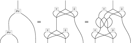
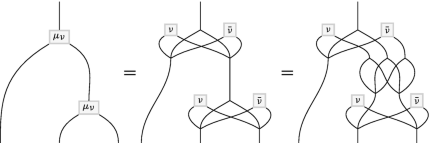
We have to check all the properties containing the product, i.e. the associativity, the unitality, the compatibility, and the compatibility of the product and the counit. The graphical notation

(5.10)

allows us to proceed purely graphically as follows. □

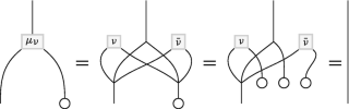
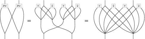
• (1) Associativity:

  

  (5.11)
  

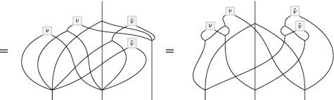
  and

  

  (5.12)
  

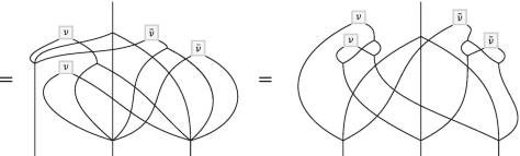
  We observe that the associativity for the twisted product is satisfied as a consequence of the cocycle relations (5.1) and (5.4). Notice that the diagrammatic calculations in (5.11) and (5.12) are mirror images of one another (with respect to a vertical mirror) accompanied with exchange of ν and $\bar \nu$.

• (2) Unitality:

  

  (5.13)
  

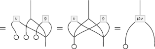
• (3) Compatibility:

  

  (5.14)
  

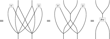
• (4) Compatibility of the twisted product with the counit:

  

  (5.15)

5.1.1 Dual Pairings

The algebraic properties of the evaluation form given by relations (4.2) and (4.3) can be formalized into the notion of a dual pairing. One can construct cocycles as dual pairings possessing an extra property.

Definition 5.2

A dual pairing between two bialgebras A and B is a linear form φ ∈ (A ⊗ B)^∗ such that

(5.16)

in the convolution algebra (A ⊗ A ⊗ B)^∗ and

(5.17)

in the convolution algebra (A ⊗ B ⊗ B)^∗,

(5.18)

and

(5.19)

where, in the graphical notation, the dotted lines correspond to A and solid lines to B.

Proposition 5.1

For any bialgebras A and B, a linear form φ ∈ (A ⊗ B)^∗ is a dual pairing between A and B if and only if one of the two following linear maps

$$\displaystyle \begin{aligned} l\colon A\to B^*,\ r\colon B\to A^*,\quad \langle l(a),b\rangle=\langle r(b),a\rangle=\langle\varphi, a\otimes b\rangle, \end{aligned} $$

(5.20)

factorizes through a bialgebra homomorphism into the corresponding restricted dual.

Proof

Assuming that φ is a dual pairing, we verify that l(A) ⊂ B^o and l: A → B^o is a homomorphism of bialgebras. To this end, we first derive the equalities

$$\displaystyle \begin{aligned} \mu_B^* l=(l\otimes l) \Delta_A,\quad \eta_B^* l=\epsilon_A \end{aligned} $$

(5.21)

which imply that l(A) ⊂ B^o and that l is a homomorphism of coalgebras. Using Sweedler’s sigma notation for the coproduct, see Sect. 1.7.2,

$$\displaystyle \begin{aligned} \Delta(a):= \sum_{(a)} a_{(1)}\otimes a_{(2)}, \end{aligned} $$

(5.22)

for any a ∈ A and α ⊗ β ∈ B^⊗2, we have

$$\displaystyle \begin{aligned} \begin{array}{rcl} {} & &\displaystyle \langle \mu_B^*(l(a)),\alpha\otimes \beta\rangle=\langle l(a),\alpha \beta \rangle=\langle \varphi,a\otimes \alpha \beta \rangle\\ & &\displaystyle \!=\!\sum_{(a)}\langle \varphi,a_{(1)}\otimes \alpha \rangle\langle\varphi,a_{(2)}\otimes \beta \rangle \!=\!\sum_{(a)}\langle l(a_{(1)}),\alpha \rangle\langle l(a_{(2)}),\beta \rangle\!=\!\langle( l\otimes l)(\Delta_A(a)),\alpha \otimes \beta \rangle, \end{array} \end{aligned} $$

(5.23)

obtaining the first equality of (5.21), and

$$\displaystyle \begin{aligned} \eta_B^*(l(a))=\langle l(a),\eta_B(1)\rangle=\langle \varphi,a\otimes \eta_B(1)\rangle=\epsilon_A(a), \end{aligned} $$

(5.24)

obtaining the second equality of (5.21).

Next, we show that

$$\displaystyle \begin{aligned} \Delta_B^* (l\otimes l)=l \mu_A,\quad l \eta_A=\epsilon_B^* \end{aligned} $$

(5.25)

which imply that l is a homomorphism of algebras. For any a ⊗ b ∈ A^⊗2 and α ∈ B, we have

$$\displaystyle \begin{aligned} \begin{array}{rcl} {} & &\displaystyle \langle( l \mu_A)(a\otimes b),\alpha\rangle=\langle l(ab),\alpha\rangle =\langle \varphi, ab\otimes \alpha\rangle\\ & &\displaystyle =\sum_{(\alpha)}\langle \varphi, a\otimes \alpha_{(1)}\rangle\langle \varphi, b\otimes \alpha_{(2)}\rangle =\sum_{(\alpha)}\langle l(a), \alpha_{(1)}\rangle\langle l(b), \alpha_{(2)}\rangle =\langle l(a)\otimes l(b),\Delta_B(\alpha)\rangle\\ \end{array} \end{aligned} $$

$$\displaystyle \begin{aligned} \begin{array}{rcl} & &\displaystyle =\langle\Delta_B^*(l(a)\otimes l(b)),\alpha\rangle, \end{array} \end{aligned} $$

(5.26)

obtaining the first equality of (5.25), and

$$\displaystyle \begin{aligned} \langle l(\eta_A(1)),\alpha\rangle=\langle \varphi, \eta_A(1)\otimes\alpha\rangle=\langle\epsilon_B,\alpha\rangle, \end{aligned} $$

(5.27)

obtaining the second equality of (5.25).

Assuming now the converse, i.e. that Eqs. (5.21) and (5.25) are satisfied, the calculations of (5.23), (5.24), (5.26), (5.27) reproduce the definition of a dual pairing.

The case where l is replaced with r is checked similarly. □

Proposition 5.2

For any bialgebra B, a convolution invertible dual pairing φ between B ^op and B (or, equivalently, between B and B ^cop ) is a cocycle on B if and only if

$$\displaystyle \begin{aligned} \varphi_{12}*\varphi_{23}=\varphi_{23}*\varphi_{12} \end{aligned} $$

(5.28)

in the convolution algebra $\left (B^{\otimes 3}\right )^*$.

Proof

Relations (5.16) and (5.17) take the form

$$\displaystyle \begin{aligned} \varphi (\mu_B\otimes\operatorname{id}_B)=\varphi_{23}*\varphi_{13} \end{aligned} $$

(5.29)

and

$$\displaystyle \begin{aligned} \varphi (\operatorname{id}_B\otimes\mu_B)=\varphi_{12}*\varphi_{13} \end{aligned} $$

(5.30)

so that (5.3) takes the form

$$\displaystyle \begin{aligned} \varphi_{12}*\varphi_{23}*\varphi_{13}=\varphi_{23}*\varphi_{12}*\varphi_{13}\Leftrightarrow \varphi_{12}*\varphi_{23}=\varphi_{23}*\varphi_{12}. \end{aligned} $$

(5.31)

□

5.2 Cobraided Bialgebras

Definition 5.3

A dual universal r-matrix in a bialgebra B = (B, μ,  Δ, η, 𝜖) is a convolution invertible element ρ ∈ (B ⊗ B)^∗ such that

(5.32)

(5.33)

(5.34)

A bialgebra provided with a dual universal r-matrix is called cobraided.

Exercise 5.3

Show that a dual universal r-matrix in a bialgebra B satisfies the following Yang–Baxter relation in the convolution algebra $\left (B^{\otimes 3}\right )^*$:

$$\displaystyle \begin{aligned} \rho_{1,2}*\rho_{1,3}*\rho_{2,3}=\rho_{2,3}*\rho_{1,3}*\rho_{1,2}. \end{aligned} $$

(5.35)

5.2.1 The Quantum Double

In this subsection, a Hopf algebra H will be drawn graphically by solid lines while its restricted dual H^o by dotted lines.

Proposition-Definition 5.2

Let H be a Hopf algebra. The quantum double D(H) of H is the bialgebra H ⊗ H^{o, op} twisted by the cocycle

(5.36)

It contains bialgebras H and H ^{o, op} as sub-bialgebras through the following canonical bialgebra embeddings:

(5.37)

and

(5.38)

If the antipode of H is invertible, then D(H) is a Hopf algebra. □

Proof

The proof boils down to straightforward verifications which are left as exercise. In particular, for the cocycle property, see Exercise 5.2. □

Exercise 5.4

Show that

(5.39)

where

(5.40)

Theorem 5.1

Let H be a Hopf algebra with invertible antipode. Then the restricted dual D(H)^o of the quantum double D(H) is a cobraided Hopf algebra with the following dual universal r-matrix

(5.41)

with the convolution inverse

(5.42)

where we use thick lines for the restricted dual D(H)^o and the graphical notation for the inverse of the antipode of H^o

Proof

Let us see first that $\bar \rho$ is a right inverse of ρ

That $\bar \rho$ is a left inverse of ρ is verified similarly.

In order to verify equality (5.32), we write it in an equivalent graphical form

(5.43)

where the equivalence is due to the fact that two linear forms on a vector space are equal if and only if they evaluate to one and the same value on any vector.

By using the definitions of ρ and the product of D(H)^o, we rewrite Eq. (5.43) in the form

(5.44)

Next, we can use the definition of the coproduct of D(H)^o in the bottom left parts of the diagrammatic equality (5.44) to obtain

(5.45)

where the units η_H can be eliminated by using the unitality axiom for H in the left hand side, and the definition of ψ in the right hand side

(5.46)

The obtained equality is a consequence of the equality (if two vectors are equal then their images by one and the same linear form are also equal)

(5.47)

which, in its turn, is equivalent to the equality (two linear forms on a vector space are equal if and only if they evaluate to one and the same value on any vector)

(5.48)

Now, in (5.48) we can use the definition of the product of H^o to obtain

(5.49)

By using the definitions of ψ in the left hand side and ı^o in the right hand side of (5.49), we obtain the equivalent equality

(5.50)

where we can further use the definitions of the (twice iterated) coproduct of H^o in the left hand side and the coproduct of D(H)^o in the right hand side to obtain

(5.51)

In (5.51), we can use the definition of ı^o in the left hand side and the unitality axiom for H^o in the right hand side to obtain

(5.52)

In (5.52), we can use the definitions of the coproduct of D(H)^o in the left hand side and of ψ in the right hand side to obtain

(5.53)

In the left hand side of (5.53), the definition of ψ and the composition of it with the unit of H^o lead to a simplification, while in the right hand side, the co-associativity properties of H and H^o and the duality allow to remove the antipode by the invertibility axiom. In this way, we obtain

(5.54)

In the left hand side of (5.54), the associativity and the co-associativity of H allow to remove the last antipode through the invertibility axiom for H. In this way, we obtain a tautological equality

(5.55)

Thus, equality (5.32) is proved.

Next, we verify equality (5.33)

(5.56)

Finally, we verify equality (5.34)

□

Remark 5.2

If H is a finite-dimensional Hopf algebra with a linear basis {e_i}_{i ∈ I} and {eⁱ}_{i ∈ I} is the dual linear basis of H^∗, then, the dual universal r-matrix is conjugate to the universal r-matrix

$$\displaystyle \begin{aligned} R:=\sum_{i\in I}\jmath e^i\otimes\imath e_i\in D(H)\otimes D(H) \end{aligned} $$

(5.57)

in the sense that, for any x, y ∈ (D(H))^o = (D(H))^∗, we have

$$\displaystyle \begin{aligned} \begin{array}{rcl} & &\displaystyle \langle x\otimes y,R\rangle=\sum_{i\in I}\langle x,\jmath e^i\rangle\langle y,\imath e_i\rangle=\sum_{i\in I}\langle x,\jmath e^i\rangle\langle \imath^o y,e_i\rangle\\ & &\displaystyle =\Big\langle x,\jmath\big(\sum_{i\in I}\langle \imath^oy,e_i\rangle e^i\big)\Big\rangle=\left\langle x,\jmath \imath^oy\right\rangle=\langle \varrho, x\otimes y\rangle. \end{array} \end{aligned} $$

(5.58)

In the infinite-dimensional case, formula (5.57) is formal but it is a convenient and useful tool for actual calculations.

5.3 The Quantum Double D(B_q)

In this section, we consider the example of the quantum group B_q described in Sect. 4.4 of Chap. 4. Recall that the parameter q there is generic, that it is not a root of unity.

Proposition 5.3

Let $q\in \mathbb {C}_{\ne 0}$ be such that $1\not \in q^{\mathbb {Z}_{\ne 0}}$. Then, the quantum double D(B_q) admits the following presentation:

$$\displaystyle \begin{aligned} \begin{array}{rcl} & &\displaystyle \mathbb{C}\big\langle a,b,\psi,\phi,\{\theta_z \}_{z\in\mathbb{C}_{\ne0}}\mid ab=qba,\\ & &\displaystyle \psi \theta_z =\theta_z \psi,\ \theta_z \theta_w=\theta_{zw}, \phi\psi-\psi\phi=\phi,\ \phi \theta_z =z \theta_z \phi,\\ & &\displaystyle \psi a=a\psi,\ \psi b-b\psi=b,\ \theta_z a=a\theta_z ,\ \theta_z b=z b\theta_z ,\\ & &\displaystyle \phi a=qa\phi,\ \phi b-q b\phi=(1-q)(1-a\theta_q);\\ & &\displaystyle \Delta a=a\otimes a,\ \Delta b=a\otimes b+b\otimes 1,\\ & &\displaystyle \Delta \psi=\psi\otimes 1+1\otimes\psi,\ \Delta\theta_z =\theta_z \otimes \theta_z ,\ \Delta \phi=\theta_q\otimes\phi+\phi\otimes 1\big\rangle \end{array} \end{aligned} $$

(5.59)

Proof

As the first two lines and the last two lines in the presentation are just the presentations of the Hopf sub-algebras B_q and $B_q^{o,\text{op}}$ put together, we need to check only the relations in the third and forth lines. These are relations between the generators of B_q and $B_q^{o,\text{op}}$ which are of the form

$$\displaystyle \begin{aligned} (\jmath f)(\imath x)=\sum_{(f),(x)}\langle f_{(1)},x_{(1)}\rangle (\imath x_{(2)}) (\jmath f_{(2)}) \langle f_{(3)},S x_{(3)}\rangle, \quad x\in B_q,\ f\in B_q^{o,\text{op}}. \end{aligned} $$

(5.60)

By writing informally just x instead of ıx and f instead of ȷf, let us write out these relations one after another for x ∈{a, b} and f ∈{ψ, θ_z, ϕ} by using the iterated coproducts

$$\displaystyle \begin{aligned} \Delta^{(3)}a=a\otimes a\otimes a,\quad \Delta^{(3)}b=b\otimes 1\otimes 1+a\otimes b\otimes 1+a\otimes a\otimes b \end{aligned} $$

(5.61)

and

$$\displaystyle \begin{aligned} \begin{array}{rcl} {} & &\displaystyle \Delta^{(3)}\psi=\psi\otimes \epsilon\otimes \epsilon+\epsilon\otimes \psi\otimes \epsilon+\epsilon\otimes \epsilon\otimes \psi,\quad \Delta^{(3)}\theta_z=\theta_z\otimes \theta_z\otimes \theta_z,\\ & &\displaystyle \Delta^{(3)}\phi=\phi\otimes \epsilon\otimes \epsilon+\theta_q\otimes \phi\otimes \epsilon+\theta_q\otimes \theta_q\otimes \phi. \end{array} \end{aligned} $$

(5.62)

The Case (f = ψ, x = a) The first coproducts in (5.61) and (5.62) imply that relation (5.60) takes the form

$$\displaystyle \begin{aligned} \psi a\!=\!\langle \psi,a\rangle a \langle \epsilon,a^{-1}\rangle+\langle \epsilon,a\rangle a\psi \langle \epsilon,a^{-1}\rangle+\langle \epsilon,a\rangle a \langle \psi,a^{-1}\rangle \!=\! a+ a\psi-a=a\psi. \end{aligned} $$

(5.63)

The Case (f = ψ, x = b) The second coproduct in (5.61) and the first one in (5.62) imply that

$$\displaystyle \begin{aligned} \begin{array}{rcl} & &\displaystyle \psi b=\langle \psi,b\rangle 1 \langle \epsilon,1\rangle+\langle \psi ,a\rangle b \langle \epsilon,1\rangle+\langle \psi,a\rangle a \langle \epsilon,-a^{-1}b\rangle\\ & &\displaystyle +\langle \epsilon,b\rangle \psi \langle \epsilon,1\rangle+\langle \epsilon ,a\rangle b\psi \langle \epsilon,1\rangle+\langle \epsilon,a\rangle a\psi \langle \epsilon,-a^{-1}b\rangle\\ & &\displaystyle \langle \epsilon,b\rangle 1 \langle \psi,1\rangle+\langle \epsilon ,a\rangle b \langle \psi,1\rangle+\langle \epsilon,a\rangle a \langle \psi,-a^{-1}b\rangle\\ & &\displaystyle =(0+ b+0)+(0+b\psi+0)+(0+0+0)=b+b\psi. \end{array} \end{aligned} $$

(5.64)

The Case (f = θ_z, x = a) The first coproduct in (5.61) and the second one in (5.62) imply that

$$\displaystyle \begin{aligned} \theta_za=\langle \theta_z,a\rangle a\theta_z \langle \theta_z,a^{-1}\rangle=z a\theta_z z^{-1}= a\theta_z. \end{aligned} $$

(5.65)

The Case (f = θ_z, x = b) The second coproducts in (5.61) and (5.62) imply that

$$\displaystyle \begin{aligned} \begin{array}{rcl} & &\displaystyle \theta_zb=\langle \theta_z,b\rangle \theta_z \langle \theta_z,1\rangle+\langle \theta_z,a\rangle b\theta_z \langle \theta_z,1\rangle+\langle \theta_z,a\rangle a\theta_z \langle \theta_z,-a^{-1}b\rangle\\ & &\displaystyle =0+z b\theta_z +0= zb\theta_z. \end{array} \end{aligned} $$

(5.66)

The Case (f = ϕ, x = a) The first coproduct in (5.61) and the third one in (5.62) imply that

$$\displaystyle \begin{aligned} \begin{array}{rcl} & &\displaystyle \phi a=\langle \phi,a\rangle a \langle \epsilon,a^{-1}\rangle+\langle \theta_q,a\rangle a\phi \langle \epsilon,a^{-1}\rangle+\langle \theta_q,a\rangle a\theta_q \langle \phi,a^{-1}\rangle\\ & &\displaystyle =0+q a\phi +0= q a\phi . \end{array} \end{aligned} $$

(5.67)

The Case (f = ϕ, x = b) The second coproduct in (5.61) and the third one in (5.62) imply that

$$\displaystyle \begin{aligned} \begin{array}{rcl} & &\displaystyle \phi b=\langle \phi,b\rangle 1 \langle \epsilon,1\rangle+\langle \phi,a\rangle b \langle \epsilon,1\rangle+\langle \phi,a\rangle a \langle \epsilon,-a^{-1}b\rangle\\ & &\displaystyle +\langle \theta_q,b\rangle \phi \langle \epsilon,1\rangle+\langle \theta_q,a\rangle b\phi \langle \epsilon,1\rangle+\langle \theta_q,a\rangle a\phi \langle \epsilon,-a^{-1}b\rangle\\ & &\displaystyle +\langle \theta_q,b\rangle \theta_q \langle \phi,1\rangle+\langle \theta_q,a\rangle b\theta_q \langle \phi,1\rangle+\langle \theta_q,a\rangle a\theta_q \langle \phi,-a^{-1}b\rangle\\ & &\displaystyle =((1-q)1+0+0)+(0+q b\phi +0)+(0+0+qa\theta_q\langle\theta_q,-a^{-1}\rangle\langle \phi,b\rangle)\\ & &\displaystyle = (1-q)1+q b\phi-a\theta_q(1-q)=(1-q)(1-a\theta_q)+q b\phi . \end{array} \end{aligned} $$

(5.68)

□

5.3.1 Irreducible Representations of D(B_q)

Proposition 5.4

The elements c, d ∈ D(B_q) defined by the relations

$$\displaystyle \begin{aligned} c\theta_q=a \end{aligned} $$

(5.69)

and

$$\displaystyle \begin{aligned} \phi b-1-q a \theta_q =\theta_qd=qb\phi-q-a\theta_q \end{aligned} $$

(5.70)

are central.

Proof

That the element c is central is an easy check. To see that d is central, we define two elements w, w′∈ D(B_q) by the relations

$$\displaystyle \begin{aligned} \phi b=u+v a \theta_q +w,\quad qb\phi=u'+v'a\theta_q+w', \end{aligned} $$

(5.71)

where $u,u',v,v'\in \mathbb {C}$ are fixed as follows. First, we impose two conditions

$$\displaystyle \begin{aligned} u-u'=1-q=v'-v \end{aligned} $$

(5.72)

which, due to the defining relation between b and ϕ, imply that w′ = w. By straightforward verifications one sees that w commutes with a, ψ and θ_z for all $z\in \mathbb {C}_{\ne 0}$. Next, we have the equalities

$$\displaystyle \begin{aligned} u'b+v'a\theta_q b+wb=qb\phi b=qbu+qbva\theta_q+qbw \end{aligned} $$

(5.73)

which, under two more relations of the form

$$\displaystyle \begin{aligned} u'=qu,\quad qv'=v, \end{aligned} $$

(5.74)

imply that wb = qbw. The system of Eqs. (5.72) and (5.74) on unknowns u, u′, v, v′ admits a unique solution

$$\displaystyle \begin{aligned} u=1=v',\quad u'=q=v. \end{aligned} $$

(5.75)

Now, it is an easy check that ϕw = qwϕ. Indeed, we have

$$\displaystyle \begin{aligned} \begin{array}{rcl} & &\displaystyle \phi w=\phi(qb\phi-q-a\theta_q)= q\phi b\phi-q\phi-\phi a \theta_q\\ & &\displaystyle =q\phi b\phi-q\phi-q^2 a \theta_q\phi=q(\phi b-1-q a \theta_q)\phi=qw\phi. \end{array} \end{aligned} $$

(5.76)

Finally, the equality w = θ_qd, together with the obtained commutation relations for w, implies that d is central. □

Proposition 5.5

Let $q\in \mathbb {C}_{\ne 0}$ be such that $1\not \in q^{\mathbb {Z}_{\ne 0}}$. The center of the algebra D(B_q) coincides with the polynomial subalgebra $\mathbb {C}[c,c^{-1},d]$ where c and d are defined in (5.69) and (5.70)

Proof

By Proposition 5.4, for any n ∈ ω, one can easily verify by recurrence the equality

$$\displaystyle \begin{aligned} \phi^nb^n=\prod_{k\in n}(1+q^k \theta_q d+q^{2k+1}\theta_q^2 c). \end{aligned} $$

(5.77)

This means that any element x ∈ D(B_q) can uniquely be written in the form

$$\displaystyle \begin{aligned} x=\sum_{(u,m)\in \mathbb{C}_{\ne0}\times \mathbb{Z}}\theta_{u} e_m p_{u,m}(c,d,\psi), \end{aligned} $$

(5.78)

where

$$\displaystyle \begin{aligned} e_m:=\left\{ \begin{array}{cc} b^m & \text{if }\ m>0; \\ 1 & \text{if }\ m=0; \\ \phi^{-m} & \text{if }\ m<0 \end{array} \right. \end{aligned} $$

(5.79)

and $p_{u,m}(a,c,\psi )\in \mathbb {C}[c,c^{-1},d,\psi ]$ is non-zero for only finitely many pairs (u, m). Remark that, for any $m\in \mathbb {Z}$, the element e_m satisfies the relations

$$\displaystyle \begin{aligned} \psi e_m=e_m(\psi+m),\quad \theta_ze_m=z^me_m\theta_z\quad \forall z\in\mathbb{C}_{\ne0}. \end{aligned} $$

(5.80)

Assume that x is central. Then, for any $z\in \mathbb {C}_{\ne 0}$, we have the equality

$$\displaystyle \begin{aligned} x=\theta_{z} x \theta_{z}^{-1}=\sum_{(u,m)\in \mathbb{C}_{\ne0}\times \mathbb{Z}}\theta_{u} e_m z^m p_{u,m}(c,d,\psi) \end{aligned} $$

(5.81)

which implies that for any fixed pair $(u,m)\in \mathbb {C}_{\ne 0}\times \mathbb {Z}$, one has the family of equalities

$$\displaystyle \begin{aligned} p_{u,m}=z^m p_{u,m}\quad \forall z\in\mathbb{C}_{\ne0}. \end{aligned} $$

(5.82)

This means that p_u,m can only be non-zero if m = 0. Thus, the element x takes the form

$$\displaystyle \begin{aligned} x=\sum_{u\in\mathbb{C}_{\ne0}}\theta_{u} p_{u,0}(c,d,\psi). \end{aligned} $$

(5.83)

The equality

$$\displaystyle \begin{aligned} bx=xb=b\sum_{u\in\mathbb{C}_{\ne0}}\theta_{u} up_{u,0}(a,c,\psi+1) \end{aligned} $$

(5.84)

is equivalent to the equalities

$$\displaystyle \begin{aligned} up_{u,0}(c,d,\psi+1)=p_{u,0}(c,d,\psi) \quad \forall u\in \mathbb{C}_{\ne0} \end{aligned} $$

(5.85)

which imply that the polynomial p_u,0(a, c, ψ) can be non-zero only if u = 1 and if it does not depend on ψ. We conclude that $x=p_{1,0}(c,d)\in \mathbb {C}[c,c^{-1},d]$. □

Theorem 5.2

Let $q\in \mathbb {C}$ be such that $1\not \in q^{\mathbb {Z}_{\ne 0}}$ . Then, any finite dimensional irreducible representation $\lambda \colon D(B_q)\to \operatorname {End}(V)$ is characterized by the dimension $N:=\operatorname {dim}(V)\in \mathbb {Z}_{>0}$ , a complex number $\gamma \in \mathbb {C}$ , and a multiplicative group homomorphism $\xi \colon \mathbb {C}_{\ne 0}\to \mathbb {C}_{\ne 0}$ such that there exists a linear basis $\{v_n\}_{n\in \underline {N}}$ of V  satisfying the relations

$$\displaystyle \begin{aligned} \begin{array}{rcl} {} & &\displaystyle (\lambda a)v_n=q^{N-1-n}\xi_q^{-1}v_n,\quad (\lambda \psi) v_n=(\gamma-n)v_n,\quad (\lambda\theta_z ) v_n=z^{-n}\xi_zv_n,\\ & &\displaystyle (\lambda b)v_n=(1-q^{-n})v_{n-1},\quad (\lambda\phi) v_n=(1-q^{N-n-1})v_{n+1}. \end{array} \end{aligned} $$

(5.86)

Proof

To simplify notation, we will write $\hat x$ instead of λx for any x ∈ D(B_q), and [x, y] instead of xy − yx.

As in an irreducible representation all central elements are realised by scalars, there exist $\alpha \in \mathbb {C}_{\ne 0}$ and $\beta \in \mathbb {C}$ such that the central elements c and d defined in (5.69) and (5.70) are represented by scalar multiples of the identity operator:

$$\displaystyle \begin{aligned} \hat c=\alpha\operatorname{id}_V,\quad \hat d=\beta\operatorname{id}_V. \end{aligned} $$

(5.87)

Let u′∈ V ∖{0} be an eigenvector of $\hat \psi$ corresponding to an eigenvalue $\gamma '\in \mathbb {C}$. Then, the vector $\hat bu'$ either vanishes or it is an eigenvector of $\hat \psi$ corresponding to the eigenvalue γ′ + 1. Indeed,

$$\displaystyle \begin{aligned} \hat\psi \hat bu'=([\hat\psi, \hat b]+\hat b\hat\psi)u'=\hat b(1+\hat\psi)u'=(\gamma'+1)bu'. \end{aligned} $$

(5.88)

Iterating the action of $\hat b$ and taking into account the fact that $\operatorname {dim}(V)<\infty$, we conclude that there exists a positive integer K such that $u'':= \hat b^{K-1}u'\ne 0$ and

$$\displaystyle \begin{aligned} \hat bu''= 0,\quad \hat \psi u''=\gamma u'',\quad \gamma:= \gamma'+K-1. \end{aligned} $$

(5.89)

Additionally, as the elements $\{\theta _z\}_{z\in \mathbb {C}_{\ne 0}}$ and ψ generate a commutative sub-algebra A of D(B_q), and any irreducible finite dimensional representation of a commutative algebra is one dimensional, there exists a non zero vector u ∈ λ(A)u″ that generates an irreducible sub-representation of A. This means that the following relations are satisfied:

$$\displaystyle \begin{aligned} \hat bu= 0,\quad \hat\psi u=\gamma u,\quad \hat\theta_zu=\xi_zu,\quad \forall z\in \mathbb{C}_{\ne0}, \end{aligned} $$

(5.90)

where

$$\displaystyle \begin{aligned} \xi\colon \mathbb{C}_{\ne0}\to \mathbb{C}_{\ne0} \end{aligned} $$

(5.91)

is a (multiplicative) group homomorphism.

By a similar reasoning, as in the case of the vector u′ above, for any n ∈ ω, the vector $\hat \phi ^nu$ either vanishes or it is an eigenvector of $\hat \psi$ corresponding to the eigenvalue γ − n, and, as $\operatorname {dim}(V)<\infty$, there exists a positive integer M such that

$$\displaystyle \begin{aligned} \hat \phi^{M-1}u\ne 0,\quad \hat\phi^Mu=0. \end{aligned} $$

(5.92)

We denote by W the linear span of the vectors $\{\hat \phi ^nu\}_{n\in \underline {M}}$. Let us show that W = V .

First, we note that, apart from the relations

$$\displaystyle \begin{aligned} \hat \psi \hat\phi^nu=(\gamma-n)\hat\phi^nu,\quad n\in \underline{M}, \end{aligned} $$

(5.93)

we also have

$$\displaystyle \begin{aligned} \check\theta_z\hat\phi^nu=z^{-n} \hat\phi^nu,\quad n\in \underline{M}, \end{aligned} $$

(5.94)

where we have denoted

$$\displaystyle \begin{aligned} \check\theta_z:=\hat\theta_z/\xi_z,\quad \forall z\in\mathbb{C}_{\ne0}. \end{aligned} $$

(5.95)

Next, by using (5.87) in (5.70), we obtain

$$\displaystyle \begin{aligned} \hat\phi\hat b=\operatorname{id}_V+\beta \hat\theta_q+q\alpha \hat\theta_{q}^2 \end{aligned} $$

(5.96)

and

$$\displaystyle \begin{aligned} \hat b\hat\phi=\operatorname{id}_V+q^{-1}\beta \hat\theta_q+q^{-1}\alpha \hat\theta_q^2 \end{aligned} $$

(5.97)

Applying (5.96) to u and (5.97) to $\hat \phi ^{M-1}u$, and taking into account relations (5.90), (5.92) and (5.94), we obtain

$$\displaystyle \begin{aligned} (1+\beta\xi_q+q\alpha \xi_q^2)u=0\Rightarrow 1+\beta\xi_q+\alpha q\xi_q^2=0 \end{aligned} $$

(5.98)

and

$$\displaystyle \begin{aligned} (1+\beta q^{-M}\xi_q+\alpha q^{1-2M}\xi_q^2)\hat\phi^{M-1}u=0\Rightarrow 1+\beta q^{-M}\xi_q+\alpha q^{1-2M}\xi_q^2=0. \end{aligned} $$

(5.99)

Excluding β from (5.98) and (5.99), we obtain

$$\displaystyle \begin{aligned} (1-\alpha q^{1-M}\xi_q^2)(1-q^{M})=0\Leftrightarrow \alpha=q^{M-1}\xi_q^{-2} \end{aligned} $$

(5.100)

and also from (5.98) it follows that

$$\displaystyle \begin{aligned} \beta=-\xi_q^{-1}(1+q^{M}). \end{aligned} $$

(5.101)

By using substitutions (5.100), (5.101) and notation (5.95), we rewrite (5.96) and (5.97) as follows:

$$\displaystyle \begin{aligned} \hat\phi\hat b=\operatorname{id}_V-(1+q^M)\check\theta_q+q^{M}\check\theta_q^2 =(\operatorname{id}_V-\check\theta_q)(\operatorname{id}_V-q^{M}\check\theta_q) \end{aligned} $$

(5.102)

and

$$\displaystyle \begin{aligned} \hat b\hat\phi=\operatorname{id}_V-(1+q^M)q^{-1}\check\theta_q+q^{M-2}\check\theta_q^2 =(\operatorname{id}_V-q^{-1}\check\theta_q)(\operatorname{id}_V-q^{M-1}\check\theta_q). \end{aligned} $$

(5.103)

For $n\in \underline {M}\setminus \{0\}$, applying relation (5.103) to the vector $\hat \phi ^{n-1}u$ and taking into account (5.94), we obtain

$$\displaystyle \begin{aligned} \hat b\hat\phi^{n}u=(1-q^{-n})(1-q^{M-n})\hat\phi^{n-1}u. \end{aligned} $$

(5.104)

Thus, we conclude that the subspace W of V  generated by vectors $\{\hat \phi ^nu\}_{n\in \underline {M}}$ is an invariant subspace of the representation λ, and by the irreducibility of λ, we conclude that W = V  so that

$$\displaystyle \begin{aligned} N:=\operatorname{dim}(V)=\operatorname{dim}(W)=M, \end{aligned} $$

(5.105)

and the vectors $\{\hat \phi ^nu\}_{n\in \underline {M}}$ form a linear basis of V .

Let us define renormalized vectors

$$\displaystyle \begin{aligned} v_n:=(q)_{N-n-1}\hat\phi^nu,\quad n\in \underline{N}. \end{aligned} $$

(5.106)

Then, by using the relation

$$\displaystyle \begin{aligned} (1-q^k)(q)_{k-1}=(q)_{k},\quad \forall k\in\mathbb{Z}_{>0}, \end{aligned} $$

(5.107)

we have

$$\displaystyle \begin{aligned} \hat bv_n=(q)_{N-n-1}(1-q^{-n})(1-q^{N-n})\hat\phi^{n-1}u=(1-q^{-n})v_{n-1} \end{aligned} $$

(5.108)

and

$$\displaystyle \begin{aligned} \hat\phi v_n=(q)_{N-n-1}\hat\phi^{n+1}v=(1-q^{N-n-1})v_{n+1}. \end{aligned} $$

(5.109)

□

Remark 5.3

The vanishing properties of the coefficients of relations (5.108) with n = 0 and (5.109) with n = N − 1 naturally take care of the annihilation relations

$$\displaystyle \begin{aligned} \hat bv_0=\hat\phi v_{N-1}=0. \end{aligned} $$

(5.110)

Exercise 5.5

For any $n\in \underline {N}$, show that

$$\displaystyle \begin{aligned} \hat b^kv_n=(q^{-n};q)_kv_{n-k},\quad \forall k\in \underline{n+1}, \end{aligned} $$

(5.111)

and

$$\displaystyle \begin{aligned} \hat\phi^kv_n=(q^{N-n-k};q)_kv_{n+k},\quad \forall k\in \underline{N-n}. \end{aligned} $$

(5.112)

with the notation

$$\displaystyle \begin{aligned} (x;q)_n:= \begin{cases} \prod_{k=0}^{n-1}(1-xq^k)&\text{if } k>0;\\ 1&\text{if } k=0. \end{cases} \end{aligned} $$

(5.113)

5.3.2 Quantum Group U_q(sl₂)

Recall that the element $c:=a\theta _{q}^{-1}\in D(B_{q})$ is central and grouplike. This means that the vector subspace

$$\displaystyle \begin{aligned} I_q:=(c-1)D(B_{q})\subset D(B_{q})\end{aligned}$$

is a bi-ideal stable under the action of the antipode, see Definitions 2.6, 2.2 and 2.4. By the results of Chap. 2, Sect. 2.4.2, we conclude that the quotient vector space

$$\displaystyle \begin{aligned} H_q:=D(B_{q})/I_q\end{aligned}$$

admits a unique structure of a Hopf algebra such that the canonical projection map π: D(B_q) → H_q is a morphism of Hopf algebras. The Hopf algebra H_q is closely related with the quantum group U_q(sl₂) which is defined by the following presentation:

$$\displaystyle \begin{aligned} & \text{generators: } k,e,f;\\ & \text{relations: } ke=q^2ek,\quad kf=q^{-2}fk,\quad ef-fe =\frac{k-k^{-1}}{q-q^{-1}}\\ &\text{coproducts: } \Delta k=k\otimes k,\quad \Delta e=k\otimes e+e\otimes 1,\quad \Delta f=1\otimes f+f\otimes k^{-1} \end{aligned} $$

where we assume that q²≠1 and k is invertible (as a group-like element in any Hopf algebra).

Exercise 5.6

Determine $\alpha ,\beta \in \mathbb {C}_{\ne 0}$ such that the map

$$\displaystyle \begin{aligned} k\mapsto a+I_{q^2},\quad e\mapsto \alpha b+I_{q^2},\quad f\mapsto \beta a^{-1}\phi+I_{q^2} \end{aligned}$$

extends to an injective morphism of Hopf algebras $h\colon U_q(sl_2)\to H_{q^2}$.

The algebra U_q(sl₂) was discovered in [24], and the general theory of quantum groups has been subsequently developed in the works [11, 13, 17]. An introduction for this subject can be found in the book [16].

5.4 The Hopf Algebra D(B₁)

Let B₁ be the commutative Hopf algebra over $\mathbb {C}$ corresponding to the quantum group B_q with q = 1 defined and analyzed in Sect. 4.4 of Chap. 4 in the case of generic q, that is when q is not a root of unity. Here, we consider the case of the simplest root of unity q = 1. This Hopf algebra coincides with J₀, the specification of J_ħ to ħ = 0, see Sect. 4.3 of Chap. 4. In Sect. 6.5 of Chap. 6, this algebra will be used for interpretation of the Alexander polynomial of knots as an example of a universal invariant. For this reason, below we briefly describe the restricted dual and the quantum double of B₁, leaving the detailed analysis to exercises.

5.4.1 The Restricted Dual Hopf Algebra $B_1^{o,\text{op}}$

The opposite $B_1^{o,\text{op}}$ of the restricted dual Hopf algebra $B_1^o$ is composed of two Hopf subalgebras: the group algebra $\mathbb {C}[\operatorname {Aff}_1(\mathbb {C})]$ generated by group-like elements

$$\displaystyle \begin{aligned} \chi_{u,v},\quad (u,v)\in \mathbb{C}\times\mathbb{C}_{\ne0},\quad \chi_{u,v}\chi_{u',v'}=\chi_{u+vu',vv'}, \end{aligned} $$

(5.114)

and the universal enveloping algebra $U(\operatorname {Lie}\operatorname {Aff}_1(\mathbb {C}))$ generated by two primitive elements ψ and ϕ satisfying the relation

$$\displaystyle \begin{aligned} \phi\psi-\psi\phi=\phi. \end{aligned} $$

(5.115)

The relations between the generators of $\mathbb {C}[\operatorname {Aff}_1(\mathbb {C})]$ and $U(\operatorname {Lie}\operatorname {Aff}_1(\mathbb {C}))$ are of the form

$$\displaystyle \begin{aligned}{}[\chi_{u,v},\psi]=u\phi \chi_{u,v},\quad \chi_{u,v} \phi =v\phi\chi_{u,v}\quad \forall (u,v)\in \mathbb{C}\times\mathbb{C}_{\ne0} \end{aligned} $$

(5.116)

where [x, y] := xy − yx. As linear forms on B₁, they are defined by the relations

$$\displaystyle \begin{aligned} \begin{array}{rcl} & &\displaystyle \langle\chi_{u,v},b^ma^n\rangle=u^mv^{-m-n},\\ & &\displaystyle \langle\phi,b^ma^n\rangle=\delta_{m,1}, \quad \langle\psi,b^ma^n\rangle=\delta_{m,0}n,\quad \forall(m,n)\in\mathbb{Z}_{\ge0}\times \mathbb{Z}. \end{array} \end{aligned} $$

(5.117)

Exercise 5.7

By using the methods of Chap. 4, provide the details of the above description of the structure of the Hopf algebra $B_1^{o,\text{op}}$.

5.4.2 The Quantum Double D(B₁)

The commutation relations (5.60) in the case of the quantum double D(B₁) take the form

$$\displaystyle \begin{aligned} \begin{array}{rcl} {} & &\displaystyle [\psi,b]=b,\quad [\phi,b]=1-a,\\ & &\displaystyle b\chi_{u,v} =\chi_{u,v}(bv+(a-1)u)\quad \forall (u,v)\in \mathbb{C}\times\mathbb{C}_{\ne0} \end{array} \end{aligned} $$

(5.118)

and a is central.

Exercise 5.8

Prove the defining relations of D(B₁) given by Eq. (5.118).

Exercise 5.9

Show that in any finite-dimensional representation of the algebra D(B₁), the elements 1 − a, b and ϕ are nilpotent.

The formal universal r-matrix of D(B₁), see Remark 5.2, is given by the formula

$$\displaystyle \begin{aligned} R:=(1\otimes{a})^{{\psi}\otimes 1}e^{{\phi}\otimes{b}}=\sum_{m,n\ge0}\frac 1{n!}\binom{{\psi}}{m}{\phi}^n\otimes ({a}-1)^m {b}^n \end{aligned} $$

(5.119)

and it is well defined in the context of finite-dimensional representations for the following reason.

Any finite dimensional right comodule V  over (D(B₁))^o is a left module over D(B₁) defined by

$$\displaystyle \begin{aligned} xv=\sum_{(v)}v_{(0)}\langle v_{(1)},x\rangle,\quad \forall (x,v)\in D(B_1)\times V \end{aligned} $$

(5.120)

where we extend Sweedler’s sigma notation to comodules. Thus, it suffices to make sense of formula (5.119) in the case of an arbirary finite-dimensional representation of D(B₁) where the elements 1 − a, b and ϕ are necessarily nilpotent, so that the formal infinite double sum truncates to a well defined finite sum.

5.4.3 The Center of D(B₁)

Proposition 5.6

The center of the algebra D(B₁) is the polynomial subalgebra $\mathbb {C}[a^{\pm 1},c]$ where

$$\displaystyle \begin{aligned} c:=\phi b+(a-1)\psi. \end{aligned} $$

(5.121)

Proof

It is easily verified that c is central. Any element x ∈ D(B₁) can uniquely be written in the form

$$\displaystyle \begin{aligned} x=\sum_{(u,v,m)\in \mathbb{C}\times \mathbb{C}_{\ne0}\times \mathbb{Z}}\chi_{u,v} e_m p_{u,v,m}(a,c,\psi), \end{aligned} $$

(5.122)

where

$$\displaystyle \begin{aligned} e_m:=\left\{ \begin{array}{cc} b^m & \text{if }\ m>0; \\ 1 & \text{if }\ m=0; \\ \phi^{-m} & \text{if }\ m<0 \end{array} \right. \end{aligned} $$

(5.123)

and the polynomial $p_{u,v,m}(a,c,\psi )\in \mathbb {C}[a^{\pm 1},c,\psi ]$ is non-zero for only finitely many triples (u, v, m).

Assume that x ∈ D(B₁) is a central element. Then, for any $s\in \mathbb {C}_{\ne 0}$, we have the equality

$$\displaystyle \begin{aligned} \begin{array}{rcl} & &\displaystyle x=\chi_{0,s}^{-1} x \chi_{0,s}=\sum_{(u,v,m)\in \mathbb{C}\times \mathbb{C}_{\ne0}\times \mathbb{Z}}\chi_{u/s,v} e_m s^m p_{u,v,m}(a,c,\psi)\\ & &\displaystyle =\sum_{(u,v,m)\in \mathbb{C}\times \mathbb{C}_{\ne0}\times \mathbb{Z}}\chi_{u,v} e_m s^m p_{us,v,m}(a,c,\psi) \end{array} \end{aligned} $$

(5.124)

which implies that for any fixed triple $(u,v,m)\in \mathbb {C}\times \mathbb {C}_{\ne 0}\times \mathbb {Z}$, one has the family of equalities

$$\displaystyle \begin{aligned} p_{u,v,m}=s^m p_{us,v,m}\quad \forall s\in\mathbb{C}_{\ne0}. \end{aligned} $$

(5.125)

This means that p_u,v,m can only be non-zero if u = m = 0. Thus, the element x takes the form

$$\displaystyle \begin{aligned} x=\sum_{v\in\mathbb{C}_{\ne0}}\chi_{0,v} p_{0,v,0}(a,c,\psi). \end{aligned} $$

(5.126)

The equality

$$\displaystyle \begin{aligned} bx=xb=b\sum_{v\in\mathbb{C}_{\ne0}}\chi_{0,v} v^{-1}p_{0,v,0}(a,c,\psi+1). \end{aligned} $$

(5.127)

is equivalent to the equalities

$$\displaystyle \begin{aligned} p_{0,v,0}(a,c,\psi+1)=v^{-1}p_{0,v,0}(a,c,\psi) \quad \forall v\in \mathbb{C}_{\ne0} \end{aligned} $$

(5.128)

which imply that the polynomial p_0,v,0(a, c, ψ) can be non-zero only if v = 1 and if it does not depend on ψ. We conclude that $x\in \mathbb {C}[a^{\pm 1},c]$. □

5.5 Solutions of the Yang–Baxter Equation

Definition 5.4

An r-matrix over a coalgebra C is an invertible element ρ of the convolution algebra (C^⊗2)^∗ such that the following Yang–Baxter equation is satisfied in the convolution algebra (C^⊗3)^∗:

$$\displaystyle \begin{aligned} \rho_{1,2}*\rho_{1,3}*\rho_{2,3}=\rho_{2,3}*\rho_{1,3}*\rho_{1,2}. \end{aligned} $$

(5.129)

Example 5.1

The dual universal r-matrix of a cobraided bialgebra B is an r-matrix over the underlying coalgebra of B. □

Definition 5.5

An r-matrix over a vector space V is an element $r\in \operatorname {Aut}(V^{\otimes 2})$ such that the following Yang–Baxter equation is satisfied in the algebra $\operatorname {End}(V^{\otimes 3})$:

$$\displaystyle \begin{aligned} r_{1,2} r_{2,3}r_{1,2}=r_{2,3}r_{1,2}r_{2,3},\quad r_{1,2}:=r\otimes\operatorname{id}_V,\quad r_{2,3}:=\operatorname{id}_V\otimes r. \end{aligned} $$

(5.130)

By using the graphical notation , the Yang–Baxter equation (5.130) takes the following graphical form

(5.131)

In the particular case, where V  is a finite dimensional vector space over a field $\mathbb {F}$, let B ⊂ V  be a linear basis. Defining the matrix coefficients

$$\displaystyle \begin{aligned} \big\{r_{a,b}^{c,d}\mid a,b,c,d\in B\big\}\subset\mathbb{F},\quad r(a\otimes b)=\sum_{c,d\in B}r_{a,b}^{c,d} c\otimes d ,\quad a,b\in B, \end{aligned} $$

(5.132)

we reduce the Yang–Baxter equation (5.131) to a over determined system of non-linear polynomial equations

$$\displaystyle \begin{aligned} \sum_{s,t,u\in B}r^{i,j}_{u,s}r^{s,k}_{t,n}r^{u,t}_{l,m}=\sum_{s,t,u\in B}r^{j,k}_{s,u}r^{i,s}_{l,t}r^{t,u}_{m,n},\quad i,j,k,l,m,n\in B, \end{aligned} $$

(5.133)

which can also be represented in a graphical form by assigning elements of the basis B to edges in (5.131) and summing over the elements assigned to the internal edges

(5.134)

with the identifications

(5.135)

Proposition 5.7

Let V = (V, δ: V → V ⊗ C) be a right comodule over a coalgebra C, and ρ ∈ (C^⊗2)^∗ an r-matrix over the coalgebra C. Then, the element

(5.136)

is an r-matrix over the vector space V . Here, in the graphical description, the thick lines correspond to V  and thin lines to C.

Proof

The inverse r⁻¹ of r is given by the formula (exercise)

(5.137)

where $\bar \rho$ is the convolution inverse of ρ.

By using three times the equality $(\delta \otimes \operatorname {id}_C)\delta =(\operatorname {id}_V\otimes \Delta )$, we transform the left hand side of (5.130) as follows:

(5.138)

and, doing a similar calculation for the right hand side of (5.130), we obtain

(5.139)

thus concluding that Eq. (5.130) is satisfied due to the convolutional Yang–Baxter equality (5.129) for the r-matrix ρ over the coalgebra C. □

The following proposition allows one to view any finite dimensional module over an algebra as a comodule over the restricted dual of that algebra. In this way, one can associate to any finite dimensional representation of a quantum double an r-matrix over the vector space underlying that representation.

Proposition 5.8

Let V  be a finite dimensional left module over an algebra A, and B ⊂ V  a linear basis. Then, V  is a right comodule over the coalgebra A^o with the coaction

$$\displaystyle \begin{aligned} \delta b=\sum_{b'\in B}b'\otimes \lambda_{b',b} \end{aligned} $$

(5.140)

where $\{ \lambda _{b',b}\mid b,b'\in B\}\subset A^o$ are matrix coefficients of the representation morphism $\lambda \colon A\to \operatorname {End}(V)$ with respect to the basis B,

$$\displaystyle \begin{aligned} (\lambda x)b=\sum_{b'\in B}b'\langle \lambda_{b',b},x\rangle,\quad x\in A,\quad b\in B. \end{aligned} $$

(5.141)

Proof

• (1) We start by checking the equality $(\delta \otimes \operatorname {id}_{A^o})\delta =(\operatorname {id}_V\otimes \Delta )$. Indeed, for any b ∈ B, we have

  $$\displaystyle \begin{aligned} \begin{array}{rcl} & &\displaystyle (\delta\otimes\operatorname{id}_{A^o})\delta b=\sum_{b'\in B}(\delta b')\otimes\lambda_{b',b}=\sum_{b'\in B}\Big(\sum_{b''\in B}b''\otimes \lambda_{b'',b'}\Big)\otimes\lambda_{b',b}\\ & &\displaystyle =\sum_{b''\in B}b''\otimes \Big(\sum_{b'\in B}\lambda_{b'',b'}\otimes\lambda_{b',b}\Big)=\sum_{b''\in B}b''\otimes (\Delta\lambda_{b'',b})\\ & &\displaystyle =(\operatorname{id}_V\otimes\Delta)\sum_{b''\in B}b''\otimes\lambda_{b'',b}=(\operatorname{id}_V\otimes\Delta)\delta b. \end{array} \end{aligned} $$

  (5.142)

• (2) It remains to check the property $(\operatorname {id}_{V}\otimes \epsilon )\delta =\operatorname {id}_V$. For any b ∈ B, we calculate

  $$\displaystyle \begin{aligned} (\operatorname{id}_{V}\otimes\epsilon)\delta b=\sum_{b'\in B}b'\langle\epsilon,\lambda_{b',b}\rangle=\sum_{b'\in B}b'\delta_{b',b}=b. \end{aligned} $$

  (5.143)

□

Summarizing the contents of Proposition 5.7 and Proposition 5.8, we have the following procedure of constructing a solution of the non-linear system (5.133) of polynomial Yang–Baxter equations.

Let A be an algebra, ρ an r-matrix over the coalgebra A^o (see Definition 5.4), $\lambda \colon A\to \operatorname {End}(V)$ a finite-dimensional representation, and B ⊂ V  a linear basis. Then, the element $r\in \operatorname {End}(V^{\otimes 2 })$ defined by (5.136), which we can also write as

$$\displaystyle \begin{aligned} r=(\operatorname{id}_{V\otimes V}\otimes \rho)(\operatorname{id}_{V}\otimes \delta\otimes \operatorname{id}_{A^o}) (\sigma_{V,V}\otimes \operatorname{id}_{A^o})(\operatorname{id}_{V}\otimes \delta), \end{aligned} $$

(5.144)

is an r-matrix over the vector space V , where δ: V → V ⊗ A^o is defined by (5.140) by using the matrix coefficients {λ_a,b∣a, b ∈ B} of the representation λ with respect to the basis B (see Eq. (5.141)).

Let us calculate the matrix coefficients $r_{a,b}^{c,d}$ of r (defined in (5.132)) in terms of the evaluation coefficients of ρ.

For any a, b ∈ B, we have

$$\displaystyle \begin{aligned} \begin{array}{rcl} & &\displaystyle r(a\otimes b) =(\operatorname{id}_{V\otimes V}\otimes \rho)(\operatorname{id}_{V}\otimes \delta\otimes \operatorname{id}_{A^o}) (\sigma_{V,V}\otimes \operatorname{id}_{A^o})(\operatorname{id}_{V}\otimes \delta)(a\otimes b)\\ & &\displaystyle =(\operatorname{id}_{V\otimes V}\otimes \rho)(\operatorname{id}_{V}\otimes \delta\otimes \operatorname{id}_{A^o}) (\sigma_{V,V}\otimes \operatorname{id}_{A^o})(a\otimes \sum_{c\in B}c\otimes \lambda_{c,b})\\ & &\displaystyle = \sum_{c\in B}(\operatorname{id}_{V\otimes V}\otimes \rho)(\operatorname{id}_{V}\otimes \delta\otimes \operatorname{id}_{A^o})(c\otimes a\otimes \lambda_{c,b})\\ & &\displaystyle = \sum_{c\in B}(\operatorname{id}_{V\otimes V}\otimes \rho)(c\otimes \sum_{d\in B}d\otimes \lambda_{d,a}\otimes \lambda_{c,b}) = \sum_{c,d\in B}c\otimes d\langle\rho, \lambda_{d,a}\otimes \lambda_{c,b}\rangle \end{array} \end{aligned} $$

(5.145)

so that

$$\displaystyle \begin{aligned} r_{a,b}^{c,d}=\langle\rho, \lambda_{d,a}\otimes \lambda_{c,b}\rangle\quad \forall a,b,c,d\in B. \end{aligned} $$

(5.146)

Theorem 5.3

Let $\lambda \colon D(B_q)\to \operatorname {End}(V)$ be an irreducible N-dimensional representation and $\{v_n\}_{n\in \underline {N}}\subset V$ its distinguished linear basis (see Theorem 5.2). Let $\{\lambda _{m,n} \}_{m,n\in \underline {N}}\subset D(B_q)^o$ be the matrix coefficients with respect to the basis $\{v_n\}_{n\in \underline {N}}$ defined by

$$\displaystyle \begin{aligned} (\lambda x)v_n=\sum_{m\in \underline{N}}v_m\langle\lambda_{m,n},x\rangle,\quad \forall x\in D(B_q). \end{aligned} $$

(5.147)

Then, the matrix coefficients of the corresponding r-matrix over V  are given by

$$\displaystyle \begin{aligned} \begin{array}{rcl} & &\displaystyle r^{m,k}_{l,n}=\langle \lambda_{k,l},\jmath\imath^o\lambda_{m,n}\rangle\\ & &\displaystyle =\frac{(q^{-1})_{n}(q)_{N-1-l}}{(q^{-1})_{m}(q)_{N-1-k}(q)_{n-m}} q^{(n+1-N)k}\xi_q^{N-1-n+k}\xi_{\xi_q}^{-1}\delta_{k+m,l+n} \end{array} \end{aligned} $$

(5.148)

if m ≤ n and zero otherwise, see (4.116) for the notation.

Remark 5.4

In what follows, for any generating element x ∈ B_q (respectively $x\in B_q^o$), we will distinguish it from its image ıx (respectively ȷx) in D(B_q) by putting a dot above it. For example, we will write $\dot a\in B_q$ and $a=\imath \dot a\in D(B_q)$, $\dot \psi \in B_q^o$ and $\psi =\jmath \dot \psi \in D(B_q)$, etc. The fact that ȷ reverses the product implies that we have, for example, $\phi \psi =(\jmath \dot \phi )\jmath \dot \psi =\jmath (\dot \psi \dot \phi )$.

As an intermediate step towards the proof of Theorem 5.3, we first calculate the elements $\imath ^o\lambda _{m,n}\in B_q^o$.

Lemma 5.1

The images ı^oλ_m,n, 0 ≤ m, n < N, as elements of the algebra $B_q^o$, are given by the formula

$$\displaystyle \begin{aligned} \imath^o\lambda_{m,n}= \left\{ \begin{array}{cc} \frac{(q^{-n};q)_{n-m}}{(q)_{n-m}}\dot\phi^{n-m}\dot\theta_{q^{N-1-n}/\xi_{q}} & \mathit{\text{ if }}\ m\le n,\\ 0 & \mathit{\text{ if }}\ m>n \end{array} \right. \end{aligned} $$

(5.149)

with the notation defined in (5.113) and (4.116).

Proof

Recall that for any element $f\in B_q^o$ with the coproduct

$$\displaystyle \begin{aligned} \Delta f= \sum_{(f)}f_{(1)}\otimes f_{(2)}\end{aligned}$$

in Sweedler’s sigma notation, we have the decomposition formula (see Eq. (4.143) in the proof of Theorem 4.4)

$$\displaystyle \begin{aligned} f=\sum_{k\ge0}\sum_{(f)}\frac{\langle f_{(1)},\dot b^k\rangle}{(q)_k}\dot\phi^k(sr)^of_{(2)} \end{aligned} $$

(5.150)

which, in the case when f = ı^oλ_m,n, takes the form

$$\displaystyle \begin{aligned} \imath^o\lambda_{m,n}=\sum_{k\ge0}\sum_{l\in \underline{N}}\frac{\langle \imath^o\lambda_{m,l},\dot b^k\rangle}{(q)_k}\dot\phi^k(\imath sr)^o\lambda_{l,n}. \end{aligned} $$

(5.151)

Iteraring the forth formula in (5.86), we obtain

$$\displaystyle \begin{aligned} \langle \imath^o\lambda_{m,l},\dot b^k\rangle=\langle \lambda_{m,l},b^k\rangle=(q^{-l};q)_k\delta_{l,m+k}, \end{aligned} $$

(5.152)

while iterating the first formula in (5.86) and taking into account the fact that the composed morphism of Hopf algebras sr: B_q → B_q acts on the basis elements as

$$\displaystyle \begin{aligned} sr(\dot b^i\dot a^j)=\delta_{0,i}\dot a^j\quad \forall (i,j)\in\omega\times \mathbb{Z}, \end{aligned} $$

(5.153)

see also (4.119) and (4.120), we obtain

$$\displaystyle \begin{aligned} \begin{array}{rcl} {} & &\displaystyle \langle(\imath sr)^o\lambda_{l,n},\dot b^i\dot a^j\rangle=\langle\lambda_{l,n},\imath sr(\dot b^i\dot a^j)\rangle=\delta_{i,0}\langle \lambda_{l,n},a^j\rangle=\delta_{i,0}\delta_{l,n}\big(q^{N-1-n}/\xi_q\big)^j\\ & &\displaystyle =\delta_{l,n} \langle \dot\theta_{q^{N-1-n}/\xi_q},\dot b^i\dot a^i\rangle\quad \Rightarrow\quad (\imath sr)^o\lambda_{l,n}=\delta_{l,n} \dot\theta_{q^{N-1-n}/\xi_q}. \end{array} \end{aligned} $$

(5.154)

Substituting (5.152) and (5.154) into (5.151), we obtain

$$\displaystyle \begin{aligned} \begin{array}{rcl} & &\displaystyle \imath^o\lambda_{m,n}=\sum_{k\ge0}\sum_{l\in \underline{N}}\frac{(q^{-l};q)_k\delta_{l,m+k}}{(q)_k}\dot\phi^k\delta_{l,n} \dot\theta_{q^{N-1-n}/\xi_q}\\ & &\displaystyle =\sum_{k\ge0}\frac{(q^{-n};q)_k\delta_{n,m+k}}{(q)_k}\dot\phi^k \dot\theta_{q^{N-1-n}/\xi_q} = \begin{cases} \frac{(q^{-n};q)_{n-m}}{(q)_{n-m}}\dot\phi^{n-m}\dot\theta_{q^{N-1-n}/\xi_{q}} &\displaystyle \text{if } m\le n,\\ 0 & \text{if } m>n. \end{cases} \end{array} \end{aligned} $$

(5.155)

□

Proof of Theorem 5.3

From Lemma 5.1, we obtain

$$\displaystyle \begin{aligned} \jmath\imath^o\lambda_{m,n}=\frac{(q^{-n};q)_{n-m}}{(q;q)_{n-m}}\theta_{q^{N-1-n}/\xi_q}\phi^{n-m} \end{aligned} $$

(5.156)

if m ≤ n and zero otherwise. We conclude that $r^{m,k}_{l,n}=0$ unless m ≤ n.

In order to handle the case m ≤ n, we will use the formula

$$\displaystyle \begin{aligned} \langle\lambda_{k,l},\phi^m\rangle=(q^{N-k};q)_m\delta_{k,l+m}\quad \forall k,l,m\in\omega \end{aligned} $$

(5.157)

which can be obtained by iterating the last formula of (5.86).

Assuming that m ≤ n, we calculate

$$\displaystyle \begin{aligned} \begin{array}{rcl} & &\displaystyle r^{m,k}_{l,n}=\langle \lambda_{k,l},\jmath\imath^o\lambda_{m,n}\rangle=\frac{(q^{-n};q)_{n-m}}{(q;q)_{n-m}}\big\langle \lambda_{k,l},\theta_{q^{N-1-n}/\xi_q}\phi^{n-m}\big\rangle\\ & &\displaystyle =\frac{(q^{-n};q)_{n-m}}{(q;q)_{n-m}}\left(q^{N-1-n}/\xi_q\right)^{-k}\xi_{q^{N-1-n}/\xi_q}\big\langle \lambda_{k,l},\phi^{n-m}\big\rangle\\ & &\displaystyle =\frac{(q^{-n};q)_{n-m}(q^{N-k};q)_{n-m}}{(q)_{n-m}}\left(q^{N-1-n}/\xi_q\right)^{-k}\xi_{q^{N-1-n}/\xi_q}\delta_{k+m,l+n} \\ & &\displaystyle =\frac{(q^{-1})_{n}(q)_{N-1-l}}{(q^{-1})_{m}(q)_{N-1-k}(q)_{n-m}} q^{(n+1-N)k}\xi_q^{N-1-n+k}\xi_{\xi_q}^{-1}\delta_{k+m,l+n} \end{array} \end{aligned} $$

(5.158)

where, in the third equality, we used an iteration of the third formula in (5.86), in the forth equality, we used (5.157) and, in the last equality, we used the multiplicative property ξ_uξ_v = ξ_uv for any $u,v\in \mathbb {C}_{\ne 0}$, and the identities

$$\displaystyle \begin{aligned} (q^{-n};q)_{n-m}=\frac{(q^{-1})_n}{(q^{-1})_m},\quad 0\le m\le n, \end{aligned} $$

(5.159)

and

$$\displaystyle \begin{aligned} (q^{N-k};q)_{n-m}\Big\vert_{k+m=l+n}=(q^{N-k};q)_{k-l}=\frac{(q)_{N-1-l}}{(q)_{N-1-k}},\quad 0\le l\le k\le N-1. \end{aligned} $$

(5.160)

□

References

Drinfel’d, V.G.: Quantum groups. In: Proceedings of the International Congress of Mathematicians, (Berkeley, CA, 1986), vol. 1, 2, pp. 798–820. American Mathematical Society, Providence (1987)
Faddeev, L.D., Reshetikhin, N.Y., Takhtajan, L.A.: Quantization of Lie groups and Lie algebras. In: Algebraic Analysis, vol. I, pp. 129–139. Academic Press, Boston (1988)
Jantzen, J.C.: Lectures on Quantum Groups. Graduate Studies in Mathematics, vol. 6. American Mathematical Society, Providence (1996)
Jimbo, M.: A q-difference analogue of U(g) and the Yang-Baxter equation. Lett. Math. Phys. 10(1), 63–69 (1985)
Kassel, C., Rosso, M., Turaev, V.: Quantum Groups and Knot Invariants. Panoramas et Synthèses [Panoramas and Syntheses], vol. 5. Société Mathématique de France, Paris (1997)
Kuliš, P.P., Rešetihin, N.J.: Quantum linear problem for the sine-Gordon equation and higher representations. Zap. Nauchn. Sem. Leningrad. Otdel. Mat. Inst. Steklov. 101, 101–110, 207 (1981). Questions in quantum field theory and statistical physics, 2
Author information
Authors and Affiliations
Rights and permissions
Copyright information
© 2023 The Author(s), under exclusive license to Springer Nature Switzerland AG
About this chapter
Cite this chapter
Kashaev, R. (2023). The Quantum Double. In: A Course on Hopf Algebras. Universitext. Springer, Cham. https://doi.org/10.1007/978-3-031-26306-4_5
Download citation
DOI: https://doi.org/10.1007/978-3-031-26306-4_5
Published:
Publisher Name: Springer, Cham
Print ISBN: 978-3-031-26305-7
Online ISBN: 978-3-031-26306-4
eBook Packages: Mathematics and StatisticsMathematics and Statistics (R0)