Boundary Value Problems in Muckenhoupt Weighted Spaces

This chapter is devoted to studying the Dirichlet, Regularity, Neumann, and Transmission boundary value problems in δ-AR domains with boundary data in Muckenhoupt weighted Lebesgue and Sobolev spaces. The technology that we bring to bear on such problems also allows us to deal with similar boundary value problems formulated in terms of ordinary Lorentz spaces and Lorentz-based Sobolev spaces.

As a preamble, in Theorem 6.1 below we recall from [113, §4.4] a Poisson integral representation formula for solutions of the Dirichlet Problem for a given weakly elliptic second-order system L, in domains of a very general geometric nature, which involves the conormal derivative of the Green function for the transpose system L^⊤ as integral kernel. Stating this requires that we review a definition and a couple of related results. Specifically, following [111, §8.9] we shall say that a set Ω is globally pathwise nontangentially accessible provided Ω is an open nonempty proper subset of ${\mathbb {R}}^n$ such that:

(6.1)

It has been noted in [111, §8.9] that

(6.2)

and that

(6.3)

We are now ready to state the Poisson integral representation formula advertised earlier (for a proof see [113, §4.4]).

FormalPara Theorem 6.1

Let Ω be an open nonempty proper subset of ${\mathbb {R}}^n$ ( where $n\in {\mathbb {N}}$ with n ≥ 2) which is globally pathwise nontangentially accessible ( in the sense of (6.1)) , and such that ∂ Ω is unbounded and Ahlfors regular. Abbreviate $\sigma :={\mathcal {H}}^{n-1}\lfloor \partial \Omega$ and denote by ν = (ν₁, …, ν_n) the geometric measure theoretic outward unit normal to Ω. Next, suppose L is a weakly elliptic, homogeneous, constant ( complex) coefficient, second-order, M × M system in ${\mathbb {R}}^n$. Fix a parameter κ ∈ (0, ∞), along with an arbitrary point x₀ ∈ Ω, and suppose $0<\rho <\tfrac {1}{4}\,\mathrm {dist}(x_0,\partial \Omega )$. Finally, define $K:=\overline {B(x_0,\rho )}$.

Then there exists some $\widetilde {\kappa }>0$ , which depends only on Ω and κ, with the following significance. Assume G is a matrix-valued function satisfying

(6.4)

and assume u = (u_β)_1≤β≤M is a ${\mathbb {C}}^M$-valued function in Ω satisfying

$$\displaystyle \begin{aligned} \left\{ \begin{array}{l} u\in\big[{\mathscr{C}}^{\infty}(\Omega)\big]^M,\quad Lu=0\,\,\mathit{\mbox{ in }}\,\,\Omega, \\ {} u\big|{}^{{}^{\kappa-\mathrm{n.t.}}}_{\partial\Omega}\,\,\mathit{\mbox{ exists at }}{\sigma}\mathit{\mbox{-a.e. point on }}\,\,\partial\Omega, \\ {} {\mathcal{N}}_{\kappa}u<+\infty\,\,\mathit{\mbox{ at }}{\sigma}-\mathit{\mbox{a.e. point on }}\,\,\partial\Omega, \\ {} \displaystyle \int_{\partial\Omega}{\mathcal{N}}_{\kappa}u\cdot {\mathcal{N}}^{\Omega\setminus K}_{\widetilde{\kappa}}(\nabla G)\,\mathit{\mbox{d}}\sigma<+\infty. \end{array} \right. \end{aligned} $$

(6.5)

Then for any choice of a coefficient tensor one has the Poisson integral representation formula

(6.6)

where $\partial _{\nu }^{A^\top }$ stands for the conormal derivative associated with A^⊤, acting on the columns of the matrix-valued function G according to ( compare with (3.66))

(6.7)

for each β ∈{1, …, M}.

One remarkable feature of this result is that the only quantitative aspect of the hypotheses made in its statement is the finiteness condition in the fourth line of (6.5). Not only is this most natural (in view of the conclusion in (6.6)), but avoiding to specify separate memberships of ${\mathcal {N}}_{\kappa }u$ and ${\mathcal {N}}^{\Omega \setminus K}_{\widetilde {\kappa }}(\nabla G)$ to concrete dual function spaces on ∂ Ω gives Theorem 6.1 a wide range of applicability. In particular, the various Poisson integral representation formulas this provides in a multitude of contexts permit us to derive, rather painlessly, uniqueness results for the Dirichlet Problem.

6.1 The Dirichlet Problem in Weighted Lebesgue Spaces

Theorem 6.2 below describes solvability, regularity, and well-posedness results for the Dirichlet Problem in δ-AR domains $\Omega \subseteq {\mathbb {R}}^{n}$ with boundary data in Muckenhoupt weighted Lebesgue spaces for weakly elliptic second-order homogeneous constant coefficient systems L in ${\mathbb {R}}^n$ with the property that ${\mathfrak {A}}^{\mathrm {dis}}_L\neq \varnothing$ and/or ${\mathfrak {A}}^{\mathrm {dis}}_{L^\top }\neq \varnothing$. Examples of such systems include the Laplacian, all scalar weakly elliptic operators when n ≥ 3, as well as the complex Lamé system given by L_μ,λ := μ Δ + (λ + μ)∇div with $\mu \in {\mathbb {C}}\setminus \{0\}$ and $\lambda \in {\mathbb {C}}\setminus \{-2\mu ,-3\mu \}$. In particular, the well-posedness result described in item (e) of Theorem 6.2 holds in all these cases. Furthermore, we provide counterexamples showing that our results are optimal, in the sense that the aforementioned assumptions on the existence of distinguished coefficient tensors cannot be dispensed with.

Theorem 6.2

Let $\Omega \subseteq {\mathbb {R}}^{n}$ be an Ahlfors regular domain. Set $\sigma :={\mathcal {H}}^{n-1}\lfloor \partial \Omega$, denote by ν the geometric measure theoretic outward unit normal to Ω, and fix an aperture parameter κ > 0. Also, pick an exponent p ∈ (1, ∞) and a Muckenhoupt weight w ∈ A_p(∂ Ω, σ). Given a homogeneous, second-order, constant complex coefficient, weakly elliptic M × M system L in ${\mathbb {R}}^n$, consider the Dirichlet Problem

$$\displaystyle \begin{aligned} \left\lbrace \begin{array}{l} u\in\big[{\mathscr{C}}^{\infty}(\Omega)\big]^M, \\ {} Lu=0\,\,\mathit{\mbox{ in }}\,\,\Omega, \\ {} {\mathcal{N}}_{\kappa}u\in L^p(\partial\Omega,w), \\ {} u\big|{}_{\partial\Omega}^{{}^{\kappa-\mathrm{n.t.}}}=f\in\big[L^p(\partial\Omega,w)\big]^M. \\ {} \end{array} \right.\end{aligned} $$

(6.8)

The following claims are true:

• (a) [ Existence, Estimates, and Integral Representation ] If $\mathfrak {A}_L^{\mathrm {dis}}\neq \varnothing$ and $A\in {\mathfrak {A}}_L^{\mathrm {dis}}$, then there exists δ ∈ (0, 1) depending only on n, p, $[w]_{A_p}$, A, and the Ahlfors regularity constant of ∂ Ω with the property that if ${\left \lVert \nu \right \rVert }_{[\mathrm {BMO}(\partial \Omega ,\sigma )]^n}<\delta$ ( a scenario which ensures that Ω is a δ-AR domain; cf. Definition 2.15) then the operator $\tfrac {1}{2}I+K_A$ is invertible on the weighted Lebesgue space [L^p(∂ Ω, w)]^M and the function $u:\Omega \to {\mathbb {C}}^M$ defined as

  $$\displaystyle \begin{aligned} u(x):=\Big({\mathcal{D}}_A\left(\tfrac{1}{2}I+K_A\right)^{-1}f\Big)(x)\,\,\mathit{\mbox{ for all }}\,\,x\in\Omega, \end{aligned} $$

  (6.9)

  is a solution of the Dirichlet Problem (6.8). Moreover, there exists some constant C ∈ (0, ∞) independent of f with the property that

  $$\displaystyle \begin{aligned} {\left\lVert f \right\rVert}_{[L^p(\partial\Omega,w)]^M}\leq {\left\lVert {\mathcal{N}}_{\kappa}u \right\rVert}_{L^p(\partial\Omega,w)}\leq C{\left\lVert f \right\rVert}_{[L^p(\partial\Omega,w)]^M}. \end{aligned} $$

  (6.10)

• (b) [ Additional Integrability ] Under the background assumptions made in item (a), for the solution u of the Dirichlet Problem (6.8) defined in (6.9), one has the following integrability result: For any given q ∈ (1, ∞) and ω ∈ A_q(∂ Ω, σ), after eventually further decreasing δ ∈ (0, 1) ( relative to q and $[\omega ]_{A_q}$) , one has

  $$\displaystyle \begin{aligned} {\mathcal{N}}_{\kappa}u\in L^q(\partial\Omega,\omega)\Longleftrightarrow f\in\big[L^q(\partial\Omega,\omega)\big]^M \end{aligned} $$

  (6.11)

  and if either of these conditions holds then

  $$\displaystyle \begin{aligned} {\left\lVert {\mathcal{N}}_{\kappa}u \right\rVert}_{L^q(\partial\Omega,\omega)} \approx{\left\lVert f \right\rVert}_{[L^q(\partial\Omega,\omega)]^M}. \end{aligned} $$

  (6.12)

• (c) [ Regularity ] Under the background assumptions made in item (a), for the solution u of the Dirichlet Problem (6.8) defined in (6.9), one has the following regularity result: For any given q ∈ (1, ∞) and ω ∈ A_q(∂ Ω, σ), after eventually further decreasing δ ∈ (0, 1) ( relative to q and $[\omega ]_{A_q}$) , one has

  $$\displaystyle \begin{aligned} {\mathcal{N}}_{\kappa}(\nabla u)\in L^q(\partial\Omega,\omega) \Longleftrightarrow\partial_{\tau_{jk}}f\in\big[L^q(\partial\Omega,\omega)\big]^M,\,\,1\leq j,k\leq n, \end{aligned} $$

  (6.13)

  and if either of these conditions holds then

  $$\displaystyle \begin{aligned} \begin{array}{c} (\nabla u\big)\big|{}^{{}^{\kappa-\mathrm{n.t.}}}_{\partial\Omega} \,\,\mathit{\mbox{ exists }}\mathit{\mbox{(}}\mathit{\mbox{in }}{{\mathbb{C}}^{n\cdot M}}\mathit{\mbox{)}}\mathit{\mbox{ at }}{\sigma}\mathit{\mbox{-a.e. point on }}\,\,\partial\Omega, \\ {} \mathit{\mbox{and }}\,\,{\left\lVert {\mathcal{N}}_{\kappa}(\nabla u) \right\rVert}_{L^q(\partial\Omega,\omega)} \approx{\left\lVert \nabla_{{\tan}}f \right\rVert}_{[L^q(\partial\Omega,\omega)]^{n\cdot M}}. \end{array} \end{aligned} $$

  (6.14)

  In particular, corresponding to q := p and ω := w, if δ ∈ (0, 1) is sufficiently small to begin with then

  

  (6.15)

• (d) [ Uniqueness ] Whenever ${\mathfrak {A}}_{L^{\top }}^{\mathrm {dis}}\neq \varnothing$, there exists δ ∈ (0, 1) which depends only on n, p, $[w]_{A_p}$, L, and the Ahlfors regularity constant of ∂ Ω with the property that if ${\left \lVert \nu \right \rVert }_{[\mathrm {BMO}(\partial \Omega ,\sigma )]^n}<\delta$ ( i.e., if Ω is a δ-AR domain) then the Dirichlet Problem (6.8) has at most one solution.

• (e) [ Well-Posedness ] If ${\mathfrak {A}}_{L}^{\mathrm {dis}}\neq \varnothing$ and ${\mathfrak {A}}_{L^{\top }}^{\mathrm {dis}}\neq \varnothing$ then there exists δ ∈ (0, 1) which depends only on n, p, $[w]_{A_p}$, L, and the Ahlfors regularity constant of ∂ Ω such that if ${\left \lVert \nu \right \rVert }_{[\mathrm {BMO}(\partial \Omega ,\sigma )]^n}<\delta$ ( in other words, if Ω is a δ-AR domain) then the Dirichlet Problem (6.8) is well posed ( i.e., it is uniquely solvable and the solution satisfies the naturally accompanying estimate formulated in (6.10)) .

• (f) [ Sharpness ] If ${\mathfrak {A}}_{L}^{\mathrm {dis}}=\varnothing$ then the Dirichlet Problem (6.8) may not be solvable. Also, if ${\mathfrak {A}}_{L^{\top }}^{\mathrm {dis}}=\varnothing$ then the Dirichlet Problem (6.8) may have more than one solution. In fact, there exists a homogeneous, second-order, constant real coefficient, weakly elliptic n × n system L in ${\mathbb {R}}^n$ with ${\mathfrak {A}}_{L}^{\mathrm {dis}}={\mathfrak {A}}_{L^{\top }}^{\mathrm {dis}}=\varnothing$ and which satisfies the following two properties: (i) the Dirichlet Problem formulated for this system as in (6.8) with $\Omega :={\mathbb {R}}^n_{+}$ fails to have a solution for each non-zero boundary datum belonging to an infinite dimensional linear subspace of [L^p(∂ Ω, w)]ⁿ, and (ii) the linear space of null-solutions for the Dirichlet Problem formulated for the system L as in (6.8) with $\Omega :={\mathbb {R}}^n_{+}$ is actually infinite dimensional.

From Example 2.12 we know that, once a point x₀ ∈ ∂ Ω has been fixed, then for each power a ∈(1 − n, (p − 1)(n − 1)) the function

$$\displaystyle \begin{aligned} w:\partial\Omega\to[0,\infty],\quad w(x):=|x-x_0|{}^{a}\,\,\mbox{ for }\,\,x\in\partial\Omega, \end{aligned} $$

(6.16)

is a Muckenhoupt weight in the class A_p(∂ Ω, σ). Boundary value problems for a real constant coefficient system L satisfying the Legendre–Hadamard strong ellipticity condition in a bounded Lipschitz domain $\Omega \subseteq {\mathbb {R}}^n$ with boundary data in weighted (Lebesgue and Sobolev) spaces on ∂ Ω for a weight of the form (6.16) have been considered in [128].

More generally, Proposition 2.21 tells us that, for each d-set E ⊆ ∂ Ω with d ∈ [0, n − 1) and each power a ∈(d + 1 − n, (p − 1)(n − 1 − d)), the function w := [dist(⋅, E)]^a is a Muckenhoupt weight in the class A_p(∂ Ω, σ). Theorem 6.2 may therefore be specialized to this type of weights. A natural choice corresponds to the case when E is a subset of the set of singularities of the “surface” ∂ Ω. Weighted boundary value problems in which the weight is a power of the distance to the singular set (of the boundary) have been studied extensively in the setting of conical and polyhedral domains, for which there is a vast amount of literature (see, e.g., [80, 81], and the references therein).

Finally, we wish to mention that, in the class of systems considered in Theorem 6.2, the ensuing solvability, regularity, uniqueness, and well-posedness results are new even in the standard case when $\Omega ={\mathbb {R}}^n_{+}$.

Here is the proof of Theorem 6.2.

Proof of Theorem 6.2

To deal with the claims made in item (a) assume $\mathfrak {A}_L^{\mathrm {dis}}\neq \varnothing$ and pick some $A\in {\mathfrak {A}}_L^{\mathrm {dis}}$. Then Theorems 2.3 and 4.8 guarantee the existence of some threshold δ ∈ (0, 1), whose nature is as specified in the statement of the theorem, such that if ${\left \lVert \nu \right \rVert }_{[\mathrm {BMO}(\partial \Omega ,\sigma )]^n}<\delta$ (i.e., if Ω is a δ-AR domain) then the set ∂ Ω is unbounded, Ω satisfies a two-sided local John condition with constants which depend only on the Ahlfors regularity constant of ∂ Ω and the dimension n (in particular, the UR constants of ∂ Ω are also controlled solely in terms of the dimension n and the Ahlfors regularity constant of ∂ Ω), and the operator $\tfrac {1}{2}I+K_A$ is invertible on [L^p(∂ Ω, w)]^M. Granted this, from (3.23) and Proposition 3.5 (also keeping in mind (2.575)) we conclude that the function u defined as in (6.9) solves the Dirichlet Problem (6.8) and satisfies (6.10).

Consider next the claim made in item (b), regarding additional integrability properties for the solution constructed in (6.9). The right-pointing implication in (6.11) together with the right-pointing inequality in (6.12) are simple consequences of the fact that we have $|f|=\big |u\big |{ }_{\partial \Omega }^{{ }^{\kappa -\mathrm {n.t.}}}\big |\leq {\mathcal {N}}_{\kappa }u$ at σ-a.e. point on ∂ Ω. The left-pointing implication in (6.11) along with the left-pointing inequality in (6.12) are seen from (6.9), (4.340), and Proposition 3.5.

Let us now prove the claims made in item (c) pertaining to the regularity of the solution u just constructed. Retain the background assumptions made in item (a) and fix some exponent q ∈ (1, ∞) along with some weight ω ∈ A_q(∂ Ω, σ). As regards the equivalence claimed in (6.13), assume first that f ∈[L^p(∂ Ω, w)]^M is such that $\partial _{\tau _{jk}}f\in \big [L^q(\partial \Omega ,\omega )\big ]^M$ for each j, k ∈{1, …, n}. To proceed, define $g:=\left (\tfrac {1}{2}I+K_A\right )^{-1}f\in \big [L^p(\partial \Omega ,w)\big ]^M$ where the inverse is considered in the space [L^p(∂ Ω, w)]^M. As noted in Remark 4.16 (assuming δ > 0 is sufficiently small), the operator $\tfrac {1}{2}I+K_A$ is also invertible on the off-diagonal Muckenhoupt weighted Sobolev space $\big [L^{p;q}_1(\partial \Omega ,w;\omega )\big ]^M$ (cf. (4.306)–(4.307)). Moreover, since the latter is a subspace of [L^p(∂ Ω, w)]^M, it follows that the inverse of $\tfrac {1}{2}I+K_A$ on $\big [L^{p;q}_1(\partial \Omega ,w;\omega )\big ]^M$ is compatible with the inverse of $\tfrac {1}{2}I+K_A$ on [L^p(∂ Ω, w)]^M. In particular, since we are currently assuming that $f\in \big [L^{p;q}_1(\partial \Omega ,w;\omega )\big ]^M$, we conclude that $g\in \big [L^{p;q}_1(\partial \Omega ,w;\omega )\big ]^M$. As a consequence of this membership and (2.575), we have

$$\displaystyle \begin{aligned} \begin{array}{c} \displaystyle g=(g_\alpha)_{1\leq\alpha\leq M}\in\Big[L^1\Big(\partial\Omega,\frac{\sigma(x)}{1+|x|{}^{n-1}}\Big)\Big]^M \,\,\mbox{ and} \\ {} \displaystyle \partial_{\tau_{jk}}g\in\Big[L^1\Big(\partial\Omega,\frac{\sigma(x)}{1+|x|{}^{n-1}}\Big)\Big]^M \,\mbox{ for all }\,j,k\in\{1,\dots,n\}. \end{array} \end{aligned} $$

(6.17)

Granted these, we may invoke Proposition 3.1 and from (3.34) we conclude that the nontangential boundary trace $(\nabla u\big )\big |{ }^{{ }^{\kappa -\mathrm {n.t.}}}_{\partial \Omega } =\big (\nabla {\mathcal {D}}_{A}g\big )\big |{ }^{{ }^{\kappa -\mathrm {n.t.}}}_{\partial \Omega }$ exists (in ${\mathbb {C}}^{n\cdot M}$) at σ-a.e. point on ∂ Ω (hence, the first property listed in (6.14) holds). Also, formula (3.33) gives that for each index ℓ ∈{1, …, n} and each point x ∈ Ω we have

$$\displaystyle \begin{aligned} (\partial_\ell u)(x) &=\partial_\ell\big({\mathcal{D}}_Ag\big)(x) \\ {} &=\Bigg(\int_{\partial\Omega}a^{\beta\alpha}_{rs}(\partial_r E_{\gamma\beta})(x-y) (\partial_{\tau_{\ell s}}g_\alpha)(y)\,\mbox{d}\sigma(y)\Bigg)_{1\leq\gamma\leq M} \end{aligned} $$

(6.18)

if the coefficient tensor A is expressed as , and if the fundamental solution E = (E_αβ)_{1≤α,β≤M} is as in Theorem 3.1. In concert with (3.85) and (2.586), this proves that

$$\displaystyle \begin{aligned} \begin{array}{c} {\left\lVert {\mathcal{N}}_{\kappa}(\nabla u) \right\rVert}_{L^q(\partial\Omega,\omega)} \leq C{\left\lVert \nabla_{{\tan}}g \right\rVert}_{[L^q(\partial\Omega,\omega)]^{n\cdot M}} \\ {} \mbox{for some constant }{C\in(0,\infty)}\mbox{ independent of }{g}. \end{array} \end{aligned} $$

(6.19)

In particular, ${\mathcal {N}}_{\kappa }(\nabla u)$ belongs to the space L^q(∂ Ω, ω), which finishes the justification of the right-to-left implication in (6.13). Also, from (4.343) we know that, for some constant C ∈ (0, ∞) independent of f,

$$\displaystyle \begin{aligned} {\left\lVert \nabla_{{\tan}}g \right\rVert}_{[L^q(\partial\Omega,\omega)]^{n\cdot M}} \leq C{\left\lVert \nabla_{{\tan}}f \right\rVert}_{[L^q(\partial\Omega,\omega)]^{n\cdot M}}. \end{aligned} $$

(6.20)

In light of (6.19), this justifies the left-pointing inequality in the equivalence claimed in (6.14). To complete the treatment of item (b), there remains to observe that the right-pointing implication in (6.13) together with the right-pointing inequality in the equivalence claimed in (6.14) are consequences of Proposition 2.23 (bearing in mind (2.585)).

Consider next the uniqueness result claimed in item (d). Suppose ${\mathfrak {A}}_{L^{\top }}^{\mathrm {dis}}\neq \varnothing$ and pick some $A\in {\mathfrak {A}}_{L}$ such that $A^\top \in {\mathfrak {A}}_{L^{\top }}^{\mathrm {dis}}$. Also, denote by p′∈ (1, ∞) the Hölder conjugate exponent of p, and set $w':=w^{1-p'}\in A_{p'}(\partial \Omega ,\sigma )$. From Theorem 4.8, presently used with L replaced by L^⊤, p′ in place of p, and w′ in place of w, we know that there exists δ ∈ (0, 1), which depends only on n, p, $[w]_{A_p}$, A, and the Ahlfors regularity constant of ∂ Ω, such that if Ω is a δ-AR domain then

$$\displaystyle \begin{aligned} \tfrac{1}{2}I+K_{A^\top}:\big[L^{p'}_1(\partial\Omega,w')\big]^M\longrightarrow \big[L^{p'}_1(\partial\Omega,w')\big]^M \end{aligned} $$

(6.21)

is an invertible operator.

By eventually decreasing the value of δ ∈ (0, 1) if necessary, we may ensure that Ω is an NTA domain with unbounded boundary (cf. Theorem 2.3). In such a case, (6.2) guarantees that Ω is globally pathwise nontangentially accessible.

To proceed, let E = (E_αβ)_{1≤α,β≤M} be the fundamental solution associated with the system L as in Theorem 3.1. Fix $x_\star \in {\mathbb {R}}^n\setminus \overline {\Omega }$ along with x₀ ∈ Ω, arbitrary. Also, pick $\rho \in \big (0,\tfrac {1}{4}\,\mathrm {dist}(x_0,\partial \Omega )\big )$ and define $K:=\overline {B(x_0,\rho )}$. Finally, recall the aperture parameter $\widetilde {\kappa }>0$ associated with Ω and κ as in Theorem 6.1. Next, for each fixed β ∈{1, …, M}, consider the ${\mathbb {C}}^M$-valued function

$$\displaystyle \begin{aligned} f^{(\beta)}(x):=\big(E_{\beta\alpha}(x-x_0)-E_{\beta\alpha}(x-x_\star)\big)_{1\leq\alpha\leq M}, \qquad \forall\,x\in\partial\Omega. \end{aligned} $$

(6.22)

From (6.22), (2.587), (2.579), (2.572), (3.16), and the Mean Value Theorem we then conclude that

$$\displaystyle \begin{aligned} f^{(\beta)}\in\big[L^{p'}_1(\partial\Omega,w')\big]^M. \end{aligned} $$

(6.23)

As a consequence, with $\left (\tfrac {1}{2}I+K_{A^\top }\right )^{-1}$ denoting the inverse of the operator in (6.21),

$$\displaystyle \begin{aligned} v_\beta:=\big(v_{\beta\alpha}\big)_{1\leq\alpha\leq M} :={\mathcal{D}}_{A^\top}\Big(\left(\tfrac{1}{2}I+K_{A^\top}\right)^{-1}f^{(\beta)}\Big) \end{aligned} $$

(6.24)

is a well-defined ${\mathbb {C}}^M$-valued function in Ω which, thanks to Proposition 3.5, satisfies

$$\displaystyle \begin{aligned} \begin{array}{c} v_\beta\in\big[{\mathscr{C}}^{\infty}(\Omega)\big]^M,\quad L^\top v_\beta=0\,\,\mbox{ in }\,\,\Omega, \\ {} {\mathcal{N}}_{\widetilde{\kappa}}v_\beta\in L^{p'}(\partial\Omega,w'),\quad {\mathcal{N}}_{\widetilde{\kappa}}(\nabla v_\beta)\in L^{p'}(\partial\Omega,w'), \\ {} \mbox{and }\,\,v_\beta\big|{}_{\partial\Omega}^{{}^{\widetilde{\kappa}-\mathrm{n.t.}}}=f^{(\beta)} \,\,\mbox{ at }{\sigma}\mbox{-a.e. point on }\,\,\partial\Omega. \end{array} \end{aligned} $$

(6.25)

Moreover, from (6.23)–(6.24) and (3.114) we see that

$$\displaystyle \begin{aligned} (\nabla v_\beta\big)\big|{}^{{}^{\widetilde{\kappa}-\mathrm{n.t.}}}_{\partial\Omega} \,\,\mbox{ exists }(\mbox{in}{{\mathbb{C}}^{n\cdot M}})\mbox{ at }{\sigma}\mbox{-a.e. point on }\,\,\partial\Omega. \end{aligned} $$

(6.26)

Subsequently, for each pair of indices α, β ∈{1, …, M} define

$$\displaystyle \begin{aligned} G_{\alpha\beta}(x):=v_{\beta\alpha}(x)-\big(E_{\beta\alpha}(x-x_0)-E_{\beta\alpha}(x-x_\star)\big), \qquad \forall\,x\in\Omega\setminus\{x_0\}. \end{aligned} $$

(6.27)

If we now consider G := (G_αβ)_{1≤α,β≤M} regarded as a ${\mathbb {C}}^{M\times M}$-valued function defined ${\mathcal {L}}^n$-a.e. in Ω, then from (6.27) and Theorem 3.1 we see that G belongs to the space $\big [L^{1}_{\mathrm {loc}}(\Omega ,{\mathcal {L}}^n)\big ]^{M\times M}$. Also, by design,

$$\displaystyle \begin{aligned} \begin{array}{c} L^\top G=-\delta_{x_0}I_{M\times M}\,\,\mbox{ in }\,\,\big[{\mathcal{D}}'(\Omega)\big]^{M\times M}\,\,\mbox{ and} \\ {} G\big|{}_{\partial\Omega}^{{}^{\widetilde{\kappa}-\mathrm{n.t.}}}=0\,\,\mbox{ at }{\sigma}\mbox{-a.e. point on }\,\,\partial\Omega, \\ {} \big(\nabla G\big)\big|{}^{{}^{\widetilde{\kappa}-\mathrm{n.t.}}}_{\partial\Omega} \,\,\mbox{ exists at }{\sigma}\mbox{-a.e. point on }\,\,\partial\Omega, \end{array} \end{aligned} $$

(6.28)

while if v := (v_βα)_{1≤α,β≤M} then from (2.8), (3.16), and the Mean Value Theorem it follows that at each point x ∈ ∂ Ω we have

$$\displaystyle \begin{aligned} \begin{array}{c} \big({\mathcal{N}}^{\Omega\setminus K}_{\widetilde{\kappa}}G\big)(x) \leq\big({\mathcal{N}}_{\widetilde{\kappa}}v\big)(x)+C_{x_0,\rho}(1+|x|)^{1-n}\,\,\mbox{ and} \\ {} \big({\mathcal{N}}^{\Omega\setminus K}_{\widetilde{\kappa}}(\nabla G)\big)(x) \leq\big({\mathcal{N}}_{\widetilde{\kappa}}(\nabla v)\big)(x)+C_{x_0,\rho}(1+|x|)^{-n}, \end{array} \end{aligned} $$

(6.29)

where $C_{x_0,\rho }\in (0,\infty )$ is independent of x. In view of (6.25), (6.29), and (2.572) we see that the conditions listed in (6.4) are presently satisfied and, in fact,

$$\displaystyle \begin{aligned} {\mathcal{N}}^{\Omega\setminus K}_{\widetilde{\kappa}}(\nabla G) \in L^{p'}(\partial\Omega,w')=\big(L^{p}(\partial\Omega,w)\big)^\ast. \end{aligned} $$

(6.30)

Suppose now that u = (u_β)_1≤β≤M is a ${\mathbb {C}}^M$-valued function in Ω satisfying

$$\displaystyle \begin{aligned} \begin{array}{c} u\in\big[{\mathscr{C}}^{\infty}(\Omega)\big]^M,\quad Lu=0\,\,\mbox{ in }\,\,\Omega, \\ {} u\big|{}^{{}^{\kappa-\mathrm{n.t.}}}_{\partial\Omega}\,\,\mbox{ exists at }{\sigma}\mbox{-a.e. point on }\,\,\partial\Omega, \\ {} \mbox{and }\,\,{\mathcal{N}}_{\kappa}u\,\,\mbox{ belongs to the space }\,\,L^p(\partial\Omega,w). \end{array} \end{aligned} $$

(6.31)

Since (6.30) implies

$$\displaystyle \begin{aligned} \int_{\partial\Omega}{\mathcal{N}}_{\kappa}u\cdot {\mathcal{N}}^{\Omega\setminus K}_{\widetilde{\kappa}}(\nabla G)\,\mbox{d}\sigma<+\infty, \end{aligned} $$

(6.32)

we may then invoke Theorem 6.1 to conclude that the Poisson integral representation formula (6.6) holds. In particular, this proves that whenever $u\big |{ }^{{ }^{\kappa -\mathrm {n.t.}}}_{\partial \Omega }=0$ at σ-a.e. point on ∂ Ω we necessarily have u(x₀) = 0. Given that x₀ has been arbitrarily chosen in Ω, this ultimately shows such a function u is actually identically zero in Ω. This finishes the proof of the claim made in item (d).

Next, the well-posedness claim in item (e) is a consequence of what we have proved in items (a) and (d). Finally, the two optimality results formulated in item (f) are seen from (3.381), (3.393), and (3.406) (cf. also Proposition 3.10 and Example 3.5 in the two-dimensional setting). □

Remark 6.1

The approach used to prove Theorem 6.2 relies on mapping properties and invertibility results for boundary layer potentials on Muckenhoupt weighted Lebesgue and Sobolev spaces. Given that analogous of these results are also valid on Lorentz spaces and Lorentz-based Sobolev spaces (cf. Remark 4.16, and the Lorentz space version of (3.85) obtained via real interpolation), the type of argument used to establish Theorem 6.2 produces similar results for the Dirichlet Problem with data in Lorentz spaces, i.e., for

$$\displaystyle \begin{aligned} \left\lbrace \begin{array}{l} u\in\big[{\mathscr{C}}^{\infty}(\Omega)\big]^M, \\ {} Lu=0\,\,\mbox{ in }\,\,\Omega, \\ {} {\mathcal{N}}_{\kappa}u\in L^{p,q}(\partial\Omega,\sigma), \\ {} u\big|{}_{\partial\Omega}^{{}^{\kappa-\mathrm{n.t.}}}=f\in\big[L^{p,q}(\partial\Omega,\sigma)\big]^M. \\ {} \end{array} \right. \end{aligned} $$

(6.33)

More specifically, for this boundary problem existence holds in the setting of item (a) of Theorem 6.2 whenever p ∈ (1, ∞) and q ∈ (0, ∞], whereas uniqueness holds in the setting of item (d) of Theorem 6.2 provided p ∈ (1, ∞) and q ∈ (0, ∞] (see [55, Theorem 1.4.17, p. 52] for duality results for Lorentz spaces).

In particular, corresponding to q = ∞, whenever ${\mathfrak {A}}_{L}^{\mathrm {dis}}\neq \varnothing$ and ${\mathfrak {A}}_{L^{\top }}^{\mathrm {dis}}\neq \varnothing$ it follows that for each p ∈ (1, ∞) the weak-L^p Dirichlet Problem

$$\displaystyle \begin{aligned} \left\lbrace \begin{array}{l} u\in\big[{\mathscr{C}}^{\infty}(\Omega)\big]^M, \\ {} Lu=0\,\,\mbox{ in }\,\,\Omega, \\ {} {\mathcal{N}}_{\kappa}u\in L^{p,\infty}(\partial\Omega,\sigma), \\ {} u\big|{}_{\partial\Omega}^{{}^{\kappa-\mathrm{n.t.}}}=f\in\big[L^{p,\infty}(\partial\Omega,\sigma)\big]^M \\ {} \end{array} \right. \end{aligned} $$

(6.34)

is well posed assuming Ω is a δ-AR domain for a sufficiently small δ ∈ (0, 1), relative to n, p, L, and the Ahlfors regularity constant of ∂ Ω. As in the proof of Theorem 6.2, uniqueness is obtained relying on the Poisson integral representation formula from Theorem 6.1. This requires checking that the Green function with components as in (6.27) is well defined and satisfies ${\mathcal {N}}^{\Omega \setminus K}_{\widetilde {\kappa }}(\nabla G)\in L^{p',1}(\partial \Omega ,\sigma )$, where p′ is the Hölder conjugate exponents of p. Once this task is accomplished, the fact that we presently have ${\mathcal {N}}_{\kappa }u\in L^{p,\infty }(\partial \Omega ,\sigma )=\big (L^{p',1}(\partial \Omega ,\sigma )\big )^\ast$ (cf. [55, Theorem 1.4.17(v), p. 52]) guarantees that the finiteness condition (6.32) presently holds, and the desired conclusion follows. In turn, the membership of ${\mathcal {N}}^{\Omega \setminus K}_{\widetilde {\kappa }}(\nabla G)$ to $L^{p',1}(\partial \Omega ,\sigma )$ is seen from (6.29) and (6.24), keeping in mind that the operator $\tfrac {1}{2}I+K_{A^\top }$ (where $A\in {\mathfrak {A}}_{L}$ is such that $A^\top \in {\mathfrak {A}}_{L^{\top }}^{\mathrm {dis}}$) is invertible on the Lorentz-based Sobolev space $\big [L^{p',1}_1(\partial \Omega ,\sigma )\big ]^M$ and, as seen from standard real interpolation inclusions, (1 + |x|)^−N ∈ L^{p, q}(∂ Ω, σ) whenever N ≥ n − 1, p ∈ (1, ∞), and q ∈ (0, ∞].

See Theorem 8.18 (and also Examples 8.2, 8.6) for a more general perspective on this topic.

To offer an example, let $\Omega \subseteq {\mathbb {R}}^n$ be a δ-AR domain and fix an arbitrary aperture parameter κ > 0 along with a power a ∈ (0, n − 1). Set p := (n − 1)∕a ∈ (1, ∞). Then, if δ ∈ (0, 1) is sufficiently small (relative to n, a, and the Ahlfors regularity constant of ∂ Ω, it follows that for each point x_o ∈ ∂ Ω the Dirichlet Problem

$$\displaystyle \begin{aligned} \left\lbrace \begin{array}{l} u\in{\mathscr{C}}^{\infty}(\Omega),\quad \Delta u=0\,\,\mbox{ in }\,\,\Omega,\quad {\mathcal{N}}_{\kappa}u\in L^{p,\infty}(\partial\Omega,\sigma), \\ {} \Big(u\big|{}_{\partial\Omega}^{{}^{\kappa-\mathrm{n.t.}}}\Big)(x)=|x-x_o|{}^{-a} \,\,\mbox{ at }{\sigma}\mbox{-a.e. point }\,\,x\in\partial\Omega, \end{array} \right. \end{aligned} $$

(6.35)

is uniquely solvable. In addition, there exists a constant C( Ω, n, κ, a) ∈ (0, ∞) with the property that if $u_{x_o}$ denotes the unique solution of (6.35) then we have the estimate $\|{\mathcal {N}}_{\kappa }u_{x_o}\|{ }_{L^{p,\infty }(\partial \Omega ,\sigma )}\leq C(\Omega ,n,\kappa ,a)$ for each x_o ∈ ∂ Ω. Indeed, since the function $f_{x_o}(x):=|x-x_o|{ }^{-a}$ for σ-a.e. point x ∈ ∂ Ω belongs to the Lorentz space L^{p, ∞}(∂ Ω, σ) and $\sup _{x_o\in \partial \Omega }\|f_{x_o}\|{ }_{L^{p,\infty }(\partial \Omega ,\sigma )}<\infty$, the solvability result in Remark 6.1 applies. This example is particularly relevant in view of the fact that the boundary datum |⋅−x_o|^−a does not belong to any ordinary Lebesgue space on ∂ Ω with respect to the “surface measure” σ. In addition, since for each j, k ∈{1, …, n} the boundary datum $f_{x_o}$ satisfies

$$\displaystyle \begin{aligned} \begin{array}{c} \partial_{\tau_{jk}}f_{x_o}\in L^{q,\infty}(\partial\Omega,\sigma)\,\,\mbox{ and }\,\, \sup_{x_o\in\partial\Omega}\big\|\partial_{\tau_{jk}}f_{x_o}\big\|{}_{L^{q,\infty}(\partial\Omega,\sigma)}<\infty, \\ {} \mbox{where }\,\,q:=(n-1)/(a+1)\in(1,\infty), \end{array} \end{aligned} $$

(6.36)

given that, if (ν_i)_1≤i≤n are the components of the geometric outward unit normal vector to Ω,

$$\displaystyle \begin{aligned} \big(\partial_{\tau_{jk}}f_{x_o}\big)(x)=a\frac{(x-x_o)_j\nu_k(x)-(x-x_o)_k\nu_j(x)}{|x-x_o|{}^{a+2}} \,\,\mbox{ for }{\sigma}\mbox{-a.e. }\,\,x\in\partial\Omega, \end{aligned} $$

(6.37)

then the analogues of (6.13)–(6.14) in the current setting imply that the unique solution $u_{x_o}$ of the Dirichlet Problem (6.35) enjoys additional regularity. Specifically, if δ ∈ (0, 1) is sufficiently small to begin with, then

$$\displaystyle \begin{aligned} \begin{array}{c} \mbox{for each }{x_o\in\partial\Omega}\mbox{, the nontangential boundary trace} \\ {} (\nabla u_{x_o}\big)\big|{}^{{}^{\kappa-\mathrm{n.t.}}}_{\partial\Omega} \,\,\mbox{ exists (in }{{\mathbb{R}}^n})\mbox{ at }{\sigma}\mbox{-a.e. point on }\,\,\partial\Omega, \\ {} \mbox{and }\, \sup_{x_o\in\partial\Omega}{\left\lVert{\mathcal{N}}_{\kappa}(\nabla u_{x_o})\right\rVert}_{L^{q,\infty}(\partial\Omega,\sigma)}<+\infty \,\,\mbox{ if }\,q:=\tfrac{n-1}{a+1}. \end{array} \end{aligned} $$

(6.38)

In relation to the Dirichlet Problem with data in weak-Lebesgue spaces formulated in (6.34), we also wish to note that, in contrast to the well-posedness result in the range p ∈ (1, ∞), uniqueness no longer holds in the limiting case when p = 1. Indeed, if we take $\Omega :={\mathbb {R}}^n_{+}$ and u(x) := x_n∕|x|ⁿ for each x = (x₁, …, x_n) ∈ Ω then, since under the identification $\partial \Omega \equiv {\mathbb {R}}^{n-1}$ we have $\big ({\mathcal {N}}_{\kappa }u\big )(x')\approx |x'|{ }^{1-n}$ uniformly for $x'\in {\mathbb {R}}^{n-1}\setminus \{0\}$, we see that

$$\displaystyle \begin{aligned} \left\lbrace \begin{array}{l} u\in{\mathscr{C}}^{\infty}(\Omega), \\ {} \Delta u=0\,\,\mbox{ in }\,\,\Omega, \\ {} {\mathcal{N}}_{\kappa}u\in L^{1,\infty}(\partial\Omega,\sigma), \\ {} u\big|{}_{\partial\Omega}^{{}^{\kappa-\mathrm{n.t.}}}=0\,\,\mbox{ at }{\sigma}\mbox{-a.e. point }\,\,x\in\partial\Omega, \end{array} \right. \end{aligned} $$

(6.39)

and yet, obviously, u≢0 in Ω.

We may also establish solvability results for the Dirichlet Problem formulated for boundary data belonging to sums of Muckenhoupt weighted Lebesgue spaces, of the sort described below.

Theorem 6.3

Let $\Omega \subseteq {\mathbb {R}}^{n}$ be an Ahlfors regular domain. Set $\sigma :={\mathcal {H}}^{n-1}\lfloor \partial \Omega$ and fix an aperture parameter κ > 0. Also, pick p₀, p₁ ∈ (1, ∞) along with a pair of Muckenhoupt weights $w_0\in A_{p_0}(\partial \Omega ,\sigma )$ and $w_1\in A_{p_1}(\partial \Omega ,\sigma )$. Finally, consider a homogeneous, second-order, constant complex coefficient, M × M weakly elliptic system L in ${\mathbb {R}}^n$.

Then similar results, concerning existence, integral representation formulas, estimates, additional integrability properties, regularity, uniqueness, well-posedness, and sharpness, as in Theorem 6.2 , are valid for the Dirichlet Problem:

$$\displaystyle \begin{aligned} \left\lbrace \begin{array}{l} u\in\big[{\mathscr{C}}^{\infty}(\Omega)\big]^M, \\ {} Lu=0\,\,\mathit{\mbox{ in }}\,\,\Omega, \\ {} {\mathcal{N}}_{\kappa}u\in L^{p_0}(\partial\Omega,w_0)+L^{p_1}(\partial\Omega,w_1), \\ {} u\big|{}_{\partial\Omega}^{{}^{\kappa-\mathrm{n.t.}}}=f\in\big[L^{p_0}(\partial\Omega,w_0)+L^{p_1}(\partial\Omega,w_1)\big]^M. \\ {} \end{array} \right. \end{aligned} $$

(6.40)

Proof

Assume $\mathfrak {A}_L^{\mathrm {dis}}\neq \varnothing$ and $A\in {\mathfrak {A}}_L^{\mathrm {dis}}$. Then, as noted in the proof of Proposition 4.2, if Ω is a δ-AR domain with δ ∈ (0, 1) small enough matters may be arranged so that Ω satisfies a two-sided local John condition with constants which depend only on the Ahlfors regularity constant of ∂ Ω and the dimension n (in particular, the UR constants of ∂ Ω are also controlled solely in terms of the dimension n and the Ahlfors regularity constant of ∂ Ω), and the operator $\tfrac {1}{2}I+K_A$ is invertible when acting on the space $\big [L^{p_0}(\partial \Omega ,w_0)+L^{p_1}(\partial \Omega ,w_1)\big ]^M$. Granted this, we claim that the function $u:\Omega \to {\mathbb {C}}^M$ defined as in (6.9) (with this interpretation of the inverse and for the current boundary datum f) solves (6.40). Thanks to (3.23), (3.31), (2.575), this function u satisfies the conditions in the first, second, and last line of (6.40). To verify the condition stipulated in the penultimate line of (6.40), decompose

$$\displaystyle \begin{aligned} \big(\tfrac{1}{2}I+K_A\big)^{-1}f\in\big[L^{p_0}(\partial\Omega,w_0)+L^{p_1}(\partial\Omega,w_1)\big]^M \end{aligned} $$

(6.41)

as

$$\displaystyle \begin{aligned} {\big(\tfrac{1}{2}I+K_A\big)^{-1}f=g_0+g_1}\mbox{ with }{g_i\in\big[L^{p_i}(\partial\Omega,w_i)\big]^M}\mbox{ for }{i\in\{0,1\}}. \end{aligned} $$

(6.42)

Then $u={\mathcal {D}}_Ag_0+{\mathcal {D}}_Ag_1$ so ${\mathcal {N}}_{\kappa }u\leq {\mathcal {N}}_{\kappa }({\mathcal {D}}_Ag_0)+{\mathcal {N}}_{\kappa }({\mathcal {D}}_Ag_1)$ on ∂ Ω. Consequently,

$$\displaystyle \begin{aligned} U_0:=\big({\mathcal{N}}_{\kappa}u\big)\cdot {\mathbf{1}}_{\{{\mathcal{N}}_{\kappa}({\mathcal{D}}_Ag_0)\geq{\mathcal{N}}_{\kappa}({\mathcal{D}}_Ag_1)\}}\in L^{p_0}(\partial\Omega,w_0), \end{aligned} $$

(6.43)

$$\displaystyle \begin{aligned} U_1:=\big({\mathcal{N}}_{\kappa}u\big)\cdot {\mathbf{1}}_{\{{\mathcal{N}}_{\kappa}({\mathcal{D}}_Ag_0)<{\mathcal{N}}_{\kappa}({\mathcal{D}}_Ag_1)\}}\in L^{p_1}(\partial\Omega,w_1), \end{aligned} $$

(6.44)

and

$$\displaystyle \begin{aligned} {\mathcal{N}}_{\kappa}u=U_0+U_1\in L^{p_0}(\partial\Omega,w_0)+L^{p_1}(\partial\Omega,w_1). \end{aligned} $$

(6.45)

This establishes the membership in the third line of (6.40). Incidentally, the argument above also yields a naturally accompanying estimate, namely

$$\displaystyle \begin{aligned} \|{\mathcal{N}}_{\kappa}u\|{}_{L^{p_0}(\partial\Omega,w_0)+L^{p_1}(\partial\Omega,w_1)} \leq C\|f\|{}_{L^{p_0}(\partial\Omega,w_0)+L^{p_1}(\partial\Omega,w_1)} \end{aligned} $$

(6.46)

for some C ∈ (0, ∞) independent of f.

To prove uniqueness for the boundary problem (6.40) under the assumption that ${\mathfrak {A}}_{L^{\top }}^{\mathrm {dis}}\neq \varnothing$ and Ω is a δ-AR domain with δ ∈ (0, 1) sufficiently small, we reason as in the proof of item (d) of Theorem 6.2. The chief novel aspect is that since for f^(β) as in (6.22) we have

$$\displaystyle \begin{aligned} f^{(\beta)}\in\big[L^{p_0^{\prime}}_1(\partial\Omega,w_0^{\prime})\cap L^{p_1^{\prime}}_1(\partial\Omega,w_1^{\prime})\big]^M \end{aligned} $$

(6.47)

(where $p_0^{\prime },p_1^{\prime }$ are the Hölder conjugate exponents of p₀, p₁, and $w_0^{\prime },w_1^{\prime }$ are the dual weights for w₀, w₁), from the compatibility property recorded in (4.341) we conclude that the function v_β defined as in (6.24) enjoys additional regularity/integrability properties compared to (6.25), namely:

$$\displaystyle \begin{aligned} \begin{array}{c} v_\beta\in\big[{\mathscr{C}}^{\infty}(\Omega)\big]^M,\quad L^\top v_\beta=0\,\,\mbox{ in }\,\,\Omega, \\ {} {\mathcal{N}}_{\widetilde{\kappa}}v_\beta\in L^{p_0^{\prime}}(\partial\Omega,w_0^{\prime})\cap L^{p_1^{\prime}}(\partial\Omega,w_1^{\prime}), \\ {} {\mathcal{N}}_{\widetilde{\kappa}}(\nabla v_\beta)\in L^{p_0^{\prime}}(\partial\Omega,w_0^{\prime})\cap L^{p_1^{\prime}}(\partial\Omega,w_1^{\prime}), \\ {} \mbox{and }\,\,v_\beta\big|{}_{\partial\Omega}^{{}^{\widetilde{\kappa}-\mathrm{n.t.}}}=f^{(\beta)} \,\,\mbox{ at }{\sigma}\mbox{-a.e. point on }\,\,\partial\Omega. \end{array} \end{aligned} $$

(6.48)

In turn, this permits us to improve (6.30) to

$$\displaystyle \begin{aligned} {\mathcal{N}}^{\Omega\setminus K}_{\widetilde{\kappa}}(\nabla G) \in L^{p_0^{\prime}}(\partial\Omega,w_0^{\prime})\cap &L^{p_1^{\prime}}(\partial\Omega,w_1^{\prime}) \\ {} &\hookrightarrow\big(L^{p_0}(\partial\Omega,w_0)+L^{p_1}(\partial\Omega,w_1)\big)^\ast \end{aligned} $$

(6.49)

which ultimately goes to show that the finiteness condition from (6.32) continues to hold in the present setting. As such, we may once again rely on the Poisson integral representation formula from Theorem 6.1 to conclude that the solution u of (6.40) vanishes in Ω whenever f = 0.

All other claims in the statement of the present theorem have proofs very similar to their counterparts in Theorem 6.2. □

Moving on, it is remarkable that the solvability results described in Theorem 6.2 turn out to be stable under small perturbations. This is made precise in the next theorem.

Theorem 6.4

Retain the original background assumptions on the set Ω from Theorem 6.2 and, as before, fix an integrability exponent p ∈ (1, ∞) along with a Muckenhoupt weight w ∈ A_p(∂ Ω, σ). Then the following statements are true.

• (a) [ Existence ] For each given system $L_o\in \mathfrak {L}^{\mathrm {dis}}$ ( cf. (3.195)) there exist some small threshold δ ∈ (0, 1) and some open neighborhood ${\mathcal {U}}$ of L_o in $\mathfrak {L}$, both of which depend only on n, p, $[w]_{A_p}$, L_o, and the Ahlfors regularity constant of ∂ Ω, with the property that if ${\left \lVert \nu \right \rVert }_{[\mathrm {BMO}(\partial \Omega ,\sigma )]^n}<\delta$ ( i.e., if Ω is a δ-AR domain) then for each system $L\in {\mathcal {U}}$ the Dirichlet Problem (6.8) formulated for L is solvable.

• (b) [ Uniqueness ] For each given system $L_o\in \mathfrak {L}$ with $L_o^\top \in \mathfrak {L}^{\mathrm {dis}}$ there exist some small threshold δ ∈ (0, 1) and some open neighborhood ${\mathcal {U}}$ of L_o in $\mathfrak {L}$, both of which depend only on n, p, $[w]_{A_p}$, L_o, and the Ahlfors regularity constant of ∂ Ω, with the property that if ${\left \lVert \nu \right \rVert }_{[\mathrm {BMO}(\partial \Omega ,\sigma )]^n}<\delta$ ( i.e., if Ω is a δ-AR domain) then for each system $L\in {\mathcal {U}}$ the Dirichlet Problem (6.8) formulated for L has at most one solution.

• (c) [ Well-Posedness ] For each given system $L_o\in \mathfrak {L}^{\mathrm {dis}}$ with $L_o^\top \in \mathfrak {L}^{\mathrm {dis}}$ there exist some small threshold δ ∈ (0, 1) and some open neighborhood ${\mathcal {U}}$ of L_o in $\mathfrak {L}$, both of which depend only on n, p, $[w]_{A_p}$, L_o, and the Ahlfors regularity constant of ∂ Ω, with the property that if ${\left \lVert \nu \right \rVert }_{[\mathrm {BMO}(\partial \Omega ,\sigma )]^n}<\delta$ ( i.e., if Ω is a δ-AR domain) then for each system $L\in {\mathcal {U}}$ the Dirichlet Problem (6.8) formulated for L is well posed.

Proof

To deal with the claim made in item (a), start by observing that the assumption $L_o\in \mathfrak {L}^{\mathrm {dis}}$ guarantees the existence of some $A_o\in \mathfrak {A}^{\mathrm {dis}}_{L_o}$. Theorem 4.9 (used with, say, ε := 1∕4) ensures the existence of some small threshold δ ∈ (0, 1) along with some open neighborhood ${\mathcal {O}}$ of A_o in $\mathfrak {A}_{{ }_{\mathrm {WE}}}$, both of which depend only on n, p, $[w]_{A_p}$, A_o, and the Ahlfors regularity constant of ∂ Ω, with the property that if ${\left \lVert \nu \right \rVert }_{[\mathrm {BMO}(\partial \Omega ,\sigma )]^n}<\delta$ then for each $\widetilde {A}\in {\mathcal {O}}$ the operator $\tfrac {1}{2}I+K_{\widetilde {A}}$ is invertible on [L^p(∂ Ω, w)]^M. Pick ε > 0 such that $\{A\in {\mathfrak {A}}:\,\|A-A_o\|<\varepsilon \}\subseteq {\mathcal {O}}$, and define ${\mathcal {U}}:=\{L\in {\mathfrak {L}}:\,\|L-L_o\|<\varepsilon \}$. Choose now an arbitrary system $L\in {\mathcal {U}}$. By design, there exist $A\in {\mathfrak {A}}_L$ and $B\in {\mathfrak {A}}^{\mathrm {ant}}$ such that ∥A − A_o − B∥ < ε. Hence, if we now introduce $\widetilde {A}:=A-B$, then $\widetilde {A}\in {\mathfrak {A}}_L$ and the fact that $\|\widetilde {A}-A_o\|<\varepsilon$ implies that $\widetilde {A}\in {\mathcal {O}}$. In particular, the latter property permits us to conclude (in light of our earlier discussion) that the operator $\tfrac {1}{2}I+K_{\widetilde {A}}$ is invertible on [L^p(∂ Ω, w)]^M. Given that we also have $\widetilde {A}\in {\mathfrak {A}}_L$, it follows (much as in the proof of Theorem 6.2) that the function $u:\Omega \to {\mathbb {C}}^M$ defined as

$$\displaystyle \begin{aligned} u(x):=\Big({\mathcal{D}}_{\widetilde{A}}\left(\tfrac{1}{2}I+K_{\widetilde{A}}\right)^{-1}f\Big)(x) \,\,\mbox{ for all }\,\,x\in\Omega \end{aligned} $$

(6.50)

is a solution of the Dirichlet Problem (6.8) formulated for the current system L. This finishes the proof of the claim made in item (a).

On to the claim in item (b), pick some $A_o\in \mathfrak {A}_{L_o}$ with $A_o^\top \in \mathfrak {A}^{\mathrm {dis}}_{L_o^\top }$. Running the same argument as above (with $L_o^\top$ playing the role of L_o, $A_o^\top$ playing the role of A_o, and keeping in mind that transposition is an isometry) yields some small threshold δ ∈ (0, 1) along with some open neighborhood ${\mathcal {U}}$ of L_o in $\mathfrak {L}$, both of which depend only on n, p, $[w]_{A_p}$, A_o, and the Ahlfors regularity constant of ∂ Ω, with the property that if ${\left \lVert \nu \right \rVert }_{[\mathrm {BMO}(\partial \Omega ,\sigma )]^n}<\delta$ then for each system $L\in {\mathcal {U}}$ we may find a coefficient tensor $\widetilde {A}\in {\mathfrak {A}}_L$ with the property that the operator $\tfrac {1}{2}I+K_{(\widetilde {A})^\top }$ is invertible on the Muckenhoupt weighted Sobolev space $\big [L^{p'}_1(\partial \Omega ,w')\big ]^M$. This is a perturbation of the invertibility result in (6.21) and, once this has been established, the same argument as in the proof of item (c) of Theorem 6.2 applies and gives the conclusion we presently seek. Finally, the claim in item (c) is a direct consequence of what we have proved in items (a)–(b). □

6.2 The Regularity Problem in Weighted Sobolev Spaces

Traditionally, the label “Regularity Problem” is intended for a version of the Dirichlet Problem in which both the boundary datum and the solution sought are more “regular” than in the standard formulation of the Dirichlet Problem. For us here, this means that we shall now select boundary data from Muckenhoupt weighted Sobolev spaces and also demand control of the nontangential maximal operator of the gradient of the solution. Given that this involves an inhomogeneous Sobolev space, we shall label it the Inhomogeneous Regularity Problem.

The specific manner in which we have formulated the solvability result for the Dirichlet Problem in Theorem 6.2, in particular, having already elaborated on how extra regularity of the boundary datum affects the regularity of the solution (cf. (6.13)), renders the Inhomogeneous Regularity Problem a “sub-problem” of the Dirichlet Problem. As seen below, this makes light work of the treatment of the Inhomogeneous Regularity Problem. Later on, in Theorem 6.8, we shall consider what we call the Homogeneous Regularity Problem which is related to, yet fundamentally distinct, from the Inhomogeneous Regularity Problem dealt with in the following theorem:

Theorem 6.5

Let $\Omega \subseteq {\mathbb {R}}^{n}$ be an Ahlfors regular domain. Set $\sigma :={\mathcal {H}}^{n-1}\lfloor \partial \Omega$, denote by ν the geometric measure theoretic outward unit normal to Ω, and fix an aperture parameter κ > 0. Also, pick an exponent p ∈ (1, ∞) and a Muckenhoupt weight w ∈ A_p(∂ Ω, σ). Given a homogeneous, second-order, constant complex coefficient, weakly elliptic M × M system L in ${\mathbb {R}}^n$, consider the Inhomogeneous Regularity Problem

$$\displaystyle \begin{aligned} \left\lbrace \begin{array}{l} u\in\big[{\mathscr{C}}^{\infty}(\Omega)\big]^M, \\ {} Lu=0\,\,\mathit{\mbox{ in }}\,\,\Omega, \\ {} {\mathcal{N}}_{\kappa}u,\,{\mathcal{N}}_{\kappa}(\nabla u)\in L^p(\partial\Omega,w), \\ {} u\big|{}_{\partial\Omega}^{{}^{\kappa-\mathrm{n.t.}}}=f\in\big[L^p_1(\partial\Omega,w)\big]^M. \\ {} \end{array} \right. \end{aligned} $$

(6.51)

The following statements are true:

• (a) [ Existence, Estimates, and Integral Representation ] If ${\mathfrak {A}}_L^{\mathrm {dis}}\neq \varnothing$ and $A\in {\mathfrak {A}}_L^{\mathrm {dis}}$, then there exists δ ∈ (0, 1) which depends only on n, p, $[w]_{A_p}$, A, and the Ahlfors regularity constant of ∂ Ω with the property that if ${\left \lVert \nu \right \rVert }_{[\mathrm {BMO}(\partial \Omega ,\sigma )]^n}<\delta$ ( a scenario which ensures that Ω is a δ-AR domain; cf. Definition 2.15) then $\tfrac {1}{2}I+K_A$ is an invertible operator on the Muckenhoupt weighted Sobolev space $\big [L^p_1(\partial \Omega ,w)\big ]^M$ and the function

  $$\displaystyle \begin{aligned} u(x):=\Big({\mathcal{D}}_A\left(\tfrac{1}{2}I+K_A\right)^{-1}f\Big)(x),\qquad \forall\,x\in\Omega, \end{aligned} $$

  (6.52)

  is a solution of the Inhomogeneous Regularity Problem (6.51). In addition,

  $$\displaystyle \begin{aligned} {\left\lVert \mathcal{N}_{\kappa}u \right\rVert}_{L^p(\partial\Omega,w)}\approx{\left\lVert f \right\rVert}_{[L^p(\partial\Omega,w)]^M}, \end{aligned} $$

  (6.53)

  and

  $$\displaystyle \begin{aligned} {\left\lVert \mathcal{N}_{\kappa}(\nabla u) \right\rVert}_{L^p(\partial\Omega,w)} \approx{\left\lVert \nabla_{{\tan}}f \right\rVert}_{[L^p(\partial\Omega,w)]^{n\cdot M}}. \end{aligned} $$

  (6.54)

  In particular,

  $$\displaystyle \begin{aligned} {\left\lVert \mathcal{N}_{\kappa}u \right\rVert}_{L^p(\partial\Omega,w)} +{\left\lVert \mathcal{N}_{\kappa}(\nabla u) \right\rVert}_{L^p(\partial\Omega,w)}\approx{\left\lVert f \right\rVert}_{[L^p_1(\partial\Omega,w)]^M}. \end{aligned} $$

  (6.55)

• (b) [ Uniqueness ] Whenever ${\mathfrak {A}}_{L^{\top }}^{\mathrm {dis}}\neq \varnothing$, there exists δ ∈ (0, 1) which depends only on n, p, $[w]_{A_p}$, A, and the Ahlfors regularity constant of ∂ Ω with the property that if ${\left \lVert \nu \right \rVert }_{[\mathrm {BMO}(\partial \Omega ,\sigma )]^n}<\delta$ ( i.e., Ω is a δ-AR domain; cf. Definition 2.15) then the Inhomogeneous Regularity Problem (6.51) has at most one solution.

• (c) [ Well-Posedness ] If ${\mathfrak {A}}_{L}^{\mathrm {dis}}\neq \varnothing$ and ${\mathfrak {A}}_{L^{\top }}^{\mathrm {dis}}\neq \varnothing$ then there exists δ ∈ (0, 1) which depends only on n, p, $[w]_{A_p}$, A, and the Ahlfors regularity constant of ∂ Ω with the property that if ${\left \lVert \nu \right \rVert }_{[\mathrm {BMO}(\partial \Omega ,\sigma )]^n}<\delta$ ( hence Ω is a δ-AR domain; cf. Definition 2.15) then the Inhomogeneous Regularity Problem (6.51) is uniquely solvable and the solution satisfies (6.53)–(6.55).

• (d) [ Sharpness ] If ${\mathfrak {A}}_{L}^{\mathrm {dis}}=\varnothing$ the Inhomogeneous Regularity Problem (6.51) may fail to be solvable ( actually for boundary data belonging to an infinite dimensional subspace of the corresponding weighted Sobolev space) even when Ω is a half-space, and if ${\mathfrak {A}}_{L^{\top }}^{\mathrm {dis}}=\varnothing$ the Inhomogeneous Regularity Problem (6.51) may possess more than one solution ( in fact, the linear space of null-solutions may actually be infinite dimensional) even when Ω is a half-space. In particular, if either ${\mathfrak {A}}_{L}^{\mathrm {dis}}=\varnothing$ or ${\mathfrak {A}}_{L^{\top }}^{\mathrm {dis}}=\varnothing$, then the Inhomogeneous Regularity Problem (6.51) may fail to be well posed even when Ω is a half-space.

Under the assumption that Ω is a δ-AR domain for some sufficiently small δ ∈ (0, 1) (which is in effect for items (a)–(c) of the theorem), it follows from Proposition 2.24, Theorem 2.3, Proposition 2.23, and (2.576) that the first three assumptions in (6.51) always imply that $u\big |{ }_{\partial \Omega }^{{ }^{\kappa -\mathrm {n.t.}}}$ exists and belongs to $\big [L^p_1(\partial \Omega ,w)\big ]^M$. It is therefore natural that the boundary datum f is currently taken from this Muckenhoupt weighted boundary Sobolev space.

Proof of Theorem 6.5

All claims made in items (a)–(c) are direct consequences of Theorem 4.8 and Theorem 6.2. As regards the sharpness results formulated in item (d), the fact that the Inhomogeneous Regularity Problem (6.51) may fail to be solvable when ${\mathfrak {A}}_{L}^{\mathrm {dis}}=\varnothing$ is seen from Proposition 3.11 and (3.268). Finally, that the Inhomogeneous Regularity Problem (6.51) for L may have more than one solution if ${\mathfrak {A}}_{L^{\top }}^{\mathrm {dis}}=\varnothing$ is seen from (3.383), (3.392), and (3.406) (cf. also Example 3.5 and Proposition 3.10 in the two-dimensional setting). □

Remark 6.2

From Remark 6.1 we see that the Inhomogeneous Regularity Problem with data in Lorentz-based Sobolev spaces, i.e.,

$$\displaystyle \begin{aligned} \left\lbrace \begin{array}{l} u\in\big[{\mathscr{C}}^{\infty}(\Omega)\big]^M, \\ {} Lu=0\,\,\mbox{ in }\,\,\Omega, \\ {} {\mathcal{N}}_{\kappa}u,\,{\mathcal{N}}_{\kappa}(\nabla u)\in L^{p,q}(\partial\Omega,\sigma), \\ {} u\big|{}_{\partial\Omega}^{{}^{\kappa-\mathrm{n.t.}}}=f\in\big[L^{p,q}_1(\partial\Omega,\sigma)\big]^M, \\ {} \end{array} \right. \end{aligned} $$

(6.56)

enjoys similar solvability and well-posedness results to those described in Theorem 6.5. Concretely, for this boundary problem we have existence in the setting of item (a) of Theorem 6.5 whenever p ∈ (1, ∞) and q ∈ (0, ∞], and we have uniqueness in the setting of item (b) of Theorem 6.5 whenever p, q ∈ (1, ∞).

See Theorem 8.19 (as well as Examples 8.2 and 8.6) for more general results of this nature.

Remark 6.3

An inspection of the proof of Theorem 6.5 reveals that similar solvability and well-posedness results are valid in the case when the boundary data belong to the off-diagonal Muckenhoupt weighted Sobolev spaces discussed in (4.306)–(4.307). More specifically, given two integrability exponents p₁, p₂ ∈ (1, ∞) along with two Muckenhoupt weights $w_1\in A_{p_1}(\partial \Omega ,\sigma )$ and $w_2\in A_{p_2}(\partial \Omega ,\sigma )$, the off-diagonal Inhomogeneous Regularity Problem

$$\displaystyle \begin{aligned} \left\lbrace \begin{array}{l} u\in\big[{\mathscr{C}}^{\infty}(\Omega)\big]^M, \\ {} Lu=0\,\,\mbox{ in }\,\,\Omega, \\ {} {\mathcal{N}}_{\kappa}u\in L^{p_1}(\partial\Omega,w_1), \\ {} {\mathcal{N}}_{\kappa}(\nabla u)\in L^{p_2}(\partial\Omega,w_2), \\ {} u\big|{}_{\partial\Omega}^{{}^{\kappa-\mathrm{n.t.}}}=f\in\big[L^{p_1;p_2}_1(\partial\Omega,w_1;w_2)\big]^M, \\ {} \end{array} \right. \end{aligned} $$

(6.57)

continues to enjoy similar solvability and well-posedness results to those described in Theorem 6.5. Of course, this time, the a priori estimates (6.53)–(6.54) read

$$\displaystyle \begin{aligned} {\left\lVert \mathcal{N}_{\kappa}u \right\rVert}_{L^{p_1}(\partial\Omega,w_1)}\approx{\left\lVert f \right\rVert}_{[L^{p_1}(\partial\Omega,w_1)]^M}, \end{aligned} $$

(6.58)

and

$$\displaystyle \begin{aligned} {\left\lVert \mathcal{N}_{\kappa}(\nabla u) \right\rVert}_{L^{p_2}(\partial\Omega,w_2)}\approx {\left\lVert \nabla_{{\tan}}f \right\rVert}_{[L^{p_2}(\partial\Omega,w_2)]^{n\cdot M}}. \end{aligned} $$

(6.59)

Remark 6.4

Once again, in the class of systems considered in Theorem 6.5, the solvability, uniqueness, and well-posedness results for the Inhomogeneous Regularity Problem (6.51) are new even in the standard case when $\Omega ={\mathbb {R}}^n_{+}$.

As in the case of the Dirichlet Problem, it turns out that the solvability results presented in Theorem 6.5 are stable under small perturbations, of the sort described below.

Theorem 6.6

Retain the original background assumptions on the set Ω from Theorem 6.5 and, as before, fix an integrability exponent p ∈ (1, ∞) along with a Muckenhoupt weight w ∈ A_p(∂ Ω, σ). Then the following statements are true.

• (a) [ Existence ] Given any system $L_o\in \mathfrak {L}^{\mathrm {dis}}$ ( cf. (3.195)) , there exist a threshold δ ∈ (0, 1) and an open neighborhood ${\mathcal {U}}$ of L_o in $\mathfrak {L}$, both of which depend only on n, p, $[w]_{A_p}$, L_o, and the Ahlfors regularity constant of ∂ Ω, with the property that if ${\left \lVert \nu \right \rVert }_{[\mathrm {BMO}(\partial \Omega ,\sigma )]^n}<\delta$ ( i.e., if Ω is a δ-AR domain) then for each system $L\in {\mathcal {U}}$ the Inhomogeneous Regularity Problem (6.51) formulated for L is solvable.

• (b) [ Uniqueness ] Given any system $L_o\in \mathfrak {L}$ with $L_o^\top \in \mathfrak {L}^{\mathrm {dis}}$ there exist a threshold δ ∈ (0, 1) and an open neighborhood ${\mathcal {U}}$ of L_o in $\mathfrak {L}$, both of which depend only on n, p, $[w]_{A_p}$, L_o, and the Ahlfors regularity constant of ∂ Ω, with the property that if ${\left \lVert \nu \right \rVert }_{[\mathrm {BMO}(\partial \Omega ,\sigma )]^n}<\delta$ ( i.e., if Ω is a δ-AR domain) then for each system $L\in {\mathcal {U}}$ the Inhomogeneous Regularity Problem (6.51) formulated for L has at most one solution.

• (c) [ Well-Posedness ] Given any system $L_o\in \mathfrak {L}^{\mathrm {dis}}$ with $L_o^\top \in \mathfrak {L}^{\mathrm {dis}}$ there exist a threshold δ ∈ (0, 1) and an open neighborhood ${\mathcal {U}}$ of L_o in $\mathfrak {L}$, both of which depend only on n, p, $[w]_{A_p}$, L_o, and the Ahlfors regularity constant of ∂ Ω, with the property that if ${\left \lVert \nu \right \rVert }_{[\mathrm {BMO}(\partial \Omega ,\sigma )]^n}<\delta$ ( i.e., if Ω is a δ-AR domain) then for each system $L\in {\mathcal {U}}$ the Inhomogeneous Regularity Problem (6.51) formulated for L is well posed.

Proof

The same type of argument used in the proof of Theorem 6.4 continues to work in this setting. □

The integral representation contained in the theorem below, itself proved in [113, §1.5], is going to be of great relevance in dealing with the issue of uniqueness in boundary value problems where only assumptions on the nontangential maximal operator of the gradient of the solution are made.

Theorem 6.7

Let $\Omega \subseteq {\mathbb {R}}^n$, where n ≥ 2, be an Ahlfors regular domain with ∂ Ω unbounded. Abbreviate $\sigma :={\mathcal {H}}^{n-1}\lfloor \partial \Omega$ and denote by ν = (ν₁, …, ν_n) the geometric measure theoretic outward unit normal to Ω. With the summation convention over repeated indices understood throughout, let

$$\displaystyle \begin{aligned} L=\big(a_{rs}^{\alpha\beta}\partial_r\partial_s\big)_{1\leq\alpha,\beta\leq M} \end{aligned} $$

(6.60)

be a homogeneous, weakly elliptic, second-order M × M system in ${\mathbb {R}}^n$, with complex constant coefficients, and denote by E = (E_γβ)_{1≤γ,β≤M} the matrix-valued fundamental solution associated with L as in Theorem 3.1.

In this setting, assume $u=(u_\beta )_{1\leq \beta \leq M}\in \big [{\mathscr {C}}^\infty (\Omega )\big ]^M$ is a vector-valued function which, for some κ > 0, satisfies

$$\displaystyle \begin{aligned} \begin{array}{c} Lu=0\,\,\mathit{\mbox{ in }}\,\,\Omega,\quad (\nabla u)\big|{}_{\partial\Omega}^{{}^{\kappa-\mathrm{n.t.}}} \,\,\mathit{\mbox{ exists at }}{\sigma}\mathit{\mbox{-a.e. point on }}\,\,\partial\Omega, \\ {} \displaystyle \mathit{\mbox{and }}\,\,{\mathcal{N}}_{\kappa}(\nabla u)\in L^1\big(\partial\Omega,\tfrac{\sigma(x)}{1+|x|{}^{n-1}}\big). \end{array} \end{aligned} $$

(6.61)

Then for each ℓ ∈{1, …, n} and each γ ∈{1, …, M} one has

$$\displaystyle \begin{aligned} (\partial_\ell u_\gamma)(x) &=\int_{\partial\Omega} a^{\beta\alpha}_{rs}(\partial_r E_{\gamma\beta})(x-y)\Big\{ \nu_\ell(y)\big((\partial_s u_\alpha)\big|{}_{\partial\Omega}^{{}^{\kappa-\mathrm{n.t.}}}\big)(y) \\ {} &\hskip 1.60in -\nu_s(y)\big((\partial_\ell u_\alpha)\big|{}_{\partial\Omega}^{{}^{\kappa-\mathrm{n.t.}}}\big)(y)\Big\}\,\mathit{\mbox{d}}\sigma(y) \\ {} &\quad -\int_{\partial\Omega}(\partial_\ell E_{\gamma\alpha})(x-y)\nu_r(y)a_{rs}^{\alpha\beta} \big((\partial_s u_\beta)\big|{}^{{}^{\kappa-\mathrm{n.t.}}}_{\partial\Omega}\big)(y)\,\mathit{\mbox{d}}\sigma(y) \end{aligned} $$

(6.62)

at every point x ∈ Ω, and

$$\displaystyle \begin{aligned} 0 &=\int_{\partial\Omega} a^{\beta\alpha}_{rs}(\partial_r E_{\gamma\beta})(x-y)\Big\{ \nu_\ell(y)\big((\partial_s u_\alpha)\big|{}_{\partial\Omega}^{{}^{\kappa-\mathrm{n.t.}}}\big)(y) \\ {} &\hskip 2.10in -\nu_s(y)\big((\partial_\ell u_\alpha)\big|{}_{\partial\Omega}^{{}^{\kappa-\mathrm{n.t.}}}\big)(y)\Big\}\,\mathit{\mbox{d}}\sigma(y) \\ {} &\quad -\int_{\partial\Omega}(\partial_\ell E_{\gamma\alpha})(x-y)\nu_r(y)a_{rs}^{\alpha\beta} \big((\partial_s u_\beta)\big|{}^{{}^{\kappa-\mathrm{n.t.}}}_{\partial\Omega}\big)(y)\,\mathit{\mbox{d}}\sigma(y) \end{aligned} $$

(6.63)

at every point $x\in {\mathbb {R}}^n\setminus \overline {\Omega }$.

We are now ready to formulate and solve the Homogeneous Regularity Problem. Compared to its inhomogeneous counterpart, considered in (6.51), this boundary value problem involves boundary data from homogeneous Muckenhoupt weighted Sobolev spaces and only requires control of the nontangential maximal operator of the gradient of the solution. This being said, it turns out that the Homogeneous Regularity Problem “contains” the Inhomogeneous Regularity Problem in the sense that the latter becomes equivalent to the former whenever the boundary data are prescribed from the (smaller) inhomogeneous Muckenhoupt weighted Sobolev space. Here is a formal statement of our result, which sheds light on the issue singled out as Question 2.5 in [137]:

Theorem 6.8

Let $\Omega \subseteq {\mathbb {R}}^{n}$ be an Ahlfors regular domain. Set $\sigma :={\mathcal {H}}^{n-1}\lfloor \partial \Omega$, denote by ν the geometric measure theoretic outward unit normal to Ω, and fix an aperture parameter κ > 0. Also, pick an exponent p ∈ (1, ∞) and a Muckenhoupt weight w ∈ A_p(∂ Ω, σ). Given a homogeneous, second-order, constant complex coefficient, weakly elliptic M × M system L in ${\mathbb {R}}^n$, consider the Homogeneous Regularity Problem

(6.64)

where is the homogeneous Muckenhoupt weighted boundary Sobolev space defined in (2.598) . The following statements are true:

• (a) [ Existence, Estimates, and Integral Representations ] If ${\mathfrak {A}}_L^{\mathrm {dis}}\neq \varnothing$ then there exists δ ∈ (0, 1) which depends only on n, p, $[w]_{A_p}$, L, and the Ahlfors regularity constant of ∂ Ω with the property that if ${\left \lVert \nu \right \rVert }_{[\mathrm {BMO}(\partial \Omega ,\sigma )]^n}<\delta$ ( a scenario which ensures that Ω is a δ-AR domain; cf. Definition 2.15) then the following properties are true. First, the operator

  

  (6.65)

  is surjective and the Homogeneous Regularity Problem (6.64) is solvable. More specifically, with denoting the equivalence class ( modulo constants) of the boundary datum f, and with

  $$\displaystyle \begin{aligned} g\in\big[L^p(\partial\Omega,w)\big]^M\,\,\mathit{\mbox{ chosen so that }}\,\, \big[S_{{}_{\mathrm{mod}}}\big]g=[f], \end{aligned} $$

  (6.66)

  there exists a constant $c\in {\mathbb {C}}^M$ such that the function

  $$\displaystyle \begin{aligned} u:={\mathscr{S}}_{{}_{\mathrm{mod}}}g+c\,\,\mathit{\mbox{ in }}\,\,\Omega \end{aligned} $$

  (6.67)

  is a solution of the Homogeneous Regularity Problem (6.64). In addition, this solution satisfies ( with implicit constants independent of f)

  $$\displaystyle \begin{aligned} {\left\lVert \mathcal{N}_{\kappa}(\nabla u) \right\rVert}_{L^p(\partial\Omega,w)}\approx {\left\lVert \nabla_{{\tan}}f \right\rVert}_{[L^p(\partial\Omega,w)]^{n\cdot M}}. \end{aligned} $$

  (6.68)

  Second, for each coefficient tensor $A\in {\mathfrak {A}}_L^{\mathrm {dis}}$ the operator

  

  (6.69)

  is an isomorphism, and the Homogeneous Regularity Problem (6.64) may be solved as

  $$\displaystyle \begin{aligned} u:={\mathcal{D}}_{{}_{A,\mathrm{mod}}}h+c\,\,\mathit{\mbox{ in }}\,\,\Omega, \end{aligned} $$

  (6.70)

  for a suitable constant $c\in {\mathbb {C}}^M$ and with

  

  (6.71)

  Moreover, this solution continues to satisfy (6.68).

• (b) [ Uniqueness ] Whenever ${\mathfrak {A}}_{L^{\top }}^{\mathrm {dis}}\neq \varnothing$, there exists δ ∈ (0, 1) which depends only on n, p, $[w]_{A_p}$, L, and the Ahlfors regularity constant of ∂ Ω with the property that if ${\left \lVert \nu \right \rVert }_{[\mathrm {BMO}(\partial \Omega ,\sigma )]^n}<\delta$ ( i.e., if Ω is a δ-AR domain) then the Homogeneous Regularity Problem (6.64) has at most one solution.

• (c) [ Well-Posedness and Additional Integrability/Regularity ] Whenever ${\mathfrak {A}}_{L}^{\mathrm {dis}}\neq \varnothing$ and ${\mathfrak {A}}_{L^{\top }}^{\mathrm {dis}}\neq \varnothing$ it follows that there exists δ ∈ (0, 1) which depends only on n, p, $[w]_{A_p}$, L, and the Ahlfors regularity constant of ∂ Ω with the property that if ${\left \lVert \nu \right \rVert }_{[\mathrm {BMO}(\partial \Omega ,\sigma )]^n}<\delta$ ( i.e., if Ω is a δ-AR domain) then the Homogeneous Regularity Problem (6.64) is uniquely solvable. Moreover, for each q ∈ (1, ∞) and ω ∈ A_q(∂ Ω, σ), the unique solution u of (6.64) satisfies ( in a quantitative fashion)

  $$\displaystyle \begin{aligned} {\mathcal{N}}_{\kappa}u\in L^q(\partial\Omega,\omega)\Longleftrightarrow f\in\big[L^{q;p}_1(\partial\Omega,\omega;w)\big]^M \end{aligned} $$

  (6.72)

  with the off-diagonal weighted Sobolev space $L^{q;p}_1(\partial \Omega ,\omega ;w)$ defined as in (4.306) , as well as

  

  (6.73)

  provided δ ∈ (0, 1) is sufficiently small to begin with, relative to q and $[\omega ]_{A_q}$.

  In particular, corresponding to q := p, the equivalence in (6.72) proves that the unique solution of the Homogeneous Regularity Problem (6.64) for a boundary datum f belonging to $\big [L^{p}_1(\partial \Omega ,w)\big ]^M$ ( which is a subspace of ; cf. (2.600)) is actually the unique solution of the Inhomogeneous Regularity Problem (6.51) for the boundary datum f.

• (d) [ Sharpness ] If ${\mathfrak {A}}_{L}^{\mathrm {dis}}=\varnothing$ the Homogeneous Regularity Problem (6.64) may fail to be solvable ( actually for boundary data belonging to an infinite dimensional subspace of the corresponding weighted homogeneous Sobolev space) , and if ${\mathfrak {A}}_{L^{\top }}^{\mathrm {dis}}=\varnothing$ the Homogeneous Regularity Problem (6.64) may possess more than one solution ( in fact, the linear space of null-solutions may actually be infinite dimensional) , even in the case when $\Omega ={\mathbb {R}}^n_{+}$. In particular, if either ${\mathfrak {A}}_{L}^{\mathrm {dis}}=\varnothing$ or ${\mathfrak {A}}_{L^{\top }}^{\mathrm {dis}}=\varnothing$, then the Homogeneous Regularity Problem (6.64) may fail to be well posed, again, even in the case when $\Omega ={\mathbb {R}}^n_{+}$.

In the context of the Homogeneous Regularity Problem (6.64) it is natural that the boundary datum is selected from a homogeneous Muckenhoupt weighted boundary Sobolev space. More concretely, from Proposition 2.24 we see that if $\Omega \subseteq {\mathbb {R}}^n$ is an NTA domain with an unbounded Ahlfors regular boundary then for any weight w ∈ A_p(∂ Ω, σ), with p ∈ (1, ∞) and $\sigma :={\mathcal {H}}^{n-1}\lfloor \partial \Omega$, any aperture κ ∈ (0, ∞), and any truncation parameter ε ∈ (0, ∞) we have:

(6.74)

for some dimensional constant C ∈ (0, ∞). In particular, Theorem 2.3 gives that (6.74) holds whenever $\Omega \subseteq {\mathbb {R}}^n$ is a δ-AR domain with δ ∈ (0, 1) sufficiently small (relative to the dimension n and the Ahlfors regularity constant of ∂ Ω).

We now present the proof of Theorem 6.8.

Proof of Theorem 6.8

To deal with the claims in item (a), work under the assumption that ${\mathfrak {A}}_L^{\mathrm {dis}}\neq \varnothing$. Theorem 4.11 then implies that there exists δ ∈ (0, 1) (whose nature is as in the statement of the theorem) such that if ${\left \lVert \nu \right \rVert }_{[\mathrm {BMO}(\partial \Omega ,\sigma )]^n}<\delta$ (which we shall henceforth assume) then the operator (6.65) is onto. In particular, there exists a function g ∈[L^p(∂ Ω, w)]^M as in (6.66). In fact (cf. (4.386)), matters may be arranged so that this function satisfies

$$\displaystyle \begin{aligned} {\left\lVert g \right\rVert}_{[L^p(\partial\Omega,w)]^M}\leq C{\left\lVert \nabla_{{\tan}}f \right\rVert}_{[L^p(\partial\Omega,w)]^{n\cdot M}}, \end{aligned} $$

(6.75)

for some C ∈ (0, ∞) independent of f. Also, since $\big [S_{{ }_{\mathrm {mod}}}g\big ]=\big [S_{{ }_{\mathrm {mod}}}\big ]g=[f]$, it follows that $c:=f-S_{{ }_{\mathrm {mod}}}g$ is a constant in ${\mathbb {C}}^M$ (since ∂ Ω is a connected set; cf. Theorem 2.4). If we then define u as in (6.67) for this choice of c, from (3.124), (3.127), (3.47), and (2.575) we see that all conditions in (6.64) are satisfied. Collectively, (6.67), (3.127), (6.74), and (6.75) also guarantee that (6.68) holds.

If $A\in {\mathfrak {A}}_L^{\mathrm {dis}}$, then taking δ ∈ (0, 1) sufficiently small also allows us to invoke Theorem 4.12 which guarantees that the operator (6.69) is an isomorphism. In turn, this implies that there exists a unique function h as in (6.71). In particular, we have

$$\displaystyle \begin{aligned}{}[f]=\Big(\tfrac{1}{2}I+\big[K_{{}_{A,\mathrm{mod}}}\big]\Big)[h] =\Big[\big(\tfrac{1}{2}I+K_{{}_{A,\mathrm{mod}}}\big)h\Big] \end{aligned} $$

(6.76)

so

$$\displaystyle \begin{aligned} c:=f-\big(\tfrac{1}{2}I+K_{{}_{A,\mathrm{mod}}}\big)h\,\,\mbox{ is a constant in }\,\,{\mathbb{C}}^M. \end{aligned} $$

(6.77)

If we now define the function u as in (6.70), we conclude from Theorem 3.5 that u solves the Homogeneous Regularity Problem (6.64) and satisfies (6.68). This completes the treatment of item (a).

To deal with the uniqueness issue claimed in item (b), assume ${\mathfrak {A}}_{L^{\top }}^{\mathrm {dis}}\neq \varnothing$. Let u = (u_γ)_1≤γ≤M solve the version of the Homogeneous Regularity Problem (6.64) corresponding to f = 0. From Theorem 3.4, (2.48), and (2.576) we see that

(6.78)

Granted this, if ν = (ν₁, …, ν_n) denotes the geometric measure theoretic outward unit normal to Ω, we may then invoke Proposition 2.22 (whose applicability in the present setting is ensured by Proposition 2.24) to write

$$\displaystyle \begin{aligned} \nu_j\Big((\partial_ku)\big|{}^{{}^{\kappa-\mathrm{n.t.}}}_{\partial\Omega}\Big) -\nu_k\Big((\partial_ju)\big|{}^{{}^{\kappa-\mathrm{n.t.}}}_{\partial\Omega}\Big) =\partial_{\tau_{jk}}\Big(u\big|{}^{{}^{\kappa-\mathrm{n.t.}}}_{\partial\Omega}\Big)=0, \end{aligned} $$

(6.79)

for each j, k ∈{1, …, n}.

To proceed, pick a coefficient tensor such that

$$\displaystyle \begin{aligned} A^\top\in{\mathfrak{A}}_{L^\top}^{\mathrm{dis}}. \end{aligned} $$

(6.80)

Theorem 4.8 then ensures (cf. (4.311) with z := 1∕2 and with A replaced by A^⊤) that, if δ is sufficiently small to begin with, it follows that

$$\displaystyle \begin{aligned} \begin{array}{c} \tfrac{1}{2}I+K^{\#}_{A^\top}:\big[L^p(\partial\Omega,w)\big]^M\longrightarrow\big[L^p(\partial\Omega,w)\big]^M \\ {} \mbox{is an invertible operator}. \end{array} \end{aligned} $$

(6.81)

From (6.78), (2.13), and (3.66) we also see that

$$\displaystyle \begin{aligned} \partial^A_\nu u\in\big[L^p(\partial\Omega,w)\big]^M. \end{aligned} $$

(6.82)

Next, let E = E_L be the fundamental solution associated with the system L as in Theorem 3.1. Keeping in mind (6.79) and (3.66), formula (6.62) implies that for each pair of indices, say ℓ ∈{1, …, n} and γ ∈{1, …, M}, we have

$$\displaystyle \begin{aligned} (\partial_\ell u_\gamma)(x)= -\int_{\partial\Omega}(\partial_\ell E_{\gamma\alpha})(x-y)\big(\partial^A_\nu u\big)_\alpha(y)\,\mbox{d}\sigma(y) \end{aligned} $$

(6.83)

at every point x ∈ Ω. Going nontangentially to the boundary in (6.83) then yields (on account of (3.86)) that at σ-a.e. x ∈ ∂ Ω we have

(6.84)

for each ℓ ∈{1, …, n} and γ ∈{1, …, M}. Based on this and (3.66), at σ-a.e. point x ∈ ∂ Ω we may then write

(6.85)

for each μ ∈{1, …, M}. Note that, thanks to (3.17),

$$\displaystyle \begin{aligned} -\frac{1}{2\mbox{i}}\widehat{\partial_s E_{\beta\alpha}}\big(\nu(x)\big) & \big(\partial^A_\nu u\big)_\alpha(x)\nu_r(x)a^{\mu\beta}_{rs} \\ {} &=-\frac{1}{2}\big(a^{\mu\beta}_{rs}\nu_r(x)\nu_s(x)\big) \widehat{E_{\beta\alpha}}\big(\nu(x)\big)\big(\partial^A_\nu u\big)_\alpha(x) \\ {} &=\frac{1}{2}\big[L\big(\nu(x)\big)\big]_{\mu\beta}\big[L\big(\nu(x)\big)\big]^{-1}_{\beta\alpha}\big(\partial^A_\nu u\big)_\alpha(x) \\ {} &=\frac{1}{2}\delta_{\mu\alpha}\big(\partial^A_\nu u\big)_\alpha(x)=\frac{1}{2}\big(\partial^A_\nu u\big)_\mu(x), \end{aligned} $$

(6.86)

at σ-a.e. point x ∈ ∂ Ω, for each μ ∈{1, …, M}. Also, from (3.25) and the first equality in (3.20) we see that

(6.87)

at σ-a.e. point x ∈ ∂ Ω, for each μ ∈{1, …, M}. Altogether, from (6.85), (6.86), and (6.87) we conclude that

$$\displaystyle \begin{aligned} \partial^A_\nu u=\frac{1}{2}\partial^A_\nu u-K^{\#}_{A^\top}\big(\partial^A_\nu u\big) \,\,\mbox{ at }{\sigma}\mbox{-a.e. point on }\,\,\partial\Omega. \end{aligned} $$

(6.88)

Hence,

$$\displaystyle \begin{aligned} \big(\tfrac{1}{2}I+K^{\#}_{A^\top}\big)\big(\partial^A_\nu u\big)=0 \end{aligned} $$

(6.89)

which, in view of (6.81) and (6.82), forces $\partial ^A_\nu u=0$. In concert with (6.83), this ultimately implies that

$$\displaystyle \begin{aligned} \nabla u=0\,\,\mbox{ in }\,\,\Omega. \end{aligned} $$

(6.90)

Hence, u is a constant in Ω (since the latter is a connected set if δ ∈ (0, 1) is small enough; cf. Theorem 2.4). The fact that we are currently assuming $u\big |{ }_{\partial \Omega }^{{ }^{\kappa -\mathrm {n.t.}}}=0$ at σ-a.e. point on ∂ Ω then allows us to conclude that u ≡ 0 in Ω. This proves the claim in item (b).

Another proof of the claim made in item (b) is as follows. Pick a coefficient tensor $A\in {\mathfrak {A}}_L$ such that $A^\top \in {\mathfrak {A}}_{L^\top }^{\mathrm {dis}}$. Choosing δ ∈ (0, 1) small guarantees (cf. Theorem 2.3) that Ω is an NTA domain with an unbounded connected boundary. As such, Corollary 3.1 applies. In particular, for any null-solution u of the Homogeneous Regularity Problem (6.64) the conormal derivative $\partial ^A_\nu u$ belongs to [L^p(∂ Ω, w)]^M and the integral representation formula (3.75) presently becomes

$$\displaystyle \begin{aligned} u=-{\mathscr{S}}_{{}_{\mathrm{mod}}}\big(\partial_\nu^A u\big)+c\,\,\mbox{ in }\,\,\Omega, \end{aligned} $$

(6.91)

for some constant $c\in {\mathbb {C}}^M$. Taking the conormal derivative $\partial ^A_\nu$ of both sides of (6.91) yields (in light of the jump-formula (3.126))

$$\displaystyle \begin{aligned} \partial_\nu^A u=-\big(-\tfrac{1}{2}I+K^{\#}_{A^\top}\big)\big(\partial_\nu^A u\big) \end{aligned} $$

(6.92)

or, equivalently,

$$\displaystyle \begin{aligned} \big(\tfrac{1}{2}I+K^{\#}_{A^\top}\big)\big(\partial_\nu^A u\big)=0. \end{aligned} $$

(6.93)

Since $\tfrac {1}{2}I+K^{\#}_{A^\top }$ is an invertible operator on [L^p(∂ Ω, w)]^M (cf. (6.81)), we conclude that $\partial _\nu ^A u$. When used back in (6.91) this ultimately proves that u = c in Ω, as wanted.

Next we turn attention to item (c). Thus, we work under the assumption ${\mathfrak {A}}_{L}^{\mathrm {dis}}\neq \varnothing$ and ${\mathfrak {A}}_{L^{\top }}^{\mathrm {dis}}\neq \varnothing$. Choose δ ∈ (0, 1) small enough so that all the conclusions so far hold. Then from item (a)–(b) we conclude that the Homogeneous Regularity Problem (6.64) is uniquely solvable. Next, the right-pointing implication in (6.72) is a direct consequence of the last property in (6.64) and (2.13). As for the converse implication, start by assuming that $f\in \big [L^{q;p}_1(\partial \Omega ,\omega ;w)\big ]^M$. Choose $A\in {\mathfrak {A}}_L^{\mathrm {dis}}$ and observe that if δ ∈ (0, 1) is small enough to begin with, then (see Remark 4.16)

$$\displaystyle \begin{aligned} \begin{array}{c} \tfrac{1}{2}I+K_{A}:\big[L^{q;p}_1(\partial\Omega,\omega;w)\big]^M\longrightarrow\big[L^{q;p}_1(\partial\Omega,\omega;w)\big]^M \\ {} \mbox{is an invertible operator}. \end{array} \end{aligned} $$

(6.94)

In particular, it is meaningful to consider

$$\displaystyle \begin{aligned} g:=\big(\tfrac{1}{2}I+K_{A}\big)^{-1}\in\big[L^{q;p}_1(\partial\Omega,\omega;w)\big]^M. \end{aligned} $$

(6.95)

Then (3.23), (2.575), (3.112), Propositions 3.1, 3.4, and (3.123) guarantee that the function $\widetilde {u}:={\mathcal {D}}_Ag$ in Ω satisfies

$$\displaystyle \begin{aligned} \left\lbrace \begin{array}{l} \widetilde{u}\in\big[{\mathscr{C}}^{\infty}(\Omega)\big]^M, \\ {} L\widetilde{u}=0\,\,\mbox{ in }\,\,\Omega, \\ {} {\mathcal{N}}_{\kappa}\widetilde{u}\in L^q(\partial\Omega,\omega), \\ {} {\mathcal{N}}_{\kappa}(\nabla\widetilde{u})\in L^p(\partial\Omega,w), \\ {} \widetilde{u}\big|{}_{\partial\Omega}^{{}^{\kappa-\mathrm{n.t.}}}=f\,\,\mbox{ at }{\sigma}\mbox{-a.e. point on }\,\,\partial\Omega. \\ {} \end{array} \right. \end{aligned} $$

(6.96)

The uniqueness in the Homogeneous Regularity Problem established in item (b) then allows us to conclude that $u=\widetilde {u}$. Hence, ${\mathcal {N}}_{\kappa }u={\mathcal {N}}_{\kappa }\widetilde {u}\in L^q(\partial \Omega ,\omega )$, finishing the proof of (6.72). Finally, the right-pointing implication in (6.73) is a consequence of (6.74), while the left-pointing implication in (6.73) follows from Remark 4.21.

Lastly, the claims in item (d) are seen from (3.391), (3.385), and (3.406) (cf. also Proposition 3.12 and Example 3.5 in the two-dimensional setting). The proof of Theorem 6.8 is therefore complete. □

We next discuss a variant of the Homogeneous Regularity Problem (6.64), dubbed the Tangential Derivative Problem, which involves as boundary data tangential derivatives of functions from homogeneous Muckenhoupt weighted Sobolev spaces.

Theorem 6.9

Let $\Omega \subseteq {\mathbb {R}}^{n}$ be an Ahlfors regular domain. Set $\sigma :={\mathcal {H}}^{n-1}\lfloor \partial \Omega$ and denote by ν = (ν₁, …, ν_n) the geometric measure theoretic outward unit normal to Ω. Also, for some $M\in {\mathbb {N}}$, consider a homogeneous, second-order, constant complex coefficient, weakly elliptic M × M system L in ${\mathbb {R}}^n$, fix an aperture parameter κ > 0, pick an integrability exponent p ∈ (1, ∞), and select a Muckenhoupt weight w ∈ A_p(∂ Ω, σ). In this setting, consider the Tangential Derivative Problem

$$\displaystyle \begin{aligned} \left\lbrace \begin{array}{l} u\in\big[{\mathscr{C}}^{\infty}(\Omega)\big]^M, \\ {} Lu=0\,\,\mathit{\mbox{ in }}\,\,\Omega, \\ {} {\mathcal{N}}_{\kappa}(\nabla u)\in L^p(\partial\Omega,w), \\ {} \nu_j\Big((\partial_ku)\big|{}^{{}^{\kappa-\mathrm{n.t.}}}_{\partial\Omega}\Big) -\nu_k\Big((\partial_ju)\big|{}^{{}^{\kappa-\mathrm{n.t.}}}_{\partial\Omega}\Big) =\partial_{\tau_{jk}}f \\ {} {\sigma}\mathit{\mbox{-a.e. on }}{\partial\Omega}\mathit{\mbox{, for each }}\,\,j,k\in\{1,\dots,n\}, \\ {} \end{array} \right. \end{aligned} $$

(6.97)

where f belongs to , the homogeneous Muckenhoupt weighted boundary Sobolev space defined in (2.598) . The following statements are then valid:

• (a) [ Existence, Estimates, and Integral Representations ] If ${\mathfrak {A}}_L^{\mathrm {dis}}\neq \varnothing$ then there exists δ ∈ (0, 1) which depends only on n, p, $[w]_{A_p}$, L, and the Ahlfors regularity constant of ∂ Ω with the property that if ${\left \lVert \nu \right \rVert }_{[\mathrm {BMO}(\partial \Omega ,\sigma )]^n}<\delta$ ( a scenario which ensures that Ω is a δ-AR domain; cf. Definition 2.15) then the Tangential Derivative Problem (6.97) is solvable for each given . Moreover, a solution u may be found so that

  $$\displaystyle \begin{aligned} {\left\lVert \mathcal{N}_{\kappa}(\nabla u) \right\rVert}_{L^p(\partial\Omega,w)}\approx {\left\lVert \nabla_{{\tan}}f \right\rVert}_{[L^p(\partial\Omega,w)]^{n\cdot M}}, \end{aligned} $$

  (6.98)

  where the implicit constants are independent of f. Specifically, one may take u as in (6.66)–(6.67), or as in (6.70)–(6.71).

• (b) [ Uniqueness (modulo constants) ] Whenever ${\mathfrak {A}}_{L^{\top }}^{\mathrm {dis}}\neq \varnothing$, there exists δ ∈ (0, 1) which depends only on n, p, $[w]_{A_p}$, L, and the Ahlfors regularity constant of ∂ Ω with the property that if ${\left \lVert \nu \right \rVert }_{[\mathrm {BMO}(\partial \Omega ,\sigma )]^n}<\delta$ ( hence Ω is a δ-AR domain; cf. Definition 2.15) then any two solutions of the Tangential Derivative Problem (6.97) differ by a constant ( from ${\mathbb {C}}^M$) .

• (c) [ Well-Posedness and Additional Integrability/Regularity ] Whenever ${\mathfrak {A}}_{L}^{\mathrm {dis}}\neq \varnothing$ and ${\mathfrak {A}}_{L^{\top }}^{\mathrm {dis}}\neq \varnothing$ it follows that there exists δ ∈ (0, 1) which depends only on n, p, $[w]_{A_p}$, L, and the Ahlfors regularity constant of ∂ Ω with the property that if ${\left \lVert \nu \right \rVert }_{[\mathrm {BMO}(\partial \Omega ,\sigma )]^n}<\delta$ ( i.e., Ω is a δ-AR domain; cf. Definition 2.15) then the Homogeneous Regularity Problem (6.64) is always solvable and any two solutions differ by a constant from ${\mathbb {C}}^M$. In addition, for each q ∈ (1, ∞) and ω ∈ A_q(∂ Ω, σ), if δ ∈ (0, 1) is sufficiently small relative to q and $[\omega ]_{A_q}$ then any solution u of (6.97) satisfies ( in a quantitative fashion)

  

  (6.99)

  as well as

  $$\displaystyle \begin{aligned} \begin{array}{ll} &\mathit{\mbox{there exists }}{c\in{\mathbb{C}}^M}\mathit{\mbox{ such that }} {{\mathcal{N}}_{\kappa}(u-c)\in L^q(\partial\Omega,\omega)}\mathit{\mbox{ if and only}}\\ &\mathit{\mbox{if there exists }}{c\in{\mathbb{C}}^M}\mathit{\mbox{ such that }}{f-c}\mathit{\mbox{ belongs to the off-diagonal}}\\ &\mathit{\mbox{weighted Sobolev space }}{\big[L^{q;p}_1(\partial\Omega,\omega;w)\big]^M}. \end{array} \end{aligned} $$

  (6.100)

• (d) [ Sharpness ] If ${\mathfrak {A}}_{L}^{\mathrm {dis}}=\varnothing$ the Tangential Derivative Problem (6.97) may fail to be solvable, whereas if ${\mathfrak {A}}_{L^{\top }}^{\mathrm {dis}}=\varnothing$ the Tangential Derivative Problem (6.97) may possess infinitely many solutions, even when $\Omega ={\mathbb {R}}^n_{+}$.

Thanks to Theorem 3.4, (2.576), and Theorem 2.3 we see that whenever Ω is a δ-AR domain with δ ∈ (0, 1) sufficiently small (as assumed in items (a)–(c) in the statement of the theorem) then the first three assumptions in (6.97) guarantee that the nontangential boundary trace $(\nabla u)\big |{ }_{\partial \Omega }^{{ }^{\kappa -\mathrm {n.t.}}}$ exists at σ-a.e. point on ∂ Ω. This ensures that in all these cases the boundary conditions in (6.97) are meaningfully formulated, without having to a priori demand that the first-order partial derivatives of u have nontangential traces at σ-a.e. point on ∂ Ω.

Proof of Theorem 6.9

To deal with the claims in item (a), work under the assumption that ${\mathfrak {A}}_L^{\mathrm {dis}}\neq \varnothing$, and suppose ${\left \lVert \nu \right \rVert }_{[\mathrm {BMO}(\partial \Omega ,\sigma )]^n}<\delta$ where δ ∈ (0, 1) is sufficiently small relative to n, p, $[w]_{A_p}$, L, and the Ahlfors regularity constant of ∂ Ω. Given let u solve the Homogeneous Regularity Problem (6.64) constructed in (6.67). From (6.74) we see that ${\mathcal {N}}^{\varepsilon }_{\kappa }u\in L^p_{\mathrm {loc}}(\partial \Omega ,w)$ for each truncation parameter ε > 0, the nontangential trace $u\big |{ }_{\partial \Omega }^{{ }^{\kappa -\mathrm {n.t.}}}$ exists at σ-a.e. point on ∂ Ω and, in fact, . We may then rely on Proposition 2.22 (bearing (2.576) in mind) and the last condition in (6.64) to write

$$\displaystyle \begin{aligned} \begin{array}{c} \nu_j\Big((\partial_ku)\big|{}^{{}^{\kappa-\mathrm{n.t.}}}_{\partial\Omega}\Big) -\nu_k\Big((\partial_ju)\big|{}^{{}^{\kappa-\mathrm{n.t.}}}_{\partial\Omega}\Big) =\partial_{\tau_{jk}}\Big(u\big|{}^{{}^{\kappa-\mathrm{n.t.}}}_{\partial\Omega}\Big) =\partial_{\tau_{jk}}f, \\ {} \mbox{at }{\sigma}\mbox{-a.e. point on }{\partial\Omega}\mbox{, for each }{j,k\in\{1,\dots,n\}}. \end{array} \end{aligned} $$

(6.101)

Hence, the boundary conditions in (6.97) are satisfied, which goes to show that u is a solution of the Tangential Derivative Problem (6.97). That this solution satisfies (6.98) is then clear from (6.68).

Assume next that ${\mathfrak {A}}_{L^{\top }}^{\mathrm {dis}}\neq \varnothing$. Let u₁, u₂ be two solutions of the Tangential Derivative Problem (6.97) and set u := u₁ − u₂. Then the same proof which, starting with (6.79) has let to (6.90), shows that if δ ∈ (0, 1) is small enough then u is a constant in Ω. The claim in item (b) then follows from this. Finally, the claims in the current items (c)–(d) are consequences of items (c)–(d) in Theorem 6.8. □

Remark 6.5

Retain the background assumptions made in Theorem 6.9 and recall that the tangential gradient operator has been defined in (2.585). In light of (2.585)–(2.586) we may then equivalently reformulate the Tangential Derivative Problem (6.97) as

$$\displaystyle \begin{aligned} \left\lbrace \begin{array}{l} u\in\big[{\mathscr{C}}^{\infty}(\Omega)\big]^M, \\ {} Lu=0\,\,\mbox{ in }\,\,\Omega, \\ {} {\mathcal{N}}_{\kappa}(\nabla u)\in L^p(\partial\Omega,w), \\ {} (\partial_ju)\big|{}^{{}^{\kappa-\mathrm{n.t.}}}_{\partial\Omega} -\nu_j\nu_k\Big((\partial_ku)\big|{}^{{}^{\kappa-\mathrm{n.t.}}}_{\partial\Omega}\Big) =(\nabla_{\tan}f)_j \\ {} {\sigma}\mbox{-a.e. on }{\partial\Omega}\mbox{, for each }\,\,j\in\{1,\dots,n\}, \\ {} \end{array} \right. \end{aligned} $$

(6.102)

where, as before, f belongs to . Then, for this boundary value problem, the same results as in Theorem 6.9 are valid.

We continue by discussing the following notable consequence of Theorem 6.8:

Corollary 6.1

Let $\Omega \subseteq {\mathbb {R}}^{n}$ be an Ahlfors regular domain. Denote by ν the geometric measure theoretic outward unit normal to Ω and abbreviate $\sigma :={\mathcal {H}}^{n-1}\lfloor \partial \Omega$. Also, fix an aperture parameter κ > 0. Next, suppose L is a homogeneous, second-order, constant complex coefficient, weakly elliptic M × M system in ${\mathbb {R}}^n$, with the property that ${\mathfrak {A}}_{L}^{\mathrm {dis}}\neq \varnothing$ and ${\mathfrak {A}}_{L^{\top }}^{\mathrm {dis}}\neq \varnothing$. Finally, pick an integrability exponent p ∈ (1, ∞) and a Muckenhoupt weight w ∈ A_p(∂ Ω, σ).

Then there exists δ ∈ (0, 1) which depends only on n, p, $[w]_{A_p}$, L, and the Ahlfors regularity constant of ∂ Ω with the property that if ${\left \lVert \nu \right \rVert }_{[\mathrm {BMO}(\partial \Omega ,\sigma )]^n}<\delta$ ( hence Ω is a δ-AR domain; cf. Definition 2.15) it follows that each function u satisfying

$$\displaystyle \begin{aligned} \left\lbrace \begin{array}{l} u\in\big[{\mathscr{C}}^{\infty}(\Omega)\big]^M, \\ {} Lu=0\,\,\mathit{\mbox{ in }}\,\,\Omega, \\ {} {\mathcal{N}}_{\kappa}(\nabla u)\in L^p(\partial\Omega,w) \end{array} \right. \end{aligned} $$

(6.103)

may be represented as

$$\displaystyle \begin{aligned} u={\mathscr{S}}_{{}_{\mathrm{mod}}}f+c\,\,\mathit{\mbox{ in }}\,\,\Omega \end{aligned} $$

(6.104)

for some function f ∈[L^p(∂ Ω, w)]^M and some constant $c\in {\mathbb {C}}^M$. Moreover, both f and c are uniquely determined by u, and there exists C ∈ (0, ∞) independent of u such that

$$\displaystyle \begin{aligned} {\left\lVert f \right\rVert}_{[L^p(\partial\Omega,w)]^M}\leq C{\left\lVert {\mathcal{N}}_{\kappa}(\nabla u) \right\rVert}_{L^p(\partial\Omega,w)}. \end{aligned} $$

(6.105)

Additionally, for any given coefficient tensor $A\in {\mathfrak {A}}_L^{\mathrm {dis}}$ there exists some function and some constant $c\in {\mathbb {C}}^M$ with the property that

$$\displaystyle \begin{aligned} u={\mathcal{D}}_{{}_{A,\mathrm{mod}}}h+c\,\,\mathit{\mbox{ in }}\,\,\Omega. \end{aligned} $$

(6.106)

Once again, both h and c are uniquely determined by the function u, and there exists a constant C ∈ (0, ∞) independent of u such that

(6.107)

Proof

Assume ${\left \lVert \nu \right \rVert }_{[\mathrm {BMO}(\partial \Omega ,\sigma )]^n}<\delta$, for some threshold δ ∈ (0, 1) sufficiently small so that the conclusions in Theorem 4.11 and Theorem 6.8 hold in the current setting. From (6.74) we know that $g:=u\big |{ }_{\partial \Omega }^{{ }^{\kappa -\mathrm {n.t.}}}$ exists σ-a.e. on ∂ Ω and belongs to . Since, tautologically, u solves the Homogeneous Dirichlet Problem (6.64) with the boundary datum g, Theorem 6.8 implies that there exists a function f ∈[L^p(∂ Ω, w)]^M along with a constant $c\in {\mathbb {C}}^M$ such that u may be represented as in (6.104). Note that (6.105) holds by virtue of (6.65)–(6.68). To show that f and c are uniquely determined by u, assume f₁, f₂ ∈[L^p(∂ Ω, w)]^M and $c_1,c_2\in {\mathbb {C}}^M$ are such that

$$\displaystyle \begin{aligned} {\mathscr{S}}_{{}_{\mathrm{mod}}}f_1+c_1={\mathscr{S}}_{{}_{\mathrm{mod}}}f_2+c_2\,\,\mbox{ in }\,\,\Omega. \end{aligned} $$

(6.108)

Then, with f := f₁ − f₂ ∈[L^p(∂ Ω, w)]^M and $c:=c_2-c_1\in {\mathbb {C}}^M$, we have

$$\displaystyle \begin{aligned} {\mathscr{S}}_{{}_{\mathrm{mod}}}f=c\,\,\mbox{ in }\,\,\Omega. \end{aligned} $$

(6.109)

From (6.109), (2.575), and (3.47) we next conclude that

$$\displaystyle \begin{aligned} S_{{}_{\mathrm{mod}}}f=c\,\,\mbox{ at }{\sigma}\mbox{-a.e. point on }\,\,\partial\Omega, \end{aligned} $$

(6.110)

hence . Since ${\mathfrak {A}}_{L^\top }^{\mathrm {dis}}\neq \varnothing$, by virtue of item (2) in Theorem 4.11 this implies that f = 0. Once this has been established then (6.110) gives that c = 0. Thus,

$$\displaystyle \begin{aligned} f=0\,\,\mbox{ and }\,\,c=0, \end{aligned} $$

(6.111)

from which we conclude that f₁ = f₂ and c₁ = c₂.

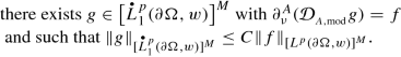
Finally, the fact that u solves the Homogeneous Dirichlet Problem (6.64) formulated for the boundary datum g implies, in light of (6.70)–(6.71) and Theorem 4.12 (with $z=\tfrac {1}{2}$), that u may be uniquely represented as in (6.106) for some constant $c\in {\mathbb {C}}^M$ and some function satisfying (6.107). □

As with the Dirichlet Problem and the Inhomogeneous Regularity Problem (cf. Theorem 6.4 and Theorem 6.6), the solvability results derived in Theorem 6.8 are stable under small perturbations. We leave the formulation of such a result to the interested reader and, instead, prove the following brand of stability result, which does not require flatness for the underlying domain, nor does it explicitly ask for the existence of a distinguished coefficient tensor.

Theorem 6.10

Let $\Omega \subseteq {\mathbb {R}}^{n}$ be an NTA domain with an unbounded Ahlfors regular boundary. Abbreviate $\sigma :={\mathcal {H}}^{n-1}\lfloor \partial \Omega$ and fix an aperture parameter κ > 0. Also, pick some integrability exponent p ∈ (1, ∞) and some Muckenhoupt weight w ∈ A_p(∂ Ω, σ). Finally, consider a homogeneous, second-order, constant complex coefficient, weakly elliptic M × M system L_o in ${\mathbb {R}}^n$ with the property that the Homogeneous Regularity Problem formulated for L_o in Ω as in (6.64) is solvable.

Then there exists an open neighborhood ${\mathcal {U}}$ of L_o in $\mathfrak {L}$ which depends only on n, p, $[w]_{A_p}$, L_o, and the Ahlfors regularity constant of ∂ Ω, with the property that for each system $L\in {\mathcal {U}}$ the Homogeneous Regularity Problem formulated for L in Ω as in (6.64) continues to be solvable.

Proof

For each coefficient tensor $A\in {\mathfrak {A}}_{{ }_{\mathrm {WE}}}$ define the operator

(6.112)

given by

(6.113)

With the piece of notation introduced in (3.13), from (6.113) and (3.143) we see that

(6.114)

is continuous. To proceed, pick an arbitrary $A_o\in {\mathfrak {A}}_{L_o}$. From Proposition 3.6 we see that the solvability of the Homogeneous Regularity Problem formulated for L_o in Ω as in (6.64) is equivalent to having $T_{A_o}$ surjective. Since the set of linear bounded surjective operators between two Banach spaces is open (cf. [70, Lemma 2.4]), we conclude from (6.114) that there exists some small ε > 0 such that T_A in (6.112) is surjective whenever $A\in {\mathfrak {A}}$ satisfies ∥A − A_o∥ < ε. Having established this, another appeal to Proposition 3.6 then proves that there exists an open neighborhood ${\mathcal {U}}$ of L_o in $\mathfrak {L}$, which depends only on n, p, $[w]_{A_p}$, L_o, and the Ahlfors regularity constant of ∂ Ω, with the property that for each system $L\in {\mathcal {U}}$ the Homogeneous Regularity Problem formulated for L in Ω as in (6.64) continues to be solvable. □

6.3 The Neumann Problem in Weighted Lebesgue Spaces

To set the stage, recall the definition of the conormal derivative operator from (3.66).

Theorem 6.11

Let $\Omega \subseteq {\mathbb {R}}^{n}$ be a UR domain. Denote by ν the geometric measure theoretic outward unit normal to Ω, abbreviate $\sigma :={\mathcal {H}}^{n-1}\lfloor \partial \Omega$, and fix an aperture parameter κ > 0. Also, pick an integrability exponent p ∈ (1, ∞) and a Muckenhoupt weight w ∈ A_p(∂ Ω, σ).

Suppose L is a homogeneous, second-order, constant complex coefficient, weakly elliptic M × M system in ${\mathbb {R}}^n$. Select $A\in {\mathfrak {A}}_L$ and consider the Neumann Problem

$$\displaystyle \begin{aligned} \left\lbrace \begin{array}{l} u\in\big[{\mathscr{C}}^{\infty}(\Omega)\big]^M, \\ {} Lu=0\,\,\mathit{\mbox{ in }}\,\,\Omega, \\ {} {\mathcal{N}}_{\kappa}(\nabla u)\in L^p(\partial\Omega,w), \\ {} \partial^A_\nu u=f\in\big[L^p(\partial\Omega,w)\big]^M. \\ {} \end{array} \right. \end{aligned} $$

(6.115)

Then the following statements are valid:

• (a) [ Existence, Estimates, and Integral Representations ] Whenever $A^\top \in {\mathfrak {A}}_{L^{\top }}^{\mathrm {dis}}$ there exists some threshold δ ∈ (0, 1) which depends only on n, p, $[w]_{A_p}$, A, and the Ahlfors regularity constant of ∂ Ω such that if ${\left \lVert \nu \right \rVert }_{[\mathrm {BMO}(\partial \Omega ,\sigma )]^n}<\delta$ ( a scenario which ensures that Ω is a δ-AR domain; cf. Definition 2.15) then $-\tfrac {1}{2}I+K^{\#}_{A^\top }$ is an invertible operator on the Muckenhoupt weighted Lebesgue space [L^p(∂ Ω, w)]^M and the function $u:\Omega \to {\mathbb {C}}^M$ defined as

  $$\displaystyle \begin{aligned} u(x):=\Big({\mathscr{S}}_{{}_{\mathrm{mod}}}\left(-\tfrac{1}{2}I+K^{\#}_{A^\top}\right)^{-1}f\Big)(x) \,\,\mathit{\mbox{ for all }}\,\,x\in\Omega \end{aligned} $$

  (6.116)

  is a solution of the Neumann Problem (6.115) which satisfies

  $$\displaystyle \begin{aligned} {\left\lVert {\mathcal{N}}_{\kappa}(\nabla u) \right\rVert}_{L^p(\partial\Omega,w)}\approx{\left\lVert f \right\rVert}_{[L^p(\partial\Omega,w)]^M}, \end{aligned} $$

  (6.117)

  where the implicit proportionality constants are independent of f. Also, the operator $\partial _\nu ^{A}{\mathcal {D}}_{{ }_{A,\mathrm {mod}}}$ in (4.392) is surjective which implies that, for some constant C ∈ (0, ∞),

  

  (6.118)

  Consequently, the function

  $$\displaystyle \begin{aligned} u:={\mathcal{D}}_{{}_{A,\mathrm{mod}}}g\,\,\mathit{\mbox{ in }}\,\,\Omega \end{aligned} $$

  (6.119)

  is a solution of the Neumann Problem (6.115) which continues to satisfy (6.117).

• (b) [ Additional Integrability ] Under the background assumptions made in item (a), for the solution u of the Neumann Problem (6.115) defined in (6.116), one has the following integrability result: For any given q ∈ (1, ∞) and ω ∈ A_q(∂ Ω, σ), further decreasing δ ∈ (0, 1) ( relative to q and $[\omega ]_{A_q}$) one has

  $$\displaystyle \begin{aligned} {\mathcal{N}}_{\kappa}(\nabla u)\in L^q(\partial\Omega,\omega)\Longleftrightarrow f\in\big[L^q(\partial\Omega,\omega)\big]^M \end{aligned} $$

  (6.120)

  and if either of these conditions holds then

  $$\displaystyle \begin{aligned} {\left\lVert {\mathcal{N}}_{\kappa}(\nabla u) \right\rVert}_{L^q(\partial\Omega,\omega)} \approx{\left\lVert f \right\rVert}_{[L^q(\partial\Omega,\omega)]^M}. \end{aligned} $$

  (6.121)

• (c) [ Uniqueness (modulo constants) ] Assume $A\in {\mathfrak {A}}_{L}^{\mathrm {dis}}$. Then there exists δ ∈ (0, 1) which depends only on n, p, $[w]_{A_p}$, A, and the Ahlfors regularity constant of ∂ Ω such that whenever ${\left \lVert \nu \right \rVert }_{[\mathrm {BMO}(\partial \Omega ,\sigma )]^n}<\delta$ ( hence, whenever Ω is a δ-AR domain; cf. Definition 2.15) it follows that any two solutions of the Neumann Problem (6.115) differ by a constant from ${\mathbb {C}}^M$.

• (d) [ Well-Posedness ] Whenever $A\in {\mathfrak {A}}_{L}^{\mathrm {dis}}$ and $A^\top \in {\mathfrak {A}}_{L^\top }^{\mathrm {dis}}$ there exists δ ∈ (0, 1) which depends only on n, p, $[w]_{A_p}$, A, and the Ahlfors regularity constant of ∂ Ω such that if ${\left \lVert \nu \right \rVert }_{[\mathrm {BMO}(\partial \Omega ,\sigma )]^n}<\delta$ ( i.e., if Ω is a δ-AR domain; cf. Definition 2.15) then the Neumann Problem (6.115) is solvable, the solution is unique modulo constants from ${\mathbb {C}}^M$, and each solution satisfies (6.117).

• (e) [ Sharpness ] If $A^\top \notin {\mathfrak {A}}_{L^{\top }}^{\mathrm {dis}}$ then the Neumann Problem (6.115) may not be solvable. In addition, if $A\notin {\mathfrak {A}}_{L}^{\mathrm {dis}}$ then the Neumann Problem (6.115) may have more than one solution. In fact, even the two-dimensional Laplacian may be written as Δ = div A∇ for some matrix $A\in {\mathbb {C}}^{2\times 2}$ ( not belonging to ${\mathfrak {A}}_{\Delta }^{\mathrm {dis}}=\{I_{2\times 2}\}$) such that the Neumann Problem formulated for this as in (6.115) for this choice of A and with $\Omega :={\mathbb {R}}^2_{+}$ fails to have a solution for each non-zero boundary datum belonging to an infinite dimensional linear subspace of L^p(∂ Ω, w), and the linear space of null-solutions for the Neumann Problem formulated as in (6.115) for this choice of A and with $\Omega :={\mathbb {R}}^2_{+}$ is actually infinite dimensional.

Remark 6.6

In view of (2.576), (3.66), and the Fatou-type result described in Theorem 3.4 it follows that the conormal derivative $\partial ^A_\nu u$ is well defined in the context of (6.115).

Remark 6.7

In special circumstances, the statement of Theorem 6.11 may be further streamlined. For example, Theorem 3.8 gives that if the system L actually satisfies the strong Legendre–Hadamard ellipticity condition then for the well-posedness formulated in item (d) it suffices to assume that $A\in {\mathfrak {A}}_{L}^{\mathrm {dis}}$, and if n ≥ 3, M = 1, it suffices to assume that the matrix $A\in {\mathfrak {A}}_L$ is symmetric.

Remark 6.8

The solvability result presented in Theorem 6.11 is relevant in relation to the issue singled out as Question 2.5 in [137].

We now turn to the task of presenting the proof of Theorem 6.11.

Proof of Theorem 6.11

Assume first that the coefficient tensor $A\in {\mathfrak {A}}_L$ is such that $A^\top \in {\mathfrak {A}}_{L^{\top }}^{\mathrm {dis}}$. From the current assumptions and Theorem 4.8 we know that there exists some threshold δ ∈ (0, 1), whose nature is as specified in the statement of the theorem, such that if ${\left \lVert \nu \right \rVert }_{[\mathrm {BMO}(\partial \Omega ,\sigma )]^n}<\delta$ then the operator $-\tfrac {1}{2}I+K^{\#}_{A^\top }$ is invertible on [L^p(∂ Ω, w)]^M. Granted this, item (c) in Proposition 3.5 then guarantees that the function (6.116) solves the Neumann Problem (6.115) and satisfies (6.117).

Next, the claims in (6.118) are consequences of the surjectivity of the operator (4.392) (itself implied by item (2) of Theorem 4.13), and the Open Mapping Theorem. In turn, (6.118) and Theorem 3.5 guarantee that the function u in (6.119) solves the Neumann Problem (6.115) and satisfies (6.117). This takes care of the claims in item (a).

Let us now turn our attention to the claim made in item (b), concerning additional integrability properties for the solution constructed in (6.116). The right-pointing implication in (6.120) together with the right-pointing inequality in (6.121) are simple consequences of the fact that we have $|f|=\big |\partial ^A_\nu u\big |\leq C{\mathcal {N}}_{\kappa }(\nabla u)$ at σ-a.e. point on ∂ Ω. The left-pointing implication in (6.120) along with the left-pointing inequality in (6.121) are seen from (6.116), (4.342), and Proposition 3.5.

To prove uniqueness modulo constants in the case when $A\in {\mathfrak {A}}_{L}^{\mathrm {dis}}$, suppose u solves the homogeneous version of the Neumann Problem (6.115) (corresponding to f = 0). Also, fix two arbitrary indices ℓ ∈{1, …, n} and γ ∈{1, …, M}. Since by (3.66) the second integral in (6.62) involves $\nu _ra_{rs}^{\alpha \beta }(\partial _s u_\beta )\big |{ }^{{ }^{\kappa -\mathrm {n.t.}}}_{\partial \Omega } =\big (\partial ^A_\nu u\big )_\alpha =0$ for each α ∈{1, …, M}, we conclude that we presently have

$$\displaystyle \begin{aligned} (\partial_\ell u_\gamma)(x) &=\int_{\partial\Omega} a^{\beta\alpha}_{rs}(\partial_r E_{\gamma\beta})(x-y)\Big\{ \nu_\ell(y)\big((\partial_s u_\alpha)\big|{}_{\partial\Omega}^{{}^{\kappa-\mathrm{n.t.}}}\big)(y) \\ {} &\hskip 1.60in -\nu_s(y)\big((\partial_\ell u_\alpha)\big|{}_{\partial\Omega}^{{}^{\kappa-\mathrm{n.t.}}}\big)(y)\Big\}\,\mbox{d}\sigma(y) \end{aligned} $$

(6.122)

at every point x ∈ Ω. On account of (3.86), going nontangentially to the boundary in (6.122) then yields

(6.123)

at σ-a.e. x ∈ ∂ Ω. For each r ∈{1, …, n} and β ∈{1, …, M} we may rely on (3.17) to write

$$\displaystyle \begin{aligned} \widehat{\partial_r E_{\gamma\beta}}\big(\nu(x)\big) =\mbox{i}\nu_r(x)\widehat{E_{\gamma\beta}}\big(\nu(x)\big) =\mbox{i}\nu_r(x)\big[L\big(\nu(x)\big)\big]^{-1}_{\gamma\beta} \end{aligned} $$

(6.124)

at σ-a.e. x ∈ ∂ Ω. For ease of notation, henceforth we agree to abbreviate

$$\displaystyle \begin{aligned} \begin{array}{c} \big(\partial_{\,T_{jk}}u_\alpha\big)(x):=\nu_j(x)\big((\partial_k u_\alpha)\big|{}_{\partial\Omega}^{{}^{\kappa-\mathrm{n.t.}}}\big)(x) -\nu_k(x)\big((\partial_j u_\alpha)\big|{}_{\partial\Omega}^{{}^{\kappa-\mathrm{n.t.}}}\big)(x) \\ {} \mbox{for each }{j,k\in\{1,\dots,n\}}, {\alpha\in\{1,\dots,M\}},\mbox{ and }{\sigma}\mbox{-a.e. }{x\in\partial\Omega}. \end{array} \end{aligned} $$

(6.125)

Bring in an additional index t ∈{1, …, n}. If we now multiply (6.123) by ν_t(x) then subtract from the resulting formula its version with ℓ and t interchanged we then arrive, bearing in mind (6.124), (6.125), (3.2), at the identity

(6.126)

valid for each t, ℓ ∈{1, …, n}, each γ ∈{1, …, M}, and σ-a.e. x ∈ ∂ Ω. In relation to (6.126), we make several observations. For starters, the first line in the right-hand side of (6.126) is

$$\displaystyle \begin{aligned} \frac{1}{2}\big[L\big(\nu(x)\big)\big]_{\beta\alpha} & \big[L\big(\nu(x)\big)\big]^{-1}_{\gamma\beta}\big(\partial_{\,T_{t\ell}}u_\alpha\big)(x) \\ {} &=\frac{1}{2}\delta_{\gamma\alpha}\big(\partial_{\,T_{t\ell}}u_\alpha\big)(x) =\frac{1}{2}\big(\partial_{\,T_{t\ell}}u_\gamma\big)(x). \end{aligned} $$

(6.127)

This may be absorbed in the left-hand side of (6.126), which subsequently becomes $\frac {1}{2}\big (\partial _{\,T_{t\ell }}u_\gamma \big )(x)$. The second observation is that, as is visible from (3.24), the second line in the right-hand side of (6.126) is precisely

$$\displaystyle \begin{aligned} \Big(K_{A}\big(\partial_{\,T_{t\ell}}u\big)\Big)_\gamma(x),\,\,\mbox{ where }\,\, \partial_{\,T_{t\ell}}u:=\big(\partial_{\,T_{t\ell}}u_\alpha\big)_{1\leq\alpha\leq M}. \end{aligned} $$

(6.128)

The final observation we wish to make with regard to (6.126) is that the third and fourth lines in the right-hand side of (6.126) are commutators of the form

$$\displaystyle \begin{aligned} \Big(\big[M_{\nu},T\big]\big(\partial_T u\big)\Big)(x). \end{aligned} $$

(6.129)

Above, M_ν denotes the operator of pointwise multiplication by generic scalar components of ν. Also, T stands for the principal-value singular integral operator of formal convolution type with a suitable matrix-valued kernel whose entries are linear combinations with coefficients which are entries from A of generic first-order partial derivatives of generic entries of the matrix E. Finally, ∂_Tu stands for generic functions of the form $\partial _{\,T_{t\ell }}u_\alpha$ with 1 ≤ ℓ, t ≤ n and 1 ≤ α ≤ M.

In view of these observations, we may recast (6.126) as

$$\displaystyle \begin{aligned} \begin{array}{c} \frac{1}{2}\partial_{\,T_{t\ell}}u=K_{A}\big(\partial_{\,T_{t\ell}}u\big) +\big[M_{\nu},T\big]\big(\partial_Tu\big) \\ {} \mbox{at }{\sigma}\mbox{-a.e. point on }{\partial\Omega}\mbox{, for each }{t,\ell\in\{1,\dots,n\}}. \end{array} \end{aligned} $$

(6.130)

Since we are currently assuming that $A\in {\mathfrak {A}}_{L}^{\mathrm {dis}}$, from (6.130), (4.299), and Theorem 4.3 (whose applicability in the present context takes into account the format of T specified above as well as Proposition 3.4) we then conclude that for each t, ℓ ∈{1, …, n} we have

$$\displaystyle \begin{aligned} \frac{1}{2}\big\|\partial_{\,T_{t\ell}}u\big\|{}_{[L^p(\partial\Omega,w)]^M} &\leq C_\delta\big\|\partial_{\,T_{t\ell}}u\big\|{}_{[L^p(\partial\Omega,w)]^M} +C_\delta\sum_{j,k=1}^n\big\|\partial_{\,T_{jk}}u\big\|{}_{[L^p(\partial\Omega,w)]^M} \\ {} &\mbox{where }{C_\delta=o(1)}\mbox{ as }{\delta\to 0^{+}}. \end{aligned} $$

(6.131)

After summing up in all t, ℓ ∈{1, …, n} we conclude from (6.131) that

$$\displaystyle \begin{aligned} \frac{1}{2}\sum_{t,\ell=1}^n\big\|\partial_{\,T_{t\ell}}u\big\|{}_{[L^p(\partial\Omega,w)]^M} &\leq C_\delta\sum_{t,\ell=1}^n\big\|\partial_{\,T_{t\ell}}u\big\|{}_{[L^p(\partial\Omega,w)]^M} \\ {} &\quad \mbox{with }{C_\delta=o(1)}\mbox{ as }{\delta\to 0^{+}}. \end{aligned} $$

(6.132)

Assuming δ ∈ (0, 1) is sufficiently small to begin with, it follows from (6.132) that

$$\displaystyle \begin{aligned} \sum_{t,\ell=1}^n\big\|\partial_{\,T_{t\ell}}u\big\|{}_{[L^p(\partial\Omega,w)]^M}\leq 0 \end{aligned} $$

(6.133)

hence, necessarily,

$$\displaystyle \begin{aligned} \partial_{\,T_{t\ell}}u_\alpha=0\,\,\mbox{ for each }\,\,t,\ell\in\{1,\dots,n\}\,\,\mbox{ and }\,\,\alpha\in\{1,\dots,M\}. \end{aligned} $$

(6.134)

In concert with (6.125) and (6.122) this ultimately shows that

$$\displaystyle \begin{aligned} \partial_\ell u_\gamma=0\,\,\mbox{ in }\,\,\Omega\,\,\mbox{ for each }\,\,\ell\in\{1,\dots,n\} \,\,\mbox{ and }\,\,\gamma\in\{1,\dots,M\}. \end{aligned} $$

(6.135)

Thus, the function u is locally constant in Ω. Since the latter is a connected set (cf. Theorem 2.4), we conclude that there exists a constant $c\in {\mathbb {C}}^M$ such that u ≡ c in Ω.

An alternative proof of uniqueness modulo constants in the case when $A\in {\mathfrak {A}}_{L}^{\mathrm {dis}}$ goes as follows. Suppose $u\in \big [{\mathscr {C}}^{\infty }(\Omega )\big ]^M$ is a function satisfying Lu = 0 in Ω, as well as ${\mathcal {N}}_{\kappa }(\nabla u)\in L^p(\partial \Omega ,w)$, and $\partial ^A_\nu u=0$. Then Corollary 3.1 implies that $g:=u\big |{ }^{{ }^{\kappa -\mathrm {n.t.}}}_{\partial \Omega }$ exists σ-a.e. on ∂ Ω, belongs to , and

$$\displaystyle \begin{aligned} u={\mathcal{D}}_{{}_{A,\mathrm{mod}}}g+c\,\,\mbox{ in }\,\,\Omega, \end{aligned} $$

(6.136)

for some constant $c\in {\mathbb {C}}^M$ (recall that the present assumptions ensure that Ω is a connected set; cf. Theorem 2.4). In light of the jump-formula (3.134), going nontangentially to the boundary in (6.136) then yields $\big (-\tfrac {1}{2}I+K_{{ }_{A,\mathrm {mod}}}\big )g=-c$, hence

(6.137)

Since we are currently assuming that $A\in {\mathfrak {A}}_{L}^{\mathrm {dis}}$, from this and Theorem 4.12 (with $z=-\tfrac {1}{2}$) we conclude that , i.e., g is a constant on ∂ Ω. Having established this, from (6.136) and (3.54) we then conclude that u is a constant in Ω, as wanted.

Next, the claims in (d) are direct consequences of results established in items (a) and (c). As regards the claims made in item (e), consider the Laplacian Δ in ${\mathbb {R}}^2\equiv {\mathbb {C}}$, written as Δ = a_jk∂_j∂_k, where the coefficient tensor A = (a_jk)_1≤j,k≤2 is the 2 × 2 complex matrix

$$\displaystyle \begin{aligned} A:=\begin{pmatrix} 1 & -\mbox{i} \\ \mbox{i} & 1 \end{pmatrix}. \end{aligned} $$

(6.138)

Fix an aperture parameter κ ∈ (0, ∞), an integrability exponent p ∈ (1, ∞), and a Muckenhoupt weight $w\in A_p({\mathbb {R}},{\mathcal {L}}^1)$. We claim that the space of admissible boundary data for the L^p-Neumann boundary value problem for the Laplacian in the upper-half plane where the prescribed conormal derivative is the one associated with the matrix A may be described as

$$\displaystyle \begin{aligned} \Big\{\partial_\nu^A u &:\,u\in{\mathscr{C}}^{\infty}({\mathbb{R}}^2_{+}),\,\, \Delta u=0\,\,\mbox{ in }\,\,{\mathbb{R}}^2_{+},\,\,{\mathcal{N}}_{\kappa}(\nabla u)\in L^p({\mathbb{R}},w)\Big\} \\ {} &\qquad =\Big\{f\in L^p({\mathbb{R}},w):\,Hf=-\mbox{i}f\Big\}, \end{aligned} $$

(6.139)

where H is the Hilbert transform on the real line (cf. (1.24)). Given that the latter space has infinite codimension in $L^p({\mathbb {R}},w)$ (since H² = −I on this space), the identification in (6.139) suits our present purposes.

To prove the left-to-right inclusion in (6.139), pick a complex-valued function u satisfying

$$\displaystyle \begin{aligned} u\in{\mathscr{C}}^{\infty}({\mathbb{R}}^2_{+}),\quad \Delta u=0\,\,\mbox{ in }\,\,{\mathbb{R}}^2_{+},\quad {\mathcal{N}}_{\kappa}(\nabla u)\in L^p({\mathbb{R}},w). \end{aligned} $$

(6.140)

On account of the Fatou-type result recalled in Theorem 3.4, these properties guarantee that $(\nabla u)\big |{ }^{{ }^{\kappa -\mathrm {n.t.}}}_{\partial {\mathbb {R}}^2_{+}}$ exists at ${\mathcal {L}}^1$-a.e. point on $\partial {\mathbb {R}}^2_{+}$. In particular, $f:=\partial ^A_\nu u$ is a well-defined function in $L^p({\mathbb {R}},w)$. More specifically, bearing in mind that the outward unit normal for the upper-half plane is ν = (ν₁, ν₂) = (0, −1) ≡−i, from (3.66) we see that

$$\displaystyle \begin{aligned} f &=\partial^A_\nu u=\nu_ra_{rs}\big(\partial_s u\big)\big|{}^{{}^{\kappa-\mathrm{n.t.}}}_{\partial{\mathbb{R}}^2_{+}} \\ {} &=\nu_1\big(\partial_1 u\big)\big|{}^{{}^{\kappa-\mathrm{n.t.}}}_{\partial{\mathbb{R}}^2_{+}} -\mbox{i}\nu_1\big(\partial_2 u\big)\big|{}^{{}^{\kappa-\mathrm{n.t.}}}_{\partial{\mathbb{R}}^2_{+}} +\mbox{i}\nu_2\big(\partial_1 u\big)\big|{}^{{}^{\kappa-\mathrm{n.t.}}}_{\partial{\mathbb{R}}^2_{+}} +\nu_2\big(\partial_2 u\big)\big|{}^{{}^{\kappa-\mathrm{n.t.}}}_{\partial{\mathbb{R}}^2_{+}} \\ {} &=(\nu_1+\mbox{i}\nu_2)\Big((\partial_1 u)\big|{}^{{}^{\kappa-\mathrm{n.t.}}}_{\partial{\mathbb{R}}^2_{+}} -\mbox{i}(\partial_2 u)\big|{}^{{}^{\kappa-\mathrm{n.t.}}}_{\partial{\mathbb{R}}^2_{+}}\Big) =2\nu(\partial_{z}u)\big|{}^{{}^{\kappa-\mathrm{n.t.}}}_{\partial{\mathbb{R}}^2_{+}} \\ {} &=-2\mbox{i}(\partial_{z}u)\big|{}^{{}^{\kappa-\mathrm{n.t.}}}_{\partial{\mathbb{R}}^2_{+}} \,\,\mbox{ at }{{\mathcal{L}}^1}\mbox{-a.e. point on }\,\,\partial{\mathbb{R}}^2_{+}\equiv{\mathbb{R}}, \end{aligned} $$

(6.141)

where $\partial _{z}:=\tfrac {1}{2}(\partial _{x}-\mbox{i}\partial _{y})$ is the complex conjugate of the Cauchy–Riemann operator $\partial _{\bar {z}}:=\tfrac {1}{2}(\partial _{x}+\mbox{i}\partial _{y})$. Hence, if we define

$$\displaystyle \begin{aligned} U:=2\partial_{z}u\,\,\mbox{ in }\,\,{\mathbb{R}}^2_{+}, \end{aligned} $$

(6.142)

upon recalling that $\Delta =4\partial _{\bar {z}}\partial _{z}$, the properties in (6.140) imply

$$\displaystyle \begin{aligned} U\in{\mathscr{C}}^{\infty}({\mathbb{R}}^2_{+}),\quad \partial_{\bar{z}}w=0\,\,\mbox{ in }\,\,{\mathbb{R}}^2_{+},\quad {\mathcal{N}}_{\kappa}w\in L^p({\mathbb{R}},w). \end{aligned} $$

(6.143)

These simply amount to stating that U is a holomorphic function belonging to the Muckenhoupt weighted Hardy space ${\mathcal {H}}^p({\mathbb {R}}^2_{+},w)$ associated with the Cauchy–Riemann operator in the upper-half plane. In addition, (6.141) tells us that

$$\displaystyle \begin{aligned} U\big|{}^{{}^{\kappa-\mathrm{n.t.}}}_{\partial{\mathbb{R}}^2_{+}}=\mbox{i}f \,\,\mbox{ at }{{\mathcal{L}}^1}\mbox{-a.e. point on }\,\,\partial{\mathbb{R}}^2_{+}\equiv{\mathbb{R}}. \end{aligned} $$

(6.144)

Together with Cauchy’s reproducing formula for holomorphic functions in the aforementioned Hardy space, this gives

$$\displaystyle \begin{aligned} U(z)=\frac{1}{2\pi}\int_{\mathbb{R}}\frac{f(t)}{t-z}\,\mbox{d}t\,\,\mbox{ for each }\,\,z\in{\mathbb{C}}_{+}. \end{aligned} $$

(6.145)

After taking the nontangential trace to the boundary in (6.145) we arrive at the conclusion that $\mbox{i}f=\mbox{i}\big (\tfrac {1}{2}I+-\frac {1}{2\mbox{i}}H\big )f$ at ${\mathcal {L}}^1$-a.e. point in ${\mathbb {R}}$. This ultimately proves that f must satisfy the compatibility condition

$$\displaystyle \begin{aligned} Hf=-\mbox{i}f\,\,\mbox{ at }{{\mathcal{L}}^1}\mbox{-a.e. point in }\,\,{\mathbb{R}}. \end{aligned} $$

(6.146)

The left-to-right inclusion in (6.139) is therefore established.

To justify the converse inclusion, consider $f\in L^p({\mathbb {R}},w)$ satisfying Hf = −if at ${\mathcal {L}}^1$-a.e. point in ${\mathbb {R}}$. Bring ${\mathscr {S}}_{{ }_{\mathrm {mod}}}$, the modified boundary-to-domain harmonic single layer potential operator associated with the Laplacian in the upper-half plane (cf. (3.38)), and note that

$$\displaystyle \begin{aligned} 2\mbox{i}\partial_{z}({\mathscr{S}}_{{}_{\mathrm{mod}}}f)(z) =\frac{1}{2\pi\mbox{i}}\int_{\mathbb{R}}\frac{f(t)}{t-z}\,\mbox{d}t\,\,\mbox{ for each }\,\,z\in{\mathbb{C}}_{+}. \end{aligned} $$

(6.147)

If we define $u:={\mathscr {S}}_{{ }_{\mathrm {mod}}}f$ in ${\mathbb {R}}^2_{+}$, then this function belongs to ${\mathscr {C}}^{\infty }({\mathbb {R}}^2_{+})$, satisfies Δu = 0 in ${\mathbb {R}}^2_{+}$, has ${\mathcal {N}}_{\kappa }(\nabla u)\in L^p({\mathbb {R}},w)$, and (6.147) permits us to compute

$$\displaystyle \begin{aligned} \partial_\nu^A u &=2\mbox{i}\big(\partial_{z}u\big)\big|{}^{{}^{\kappa-\mathrm{n.t.}}}_{\partial{\mathbb{R}}^2_{+}} =2\mbox{i}(\partial_{z}{\mathscr{S}}_{{}_{\mathrm{mod}}}f)\big|{}^{{}^{\kappa-\mathrm{n.t.}}}_{\partial{\mathbb{R}}^2_{+}} \\ {} &=\tfrac{1}{2}f-\tfrac{1}{2\mbox{i}}Hf=\tfrac{1}{2}f+\tfrac{1}{2}f=f, \end{aligned} $$

(6.148)

as wanted.

As regards the space of null-solutions for the L^p-Neumann Problem (6.115) in the case when n = 2, M = 1, L =  Δ (the two-dimensional Laplacian), $\Omega ={\mathbb {R}}^2_{+}$, and A as in (6.138), we claim that

$$\displaystyle \begin{aligned} \Big\{u\in{\mathscr{C}}^{\infty}&({\mathbb{R}}^2_{+}):\,\, \Delta u=0\,\,\mbox{ in }\,\,{\mathbb{R}}^2_{+},\,\,{\mathcal{N}}_{\kappa}(\nabla u)\in L^p({\mathbb{R}},w), \,\,\partial_\nu^A u=0\Big\} \\ {} &\qquad =\Big\{\overline{U}:\,{U}\mbox{ holomorphic in }{{{\mathbb{R}}^2_{+}}},\mbox{ with }\,\, {\mathcal{N}}_{\kappa}(\nabla U)\in L^p({\mathbb{R}},w)\Big\}. \end{aligned} $$

(6.149)

To justify this identification, pick an arbitrary function belonging to the space in the left side of (6.149). Then ∂_zu is holomorphic in ${\mathbb {R}}^2_{+}$ (since $\partial _{\bar {z}}\partial _{z}=\tfrac {1}{4}\Delta$), and satisfies ${\mathcal {N}}_{\kappa }(\partial _{z}u)\in L^p({\mathbb {R}},w)$. As such, ∂_zu belongs to ${\mathcal {H}}^p({\mathbb {R}}^2_{+},w)$, the Muckenhoupt weighted Hardy space in the upper-half plane for the Cauchy–Riemann operator. Since from (6.141) we have

$$\displaystyle \begin{aligned} (\partial_{z}u)\big|{}^{{}^{\kappa-\mathrm{n.t.}}}_{\partial{\mathbb{R}}^2_{+}}=0 \,\,\mbox{ at }{{\mathcal{L}}^1}\mbox{-a.e. point on }\,\,\partial{\mathbb{R}}^2_{+}\equiv{\mathbb{R}}, \end{aligned} $$

(6.150)

we may rely on Cauchy’s reproducing formula to conclude that ∂_zu vanishes identically in ${\mathbb {R}}^2_{+}$. Hence, $U:=\overline {u}$ is a holomorphic function in ${\mathbb {R}}^2_{+}$. This places $\overline {U}$ (and, ultimately, u) in the space in the right side of (6.149). In the opposite direction, given any holomorphic function U in ${\mathbb {R}}^2_{+}$ satisfying ${\mathcal {N}}_{\kappa }(\nabla U)\in L^p({\mathbb {R}},w)$, the function $u:=\overline {U}$ is harmonic in ${\mathbb {R}}^2_{+}$, has ${\mathcal {N}}_{\kappa }(\nabla u)\in L^p({\mathbb {R}},w)$ and, much as in (6.141), we see that

$$\displaystyle \begin{aligned} \partial^A_\nu u &=-2\mbox{i}(\partial_{z}u)\big|{}^{{}^{\kappa-\mathrm{n.t.}}}_{\partial{\mathbb{R}}^2_{+}} =-2\mbox{i}\overline{(\partial_{\bar{z}}\overline{u})\big|{}^{{}^{\kappa-\mathrm{n.t.}}}_{\partial{\mathbb{R}}^2_{+}}} \\ {} &=-2\mbox{i}\overline{(\partial_{\bar{z}}U)\big|{}^{{}^{\kappa-\mathrm{n.t.}}}_{\partial{\mathbb{R}}^2_{+}}} =0\,\,\mbox{ at }{{\mathcal{L}}^1}\mbox{-a.e. point on }\,\,\partial{\mathbb{R}}^2_{+}\equiv{\mathbb{R}}, \end{aligned} $$

(6.151)

given that U is holomorphic in ${\mathbb {R}}^2_{+}\equiv {\mathbb {C}}_{+}$. This completes the proof of (6.149). The space in the right side of (6.149) is infinite dimensional since, for example, for each $m\in {\mathbb {N}}$ the function ${\mathbb {C}}_{+}\ni z\mapsto (\bar {z}-\mbox{i})^{-m}\in {\mathbb {C}}$ belongs to this space. We therefore conclude that the space of null-solutions for the L^p-Neumann Problem (6.115) is, as claimed, infinite dimensional. □

Remark 6.9

For similar reasons as in past situations, a solvability result which is analogous to the one described in Theorem 6.11 also holds for the Neumann Problem with data in Lorentz spaces, i.e., for

$$\displaystyle \begin{aligned} \left\lbrace \begin{array}{l} u\in\big[{\mathscr{C}}^{\infty}(\Omega)\big]^M, \\ {} Lu=0\,\,\mbox{ in }\,\,\Omega, \\ {} {\mathcal{N}}_{\kappa}(\nabla u)\in L^{p,q}(\partial\Omega,\sigma), \\ {} \partial^A_\nu u=f\in\big[L^{p,q}(\partial\Omega,\sigma)\big]^M, \\ {} \end{array} \right. \end{aligned} $$

(6.152)

with p ∈ (1, ∞) and q ∈ (0, ∞].

See Theorem 8.21 (and also Examples 8.2, 8.6) for more general results of this flavor.

Remark 6.10

In light of the remarks made in (3.228)–(3.229), Theorem 6.11 applies in the case of the Lamé system L_μ,λ = μ Δ + (λ + μ)∇div in ${\mathbb {R}}^n$ with n ≥ 2, assuming μ ≠ 0, 2μ + λ ≠ 0, and 3μ + λ ≠ 0. Specifically, if $\Omega \subseteq {\mathbb {R}}^n$ is a δ-AR domain, and w ∈ A_p(∂ Ω, σ) with p ∈ (1, ∞), then if δ ∈ (0, 1) sufficiently small (relative to μ, λ, p, $[w]_{A_p}$, and the Ahlfors regularity constant of ∂ Ω) the Neumann Problem (6.115), which in this case reads

$$\displaystyle \begin{aligned} \left\lbrace \begin{array}{l} u\in\big[{\mathscr{C}}^{\infty}(\Omega)\big]^n, \\ {} \mu\Delta u+(\lambda+\mu)\nabla\mathrm{div}u=0\,\,\mbox{ in }\,\,\Omega, \\ {} {\mathcal{N}}_{\kappa}(\nabla u)\in L^p(\partial\Omega,w), \\ {} \partial^{A(\zeta)}_\nu u=\Big[\mu(\nabla u)^\top+\zeta(\nabla u)\Big]\Big|{}^{{}^{\kappa-\mathrm{n.t.}}}_{\partial\Omega}\nu +(\mu+\lambda-\zeta)(\mathrm{div}u)\big|{}^{{}^{\kappa-\mathrm{n.t.}}}_{\partial\Omega}\nu=f \\ {} \end{array} \right. \end{aligned} $$

(6.153)

is solvable (in the explicit manner described in (6.116)) for each given function f ∈[L^p(∂ Ω, w)]ⁿ, provided the coefficient tensor A(ζ) is as in (3.226) with

$$\displaystyle \begin{aligned} \zeta:=\frac{\mu(\mu+\lambda)}{3\mu+\lambda}. \end{aligned} $$

(6.154)

Moreover, the solution is unique modulo constants from ${\mathbb {C}}^n$ and each solution satisfies (6.117) (with M := n).

By way of contrast, in the two-dimensional case, Corollary 4.3 ensures that the Neumann Problem (6.153) is actually solvable (again, in the manner described in (6.116), the solution being unique modulo constants from ${\mathbb {C}}^2$ and each solution satisfying a naturally accompanying estimate) for each given function f in the space [L^p(∂ Ω, w)]², in the larger range

$$\displaystyle \begin{aligned} \zeta\in{\mathbb{C}}\setminus\Big\{-\mu,\tfrac{\mu(5\mu+3\lambda)}{3\mu+\lambda}\Big\}. \end{aligned} $$

(6.155)

In particular, if we also demand that μ + λ ≠ 0 then ζ := μ becomes an admissible value, as far as (6.155) is concerned, and from (4.438), (6.116) we see that the Neumann Problem (6.153) with ζ := μ is solvable uniquely (modulo constants) for each given function f ∈[L^p(∂ Ω, w)]². This is of interest since said problem involves the so-called traction conormal derivative, i.e.,

$$\displaystyle \begin{aligned} \partial^{A(\mu)}_\nu u=\mu\Big[(\nabla u)^\top+(\nabla u)\Big]\Big|{}^{{}^{\kappa-\mathrm{n.t.}}}_{\partial\Omega}\nu +\lambda(\mathrm{div}u)\big|{}^{{}^{\kappa-\mathrm{n.t.}}}_{\partial\Omega}\nu, \end{aligned} $$

(6.156)

which is particularly relevant in physics and engineering.

It is also of interest to note that the solvability result from Theorem 6.11 is stable under small perturbations. Specifically, by reasoning similarly as in the proof of Theorem 6.4 (while also bearing in mind Theorem 3.9) yields the following theorem.

Theorem 6.12

Retain the original background assumptions on the set Ω from Theorem 6.11 and, as before, fix an integrability exponent p ∈ (1, ∞) along with a Muckenhoupt weight w ∈ A_p(∂ Ω, σ). Then the following statements are true.

• (a) [ Existence ] Given any system $L_o\in \mathfrak {L}$ with $L_o^\top \in \mathfrak {L}^{\mathrm {dis}}$ ( cf. (3.195)) , it follows that for each $A_o\in \mathfrak {A}_{L_o}$ with $A_o^\top \in \mathfrak {A}^{\mathrm {dis}}_{L_o^\top }$ there exist a threshold δ ∈ (0, 1) and an open neighborhood ${\mathcal {U}}$ of A_o in $\mathfrak {A}$, both of which depend only on n, p, $[w]_{A_p}$, A_o, and the Ahlfors regularity constant of ∂ Ω, with the property that if ${\left \lVert \nu \right \rVert }_{[\mathrm {BMO}(\partial \Omega ,\sigma )]^n}<\delta$ (i.e., if Ω is a δ-AR domain) then for each coefficient tensor $A\in {\mathcal {U}}$ the Neumann Problem (6.115) formulated for the system L_A ( cf. (3.7)) and the conormal derivative associated with A ( cf. (3.66)) is actually solvable.

• (b) [ Uniqueness ] Assume $L_o\in \mathfrak {L}^{\mathrm {dis}}$ and fix some $A_o\in \mathfrak {A}^{\mathrm {dis}}_{L_o}$. Then there exist a threshold δ ∈ (0, 1) and an open neighborhood ${\mathcal {U}}$ of A_o in $\mathfrak {A}$, both of which depend only on n, p, $[w]_{A_p}$, L_o, and the Ahlfors regularity constant of ∂ Ω, with the following significance: Whenever ${\left \lVert \nu \right \rVert }_{[\mathrm {BMO}(\partial \Omega ,\sigma )]^n}<\delta$ ( i.e., Ω is a δ-AR domain) then for each coefficient tensor $A\in {\mathcal {U}}$ it follows that any two solutions of the Neumann Problem (6.115) formulated for the system L_A ( cf. (3.7)) and the conormal derivative associated with A ( cf. (3.66)) differ by a constant in ${\mathbb {C}}^M$.

• (c) [ Well-Posedness ] Assuming $L_o\in \mathfrak {L}^{\mathrm {dis}}$ and $L_o^\top \in \mathfrak {L}^{\mathrm {dis}}$, fix some $A_o\in \mathfrak {A}^{\mathrm {dis}}_{L_o}$. Then there exist a threshold δ ∈ (0, 1) and an open neighborhood ${\mathcal {U}}$ of A_o in $\mathfrak {A}$, both of which depend only on n, p, $[w]_{A_p}$, L_o, and the Ahlfors regularity constant of ∂ Ω, with the following significance: Whenever ${\left \lVert \nu \right \rVert }_{[\mathrm {BMO}(\partial \Omega ,\sigma )]^n}<\delta$ ( i.e., Ω is a δ-AR domain) then for each coefficient tensor $A\in {\mathcal {U}}$ it follows that any two solutions of the Neumann Problem (6.115) formulated for the system L_A ( cf. (3.7)) and the conormal derivative associated with A ( cf. (3.66)) is solvable, and any two solutions differ by a constant from ${\mathbb {C}}^M$.

In addition to Theorem 6.12, there is yet another type of stability result for the Neumann problem which does not require flatness for the underlying domain, nor does it explicitly ask for the existence of a distinguished coefficient tensor (compare with Theorem 6.10).

Theorem 6.13

Let $\Omega \subseteq {\mathbb {R}}^{n}$ be an NTA domain with an unbounded Ahlfors regular boundary. Abbreviate $\sigma :={\mathcal {H}}^{n-1}\lfloor \partial \Omega$ and denote by ν the geometric measure theoretic outward unit normal to Ω. Also, fix an aperture parameter κ > 0, pick an integrability exponent p ∈ (1, ∞), and choose some arbitrary Muckenhoupt weight w ∈ A_p(∂ Ω, σ). Finally, consider a coefficient tensor $A_o\in {\mathfrak {A}}_{{ }_{\mathrm {WE}}}$ with the property that the Neumann Problem formulated for the system $L:=L_{A_o}$ ( cf. (3.7)) and the conormal derivative associated with A_o ( cf. (3.66)) as in (6.115) is solvable.

Then there exists an open neighborhood ${\mathcal {U}}$ of A_o in $\mathfrak {A}$ which depends only on n, p, $[w]_{A_p}$, A_o, and the Ahlfors regularity constant of ∂ Ω, with the property that for each coefficient tensor $A\in {\mathcal {U}}$ the Neumann Problem formulated for the system L := L_A ( cf. (3.7)) and the conormal derivative associated with A ( cf. (3.66)) as in (6.115) continues to be solvable.

Proof

For each coefficient tensor $A\in {\mathfrak {A}}_{{ }_{\mathrm {WE}}}$ define the operator

(6.157)

given by

(6.158)

Recall the piece of notation introduced in (3.13). From (6.158), (3.139), and (3.122) we see that

(6.159)

is continuous. To proceed, fix $A_o\in {\mathfrak {A}}_{{ }_{\mathrm {WE}}}$ as in the statement. From Proposition 3.7 it follows that $Q_{A_o}$ is surjective. Since the set of linear bounded surjective operators between two Banach spaces is open (cf. [70, Lemma 2.4]), we conclude from (6.159) that there exists an open neighborhood ${\mathcal {U}}$ of A_o in $\mathfrak {A}$ (whose nature is as in the statement of the theorem) with the property that Q_A continues to be surjective in the context of (6.157) for each $A\in {\mathcal {U}}$. We may then once again employ Proposition 3.7 to conclude that the Neumann Problem formulated for the system L := L_A and the conormal derivative associated with A as in (6.115) is solvable. □

Solvability results for the Neumann Problem formulated for boundary data belonging to sums of Muckenhoupt weighted Lebesgue spaces are described in the theorem below.

Theorem 6.14

Let $\Omega \subseteq {\mathbb {R}}^{n}$ be a UR domain. Abbreviate $\sigma :={\mathcal {H}}^{n-1}\lfloor \partial \Omega$ and fix an aperture parameter κ > 0. Also, pick p₀, p₁ ∈ (1, ∞) along with a pair of Muckenhoupt weights $w_0\in A_{p_0}(\partial \Omega ,\sigma )$ and $w_1\in A_{p_1}(\partial \Omega ,\sigma )$. Finally, consider a homogeneous, second-order, constant complex coefficient, M × M weakly elliptic system L in ${\mathbb {R}}^n$, and select some coefficient tensor $A\in {\mathfrak {A}}_L$

Then similar results, concerning existence, integral representation formulas, estimates, additional integrability properties, and well-posedness, as in Theorem 6.11 , are valid for the Neumann Problem

$$\displaystyle \begin{aligned} \left\lbrace \begin{array}{l} u\in\big[{\mathscr{C}}^{\infty}(\Omega)\big]^M, \\ {} Lu=0\,\,\mathit{\mbox{ in }}\,\,\Omega, \\ {} {\mathcal{N}}_{\kappa}(\nabla u)\in L^{p_0}(\partial\Omega,w_0)+L^{p_1}(\partial\Omega,w_1), \\ {} \partial^A_\nu u=f\in\big[L^{p_0}(\partial\Omega,w_0)+L^{p_1}(\partial\Omega,w_1)\big]^M. \\ {} \end{array} \right. \end{aligned} $$

(6.160)

Proof

This is seen by reasoning as in the proof of Theorem 6.11, now making use of (4.336) and bearing in mind that the commutator estimates from Theorem 4.3 also extend to sums of Muckenhoupt weighted Lebesgue spaces (cf. (4.332)). □

We conclude with a result to the effect that solvability of the Neumann problem for a system L implies uniqueness (modulo locally constant functions) for the Neumann problem formulated for the transpose system L^⊤.

Proposition 6.1

Let $\Omega \subseteq {\mathbb {R}}^{n}$, with n ≥ 3, be an NTA domain with an unbounded Ahlfors regular boundary. Denote by ν the geometric measure theoretic outward unit normal to Ω, abbreviate $\sigma :={\mathcal {H}}^{n-1}\lfloor \partial \Omega$. Also, fix an aperture parameter κ > 0 and consider two integrability exponents

$$\displaystyle \begin{aligned} p,q\in(1,n-1)\,\,\mathit{\mbox{ satisfying }}\,\,\tfrac{1}{p}+\tfrac{1}{q}=1+\tfrac{1}{n-1}. \end{aligned} $$

(6.161)

Finally, pick a coefficient tensor $A\in {\mathfrak {A}}_{{ }_{\mathrm {WE}}}$ with the property that the Neumann Problem

$$\displaystyle \begin{aligned} \left\lbrace \begin{array}{l} u\in\big[{\mathscr{C}}^{\infty}(\Omega)\big]^M, \\ {} L_Au=0\,\,\mathit{\mbox{ in }}\,\,\Omega, \\ {} {\mathcal{N}}_{\kappa}(\nabla u)\in L^p(\partial\Omega,\sigma), \\ {} \partial^A_\nu u=f\,\,\mathit{\mbox{ at }}{\sigma}\mathit{\mbox{-a.e. point on }}\,\,\partial\Omega \\ {} \end{array} \right. \end{aligned} $$

(6.162)

is solvable for each f ∈[L^p(∂ Ω, σ)]^M. Then having

$$\displaystyle \begin{aligned} \left\lbrace \begin{array}{l} w\in\big[{\mathscr{C}}^{\infty}(\Omega)\big]^M, \\ {} L_{A^\top}w=0\,\,\mathit{\mbox{ in }}\,\,\Omega, \\ {} {\mathcal{N}}_{\kappa}(\nabla w)\in L^q(\partial\Omega,\sigma), \\ {} \partial^{A^\top}_\nu w=0\,\,\mathit{\mbox{ at }}{\sigma}\mathit{\mbox{-a.e. point on }}\,\,\partial\Omega \\ {} \end{array} \right. \end{aligned} $$

(6.163)

forces w to be a locally constant function in Ω.

Proof

Fix an arbitrary f ∈[L^p(∂ Ω, σ)]^M and assume that u solves (6.162) for this choice of boundary datum. Also, let w be as in (6.163). Granted the present assumptions, Proposition 2.24 implies that the nontangential boundary traces

$$\displaystyle \begin{aligned} u\big|{}^{{}^{\kappa-\mathrm{n.t.}}}_{\partial\Omega},\,\, w\big|{}^{{}^{\kappa-\mathrm{n.t.}}}_{\partial\Omega} \,\,\mbox{ exist }{\sigma}\mbox{-a.e. on }\,\,\partial\Omega. \end{aligned} $$

(6.164)

Also, work in [114, §2.2] guarantees that there exist two constants $c,\widetilde {c}\in {\mathbb {C}}^M$ such that

$$\displaystyle \begin{aligned} \begin{array}{c} u\big|{}^{{}^{\kappa-\mathrm{n.t.}}}_{\partial\Omega}-c\in\big[L^{p^\ast}(\partial\Omega,\sigma)\big]^M \,\,\mbox{ and }\,\,{\mathcal{N}}_{\kappa}(u-c)\in L^{p^\ast}(\partial\Omega,\sigma) \\ {} \mbox{where }\,\,p^\ast:=\big(\tfrac{1}{p}-\tfrac{1}{n-1}\big)^{-1}\in(1,\infty), \end{array} \end{aligned} $$

(6.165)

as well as

$$\displaystyle \begin{aligned} \begin{array}{c} w\big|{}^{{}^{\kappa-\mathrm{n.t.}}}_{\partial\Omega}-\widetilde{c}\in\big[L^{q^\ast}(\partial\Omega,\sigma)\big]^M \,\,\mbox{ and }\,\,{\mathcal{N}}_{\kappa}(w-\widetilde{c})\in L^{q^\ast}(\partial\Omega,\sigma) \\ {} \mbox{where }\,\,q^\ast:=\big(\tfrac{1}{q}-\tfrac{1}{n-1}\big)^{-1}\in(1,\infty). \end{array} \end{aligned} $$

(6.166)

Let be the entries of the given coefficient tensor $A\in {\mathfrak {A}}_{{ }_{\mathrm {WE}}}$. Also, denote by (u_α)_1≤α≤M and (w_β)_1≤β≤M, respectively, the scalar components of the vector-valued functions u, w. Define the vector field

$$\displaystyle \begin{aligned} \vec{F}:=\Big(a_{jk}^{\alpha\beta}(\partial_ku_\beta)(w-\widetilde{c})_\alpha -a_{kj}^{\alpha\beta}(u-c)_\beta(\partial_k w_\alpha)\Big)_{1\leq j\leq n}, \end{aligned} $$

(6.167)

where the summation convention over repeated indices is in effect. Then

$$\displaystyle \begin{aligned} \vec{F}\in\big[{\mathscr{C}}^{\infty}(\Omega)\big]^n \end{aligned} $$

(6.168)

and

$$\displaystyle \begin{aligned} \mathrm{div}\,\vec{F} &=a_{jk}^{\alpha\beta}(\partial_j\partial_ku_\beta)(w-\widetilde{c})_\alpha +a_{jk}^{\alpha\beta}(\partial_ku_\beta)(\partial_jw_\alpha) \\ {} &-a_{kj}^{\alpha\beta}(\partial_ju_\beta)(\partial_k w_\alpha) -a_{kj}^{\alpha\beta}(u-c)_\beta(\partial_j\partial_k w_\alpha) \\ {} &=(L_Au)_\alpha(w-\widetilde{c})_\alpha-(u-c)_\beta(L_{A^\top}w)_\beta \\ {} &=0-0=0\,\,\mbox{ in }\,\,\Omega, \end{aligned} $$

(6.169)

thanks to (6.162) and (6.163). Also, from (6.167), (6.165), (6.166), and the fact that, as seen from (6.161), we have

$$\displaystyle \begin{aligned} \tfrac{1}{p^\ast}+\tfrac{1}{q}=1\,\,\mbox{ and }\,\,\tfrac{1}{p}+\tfrac{1}{q^\ast}=1, \end{aligned} $$

(6.170)

we conclude that

$$\displaystyle \begin{aligned} {\mathcal{N}}_{\kappa}\vec{F}\in L^1(\partial\Omega,\sigma). \end{aligned} $$

(6.171)

Finally, from (6.167) and (6.164) we see that the nontangential boundary trace $\vec {F}\big |{ }^{{ }^{\kappa -\mathrm {n.t.}}}_{\partial \Omega }$ exists at σ-a.e. point on ∂ Ω and, in fact,

$$\displaystyle \begin{aligned} \vec{F}\big|{}^{{}^{\kappa-\mathrm{n.t.}}}_{\partial\Omega} &=\Bigg(a_{jk}^{\alpha\beta}(\partial_ku_\beta)\big|{}^{{}^{\kappa-\mathrm{n.t.}}}_{\partial\Omega} \Big(w\big|{}^{{}^{\kappa-\mathrm{n.t.}}}_{\partial\Omega}-\widetilde{c}\Big)_\alpha \\ {} &\qquad \qquad -a_{kj}^{\alpha\beta}\Big(u\big|{}^{{}^{\kappa-\mathrm{n.t.}}}_{\partial\Omega}-c\Big)_\beta (\partial_k w_\alpha)\big|{}^{{}^{\kappa-\mathrm{n.t.}}}_{\partial\Omega}\Bigg)_{1\leq j\leq n}. \end{aligned} $$

(6.172)

In particular, (6.172) and (3.66) imply that at σ-a.e. point on ∂ Ω we have

$$\displaystyle \begin{aligned} \nu\cdot\Big(\vec{F}\big|{}^{{}^{\kappa-\mathrm{n.t.}}}_{\partial\Omega}\Big) &=\nu_ja_{jk}^{\alpha\beta}(\partial_ku_\beta)\big|{}^{{}^{\kappa-\mathrm{n.t.}}}_{\partial\Omega} \Big(w\big|{}^{{}^{\kappa-\mathrm{n.t.}}}_{\partial\Omega}-\widetilde{c}\Big)_\alpha \\ {} &\quad -\nu_ja_{kj}^{\alpha\beta}\Big(u\big|{}^{{}^{\kappa-\mathrm{n.t.}}}_{\partial\Omega}-c\Big)_\beta (\partial_k w_\alpha)\big|{}^{{}^{\kappa-\mathrm{n.t.}}}_{\partial\Omega} \\ {} &=\Big\langle\partial^A_\nu u,w\big|{}^{{}^{\kappa-\mathrm{n.t.}}}_{\partial\Omega}-\widetilde{c}\Big\rangle -\Big\langle u\big|{}^{{}^{\kappa-\mathrm{n.t.}}}_{\partial\Omega}-c,\partial^{A^\top}_\nu w\Big\rangle \\ {} &=\Big\langle f,w\big|{}^{{}^{\kappa-\mathrm{n.t.}}}_{\partial\Omega}-\widetilde{c}\Big\rangle, \end{aligned} $$

(6.173)

where the last equality takes into account the boundary conditions in (6.162) and (6.163). Granted (6.168), (6.169), (6.170), (6.172), and the current assumptions on Ω, a version of the Divergence Theorem proved in [111, §1.2] applies and gives

$$\displaystyle \begin{aligned} \int_{\partial\Omega}\nu\cdot\Big(\vec{F}\big|{}^{{}^{\kappa-\mathrm{n.t.}}}_{\partial\Omega}\Big)\,\mbox{d}\sigma=0. \end{aligned} $$

(6.174)

In concert with (6.173) this further implies

$$\displaystyle \begin{aligned} \int_{\partial\Omega}\Big\langle f,w\big|{}^{{}^{\kappa-\mathrm{n.t.}}}_{\partial\Omega}-\widetilde{c}\Big\rangle\,\mbox{d}\sigma=0 \end{aligned} $$

(6.175)

which, in view of the arbitrariness of f ∈[L^p(∂ Ω, σ)]^M forces $w\big |{ }^{{ }^{\kappa -\mathrm {n.t.}}}_{\partial \Omega }=\widetilde {c}$ at σ-a.e. point on ∂ Ω. With this in hand, the integral representation formula from (3.75) gives that, for some ${\mathbb {C}}^M$-valued locally constant function c_w in Ω, we have

$$\displaystyle \begin{aligned} w &={\mathcal{D}}_{{}_{A^\top,\mathrm{mod}}}\big(w\big|{}^{{}^{\kappa-\mathrm{n.t.}}}_{\partial\Omega}\big) -{\mathscr{S}}_{{}_{\mathrm{mod}}}\big(\partial_\nu^{A^\top}w\big)+c_w \\ {} &={\mathcal{D}}_{{}_{A^\top,\mathrm{mod}}}\big(\widetilde{c}\big)+c_w\,\,\mbox{ in }\,\,\Omega. \end{aligned} $$

(6.176)

Thanks to (3.54) we then conclude that w is indeed a locally constant function in the set Ω. □

6.4 The Transmission Problem in Weighted Lebesgue Spaces

The trademark characteristic of a Transmission Problem is the fact that one now seeks two functions, defined on either side of an interface, whose traces and conormal derivatives couple in a specific fashion along the common interface.

Theorem 6.15

Let $\Omega \subseteq {\mathbb {R}}^{n}$ be a UR domain. Denote by ν the geometric measure theoretic outward unit normal to Ω, abbreviate $\sigma :={\mathcal {H}}^{n-1}\lfloor \partial \Omega$, and set

$$\displaystyle \begin{aligned} \Omega_{+}:=\Omega,\quad \Omega_{-}:={\mathbb{R}}^n\setminus\overline{\Omega}. \end{aligned} $$

(6.177)

In addition, pick an integrability exponent p ∈ (1, ∞), some Muckenhoupt weight w ∈ A_p(∂ Ω, σ), an aperture parameter κ ∈ (0, ∞), and a transmission ( or coupling) parameter $\eta \in {\mathbb {C}}$.

Next, assume L is a homogeneous, second-order, constant complex coefficient, weakly elliptic M × M system in ${\mathbb {R}}^n$. Finally, select some coefficient tensor $A\in {\mathfrak {A}}_L$ and consider the Transmission Problem:

(6.178)

Then, in relation to this, the following statements are valid:

• (a) [ Uniqueness (modulo constants) ] Assume that either

  $$\displaystyle \begin{aligned} {{A^\top\in{\mathfrak{A}}_{L^{\top}}^{\mathrm{dis}}}}\mathit{\mbox{ and }}{{\eta\in{\mathbb{C}}\setminus\{-1\}}} \end{aligned} $$

  (6.179)

  or

  $$\displaystyle \begin{aligned} {A\in{\mathfrak{A}}_{L}^{\mathrm{dis}}}\mathit{\mbox{ and }}{\eta\in{\mathbb{C}}\setminus\{0,-1\}}. \end{aligned} $$

  (6.180)

  Then there exists δ ∈ (0, 1) which depends only on n, p, $[w]_{A_p}$, A, η, and the Ahlfors regularity constant of ∂ Ω so that whenever ${\left \lVert \nu \right \rVert }_{[\mathrm {BMO}(\partial \Omega ,\sigma )]^n}<\delta$ ( a scenario which renders Ω a δ-AR domain; cf. Definition 2.15) it follows any two solutions of the Transmission Problem (6.178) differ by a constant ( from ${\mathbb {C}}^M$) .

• (b) [ Well-Posedness, Integral Representations, and Additional Regularity ] Assume¹

  $$\displaystyle \begin{aligned} {A\in{\mathfrak{A}}_{L}^{\mathrm{dis}}}, {A^\top\in{\mathfrak{A}}_{L^{\top}}^{\mathrm{dis}}},\mathit{\mbox{ and }}{\eta\in{\mathbb{C}}\setminus\{-1\}}. \end{aligned} $$

  (6.181)

  Then there exists some δ ∈ (0, 1) which depends only on n, p, $[w]_{A_p}$, A, η, and the Ahlfors regularity constant of ∂ Ω such that if ${\left \lVert \nu \right \rVert }_{[\mathrm {BMO}(\partial \Omega ,\sigma )]^n}<\delta$ ( a scenario which ensures that Ω is a δ-AR domain; cf. Definition 2.15) it follows that the Transmission Problem (6.178) is solvable. Specifically, in the scenario described in (6.181), the operator $-\tfrac {\eta +1}{2}I+(1-\eta )K^{\#}_{A^\top }$ is invertible on the Muckenhoupt weighted Lebesgue space [L^p(∂ Ω, w)]^M, the operator $\big [S_{{ }_{\mathrm {mod}}}\big ]$ is invertible from [L^p(∂ Ω, w)]^M onto the space , and the functions $u^{\pm }:\Omega _{\pm }\to {\mathbb {C}}^M$ defined as

  $$\displaystyle \begin{aligned} \begin{array}{l} u^{+}:={\mathscr{S}}^{+}_{{}_{\mathrm{mod}}}h_0+{\mathscr{S}}^{+}_{{}_{\mathrm{mod}}}h_1-c\,\,\mathit{\mbox{ in }}\,\,\Omega_{+}, \\ {} u^{-}:={\mathscr{S}}^{-}_{{}_{\mathrm{mod}}}h_0\,\,\mathit{\mbox{ in }}\,\,\Omega_{-}, \end{array} \end{aligned} $$

  (6.182)

  where the superscripts ± indicate that the modified single layer potentials are associated with the sets Ω_± and

  $$\displaystyle \begin{aligned} \begin{array}{l} h_1:=\big[S_{{}_{\mathrm{mod}}}\big]^{-1}[g]\in\big[L^p(\partial\Omega,w)\big]^M,\quad c:=S_{{}_{\mathrm{mod}}}h_1-g\in{\mathbb{C}}^M, \\ {} h_0:=\left(-\tfrac{\eta+1}{2}I+(1-\eta)K^{\#}_{A^\top}\right)^{-1}\Big(f-\big(-\tfrac{1}{2}I+K^{\#}_{A^\top}\big)h_1\Big), \end{array} \end{aligned} $$

  (6.183)

  solve the Transmission Problem (6.178) and satisfy, for a finite constant C > 0 independent of f and g,

  

  (6.184)

  Moreover, any two solutions of the Transmission Problem (6.178) differ by a constant ( from ${\mathbb {C}}^M$) . In particular, any solution of the Transmission Problem (6.178) satisfies (6.184).

  Alternatively, under the conditions imposed in (6.181) and, again, assuming Ω is a δ-AR domain with δ ∈ (0, 1) sufficiently small, a solution of the Transmission Problem (6.178) may also be found in the form

  $$\displaystyle \begin{aligned} \begin{array}{l} u^{+}:={\mathcal{D}}^{+}_{{}_{A,\mathrm{mod}}}\psi_0+c\,\,\mathit{\mbox{ in }}\,\,\Omega_{+}, \\ {} u^{-}:={\mathcal{D}}^{-}_{{}_{A,\mathrm{mod}}}\psi_1\,\,\mathit{\mbox{ in }}\,\,\Omega_{-}, \end{array} \end{aligned} $$

  (6.185)

  where the superscripts ± indicate that the modified double layer potentials are associated with the sets Ω_±, where $c\in {\mathbb {C}}^M$ is a suitable constant, and where are two suitable functions satisfying

  

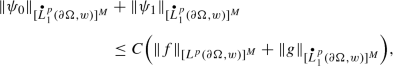  (6.186)

  for some constant C ∈ (0, ∞) independent of f and g. In particular, u^± in (6.185) also satisfy (6.184).

  Finally, for any given q ∈ (1, ∞) and ω ∈ A_q(∂ Ω, σ) ( after possibly further decreasing δ ∈ (0, 1) relative to q and $[\omega ]_{A_q}$) one has

  

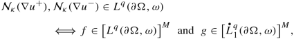  (6.187)

  and if either of these conditions holds then

  

  (6.188)

• (c) [ Sharpness ] Fix some transmission parameter $\eta \in {\mathbb {C}}\setminus \{-1\}$. Then even for L =  Δ and $\Omega ={\mathbb {R}}^n_{+}$, if $A\notin {\mathfrak {A}}_{L}^{\mathrm {dis}}$ it may happen that the Transmission Problem (6.178) fails to be solvable when p = 2 and w ≡ 1.

• (d) [ Well-Posedness for η = 1] In the case when

  

  (6.189)

  the Transmission Problem (6.178) is solvable, and any two solutions of the Transmission Problem (6.178) differ by a constant. Any solution is given by

  $$\displaystyle \begin{aligned} \begin{array}{l} u^{+}:={\mathcal{D}}^{+}_{{}_{A,\mathrm{mod}}}g-{\mathscr{S}}^{+}_{{}_{\mathrm{mod}}}f+c\,\,\mathit{\mbox{ in }}\,\,\Omega_{+}, \\ {} u^{-}:=-{\mathcal{D}}^{-}_{{}_{A,\mathrm{mod}}}g-{\mathscr{S}}^{-}_{{}_{\mathrm{mod}}}f+c\,\,\mathit{\mbox{ in }}\,\,\Omega_{-}, \end{array} \end{aligned} $$

  (6.190)

  for some $c\in {\mathbb {C}}^M$, where the superscripts ± indicate that the modified layer potentials are associated with the sets Ω_± introduced in (6.177). In addition, any solution satisfies (6.184).

A few clarifications pertaining to the nature of the above theorem are in order here. First, Lemma 2.3 and definitions imply that

(6.191)

In particular, this makes it meaningful to talk about the nontangential boundary trace $u^{-}\big |{ }_{\partial \Omega }^{{ }^{\kappa -\mathrm {n.t.}}}$, here understood as $u^{-}\big |{ }_{\partial (\Omega _{-})}^{{ }^{\kappa -\mathrm {n.t.}}}$. Second, the existence of $u^{\pm }\big |{ }_{\partial \Omega }^{{ }^{\kappa -\mathrm {n.t.}}}$ at σ-a.e. point on ∂ Ω is an implicit demand in the formulation of the Transmission Problem (6.178). Third, the conormal derivative $\partial ^A_\nu u^{+}$ is defined as in (3.66), while in light of the last property in (6.191) we take $\partial ^A_\nu u^{-}$ to be the opposite of (i.e.,− 1 times) the conormal derivative operator from (3.66) for the domain Ω₋ acting on the function u⁻, i.e.,

$$\displaystyle \begin{aligned} \partial^A_\nu u^{-}:=-\partial^A_{(-\nu)}u^{-}. \end{aligned} $$

(6.192)

Collectively, (2.576), (2.48), (3.66), and the Fatou-type result from Theorem 3.4 imply that the conormal derivatives $\partial ^A_\nu u^{\pm }$ are well defined in the context of (6.178).

We now turn to the task of proving Theorem 6.15.

Proof of Theorem 6.15

As regards item (a), we need to address the issue of uniqueness (modulo constants) in either of the scenarios specified in (6.179)–(6.180), assuming that Ω is a δ-AR domain for some sufficiently small δ ∈ (0, 1). In all cases, the goal is to show that

(6.193)

Let us first justify (6.193) in the case when (6.179) holds. Suppose u^± solve the homogeneous version of the Transmission Problem (6.178). Assuming that Ω is a δ-AR domain with δ ∈ (0, 1) sufficiently small, Theorem 2.3, Propositions 2.24, 2.22 (keeping in mind (2.576)), and the homogeneous version of the first boundary condition in (6.178), to the effect that

$$\displaystyle \begin{aligned} u^{+}\big|{}_{\partial\Omega}^{{}^{\kappa-\mathrm{n.t.}}}=u^{-}\big|{}_{\partial\Omega}^{{}^{\kappa-\mathrm{n.t.}}} \,\,\mbox{ at }{\sigma}\mbox{-a.e. point on }\,\,\partial\Omega, \end{aligned} $$

(6.194)

for each j, k ∈{1, …, n}, allow us to write

$$\displaystyle \begin{aligned} \nu_j\Big((\partial_ku^{+})\big|{}^{{}^{\kappa-\mathrm{n.t.}}}_{\partial\Omega}\Big) &-\nu_k\Big((\partial_ju^{+})\big|{}^{{}^{\kappa-\mathrm{n.t.}}}_{\partial\Omega}\Big) =\partial_{\tau_{jk}}\Big(u^{+}\big|{}^{{}^{\kappa-\mathrm{n.t.}}}_{\partial\Omega}\Big) \\ {} &=\partial_{\tau_{jk}}\Big(u^{-}\big|{}^{{}^{\kappa-\mathrm{n.t.}}}_{\partial\Omega}\Big) =\nu_j\Big((\partial_ku^{-})\big|{}^{{}^{\kappa-\mathrm{n.t.}}}_{\partial\Omega}\Big) -\nu_k\Big((\partial_ju^{-})\big|{}^{{}^{\kappa-\mathrm{n.t.}}}_{\partial\Omega}\Big) \end{aligned} $$

(6.195)

at σ-a.e. point on ∂ Ω. In terms of the abbreviation introduced in (6.125) we agree to recast this as

$$\displaystyle \begin{aligned} \begin{array}{c} \partial_{\,T_{jk}}u^{+}_\alpha=\partial_{\,T_{jk}}u^{-}_\alpha\,\,\mbox{ at }{\sigma}\mbox{-a.e. point on }\,\,\partial\Omega, \\ {} \mbox{for each }{j,k\in\{1,\dots,n\}}\mbox{ and }{\alpha\in\{1,\dots,M\}}. \end{array} \end{aligned} $$

(6.196)

Also, from (6.62) (written for u⁺ and Ω₊), (6.196), the fact that we are presently assuming

$$\displaystyle \begin{aligned} \partial^A_\nu u^{+}=\eta\cdot\partial^A_\nu u^{-}, \end{aligned} $$

(6.197)

and (6.63) (written for u⁻ and Ω₋) we see that for each integer ℓ ∈{1, …, n} and each γ ∈{1, …, M}, and each point x ∈ Ω we have

$$\displaystyle \begin{aligned} (\partial_\ell u^{+}_\gamma)(x) &=\int_{\partial\Omega} a^{\beta\alpha}_{rs}(\partial_r E_{\gamma\beta})(x-y)\big(\partial_{\,T_{\ell s}}u^{+}_\alpha\big)(y)\,\mbox{d}\sigma(y) \\ {} &\quad -\int_{\partial\Omega}(\partial_\ell E_{\gamma\alpha})(x-y)\big(\partial^A_\nu u^{+}\big)_\alpha(y)\,\mbox{d}\sigma(y) \\ {} &=\int_{\partial\Omega} a^{\beta\alpha}_{rs}(\partial_r E_{\gamma\beta})(x-y)\big(\partial_{\,T_{\ell s}}u^{-}_\alpha\big)(y)\,\mbox{d}\sigma(y) \\ {} &\quad -\eta\int_{\partial\Omega}(\partial_\ell E_{\gamma\alpha})(x-y)\big(\partial^A_\nu u^{-}\big)_\alpha(y)\,\mbox{d}\sigma(y) \\ {} &=(1-\eta)\int_{\partial\Omega}(\partial_\ell E_{\gamma\alpha})(x-y)\big(\partial^A_\nu u^{-}\big)_\alpha(y)\,\mbox{d}\sigma(y). \end{aligned} $$

(6.198)

Granted this, the same type of argument which, starting with (6.83), has produced (6.88) presently yields

$$\displaystyle \begin{aligned} \partial^A_\nu u^{+}=(1-\eta)\big(-\tfrac{1}{2}I+K^{\#}_{A^\top}\big)\big(\partial^A_\nu u^{-}\big) \end{aligned} $$

(6.199)

which, given that we are currently assuming $\partial ^A_\nu u^{+}=\eta \cdot \partial ^A_\nu u^{-}$ (cf. (6.197)), further implies

$$\displaystyle \begin{aligned} \left(-\tfrac{\eta+1}{2}I+(1-\eta)K^{\#}_{A^\top}\right)\big(\partial^A_\nu u^{-}\big)=0. \end{aligned} $$

(6.200)

Since we are presently assuming $A^\top \in {\mathfrak {A}}_{L^{\top }}^{\mathrm {dis}}$ and $\eta \in {\mathbb {C}}\setminus \{-1\}$, Theorem 4.8 ensures (taking δ ∈ (0, 1) sufficiently small, to begin with) that $-\tfrac {\eta +1}{2}I+(1-\eta )K^{\#}_{A^\top }$ is an invertible operator on [L^p(∂ Ω, w)]^M. Together with (6.200) this forces

$$\displaystyle \begin{aligned} \partial^A_\nu u^{-}=0. \end{aligned} $$

(6.201)

Going back with this in (6.198) then yields ∇u⁺ = 0 in Ω₊. In concert with Theorem 2.4 this goes to show that u⁺ is a constant in Ω₊, say $u^{+}\equiv c\in {\mathbb {C}}^M$ in Ω₊. Based on this and (6.194) we then conclude that

$$\displaystyle \begin{aligned} u^{-}\big|{}_{\partial\Omega}^{{}^{\kappa-\mathrm{n.t.}}}=u^{+}\big|{}_{\partial\Omega}^{{}^{\kappa-\mathrm{n.t.}}}=c \,\,\mbox{ at }{\sigma}\mbox{-a.e. point on }\,\,\partial\Omega, \end{aligned} $$

(6.202)

hence also

$$\displaystyle \begin{aligned} \nu_j\Big((\partial_ku^{-})\big|{}^{{}^{\kappa-\mathrm{n.t.}}}_{\partial\Omega}\Big) -\nu_k\Big((\partial_ju^{-})\big|{}^{{}^{\kappa-\mathrm{n.t.}}}_{\partial\Omega}\Big) =\partial_{\tau_{jk}}\Big(u^{-}\big|{}^{{}^{\kappa-\mathrm{n.t.}}}_{\partial\Omega}\Big)=0 \end{aligned} $$

(6.203)

for each j, k ∈{1, …, n} (cf. (6.195)). Keeping (6.201) and (6.203) in mind and writing (6.62) for u⁻ and Ω₋, we then see that ∇u⁻ = 0 in Ω₋. By once again relying on Theorem 2.4, we infer that u⁻ is a constant in Ω₋. In concert with (6.202) this shows that u⁻≡ c in Ω₋, finishing the proof of (6.193) under the assumptions made in (6.179).

Going further, the goal is to prove (6.193) when Ω is a δ-AR domain for some sufficiently small δ ∈ (0, 1), under the assumptions made in (6.180). As before, (6.194)–(6.196) and (6.197) are presently true. Also, from (6.62) (written for u⁺ and Ω₊), (6.196), (6.197), and (6.63) (written for u⁻ and Ω₋) we see that for each pair of indices, ℓ ∈{1, …, n} and γ ∈{1, …, M}, and each point x ∈ Ω we have

$$\displaystyle \begin{aligned} (\partial_\ell u^{+}_\gamma)(x) &=\int_{\partial\Omega} a^{\beta\alpha}_{rs}(\partial_r E_{\gamma\beta})(x-y)\big(\partial_{\,T_{\ell s}}u^{+}_\alpha\big)(y)\,\mbox{d}\sigma(y) \\ {} &\quad -\int_{\partial\Omega}(\partial_\ell E_{\gamma\alpha})(x-y)\big(\partial^A_\nu u^{+}\big)_\alpha(y)\,\mbox{d}\sigma(y) \\ {} &=\int_{\partial\Omega} a^{\beta\alpha}_{rs}(\partial_r E_{\gamma\beta})(x-y)\big(\partial_{\,T_{\ell s}}u^{-}_\alpha\big)(y)\,\mbox{d}\sigma(y) \\ {} &\quad -\eta\int_{\partial\Omega}(\partial_\ell E_{\gamma\alpha})(x-y)\big(\partial^A_\nu u^{-}\big)_\alpha(y)\,\mbox{d}\sigma(y) \\ {} &=(1-\eta)\int_{\partial\Omega}a^{\beta\alpha}_{rs}(\partial_r E_{\gamma\beta})(x-y) \big(\partial_{\,T_{\ell s}}u^{-}_\alpha\big)(y)\,\mbox{d}\sigma(y) \\ {} &=(1-\eta)\int_{\partial\Omega}a^{\beta\alpha}_{rs}(\partial_r E_{\gamma\beta})(x-y) \big(\partial_{\,T_{\ell s}}u^{+}_\alpha\big)(y)\,\mbox{d}\sigma(y). \end{aligned} $$

(6.204)

Having established this, the same type of argument which, starting with (6.122), has produced (6.130) currently gives (with the factor 1 − η absorbed in T)

$$\displaystyle \begin{aligned} \begin{array}{c} \partial_{\,T_{t\ell}}u^{+}=(1-\eta)\big(\tfrac{1}{2}I+K_{A}\big)\big(\partial_{\,T_{t\ell}}u^{+}\big) +\big[M_{\nu},T\big]\big(\partial_Tu^{+}\big) \\ {} \mbox{at }{\sigma}\mbox{-a.e. point on }{\partial\Omega}\mbox{, for each }{t,\ell\in\{1,\dots,n\}}. \end{array} \end{aligned} $$

(6.205)

Hence, for each t, ℓ ∈{1, …, n} we have

$$\displaystyle \begin{aligned} \Big(\tfrac{1+\eta}{2}\Big)\partial_{\,T_{t\ell}}u^{+}=(1-\eta)K_{A}\big(\partial_{\,T_{t\ell}}u^{+}\big) +\big[M_{\nu},T\big]\big(\partial_Tu^{+}\big)\,\,\mbox{ on }\,\,\partial\Omega. \end{aligned} $$

(6.206)

Since η ≠ − 1 and $A\in {\mathfrak {A}}_{L}^{\mathrm {dis}}$, much as in (6.131)–(6.134) this forces

$$\displaystyle \begin{aligned} \partial_{\,T_{t\ell}}u^{+}_\alpha=0\,\,\mbox{ for each }\,\,t,\ell\in\{1,\dots,n\}\,\,\mbox{ and }\,\,\alpha\in\{1,\dots,M\} \end{aligned} $$

(6.207)

if δ ∈ (0, 1) is sufficiently small to begin with. Feeding this back into (6.204) then proves that ∇u⁺ = 0 in Ω₊, hence (cf. Theorem 2.4), u⁺ is a constant in Ω₊, say

$$\displaystyle \begin{aligned} u^{+}\equiv c^{+}\in{\mathbb{C}}^M\,\,\mbox{ in }\,\,\Omega_{+}. \end{aligned} $$

(6.208)

Based on this, (6.197), (6.195), and keeping in mind that η ≠ 0, we then obtain

$$\displaystyle \begin{aligned} \begin{array}{c} \partial^A_\nu u^{-}=\eta^{-1}\cdot\partial^A_\nu u^{+}=0\,\,\mbox{ at }{\sigma}\mbox{-a.e. point on }\,\,\partial\Omega, \\ {} \mbox{and }\,\,\partial_{\,T_{jk}}u^{-}_\alpha=0\,\,\mbox{ at }{\sigma}\mbox{-a.e. point on }\,\,\partial\Omega, \\ {} \mbox{for each }{j,k\in\{1,\dots,n\}}\mbox{ and }{\alpha\in\{1,\dots,M\}}. \end{array} \end{aligned} $$

(6.209)

With this in hand, the integral representation formula (6.62) written for u⁻ in Ω₋, then shows that ∇u⁻ = 0 in Ω₋ thus, as before, the function u⁻ is a constant in Ω₋, say $u^{-}=c^{-}\in {\mathbb {C}}^M$ in Ω₋. The final step is to invoke equality (6.194) to write $c^{+}=u^{+}\big |{ }_{\partial \Omega }^{{ }^{\kappa -\mathrm {n.t.}}}=u^{-}\big |{ }_{\partial \Omega }^{{ }^{\kappa -\mathrm {n.t.}}}=c^{-}$, which completes the proof of (6.193) under the assumptions made in (6.180). This completes the treatment of item (a).

To deal with the claims in item (b), work under the assumptions made in (6.181), i.e., $A\in {\mathfrak {A}}_L^{\mathrm {dis}}$, $A^\top \in {\mathfrak {A}}_{L^{\top }}^{\mathrm {dis}}$, and $\eta \in {\mathbb {C}}\setminus \{-1\}$. Then Theorems 4.8 and 4.11 ensure the existence of some threshold δ ∈ (0, 1), whose nature is as specified in the statement of the present theorem, such that if ${\left \lVert \nu \right \rVert }_{[\mathrm {BMO}(\partial \Omega ,\sigma )]^n}<\delta$ it follows that the operators

$$\displaystyle \begin{aligned} -\tfrac{\eta+1}{2}I+(\eta-1)K^{\#}_{A^\top}:\big[L^p(\partial\Omega,w)\big]^M\longrightarrow\big[L^p(\partial\Omega,w)\big]^M, \end{aligned} $$

(6.210)

and

(6.211)

are invertible. Assuming this is the case, it is meaningful to define u^± as in (6.182)–(6.183). In view of (6.191) and item (c) in Proposition 3.5 (used both for Ω₊ and Ω₋), these functions satisfy the first three conditions in (6.178), the estimates claimed in (6.184), and we have (keeping (6.192) and (6.191) in mind)

$$\displaystyle \begin{aligned} \partial^A_\nu u^{+}-\eta\cdot\partial^A_\nu u^{-} &=\big(-\tfrac{1}{2}I+K^{\#}_{A^\top}\big)h_0+\big(-\tfrac{1}{2}I+K^{\#}_{A^\top}\big)h_1 \\ {} &\quad -\eta(-1)\big(-\tfrac{1}{2}I-K^{\#}_{A^\top}\big)h_0 \\ {} &=\left(-\tfrac{\eta+1}{2}I+(1-\eta)K^{\#}_{A^\top}\right)h_0+\big(-\tfrac{1}{2}I+K^{\#}_{A^\top}\big)h_1 \\ {} &=f-\big(-\tfrac{1}{2}I+K^{\#}_{A^\top}\big)h_1+\big(-\tfrac{1}{2}I+K^{\#}_{A^\top}\big)h_1 \\ {} &=f\,\,\mbox{ at }{\sigma}\mbox{-a.e. point on }\,\,\partial\Omega. \end{aligned} $$

(6.212)

Finally, thanks to (3.42)–(3.47), (2.575), and (6.191), we see that

$$\displaystyle \begin{aligned} u^{+}\big|{}_{\partial\Omega}^{{}^{\kappa-\mathrm{n.t.}}} -u^{-}\big|{}_{\partial\Omega}^{{}^{\kappa-\mathrm{n.t.}}} &=S_{{}_{\mathrm{mod}}}h_0+S_{{}_{\mathrm{mod}}}h_1+c-S_{{}_{\mathrm{mod}}}h_0 \\ {} &=S_{{}_{\mathrm{mod}}}h_1+c=g \,\,\mbox{ at }{\sigma}\mbox{-a.e. point on }\,\,\partial\Omega. \end{aligned} $$

(6.213)

Hence, the functions u^± defined as in (6.182)–(6.183) solve the Transmission Problem (6.178) and satisfy the estimates demanded in (6.184).

An alternative proof of the solvability of the Transmission Problem (6.178) in the case when $A\in {\mathfrak {A}}_{L}^{\mathrm {dis}}$, $A^\top \in {\mathfrak {A}}_{L^{\top }}^{\mathrm {dis}}$, and $\eta \in {\mathbb {C}}\setminus \{-1\}$, which now employs double layers in the integral representation of the solution, goes as follows. First, item (2) in Theorem 4.13 guarantees that the operator (4.392) is surjective. Together with the Open Mapping Theorem this implies that, for some constant C ∈ (0, ∞),

(6.214)

Also, since $A\in {\mathfrak {A}}_{L}^{\mathrm {dis}}$ and $\eta \in {\mathbb {C}}\setminus \{-1\}$, from Theorem 4.12 we see that

(6.215)

is an invertible operator. Consequently, there exists such that

$$\displaystyle \begin{aligned} \big(-\tfrac{\eta+1}{2}I+(1-\eta)K_{{}_{A,\mathrm{mod}}}\big)\psi_1=g-\big(\tfrac{1}{2}I+K_{{}_{A,\mathrm{mod}}}\big)k-c \end{aligned} $$

(6.216)

for some constant $c\in {\mathbb {C}}^M$, and

(6.217)

for some constant C ∈ (0, ∞) independent of f, g. To proceed, introduce

(6.218)

and, finally, define the functions u^± as in (6.185) for these choices of ψ₀, ψ₁, and c. Then Theorem 3.5 gives that $u^{\pm }\in \big [{\mathscr {C}}^{\infty }(\Omega _{\pm })\big ]^M$ satisfy Lu^± = 0 in Ω_± and ${\mathcal {N}}_{\kappa }(\nabla u^{\pm })\in L^p(\partial \Omega ,w)$. Moreover,

$$\displaystyle \begin{aligned} u^{+}\big|{}_{\partial\Omega}^{{}^{\kappa-\mathrm{n.t.}}}-u^{-}\big|{}_{\partial\Omega}^{{}^{\kappa-\mathrm{n.t.}}} &=\big(\tfrac{1}{2}I+K_{{}_{A,\mathrm{mod}}}\big)\psi_0+c -\big(\tfrac{1}{2}I-K_{{}_{A,\mathrm{mod}}}\big)\psi_1 \\ {} &=\big(\tfrac{1}{2}I+K_{{}_{A,\mathrm{mod}}}\big)(k-\eta\cdot\psi_1)+c -\big(\tfrac{1}{2}I-K_{{}_{A,\mathrm{mod}}}\big)\psi_1 \\ {} &=\big(\tfrac{1}{2}I+K_{{}_{A,\mathrm{mod}}}\big)k +\big(-\tfrac{\eta+1}{2}I+(1-\eta)K_{{}_{A,\mathrm{mod}}}\big)\psi_1+c \\ {} &=(g-c)+c=g, \end{aligned} $$

(6.219)

by (6.185), (3.134), and (6.216) (keeping in mind (6.191)). In addition,

$$\displaystyle \begin{aligned} \partial^A_\nu u^{+}-\eta\cdot\partial^A_\nu u^{-} &=\big(\partial^A_\nu{\mathcal{D}}_{{}_{A,\mathrm{mod}}}\big)\psi_0 +\eta\big(\partial^A_\nu{\mathcal{D}}_{{}_{A,\mathrm{mod}}}\big)\psi_1 \\ {} &=\big(\partial^A_\nu{\mathcal{D}}_{{}_{A,\mathrm{mod}}}\big)(\psi_0+\eta\cdot\psi_1) =\big(\partial^A_\nu{\mathcal{D}}_{{}_{A,\mathrm{mod}}}\big)k=f, \end{aligned} $$

(6.220)

thanks to (6.192), (3.135), and (6.214). This goes to show that (u⁺, u⁻) is, as claimed, a solution of the Transmission Problem (6.178). Furthermore, the estimate recorded in (6.186) is a consequence of (6.214), (6.217), (6.218), and Theorem 3.6.

At this stage, all claims pertaining to existence and estimates in item (b) have been established. The fact that, in the current setting, any two solutions of the Transmission Problem (6.178) differ by a constant is a consequence of the assumptions in (6.181) and item (a). As regards additional integrability properties for the solution of the Transmission Problem (6.178), the right-pointing implication in (6.187) together with the right-pointing inequality in (6.188) are consequences of (6.74) and the fact that we have

$$\displaystyle \begin{aligned} \begin{array}{c} |f|=\big|\partial^A_\nu u^{+}-\eta\cdot\partial^A_\nu u^{-}\big| \leq C\big({\mathcal{N}}_{\kappa}(\nabla u^{+})+{\mathcal{N}}_{\kappa}(\nabla u^{-})\big) \\ {} \mbox{at }{\sigma}-\mbox{a.e. point on }{\partial\Omega}. \end{array} \end{aligned} $$

(6.221)

The left-pointing implication in (6.187) along with the left-pointing inequality in (6.188) are seen from (7.290), (6.182), (4.342), Remarks 4.21, 4.22, Theorem 3.5, and Proposition 3.5.

Let us now justify the claim made in item (c). Fix some arbitrary transmission parameter $\eta \in {\mathbb {C}}\setminus \{-1\}$. Also, pick a coefficient matrix $A=(a_{jk})_{1\leq j,k\leq n}\in {\mathbb {C}}^{n\times n}$ whose entries satisfy

$$\displaystyle \begin{aligned} a_{jk}+a_{kj}=2\delta_{jk}\,\,\mbox{ for each }\,\,j,k\in\{1,\dots,n\}. \end{aligned} $$

(6.222)

This condition simply ensures that

$$\displaystyle \begin{aligned} \Delta=a_{jk}\partial_j\partial_k. \end{aligned} $$

(6.223)

The goal is to show that we may choose a coefficient matrix A as above together with some boundary datum $f\in L^2({\mathbb {R}}^{n-1},{\mathcal {L}}^{n-1})$ such that the Transmission Problem

$$\displaystyle \begin{aligned} \left\lbrace \begin{array}{l} u^{\pm}\in{\mathscr{C}}^{\infty}({\mathbb{R}}^n_{\pm}), \\ {} \Delta u^{\pm}=0\,\,\mbox{ in }\,\,{\mathbb{R}}^n_{\pm}, \\ {} {\mathcal{N}}_{\kappa}(\nabla u^{\pm})\in L^2({\mathbb{R}}^{n-1},{\mathcal{L}}^{n-1}), \\ {} u^{+}\big|{}_{\partial{\mathbb{R}}^n_{+}}^{{}^{\kappa-\mathrm{n.t.}}}-u^{-}\big|{}_{\partial{\mathbb{R}}^n_{-}}^{{}^{\kappa-\mathrm{n.t.}}} =0\,\,\mbox{ at }{{\mathcal{L}}^{n-1}}\mbox{-a.e. point on }\,\,{\mathbb{R}}^{n-1}, \\ {} \partial^A_\nu u^{+}-\eta\cdot\partial^A_\nu u^{-}=f\,\,\mbox{ at }{{\mathcal{L}}^{n-1}}\mbox{-a.e. point on }\,\,{\mathbb{R}}^{n-1} \\ {} \end{array} \right. \end{aligned} $$

(6.224)

does not have a solution. To this end, observe that the first three conditions above guarantee that there exists a function $h\in L^2({\mathbb {R}}^{n-1},{\mathcal {L}}^{n-1})$ such that

$$\displaystyle \begin{aligned} u^{\pm}={\mathscr{S}}_{{}_{\mathrm{mod}}}h\,\,\mbox{ in }\,\,{\mathbb{R}}^n_{\pm}. \end{aligned} $$

(6.225)

Indeed, if A_o := I_n×n, then the function $f_o:=\partial ^{A_o}_\nu u^{+}-\eta \cdot \partial ^{A_o}_\nu u^{-}$ belongs to $L^2({\mathbb {R}}^{n-1},{\mathcal {L}}^{n-1})$ and u^± solve the Transmission problem (6.178) in the case when L =  Δ, $\Omega ={\mathbb {R}}^n_{+}$, p = 2, w ≡ 1, and corresponding to the boundary data g := 0 and f := f_o. Then what we have proved in item (b) (cf. (6.182)–(6.183)) implies (6.225). Granted (6.225), using the last boundary condition in (6.224) and reasoning as in (6.212) shows that we have

$$\displaystyle \begin{aligned} f &=\partial^A_\nu u^{+}-\eta\cdot\partial^A_\nu u^{-} =\big(-\tfrac{1}{2}I+K^{\#}_{A^\top}\big)h-\eta(-1)\big(-\tfrac{1}{2}I-K^{\#}_{A^\top}\big)h \\ {} &=\left(-\tfrac{\eta+1}{2}I+(1-\eta)K^{\#}_{A^\top}\right)h\,\,\mbox{ at }{{\mathcal{L}}^{n-1}}\mbox{-a.e. point on }\,\,{\mathbb{R}}^{n-1}. \end{aligned} $$

(6.226)

Thus, in order for the Transmission Problem (6.224) to be solvable, f must necessarily be in the range of the operator $\tfrac {\eta +1}{2(\eta -1)}I+K^{\#}_{A^\top }$ acting on $L^2({\mathbb {R}}^{n-1},{\mathcal {L}}^{n-1})$. As such, in order to find an example for which the Transmission Problem (6.224) may not be solvable for arbitrary boundary data f in $L^2({\mathbb {R}}^{n-1},{\mathcal {L}}^{n-1})$, it suffices to produce an example of a coefficient matrix $A=(a_{jk})_{1\leq j,k\leq n}\in {\mathbb {C}}^{n\times n}$ whose entries satisfy (6.222) for which the operator $\tfrac {\eta +1}{2(\eta -1)}I+K^{\#}_{A^\top }$ fails to be surjective on $L^2({\mathbb {R}}^{n-1},{\mathcal {L}}^{n-1})$. In this regard, first note that, straight from definitions, for any function $\phi \in L^2({\mathbb {R}}^{n-1},{\mathcal {L}}^{n-1})$ we have

(6.227)

where E_Δ is the standard fundamental solution for the Laplacian (cf. (3.404)), and where R_j is the j-th Riesz transform in ${\mathbb {R}}^{n-1}$. In view of this, we may reformulate our goal as the task of finding a coefficient matrix $A=(a_{jk})_{1\leq j,k\leq n}\in {\mathbb {C}}^{n\times n}$ whose entries satisfy (6.222) for which the operator

$$\displaystyle \begin{aligned} T:=\frac{\eta+1}{\eta-1}I+\sum_{j=1}^{n-1}a_{jn}R_j \end{aligned} $$

(6.228)

fails to be surjective on $L^2({\mathbb {R}}^{n-1},{\mathcal {L}}^{n-1})$. Bring in the Fourier transform ${\mathcal {F}}'$ in ${\mathbb {R}}^{n-1}$. Since, as is well known (see, e.g., [102, (4.9.15), p. 183]), for each given function $\phi \in L^2({\mathbb {R}}^{n-1},{\mathcal {L}}^{n-1})$ and each j ∈{1, …, n − 1} we have

$$\displaystyle \begin{aligned} {\mathcal{F}}'\big(R_j\phi\big)(\xi')=(-\mbox{i})\frac{\xi_j}{|\xi'|}\big({\mathcal{F}}'\phi\big)(\xi'), \qquad \xi'\in{\mathbb{R}}^{n-1}\setminus\{0\}, \end{aligned} $$

(6.229)

it follows that

$$\displaystyle \begin{aligned} {\mathcal{F}}'\big(T\phi\big)=m{\mathcal{F}}'\phi\,\,\mbox{ for each }\,\,\phi\in L^2({\mathbb{R}}^{n-1},{\mathcal{L}}^{n-1}), \end{aligned} $$

(6.230)

where, for each $xi'=(\xi _1,\dots ,\xi _{n-1})\in {\mathbb {R}}^{n-1}\setminus \{0\}$, we have set

$$\displaystyle \begin{aligned} m(\xi'):=\frac{\eta+1}{\eta-1}+(-\mbox{i})\sum_{j=1}^{n-1}\frac{a_{jn}\xi_j}{|\xi'|}. \end{aligned} $$

(6.231)

Thanks to (6.230) and Plancherel’s theorem, the operator T is surjective if and only if m only vanishes of a set of Lebesgue measure zero in ${\mathbb {R}}^{n-1}$ and 1∕m is essentially bounded in ${\mathbb {R}}^{n-1}$. To prevent T from being surjective, it therefore suffices to choose A so that m vanishes somewhere in ${\mathbb {R}}^{n-1}\setminus \{0\}$. For example, this is the case whenever

$$\displaystyle \begin{aligned} \begin{array}{c} A=I_{n\times n}+C\,\,\mbox{ with }\,\,C=(c_{jk})_{1\leq j,k\leq n}\in{\mathbb{C}}^{n\times n} \\ {} \mbox{satisfying }\,\,C^\top=-C\,\,\mbox{ as well as }\,\,(c_{jn})_{1\leq j\leq n-1}\in i\,S^{n-2}. \end{array} \end{aligned} $$

(6.232)

In particular, this precludes A from being the identity, hence from being a distinguished coefficient tensor for the Laplacian. Ultimately, the conclusion is that, even for L =  Δ and $\Omega ={\mathbb {R}}^n_{+}$, if $A\notin {\mathfrak {A}}_{L}^{\mathrm {dis}}$ then the Transmission Problem (6.178) may fail to be solvable when p = 2 and w ≡ 1. This concludes the treatment of item (c).

To deal with the claims in item (d), suppose for the remainder of the proof that η = 1 and that Ω is a two-sided NTA domain with an unbounded Ahlfors regular boundary. Consider u^± defined as in (6.190). Since we are presently assuming that Ω is a UR domain, from Theorem 3.5 and item (c) in Proposition 3.5 we see that $u^{\pm }\in \big [{\mathscr {C}}^{\infty }(\Omega _{\pm })\big ]^M$ satisfy Lu^± = 0 in Ω_± as well as ${\mathcal {N}}_{\kappa }(\nabla u^{\pm })\in L^p(\partial \Omega ,w)$. In addition,

$$\displaystyle \begin{aligned} u^{+}\big|{}_{\partial\Omega}^{{}^{\kappa-\mathrm{n.t.}}}-u^{-}\big|{}_{\partial\Omega}^{{}^{\kappa-\mathrm{n.t.}}} &=\big(\tfrac{1}{2}I+K_{{}_{A,\mathrm{mod}}}\big)g-S_{{}_{A,\mathrm{mod}}}f \\ {} &\quad -\big(-\tfrac{1}{2}I+K_{{}_{A,\mathrm{mod}}}\big)g+S_{{}_{A,\mathrm{mod}}}f=g, \end{aligned} $$

(6.233)

by (3.134) and (3.47) (also keeping in mind (2.575)). Also,

$$\displaystyle \begin{aligned} \partial^A_\nu u^{+}-\partial^A_\nu u^{-} &=\big(\partial^A_\nu{\mathcal{D}}_{{}_{A,\mathrm{mod}}}\big)g-\big(-\tfrac{1}{2}I+K^{\#}_{A^\top}\big)f \\ {} &\quad -\big(\partial^A_\nu{\mathcal{D}}_{{}_{A,\mathrm{mod}}}\big)g+\big(\tfrac{1}{2}I+K^{\#}_{A^\top}\big)f=f, \end{aligned} $$

(6.234)

thanks to (6.192), (3.126), and (3.135). The conclusion is that (u⁺, u⁻) is indeed a solution of the Transmission Problem (6.178).

Let us next justify (6.193) in the case when (6.189) holds (hence η = 1 and Ω is a two-sided NTA domain with an unbounded Ahlfors regular boundary). To this end, assume u^± solve the homogeneous version of the Transmission Problem (6.178) formulated with η = 1. The off-diagonal Carleson measure estimate of reverse Hölder type from Proposition 2.5 ensures the existence of a constant C ∈ (0, ∞) with the property that for every point x ∈ ∂ Ω and every radius r ∈ (0, ∞) we have

(6.235)

In concert with (2.525), this permits us to estimate

(6.236)

for every x ∈ ∂ Ω and every r ∈ (0, ∞); in particular,

$$\displaystyle \begin{aligned} \begin{array}{c} \nabla u^{\pm}\in\big[L^{np/(n-1)}(\Omega_{\pm}\cap B(x,r),{\mathcal{L}}^n)\big]^{M\cdot n} \\ {} \mbox{for each }{x\in\partial\Omega}\mbox{ and }{r\in(0,\infty)}. \end{array} \end{aligned} $$

(6.237)

Likewise, from Proposition 2.5 and (2.525) we see that there exists some constant C ∈ (0, ∞) such that for every point x ∈ ∂ Ω and every radius r ∈ (0, ∞) we have

(6.238)

since (cf. (6.178) and (6.74))

$$\displaystyle \begin{aligned} {\mathcal{N}}^{Cr}_{\kappa}u\in L^p_{\mathrm{loc}}(\partial\Omega,w). \end{aligned} $$

(6.239)

In particular,

$$\displaystyle \begin{aligned} \begin{array}{c} u^{\pm}\in\big[L^{np/(n-1)}(\Omega_{\pm}\cap B(x,r),{\mathcal{L}}^n)\big]^M \\ {} \mbox{for each }{x\in\partial\Omega}\mbox{ and }{r\in(0,\infty)}. \end{array} \end{aligned} $$

(6.240)

Also, if we consider the function defined ${\mathcal {L}}^n$-a.e. in ${\mathbb {R}}^n$ as

$$\displaystyle \begin{aligned} u:=\left\{ \begin{array}{ll} u^{+} &\mbox{ in }\,\,\Omega_{+}, \\ {} u^{-} &\mbox{ in }\,\,\Omega_{-}, \end{array} \right. \end{aligned} $$

(6.241)

then u is ${\mathcal {L}}^n$-measurable and (6.238) implies that

$$\displaystyle \begin{aligned} u\in\big[L^{np/(n-1)}_{\mathrm{loc}}({\mathbb{R}}^n,{\mathcal{L}}^n)\big]^M \hookrightarrow\big[L^1_{\mathrm{loc}}({\mathbb{R}}^n,{\mathcal{L}}^n)\big]^M. \end{aligned} $$

(6.242)

Let (ν₁, …, ν_n) denote the scalar components of the geometric measure theoretic outward unit normal ν to Ω. Then for each index j ∈{1, …, n} and each vector-valued test function $\varphi \in \big [{\mathscr {C}}^{\infty }_0({\mathbb {R}}^n)\big ]^M$, we may compute (with the first two pairings considered in the sense of distributions in ${\mathbb {R}}^n$)

$$\displaystyle \begin{aligned} \langle\partial_j u,\varphi\rangle &=-\langle u,\partial_j\varphi\rangle =-\int_{{\mathbb{R}}^n}\langle u,\partial_j\varphi\rangle\,\mbox{d}{\mathcal{L}}^n \\ {} &=-\int_{\Omega_{+}}\langle u^{+},\partial_j\varphi\rangle\,\mbox{d}{\mathcal{L}}^n -\int_{\Omega_{-}}\langle u^{-},\partial_j\varphi\rangle\,\mbox{d}{\mathcal{L}}^n \\ {} &=\int_{\Omega_{+}}\langle\partial_j u^{+},\varphi\rangle\,\mbox{d}{\mathcal{L}}^n -\int_{\partial\Omega}\nu_j\big\langle\big(u^{+}\big|{}_{\partial\Omega}^{{}^{\kappa-\mathrm{n.t.}}}\big),\varphi\big\rangle\,\mbox{d}\sigma \\ {} &\quad +\int_{\Omega_{-}}\langle\partial_j u^{-},\varphi\rangle\,\mbox{d}{\mathcal{L}}^n +\int_{\partial\Omega}\nu_j\big\langle\big(u^{-}\big|{}_{\partial\Omega}^{{}^{\kappa-\mathrm{n.t.}}}\big),\varphi\big\rangle\,\mbox{d}\sigma \\ {} &=\int_{\Omega_{+}}\langle\partial_j u^{+},\varphi\rangle\,\mbox{d}{\mathcal{L}}^n +\int_{\Omega_{-}}\langle\partial_j u^{-},\varphi\rangle\,\mbox{d}{\mathcal{L}}^n. \end{aligned} $$

(6.243)

Above, the fourth equality is provided by the integration by parts formula proved in [111, §1.7], whose present applicability is ensured by (6.178), (6.74), (6.237), (6.240), and the fact that (6.239) together with (2.576) imply

$$\displaystyle \begin{aligned} {\mathcal{N}}^{Cr}_{\kappa}u\in L^1_{\mathrm{loc}}(\partial\Omega,\sigma)\,\,\mbox{ for each }\,\,r\in(0,\infty). \end{aligned} $$

(6.244)

Also, the last equality in (6.243) uses (6.191) and the fact that we are currently assuming $u^{+}\big |{ }_{\partial \Omega }^{{ }^{\kappa -\mathrm {n.t.}}}=u^{-}\big |{ }_{\partial \Omega }^{{ }^{\kappa -\mathrm {n.t.}}}$. In turn, from (6.243) and (6.237) we conclude that, with the derivatives computed in the sense of distributions, for each j ∈{1, …, n} we have

$$\displaystyle \begin{aligned} \partial_j u\in\big[L^{np/(n-1)}_{\mathrm{loc}}({\mathbb{R}}^n,{\mathcal{L}}^n)\big]^M \end{aligned} $$

(6.245)

and, in fact,

$$\displaystyle \begin{aligned} \partial_j u=\left\{ \begin{array}{ll} \partial_j u^{+} &\mbox{ in }\,\,\Omega_{+}, \\ {} \partial_j u^{-} &\mbox{ in }\,\,\Omega_{-}. \end{array} \right. \end{aligned} $$

(6.246)

Moreover, combining (6.246) with (6.236) shows that there exists some constant C ∈ (0, ∞) with the property that for every x ∈ ∂ Ω and every r ∈ (0, ∞) we have

(6.247)

To proceed, consider now an arbitrary point $x\in {\mathbb {R}}^n$ and pick some x_∗∈ ∂ Ω such that dist(x, ∂ Ω) = |x − x_∗|. Since B(x, r) ⊆ B(x_∗, 2r) for each r > dist(x, ∂ Ω), we conclude from (6.247) that there exists C ∈ (0, ∞) such that

(6.248)

for every point $x\in {\mathbb {R}}^n$ and every radius r > dist(x, ∂ Ω), where x_∗∈ ∂ Ω is such that dist(x, ∂ Ω) = |x − x_∗|.

We next claim that

$$\displaystyle \begin{aligned} {Lu=0}\mbox{ in the sense of distributions in }{{\mathbb{R}}^n}. \end{aligned} $$

(6.249)

To justify this, pick an arbitrary vector-valued test function $\varphi \in \big [{\mathscr {C}}^{\infty }_0({\mathbb {R}}^n)\big ]^M$ and write (with the first two pairings considered in the sense of distributions in ${\mathbb {R}}^n$)

$$\displaystyle \begin{aligned} \langle Lu,\varphi\rangle &=\langle u,L^\top\varphi\rangle =\int_{{\mathbb{R}}^n}\langle u,L^\top\varphi\rangle\,\mbox{d}{\mathcal{L}}^n \\ {} &=\int_{\Omega_{+}}\langle u^{+},L^\top\varphi\rangle\,\mbox{d}{\mathcal{L}}^n +\int_{\Omega_{-}}\langle u^{-},L^\top\varphi\rangle\,\mbox{d}{\mathcal{L}}^n \\ {} &=\int_{\Omega_{+}}\langle Lu^{+},\varphi\rangle\,\mbox{d}{\mathcal{L}}^n +\int_{\partial\Omega}\big\langle u^{+}\big|{}_{\partial\Omega}^{{}^{\kappa-\mathrm{n.t.}}},\partial_\nu^{A^\top}\varphi\big\rangle\,\mbox{d}\sigma -\int_{\partial\Omega}\big\langle\partial_\nu^{A}u^{+},\varphi\big\rangle\,\mbox{d}\sigma \\ {} &\quad +\int_{\Omega_{-}}\langle Lu^{-},\varphi\rangle\,\mbox{d}{\mathcal{L}}^n -\int_{\partial\Omega}\big\langle u^{-}\big|{}_{\partial\Omega}^{{}^{\kappa-\mathrm{n.t.}}},\partial_\nu^{A^\top}\varphi\big\rangle\,\mbox{d}\sigma +\int_{\partial\Omega}\big\langle\partial_\nu^{A}u^{-},\varphi\big\rangle\,\mbox{d}\sigma \\ {} &=0. \end{aligned} $$

(6.250)

The fourth equality in (6.250) is a consequence of the Green type formula for second-order systems established in [113, §1.7], whose present applicability is guaranteed by (6.178), (6.74), Theorem 3.4, (6.237), (6.240), and the fact that (6.239) together with (2.576) entail

$$\displaystyle \begin{aligned} {\mathcal{N}}_{\kappa}(\nabla u)\in L^1_{\mathrm{loc}}(\partial\Omega,\sigma)\,\,\mbox{ and }\,\, {\mathcal{N}}^{Cr}_{\kappa}u\in L^1_{\mathrm{loc}}(\partial\Omega,\sigma)\,\,\mbox{ for all }\,\,r\in(0,\infty). \end{aligned} $$

(6.251)

In addition, the last equality in (6.250) uses (6.178), (6.191), plus the fact that we are now assuming $u^{+}\big |{ }_{\partial \Omega }^{{ }^{\kappa -\mathrm {n.t.}}} =u^{-}\big |{ }_{\partial \Omega }^{{ }^{\kappa -\mathrm {n.t.}}}$ and $\partial ^A_\nu u^{+}=\partial ^A_\nu u^{-}$. This establishes (6.250) which, in turn, proves (6.249).

As a consequence of (6.249) and elliptic regularity, $u\in \big [{\mathscr {C}}^{\infty }({\mathbb {R}}^n)\big ]^M$. In particular, for each index j ∈{1, …, n} we have $\partial _j u\in \big [{\mathscr {C}}^{\infty }({\mathbb {R}}^n)\big ]^M$ as well as L(∂_ju) = ∂_j(Lu) = 0, since L has constant coefficients. Bearing this in mind, interior estimates for weakly elliptic systems proved in [102, Theorem 11.12, p. 415] give

(6.252)

for every point $x\in {\mathbb {R}}^n$ and every radius r ∈ (0, ∞). Together with (6.248) this implies

$$\displaystyle \begin{aligned} |(\nabla &u)(x)| \\ {} &\leq\frac{C[w]_{A_p}^{1/p}}{w\big(\partial\Omega\cap B(x_\ast,Cr)\big)^{\frac{1}{p}}} \Big(\big\|{\mathcal{N}}_{\kappa}(\nabla u^{+})\big\|{}_{L^p(\partial\Omega,w)} +\big\|{\mathcal{N}}_{\kappa}(\nabla u^{-})\big\|{}_{L^p(\partial\Omega,w)}\Big) \end{aligned} $$

(6.253)

for every point $x\in {\mathbb {R}}^n$ and every radius r > dist(x, ∂ Ω), where x_∗∈ ∂ Ω is such that dist(x, ∂ Ω) = |x − x_∗|. At this stage, upon recalling (2.540) and the fact that ${\mathcal {N}}_{\kappa }(\nabla u^{\pm })\in L^p(\partial \Omega ,w)$ (cf. (6.178)), after passing to limit r →∞ in (6.253) we arrive at the conclusion that

$$\displaystyle \begin{aligned} (\nabla u)(x)=0\,\,\mbox{ for each point }\,\,x\in{\mathbb{R}}^n. \end{aligned} $$

(6.254)

Hence, u is constant in ${\mathbb {R}}^n$, from which (6.193) readily follows on account of (6.241). This finishes the proof of (6.193) under the assumption made in (6.189).

The proof of Theorem 6.15 is therefore complete. □

We continue by making a series of remarks aimed at further exploring the nature of Theorem 6.15.

Remark 6.11

In various special circumstances, the statement of Theorem 6.15 may be further streamlined. For example, Theorem 3.8 gives that if the system L actually satisfies the strong Legendre–Hadamard ellipticity condition then in place of either set of conditions specified in (6.179), (6.180), (6.181) we may simply assume

$$\displaystyle \begin{aligned} {A\in{\mathfrak{A}}_{L}^{\mathrm{dis}}}\mbox{ and }{\eta\in{\mathbb{C}}\setminus\{-1\}}. \end{aligned} $$

(6.255)

Also, if n ≥ 3, M = 1, and the matrix $A\in {\mathfrak {A}}_L$ is symmetric then, thanks to (3.223), either set of conditions specified in (6.179), (6.180), (6.255) may simply be replaced by just the demand that $\eta \in {\mathbb {C}}\setminus \{-1\}$.

Remark 6.12

There is another boundary value problem, closely related to the Transmission Problem (6.178), in which the transmission parameter shows up in the formulation of the Dirichlet boundary condition (as opposed to the Neumann boundary condition, as was the case in (6.178)). Specifically, retaining the background assumptions made in Theorem 6.15 now consider

(6.256)

When η ≠ 0, working with the functions v⁺ := u⁺ in Ω₊ and v⁻ := η ⋅ u⁻ in Ω₋, matters are readily reduced to the “standard” Transmission Problem (6.178) written with η⁻¹ in place of η. When η = 0 it follows that (6.256) decouples into a Homogeneous Regularity Problem for the function u⁺ in Ω₊, and a Neumann Problem for the function u⁻ in Ω₋ with boundary datum $\partial ^A_\nu u^{+}-f$. In particular, we have solvability results for (6.256) which are similar to those in Theorem 6.15.

Remark 6.13

Much as in the case of the Tangential Derivative Problem (6.97), we may re-fashion the Transmission Problem (6.178) as

$$\displaystyle \begin{aligned} \left\lbrace \begin{array}{l} u^{\pm}\in\big[{\mathscr{C}}^{\infty}(\Omega_{\pm})\big]^M, \\ {} Lu^{\pm}=0\,\,\mbox{ in }\,\,\Omega_{\pm}, \\ {} {\mathcal{N}}_{\kappa}(\nabla u^{\pm})\in L^p(\partial\Omega,w), \\ {} \Big\{\nu_j\Big((\partial_ku^{+})\big|{}^{{}^{\kappa-\mathrm{n.t.}}}_{\partial\Omega}\Big) -\nu_k\Big((\partial_ju^{+})\big|{}^{{}^{\kappa-\mathrm{n.t.}}}_{\partial\Omega}\Big)\Big\} \\ {} \quad -\Big\{\nu_j\Big((\partial_ku^{-})\big|{}^{{}^{\kappa-\mathrm{n.t.}}}_{\partial\Omega}\Big) -\nu_k\Big((\partial_ju^{-})\big|{}^{{}^{\kappa-\mathrm{n.t.}}}_{\partial\Omega}\Big)\Big\} =\partial_{\tau_{jk}}g, \\ {} \,\,\mbox{ at }{\sigma}-\mbox{a.e. point on }{\partial\Omega},\mbox{ for each }\,\,j,k\in\{1,\dots,n\}, \\ {} \partial^A_\nu u^{+}-\eta\cdot\partial^A_\nu u^{-}=f\in\big[L^p(\partial\Omega,w)\big]^M, \\ {} \end{array} \right. \end{aligned} $$

(6.257)

where the function g is arbitrarily specified in , the homogeneous Muckenhoupt weighted boundary Sobolev space defined in (2.598). For this boundary value problem, similar results as in Theorem 6.15 continue to be valid.

Remark 6.14

Under the same background assumptions made in Theorem 6.15 (and with the same conventions adopted there), it is of interest to single out the special case corresponding to having g = 0 in (6.178), i.e., consider the following Reduced Transmission Problem:

$$\displaystyle \begin{aligned} \left\lbrace \begin{array}{l} u^{\pm}\in\big[{\mathscr{C}}^{\infty}(\Omega_{\pm})\big]^M, \\ {} Lu^{\pm}=0\,\,\mbox{ in }\,\,\Omega_{\pm}, \\ {} {\mathcal{N}}_{\kappa}(\nabla u^{\pm})\in L^p(\partial\Omega,w), \\ {} u^{+}\big|{}_{\partial\Omega}^{{}^{\kappa-\mathrm{n.t.}}} =u^{-}\big|{}_{\partial\Omega}^{{}^{\kappa-\mathrm{n.t.}}}\,\,\mbox{ at }{\sigma}\mbox{-a.e. point on }\,\,\partial\Omega, \\ {} \partial^A_\nu u^{+}-\eta\cdot\partial^A_\nu u^{-}=f\in\big[L^p(\partial\Omega,w)\big]^M. \\ {} \end{array} \right. \end{aligned} $$

(6.258)

Running the same argument as in the proof of Theorem 6.15, this time we no longer need to assume that the operator in (6.211) is an isomorphism, ultimately allows us to impose lighter demands on the nature of the system L and the coefficient tensor A. Specifically, now working under the sole assumption that $A^\top \in {\mathfrak {A}}_{L^{\top }}^{\mathrm {dis}}$ and $\eta \in {\mathbb {C}}\setminus \{-1\}$, the same proof as before shows that there exists δ ∈ (0, 1) which depends only on n, p, $[w]_{A_p}$, A, η, and the Ahlfors regularity constant of ∂ Ω such that if ${\left \lVert \nu \right \rVert }_{[\mathrm {BMO}(\partial \Omega ,\sigma )]^n}<\delta$ (hence the set Ω is a δ-AR domain) then the operator $-\tfrac {\eta +1}{2}I+(1-\eta )K^{\#}_{A^\top }$ is invertible on the Muckenhoupt weighted Lebesgue space [L^p(∂ Ω, w)]^M and the functions $u^{\pm }:\Omega _{\pm }\to {\mathbb {C}}^M$ defined as

$$\displaystyle \begin{aligned} u^{\pm}(x):=\Big({\mathscr{S}}_{{}_{\mathrm{mod}}}\left(-\tfrac{\eta+1}{2}I+(1-\eta)K^{\#}_{A^\top}\right)^{-1}f\Big)(x) \,\,\mbox{ for }\,\,x\in\Omega_{\pm} \end{aligned} $$

(6.259)

solve the Reduced Transmission Problem formulated in (6.258) and satisfy, for some constant C ∈ (0, ∞) independent of f,

$$\displaystyle \begin{aligned} {\left\lVert {\mathcal{N}}_{\kappa}(\nabla u^{\pm}) \right\rVert}_{L^p(\partial\Omega,w)}\leq C{\left\lVert f \right\rVert}_{[L^p(\partial\Omega,w)]^M}. \end{aligned} $$

(6.260)

Moreover, the result established in item (a) of Theorem 6.15 working under the hypotheses in (6.179) gives uniqueness (modulo constants) for the Reduced Transmission Problem (6.258). Hence, well posedness follows by simply assuming that $A^\top \in {\mathfrak {A}}^{\mathrm {dis}}_{L^\top }$.

Remark 6.15

Once again, for familiar reasons, a similar solvability result to the one established in Theorem 6.15 turns out to be true for the Transmission Problem with data in Lorentz spaces, i.e., for

(6.261)

with p ∈ (1, ∞) and q ∈ (0, ∞], where is the Lorentz-based homogeneous Sobolev space defined in an analogous fashion to (2.598). The reader is referred to Theorem 7.23 (and also Examples 8.2, 8.6) for more general results of this type.

Remark 6.16

Thanks to (3.228)–(3.229), Theorem 6.15 is applicable to the Lamé system L_μ,λ = μ Δ + (λ + μ)∇div in ${\mathbb {R}}^n$ with n ≥ 2, assuming μ ≠ 0, 2μ + λ ≠ 0, 3μ + λ ≠ 0, provided we work with the coefficient tensor A(ζ) defined as in (3.226) for the choice $\zeta =\frac {\mu (\mu +\lambda )}{3\mu +\lambda }$. In addition, when n = 2, we may rely on the invertibility result from Theorem 4.14 (and duality) to conclude that the transmission boundary problem for the two-dimensional Lamé system in sufficiently flat Ahlfors regular domains in the plane is solvable when formulated in a similar fashion to (6.178) with A := A(ζ) and $\eta \in {\mathbb {C}}\setminus \{\pm 1\}$, for a larger range of ζ’s, namely

$$\displaystyle \begin{aligned} \zeta\in{\mathbb{C}}\setminus\Big\{\pm\frac{\eta+1}{\eta-1}\Big[\frac{2\mu(2\mu+\lambda)}{3\mu+\lambda}\Big] +\frac{\mu(\mu+\lambda)}{3\mu+\lambda}\Big\}. \end{aligned} $$

(6.262)

Remark 6.17

The case of the Transmission Problem for the Laplacian in upper-graph Lipschitz domains in ${\mathbb {R}}^n$, with n ≥ 2 arbitrary, has been treated in [46]. In the two-dimensional setting, for L =  Δ the Laplacian and Ω an infinite sector in the plane, counterexamples to the well-posedness of the Transmission Problem (6.178) for certain values of p (related to the aperture of Ω and the transmission parameter appearing in the formulation of the problem) have been given in [105].

Remark 6.18

It is of interest to observe that

(6.263)

Indeed, if u⁻ is such that

$$\displaystyle \begin{aligned} \left\lbrace \begin{array}{l} u^{-}\in\big[{\mathscr{C}}^{\infty}(\Omega_{-})\big]^M, \\ {} Lu^{-}=0\,\,\mbox{ in }\,\,\Omega_{-}, \\ {} {\mathcal{N}}_{\kappa}(\nabla u^{-})\in L^p(\partial\Omega,w), \\ {} u^{-}\big|{}_{\partial\Omega}^{{}^{\kappa-\mathrm{n.t.}}}=c\,\,\mbox{ at }{\sigma}\mbox{-a.e. point on }\,\,\partial\Omega, \\ {} \end{array} \right. \end{aligned} $$

(6.264)

for some constant $c\in {\mathbb {C}}^M$, then setting u⁺ := c in Ω₊ yields a pair (u⁺, u⁻) which is a null-solution of the Transmission Problem (6.178) formulated for η = 0.

There are two scenarios under which uniqueness (modulo constants) for the Transmission Problem (6.178) has been established in item (a) of Theorem 6.15. First, it was assumed that (6.179) holds and, in this case, condition ${\mathfrak {A}}_{L^{\top }}^{\mathrm {dis}}\neq \varnothing$ alone ensures uniqueness (modulo constants) for the Homogeneous Regularity Problem for the system L in Ω₋, as noted in item (b) of Theorem 6.8. Second, when (6.180) is assumed, in principle it may happen that the Homogeneous Regularity Problem for the system L in Ω₋ lacks uniqueness (modulo constants). However, this time (as opposed to (6.179)), we are asking that η ≠ 0, so the issue singled out in (6.263) becomes a moot point. This is a heuristic explanation of the perceived asymmetry in the manner in which the sets of hypotheses (6.179) and (6.180) have been formulated.

It is possible to enhance the solvability result from Theorem 6.15 via perturbations, and our next theorem elaborates on this aspect.

Theorem 6.16

Retain the original background assumptions on the set Ω from Theorem 6.15 and, as before, fix an integrability exponent p ∈ (1, ∞) along with a Muckenhoupt weight w ∈ A_p(∂ Ω, σ) and a transmission parameter $\eta \in {\mathbb {C}}\setminus \{-1\}$. Consider a system $L_o\in \mathfrak {L}^{\mathrm {dis}}$ with $L_o^\top \in \mathfrak {L}^{\mathrm {dis}}$ ( cf. (3.195)) , and fix some $A_o\in \mathfrak {A}^{\mathrm {dis}}_{L_o}$.

Then there exist a threshold δ ∈ (0, 1) and an open neighborhood ${\mathcal {U}}$ of A_o in $\mathfrak {A}$, both of which depend only on n, η, p, $[w]_{A_p}$, A_o, and the Ahlfors regularity constant of ∂ Ω, with the property that if ${\left \lVert \nu \right \rVert }_{[\mathrm {BMO}(\partial \Omega ,\sigma )]^n}<\delta$ ( i.e., if Ω is a δ-AR domain) then for each coefficient tensor $A\in {\mathcal {U}}$ the Transmission Problem (6.178) formulated for the system L_A ( cf. (3.7)) and the conormal derivative associated with A ( cf. (3.66)) is actually solvable, and any two solutions differ by a constant from ${\mathbb {C}}^M$.

Proof

This is seen by reasoning as in the proofs of Theorems 6.4 and 6.15, keeping in mind Theorem 3.9. □

We may also establish solvability results for the version of the Reduced Transmission Problem (6.258) now formulated for boundary data belonging to sums of Muckenhoupt weighted Lebesgue spaces.

Theorem 6.17

Let $\Omega \subseteq {\mathbb {R}}^{n}$ be a UR domain. Abbreviate $\sigma :={\mathcal {H}}^{n-1}\lfloor \partial \Omega$ and fix an aperture parameter κ > 0. Also, pick a pair of integrability exponents p₀, p₁ ∈ (1, ∞) along with a pair of Muckenhoupt weights $w_0\in A_{p_0}(\partial \Omega ,\sigma )$ and $w_1\in A_{p_1}(\partial \Omega ,\sigma )$. Finally, consider a homogeneous, second-order, constant complex coefficient, M × M weakly elliptic system L in ${\mathbb {R}}^n$, and select some coefficient tensor $A\in {\mathfrak {A}}_L$.

Then similar results, concerning existence, integral representation formulas, estimates, additional integrability properties, and well-posedness, as in Theorem 6.15 , are valid for the Reduced Transmission Problem

$$\displaystyle \begin{aligned} \left\lbrace \begin{array}{l} u^{\pm}\in\big[{\mathscr{C}}^{\infty}(\Omega_{\pm})\big]^M, \\ {} Lu^{\pm}=0\,\,\mathit{\mbox{ in }}\,\,\Omega_{\pm}, \\ {} {\mathcal{N}}_{\kappa}(\nabla u^{\pm})\in L^{p_0}(\partial\Omega,w_0)+L^{p_1}(\partial\Omega,w_1), \\ {} u^{+}\big|{}_{\partial\Omega}^{{}^{\kappa-\mathrm{n.t.}}} =u^{-}\big|{}_{\partial\Omega}^{{}^{\kappa-\mathrm{n.t.}}}\,\,\mathit{\mbox{ at }}{\sigma}\mathit{\mbox{-a.e. point on }}\,\,\partial\Omega, \\ {} \partial^A_\nu u^{+}-\eta\cdot\partial^A_\nu u^{-}=f\in\big[L^{p_0}(\partial\Omega,w_0)+L^{p_1}(\partial\Omega,w_1)\big]^M. \\ {} \end{array} \right. \end{aligned} $$

(6.265)

Proof

Existence, estimates, and an integral representation formula are all established reasoning as in the proof of Theorem 6.15, using the fact that the operator $-\tfrac {\eta +1}{2}I+(1-\eta )K^{\#}_{A^\top }$ is invertible on the space $\big [L^{p_0}(\partial \Omega ,w_0)+L^{p_1}(\partial \Omega ,w_1)\big ]^M$ under the assumption made in item (b) of Theorem 6.15 (see Proposition 4.2). For uniqueness (modulo constants), we reason much as in the treatment of item (a) in Theorem 6.15, working under the hypotheses in (6.179). Specifically, (6.194)–(6.200) goes through since $L^{p_0}(\partial \Omega ,w_0)+L^{p_1}(\partial \Omega ,w_1)$ embeds into the space $L^1\big (\partial \Omega ,\frac {\sigma (x)}{1+|x|{ }^{n-1}}\big )$ (cf. (2.575)), and then (4.336) used in concert with (6.200) gives (6.201). The rest is as before, and the conclusion is that any null-solution of (6.265) is a pair of identical constants. □

References

L. Escauriaza, M. Mitrea, Transmission problems and spectral theory for singular integral operators on Lipschitz domains. J. Funct. Anal. 216(1), 141–171 (2004)
L. Grafakos, Classical and Modern Fourier Analysis (Pearson Education, New Jersey, 2004)
N. Kalton, M. Mitrea, Stability of Fredholm properties on interpolation scales of quasi-Banach spaces and applications. Trans. Am. Math. Soc. 350, 3837–3901 (1998)
V.A. Kozlov, V.G. Maz’ya, J. Rossmann, Elliptic Boundary Value Problems in Domains with Point Singularities. Mathematical Surveys and Monographs, vol. 52 (American Mathematical Society, Providence, 1997)
V.A. Kozlov, V.G. Maz’ya, J. Rossmann, Spectral Problems Associated with Corner Singularities of Solutions to Elliptic Equations. Mathematical Surveys and Monographs, vol. 85 (American Mathematical Society, Providence, 2001)
D. Mitrea, Distributions, Partial Differential Equations, and Harmonic Analysis. Universitext, 2nd edn. (Springer, New York, 2018)
I. Mitrea, K. Ott, Counterexamples to the well-posedness of Lp transmission boundary value problems for the Laplacian. Proc. Am. Math Soc. 135(7), 2037–2043 (2007)
D. Mitrea, I. Mitrea, M. Mitrea, Geometric Harmonic Analysis-Volume I: A Sharp Divergence Theorem with Nontangential Pointwise Traces, Developments in Mathematics, 72 (Springer, Cham, 2022)
D. Mitrea, I. Mitrea, M. Mitrea, Geometric Harmonic Analysis-Volume III: Integral Representations, Calderón-Zygmund Theory, Fatou Theorems, and Applications to Scattering, 74 Developments in Mathematics (Springer, Cham, 2022)
D. Mitrea, I. Mitrea, M. Mitrea, Geometric Harmonic Analysis-Volume IV: Boundary Layer Potentials in Uniformly Rectifiable Domains, and Applications to Complex Analysis, Developments in Mathematics, 75 (Springer, Cham, 2023)
Z. Shen, Weighted estimates for elliptic systems on Lipschitz domains. Indiana Univ. Math. J. 55(3), 1135–1154 (2006)
T. Toro, Potential analysis meets geometric measure theory, in Proceedings of the International Congress of Mathematicians 2010, ICM 2010 (2011), pp. 1485–1497
Author information
Authors and Affiliations
Rights and permissions
Copyright information
© 2022 The Author(s), under exclusive license to Springer Nature Switzerland AG
About this chapter
Cite this chapter
Marín, J., Martell, J., Mitrea, D., Mitrea, I., Mitrea, M. (2022). Boundary Value Problems in Muckenhoupt Weighted Spaces. In: Singular Integral Operators, Quantitative Flatness, and Boundary Problems. Progress in Mathematics, vol 344. Birkhäuser, Cham. https://doi.org/10.1007/978-3-031-08234-4_6
Download citation
DOI: https://doi.org/10.1007/978-3-031-08234-4_6
Published:
Publisher Name: Birkhäuser, Cham
Print ISBN: 978-3-031-08233-7
Online ISBN: 978-3-031-08234-4
eBook Packages: Mathematics and StatisticsMathematics and Statistics (R0)