
Abstract
At present, it appears that systems of pneumatic units with discrete and analog control, in which the required analog law of motion of the output member is provided with the help of discrete switchgear, offer a promising potential. When developing the schemes of positional hydraulic-pneumatic units, the parameters of the movement of the hydraulic-pneumatic unit are studied, namely: the value of displacement, speed, and acceleration of its output member. To carry out the simulation, a design based on discrete switchgear was taken as the basis for the pneumatic positional unit. Solving the inverse problem, i.e., with the law of motion of the output member of the pneumatic unit (specifying the positioning function) known, we determine the mandatory law of change in the effective areas of the control line and represent each equation of the dynamic model as block diagrams. A mathematical model of the system of pneumatic positional units with program control was developed. It considers the features of the system of pneumatic units and consists of mathematical models of the actuator, a real-time control line model, and a real-time control system. The proposed algorithm for analysis of dynamic characteristics using the MATLAB simulation environment confirms the adequacy of the mathematical models describing the operation of a positional pneumatic unit implemented on discrete pneumatic equipment. The developed algorithm is advisable to analyze the operation of the existing one and for designing new technological equipment.
Access provided by Autonomous University of Puebla. Download conference paper PDF
Keywords
1 Introduction
The basic requirements for hydropneumatic positional units are known. They ensure the specified technical characteristics determined by the technological process, ease of manufacture and cost-effectiveness; high reliability and trouble-free operation; the ability to reprogram the control system quickly.
When developing pneumatic positional units, designers are faced with the problem of a limited choice in the range of manufacturers of pneumatic valves with proportional electric control. Therefore, at present, the most promising are systems of pneumatic units with discrete and analog control, i.e., those in which the required analog law of motion of the output member is provided using discrete switchgear. Due to the discreteness of choice in the controlled parameters, the interconnection with digital control devices is facilitated. These systems focused on regulating the working environment in the cavities of the hydraulic and pneumatic motor, allowing to expand of the functionality of hydraulic units. The apparent advantage of such systems is that they can be relatively easy to implement [1,2,3]. The effectiveness of these control methods is determined by the constant improvement of the control system, which is currently based on microprocessor-based computer technology, allowing applying complex control algorithms [4,5,6].
2 Literature Review
Recently, digital hydraulic and pneumatic units have been widely used in the industry [7, 8]. These systems are logically integrable in the spirit of the Industry 4.0 strategy, according to which these systems can be combined into one network [9], communicate with each other in real-time, self-adjust, and learn new behavior models [10, 11].
The active implementation of digital pneumatic units into the industry is facilitated by the relative simplicity of design and operation, long service life, reliable operation in a low-temperature range in high humidity, dustiness, radiation of the environment, and fire and explosion safety. Digital hydraulic units allow us to increase the positioning accuracy of actuators and increase the system’s energy efficiency [12, 13].
When developing the schemes of positional hydraulic-pneumatic units, the parameters of the movement of the hydraulic-pneumatic unit are studied, namely: the value of displacement, speed, and acceleration of its output member. Studies [14,15,16] show that the main tasks of developers of systems of controlled hydraulic-pneumatic units are associated with the fulfillment of the requirements for the movement of the output member, which led to a variety of methods for controlling the motion parameters of the systems of positional parts [17,18,19].
The purpose of this work is to develop an algorithm for analyzing the positioning function, which allows you to provide the specified technical characteristics of the pneumatic positional unit by describing the necessary law of change in the effective areas of the control line of the pneumatic positioning unit, implemented on discrete/digital switchgear.
3 Research Methodology
A design based on discrete switchgear was taken as the basis for the positional pneumatic unit [20, 21]. The diagram of the pneumatic unit is shown in Fig. 1.

Diagram of positioning pneumatic unit.
The pneumatic unit consists of the following elements (Fig. 1): 1 - position sensor; 2, 3 - pneumatic valves; 4 - pneumatic throttle valve; 5 - pneumatic cylinder.
Based on differential equations describing the dynamic characteristics of the pneumatic unit during operation and calculation [22], a dynamic model of the pneumatic unit was created. The designations of the variables used in the dynamic model are shown in Table 1.
System of differential equations describing a dynamic model:
where at p1 = pm and p2 = pa values of \(K_{G}^{1}\) and \(K_{G}^{2}\) become:
Solving the inverse problem, i.e., the law of motion of the output member of the pneumatic unit (specifying the positioning function) known, we determine the required law of change in the effective areas of the control line. In the case of the extension of the actuator, the effective area in the pressure line \(f_{1}^{e}\) is set and constant. Then there is the need to determine the change law in the effective area of the discharge line. Thus, the system of differential equations becomes:
4 Results
We represent each equation of the dynamic model as block diagrams [23]:
-
1.
A block diagram for solving the inverse problem of the dynamics of the positional pneumatic unit (system of differential Eqs. (2)) is shown in Fig. 2.
Fig. 2. 
Block diagram for solving the inverse problem of the dynamics of a pneumatic positional unit.
Positioning function U is shown in (Fig. 3).
Fig. 3. 
Positioning function U.
Acceleration a, speed V and movement x of the output member are shown in (Fig. 4).
Fig. 4. 
Values of the effective area in the control line at the outlet \(f_{2}^{e}\) to obtain the required law of motion of the output member; \(\dot{x}_{z}\) - specified speed of movement; \(\dot{x}\) - an obtained speed of movement.
The results show high accuracy of coincidence of the specified and actual speeds.
-
2.
The block diagram for calculating the pressure p1 from the dependence \(\dot{p}_{1} = \frac{k}{{F_{1} x + V_{10} }}\left( {f_{1}^{e} K_{G}^{1} - p_{1} F_{1} \dot{x}} \right)\) is shown in Fig. 5.
Fig. 5. 
Block diagram for calculating the pressure p1.
-
3.
The block diagram for calculating the coefficient \(K_{G}^{1}\) from dependence \(K_{G}^{1} = \mu_{1} {\text{p}}_{m} \sqrt {2RT} \phi \left( {\frac{{p_{1} }}{{p_{m} }}} \right)\), taking into account the connection diagram of the pneumatic cylinder is shown in Fig. 6.
-
4.
The block diagram for finding the effective area in the control line at the outlet \(f_{2}^{e}\) from dependence \(f_{2}^{e} = \frac{{\dot{p}_{2} \left( {F_{2} \left( {S - x} \right) + V_{20} } \right)}}{{k \cdot K_{G}^{2} }} - \frac{{p_{2} F_{2} \dot{x}}}{{K_{G}^{2} }}\) is shown in Fig. 7.
Fig. 6. 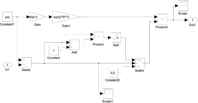
Block diagram for calculating the coefficient \(K_{G}^{1}\).
Fig. 7. 
Block diagram for calculating the effective area in the control line at the output \(f_{2}^{e}\).
-
5.
The block diagram for calculating the coefficient \(K_{G}^{2}\) from dependence \(K_{G}^{2} = - \mu_{2} {\text{p}}_{2} \sqrt {2RT} \phi \left( {\frac{{p_{a} }}{{p_{2} }}} \right)\) considering the connection diagram of the pneumatic cylinder is shown in Fig. 8.
Fig. 8. 
Block diagram for calculating the coefficient \(K_{G}^{2}\).


5 Conclusions
The developed mathematical model of the positional pneumatic unit system with program control allows considering the characteristics of the pneumatic unit system. It includes calculation models of the simulator, real-time control line mode, and real-time control mode system.
The proposed algorithm of analysis of dynamic characteristics using the MATLAB simulation environment confirms the adequacy of the mathematical models describing the operation of the positional pneumatic unit implemented on discrete pneumatic equipment. The developed algorithm is advisable to analyze the operation of the existing and new technological equipment design.
The laws of motion of the positional pneumatic unit output member are obtained. They are based on the developed algorithm of analysis of the positioning function and implemented in the MATLAB environment. Research results can provide the specified technical characteristics for a smooth acceleration of the pneumatic unit output member. Besides, formulated laws of motion allow movement at a steady speed and smooth braking with a stop at the positioning point.
References
Sokol, Y., Cherkashenko, M.: Synthesis of control schemes of drives system. NTU “KhPI” Publ., Kharkiv (2018)
Zhou, Y., Li, Y.: PLC control system of pneumatic manipulator automatic assembly line based on cloud computing platform. J. Phys. Conf. Ser. 1744, 022011 (2021)
Chelabi, M.A., Basova, Y., Hamidou, M.K., Dobrotvorskiy, S.: Analysis of the three-dimensional accelerating flow in a mixed turbine rotor. J. Eng. Sci. 8(2), D1–D7 (2021). https://doi.org/10.21272/jes.2021.8(2).d2
Filatov, D., Minav, T., Heikkine, J.: Adaptive control for direct-driven hydraulic drive. In: 11th International Fluid Power Conference, vol. 1, pp. 110–119. RWTH Aachen University, Aachen (2018)
Heikkilä, M., Linjama, M.: Fault-tolerant control of a multi-outlet digital hydraulic pump-motor. In: 11th International Fluid Power Conference, vol. 1, pp. 144–157. RWTH Aachen University, Aachen (2018)
Kanagasabai, L.: Real power loss reduction by enhanced RBS algorithm. J. Eng. Sci. 8(2), E1–E9 (2021). https://doi.org/10.21272/jes.2021.8(2).e1
Zhao, S., Li, D., Zhou, J., Sha, E.: Numerical and experimental study of a flexible trailing edge driving by pneumatic muscle actuators. J. Actuators 10(7), 142 (2021)
Cantoni, C., Gobbi, M., Mastinu, G., Meschini, A.: Brake and pneumatic wheel performance assessment – a new test rig. Measurement 150(6), 107042 (2019)
Hufnagl, H., Čebular, A., Stemler, M.: Trends in pneumatics – digitalization. In: International Conference “Fluid Power 2021”: Conference Proceedings, pp. 15–28. University Press, Maribor (2021)
Zhang, Q., Kong, X., Yu, B., Ba, K., Jin, Z., Kang, Y.: Review and development trend of digital hydraulic technology. J. Appl. Sci. 10(2), 579 (2020)
Rager, D., Neumann, R., Post, P., Murrenhoff, H.: Pneumatische antriebe für industrie 4.0 – pneumatic drives for industry 4.0. In: Mechatronik (2017)
Rager, D., Doll, M., Neumann, R., Berner, M.: New programmable valve terminal enables flexible and energy-efficient pneumatics for Industry 4.0. In: 11th International Fluid Power Conference, vol. 1, pp. 208–221. RWTH Aachen University, Aachen (2018)
Siivonen, L., Paloniitty, M., Linjama, M., Sairiala, H., Esque, S.: Digital valve system for ITER remote handling – design and prototype testing. J. Fusion Eng. Des. 146, 1637–1641 (2019)
Pavlenko, I., et al.: Effect of superimposed vibrations on droplet oscillation modes in prilling process. Processes 8(5), 566 (2020). https://doi.org/10.3390/pr8050566
Lu, S., Chen, D., Hao, R., Luo, S., Wang, M.: Design, fabrication and characterization of soft sensors through EGaIn for soft pneumatic actuators. Measurement 164(11), 107996 (2020)
Belforte, G., Mauro, S., Mattiazzo, G.: A method for increasing the dynamic performance of pneumatic servosystems with digital valves. Mechatronics 14, 1105–1120 (2004)
Pavlenko, I., Ivanov, V., Gusak, O., Liaposhchenko, O., Sklabinskyi, V.: Parameter identification of technological equipment for ensuring the reliability of the vibration separation process. In: Knapcikova, L., Balog, M., Perakovic, D., Perisa, M. (eds.) 4th EAI International Conference on Management of Manufacturing Systems. EICC, pp. 261–272. Springer, Cham (2020). https://doi.org/10.1007/978-3-030-34272-2_24
Gao, Q., Linjama, M., Paloniitty, M., Zhu, Y.: Investigation on positioning control strategy and switching optimization of an equal coded digital valve system. Proc. Inst. Mech. Eng. Part I J. Syst. Control Eng. 234(8), 959–972 (2019)
Ivanov, V., Pavlenko, I., Kuric, I., Kosov, M.: Mathematical modeling and numerical simulation of fixtures for fork-type parts manufacturing. In: Knapčíková, L., Balog, M. (eds.) Industry 4.0: Trends in Management of Intelligent Manufacturing Systems. EICC, pp. 133–142. Springer, Cham (2019). https://doi.org/10.1007/978-3-030-14011-3_12
Šitum, Ž., Benić, J., Pejić, K., Bača, M., Radić, I., Semren, D.: Design and control of mechatronic systems with pneumatic and hydraulic drive. In: International Conference “Fluid Power 2021”: Conference Proceedings, pp. 179–194. University Press, Maribor (2021)
Šitum, Ž., Benić, J., Grbić, Š., Vlahović, F., Jelenić, D., Kosor, T.: Mechatronic systems with pneumatic drive. In: International Conference “Fluid Power 2017”: Conference Proceedings, pp. 281–293. University Press, Maribor (2017)
Colombo, F., Mazza, L., Pepe, G., Raparelli, T., Trivella, A.: Inverted pendulum on a cart pneumatically actuated by means of digital valves. In: Aspragathos, N.A., Koustoumpardis, P.N., Moulianitis, V.C. (eds.) RAAD 2018. MMS, vol. 67, pp. 436–444. Springer, Cham (2018). https://doi.org/10.1007/978-3-030-00232-9_46
Elsaed, E., Abdelaziz, M., Mahmoud, N.: Investigation of a digital valve system efficiency for metering-in speed control using MATLAB/Simulink. In: International Conference on Hydraulics and Pneumatics HERVEX, 23rd edn., pp. 120–129 (2017)
Acknowledgment
The scientific results have been obtained within the research project “Fulfillment of tasks of the perspective plan of development of a scientific direction “Technical sciences” Sumy State University” ordered by the Ministry of Education and Science of Ukraine (State Reg. No. 0121U112684). The research was partially supported by the Research and Educational Center for Industrial Engineering (Sumy State University) and International Association for Technological Development and Innovations.
Author information
Authors and Affiliations
Corresponding author
Editor information
Editors and Affiliations
Rights and permissions
Copyright information
© 2022 The Author(s), under exclusive license to Springer Nature Switzerland AG
About this paper

Cite this paper
Cherkashenko, M., Gusak, O., Fatyeyev, A., Fatieieva, N., Gasiyk, A. (2022). Model of the Pneumatic Positional Unit with a Discrete Method for Control Dynamic Characteristics. In: Ivanov, V., Pavlenko, I., Liaposhchenko, O., Machado, J., Edl, M. (eds) Advances in Design, Simulation and Manufacturing V. DSMIE 2022. Lecture Notes in Mechanical Engineering. Springer, Cham. https://doi.org/10.1007/978-3-031-06044-1_8
Download citation
DOI: https://doi.org/10.1007/978-3-031-06044-1_8
Published:
Publisher Name: Springer, Cham
Print ISBN: 978-3-031-06043-4
Online ISBN: 978-3-031-06044-1
eBook Packages: EngineeringEngineering (R0)