Model Visualization Techniques and Traditional Interpretable Algorithms

Abstract

One of the easiest ways to build explainable models is by having the machine learning algorithm be intrinsically interpretable. Gaining an understanding of how well a model performs from looking at the results of model evaluation is another important way to enhance model explainability. We discuss several techniques to visualize model evaluation including precision-recall curves, ROC curves, residual plots, silhouette coefficients, and others to give a comprehensive overview of classification, regression, and clustering techniques. Next, we start understanding interpretability of some of the traditional machine learning models used in classification, regression, and clustering. The Pima Indian diabetes dataset is used to perform supervised and unsupervised classification. The insurance claims dataset is used for regression model analysis.

One of the easiest ways to build explainable models is by having the machine learning algorithm be intrinsically interpretable. Gaining an understanding of how well a model performs from looking at the results of model evaluation is another important way to enhance model explainability. We discuss several techniques to visualize model evaluation including precision-recall curves, ROC curves, residual plots, silhouette coefficients, and others to give a comprehensive overview of classification, regression, and clustering techniques. Next, we start understanding interpretability of some of the traditional machine learning models used in classification, regression, and clustering. The Pima Indian diabetes dataset is used to perform supervised and unsupervised classification. The insurance claims dataset is used for regression model analysis.

3.1 Model Validation, Evaluation, and Hyperparameters

The key to creating great models is to make sure that the model generalizes well on unseen data. Figure 3.1 gives the most well-established process that ensures models do not overfit (or underfit) and generalize well for classification and regression [HTF09a]. The labeled dataset can be divided into training, validation, and test sets from the original data. Primarily, the test set should be representative of the unseen real-world data in terms of quality, distribution, class balance, etc. If it is representative, running the model and evaluating the metrics on the test data gives an estimate close to what real-world model performance will be. Most algorithms have various parameters or options that have to be set for optimal performance. Generally, a separate validation set is used for evaluating model performance on different parameter values. In the absence of a separate validation set, splitting training data into train and validation sets is a choice and depends on the amount of labeled data and the model capacity (VC dimensions). Validation techniques like k-fold cross-validation are employed when separate validation sets are not a possibility [CT10]. The validation process plays a vital role in tuning or selecting the model parameters. The choice of these parameters affects the model performance, and hence explicitly understanding the options is critical from an explainability standpoint.

Fig. 3.1

Training, validation, and test sets for model tuning and evaluation

To compare and contrast machine learning models it is necessary to use the same split of train, validation, and test sets to evaluate all the models (with parameters) using the same performance metric(s). Interpretability is also one of the aspects that one should focus on along with other metrics.

3.1.1 Tools and Libraries

For all the tasks related to model performance analysis and visualization of results, we will use the YellowBrick package along with sklearn on the Pima Indian diabetes dataset (classification) and the insurance claims dataset (regression).

3.2 Model Selection and Visualization

Most machine learning algorithms have parameters that need to be tuned for optimal performance on a given dataset. For example, a decision tree can have different values of “max depth” and the models corresponding to each such value can exhibit a range of performance values, measured as accuracy or precision, for example. A validation set or cross-validation technique is used to tune these parameters.

3.2.1 Validation Curve

Validation curve is a plot of performance metrics such as a score with respect to different values of the parameters of the model [Bra97].

Observations:

• The validation curve as in Fig. 3.2a for Decision Tree shows that at “max depth” of 4, the classifier stabilizes to give optimum AUC of around 0.88. As the number of nodes increases, the validation score remains almost constant while the training score increases indicating overfitting.

  Fig. 3.2

  

  Validation curves for classifiers with AUC—area under ROC curve. (a) Decision tree. (b) Logistic regression

• The validation curve as in Fig. 3.2b for Logistic Regression shows best performance for the parameter C at 0.1 with AUC value around 0.77. As the C value increases the validation score drops indicating the region of overfitting.

• The variance in validation and training scores is very high in Logistic Regression as compared to Decision Tree.

3.2.2 Learning Curve

A learning curve explains the relationship between a performance metric, such as accuracy for a classifier, and the number of training samples [Per10]. The learning curve provides various diagnostic insights into the classifier such as

• 1. How many training samples does the classifier/regressor need for an optimum performance score in training and validation?

• 2. Are the samples representative of the domain?

• 3. Does the bias or the variance introduce error in the classifier/regressor?

• 4. Does the model have any overfitting or underfitting issues?

The training and validation learning curves are plotted together so we can look at the relative metrics to get the overall diagnosis for decision trees and logistic regression as shown in Fig. 3.3a and b.

Fig. 3.3

Learning curves for classifiers with AUC—area under ROC curve. (a) Decision tree. (b) Logistic regression

• A flat training and validation learning curve indicates a high chance of underfitting as it might signify no improvement and hence no learning.

• A training learning curve indicating a continuous decrease right from the start is also indicative of underfitting.

• High variability in the validation learning curve, especially with cross-validation, but not in the training learning curve indicates error due to variance rather than bias.

• High variability in the training learning curve indicates error due to bias.

• A large gap between the training and validation learning curve diverging after a point in the curve indicates the ideal split and marks the beginning of overfitting.

Observations:

• The learning curves in Fig. 3.3a for Decision Tree show that training and validation curves are separated. At about 600 samples, the validation curve trends downwards. There is a large variance in the cross-validation as compared to training indicating variance errors in predictions rather than bias errors.

• The learning curves in Fig. 3.3b for Logistic Regression show both training and validation curves following similar trends and at about 600 samples, showing divergence. Similar to the Decision tree, logistic regression also indicates variance error.

• The training learning curve for Logistic Regression also shows variability and this indicates the bias error. When compared with decision tree, it can be concluded that the non-linear decision tree algorithm performs better indicating the presence of non-linear boundaries.

• The variance in logistic regression is more than that of decision tree.

3.3 Classification Model Visualization

As discussed in the last section, model selection happens based on the agreed metrics that vary based on the domain and the nature of the application [Ras20]. For example, in some compliance-based domains in financial services, false negatives have to be minimized (recall-centric), while in other applications such as fraud detection where there are fewer resources to investigate the positive hits, false positive minimization becomes imperative (precision-centric).

Many model governance teams consider model metrics and evaluation results along with the actual model as an artifact that needs to be documented and reported. From a diagnostic and white-boxing perspective, understanding how the model performs in various scenarios is critical. This section will discuss some well-known model metrics and how they impact selection, especially of the classification models.

3.3.1 Confusion Matrix and Classification Report

As shown in Fig. 3.4, the confusion matrix is a common way to visualize the classification results on the test dataset. It acts both as a quantitative metrics provider for making decisions such as how well the model generalizes and also as a diagnostics tool to understand the model’s behavior on individual classes.

Fig. 3.4

Confusion matrix for decision tree model on diabetes classification dataset

Classification report is another view of the confusion matrix but with various metrics that highlight model behavior from an efficiency and effectiveness standpoint. As shown in Fig. 3.5, various metrics such as precision, recall, F1, and support per-class basis are given in the classification report as color-coded heatmaps for Decision Tree model.

Fig. 3.5

Classification report for decision tree model on diabetes classification dataset

By visualizing classification reports for various models on the same evaluation dataset, model behaviors can be understood in a comparative sense, as shown in Fig. 3.6a and b for Gaussian Naive Bayes and Logistic regression, respectively.

Fig. 3.6

Comparing classification reports for two models. (a) GaussianNB. (b) Logistic regression

Observations:

• Figure 3.6a shows precision for the diabetic class for the Gaussian Naive Bayes model (68.9) is slightly higher than that of Logistic Regression (68.3). The precision for the non-diabetic class for the Gaussian Naive Bayes model (85.3) is higher than that of Logistic Regression (83.2). Thus if precision is the metric, then Gaussian Naive Bayes is the model one should select.

• Figure 3.6b shows recall for the diabetic class for the Gaussian Naive Bayes model (66) is higher than that of Logistic Regression (59.6). But the recall for the non-diabetic class for Logistic Regression (87.9) is slightly higher than that of Gaussian Naive Bayes (86.9). The choice of the model then depends on the skew of the dataset and the bias towards the predictions of a particular class.

• The F1 score for Gaussian Naive Bayes for both diabetic and non-diabetic is higher than that of Logistic Regression.

• Comparing Figs. 3.5, 3.6a, and b, one can clearly see that for all the metrics such as precision, recall, and F1, the non-linear decision tree model is superior to both Gaussian Naive Bayes and Logistic Regression.

3.3.2 ROC and AUC

The Receiver Operating Characteristic (ROC) curve measures a classifier’s predictive quality, comparing and visualizing the trade-off between the model’s sensitivity and specificity. Sensitivity measures how often a model correctly generates a positive for the data that is labeled as a positive (also known as the true positive rate). Specificity measures how often a model correctly generates a negative for the data that is labeled as a negative (also known as the true negative rate). The ROC curve generates another metric computing the area under the curve (AUC) and captures the relationship between false positives and true positives [GV18].

The higher the AUC, the better the model’s generalization capability is. The ROC curve’s steepness is also crucial as it describes the maximization of the true positive rate while minimizing the false positive rate. The closer the ROC curve is to the top left corner, the better the model’s quality is overall. The closer the curve comes to the center diagonal line, the closer the model is to a random guesser.

Observations:

• Figure 3.7a and b show that the AUC for Gaussian Naive Bayes and Decision Tree for both classes are almost identical, with a value of 0.89.

  Fig. 3.7

  

  Comparing ROC curves for two models. (a) GaussianNB ROC curve. (b) Decision tree ROC curve

• Based on the steepness of the curve and closeness to the top left corner, Decision Tree seems to be a slightly better choice than Gaussian Naive Bayes

3.3.3 PRC

Precision-Recall curve measures the trade-off between the two metrics—precision and recall. Precision, measured as a ratio of true positives to the sum of true positives and false positives, is a measure of exactness or efficiency [DG06]. Recall, measured as a ratio of true positives to the sum of true positives and false negatives, is a measure of completeness or effectiveness. Average precision represents the precision-recall curve as a single metric and is computed as the weighted average of precision achieved at each threshold, where the weights are the differences in recall from the previous thresholds.

The larger the area in the Precision-Recall curve, the better is the classifier, especially when there is a huge imbalance between the classes. Higher Average Precision is normally considered a good single metric by which to select the classifier in an imbalanced dataset.

Observations:

• Figure 3.8a and b show the area under PRC for Logistic Regression is higher than that of Gaussian Naive Bayes.

  Fig. 3.8

  

  Comparing ROC curves for two classifiers. (a) GaussianNB. (b) Logistic regression

• The average precision for Logistic Regression is more than that of Gaussian Naive Bayes. Hence, in a severely imbalanced dataset, selecting Logistic regression over Gaussian Naive Bayes may seem the right choice.

3.3.4 Discrimination Thresholds

Most classifiers assign a probability for class membership to the instance to be classified. The default is to assume that a probability greater than or equal to 0.5 is for one class and below 0.5 for the other in binary classification. In classification problems with imbalanced data, the default threshold can result in suboptimal performance metrics [Che+05, Pro]. One technique to improve a classifier’s performance on imbalanced data is to tune the threshold used to map probabilities to class labels. The discrimination threshold in binary classification, sometimes called classification or decision threshold, is the probability value above which one class is predicted and below which it is the other class.

• Using the training data and creating multiple train/test sets, we run the model multiple times in order to account for the variability in the data. Then the different curves are plotted, showing median and range. The discrimination threshold is the one that achieves the best evaluation metrics in the multiple runs.

• Discrimination threshold tuning is not a hyperparameter tuning but a decision based on the trade-off between false positives and false negatives on the basis of the classifier’s probability outputs.

• Tuning the discrimination threshold gives a better trade-off between precision and recall in the precision-recall curves.

Observations:

• Figure 3.9a and b show the optimal thresholds for Gaussian Naive Bayes and Logistic Regression are 0.29 and 0.13, respectively.

  Fig. 3.9

  

  Discrimination thresholds for two classifiers on the diabetes dataset. (a) GaussianNB. (b) Logistic regression

• Gaussian Naive Bayes shows relatively large variance around the mean for the queue rate, F1, and recall while Logistic Regression around precision.

3.4 Regression Model Visualization

Regression model results need to be validated and visualized in a continuous space as compared to classification models. There are various aspects of regression models such as predictions, errors, and sensitivity to hyperparameters that can be used for diagnostics or explainability. In this section, we will discuss some common techniques employed in regression analysis.

3.4.1 Residual Plots

In regression, residual plots plot the difference between the predicted and the observed values for the target. Similar to validation curves and learning curves, residual plots are used for various diagnostics [Bel+80]. The plots can be used to understand the impact of several aspects, for example, outliers, non-linearity of the data, the assumption that the errors are independent and normally distributed and heteroscedasticity.

A good regression residual plot has a high-density of points close to 0 and scattered low density around the axis without a pattern, thus confirming the errors’ independence and normal random distribution.

Observations:

• Figure 3.10 shows the residuals for both training and testing data with a good overlap and thus there is no sample bias.

  Fig. 3.10

  

  Residual plots for linear regression

• The errors have multimodal distribution and violate the normal distribution assumption.

• There are patterns around the distribution, especially around + 1000 and −1000 value, indicating independence assumption violations.

• The negative spread of errors is more than the positive, showing presence of outliers and long tail.

3.4.2 Prediction Error Plots

Prediction error plots show the actual values against the predicted values. It also shows the plot with comparison of 45^∘ line.

Prediction error plots are used for understanding errors caused by variance in the regression model. The comparison with 45^∘ line shows if the model is underestimating or overestimating.

Observations: Figure 3.11 shows errors are not constant across values, thus variances are not constant and this violates the homoskedasticity assumption.

Fig. 3.11

Prediction error plots for linear regression

3.4.3 Alpha Selection Plots

Most regression algorithms employ some form of regularization to constrain the complexity of the model. The alpha values control the complexity of the model and cross-validation is used to select the values [HTF09b]. In Fig. 3.12a and b, alpha values that give the lowest error for Ridge Regression and Lasso Regression using cross-validation technique are plotted for the insurance dataset.

Fig. 3.12

Alpha selection based on errors. (a) Ridge regression. (b) Lasso regression

If the alpha values are high, model complexity is reduced, thus reducing the error caused by variance, resulting in an overfit model. If the alpha values are too high, the error due to bias increases, resulting in an underfit model

Observations: Ridge regression has the lowest error at alpha value of 0.195 and Lasso has lowest error at alpha value of 10.0. Lasso with high alpha values indicates an underfit model with error introduced by the bias.

3.4.4 Cook’s Distance

Cook’s distance measures an instance’s influence on the regression. The larger the influence of an instance, the higher is the likelihood of an outlier, thus influencing the regression model negatively [Coo11]. Visualizing stem plot for all training instances by their Cook’s distance score and handling instances with a score more significant than a threshold by removal or imputation is a standard best practice. Cook’s distance for ith instance from n observations is given by D _i

$$\displaystyle \begin{aligned} D_i = \frac{\sum_{j=1}^{n}(\hat{y}_j-\hat{y}_{j(i)})^2}{ps^2} \end{aligned} $$

(3.1)

Any instance with score over 4∕n, where n is the number of observations is the threshold for distance scores.

Any instances with Cook’s distance greater than 0.5 or three times the mean score need to be closely examined for their influence.

Figure 3.13 shows the plot of Cook’s distance score for the entire insurance training data.

Fig. 3.13

Cook’s distance for insurance data

Observations: There are no instances with distance score greater than 0.5 in the entire dataset. Using just the threshold based on 4∕n, around 7.28% of training data are identified as highly influential based on the Cook’s distance scores. Simply removing those instances improves the training R ² scores from 0.734 to 0.834 as shown in Fig. 3.14a and b, respectively.

Fig. 3.14

Impact of removing outliers identified from cook’s distance. (a) Model before. (b) Model after

3.5 Clustering Model Visualization

Unsupervised learning techniques such as clustering are even more difficult to diagnose or explain as compared to supervised learning since “ground truth” is often undefined. This section will discuss some techniques employed to visualize, validate, and diagnose clustering models.

One of the difficult choices in many clustering algorithms such as K-means, X-means, Expectation-Maximization, etc. is selecting number of clusters, usually symbolized by k. The choice depends on many factors such as the size of the data, dimensionality, end user’s desire and prior knowledge. The optimal choice of k is a trade-off between maximum compression of the data and maximum separation between the unseen classes or the categories.

3.5.1 Elbow Method

For the elbow method, a clustering technique is run on the dataset for a range of values for k (say from 1–10). Then for each value of k, it computes an average distortion score for all the clusters. There are many ways to compute the distortion score; a common technique calculates the sum of square distances from each point to its assigned center. The plot of k and the average distortion score in a plot resembles the arm, then the k around the elbow, the point of inflection, is chosen as an optimum k. The elbow or the knee point is detected through an algorithm that finds the point of maximum curvature in the plot.

The Calinski-Harabasz score, also known as the Variance Ratio score, is the ratio of the sum of between-clusters dispersion and intercluster dispersion. The higher the Calinski-Harabasz score, the better is the clustering performance.

Figure 3.15a and b show elbow detection using distortion and the Calinski-Harabasz method to find optimum k in the k-means for the diabetes classification data.

Fig. 3.15

Elbow Method for visualizing the optimum k for k-means clustering on the diabetes classification data. (a) Distortion scores. (b) Calinski-Harabasz score

Observations: Though the diabetes dataset has two labeled classes, both the distortion score and the Calinski-Harabasz score indicate that k = 3 is the optimum cluster size.

3.5.2 Silhouette Coefficient Visualizer

The Silhouette Coefficient is an estimate of the density of the clusters. It is computed for each instance based on two different scores as

• The mean distance between that instance and all other instances in the same cluster: a

• The mean distance between that instance and all other instances in the next nearest cluster: b

$$\displaystyle \begin{aligned} s=\frac{b-a}{max(b-a)} \end{aligned} $$

(3.2)

The Silhouette visualizer displays the silhouette coefficient for each instance on a per-cluster basis, visualizing the clusters and their density. Different plots for each value of k are shown in Fig. 3.16a, b, c, and d.

Fig. 3.16

Silhouette coefficients for k ranging from 2 to 5. (a) Silhouette coefficients for k = 2. (b) Silhouette coefficients for k = 3. (c) Silhouette coefficients for k = 4. (d) Silhouette coefficients for k = 5

The Silhouette Coefficient has a best value of 1 and worst value of −1. Values near 0 indicate overlapping clusters. Negative values generally indicate that instances have the wrong cluster assignment.

Observations: Based on the average Silhouette coefficient scores (indicated by red dotted line) for the diabetes dataset, the best k is 2 where the average score is high and there are no negative scores. The split between the two classes also seems to be in the same proportion as the original labeled class distribution.

3.5.3 Intercluster Distance Maps

Intercluster distance maps visualize an embedding space in the lower dimensions of the cluster centers. Various projection techniques such as multidimensional scaling (mds), stochastic neighbor embedding (t-sne), etc. can be used for mapping from high dimensions to two dimensions. The clusters’ memberships and sizes can be determined by a scoring method such as the number of instances belonging to each cluster and gives the clusters’ relative importance (Fig. 3.17).

Fig. 3.17

Intercluster distance maps for different values of k. (a) k = 2. (b) k = 3. (c) k = 4. (d) k = 5

Observations: Intercluster distance maps for various k using mds shows that for k = 3, based on the size, distribution and no overlaps indicate an ideal cluster size for the data.

3.6 Interpretable Machine Learning Properties

This section will detail some of the properties on which most algorithms can be compared from an interpretability standpoint.

• 1. Local or Global: Does the model provide interpretability at a single instance or local level or across the entire data space?

• 2. Linearity: Is the model capable of capturing non-linear relationships between the features?

• 3. Monotonicity Does the relationship between the feature and the target go in the same direction over the entire feature domain?

• 4. Feature Interactions: Some models capture interactions between the features while some assume independence. If captured in the right way, features interactions can increase the quality but simultaneously increase the complexity as well, thus reducing the interpretability.

• 5. Best-suited Complexity: Based on the hypothesis space of the model, what kinds of problem complexity is the algorithm best suited for?

3.7 Traditional Interpretable Algorithms

3.7.1 Tools and Libraries

Well-known open-source python packages like statsmodels and sklearn along with different data and plotting libraries were used for linear regression, logistic regression, Gaussian Naive Bayes, and Decision Tree. pgmpy is used for modeling Bayesian Network and Orange for Rule Induction.

3.7.2 Linear Regression

Linear regression is one of the oldest techniques that predicts the target using weights on the input features learned from the training data [KK62b]. The interpretation of the model becomes straightforward as the target is a linear combination of weights on the features. Thus linear regression model can be described as a linear combination of input x and a weight parameter w (that is learned during training process). In a d-dimensional input (x = [x ₁, x ₂, …, x _d]), we introduce another dimension called the bias term, x ₀, with value 1. Thus the input can be seen as $\mathbf {x} \in \{1\} \times \mathbb {R}^{d}$, and the weights to be learned are $\mathbf {w} \in \mathbb {R}^{d+1}$.

In matrix notation, the input can be represented as a data matrix $\mathbf {X} \in \mathbb {R}^{N \times (d+1)}$, whose rows are examples from the data (e.g., x _n), and the output is represented as a column vector $\mathbf {y} \in \mathbb {R}^{N}$. The process of learning via linear regression can be analytically represented as minimizing the squared error between the hypothesis function h(x _n) and the target real values y _n, as

$$\displaystyle \begin{aligned} E_{train}(h(\mathbf{x},\mathbf{w}))= \frac{1}{N}\sum_{i=0}^{d}{\big({\mathbf{w}}^{\mathrm{T}}{{\mathbf{x}}_n}- y_n\big)^2} \end{aligned} $$

(3.3)

Since the data x is given, we will write the equation in terms of weights w

$$\displaystyle \begin{aligned} E_{train}(\mathbf{w}) = \frac{1}{N}\lVert({\mathbf{X}}\mathbf{w}- \mathbf{y})^2\rVert \end{aligned} $$

(3.4)

where $\lVert ({\mathbf {X}}\mathbf {w}- \mathbf {y})^2\rVert$ is the Euclidean norm of a vector.

This is an optimization problem that requires finding the weights w _opt that minimize the training error E _train.

$$\displaystyle \begin{aligned} {\mathbf{w}}_{opt} = \operatorname*{\mbox{arg min}}_{\mathbf{w} \in \mathbb{R}^{d+1}}\ E_{train}(\mathbf{w}) \end{aligned} $$

(3.5)

The solution for the weights is given by

$$\displaystyle \begin{aligned} {\mathbf{w}}_{opt} = \big({\mathbf{X}}^{\mathrm{T}}\mathbf{X}\big)^{-1}{\mathbf{X}}^{\mathrm{T}}\mathbf{y} \end{aligned} $$

(3.6)

Linear regression makes the following assumptions that are important for model validation and interpretability

• Linearity: Linear regression assumes a linear relationship between the features and the label. In many real-world datasets this assumption may not hold true.

• Homoscedasticity: Linear regression assumes the error in the prediction will have a constant variance. This can be easily verified by plotting the results and looking at the scatter of the predictions from the linear hyperplane.

• Multicollinearity: If there is correlation between the features, the estimation of weights using linear regression is not accurate as the impact of the feature and its independence from others is lost.

Interpreting linear regression model can be summarized as below

• Increasing the continuous feature by one unit changes the estimated outcome by its weight.

• The categorical features should be transformed into multiple features. Each is encoded as a binary, 0 being the reference default and 1 is the presence of the feature. The interpretation for binary or categorical in such case is—changing the modified feature from the reference default to the other, changes the estimated outcome by the feature’s weight.

• Intercept or the constant is the output when all the continuous features are at value 0 and the categories are in the reference default (e.g., 0). Understanding intercept value becomes meaningful for interpretation when the data is scaled with mean value 0 as it represents the default weight for an instance with mean values.

• Various regression methods such as Ordinary Least Squares (OLS) give not only the weights or the coefficients per feature but also standard error(std err), t-test(t), p-value(p) and the confidence intervals. The lower the standard error, the better is the accuracy of that coefficient and p-values less than a threshold alpha level indicate a statistically significant impact of that feature on the outcome.

• The R-squared value (also known as the coefficient of determination) provides a measure of how well the regression model explains the output value it is modeling. The closer the value is to 1.0, the better the model correctly describes the data.

Figure 3.18 gives the results of fitting a linear regression model on the claims insurance dataset.

Fig. 3.18

Output of linear regression model on insurance dataset

There are various visualization techniques available for diagnosing or whiteboxing the regression. Figure 3.19 shows some of the known ways to analyze a feature age regressing with the output charges. Plot (a) which is the “Y and Fitted vs. X” graph plots the dependent variable against the predicted values with a confidence interval. Plot (b) shows the residuals of the model versus the chosen feature age. Each point in the plot is an observed value; the line represents the mean of those observed values. Plot (c) is the partial regression plot showing the relationship between the charges and the feature age conditional on the other independent features. The Component-Component plus Residual (CCPR) plot is an extension to the partial regression plot, a way to view the impact of one feature on the label by taking into account the effects of the other features. Thus it is Res + w _i x _i versus x _i where Res is the residual of the whole model.

Fig. 3.19

Four different plots for feature age. (a) Regression plot showing fitted versus actual charges. (b) Residuals w.r.t age. (c) Partial regression plot and (d) CCPR plot

Explainable properties of linear regression are shown in Table 3.1.

Table 3.1 Explainable properties of Linear regression

3.7.2.1 Regularization

Regularization is a common technique employed in many weight-based learning methods to overcome the overfitting problem. There are many regularization techniques, of which we will highlight three of the most effective ones [HTF09b, HK00a].

Ridge regression or weight decay or L ₂ norm is a regularization technique where less relevant features get weights close to 0 [HK00b]. The modified solution for regression can be written as

$$\displaystyle \begin{aligned} {\mathbf{w}}_{opt} = \operatorname*{\mbox{arg min}}_{\mathbf{w} \in \mathbb{R}^{d+1}}\ \big(E_{train}(\mathbf{w}) + \lambda {\mathbf{w}}^{\mathrm{T}}\mathbf{w}\big) \end{aligned} $$

(3.7)

$$\displaystyle \begin{aligned} {\mathbf{w}}_{opt} = \big({\mathbf{X}}^{\mathrm{T}}\mathbf{X} + \lambda\mathbf{I}\big)^{-1}{\mathbf{X}}^{\mathrm{T}}\mathbf{y} \end{aligned} $$

(3.8)

where the regularization parameter λ is a hyperparameter and is generally a small value close to 0.

Lasso regression or L ₁ norm is another popular regularization used in weight-based algorithms [HTF09b]. The modified equation for L ₁ norm is

(3.9)

The absolute function in the above equation does not yield a closed-form solution and is represented as a constrained optimization problem as given below:

$$\displaystyle \begin{aligned} \operatorname*{\mbox{arg min}}_{\mathbf{w} \in \mathbb{R}^{d+1}}\ \big({\mathbf{X}}^{\mathrm{T}}\mathbf{X}\mathbf{w} -{\mathbf{X}}^{\mathrm{T}}\mathbf{y}\big) \ s.t. \ \mathbf{w} < \eta \end{aligned} $$

(3.10)

where the hyperparameter η is inversely related to the regularization parameter λ.

Elastic Net combines both Lasso and Ridge regression [ZH03]. The modified equation is given by

(3.11)

Both L ₂ and L ₁ regularization can be seen as an implicit feature selection where the weights generally get reduced based on the relevance to the outcome but L ₁ results in more feature weights being set to zero and thus a more sparse representation.

Table 3.2 shows how the feature weights change with different regularization techniques.

Table 3.2 Coefficients of features with basic OLS Regression, Lasso, Ridge and Elastic Net regularization

Observations:

• Figure 3.18 shows that features age, bmi, and smoker_yes, smoker_no all have p-values less than 0.005, indicating that they are statistically significant and thus their importance in predicting the insurance charges.

• Figure 3.18 also shows that the features sex_male, sex_female and various region have high p-values and can be considered not as significant and may be dropped for building models in an iterative way.

• Figure 3.18 highlights that the adjusted R-squared value is 0.735, and hence we can interpret it as: the model explains nearly 73.5% of the variation and can be considered a good fit.

• Figure 3.19 shows a linear relationship between age and charges with a positive trend, i.e., as the age increases the charges increase.

• Table 3.2 shows how every feature weight gets reduced with the introduction of regularization.

3.7.3 Logistic Regression

Linear regression is not practical on classification problems where the need is for the probability of the data belonging to a particular class rather than the linear interpolation between points. Logistic regression is a transformation θ applied on the linear combination x ^T w employed in the Linear Regression allowing a classifier to return a probability score [WD67].

$$\displaystyle \begin{aligned} h(\mathbf{x}) = \theta\big({\mathbf{w}}^{\mathrm{T}}\mathbf{x}\big) \end{aligned} $$

(3.12)

A logistic function (also known as a sigmoid or softmax function) θ(w ^T x), shown below, is generally used for the transformation.

$$\displaystyle \begin{aligned} h(\mathbf{x}) = \frac{\exp{{\mathbf{w}}^{\mathrm{T}}\mathbf{x}}}{1 +\exp{{\mathbf{w}}^{\mathrm{T}}\mathbf{x} }} \end{aligned} $$

(3.13)

For a binary classification, where y ∈{−1, +1}, the hypothesis can be seen as a likelihood of predicting y = +1, i.e., P(y = +1|x). Thus, the equation can be rewritten as an odds ratio, and weights are learned to maximize the conditional likelihood given the inputs.

$$\displaystyle \begin{aligned} \frac{P(y=+1|\mathbf{x})}{P(y=-1|\mathbf{x})} = \exp\big({\mathbf{w}}^{\mathrm{T}}\mathbf{x}\big) \end{aligned} $$

(3.14)

Interpretation of a logistic regression model can be summarized as below

• Increasing the continuous feature by one unit changes estimated odds by a factor of $\exp (w_{i}x_{i})$.

• Similar to linear regression, the categorical features should be transformed into multiple features, with each encoded as a binary (0 being the reference default and 1 is the presence of that category) before modeling as a preprocessing step. Thus the interpretation is—when the categorical feature is changed from the reference category to the other category, the estimated odds change by a factor of $\exp (w_{i}{x}_{i})$.

• The Intercept or the constant is the output when all the continuous features are at value 0 and the categories are at the reference default (e.g., 0). Thus, when all the continuous features have value 0, and the categorical features are in the default category, the intercept value gives the estimated odds.

Observations:

• Figure 3.20 shows weights or the coefficients for each feature. The value of 0.0311 for Glucose in the coef column means that for each unit increase in the value of Glucose, the log-odds of being classified as diabetic increases by a value of 0.0311. Also, higher glucose concentrations are positively associated with the diagnosis of diabetes.

  Fig. 3.20

  

  Logistic regression on the diabetes dataset

• All the features except BloodPressure are positively associated with diagnosis of diabetes; as they increase, the log-odds of being classified as diabetic increases by the value in the coef column.

• The P> |z| column with alpha level of 0.05 shows features that are statistically significant in the classification. Features Glucose, BMI,Pregnancies, and Insulin can be considered statistically significant.

Explainable properties of logistic regression are shown in Table 3.3.

Table 3.3 Explainable properties of Logistic Regression

3.7.4 Generalized Linear Models

In Linear regression the continuous output is modeled as

$$\displaystyle \begin{aligned} y= {\mathbf{w}}_{0} + {\mathbf{w}}_{1}{\mathbf{x}}_{1} + \dots + {\mathbf{w}}_{d}{\mathbf{x}}_{d} \end{aligned} $$

(3.15)

with the assumption that the output y is normally distributed ($y \sim \mathscr {N}$ ) and the equation gives the expectation of the mean $\mathop {\mathbb {E}}(y)$ and with error/noise 𝜖 in $\mathscr {N}(0,\sigma ^2)$.

Generalized Linear Models (GLMs) have three basic components and relax the constraints or assumptions and generalize as the name suggests [MN89]. The three components are

• 1. The distribution component, which had an assumption of being normally distributed in the linear regression case, can be relaxed to be from any exponential family. Thus it can model skewed distributions.

• 2. The linear predictor is similar to linear regression and is linear in the weights trying to model the covariates.

• 3. The link function is the connection between the linear predictor and the mean of the distribution of the output or the label. In linear regression model the mean was equal to the linear predictor. In GLMs there can be a variety of link functions, e.g., log of the means as the link function in the Poisson distribution or logit of the means for binomial logistic regression.

  $$\displaystyle \begin{aligned} g({\mathop{\mathbb{E}}}(y|\mathbf{x}))= {\mathbf{w}}_{0} + {\mathbf{w}}_{1}{\mathbf{x}}_{1} + \dots + {\mathbf{w}}_{d}{\mathbf{x}}_{d} \end{aligned} $$

  (3.16)

  where g is the link function. Thus, GLM with Poisson distribution and log link function

  $$\displaystyle \begin{aligned} \ln({\mathop{\mathbb{E}}}(y|\mathbf{x}))= {\mathbf{w}}_{0} + {\mathbf{w}}_{1}{\mathbf{x}}_{1} + \dots + {\mathbf{w}}_{d}{\mathbf{x}}_{d} \end{aligned} $$

  (3.17)

Interpreting GLM can be summarized below:

• The distribution, along with the link function, suggests how to interpret the estimated feature weights. For example, in GLM with Poisson distribution and log as the link function, the output estimation is

  $$\displaystyle \begin{aligned} \ln({\mathop{\mathbb{E}}}(y|\mathbf{x}))= {\mathbf{w}}_{0} + {\mathbf{w}}_{1}{\mathbf{x}}_{1} + \dots + {\mathbf{w}}_{d}{\mathbf{x}}_{d} \end{aligned} $$

  (3.18)

  and can be rewritten as

  $$\displaystyle \begin{aligned} {\mathop{\mathbb{E}}}(y|\mathbf{x})= \exp({\mathbf{w}}_{0} + {\mathbf{w}}_{1}{\mathbf{x}}_{1} + \dots + {\mathbf{w}}_{d}{\mathbf{x}}_{d}) \end{aligned} $$

  (3.19)

  So each feature contributes to the outcome (${ \mathop {\mathbb {E}}}(y)$) an exponential factor defined by the weight or the coefficient ($\exp ({\mathbf {w}}_{i})$) multiplied by the exponential value of the feature ($\exp ({\mathbf {x}}_{i})$).

• The positive or negative sign shows the increase or decrease in the exponential factor given the rest.

• The z and the P> |z| values give the test statistic and p-value, respectively, for the null hypothesis that a feature’s regression coefficient is zero given that the rest of the features are in the model.

Observations:

• Figure 3.21 shows weights or the coefficients for each feature with Poisson Regression in GLM Model. The age coefficient of 0.02 is the Poisson regression estimate for a one unit increase in age, given the other features are held constant in the model. The interpretation is—if age were to increase by one unit, the difference in the log of expected value would be expected to increase by 0.02 unit, while holding the other features in the model constant.

  Fig. 3.21

  

  Generalized linear model on the insurance dataset

• The positive coefficients for age, bmi, children, region_* smoker_* and sex_* indicate the increase in the expected value of the charges with increase. The feature smoker_yes has the highest coefficient indicating the relevance of that feature in the regression model.

• All the features have 0.0 in the P> |z| column, thus all of them are statistically significant.

Explainable properties of GLM are shown in Table 3.4.

Table 3.4 Explainable properties of GLM

3.7.5 Generalized Additive Models

The assumption in all linear models is that the increase or decrease defined by the coefficient for that feature will be the same irrespective of the values. This assumption may not be true for many real-world applications where at the feature level, one may need a non-linear interaction. Generalized Additive Models (GAMs) are one of the ways to model the non-linear relationships by modifying GLMs [HT90a]. It is given by

$$\displaystyle \begin{aligned} g({\mathop{\mathbb{E}}}(y|\mathbf{x}))= {\mathbf{w}}_{0} + f_{1}({\mathbf{x}}_{1}) + \dots + f_{d}({\mathbf{x}}_{d}) \end{aligned} $$

(3.20)

The equation generalizes the GLM equation where the generic function f _i(x _i) replaces the linear term w _i x _i. It gives the flexibility for non-linear interaction between the feature x _i and the output but still uses summation to capture overall feature impact. One easy way is to model the interactions as higher order polynomials at the feature level to capture non-linear relationship. Splines are piecewise polynomial curves, joining two or more polynomial curves, and can be generally used as the non-linear functions. A smoothing spline adds a constraint to the minimization problem such that the function f(x _i) is twice differentiable and has a smoothing parameter λ that is like a penalty or regularization and the general equation for minimization is given as

$$\displaystyle \begin{aligned} MSE= \frac{1}{N}\sum_{i=0}^{n}{({y_{i}-f(x_{i})})^2} + \lambda \int{f''(x)}^2dx \end{aligned} $$

(3.21)

The output from a GAM is less interpretable as it does not have coefficients like others but λ values for different feature fits as shown in Fig. 3.22. Normally, partial dependence plot (which is graphical), where the output is plotted against the fitted function for a feature as shown in Fig. 3.23, is used to understand individual feature mappings to the non-linear or linear functions.

Fig. 3.22

Linear generalized additive models on the insurance dataset

Fig. 3.23

Linear generalized additive partial dependence plots for features age, bmi, children and smoker with mean and 95% confidence interval bounds

Observations:

• The preprocessed dataset is reduced to only four features –age, bmi, children, smoker_yes.

• Linear GAM with 10 splines is chosen after doing a grid search for various linear, splines, and factor terms.

• Figure 3.22 shows fitting various functions for each feature and their statistical significance in the Sig. Code column. Every feature function is statistically significant.

• The partial dependence plot as shown in Fig. 3.23 show how splines actually capture the non-linear relationships in a smooth way especially for children. It also shows how the age, children, and bmi have positive correlation to the insurance charges and thus provides the needed explainability.

Explainable properties of GAM are shown in Table 3.5.

Table 3.5 Explainable properties of GAM

3.7.6 Naive Bayes

Naive Bayes is one of the simplest algorithms based on the Bayes theorem [RN09]. There are many advantages to Naive Bayes, such as simplicity, explainability, speed, and ability to learn from few examples. The hypothesis in general Bayes equation for a binary classification y _i ∈ (0, 1) is given by

$$\displaystyle \begin{aligned} h_{Bayes}(\mathbf{x)}= \operatorname*{\mbox{arg max}}_{y \in (0,1)}P(X=\mathbf{x}|Y=y)P(Y=y) \end{aligned} $$

(3.22)

In Naive Bayes, there is an assumption of independence between the features. So, for d dimensions, the equation simplifies as

$$\displaystyle \begin{aligned} h_{Bayes}(\mathbf{x}) = \operatorname*{\mbox{arg max}}_{y \in (0,1)}P(Y=y)\prod_{j=1}^{d}P(X_{j}=x_{i}|Y=y) \end{aligned} $$

(3.23)

As a result, training and estimating parameters of Naive Bayes just measures two quantities, the priors for the class P(Y = y) and the conditional for each feature P(X _j = x _j|Y = y) given the class or the label.

A dataset that has continuous features can be discretized using many known techniques [Gar+12]. Also, many implementations also assume a Gaussian distribution and the probability distribution is given by

$$\displaystyle \begin{aligned} P(X=\mathbf{x}|Y=y)= \frac{1}{\sqrt{2 \pi {\sigma_Ik}^2} }e^{\frac{({x- \mu_ik })^2}{{\sigma_ik}^2}} \end{aligned} $$

(3.24)

Figure 3.24 shows output of Gaussian Naive Bayes for the diabetes dataset, where the mean and standard deviations for each class are estimated from the training data for each feature and class.

Fig. 3.24

Gaussian Naive Bayes on diabetes dataset

The independence assumption in Naive Bayes contributes to its simplicity and interpretability.

Interpreting Naive Bayes model can be summarized as below

• The means and standard deviations for each class per feature can be used to compute the probabilities for that class and feature. For example, if we want to see predictions for an instance with {Pregnancies = 2, Glucose = 120.2, BloodPressure = 75.38, SkinThickness = 25.18, Insulin = 121.75, DiabetesPedigreeFunction = 0.75, Age = 34}, we will compute the posterior for each feature per class. The probability for feature Glucose for each class is computed by plugging in the values from Fig. 3.24 as

  $$\displaystyle \begin{aligned} P(X=120.02|Y=0)= \frac{1}{\sqrt{2 \pi {601.76}^2} }e^{\frac{({120.0- 110.49})^2}{{601.76}^2}} \end{aligned} $$

  (3.25)

  and

  $$\displaystyle \begin{aligned} P(X=120.02|Y=1)= \frac{1}{\sqrt{2 \pi {854.76}^2} }e^{\frac{({120.0- 141.62})^2}{{854.76}^2}} \end{aligned} $$

  (3.26)

  All the probabilities are then multiplied and the class is selected based on the maximum value.

• Thus the output of Naive Bayes and how each feature contributes to the prediction based on the probability values is easily interpretable.

Explainable properties of Naive Bayes are shown in Table 3.6.

Table 3.6 Explainable properties of Naive Bayes

3.7.7 Bayesian Networks

In traditional machine learning, encoding an expert’s knowledge requires labor-intensive feature engineering. Understanding causality from how a feature influences the outcome and the ability to map model outputs to capture uncertainty, both require rigorous analysis and, most often, surrogate methods are used.

Bayesian networks are probabilistic graphical models (PGM) that use Bayesian inference to model an expert’s knowledge and uncertainty from the data. Bayesian networks aim to model conditional dependence between the features and, therefore, can capture causality [Pea88, CY95, FGG97]. Bayesian networks satisfy the local Markov property, i.e., a node is conditionally independent of its non-descendants given its parents. Bayesian networks has

• a set of nodes (features observed or unobserved),

• a directed, acyclic graph (edges between nodes are “direct influences”), and

• a conditional distribution for each node given its parents

Thus, the joint distribution for a Bayesian network is equal to the product of P(node—parents(node)) for all nodes, stated below:

$$\displaystyle \begin{aligned} P(X_1, \cdots, X_n) = \prod_{i=1}^{n}P(X_i|X_1, \cdots, X_{i-1}) = \prod_{i=1}^{n}P(X_i|Parents(X_i)) \end{aligned} $$

(3.27)

There are many algorithms to perform inferencing in Bayesian networks. Exact methods like variable elimination take advantage of the fact that each factor only involves a small number of features and work very efficiently for a small number of features. As the number of features increase it becomes computationally infeasible to perform inferencing through direct methods and approximate methods like Markov Chain Monte Carlo (MCMC) are used [KF09].

In classification problems, data is either discretized to calculate the conditional probabilities or parameterized distributions such as Gaussians are used for continuous features.

For the diabetes dataset, the Bayesian network is constructed with domain knowledge of how certain features influence others and the outcome [GBH12].

Observations:

• Figure 3.25 indicates how features Pregnancies, Age, DiabetesPedigreeFunction directly influence the outcome diabetes. The research modeled an unobserved variable “overweight” that influences SkinThickness, BMI, and outcome [GBH12]. But we changed the graph by mapping the feature BMI directly to the overweight variable and influencing SkinThickness and the outcome.

  Fig. 3.25

  

  Bayesian network for diabetes dataset

• Instead of assuming any parameterized distribution such as Gaussian, we use binning and discretize all the continuous features.

• Figure 3.26 shows the performance of the model on test data sampled from the data and has relatively good precision/recall as compared to other methods with the advantage of high interpretability.

  Fig. 3.26

  

  Bayesian prediction results on the test set

Explainable properties of Bayesian Networks are shown in Table 3.7.

Table 3.7 Explainable properties of Bayesian Networks

3.7.8 Decision Trees

Decision Trees are the most popular interpretable algorithm for classification and regression. The general idea is to construct a binary tree with a decision point on the feature’s value as a cut-off where the tree branches and splits the data. Based on how to choose features at the splitting, different ways to split the feature based on values, how deep to grow, how to reduce the tree’s size, etc., there are many decision trees variants.

Classification and Regression Trees (CART) is one of the most popular decision tree algorithms which employs the Gini index metric to decide which feature to split the tree on [Bre+84]. Gini index is a measure of impurity and for k classes is measured as

$$\displaystyle \begin{aligned}Gini = 1- \sum_j {p_j}^2\end{aligned} $$

(3.28)

There are a number of other techniques such as entropy, classification error, etc. that have been employed successfully.

Interpreting Decision Tree model can be summarized as below

• As shown in Fig. 3.27, every decision tree node has the splitting feature and threshold (e.g., Insulin ≤ 121.0), splitting metric value (e.g., Gini value of 0.461 at the root), and population in each class ([393, 221]).

  Fig. 3.27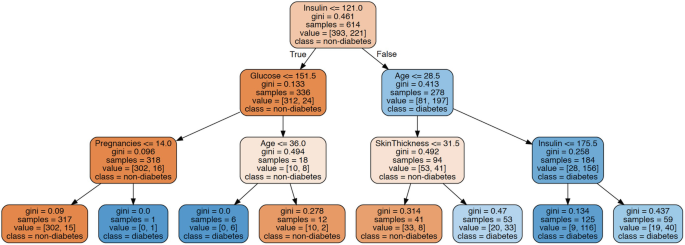

  

  Decision Tree which is constrained to be three-level deep for the diabetes classification data

• As discussed, Gini score quantifies the purity of the node/leaf. A Gini score greater than zero implies that samples contained within that node belong to different classes. A Gini score of zero means that the node is pure, i.e., that node consists of representatives from only one class.

• Starting from the root node and traversing all the way to leaves, various human-interpretable rules can be derived. For example, Insulin ≤ 121.0ANDGlucose ≤ 151.5ANDPregnancies ≤ 14.0 is a predictor of non-diabetes with 302 samples and resulting in only 15 errors (diabetes).

• The decreasing Gini score at each node level shows why the node/leaf is getting purer, and the rules are generalized.

Explainable properties of CART are shown in Table 3.8.

Table 3.8 Explainable properties of CART

3.7.9 Rule Induction

Rule induction is another popular traditional white-box technique in machine learning. Instead of starting from decision trees and converting them into rules, rule induction induces rules in the form of “IF <conditions >then class.” As compared to decision trees, which use the “divide-and-conquer” strategy, rule induction works through the “separate-and-conquer” approach [BGH89, CG91, Mic83a].

The general algorithm is to learn “one rule” at a time that “covers” positive instances in the dataset, remove those, and iteratively learn new rules until all positives are covered. The technique is also known as “sequential covering.” Creating conditions for the “if” requires searching for feature-value combinations, and there are various search techniques such as exhaustive, greedy/heuristic-based such as beam search, genetic algorithms, etc. There are multiple metrics to evaluate while learning a rule, such as accuracy, weighted accuracy, precision, information gain, etc., thus resulting in many variants. Similarly, there are multiple ways to arrange the rules during the inference. One can order the rules in the same way that it learned, metrics-based (accuracy, etc.), or some strategy-based for unordered execution. Often, the rules, like decision trees, can overfit to the training data. Two general approaches to overcome overfitting are pre-pruning and post-pruning. In pre-pruning, the rules stop at a certain point before it classifies or covers the instances perfectly, thus introducing some errors. In post-pruning, the training data is further split into growing and pruning sets; rule learning happens on the growing set to overfit the data, and post-pruning prunes these rules and uses the pruning set as validation data.

The most popular rule induction algorithms used in many applications are CN2, M5Rules, and RIPPER [CN89, Coh95a, HHF99, Qui92]. We use the Orange library to model the diabetes dataset as shown in Fig. 3.28.

Fig. 3.28

Building CN2 rule induction using orange

Interpretation of CN2 Rules:

• CN2 output has a sequence of ordered rules. Each rule has an “If condition” part that has at minimum a triplet of feature, operator, and value, e.g., Glucose ≥ 158.0 or combinations of these triplets with “AND” operator, e.g., Glucose ≥ 158.0 AND SkinThickness ≥ 44.0.

• The rule also has the “THEN clause” that implies a class that the rule captures (positive or negative in binary classification) and the distribution of positives and negatives the rule captures.

• The negatives captured in the positive class are the false positives, and the positives captured in the negative class are the false negatives.

Observations:

• We constrained the CN2 algorithm to have maximum rule length of 5, i.e., not more than 5 feature-operator-value are in conjunction. We also constrain that a rule should at least capture 8 examples in the dataset. These hyperparameters were manually searched. The maximum rule length and minimum examples act as a regularizer and prevent overfitting.

• Figure 3.29 shows only the rules for the positive class, i.e., outcome = 1.

  Fig. 3.29

  

  Rules covering positive class in the diabetes dataset

• The CN2 Rule Induction algorithm generates 55 rules on the dataset, 22 for the positive class.

• Only 4 rules out of 22 generate false positives, showing a good recall on the training data.

• There are interesting domain-specific rules such as “Age ≤ 31 AND Glucose ≥ 155.0” and “Age ≤ 29 AND Glucose ≥ 171.0”which captures young population with high glucose.

• There are some interesting ranges of certain features and relationship with other features captured such as the rule “Insulin ≥ 70 AND Insulin ≤ 193.0 AND BMI ≥ 34.2 AND BloodPressure ≥ 60.0” with 14 true positives with no false positives.

Explainable properties of CN2 rules are shown in Table 3.9.

Table 3.9 Explainable properties of CN2 Rules

References

D.A. Belsley, et al., Regression Diagnostics: Identifying Influential Data and Sources of Collinearity. Wiley Series in Probability and Statistics - Applied Probability and Statistics Section Series (Wiley, Hoboken, 1980). ISBN: 9780471058564
L.B. Booker, D.E. Goldberg, J.H. Holland, Classifier systems and genetic algorithms. Artif. Intell. 40(1–3), 235–282 (1989)
A.P. Bradley, The use of the area under the ROC curve in the evaluation of machine learning algorithms. Pattern Recog. 30(7), 1145–1159 (1997)
L. Breiman et al., Classification and Regression Trees (Wadsworth and Brooks, Monterey, 1984)
G.C. Cawley, N.L.C. Talbot, On over-fitting in model selection and subsequent selection bias in performance evaluation. J. Mach. Learn. Res. 11, 2079–2107 (2010)
C.-C. Chan, J.W. Grzymala-Busse, On the attribute redundancy and the learning programs ID3, PRISM, and LEM2. Department of Computer Science, University of Kansas. Technical Report TR-91- 14, December 1991 (1991)
J. Chen et al., The Use of Decision Threshold Adjustment in Classification for cancer Prediction (National Center for Toxicological Research Food and Drug Administration, Jefferson, Arkansas, 2015). http://www.ams.sunysb.edu/~hahn/psfile/papthres.pdf
P. Clark, T. Niblett, The CN2 induction algorithm. Mach. Learn. 3(4), 261–283 (1989)
W.W. Cohen, Fast effective rule induction, in Machine Learning Proceedings 1995 (Elsevier, Amsterdam, 1995), pp. 115–123
R.D. Cook, Cook’s distance, in International Encyclopedia of Statistical Science (Springer, Berlin, 2011), pp. 301–302. ISBN: 978-3-642-04898-2
G.F. Cooper, C. Yoo, Causal discovery from a mixture of experimental and observational data, in UAI ’99: Proceedings of the Fifteenth Annual Conference on Uncertainty in Artificial Intelligence (Morgan Kaufmann, Burlington, 1995), pp. 116–125
J. Davis, M. Goadrich, The relationship between precision- recall and ROC curves, in ICML ’06: Proceedings of the 23rd International Conference on Machine Learning (Association for Computing Machinery, New York, 2006), pp. 233–240. ISBN: 1-59593-383-2
N. Friedman, D. Geiger, M. Goldszmidt, Bayesian network classifiers. Mach. Learn. 29(2–3), 131–163 (1997)
S. Garcia, et al., A survey of discretization techniques: Taxonomy and empirical analysis in supervised learning. IEEE Trans. Knowl. Data Eng. 25(4), 734–750 (2012)
T. Gneiting, P. Vogel, Receiver Operating Characteristic (ROC) Curves (2018). arXiv: 1809.04808 [stat.ME]
Y. Guo, G. Bai, Y. Hu, Using bayes network for prediction of type-2 diabetes, in 2012 International Conference for Internet Technology and Secured Transactions (IEEE, Piscataway, 2012), pp. 471– 472
T.J. Hastie, R.J. Tibshirani, Generalized Additive Models, vol. 43 (CRC Press, Boca Raton, 1990)
T. Hastie, R. Tibshirani, Generalized additive models: some applications. J. Amer. Statist. Assoc. 82(398), 371–386 (1987)
T. Hastie, R. Tibshirani, J. Friedman, The Elements of Statistical Learning. Springer Series in Statistics, Chap. 15 (Springer, Berlin, 2009)
A.E. Hoerl, R.W. Kennard, Ridge regression: biased estimation for nonorthogonal problems. Technometrics 42(1), 80–86 (2000). ISSN: 0040-1706. http://doi.org/10.2307/1271436
M. Hollander, D.A. Wolfe, Nonparametric Statistical Methods (Wiley, New York, 1973)
G. Holmes, M. Hall, E. Frank, Generating rule sets from model trees, in Twelfth Australian Joint Conference on Artificial Intelligence (Springer, Berlin, 1999), pp. 1–12
J.F. Kenney, E.S. Keeping, Mathematics of Statistics. (van Nostrand, Princeton, 1962), pp. 252–285
D. Koller, N. Friedman, Probabilistic Graphical Models: Principles and Techniques (MIT Press, Cambridge, 2009)
P. McCullagh, J.A. Nelder, Generalized Linear Models. Chapman and Hall/CRC Monographs on Statistics and Ap- plied Probability Series, 2nd edn. (Chapman & Hall, London, 1989). ISBN: 9780412317606. http://books.google.com/books?id=h9kFH2%5C_FfBkC
R.S. Michalski, A theory and methodology of inductive learning, in Machine Learning (Elsevier, Amsterdam, 1983), pp. 83–134
J. Pearl, Probabilistic Reasoning in Intelligent Systems: Networks of Plausible Inference (Morgan Kaufmann, Burlington, 1988)
C. Perlich, Learning curves in machine learning, in Encyclopedia of Machine Learning (Springer US, Berlin, 2010). ISBN: 978-0-387-30164-8
F. Provost, Machine Learning from Imbalanced Data Sets 101 (Technical Report WS-00-05, AAAI, Menlo Park, CA, 2000), pp. 1–3
R.J. Quinlan, Learning with continuous classes, in 5th Australian Joint Conference on Artificial Intelligence (World Scientific, Singapore, 1992), pp. 343–348
S. Raschka, Model Evaluation, Model Selection, and Algorithm Selection in Machine Learning (2020). arXiv: 1811.12808 [cs.LG]
S.J. Russell, P. Norvig, Artificial Intelligence: A Modern Approach, 3rd edn. (Pearson, London, 2009)
S.H. Walker, D.B. Duncan, Estimation of the probability of an event as a function of several independent variables. Biometrika 54, 167–179 (1967)
H. Zou, T. Hastie, Regularization and variable selection via the elastic net. J. Roy. Statist. Soc. Ser. B (Statist. Methodol.) 67(2), 301–320 (2003)
Author information
Authors and Affiliations
Rights and permissions
Copyright information
© 2021 The Author(s), under exclusive license to Springer Nature Switzerland AG
About this chapter
Cite this chapter
Kamath, U., Liu, J. (2021). Model Visualization Techniques and Traditional Interpretable Algorithms. In: Explainable Artificial Intelligence: An Introduction to Interpretable Machine Learning. Springer, Cham. https://doi.org/10.1007/978-3-030-83356-5_3
Download citation
DOI: https://doi.org/10.1007/978-3-030-83356-5_3
Published:
Publisher Name: Springer, Cham
Print ISBN: 978-3-030-83355-8
Online ISBN: 978-3-030-83356-5
eBook Packages: Computer ScienceComputer Science (R0)