Forecasting of Retail Produce Sales Based on XGBoost Algorithm

Abstract

Sales forecasting of vegetables and fruits imposes a challenging task for the retailers because the demand for them varies depending on several factors, such as temperature, season, holiday. Poor sales forecasting can cause too much cost for retailers since these products are unusable after deterioration. Also, people tend to consume these products freshly. This research aims to compare the forecasting performance of traditional statistical and new machine learning methods. We apply seasonal ARIMA to forecast daily sales of fruits and vegetables as a traditional method. As a machine learning algorithm, we apply LSTM and XGBoost algorithms. The results indicate that the XGBoost algorithm gives more accurate results than the other two methods.

Introduction

Determining the stock levels of perishable products is more complicated than nonperishable products due to their short shelf life and customer behavior toward them [2, 26]. Therefore, it is necessary to develop different stock policies (van Donselaar 2006) and supply chain (SC) strategies [7, 28] for these foods. Fruits and vegetables, which are largely studied in this study, are classified as perishable foods with particular storage characteristics. Managing the fruits and vegetables supply chain is complex and difficult because of their fluctuating demand pattern. Several factors, such as weather conditions (Agnew and Tornes 1995), price changes [15], seasonality [19], are identified as the causes of variation in the demand of these foods. For Arunraj and Ahrens [5], factors can be classified as controllable factors, partially controllable factors, or uncontrollable factors. The authors state that the first includes price and product characteristics, the second includes substitution and cannibalization, and third includes events, weather, seasonality, and the number of customers. If organizations do not take into account these factors in stock management, they may suffer financial losses due to the waste of food and loss of customers. Optimized replenishment of these foods at the retail level is key to reducing the waste of these foods and increasing the efficiency of the fruits and vegetables supply chain. Optimal replenishment orders depend upon the sales forecasting [22]. Sales forecasting do not only enable retail managers to cope with stochastic demand, but also helps to maintain a competitive advantage in SC management.

Although the replenishment process for these foods usually performed manually by managers based on experience and the point of system (POS system) the necessity of analytical techniques has been understood lately, and more recent research has occurred in the demand forecasting of the perishable foods based on traditional statistical methods (causal models, time series and econometric methods) and machine learning (ML) methods. Sankaran [23] uses the Seasonal ARIMA model to forecast the daily demand for onion at a wholesale market and conclude that forecasting performance is satisfactory with an erratic demand. Raju et al. [21] investigate the factors causing the stochastic demand for perishable foods and examines the forecasting performance of linear and nonlinear forecasting methods. It concludes that temperature is the predominant factor that influences the demand, and nonlinear methods generate more accurate results than linear methods. Yang and Sutrisno (2018) bring a new perspective to forecast the demand for the bakery at franchise stores. The idea is to use sales occurring in the early morning hour to forecast the sales of the rest of the day. They also compare the forecasting performance of Feed Forward Neural Network (FFNN) and Regression analysis. They conclude that this approach is very promising to generate online-forecasting, and FFNN gives better results than regression analysis. Sridama and Siribut [24] propose a decision support system for demand forecasting of perishable foods to improve the inventory management of these foods. They analyze the forecasting performance of the following time series methods: Single exponential smoothing, Adaptive-response-rate single exponential smoothing, and Holt’s two parameters linear exponential smoothing. They conclude that the Single exponential smoothing method gives better results than others. Huber and Stuckenschmidt (2017) propose a decision support system (DSS) based on the hierarchical clustering approach to obtain demand forecasts of perishable food at different organizational levels. They implemented the proposed DSS in the bakery chain of a company. The authors use multivariate ARIMA as a forecasting method. They conclude that the proposed approach gives acceptable results to increase the efficiency of the supply chain, and also decreases the computational time. The approach enables us to develop replenishment strategies based on product categories exhibiting similar demand patterns. Yang and Hu (2008) apply an ARIMA model to forecast the demand for cabbage.

Chen and Ou [13] propose an extended neural network model to forecast the daily demand for milk in a convenience store, and they compare the proposed model with an ARIMA model. The results indicate that the proposed model generates better results than the ARIMA model. Du et al. [14] develop an algorithm based on the Support vector machine and fuzzy theory to forecast the demand for perishable farm foods. They conclude that the proposed algorithm gives more promising results than radial basis function neural networks.

Although time series forecasting is generally superior to judgemental and econometric forecasting techniques for forecasting retail sales [16], it still lacks capturing the sudden changes in demand due to characterized nature of perishable foods. The forecasting performance of these methods may be improved by using hybridized versions of them [5]. Chen and Ou [10] propose a model which combines gray relational analysis and multilayer functional network model to forecast the sales of perishable food in a convenience store.

While these hybrid methods have provided considerable improvement in forecasting accuracy, much of it was not focusing especially on forecasting the fruits and vegetable sales at the retail levels. Furthermore, the forecasting accuracy is still required to improve by applying new algorithms. To improve the forecasting accuracy, this study focuses on the application of a gradient boosting ML algorithm, Extreme Gradient Boosting algorithm (XGBoost) due to its capabilities to handle the sparse data (Chen and Guestrin 2016), and computational efficiency, and it is popularity in ML competitions (Chen and He 2015). The results of the model are encouraging and show that XGBoost outperforms than classical SARIMA and LSTM models.

The rest of the paper is organized as follows: Sect. 2 outlines our method, which is used in this study and presents the description of data. Section 3 discusses the results of the performance of applied methods. Finally, Sect. 4 gives the conclusion and future research of the study.

Methodology

Description of Data

This study uses daily sales data of vegetables and fruits from a supermarket in Istanbul, Turkey, as a case study from January 2014 to December 2017. It would be more appropriate to conduct the forecasting on the product level due to the product-specific nature of demand pattern. Unfortunately, aggregate daily sales of vegetables and fruits are considered due to a lack of sales data on the product level. Figure 1 shows the daily sales data of vegetables and fruits in the time series plot. This time series plot shows that there is no obvious trend in data. There is an increasing trend in the sales of vegetables and fruits on some dates, such as the last week of the year. This cyclic pattern is repeated every year. This weekly or seasonal variation may be attributable to some causes such as the impact of weather or holidays.

Fig. 1

The annual sales of vegetables and fruits (green indicates vegetables, red indicates fruits)

Time Series

A time series is a sequential set of observations measured at successive times [8]. There are four key components of time series data, which should be analyzed before applying an algorithm: (1) Trend, (2) Seasonality, (3) Cyclical, and (4) Irregularity. Trend describes the general direction of observations over a long time. Seasonality explains the variation in the observations over a period of one year, usually caused by weather conditions, holidays, vacations, etc. Cyclical refers to the nonperiodic variations caused by circumstances, which occur in a repeating pattern. The duration of these variations lasts several years. Irregularity refers to the random variations in observations caused by unforeseeable reasons, such as earthquakes, floods, epidemic diseases, etc. Expectedly, these variations do not have a particular pattern. Time series plots may reveal these patterns or a combination of these patterns [3].

One of the most critical behaviors of a time series is stationarity. The stationarity of a time series data indicates its statistical behavior in time. When a time series exhibits this property, the statistical behavior of that series does not change in time. This means that it has a constant probability distribution. A time-series data must have this property because nonstationary data cannot be forecasted due to its unstable nature. If a time series data does not have stationarity behavior, it should be converted to a stationary form before performing any forecasting. There are two options to check the stationarity of a time series data: (1) Rolling statistics: plot the rolling average (moving average) and see how it varies with time, (2) ADCF (Augmented Dickey-Fuller Test) provides a formal statistical test to detect the stationarity property. The null hypothesis claims that the time series is nonstationary.

Seasonal ARIMA (SARIMA) Model

ARIMA stands for the autoregressive moving average, and it has three parameters: (p, d, q). AR component is referred to the use of past values in the regression equation for the series Y. The parameter p indicates the number of lags used in the model. MA component represents the error of the model as a combination of previous error terms. The parameter q specifies the number of terms to include in the model. The parameter d represents the degree of differencing in the integrated component. Differencing a series involves simply subtracting its current and previous values d times. It is used to stabilize the data to satisfy the stationarity assumption [9]. SARIMA (Seasonal ARIMA) is an extension to ARIMA, which allows the direct modeling of seasonal behavior of data. SARIMA model is represented by the following notation: ARIMA (p, d, q) (P, D, Q)_s. The lower-case (p, d, q) is the same as the nonseasonal ARIMA model. The upper-case (P, D, Q) represents the seasonal parameters of the model. The subscripted letter s indicates the length of the period in each season. For example, in monthly data, s = 12. Let d and D are nonnegative integers. A SARIMA model general form is given in Eq. (1)

$$\emptyset_{P} \left( B \right)\Phi _{P} \left( {B^{s} } \right)Y_{t} =\uptheta _{q} \left( B \right)\Theta _{Q} \left( {B^{S} } \right)\varepsilon_{t}$$

(1)

$$\emptyset_{P} \left( B \right) = 1 - \phi_{1} B - \phi_{2} B^{2} - \ldots - \phi_{P} B^{P}$$

(2)

$$\Phi _{P} \left( {B^{S} } \right) = 1 -\Phi _{S} B^{S} -\Phi _{2S} B^{2S} - \ldots -\Phi _{PS} B^{PS}$$

(3)

$$\uptheta _{q} \left( B \right) = 1 -\uptheta _{1} B -\uptheta _{2} B^{2} - \ldots -\uptheta _{q} B^{q}$$

(4)

$$\Theta _{Q} \left( {B^{S} } \right) = 1 -\Theta _{S} \left( {B^{S} } \right) -\Theta _{2S} \left( {B^{2S} } \right) - \ldots -\Theta _{QS} \left( {B^{QS} } \right)$$

(5)

where {X_t} is the original series; ${\text{Y}}_{{\text{t}}} = (1 - {\text{B}})^{{\text{d}}} \left( {1 - {\text{B}}^{{\text{s}}} } \right)^{{\text{D}}} {\text{X}}_{{\text{t}}}$ is differenced series to eliminate seasonality component; B is the lag operator; $\emptyset \left( B \right)$ and ${\uptheta }\left( B \right)$ are polynomials of order p and q, respectively; $\Phi \left( {B^{S} } \right)$ and $\Theta \left( {B^{S} } \right)$ are polynomial in B of degrees P and Q respectively; p is the order of nonseasonal autoregression; d is the number of regular differences; q is the order of nonseasonal moving average; P is the order of seasonal autoregression; D is the number of seasonal differences; Q is the order of seasonal moving average; and S is the length of the season [9]. The steps of the model are explained in the section of the application of the SARIMA model.

Long Short-Term Memory (LSTM)

Feedforward neural networks are not suitable for sequential data due to their fixed-size input/output. Therefore, they cannot be used to model memory. On the other hand, recurrent neural networks (RNN) are designed for capturing information from time-series data. In an RNN, thanks to the recurrence relation, each state is dependent on all previous computations. In theory, RNNs are capable of remembering information for long sequential data. However, in practice, this is not feasible due to the vanishing/exploding gradient problem. A similar problem is observed in deep feedforward networks. The source of this problem is the nature of RNN, which is using the same weight matrix to compute all the state updates. Even though the theory states that RNN can be used to learn long-term dependencies, due to vanishing/exploding gradient problems, they only seem to limit themselves to learn short-term dependencies.

LSTM solves the vanishing gradient problem and gives more accurate results compared to regular RNN. LSTM consists of three gates (forget, input, and output) and one cell state [17]. These are defined as follows:

$$f_{t} = \sigma \left( {w_{f} h_{t - 1} + w_{f} x_{t} } \right)$$

(6)

$$i_{t} = \sigma \left( {w_{i} h_{t - 1} + w_{i} x_{t} } \right)$$

(7)

$$o_{t} = \sigma (w_{o} h_{t - 1} + w_{o} x_{t)}$$

(8)

$$\widetilde{{c_{t} }} = \tanh \left( {w_{c} h_{t - 1} + w_{c} x_{t} } \right)$$

(9)

$$c_{t} = \left( {i_{t} *\widetilde{{c_{t} }}} \right) + \left( {f_{t} *c_{t - 1} } \right)$$

(10)

$$h_{t} = o_{t} *\tanh \left( {c_{t} } \right)$$

(11)

Here $f, i, o$ are forget, input and output gates respectively, c is cell state, h is a hidden state and x is the input. The complete structure of the LSTM is illustrated in Fig. 2.

Fig. 2

LSTM structure

LSTM can hold a combination of different information blocks at each time step. The main advantage of LSTM comes from the cell state. Cell state provides the possibility of explicitly information writing or removing. This cell state can only be altered by the gates which are responsible for letting the information pass through.

From previous studies, we know that the convolution operation works well to extract features as local input patches. This allows modular and efficient data representations. In our forecasting problem, we accept the time as a spatial dimension and process the data by applying 1D convolution operations to extract subsequences from the sequence. This allows us to recognize local patterns since the same transformation is applied to every patch. However, it is not possible to get reasonable results in forecasting problems just by using convolution operation. Since the convolution operation processes the input patches independently, it is not sensitive to the order of the timestep, unlike LSTM. One way to use the advantageous feature of convolution is to use it as a preprocessing step before LSTM. Figure 3 illustrates our data processing step combined with LSTM.

Fig. 3

Data feed processing

XGBoost (Extreme Gradient Boosting)

XGBoost is a scalable end-to-end novel machine learning algorithm based on tree learning gradient boosting that can handle sparse data in a highly efficient way. The mathematical formulation of the model is described by Chen and Guestrin (2016) as follows: Eq. (12) describes the objective function (also called loss function) which should be minimized at iteration t where $\hat{y}_{i}^{\left( t \right)}$ indicates the prediction of ith instance at ith iteration; $\Omega \left( {f_{t} } \right)$ describes the regularization term, which helps to model to avoid over-fitting results.

$${\mathcal{L}}^{\left( t \right)} = \mathop \sum \limits_{i = 1}^{n} l\left( {y_{i} , \hat{y}_{i}^{{\left( {t - 1} \right)}} + f_{t} \left( {x_{i} } \right)} \right) +\Omega \left( {f_{t} } \right)$$

(12)

At each iteration, a new function $f_{t}$ is added, which provides the best improvement for the model. It is not possible to solve Eq. (12) by using traditional optimization methods. So second-order Taylor approximation is used to get a solvable form by traditional methods and Eq. (13) is obtained. Where $g_{i} = \partial_{{\hat{y}^{{\left( {t - 1} \right)}} }} l\left( {y_{i} , \hat{y}^{{\left( {t - 1} \right)}} } \right)$ and $h_{i} = \partial^{2}_{{\hat{y}^{{\left( {t - 1} \right)}} }} l\left( {y_{i} , \hat{y}^{{\left( {t - 1} \right)}} } \right)$ are first and second-order terms respectively at iteration t. When we remove the constant term in Eq. (13), we obtain Eq. (14).

$${\mathcal{L}}^{\left( t \right)} = \mathop \sum \limits_{i = 1}^{n} \left[ {l(y_{i} , \hat{y}_{i}^{{\left( {t - 1} \right)}} + g_{i} f_{t} \left( {x_{i} } \right) + \frac{1}{2}h_{i} f_{t}^{2} \left( {x_{i} } \right)} \right] +\Omega \left( {f_{t} } \right)$$

(13)

$$\widetilde{{\mathcal{L}}}^{\left( t \right)} = \mathop \sum \limits_{i = 1}^{n} \left[ {g_{i} f_{t} \left( {x_{i} } \right) + \frac{1}{2}h_{i} f_{t}^{2} \left( {x_{i} } \right)} \right] +\Omega \left( {f_{t} } \right)$$

(14)

If regularization term $\Omega \left( {f_{t} } \right)$ is replaced by $\gamma T + \frac{1}{2}\lambda \mathop \sum \limits_{j = 1}^{T} w_{j}^{2}$, then objective function takes its final form as follows:

$$\begin{aligned} \widetilde{{\mathcal{L}}}^{\left( t \right)} & = \mathop \sum \limits_{i = 1}^{n} \left[ {g_{i} f_{t} \left( {x_{i} } \right) + \frac{1}{2}h_{i} f_{t}^{2} \left( {x_{i} } \right)} \right] + \gamma T + \frac{1}{2}\lambda \mathop \sum \limits_{j = 1}^{T} w_{j}^{2} \\ & = \mathop \sum \limits_{j = 1}^{T} \left[ {\left( {\mathop \sum \limits_{{i \in I_{j} }} g_{i} } \right)w_{j} + \frac{1}{2}\left( {\mathop \sum \limits_{{i \in I_{j} }} h_{i} + \lambda } \right)w_{j}^{2} } \right] + \gamma T \\ \end{aligned}$$

(15)

The optimal value of weights $w_{j}$ at leaf j is obtained by using Eq. (16) and the optimal value is calculated by Eq. (17). This equation can be understood as a scoring function for a tree structure q. This score is similar to the impurity score for evaluating decision trees.

$$w_{j}^{*} = - \frac{{\mathop \sum \nolimits_{{i \in I_{j} }} g_{i} }}{{\mathop \sum \nolimits_{{i \in I_{j} }} h_{i} + \lambda }}$$

(16)

$$\widetilde{{\mathcal{L}}}^{\left( t \right)} \left( q \right) = - \frac{1}{2}\mathop \sum \limits_{j = 1}^{T} \frac{{\mathop \sum \nolimits_{{i \in I_{j} }} g_{i} }}{{\mathop \sum \nolimits_{{i \in I_{j} }} h_{i} + \lambda }} + \gamma T$$

(17)

It is a real challenge to enumerate all possible trees. The authors propose Eq. (18) to calculate the score of each tree structure for evaluating each one to select the best split where $I_{L}$ and $I_{R}$ denotes the instances set of left and right nodes after the split;

$I = I_{L} \cup I_{R}$.

$${\mathcal{L}}_{split} = \frac{1}{2}\left[ {\frac{{\left( {\mathop \sum \nolimits_{{i \in I_{L} }} g_{i} } \right)^{2} }}{{\mathop \sum \nolimits_{{i \in I_{L} }} h_{i} + \lambda }} + \frac{{\left( {\mathop \sum \nolimits_{{i \in I_{R} }} g_{i} } \right)^{2} }}{{\mathop \sum \nolimits_{{i \in I_{R} }} h_{i} + \lambda }} - \frac{{\mathop \sum \nolimits_{i \in I} g_{i} }}{{\mathop \sum \nolimits_{{i \in I_{I} }} h_{i} + \lambda }}} \right]$$

(18)

Application of SARIMA Model

The steps involved in building a SARIMA model are as follows:

• 1. Identification of Model Parameters: the initial step of the SARIMA is to determine the values of parameters. The autocorrelation, partial autocorrelation, and Augmented Dickey-Fuller (ADF) test results for vegetables and fruits are shown in Fig. 4. The plots indicate that there is no regular or seasonal trend. ADF results also prove that both data satisfy stationarity property at 0.05. The best values of parameters should be identified. To determine the parameters of the model, Akaike’s Information Criterion (AIC) is commonly utilized. It is calculated as follows:

  $$AIC\left( p \right) = n\ln \left( \frac{RSS}{n} \right) + 2K$$

  (19)

  Fig. 4

  

  Seasonal and stationary analysis of fruits and vegetables respectively

where n is the number of observations, and RSS is the residual sums of squares. The parameters providing the minimum AIC value will be set as model parameters. Another approach for determining appropriate parameters of the model is to analyze (ACF) and (PACF) plots.

• 2. Estimation of Model Parameters: A grid search approach is employed for determining the best forecasting model in this study. ARIMA (p, d, q) (P, D, Q) m model requires six parameters: p, d, q, P, D, and Q. The value of m is set as 12 because used data are monthly with a period of 12. The AIC values of evaluated models are shown in Table 1. According to Table 1, SARIMA (1, 1, 1) × (1, 0, 1)12 shows the lowest AIC value. Thus, this model should be considered as the best forecasting model. According to Table 1, the AIC value of SARIMA (1, 1, 2) × (0, 0, 1)12 is the lowest.

  Table 1 AIC Values of SARIMA models

• 3. Diagnostic of Model: In this step, the statistical importance of the selected SARIMA model is determined. The statistical test results of the SARIMA (1, 1, 1) × (0, 0, 1, 1) model are shown in Table 2. The second column indicates the weight of the coefficients. Since all values of P > |z| are less than 0.05 (significance level), we can conclude that all coefficients are statistically significant.

  Table 2 Results of the diagnostics test of the SARIMA (1, 1, 2) × (0, 0, 1, 1) model

• 4. Forecasting: The model with estimated parameters is used to make forecasts. Data from January 2014 to December 2016 are used as a training set, and the remaining data is used as test data. We forecast the periods between January and December 2017 daily. Figure 5 shows the model forecast values and the actual value curve. Mean absolute percentage error (MAPE) on the test data set is 24.57 and 24.43% for fruits and vegetables respectively.

  Fig. 5

  

  Forecast value and actual value fitting curve

Application of LSTM Model

The algorithm is implemented in Python with the Pytorch library.

• 1. Model Parameters: Our network consists of 1 hidden layer with 9 neurons. The output activation function is linear. The input to the network is our 17 handcrafted features. Mean squared error loss is selected for loss calculation. A popular ADAM optimization algorithm was selected to optimize network weight values. Hyperparameters of the model and optimization algorithm are selected based on trial-and-error.

• 2. Data Processing: Total data split into two parts as follows: first three-year data as training and the last year as testing. The windows size of the 1D convolution operation was selected as 12. Before feeding the inputs into the network, additional scaling/normalization processes applied as in regular feedforward neural networks to make the learning step more stable.

• 3. Forecasting: Neural network trained for 2000 epochs. No regularization method was applied to the implementation.

Training loss for vegetable sales data is illustrated in Fig. 6. MAPE on test data is 24.6, which is inside an acceptable boundary compared to previous studies. Figure 8 shows the prediction of vegetable data. To forecast fruit data, the same LSTM network is retrained by using the same hyperparameters. Figures 7 and 8 show the results for fruit data. In this case, MAPE is 22.5.

Fig. 6

LSTM traning loss for vegetable

Fig. 7

LSTM traning loss for fruit

Fig. 8

Forecast value and actual value fitting curve for vegetable (top) and fruit (bottom)

Application of XGBoost (Extreme Gradient Boosting)

The algorithm is implemented in Python using open-source XGBoost libraries. An open-source framework provides a fast and easy implementation of the algorithm. The following steps are involved in the implementation of the algorithm.

• 1. Feature extraction and selection: We extract 17 features after reading the papers in the area and obtain the relative importance of these features, as shown in Fig. 9. The temperature and dollar rate are the most important features. The categorical variables are converted into the numerical form by using one-hot encoding.

  Fig. 9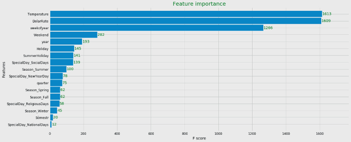

  

  Feature importance plot

• 2. Parameter Tuning: The XGBoost algorithm has too many parameters, and the values of these parameters highly affect the prediction performance of the model. So it is required to perform hyper-parameter tuning operation to obtain the more appropriate model. It is the most time-consuming part of the implementation of the algorithm. The custom grid search approach is used to find the parameter values. The booster parameters related to the learning task and model complexity are tuned by using the given values in Table 3. These values are determined based on the expert’s suggestions. Column 2 indicates the used values in the grid search process, and column 3 represents the best value of tuned parameters. Default values are used for the remaining parameters.

  Table 3 Hyper-parameter tuning values

• 3. Forecasting: After selecting the best model parameters, we can use the model to make forecasting. Figure 10 shows the model forecast values and the actual value curve. The forecasting results indicate that XGBoost can make better predictions than SARIMA and LSTM (see Table 4).

  Fig. 10

  

  Forecast value and actual value fitting curve

  Table 4 Performance comparison of forecasting methods based on MAPE

Summary and Outlook

In this study, we focused on the applicability of the XGBoost algorithm to forecast the daily sales of perishable foods. A specific focus of the study was directed toward two special perishable food categories: vegetables and fruits. The test cases were performed in the retail market. The results show that XGBoost yields better predictions compared to SARIMA and LSTM. The outcomes of this study can give several useful insights for managers, such as the development of stock policy, investments in SC.

Although we obtained meaningful results, some limitations and future research avenues may be emphasized. First, the advantage of using ML techniques highly depends on data availability. Since all factors are not included in the model due to a lack of data availability, we could not fully exploit the advantages of ML methods. Second, the controllable factors, such as product characteristic, promotions are not used in this study. With the availability of all these features, the most relevant features can be identified.

These limitations imply many possible extensions of this study in the future. For example, product-based or location-based estimation can be employed to understand the impact of these factors on sales. Besides, it is possible to investigate different ML algorithms, as well as new methods of combining these algorithms while considering the respective accuracy of each.

References

Aburto L, Weber R (2007) Improved supply chain management based on hybrid demand forecasts. Appl Soft Comput 7(1):136–144
Adebanjo D, Mann R (2000) Identifying problems in forecasting consumer demand in the fast-moving consumer goods sector. Benchmarking Int J
Adhikari R, Agrawal RK (2013) An introductory study on time series modeling and forecasting. arXiv preprint arXiv:1302.6613
Agnew MD, Thornes JE (1995) The weather sensitivity of the UK food retail and distribution industry. Meteorol Appl 2(2):137–147
Arunraj NS, Ahrens D (2015) A hybrid seasonal autoregressive integrated moving average and quantile regression for daily food sales forecasting. Int J Prod Econ 170:321–335
Ashagidigbi WM, Adebayo AS, Salau SA (2019) Analysis of the demand for fruits and vegetables among households in Nigeria. Sci Lett 7(2):45–51
Blackburn J, Scudder G (2009) Supply chain strategies for perishable products: the case of fresh produce. Prod Oper Manag 18(2):129–137
Brockwell PJ, Davis RA, Fienberg SE (1991) Time series: theory and methods: theory and methods. Springer Science & Business Media
Brockwell PJ, Davis RA (2016) Introduction to time series and forecasting. Springer
Chen FL, Ou TY (2009) Gray relation analysis and multilayer functional link network sales forecasting model for perishable food in convenience store. Exp Syst Appl 36(3):7054–7063
Chen T, He T (2015) Higgs boson discovery with boosted trees. In: NIPS 2014 workshop on high-energy physics and machine learning, pp 69–80
Chen T, Guestrin C (2016) Xgboost: a scalable tree boosting system. In Proceedings of the 22nd ACM SIGKDD international conference on knowledge discovery and data mining, pp 785–794
Chen FL, Ou TY (2008) A neural-network-based forecasting method for ordering perishable food in convenience stores. In: 2008 fourth international conference on natural computation, vol 2. IEEE, pp 250–254
Du XF, Leung SC, Zhang JL, Lai KK (2013) Demand forecasting of perishable farm products using support vector machine. Int J Syst Sci 44(3):556–567
Durham C, Eales J (2010) Demand elasticities for fresh fruit at the retail level. Appl Econ 42(11):1345–1354
Geurts MD, Kelly JP (1986) Forecasting retail sales using alternative models. Int J Forecast 2(3):261–272
Hochreiter S, Schmidhuber J (1997) Long short-term memory. Neural Comput 9(8):1735–1780
Huber J, Gossmann A, Stuckenschmidt H (2017) Cluster-based hierarchical demand forecasting for perishable goods. Expert Syst Appl 76:140–151
Locke E, Coronado GD, Thompson B, Kuniyuki A (2009) Seasonal variation in fruit and vegetable consumption in a rural agricultural community. J Am Diet Assoc 109(1):45–51
Paam P, Berretta R, Heydar M, Middleton RH, García-Flores R, Juliano P (2016) Planning models to optimize the agri-fresh food supply chain for loss minimization: a review. Ref Mod Food Sci 19–54
Raju Y, Kang PS, Moroz A, Clement R, Hopwell A, Duffy AP (2016) Investigating the demand for short-shelf-life food products for SME wholesalers
Reddy AS, Chakradhar P, Santosh T (2018) Demand forecasting and demand supply management of vegetables in India: a review and prospect. Int J Comput Technol 17(1):7170–7178
Sankaran S (2014) Demand forecasting of fresh vegetable product by seasonal ARIMA model. Int J Oper Res 20(3):315–330
Sridama P, Siribut C (2018) Decision support system for customer demand forecasting and inventory management of perishable goods. J Adv Manag Sci 6(1)
van Donselaar K, Van Woensel T, Broekmeulen RACM, Fransoo J (2006) Inventory control of perishables in supermarkets. Int J Prod Econ 104(2):462–472
Van Woensel T, Van Donselaar K, Broekmeulen R, Fransoo J (2007). Consumer responses to shelf out‐of‐stocks of perishable products. Int J Phys Distrib Logistics Manag
Yang CL, Sutrisno H (2018) Short-term sales forecast of perishable goods for franchise business. In 2018 10th international conference on knowledge and smart technology (KST). IEEE, pp 101–105
Yang S, Xiao Y, Kuo YH (2017) The supply chain design for perishable food with stochastic demand. Sustainability 9(7):1195
Yang HX, Hu J (2013) Forecast of fresh agricultural products demand based on the ARIMA model. Guangdong Agric Sci 11:52
Author information
Authors and Affiliations
Corresponding author
Editor information
Editors and Affiliations
Rights and permissions
Copyright information
© 2022 The Author(s), under exclusive license to Springer Nature Switzerland AG
About this paper
Cite this paper
Turgut, Y., Erdem, M. (2022). Forecasting of Retail Produce Sales Based on XGBoost Algorithm. In: Calisir, F. (eds) Industrial Engineering in the Internet-of-Things World. GJCIE 2020. Lecture Notes in Management and Industrial Engineering. Springer, Cham. https://doi.org/10.1007/978-3-030-76724-2_3
Download citation
DOI: https://doi.org/10.1007/978-3-030-76724-2_3
Published:
Publisher Name: Springer, Cham
Print ISBN: 978-3-030-76723-5
Online ISBN: 978-3-030-76724-2
eBook Packages: EngineeringEngineering (R0)