Cross-Domain Text Classification Based on BERT Model

Abstract

Diversity of structure and classification are difficulties for information security data. With the popularization of big data technology, cross-domain text classification becomes increasingly important for the information security domain. In this paper, we propose a new text classification structure based on the BERT model. Firstly, the BERT model is used to generate the text sentence vector, and then we construct the similarity matrix by calculating the cosine similarity. Finally, the k-means and mean-shift clustering are used to extract the data feature structure. Through this structure, clustering operations are performed on the benchmark data set and the actual problems. The text information can be classified, and the effective clustering results can be obtained. At the same time, clustering evaluation indicators are used to verify the performance of the model on these datasets. Experimental results demonstrate the effectiveness of the proposed structure in the two indexes Silhouette coefficient and Calinski-Harabaz.

1 Introduction

Information security is related to the survival and core interests of individuals, enterprises and even a country. The issue of information security is without worry, and national security and social stability are also guaranteed. An important aspect of information security technology is the efficient processing and classification of the existing massive information. After sorting out the data, it is convenient for managers to search and check regularly. The traditional text classification method, which usually takes words as the basic unit of text, is not only easy to cause the lack of semantic information, but also easy to lead to the high dimension and sparsity of text features. At present, the application of text classification technology is mostly machine learning. This method usually extracts TF-IDF (Term Frequency – Inverse Document Frequency, word frequency, inverse document frequency) or word bag features, and then trains LR (Logistic Regression) model. There are many models, such as Bayes, SVM (Support Vector Machine), etc. However, the generalization ability of text classifiers based on traditional methods tends to decrease when processing text data with diverse features. In recent years, deep learning technology has developed rapidly and has been applied in various fields with remarkable results. Deep learning has been widely used with its unique network structure, which can improve the effect of text preprocessing and solve the current problems of text classification.

Text classification [1] is a basic task in natural language processing and the most important step to solve the problem of text information overload, which can sort out and classify the existing massive text resources. The processing of text classification can be divided into text preprocessing, text feature extraction, classification model construction and so on. Classic text classification algorithms such as NB (Naïve Bayes), KNN (K-Nearest Neighbor), DTree (Decision Tree), AAC (Arithmetical Average Centroid), SVM (Support Vector Machine), etc. Text classification technology has an early origin and has experienced a development process from the expert system to machine learning and then to deep learning. The development of deep learning improves the high dimension and sparsity of traditional machine learning in text classification, which leads to more effective text representation methods. After Bengioetal (2003) proposed the forward Neural Network (feed-forward neural network, FNN) language model, its lexical vector measures the semantic correlation between words. In 2013, Mikolov proposed the Word2vec framework, which mainly uses the deep learning method to map words to low-dimensional real vector space, and captures semantic information of words by calculating the distance between word vectors. The deep learning-based text classification method uses lexical vectors to express the semantic meaning of words, and then obtains the semantic representation of text through semantic combination. The methods of a semantic combination of neural network mainly include convolutional neural network, cyclic neural network and attention mechanism, etc. These methods rise from semantic representation of words to semantic representation of text through different combination methods.

The BERT [2] (Bidirectional Encoder Representations from Transformers) model is the language presentation model released by Google in October 2018, and the replacement of the Word2Vec model has become a major breakthrough in NLP (Natural Language Processing) technology. BERT model in the top level machine reading comprehension test SQuAD1.1 showed remarkable achievements: two indexes are better than others, and it also makes the best grades in 11 different NLP tests, including pushing GLUE benchmark to 80.4% absolute improvement (7.6%), MultiNLI accuracy reached 86.7% (absolute improvement rate 5.6%). BERT model is actually a language encoder, which can transform the input sentence or paragraph into feature vectors. Word embedding is a way to map words to Numbers, but a simple real number contains too little information, generally we map to a numerical vector. In the process of natural language processing, it is necessary to retain some abstract features of the language itself, such as semantics and syntax. Throughout the development history of NLP, many revolutionary achievements are the development achievements of word embedding, such as Word2Vec, ELMo and BERT, which have well preserved the features of natural language in the transformation process.

This paper uses the BERT model in the process of generating word vectors, and then calculates the cosine similarity to generate the similarity matrix. In order to solve the problem of massive information management and improve the efficiency of managers, we have designed a set of research plans. First, we extract the information in the dataset and combine the BERT model to complete the construction of the text word vector, and then create the text similarity matrix. On the premise of ensuring accuracy, reduce the time loss in the community discovery process, and then perform clustering operations through k-means and mean-shift, and finally achieve the purpose of classifying papers.

2 Related Work

2.1 BERT Model

BERT [3] is a language representation model based on deep learning. The emergence of BERT technology has changed the relationship between pre-trained word vectors and downstream specific tasks. The word vector model is an NLP tool that transforms abstract text formats into vectors that can be used to perform mathematical computations on which NLP’s task is to operate. In fact, NLP technology can be divided into two main aspects: training text data to generate word vectors and operating these word vectors in the downstream model. At present, the technology to generate word vectors mainly includes word2VEc, ELMo, BERT and other models. The core module of BERT model is transformer, and the core of transformer is the attention mechanism. The attention mechanism draws lessons from human visual attention, which enables the neural network to focus on a part of the input, that is, it can distinguish the influence of different parts of the input on the output. BERT’s network architecture uses a multi-tier Transformer structure, which abandons the traditional RNN and CNN. The transformer is an Encoder-Decoder structure, which consists of several encoders and decoders stacked.

BERT Model Input

As shown in Fig. 1 below, BERT’s input adds “CLS” at the beginning of the first sentence as the beginning of the text, and “SEP” as the end.

Token Embeddings: To represent the word vector, each word is converted into a vector by establishing a word-to-word scale, which is used as the input representation of the model.

Segment Embeddings: This part is used to distinguish two sentences, because the pre-training needs to do the task of classifying two sentences.

Position Embeddings: This part is obtained through model training.

Fig. 1.

BERT model input.

BERT Model Pre-training Tasks

• I. Masked Language Model (MLM)

  In order to train in-depth both transformer representation, BERT [4] model adopts a simple approach: That is, on the model input text, the input words are randomly screened, and then the rest of the words are used to predict which part of the input is screened. For the masked text, a special symbol [MASK] is used 80% of the cases, a random word is used in 10% of the cases, and the original word is left unchanged in 10% of the cases. After this operation, the model does not know whether the words at the corresponding position are correct or not when predicting a word, which makes the model have to rely more on the context information to predict the word, and at the same time, the model has a certain ability to correct errors.

• II. Next Sentence Prediction

  The work of the Next Sentence Prediction is as follows: In any two sentences of a given text, determine whether the second sentence follows the first sentence in the original dataset. In other words, when inputting sentences A and B, B is 50% likely to be the next sentence of A, and 50% may be from anywhere in the text. Consider only two sentences and decide if they are the preceding and following sentences in an article. In the actual pre-training process, 50% correct sentence pairs and 50% wrong sentence pairs are randomly selected from the text corpus for training. Combined with the Masked LM task, the model can more accurately describe the semantic information of the sentence and even the text level.

The BERT [5] model performs joint training on the Masked LM task and the Next Sentence Prediction task, so that the vector representation of each word output by the model can describe the overall semantic information of the input text (single sentence or sentence pair) as comprehensively and accurately as possible. Provide better initial values of model parameters for subsequent fine-tuning tasks.

2.2 Matrix Preprocessing

Given graph H = (K, L), K = {${k}_{1},{k}_{2},\dots ,{k}_{n}$}. K represents the node set in the graph, and L represents the edge set in the graph. N(u) is the set of neighbor nodes of node u. Suppose matrix A = ${[{a}_{ij}]}_{n\times n}$ is the adjacency matrix of graph H, and the corresponding elements of the matrix indicate whether there is an edge between two points in graph H.

For example, ${a}_{ij}$ is 1 to indicate that there is an edge between ${k}_{i}$ and ${k}_{j}$ in graph H. If ${a}_{ij}$ is 0, it means two points. There is no edge in between ${k}_{i}$ and ${k}_{j}$ in graph H.

Similarity matrix: For a network graph H = (K, L), the similarity matrix S = ${[{s}_{ij}]}_{n\times n}$ is calculated through the similarity of nodes between two points in the graph H. The elements in the matrix are the similarity between two nodes.

Similarity calculation-cosine similarity [6]: Cosine similarity, also known as cosine distance, uses the cosine of the angle between two vectors in a vector space as a measure of the difference between two individuals. The closer the cosine value is to 1, the closer the angle is to 0°, that is, the more similar the two vectors are. This is called “cosine similarity” [7].

We denote the angle between two vectors, vector a and vector b as θ, then the law of cosine is used to get similarity.

$$ \cos \theta = \frac{A \cdot B}{{\left\| A \right\|\left\| B \right\|}} = \frac{{\sum\limits_{i = 1}^{n} {A_{i} \times B_{i} } }}{{\sqrt {\sum\limits_{i = 1}^{n} {(A_{i} )^{2} } } \times \sqrt {\sum\limits_{i = 1}^{n} {(B_{i} )^{2} } } }}. $$

(1)

2.3 K-means Clustering

K-means [8] clustering is an unsupervised learning algorithm. Assuming that the existing training samples are $\left\{ {x^{(1)} , \cdots ,x^{(m)} } \right\}$, and $x^{(i)} \in R^{n}$, The main steps of the K-means algorithm are as follows.

• Step 1. Randomly select k points as cluster centers, denoted as: $u_{1} ,u_{2} , \cdots u_{k} \in R^{n}$;

• Step 2. Traverse all the data and divide each data into the nearest center point, thus forming k clusters;

• Step 3. Calculate the average value of each cluster as the new center point;

• Step 4. Repeat Step 2 and Step 3 until the position of the cluster center no longer changes or the iteration reaches a certain number of times.

In order to solve the inaccuracy problem of clustering of a small number of samples, the K-means algorithm adopts an optimized iterative operation, and iteratively corrects and prunes the clusters that have been obtained to determine the clustering of some samples, which optimizes the places where the initial supervised learning sample classification is unreasonable. At the same time, it can reduce the total clustering time complexity for some small samples.

2.4 Mean-Shift Clustering

The core of mean-shift [9] algorithm can be understanded by name, mean (mean), shift (offset), in short, there is a point, there are many points around it, we calculate the point and move to each point. The sum of the required offsets is averaged, and the average offset is obtained. (The direction of the offset is the direction where the surrounding points are densely distributed) The offset includes the size and direction. Then the point moves in the direction of the average offset, and then uses this as a new starting point to iterate continuously until a certain condition is met.

The algorithm flow of mean-shift [10] is shown as follows.

• Step 1. Select the center point x and make a high-dimensional sphere with radius h (if we are in image or video processing, it is a 2-dimensional window, not limited to a sphere, it can be a rectangle), and mark all points that fall into the window as ${x}_{i}$.

• Step 2. Calculate the mean-shift vector. If the value is less than the threshold or the number of iterations reaches a certain threshold, stop the algorithm, otherwise update the dot and continue to Step 1.

3 Model Specification

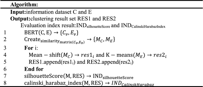
The specific algorithm design of this paper is as follows.

• Step 1. Use BERT pre-training model to build BERT server and client on the device.

• Step 2. Randomly select from the two original datasets to get two new datasets C and E.

• Step 3. Input C and E into the BERT model to generate the corresponding vector file.

• Step 4. Calculate the generated vector to get the cosine similarity, and at the same time, create the similarity matrix M.

• Step 5. Clustering by k-means and mean-shift. The input parameters are the similarity matrix and the number of communities, and the clustering results of the corresponding communities are obtained, namely RES.

• Step 6. $\mathrm{silhouetteScore}(\mathrm{M},\mathrm{RES})\to {\mathrm{IND}}_{\mathrm{silhouetteScore}}$: Obtain the value of silhouette coefficient.

• Step 7. $\mathrm{calinski}\_\mathrm{harabaz}\_\mathrm{index}(\mathrm{M},\mathrm{RES})\to {IND}_{CalinskHarabaz}$: Obtain the value of Calinski-Harabaz Index.

  

4 Experimental Analysis

4.1 Experimental Design

• I. Experimental environment

  Processor: Inte(R) Core(TM) i5-8300H CPU@2.30GHz; RAM: 8GB; Operating system: windows server 2012 R2 standard:IDE: pycharm.

• II. DataSet

  This experiment uses two datasets (toutiao_cat_data and CORD-19-research-challenge) for testing. In this experiment, for the above two datasets, 1,024 and 2,048 data were randomly selected to obtain the experimental results.

The URLs of datasets are listed as follows.

The URL of toutiao_cat_data is addressed as https://github.com/aceimnorstuvwxz/toutiao-multilevel-text-classfication-dataset.

The URL of CORD-19-research-challenge is addressed as https://www.kaggle.com/allen-institute-for-ai/CORD-19-research-challenge.

4.2 Evaluation Indices

Silhouette coefficient [11]: Silhouette coefficient is an index used to measure the effectiveness of clustering. It can describe the sharpness of each category after clustering. The profile coefficient contains two factors: cohesion and separation.

Cohesion: reflects the closeness of a sample point to the elements in the class.

Separation: reflects the closeness of a sample point to elements outside the class.

The formula of the silhouette coefficient is as follows.

$$ S(i) = \frac{b(i) - a(i)}{{max\left\{ {a(i),b(i)} \right\}}}. $$

(2)

Among them, a(i) represents the cohesion degree of the sample points, and the calculation formula is as follows.

$$ a(i) = \frac{1}{n - 1}\sum {{\text{distance}}(i,j)} . $$

(3)

Where j represents other sample points in the same class as sample i, and distance represents the distance between i and j. So the smaller a(i), the tighter the class. The calculation method of b(i) is similar to that of a(i). The value range of the silhouette coefficient S is [−1, 1]. The larger the silhouette coefficient, the better the clustering effect.

Calinski-Harabaz(CH) Index [12]: The clustering model is an unsupervised learning model. Generally speaking, the clustering result is that the closer the data distance between the same categories, the better, and the farther the data distance between different categories, the better. The CH index measures the tightness within a class by calculating the sum of the squares of the distances between each point in the class and the center of the class, and measures the separation of the dataset by calculating the sum of the squares of the distances between various center points and the center of the dataset. The CH index is obtained from the ratio of separation and compactness. Therefore, the larger the CH, the tighter the cluster itself, the more dispersed the clusters, that is, the better clustering results. The CH index is calculated as follows.

$$ {\text{s}}(k) = \frac{{tr(B_{k} )}}{{tr(W_{k} )}}\frac{m - k}{{k - 1}}. $$

(4)

Where m is the number of training set samples, k is the number of categories, Bk is the covariance matrix between categories, W_k is the covariance matrix of the data within the category, and tr is the trace of the matrix. It can be seen from the above formula that the smaller the covariance of the data within the category, the better, the larger the covariance between categories, the better, so the Calinski-Harabaz score will be higher.

4.3 Analysis of Experimental Results

Perform clustering operations on the two datasets respectively, and combine the BERT model to complete the construction of the text word vector matrix to obtain the similarity matrix. Under the premise of ensuring accuracy, reduce the time loss in the community discovery process, and finally achieve the purpose of paper classification. The analysis results are discussed as follows.

CORD-19-research-challenge Dataset

On this dataset, we selected 2,048 thesis topics, input the BERT model to generate word vectors for the topics, calculate the cosine similarity between vectors, and generate the similarity matrix that is 2,048*2,048. Then the mean-shift clustering is used for classification. Finally, use Silhouette coefficient and Calinski-Harabaz Index evaluate the performance of the process. The specific results are as follows (Fig. 2):

Fig. 2.

Three-dimensional similarity matrix of the CORD-19-research-challenge dataset.

The conclusion is obtained by using Mean-Shit clustering: Fig. 3 uses the contour coefficient to evaluate the clustering effect. It can be seen from the figure that when the number of communities decreases, the clustering effect is obviously better, and the effect of categorizing papers is also the best at this time; Fig. 4 uses the Calinski-Harabaz index to analyze the data. When the community increases, the CH indicator gradually becomes smaller. According to the nature of the evaluation index, it can be known that the steeper the curve, the better the classification effect. From the general trend of the curve in the figure, it can be estimated that then the number of classification communities is about 2, the classification effect is the best and the research significance is the greatest.

Fig. 3.

The analysis result of the evaluation index using the silhouette coefficient in the CORD-19-research-challenge dataset.

Fig. 4.

The analysis results of the evaluation indicators using the Calinski-Harabaz Index in the CORD-19-research-challenge dataset.

Toutiao_cat_data Dataset

The original dataset contains 382,688 pieces of information, which are distributed in 15 categories. We selected 1,024 pieces of data for experimentation. The operation is the same as the previous dataset, except that when clustering the data, we use K-means instead of mean-shift. Similarly, at the end of the experiment, Silhouette coefficient and Calinski-Harabaz Index are used to evaluate the classification effect of the process. The specific results and analysis are as follows (Fig. 5).

Fig. 5.

Three-dimensional similarity matrix of the toutiao_cat_data dataset.

Fig. 6.

The analysis result of the evaluation index using the silhouette coefficient in the toutiao_cat_data dataset.

The conclusion is obtained by using K-means clustering: Fig. 6 also uses the contour coefficient to evaluate the clustering effect. From the curve in the figure, it can be known that the smaller the number of communities, the better the clustering effect. At this time, the data is also The effect of centralized information classification is the best; Fig. 7 uses the Calinski-Harabaz index to evaluate the clustering results. When the number of communities increases, the CH indicator gradually becomes smaller, and the steeper the curve, the better the classification effect. It can be seen from the figure that when the number of classification communities is about 3, the classification effect is the best.

Fig. 7.

The analysis results of the evaluation indicators using the Calinski-Harabaz Index in the toutiao_cat_data dataset.

5 Conclusions

This paper uses a relatively new word vector model to process the text data and achieves a more optimistic classification effect through a series of operations. This method improves the accuracy of classic clustering algorithms, such as K-means, mean-shift, and so on. Firstly, the BERT model is used to extracts the title of the paper in the CORD-19-research-challenge dataset and the information in the dataset--toutiao_cat_data to complete the generation of the word vector, and at the same time, construct the cosine similarity matrix. Then on the premise of ensuring accuracy, the time loss in the community detection process is reduced. Finally, K-means and mean-shift are used for clustering on the two datasets, and finally, the purpose of text classification is achieved. Through the analysis of the clustering effect of the dataset, for the CORD-19-research-challenge dataset, the experimental results show that when the number of communities is 2, the clustering effect is the best. For the dataset-- toutiao_cat_data, it can be concluded that when the number of communities is 3, the clustering effect is the best. we can achieve the experimental purpose well, which provides an operational basis for information security technology to a certain extent, and need to improve the clustering operation, so as to achieve the best classification effect of the results.

References

Zhang, Q., Havard, M., Ford, E.C.: Categorizing incident learning reports by narrative text clustering to improve safety. Int. J. Radiat. Oncol. Biol. Phys. 108(3), S55 (2020)
Amer, A.A., Abdalla, H.I.: A set theory based similarity measure for text clustering and classification. J. Big Data 7(1), 1–43 (2020). https://doi.org/10.1186/s40537-020-00344-3
Shen, S., Liu, X., Sun, H., Wang, D.: Biomedical knowledge discovery based on Sentence‐BERT. Proc. Assoc. Inf. Sci. Technol. 57(1) (2020)
Ambalavanan, A.K., Devarakonda, M.V.: Using the contextual language model BERT for multi-criteria classification of scientific articles. J. Biomed. Inform. 112, 103578 (2020)
Zheng, J., Wang, J., Ren, Y., Yang, Z.: Chinese sentiment analysis of online education and Internet buzzwords based on BERT. J. Phys. Conf. Ser. 1631(1) (2020)
Park, K., Hong, J.S., Kim, W.: A methodology combining cosine similarity with classifier for text classification. Appl. Artif. Intell. 34(5), 396–411 (2020)
Liu, D., Chen, X., Peng, D.: Some cosine similarity measures and distance measures between q -rung orthopair fuzzy sets. Int. J. Intell. Syst. 34(7), 1572–1587 (2019)
Ahmed, M., Seraj, R., Islam, S.M.S.: The k-means algorithm: a comprehensive survey and performance evaluation. Electronics 9(8) (2020)
Li, J., Chen, H., Li, G., He, B., Zhang, Y., Tao, X.: Salient object detection based on meanshift filtering and fusion of colour information. IET Image Proc. 9(11), 977–985 (2015)
Du, Y., Sun, B., Lu, R., Zhang, C., Wu, H.: A method for detecting high-frequency oscillations using semi-supervised k-means and mean shift clustering. Neurocomputing 350, 102–107 (2019)
Nidheesh, N., Abdul Nazeer, K.A., Ameer, P.M.: A hierarchical clustering algorithm based on silhouette index for cancer subtype discovery from genomic data. Neural Comput. Appl. 32(15), 11459–11476 (2019). https://doi.org/10.1007/s00521-019-04636-5
Putri, D., Leu, J.-S., Seda, P.: Design of an unsupervised machine learning-based movie recommender system. Symmetry 12(2), 185 (2020). https://doi.org/10.3390/sym12020185
Acknowledgments
This research was partially supported by National Key Research and Development Program of China (No. 2018YFB1201500) and Natural Science Foundation of China (No. 61773313).
Author information
Authors and Affiliations
Corresponding author
Editor information
Editors and Affiliations
Rights and permissions
Copyright information
© 2021 Springer Nature Switzerland AG
About this paper
Cite this paper
Zhang, K., Hei, X., Fei, R., Guo, Y., Jiao, R. (2021). Cross-Domain Text Classification Based on BERT Model. In: Jensen, C.S., et al. Database Systems for Advanced Applications. DASFAA 2021 International Workshops. DASFAA 2021. Lecture Notes in Computer Science(), vol 12680. Springer, Cham. https://doi.org/10.1007/978-3-030-73216-5_14
Download citation
DOI: https://doi.org/10.1007/978-3-030-73216-5_14
Published:
Publisher Name: Springer, Cham
Print ISBN: 978-3-030-73215-8
Online ISBN: 978-3-030-73216-5
eBook Packages: Computer ScienceComputer Science (R0)