
Abstract
Flexible AC Transmission Systems (FACTS) is created higher controllability in power systems. Several FACTS-devices are introduced for various applications. The basic applications of FACTS-devices are including power flow control, voltage control, reactive power compensation, stability improvement, power quality improvement, flicker mitigation, interconnection of renewable and distributed generation and storages. But to achieve the maximum profit from FACTS devices, the optimal size and location of these devices must be determined. Numerical optimization method is one of the methods to achieve the optimal global solution in optimization problems. This chapter of the book is about FACTS devices placement using numerical method. This method is performed in a radial Transmission system to minimize the power losses and improve the voltage profile. The proposed method is tested on the standard IEEE 14-bus test system. The results of case studies demonstrate the effectiveness of the proposed methodology.
Access provided by Autonomous University of Puebla. Download chapter PDF
Keywords
1 Introduction
In the past decades, the increase in demand for electricity has led to an integrated power system with thermal and insulating limitations and issues such as the passage of power over unwanted routes and stability constraints. Experts and designers of power systems have proposed solutions to address these issues, such as the construction of a new line, Flexible Alternating Current Transmission Systems (FACTS) in transmission and distribution, and High Voltage Direct Current (HVDC). One of the disadvantages of building a new transmission line is environmental issues, and the disadvantages of HVDC are the high cost of this system. Therefore, to increase the capacity of the transmission line and improve the stability of the system, the appropriate solution is to use FACTS devices. The best solution is to use FACTS controllers to increase the capacity of distribution and transmission networks. FACTS controllers control important parameters of a transmission line (angle, voltage, current, active power, and reactive power). Applications of FACTS include improved transient stability, small signal stability improvement, voltage profile improvement, power losses reduction, and reduction of inrush currents caused by transformers. The important advantages of FACTS are shown in the Fig. 1 [1, 2].

The issue of FACTS devices is not new, as it has been built over the past 20 years using large-scale power technology and semiconductors. Today, the most important issue in FACTS controllers is the economic issue [1]. In addition to the applications mentioned above, these devices are also used to manage congestion, and reduce power losses. FACTS controllers are based on power electronics and are used in low voltage and transmission networks as series, parallel and series–parallel compensators to increase system controllability. For example, Static Synchronous Series Compensator (SSSC) and Thyristor Controlled Series Capacitor (TCSC) controllers are used as series compensators and Static Compensator (STATCOM) and Static Var Compensator (SVC) controllers are used as parallel compensators in the system. FACTS devices category will be presented later in the chapter [3].
At the beginning of the chapter, we will study the numerical techniques and solutions of MATLAB software, and in this section, we will explain the interval solution and open methods. We will then discuss the FACTS devices, the classification of FACTS controllers, the modeling, and the formulation of the optimal placement of FACTS devices. In the last part of this chapter, we will present a test system to analyze and simulate the optimal placement of SVC and UPFC controllers using Newton Raphson's numerical technique using MATLAB software.
2 Numerical Technique
Numerical analysis is widely used in the analysis of nonlinear systems in the fields of electrical and mechanical engineering, so that the MATLAB software has designed its solvers based on numerical analysis. Choosing the appropriate numerical technique to design and analyze power systems has become an important research challenge. Therefore, it is important to know numerical methods to solve nonlinear problems. In this chapter, we examine the advantages and disadvantages of widely used numerical techniques in power systems and their application in power systems. Applications of these techniques include load flow studies, maximum power point tracking (MPPT), optimal DG placement, and optimal FACTS devices placement. The first step in better understanding of these methods is to classify them. Therefore, we categorize numerical techniques into four subdivisions, taking into account their application in power systems:
-
1.
Interval solution methods
-
2.
Open methods
-
3.
Introspection
-
4.
Numerical Integration.
In addition to the above classification, MATLAB software has also solvers based on numerical techniques to solve difficult and non-difficult problems so that the user can choose the appropriate solver according to the type of system. Table 1 shows the types of MATLAB solvers. Figure 2 shows the most widely used numerical techniques in the electrical industry. It is worth noting that in the studies of researchers, interval solution methods and open methods have received more attention. Therefore, the theoretical explanations of the methods of solving the interval and open methods will be discussed.

Numerical techniques used in electrical engineering
2.1 Bisection Method [5,6,7,8,9]
In this method, we assume that the numbers a and b are available in the following ways:
-
(a)
The function f in interval [a, b] is continuous
-
(b)
f(a) · f(b) < 0
-
(c)
f(x) = 0 has only one root (α) in the range (a, b).
In this method, we make the sequence {xn} as follows:
To build this sequence, we do the following:
We first X1 consider (a + b)/2, which divides [a, b] into two parts [a, X1] and [X1, b]. Now, assuming case C, α is necessarily in one of these two parts. To continue, we consider the part where α is located, where it is possible to select the desired range through the Bolzano theorem. After selecting the desired range, we take the X2 method in the same way and continue the same process until we reach the condition of stopping the problem. Note that in the bisection method, the sequence is constructed to converge to the root of the function, and it is easy to show that:
Disadvantages include the following:
-
1.
This numerical technique is not suitable for finding double roots.
-
2.
Slow dynamically answer.
-
3.
Very slow performance when finding multiple roots.
Application of this numerical method in smart networks include operation studies in low voltage networks.
In the reference [10], a distributed bisection technique with the presence of the small-scale resources has proposed for the economic dispatch of load on the smart networks.
Another application of this technique in power systems is the discussion of the MPPT in renewable sources such as wind turbines and photovoltaic systems.
In other words, this method can be used to increase the extraction capacity of the mentioned resources [11]. In addition to electrical engineering, this technique has many applications in other branches of engineering such as mechanics. The bisection algorithm is shown in Fig. 3.

Bisection algorithm [8]
2.2 Regula Falsi Method [5,6,7,8,9]
Assume that the function f in [a, b] is continuous and that f(a)f(b) < 0 and the equation f(x) = 0 have only one root in (a, b). Now, to find an approximation of this root, which we call α, we action as follows. Connect the two points (a, f(a)) and (b, f(b)) with a straight line, we call the intersection of this line with the axis of the x¬ x1 which approximate of the desired root is α, now to find the value of x1, we place point (x1, 0) in the equation of the line connecting the two points (a, f(a)) and (b, f(b)), that is, in Eq. 3:
We place the point (x1, 0), so we have:
After simplifying, we get to the following equation:
Now to determine x2, do the following:
-
1-
If f(a)f(x1) < 0, then according to Bolzano's theorem the root α is in (a, x1), so in formula 5 instead of b, we put x1 and we have:
$$x_{2} = \frac{{af(x_{1} ) - x_{1} f(a)}}{{f(x_{1} ) - f(a)}}$$(6) -
2-
If f(a)f(x1) > 0, then the root is in (x1, b). So in formula 5, instead of a, we put x1 and we have:
$$x_{2} = \frac{{x_{1} f(b) - bf(x_{1} )}}{{f(b) - f(x_{1} )}}$$(7) -
3-
If f(a)f(x1) = 0 then it is clear that x1 is the desired root and the problem is solved.
Thus, a sequence of numbers is obtained that converges to the root α. As you can see, the Regula Falsi method is convergent similar to the Bisection method. Sometimes it works even faster than the Bisection method. Of course, the operation of this method is more than the two-part method. See Fig. 4 for more details.

Details of Regula Falsi method [8]
2.3 Simple Repetition or Fixed Point Method [5,6,7,8,9]
In this method, by applying changes in the equation f(x) = 0 to x = g(x), if α is the root of f(x), then g(α) = α. In fact, the root of f will be a fixed point g.
Fixed point theorem:
Suppose that \(g:[a,b] \to [a,b]\) function is a continuous function (\(g \in c\left[ {a,b} \right]\)) in this case:
-
(A)
g has at least one fixed point in [a, b]. In addition, if g’ is present on the interval (a, b) and the number \(0 < L < 1\) is present so that we have \(\left| {g^{\prime } (x)} \right| \le L < 1\) for each x in (a, b), then the constant point g in [a, b] is unique.
-
(B)
The sequence produced by \(x_{n + 1} = g(x_{n} )\) that \(n = 0,1,2,3,...\) is convergent for each \(x_{0} \in [a,b]\) to the constant point g (root f). To better understand the fixed point technique, consider Fig. 5.
Fig. 5 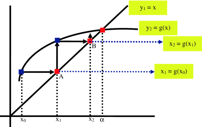
Details of fixed point method [8]

2.4 Newton Raphson Method [5,6,7,8,9]
This numerical technique works faster than other methods mentioned above. However, in this method, the starting point of x0 must be close enough to the desired root α, which is one of the disadvantages of this method. After explaining how this method works, you will clearly see that there is a special case of the simple repetition method mentioned. Now, with the help of Fig. 6, we will describe this method.

Newton Raphson method [8]
If x0 is approximate to the desired root, α. As you can see in the figure, we draw the tangent line of the curve f(x) at point A to the coordinates (x0, f(x0)). We call the location of this line the axis of length x1. In fact, by placing a point (x1, 0) in Eq. 8 and continuing this process, we achieve a repetitive design of Newton method (9).
So we will have:
Given the Eq. 10, it is clear that Newton's method is a special case of the simple repetition method.
Newton Raphson method is shown in Fig. 7.

Newton Raphson algorithm [8]
2.5 Secant Method [5,6,7,8,9]
First, consider the Eq. 11, which is the derivative definition.
If the value of x is close to the value of xn, for example, xn-1, then:
In the Newton formula, we use Eq. 12 instead of f ‘(xn), and after simplification, we will have:
Note that we need the values initial two of x0 and x1 in the Secant method for calculating xn. Then the rest of the sequence of sentences is easily obtained through Eq. 13. The Secant method is not necessarily convergent and is slower than Newton in terms of speed, but much faster than the Bisection method and the Regula Falsi technique. Note Fig. 8 for further explanation.

Secant method [8]
One of the most important issues in smart grids is the discussion of MPPT from renewable sources such as photovoltaic systems and wind turbine systems. Because the mentioned sources are facing uncertainties such as the amount of sunlight and wind speed. In recent years, many studies and researches have been done in the field of MPPT in low voltage networks.
The researcher in the reference [11] used numerical techniques to investigate the tracking of the MPPT in photovoltaic systems. Figure 9 shows the MPPT controller for a photovoltaic system and Fig. 10 shows the performance of numerical techniques.

MPPT controller for a photovoltaic system

Performance of numerical techniques [11]
Numerical optimization methods can ensure the global optimal solution. Also, used methods in [12,13,14,15] are to achieve global optimal.
3 FACTS Devices
The flow of active and reactive power (the flow of current leads to the flow of power.) In a transmission line between the two buses i and k shown in Fig. 11 of the Eqs. 14 and 15 are calculated [16]:

Active and reactive power flow
- Vi and Vk:
-
The magnitudes of the bus voltages i and k.
- Xik:
-
Reactor Transmission Line.
- δik:
-
power transfer angle.
FACTS controllers are divided into three classes based on the type of compensation, series (injecting voltage into the system in series), parallel (their connection is parallel and at the connection point, the current is injected into the system) and series–parallel are classified. The effect of some FACTS controllers on Eq. 14 is shown in Fig. 12 [16].

Effect of FACTS controllers [16]
The classification of FACTS device controllers, the structure of the famous FACTS machines, and the use of the famous FACTS devices are shown in Figs. 13, 14 and 15, respectively. So, SSSC, Interline Power Flow Controller (IPFC), TCSC, Thyristor Switched Series Capacitor (TSSC), Thyristor Controlled Series Reactor (TCSR), Thyristor Switched Series Reactor (TSSR), SVC, Thyristor Controlled Reactor (TCR), Thyristor Switched Reactor (TSR), Thyristor Switched Capacitor (TSC), STATCOM, Static Synchronous Generator (SSG), Battery Energy Storage System (BESS), Superconducting Magnetic Energy Storage(SMES), UPFC, TCPST, Thyristor Controlled Phase Angle Regulator (TCPAR), Interphase Power Controller (IPC), Thyristor Controlled Voltage Limiter (TCVL) and TCVR are specified in the figures.

FACTS controllers’ classification [2]


The structure of the famous FACTS devices [17]

Application of well-known FACTS devices [17]
3.1 Power System Modeling
The first step in the study of power systems, such as the optimal placement of FACTS controllers, is to provide the correct model of the system under study. In other words, if the model is not presented correctly, the objectives of the studies will not be achieved.
The mathematical model of the power system shown in Fig. 16 is defined in Eqs. 16–23 [18, 19].

Power system model [18]
The mathematical model of the load is shown in Eq. 24 [18]:
C represents the constant capacitor, V represents the load voltage, δ represents the phase voltage of the load voltage, ωm the rotor speed, δm the phase angle of the generator, M the inertia of the generator, dm dumping and Pm express the mechanical power [18, 19].
3.2 SVC Modeling
In this device, changing of load and topology of the system will affect the bus voltage. Therefore, in case of improper control, the voltage will drop and may even lead to network collapse. Conventional devices such as capacitors, reactors (conventional devices controlled by mechanical switching), and rotating synchronous condenser can be used to adjust the voltage of the buses that are out of range. The injection or absorption of reactive power is automatically adjusted by the SVC and the rotating synchronous condenser to keep the voltage across the buses constant. SVC is a combination of capacitive and induction banks with thyristor control or mechanical switching control as shown in Fig. 7. To conduct numerical studies, SVC is classified into two models [20]:
-
1.
shunt variable susceptance model
susceptance is considered as a mode variable in a state-space equations and formulations. The shunt variable susceptance model is shown in Fig. 17 [21, 22].

-
2.
Fire angle model
Fire angle is considered as a mode variable in Eqs. and formulations. The fire angle model is shown in Fig. 18 [21, 22].

Figure 19 shows the dynamic characteristics and the steady-state voltage and current of the SVC controller. In the SVC controller, we only exchange reactive power. Therefore, the susceptance, current, and reactive power are changed to adjust the voltage according to a desirable characteristic with a suitable slope (slope value is usually considered between 1 and 5%) [21].

Dynamic characteristics, steady state mode voltage, and SVC current controller [21]
The amount of slope depends on the desired voltage (the optimum voltage is defined in the controllable area), the production of reactive power between different sources (considering optimal conditions for the system), and attention to other needs of the system. Figure 19 shows that the SVC compensates for the reactive power in the system in a capacitive region such as a shunt capacitor and in an inductive section such as a shunt reactor. In the following, we provide a numerical analysis of the fire angle model and the variable susceptance model of the SVC controller (considering sine voltage). The ISVC is defined according to Eq. 25 [21].
XTCR is defined according to Eq. 26 [21, 22].
We know that \(X_{L} = \omega L\), now we have a Eq. by placing \(\sigma = 2(\pi - \alpha )\) [21, 22].
In the Equations mentioned, σ indicates conductivity, and α indicates fire angles. If α = 90, the TCR will be fully conductive. In other words, XTCR will be equal to XL. If α = 180, the TCR conductivity will be zero, and the reactance will be infinite. SVC reactance is a combination of a capacitor and TCR reactance listed in Eq. 28 [21, 22].
We know that \(X_{C} = \frac{1}{\omega C}\), then we define QK according to Eq. 29 [21, 22].
On the other hand, the SVC equivalent susceptance is defined according to Eq. 30 [21, 22]:
3.2.1 Power Flow Model
The equations for the linearized power flow of the SVC controller are shown in Table 2 based on the shunts variable susceptance models and fire angle [20, 23].
3.2.2 SVC Controller Model
The SVC diagram block with a classic PI controller is shown in Fig. 20. XSVC is modified using fire angle control (this change is done with the help of a classical controller) to adjust the voltage within the allowable range [21, 22].

According to the figure above, the state equations \(\dot{X}_{1SVC}\), \(\dot{X}_{2SVC}\), and \(\dot{X}_{3SVC}\) according to Eq. 31 are defined [21, 22].
QSVC reactive power is expressed according to Eq. 32 [21]:
In the following, we will perform the Eqs. 31 and 32 [21, 22]:
Finally, we will have the Eq. 34 [21, 22]:
Equation 34 can be summarized in the form of Eq. 35 [21, 22]:
3.2.3 SVC Connection in Multi-machine Power Systems
Equilibrium power equations for the optimal placement of the SVC controller in multi-machine power systems are defined according to Eq. 36 [21, 22].
After the linearization of the above equations, the Eq. 37 is obtained [21, 22].
Considering the SVC controller, the DAE model is defined according to Eq. 38 [21, 22]:
3.3 TCSC Modeling
As mentioned in the FACTS devices, the TCSC controller is a series of compensators and increases the transmission capacity by changing the appearance impedance of the transmission line. The structure of the TCSC series controller is shown in Fig. 21. The XTCSC steady-state impedance is defined by Eq. 39 [21].

TCSC series controller structure [21]
XL (α) is defined according to Eq. 40 [21]:
3.3.1 TCSC Controller Model
The TCSC controller is very similar in structure to the FC-TCR SVC controller. Equivalent impedance is presented for this series compensator in Eq. 41 [21, 22].
- α::
-
Fire angle.
- σ::
-
conductivity angle.
- k::
-
TCSC ratio.
The TCSC controller usually operates in the capacitor area. A very important point in the series controllers is the resonance. Figures 22 and 23 show the equivalent reactance and susceptance of SVC and TCSC controllers, respectively. The resonance in the SVC controller does not appear to be a problem, but in the TCSC series controller, a range must be defined for the fire angle. Therefore, the fire angle range for the TCSC controller is defined by considering the resonance point according to Eq. 42 [22]:

Equivalent reactance to the SVC controller [22]

Equivalent reactance to the TCSC controller [22]
3.3.2 TCSC Controller Model
As Fig. 24, the TCSC controller is located between bus k and m. If the TCSC controller losses are neglected, the power equilibrium and BTCSC equations are defined according to Eq. 43 [21].

TCSC connection in multi-machine power systems [21]
Table 3 are shown 4 control strategies for TCSC in [21, 22].
Each of the strategies listed in the table above can be used to achieve TCSC controller goals. Here are some numerical studies of the power control strategy. Figure 25 shows the block diagram of the TCSC controller with the PI controller [21, 22].

\(X_{2TCSC}\), \(\dot{X}_{2TCSC}\) and \(\dot{X}_{1TCSC}\) are defined according to Eq. 44 [21, 22].
After linearization we will have [21, 22]:
The DAE model of the TCSC controller is defined by Eq. 46 [21, 22].
As a result, we will have [21, 22].
3.4 UPFC Modeling
As shown in Fig. 26, the UPFC Series–Parallel Controller consists of two series and parallel converters connected by a DC link [24].

UPFC structure [24]
In the following, we will study UPFC numerical studies using Newton Raphson method. According to Fig. 27, the UPFC equivalent circuit consists of two ideal voltage sources. Zser and Zsh represent the series and parallel impedance, respectively, and consist of a positive sequence of leakage resistance and inductance. The relationship between ideal voltage sources is expressed in Eq. 48 [24, 25].

UPFC injection model [24]
According to the injection model (equivalent circuit) UFPC, Eqs. 49 and 50 introduce the limitations of Vser and ϴser, respectively [24, 25]:
According to the UFPC equivalent circuit, Eqs. 51 and 52 show the constraints of Vsh and ϴsh, respectively [24, 25].
According to the above equations, the equations for active and reactive power of UPFC in node i are given in Eqs. 53 and 54, respectively [24, 25]:
The Eqs. of active and reactive power of UPFC in node j are also defined according to Eqs. 55 and 56 [24, 25].
The shunt converter reactive and active power relations are described in the following equation [24, 25].
The active power relation of the series converter is introduced in the following equation [24, 25]:
The reactive power relative of the series converter is introduced in the following equation [24, 25]:
Yii, Yjj, Yij, and Yser admittances are defined according to the following equations: [24]:
Assuming low switching losses of series and parallel converters, the following equation will be established [24, 25]:
In the next step of the study, we must combine the linearized power equations of the FACTS controller with the linear equations of the system (the rest of the network). Therefore, the following equation is defined [24]:
In the mentioned relationship, [ΔX] the solution vector, [J] the Jacobin matrix and ΔPbb matrixes of the incompatibility of the power obtained from the Eq. 62. The solution vector is defined according to Eq. 65 [24].
Jacobin matrix is given according to [24, 25] in Eq. 66:
The initial conditions of the series and parallel sources are shown in Eqs. 67 and 68, respectively [24].
4 Formulation the Problem of FACTS Devices Placement
To solve the problem of economic placement of FACTS controllers in power systems, the objective functions and constraints of the problem must first be determined. Therefore, we will describe the mentioned cases [26].
4.1 Objective Functions
Important objective functions in FACTS controller placement studies include voltage deviation, system overload, and active power losses. In other words, we are dealing with a multi-objective optimization problem when discussing the placement of FACTS devices. Formulation of a multi-objective optimization problem in Eq. 69 is given in which x is the decision variable, Ω is the solution range, Cj (x) is the equal constraint, Hk (x) is the unequal constraint, Fv (x) is the objective function of the voltage deviation, Fs (x) is the objective function of the system overload and FPL (x) is the objective function of active power losses [26].
4.2 Constraints
Constraints on the optimal placement of FACTS controllers to two categories of equality constraints (e.g. active power equilibrium) and unequal constraints (e.g. allowable voltage range, reactive power output limit, FACTS devices limitations such as compensation range) Are divided [26].
4.2.1 Equality Constraints
In Eq. 70, the equilibrium of active and reactive power is mentioned [26]:
4.2.2 Inequality Constraints
In Eq. 71, the limitation of reactive power generation and in Eq. 72 the limitation of some FACTS controllers such as SVC, TCSC and UPFC are given [26].
The objective functions used to optimally placement of FACTS devices in researchers’ studies are shown in Fig. 28 [17].

Objective functions for optimal placement of FACTS devices [17]
4.3 Optimal Placement of TCSC, SVC, and UPFC
The correct choice of bus and line in the system under study to optimal placement of the FACTS devices controllers such as SVC, TCSC, and UPFC depends on the network structure. For example, SVCs (TCR, TSR, and TSC) are used to correct the total reactive power flow between buses. TCSCs are commonly used to change line impedance to control the power flow in transmission lines. UPFC, as shown in Fig. 15, is a complete controller and is used to improve voltage and increase line capacity [27].
TCSCs are used as FACTS devices series controllers using the Lmn index specified in weak lines. Lmn is one of the appropriate indicators that can be analyzed in lines that are unstable. This indicator says that if Lmn is equal to one, the state of the critical line is. If Lmn is less than one, it indicates the stable state of the line. The Lmn index is given in Eq. 73 [27, 28].
x represents the line, Qr indicates the demand for reactive power, Vs indicates the bus voltage of the sending side, ϴ indicates the difference between the bus angles, and δ indicates the impedance angle. The optimal placement of the SVC controller, which is connected in parallel, is done by analyzing the PV curves. It should be noted that PV curves are made using the CPF technique. The predictive and correction scheme used in CPF is shown in Fig. 29. Optimal placement by UPFC is done on lines where the high active power flow has, it should also be noted that UPFCs are placed at the beginning of the buses to play their role as a complete FACTS devices series–parallel controller [27, 29].

Predictive and correction scheme used in CPF [29]
The objective functions and the optimal location and size limitations of FACTS devices [27] are shown in Table 4:
Example 1:
In the 14-bus distribution system is shown in Fig. 30, the 5 SVCs placement perform with a capacity of 5 MW. Then, the SVCs place in the selected locations. Compare the voltage profile with SVC mode. Perform the placement with the Newton Raphson method to improve the voltage profile. Select buses to be placed in buses without any power plant. Then place the SVC in the selected locations and use Newton Raphson method to check the system's performance in terms of voltage and power losses before and after the SVC.

IEEE 14-bus test system
Solution: In this example, the SVC was replaced to improve the voltage profile. The proposed method is that to placement the first bus voltages are obtained by Newton–Raphson method. Then, according to the obtained voltages, 5 buses with the lowest voltage are selected for SVC installation. The buses selected for placement are: 4-5-10-13-14. Then, to check the performance of SVC in the system, we put the information about SVC in the base system. By placing SVC in these buses and comparing the voltage before and after SVC as shown in Fig. 31, we see that the voltage has improved significantly that indicate suitable performance of in improving system voltage levels. The active and reactive power losses without SVC mode are 13,393 MW and 54.54 MVAR respectively. While the power losses after SVC installation are 13,345 MW and 54.22 MVAR. By adding SVC, 48 MW is reduced for the active power and 320 kVAR for reactive power, indicating suitable performance of SVC in reducing system power losses. To better check the voltage profile, we can check the voltage stability indices in offline in both cases using the following relationships:

Voltage profile before and after SVC placement
That VSF is: Voltage stability Factor. Considering the above two equations, we check the voltage stability in each case with and without SVC. without SVC mode, VSF is 1.0514 p.u. While in SVC mode, the VSF increases by 1.0625 p.u.
Example 2:
In Fig. 30, install one UPFC with the goal of improving the voltage profile. Then draw the voltage profile before and after the placement. Also determine the active and reactive power losses before and after the placement UPFC using the Newton Raphson method.
Solution: The optimal place for UPFC is selected in the line between buses 2 and 5. The voltage profile before and after placing the UPFC is shown in Fig. 32. The voltage is improved significantly after installing UPFC. The active and reactive power losses without UPFC mode are 13,393 MW and 54.54 MVAR respectively, While the power losses after installation of UPFC are 13,368 MW and 54.38 MVAR.

Voltage profile before and after UPFC placement
5 Conclusions
In this chapter, first the benefits of FACTS devices have been studied and proposed as a suitable solution for improvement of power system characteristics. Then mathematical modeling of some widely used FACTS devices such as SVC, TCSC and UPFC are described. In the following, numerical optimization methods for FACTS devices analysis are presented. Numerical optimization methods in many cases can ensure global optimization. Among the introduced methods, one of the most widely used methods in studies of power system is the Newton Raphson method. The important functions and constraints in the discussion of placement and modeling of FACTS devices are presented in this chapter for controlling power flow, regulating the bus voltage and reducing of power losses. The Newton Raphson method is considered for the equation solving of the objective functions. Finally, to demonstrate the advantage of FACTS devices, simulations for SVC and UPFC are performed on the IEEE 14 bus system. According to the results, optimal placement of FACTS devices improves most of the power system specifications.
Change history
18 May 2021
The original version of these chapters “Numerical Methods in Selecting Location of Distributed Generation in Energy Network” and “Numerical Methods for Power System Analysis with FACTS Devices Applications” are inadvertently published with branch name after the institution name. It has now been corrected.
Abbreviations
- Vi:
-
The magnitude of voltage at bus i.
- Vj:
-
The magnitude of voltage at bus j.
- Vm:
-
The magnitude of voltage at bus m.
- Vk:
-
The magnitude of voltage at bus k.
- V:
-
The load voltage.
- Vser:
-
Controllable voltage source in series branch.
- Vsh:
-
Controllable voltage source in parallel branch.
- Pm:
-
Mechanical power.
- Pik:
-
Active power flow between the two buses i and k.
- Pk:
-
Active power flow between the two buses k and m.
- Pm:
-
Active power flow between the two buses m and k.
- Pi:
-
Active power of UPFC in node i.
- Pj:
-
Active power of UPFC in node j.
- Psh:
-
The shunt converter active power.
- Pser:
-
The series converter active power.
- PGi:
-
Active power generation.
- PDi:
-
Active power consumption.
- Qik:
-
Reactive power flow between the two buses i and k.
- Qk:
-
Reactive power flow between the two buses k and m.
- Qm:
-
Reactive power flow between the two buses m and k.
- Qi:
-
Reactive power of UPFC in node i.
- Qj:
-
Reactive power of UPFC in node j.
- Qsh:
-
The shunt converter reactive power.
- Qser:
-
The series converter reactive power.
- QGi:
-
Reactive power generation.
- QDi:
-
Reactive power consumption.
- Xik:
-
Reactor transmission line.
- δik:
-
Power transfer angle.
- C:
-
The constant capacitor.
- ωm:
-
The rotor speed.
- δ:
-
The phase voltage of the load voltage.
- M:
-
The inertia of the generator
- x:
-
The decision variable.
- [ΔX]:
-
The solution vector.
- [J]:
-
The Jacobin matrix.
- Ω:
-
The solution range.
- Cj (x):
-
The equal constraint.
- Hk (x):
-
The unequal constraint.
- Fv (x):
-
The objective function of the voltage deviation.
- Fs (x):
-
The objective function of the system overload.
- FPL (x):
-
The objective function of active power losses.
- Lmn:
-
Line stability index.
- VSF:
-
Voltage stability factor.
- α:
-
Fire angle.
- σ:
-
Conductivity angle.
- k:
-
TCSC ratio.
- B:
-
Susceptance.
- Y:
-
Admittance.
References
Bayliss C, Hardy B (2012) Transmission and distribution electrical engineering. Elsevier
Hingoranl NG (2000) Understanding facts. Wiley
Singh AK, Pal B (2018) Dynamic estimation and control of power systems. Academic Press
Xu K (2014) Time dependent performance analysis of wireless networks. Dissertation, University of Pittsburgh
Burden RL, Faires JD, Burden AM (2010) Numerical analysis: Cengage Learning
Cheney EW, Kincaid DR (2012) Numerical mathematics and computing. Cengage Learning
Hamming R (2012) Numerical methods for scientists and engineers. Courier Corporation
Babolian E (2020) Numerical analysis 1. Payame Noor University. Pnueb. https://www.pnueb.com/courses/ls/228/86. Accessed 23 May 2020
Ralston A, Rabinowitz P (2001) A first course in numerical analysis. Courier Corporation
Xing H et al (2014) Distributed bisection method for economic power dispatch in smart grid. IEEE Trans Power Syst 30(6):3024–3035
Seunghyun C (2015) Integration of mathematics for sustainable energy applications. In: 2015 ASEE annual conference & exposition, Seattle, Washington, June 2015, ASEE Conferences
Choopani K, Hedayati M, Effatnejad R (2020) Self-healing optimization in active distribution network to improve reliability, and reduction losses, switching cost and load shedding. Int Trans Electr Energy Syst 30(5):e12348
Choopani K, Effatnejad R, Hedayati M (2020) Coordination of energy storage and wind power plant considering energy and reserve market for a resilience smart grid. J Energy Storage 30:101542
Vazinram F et al (2020) Self-healing model for gas-electricity distribution network with consideration of various types of generation units and demand response capability. Energy Convers Manag 206:112487
Vazinram F et al (2019) Decentralised self-healing model for gas and electricity distribution network. IET Gener Transm Distrib 13(19):4451–4463
Ghahremani E, Kamwa I (2012) Optimal placement of multiple-type FACTS devices to maximize power system loadability using a generic graphical user interface. IEEE Trans Power Syst 28(2):764–778
Ahmad AL, Sirjani R (2019) Optimal placement and sizing of multi-type FACTS devices in power systems using metaheuristic optimisation techniques: an updated review. Ain Shams Eng J
Dobson I et al (1988) A model of voltage collapse in electric power systems. In: Proceedings of the 27th IEEE conference on decision and control, vol 3. IEEE
Liaw D-C, Chen J-W, Huang Y-H (2018) A Numerical study of the SVC-controlled electric power system dynamics. Int J New Technol Res 4(6):10–15
Ambriz-Perez H, Acha E, Fuerte-Esquivel CR (2000) Advanced SVC models for Newton-Raphson load flow and Newton optimal power flow studies. IEEE Trans Power Syst 15(1):129–136
Singh B et al (2018) Utilities of differential algebraic equations (DAE) model of SVC and TCSC for operation, control, planning & protection of power system environments. Int J Futur Revolut Comput Sci Commun Eng 4(1):61–67
Welhazi Y et al (2014) Power system stability enhancement using FACTS controllers in multimachine power systems. J Electr Syst 10(3):276–291
Pali BS, Bhowmick S, Kumar N (2012) Newton-Raphson power flow models of static VAR compensator. In: 2012 IEEE 5th India international conference on power electronics (IICPE). IEEE
El-Sadek MZ et al (2007) Comprehensive Newton-Raphson model for incorporating unified power flow controller in load flow studies. J Eng Sci 35(1):189–205
Acha E et al (2004) FACTS: modelling and simulation in power networks. Wiley
El-Arini MM, Ahmed RS (2012) Optimal location of FACTS devices to improve power systems performance. J Electr Eng 12(3):73–80
Nadeem M et al (2020) Optimal placement, sizing and coordination of FACTS devices in transmission network using whale optimization algorithm. Energies 13(3):753
Moghavvemi M, Omar FM (1998) Technique for contingency monitoring and voltage collapse prediction. IEE Proc Gener Transm Distrib 145(6):634–640
Ajjarapu V, Christy C (1992) The continuation power flow: a tool for steady state voltage stability analysis. IEEE Trans Power Syst 7(1):416–423
Author information
Authors and Affiliations
Corresponding author
Editor information
Editors and Affiliations
Rights and permissions
Copyright information
© 2021 The Author(s), under exclusive license to Springer Nature Switzerland AG
About this chapter

Cite this chapter
Hedayati, M., Effatnejad, R., Choopani, K., Chanddel, M. (2021). Numerical Methods for Power System Analysis with FACTS Devices Applications. In: Mahdavi Tabatabaei, N., Bizon, N. (eds) Numerical Methods for Energy Applications. Power Systems. Springer, Cham. https://doi.org/10.1007/978-3-030-62191-9_35
Download citation
DOI: https://doi.org/10.1007/978-3-030-62191-9_35
Published:
Publisher Name: Springer, Cham
Print ISBN: 978-3-030-62190-2
Online ISBN: 978-3-030-62191-9
eBook Packages: EnergyEnergy (R0)