Arithmetic Aspects of Orbifold Pairs

Abstract

Let X be a smooth connected projective manifold defined over a number field k. We give below a conjectural qualitative description of X(k’) for k’ a sufficiently large number field containing k according to the algebro-geometric positivity/negativity of the cotangent bundle of X. When X is ‘of general type’, our conjecture coincides with Lang’s conjecture claiming the ‘Mordellicity’ of X . In the general case, we decompose X by means of a new fibration, its ‘core map’, the fibres of which are ‘special’, its ‘orbifold base’ being of ‘general type’. The ‘special’ manifolds generalise rational and elliptic curves, and we conjecture them to be ‘potentially dense’. Extending Lang’s (and Vojta’s) conjecture to the orbifold setting, we get the above conjectural qualitative description of X(k’). Even for orbifold curves, our conjecture is open, but is implied by the abc-conjecture.

1 Introduction

Let X be a smooth connected projective manifold of dimension n defined over a number field k, let k′⊃ k be a larger number field. We denote by X(k′) the set of k′-rational points of X. Diophantine geometry aims at describing, in terms of the ‘geometry’ of X(ℂ), the qualitative structure of X(k′) when k′ is sufficiently large, depending on X. When k is too small, the paucity of X(k) may indeed be related not only to the geometry of X(ℂ), but also to the coefficients of the equations¹ defining X, as seen on the rational curve x ² + y ² + 1 = 0 for k = ℚ, and $k'=\Bbb Q(\sqrt {-1})$.

Definition 1.1

We say that X∕k is ‘potentially dense’ if X(k′) is Zariski dense ² in X for some k′⊃ k, k′ depending on X.

The opposite property is X being ‘Mordellic’, ³ which means the existence of a nonempty Zariski open subset U ⊂ X such that (X(k′) ∩ U) is finite for any k′⊃ k.

A curve is thus either Mordellic or potentially dense, according to whether X(k′) is finite for any k′∕k, or infinite for some k′∕k. A curve X∕k of genus g is potentially dense if and only if g = 0, 1, curves of genus g ≥ 2 being ‘Mordellic’, by Faltings’ theorem (=Mordell’s conjecture).

In higher dimension, X may be neither potentially dense nor ‘Mordellic’, as seen from the (exceedingly simple) product X := F × C of two curves, if g(F) ≤ 1, g(C) ≥ 2, equipped with the projection c : X → C onto C: X(k′) is concentrated on the finitely many fibres lying over C(k′), while the points in these fibres coincide with those of F(k′), which are thus Zariski dense there for k′∕k large enough.

The aim of the present notes

is to present, following [11], a conjectural description ‘in geometric terms’ (the meaning will be made precise below), for any X∕k, of the qualitative structure of X(k′), similar to the previous product of curves, by means of its ‘Core Map’ c : X → C, defined over k and conjectured to split X into its ‘Potentially Dense’ part (the fibres), and its ‘Mordellic’ part (the ‘Orbifold’ Base (C, Δ_c) of the Core Map c, which encodes its multiple fibres). The expectation is that X(k′) is concentrated on finitely many fibres of c outside of c ⁻¹(W) for some fixed Zariski closed $W\subsetneq C$, and that X(k′) is Zariski dense in the fibres contained in c ⁻¹(W) for k′⊃ k sufficiently large. In the previous example, the core map is simply the projection c : F × C → C.

The core map indeed splits any X(ℂ) geometrically, according to the positivity/negativity of its cotangent bundle $\varOmega ^1_X$. The ‘Mordellicity’ of X is conjecturally equivalent to the maximal positivity, called ‘Bigness’, of its canonical bundle K _X. The ‘Potential density’ of X∕k is conjectured to be equivalent to the ‘Specialness’ of X, a suitable notion of non-maximal positivity of its cotangent bundle $\varOmega ^1_X$.

• Preservation by birational and étale equivalences.

Let us notice that the qualitative structure of X(k′) (and in particular being ‘potentially dense’ or ‘Mordellic’) is preserved under birational equivalence and unramified covers (due to the Chevalley–Weil theorem). The geometric properties conjectured to describe potential density and Mordellicity must be birational and preserved by unramified covers. This is indeed the case for their conjectural geometric counterparts: specialness, general type and the core map.

• Positivity/negativity of the canonical bundle (§4, §5).

The fundamental principle of birational geometry, based on increasingly convincing evidence, is that the qualitative geometry of a projective⁴ manifold X _n can be deduced from the positivity/negativity of its canonical bundle K _X. The birational and étale evaluation of this positivity is made by means of the ‘Kodaira’ dimension κ(X _n) ∈{−∞, 0, …, n} which measures the rate of growth of the number of sections of $K_X^{\otimes m}$ when m → +∞. For curves, we have κ = −∞ (resp. κ = 0, resp. κ = 1) if g = 0 (resp. g = 1, resp. g ≥ 2). In higher dimension n, curves of genus at least 2 generalise to manifolds with κ = n, said to be of ‘general type’. The higher dimensional generalisations of curves of genus 0, 1 are the ‘special’ manifolds, defined by a suitable notion of non-positivity of their cotangent bundles.

The ‘core map’ then decomposes (see §8) any X into these two fundamental ‘building blocks’: special vs general type.

• General type and Mordellicity (§8.6).

Mordell’s conjecture claiming that curves of genus at least 2 are not potentially dense has been generalised in arbitrary dimension by S. Lang, who conjectured in [36] that X∕k is ‘Mordellic’ if and only if it is of ‘general type’. Lang’s conjecture is still widely open, even for surfaces. It has been subsequently extended to the quasi-projective case by Vojta, replacing the canonical bundle by the Log-canonical bundle. Vojta also gave quantitative versions of this conjecture, relating it in a precise manner to its Nevanlinna analogues (see [47]). We propose in §8.6 an orbifold version of Lang’s conjecture, Vojta’s conjecture being the particular case when the boundary divisor is reduced.

• Specialness and Potential Density (§7).

We conjecture here (following [11]) that X∕k is ‘potentially dense’ if and only if it is ‘special’. This (new) ‘specialness’ property is defined by the absence of ‘big’ line subbundles of the exterior powers of the cotangent bundle of X. The two main classes of special manifolds are those which are either rationally connected or with κ = 0, generalising, respectively, rational and elliptic curves. Special manifolds are exactly the manifolds not dominating any ‘orbifold’ of general type. They may have, however, any κ strictly smaller than their dimension.

We conjecture that special manifolds have a virtually abelian⁵ fundamental group, which leads to the following conjectural topological obstruction to potential density: ‘the (topological) fundamental group of a potentially dense manifold X∕k is virtually abelian’.

• The Core map (§8).

We show that any X admits a unique canonical and functorial fibration (its ‘core map’) with ‘special’ fibres, and ‘general type’ ‘orbifold’ base.

The ‘orbifold base’ (Z, Δ_f) of a fibration f : X → Z is simply its base Z equipped with a suitable ‘orbifold divisor’ Δ_f of Z ( Δ_f effective with ℚ-coefficients), encoding the multiple fibres of f. This orbifold base can be thought of as a ‘virtual’ ramified cover of Z eliminating the multiple fibres of f by the base-change (Z, Δ_f) → Z.

• ‘Building Blocks’ of projective manifolds (§8.4, §8.6).

It turns out that the ‘building blocks’ for constructing arbitrary X are not only manifolds but, more generally, ‘orbifold pairs’ with a negative, zero or positive canonical bundle K _Z + Δ_f. In the birational category, this translates, respectively, to: κ ⁺ = −∞, κ = 0κ(X) = dim(X). The study of geometric, arithmetic and hyperbolicity properties of any projective X thus essentially reduces, but also requires, to extend the definition and study of the corresponding invariants to orbifold pairs.

For this reason, we not only need to extend Lang’s conjectures to orbifold pairs of general type but also to conjecture the potential density of orbifold pairs having either κ ⁺ = −∞ or κ = 0. Since such orbifolds are the building blocks for all special manifolds, this justifies the expectation that all special manifolds should be potentially dense.

• Orbifold pairs: geometry and integral points (§2, §3).

A (smooth) orbifold pair (X,  Δ) consists of a smooth projective X together with an effective ℚ-divisor $\Delta :=\sum _j (1-\frac {1}{m_j}).D_j$ for distinct prime divisors D _j of X whose union D is of simple normal crossings, and ‘multiplicities’ m _j ∈ (ℤ⁺ ∪{+∞}). They interpolate between Δ = 0 and Δ = D, corresponding, respectively, to the projective and quasi-projective cases. The usual invariants of quasi-projective manifolds can be attached to them, including the fundamental group and integral points if defined over $\overline {\Bbb Q}$. These integral points are modelled after the notion of ‘orbifold morphisms’ h : C → (X,  Δ) from a smooth connected curve C to (X,  Δ), obtained by imposing conditions on the orders of contact between h(C) and the $D_j^{\prime }s$. These conditions appear in two different versions (gcd or inf), according to whether one compares positive integers according to divisibility or Archimedean order. The first notion is the one used classically in stack and moduli theories, but is not appropriate in birational geometry, and we thus consider the second one, here. This ‘inf’ version of integral points leads, even for orbifold pairs over X = ℙ¹ to an orbifold version of Mordell’s conjecture which is presently open, implied by the abc-conjecture, but possibly much more accessible. This orbifold Mordell conjecture is in fact merely the one-dimensional case of the orbifold version of Lang’s conjecture that we formulate in §8.6.

• Link with hyperbolicity and entire curves (§9, §10, §11).

The Lang and Vojta conjectures establish an equivalence between geometry, arithmetic and hyperbolicity of (quasi)-projective manifolds of general type. We formulate an analogous equivalence for special manifolds first, and then for all X’s via the Core map, in the last two sections. Since entire curves are much easier to construct than infinite sets of k′-rational points, we can show more cases of these conjectures for entire curves, especially for rationally connected manifolds, for which analytic analogues of the Weak Approximation Property and of the Hilbert Property can be obtained.

• The material in these notes mainly comes from [11]. Unpublished observations are: Proposition 9.1 proving the conditional equivalence between entire curves and countable sequences of k′-rational points, and the last section (qualitative description of the Kobayashi pseudodistance on any X, using the ‘core map’).

These notes can be complemented by many texts, including: [1], the books [31] and [41] for arithmetic notions and proofs, [42], [46] on the geometric side and the references in [13] for more recent developments in birational complex geometry. The reference [9], which contains everything needed on the arithmetic side, including proofs and much more, deserves a special mention.

• These notes are an extended version of a mini-course given at UQÀM in December 2018, and part of the workshop ‘Géométrie et arithmétique des orbifoldes’ organised by M.H. Nicole, E. Rousseau and S. Lu. I thank them for the invitation, and also K. Ascher, H. Darmon, L. Darondeau, A. Turchet, J. Winkelmann for interesting discussions (and collaboration in the case of L.D, E.R and J.W) on this topic. Many thanks also to P. Corvaja for several exchanges and explanations he gave me on arithmetic aspects of birational geometry. In particular, §10 originates from his joint text with U. Zannier [23], the connection made there with the Weak Approximation Property is due to him. Many thanks also to Lionel Darondeau also for making my original drawings computer compatible. Thanks to the referee who read carefully the text, suggesting improvements and complementing references.

Conventions

In the whole text, X will be a connected n-dimensional projective (smooth) manifold defined either over ℂ or over a number field k, of which a finite extension will be denoted k′. A fibration f : X → Z is a regular surjective map with connected fibres over another projective manifold Z (of dimension usually denoted p > 0). A dominant rational map will be denoted . We denote here always by K _X the canonical line bundle of X, which is the major invariant of the birational classification.

2 Orbifold Pairs and Their Integral Points

This section is aimed at the definition of integral points on orbifolds for potential readers with a complex geometric background. We thus try to avoid the conceptual notions of schemes, and models. The readers familiar with them can skip this section or alternatively consult either [1] or [2], where all definitions are given in this language.

2.1 Integral Points Viewed as Maps from a Curve

We shall describe a standard geometric way of seeing rational points on an n-dimensional manifold defined over a number field k as sections from an ‘arithmetic curve’ $Spec(\mathcal {O}_k)$ to the ‘arithmetic (n + 1)-dimensional manifold’ $X(\mathcal {O}_{k,S})$ fibred over $Spec(\mathcal {O}_k)$. This description is modelled after the cases, which we describe first, of holomorphic maps from a curve, and then of function fields, in which rational points are seen as sections of a suitable fibration.

• Morphisms from a curve.

Let C be a smooth connected complex curve (the important cases here are when C = ℂ, ℙ¹,  𝔻 (the complex unit disk), or a complex projective curve. Let M be a smooth connected complex manifold. Let Hol(C, M) be the set of holomorphic maps from C to M. When h ∈ Hol(C, M) is non-constant we say that h is a (parametrized) rational (resp. entire) curve on M if C = ℙ¹ (resp. $C={\mathbb {C}})$.

We may identify any h ∈ Hol(C, M) with its graph in X := C × M, and thus with a section of the projection f : X → C onto the first factor. More generally, we can replace the product C × M with any proper holomorphic map with connected fibres f : X → C from a complex manifold X. Manifolds over a function field provide such examples.

• Function field version of integral points.

When X and C are projective, the preceding construction makes sense over any field, not only ℂ and leads to the ‘function field’ version.

Let f : X → C be a holomorphic fibration (i.e.: surjective with connected fibres) from X onto C, where X is now a smooth complex projective manifold of dimension (n + 1). This is a ‘model’ of an n-dimensional manifold over the field K := ℂ(C), the field of rational (or meromorphic) functions on C, with ‘generic fibre’ X _c, if c is a generic point of C.

More precisely, X can be embedded in π _N : ℙ_N × C = ℙ_N(K) → C, the first projection, for some N ≥ n. The rational points of ℙ_N(K) are thus the N + 1-tuples [f ₀, f ₁, …, f _n] of elements of K, up to K ^∗-homothety, or equivalently, sections of π _N. The elements of X(K) are then those of ℙ_N(K) which are contained in X, hence those which satisfy the equations defining X in ℙ_N(K) over K. Said differently: X(K) are the sections of f.

The set of points of C coincide with the set of inequivalent valuations (or ‘places’) of the field K with field of constants ${\mathbb {C}}$. If S ⊂ C is any (nonempty) finite set, C ∖ S also coincide with the set of maximal ideals of the ring $\mathcal O_{K,S}$ of rational functions on C regular outside S.

• Integral points: the arithmetic version.

If X is defined over the number field k, the role of the curve C will be played by $Spec(\mathcal {O}_k)$, the set of (non-archimedean) places of k.

Let k be a number field, $\mathcal {O}_k$ be its ring of integers and S a finite set of non-archimedean ‘places’ (i.e.: prime ideals $\frak {p}$ of the ring of integers). Let $C:=Spec(\mathcal {O}_{k,S})=Spec(\mathcal {O}_k)\setminus S$ be the set of prime (=maximal) ideals $\frak {p}$ of the ring $\mathcal {O}_k$ localised at S.

Let X be defined over k. Assume (in order to avoid the use of a ‘model’) that X ⊂ℙ_N is defined by homogeneous equations with coefficients in k.

An element x of $\Bbb P_N(k)=\Bbb P_N(\mathcal {O}_{k,S})$ is an (N + 1)-tuple [x ₀, …, x _N] of elements of either k, or equivalently $\mathcal {O}_{k,S}$, not all zero, up to $\mathcal {O}_{k,S}^*$-homothety equivalence. The elements of X(k) are those satisfying the equations defining X.

The ‘arithmetic projective N-space over $Spec(\mathcal {O}_{k,S})$’ is the map $\pi _N:\Bbb P_N(\mathcal {O}_{k,S})\to Spec(\mathcal {O}_{k,S})$, where for each prime ideal $\frak {p}$ of $\mathcal {O}_{k,S}$, the fibre of π _N over $\frak {p}$ is $\Bbb P_N(F_{\frak {p}})$, where $F_{\frak {p}}=\mathcal {O}_k/\frak {p}$, the residue field of $\mathcal {O}_k$ by its prime (i.e.: maximal) ideal $\frak {p}$.

The above point x = [x ₀ : ⋯ : x _N] of ℙ_N(k) is identified with the section of π _N which sends, for each $\frak {p}\in Spec(\mathcal {O}_k)$, x to its reduction $x_{\frak {p}}$ modulo $\frak {p}$, which is the image of x by the map: $\Bbb P_N(\mathcal {O}_k)\to \Bbb P_N(F_{\frak {p}})$. This map is well-defined, since [x ₀ : ⋯ : x _N] may be chosen in such a way that no $\frak {p}$ divides all x _j simultaneously.

Then $X(\mathcal {O}_{k,S})$ is the subset of $\Bbb P_N(\mathcal {O}_{k,S})$ consisting of the sections of π _N which satisfy the equations defining X, or equivalently, which take, for each $\frak {p}$, their values in $X(F_{\frak {p}})$, the reduction of X modulo $\frak {p}$.

When $X=\overline {X}\setminus D$ is quasi-projective, complement of a Zariski closed subset D in the projective $\overline {X}$, everything being defined over k, the set of S-integral points of X is simply the subset of $X(\mathcal {O}_{k,S})$ which do not take their values in $D(F_{\frak {p}})$, for each $\frak {p}\in \mathcal {O}_{k,S}$ (Figure 1).

Fig. 1

The arithmetic section $\frac {10}{21}$

2.2 Orbifold Pairs

The birational classification requires the consideration of more general objects: ‘orbifold pairs’, which interpolate between the projective and quasi-projective cases.

Definition 2.1

An orbifold pair (X,  Δ) consists of an irreducible normal projective variety together with an effective ℚ-divisor Δ :=∑_jc _j.D _j in which the $D_j^{\prime }s$ are irreducible pairwise distinct (Weil) divisors on X, and the c _j ∈ ]0, 1] are rational numbers of the form $c_j=1-\frac {1}{m_j}$ for integers m _j > 1 (or m _j = +∞ if c _j = 1).

The support of Δ (denoted Supp( Δ), or ⌈ Δ⌉) is ∪_jD _j.

The orbifold pair (X,  Δ) is smooth if X is smooth and if Supp( Δ) is SNC (i.e.: of simple normal crossings)

The canonical bundle of (X,  Δ) is K _X +  Δ (if K _X +  Δ is ℚ-Cartier, which is the case if (X,  Δ) is smooth). The Kodaira dimension of (X,  Δ) is defined as κ(X, K _X +  Δ)⁶ if K _X +  Δ is ℚ-Cartier.

When Δ = 0, the orbifold pair (X, 0) is identified with X. When Δ = Supp( Δ) (i.e.: m _j = +∞, ∀j, or equivalently, c _j = 1, ∀j)), (X,  Δ) is identified with the quasi-projective variety (X ∖ Δ).

The general case interpolates between the projective and quasi-projective cases, and plays the rôle of a virtual ramified cover of X ramifying at order m _j over each D _j. These orbifold pairs appear naturally in order to encode multiple fibres of fibrations (see Subsection 2.3).

The usual geometric invariants of manifolds (such as cotangent bundles, jet differentials, fundamental group in particular) can be defined for orbifold pairs as well. We shall define S-integral points on them when they are defined over a number field k (i.e. when X and Δ are both defined over k, and thus invariant under $Gal(\overline {\Bbb Q}/k))$.

Before defining S-integral points of an orbifold pair, we give our motivation⁷ for the notion of orbifold pairs.

2.3 The Orbifold Base of a Fibration

Let f : X → Z be a fibration, with X, Z smooth projective. Let E ⊂ Z be an irreducible divisor, and let f ^∗(E) :=∑_ht _h.F _h + R be its scheme-theoretic inverse image in X, with codim _Z(f(R)) ≥ 2. For each E, we define m _f(E) := inf _h{t _h}. This is the multiplicity of the generic fibre of f over E. We next define the ‘orbifold base’ of f as being (Z, Δ_f) with $\Delta _f:=\sum _E(1-\frac {1}{m_f(E)}).E.$

• Notice that the sum is finite, since m _f(E) = 1 if E is not contained in the discriminant locus of f.

The pair (Z, Δ_f) should be thought of as a virtual ramified cover u : Z′→ Z ramifying at order m _f(E) over each of the components of Δ_f, so as to eliminate in codimension 1 the multiple fibres of f by the base-change u : Z′→ Z.

We have, of course: dim(Z) ≥ κ(Z, K _Z + Δ_f) ≥ κ(Z)

• ‘Classical multiplicities’: denoted by $m_f^*(E)$, they are defined by replacing inf by gcd in the definition of m _f(E) above, which leads to the ‘classical orbifold base’ $(Z,\Delta ^*_f)$ of f, $\Delta ^*_f:=\sum _E(1-\frac {1}{m^*_f(E)}).E$.

The difference between the two notions is quite essential in the sequel.

Remark 2.2

A birational base-change Z′→ Z gives a new ‘orbifold base’ $(Z'\Delta _{f'})$, with $\kappa (Z',K_{Z'}+\Delta _{f'})\leq \kappa (Z,K_Z+\Delta _f)$. The inequality is strict in general. By flattening ⁸ and desingularisation, one gets ‘neat birational models’ of f for which the orbifold base has minimal κ. See [ 11] for details.

2.4 Orbifold Morphisms from Curves

We shall next define the two versions of orbifold morphisms from a smooth connected curve C to an orbifold pair (Z,  Δ). The main examples over ℂ are C = ℂ, ℙ¹,  𝔻 (the unit disk in ℂ). The following example indicates a necessary condition for the functoriality of the definition.

Let (Z, Δ_f) (resp. $(Z,\Delta ^*_f))$ be the orbifold base of a fibration f : X → Z as above, with Z smooth. Let h : C → X be any holomorphic map. Consider the composite map: f ∘ h : X → Z. One immediately checks the following property:

Lemma 2.3

Let a ∈ C be such that f ∘ h(a) ∈ D _j. Let t > 0 be the order of contact (or intersection multiplicity, see also [ 1], or [ 2]) of f ∘ h(C) with D _j (i.e.: (f ∘ h)^∗(D _j) = t.{a} + R, where R is a divisor on C supported away from a).

Then t ≥ m _j (resp. m _j divides t).

The following simple example shows that any m ≥ m _j may occur:

Example 2.4

Let f : 𝔸 ₂ → 𝔸 ₁ be the fibration given by: f(x, y) = x ².y ³ = 0. For any m ≥ 2, the map h : t → (x, y) := (t ^a, t ^b) is such that f ∘ h(t) = t ^m, if 2a + 3b = m, since (f ∘ h)^∗(z) = t ^2a+3b. We may choose $a:=\frac {m}{2}, b=0$ if m is even, $a:=[\frac {m}{2}]-1, b:=1$ if m is odd.

If the multiplicities 2 < 3 are replaced by p < q, then any t ≥ t ₀(p, q) may occur, but in general t ₀(p, q) > p.

The preceding Lemma 2.3 shows that the functoriality of morphisms from curves to orbifold pairs requires to define them as follows:

Definition 2.5

A non-constant regular map h : C → (X,  Δ) is an orbifold morphism (i.e.: a Δ-morphism) (resp. a ‘classical orbifold morphism’) if:

• 1. h(C) is not contained in the support of Δ.

• 2. For any a ∈ C, and any j such that h(a) ∈ D _j, we have: t _a,j ≥ m _j (resp. t _a,j is divisible by m _j). Here t _a,j is the order of contact at a ∈ C of h(C) with D _j, as defined in Lemma 2.3, namely by the equality: h ^∗(D _j) = t _a,j.{a} + ….

We denote by Hol(C, (X,  Δ)) (resp. Hol ^∗(C, (X,  Δ)) the set of orbifold morphisms (resp. of classical orbifold morphisms) from C to (X,  Δ).

When C = ℂ (resp. C = ℙ¹), we say that h is a Δ-entire curve (resp. a Δ-rational curve). When C = ℂ, we allow h to be holomorphic transcendental in the definitions.

The Δ-morphisms are thus the usual ones when Δ = 0, and are the morphisms from C to (X ∖ D) when Δ = D := Supp( Δ), with all multiplicities equal to + ∞.

In the general case, we have:

$$\displaystyle \begin{aligned} Hol(C,(X\setminus D))\subset Hol^*(C,(X,\Delta))\subset Hol(C,(X,\Delta))\subset Hol(C,X). \end{aligned}$$

We now describe this notion in the case of function fields, and next in the definition of Δ-integral points.

2.5 The Function Field Version

Let f : X → C be a regular map with connected fibres (a ‘fibration’) from the connected projective manifold X onto the projective curve C. We present here a geometric version of the notion of orbifold integral points. A more conceptual approach based on the notion of schemes and models can be found in [1] and [2], §2.3.

Let $\Delta =\sum _j(1-\frac {1}{m_j}).\{D_j\}$ be an orbifold divisor on X, with f(D _j) = C, ∀j (i.e.: with horizontal support). The orbifold pair (X,  Δ) has as generic ‘orbifold fibre’ the smooth orbifold pair (X _s, Δ_s) over s ∈ C generic,⁹ if Δ_s is simply the restriction of Δ to X _s. Notice that (X _s, Δ_s) is indeed smooth for s ∈ C generic.

Let S ⊂ C be a finite subset containing the points of ‘bad reduction’ of (X,  Δ) over C (i.e.: the finitely many points over which either (X _s, Δ_s) is not smooth). In this situation, the integral points of X∕(C ∖ S) are simply the sections σ : C ∖ S → X of f (i.e.: such that f ∘ σ = id _(C∖S)).

We define the S-integral (resp. the ‘classical’ S-integral) points of (X,  Δ)∕C to be the sections of f which are orbifold (resp. ‘classical’ orbifold) morphisms from (C ∖ S) to (X,  Δ) over (C ∖ S). We denote this set with $(X,\Delta )(\mathcal {O}_{K,S})$ (resp. $(X,\Delta )^*(\mathcal {O}_{K,S}))$, where K is the field of rational functions on C (Figure 2).

Fig. 2

A function field ‘orbifold’ section (see below)

When Δ = 0 and S = ∅, we thus recover the rational points of X over K, and when Δ = Supp( Δ), we recover the sections of f avoiding Supp( Δ). In the general case, we have:

$$\displaystyle \begin{aligned} (X\setminus \Delta)(\mathcal{O}_{K,S})\subset (X,\Delta)^*(\mathcal{O}_{K,S})\subset (X,\Delta)(\mathcal{O}_{K,S})\subset X(\mathcal{O}_{K,S}). \end{aligned}$$

2.6 Integral Points on Arithmetic Orbifolds

We will now model the definition of the S-integral points of the orbifold (X,  Δ) on their function field definition, replacing K by a number field k, and the curve C , which is the set of ‘places’ (i.e., non-equivalent valuations of K) by $Spec(\mathcal {O}_k)$, the ring of integers of k. The rôle of order of contact will be played by arithmetic intersection numbers.

Let k be a number field, $\mathcal {O}_k$ be its ring of integers and S a finite set of ‘places’ (i.e.: prime ideals $\frak {p}$ of the ring of integers). Let $B:=Spec(\mathcal {O}_{k,S})=Spec(\mathcal {O}_k)\setminus S$ be the set of prime (=maximal) ideals of the ring $\mathcal {O}_k$ localised at S.

Let $f:\mathcal {X}_k\to Spec(\mathcal {O}_k)$ be the arithmetic manifold (of dimension (n + 1) if dim(X) = n) whose fibre over each prime ideal $\frak {p}$ is the reduction in the quotient field $\mathcal {O}_k/\frak {p}$ of X. The orbifold pair (X,  Δ) being given, we define similarly the fibres of the arithmetic orbifold $(\mathcal {X}, \mathcal {D})$ over $Spec(\mathcal {O}_k))$ to be the reductions $(X_{\frak {p}},\Delta _{\frak {p}})$ of (X,  Δ) mod $\frak {p}$. Then (X,  Δ) has good reduction at $\frak {p}$ if the fibre of $(\mathcal {X},\mathcal {D})$ over $\frak {p}$ is a smooth orbifold pair.

• Arithmetic intersection numbers: Let $f_S:\mathcal {X}_{k,S}\to Spec(\mathcal {O}_{k,S})$ be the ‘arithmetic manifold’ associated with X, as above, assuming $S\subset Spec(\mathcal {O}_k)$, finite and sufficiently large, so as to fulfil the conditions below. Any x ∈ X(k) defines a section of f mapping any $\frak {p}\notin S$ to the image of $x_{\frak {p}}$ in $X_{\frak {p}}$. Assume that x∉D _j, ∀j. Let S be any finite set of ‘places’ of k containing those where (X,  Δ) has ‘bad reduction’. For each j, there thus exists on X a function g _j generically defining D _j reduced, g _j regular and non-vanishing at x. The reduction of g _j modulo $\frak {p}$ thus does not vanish identically at $x_{\frak {p}}$. The arithmetic intersection number $(x,D_j)_{\frak {p}}$ is the largest integer t such that $\frak {p}^t$ divides g _j(x). This integer does not depend on the choice of g _j, which is well-defined up to a unit in the ring of rational functions on X regular at x.

Notice that $(x,D_j)_{\frak {p}}\geq 1$ if and only if $x_{\frak {p}}\in (D_j)_{\frak {p}}$, this happening only for the finitely many $\frak {p}'s$ which divide g _j(x). See [2], §2.3 for a more conceptual definition.

Definition 2.6

Let (X,  Δ) be a smooth orbifold pair defined over k, with S a finite set of places of k containing those over which (X,  Δ) has bad reduction.

• A point x ∈ X(k) is (S,  Δ)-integral if, for any j, x∉D _j, and if $(x,D_j)_{\frak {p}}\geq m_j$ for each $\frak {p}\notin S$ such that $(x,D_j)_{\frak {p}}\geq 1$.

• A point x ∈ X(k) is a ‘classical (S,  Δ)-integral’ if x∉D _j, ∀j, and if m _j divides $(x,D_j)_{\frak {p}}$ for each $\frak {p}\notin S$ such that $(x,D_j)_{\frak {p}}\geq 1$.

We shall denote by (X,  Δ)(k, S) (resp. (X, Δ)^∗(k, S) the set of (S,  Δ)-integral points (resp. of ‘classical (S,  Δ) integral’ points) of X.

Let D be the support of Δ, we have obvious inclusions and equalities:

$$\displaystyle \begin{aligned} (X,D)(k,S) \subset (X,\Delta)^*(k,S)\subset (X,\Delta)(k,S)\subset X(k,S). \end{aligned}$$

Remark 2.7

See § 5.3 , § 2.3 for some of the compelling reasons to introduce non-classical versions of orbifold morphisms and integral points.

2.7 Examples of Orbifolds on ℙ¹

We shall illustrate these definitions with two examples of integral points over two orbifold structures on ℙ¹, supported on 2 (resp. 3) points, with infinite (resp. finite) multiplicities.

In both cases, we shall choose $k={\mathbb {Q}}$, S = p ₁, …, p _s for distinct primes p _j, so that $\mathcal {O}_{{\mathbb {Q}},S}=\Bbb Z[\frac {1}{p_1}, \dots ,\frac {1}{p_s}]$.

• ℙ¹ minus two or three points: Assume now that Δ = {0, ∞} reduced (i.e.: with infinite multiplicities. An element of ℙ¹(ℚ) is of the form $\pm \frac {a}{b}$, with a, b nonnegative coprime integers, not both zero. The ‘arithmetic surface’ $\pi :\Bbb P^1_{\Bbb Z}\to Spec(\Bbb Z)$ has fibre $\Bbb P^1_{\Bbb F_p}$ (the projective line over the finite field 𝔽_p) over each p ∈ Spec(ℤ) . We associate to $\frac {a}{b}$ the section of this projection which sends each p to the mod p-reduction of $\frac {a}{b}$. The 2 points of Δ give similarly two sections {0} and {∞} of this projection. The section $\frac {a}{b}$ meets the section {0} exactly at the p’s dividing a, and meets the section {∞} at the p’s dividing b.

The section $\frac {a}{b}$ will thus be contained in the arithmetic surface (X ∖ Δ)_ℤ (that is: avoid the two sections {0} and {∞}) if and only if a and b are invertible in ℤ, that is: if and only if $\pm \frac {a}{b}=\pm 1,$ i.e., a unit of ℤ.

If instead of the ring ℤ, we use the larger ring $\Bbb Z[\frac {1}{p_1},\ldots ,\frac {1}{p_s}]=\mathcal {O}_{\Bbb Q, S}$, where S = {p ₁, …, p _s}⊂ Spec(ℤ), the set of sections $\frac {a}{b}$ meeting the sections {0} and {∞} only over S are again exactly the units of $\mathcal {O}_{\Bbb Q, S}$, that is, quotients $\frac {a}{b}$ of two coprime integers, both coprime with p∉S.

If we remove now the 3 points 0, 1, ∞, the integral points for $\mathcal {O}_{{\mathbb {Q}},S}$ are the solutions of the ‘S-unit equation’ a − b = c, in which all three terms are S-units. Indeed, not only a and b should be S-units, but also a − b, since $\frac {a}{b}$ should not reduce to 1 modulo any p outside S. The ‘classical’ integral points are then the same as their ‘non-classical’ version. The situation is different for finite multiplicities, as we shall now see.

• ℙ¹ with 3 orbifold points: We consider (ℙ¹,  Δ), where Δ consists of the 3 points 0, 1, ∞, respectively, equipped with the integral finite multiplicities p, r, q, each at least 2.

In other words: $\Delta =(1-\frac {1}{p}).\{0\}+(1-\frac {1}{r}).\{1\}+(1-\frac {1}{q}).\{\infty \}$.

We take here the simplest situation: k = ℚ, S = ∅.

Let us first describe the ‘classical’ integral points $x=\pm \frac {a}{c}$ of (ℙ¹,  Δ), with a, c positive coprime integers, seen as a section of the arithmetic surface $\pi :\Bbb P^1_{\Bbb Z}\to Spec (\Bbb Z)$. The section x meets the section 0 at the primes $\frak {p}$ which divide a, with an intersection multiplicity equal to the exponent of $\frak {p}$ in the prime decomposition of a. Similarly: the section x meets the section ∞ at the $\frak {p}'s$ dividing c, with intersection multiplicity equal to the exponent of $\frak {p}$ in the prime decomposition of c. The section x meets the section 1 at the primes dividing $x-1=\frac {a-c}{c}$, that is, those appearing in the prime decomposition of (c − a), with exponents equal to the corresponding intersection multiplicities.

There are now 2 different sets of orbifold integral points: the classical ones and the ‘non-classical’ ones.

• Description of the ‘classical’ integral points of (ℙ¹,  Δ): for such an $x=\frac {a}{c}$, each of the exponents of a must be divisible by p. Thus: a = α ^p for some positive integer α. Similarly: c = γ ^q (resp. ± (c − a) := b = β ^r), for some integers γ > 0, β > 0. In other words, the ‘classical’ integral points of (ℙ¹,  Δ) over ℚ, S = ∅ are (up to signs) the integral coprime solutions (α, β, γ) of the equation: α ^p + β ^q = γ ^r.

This is the construction used by Darmon-Granville in [25] to show the finiteness of solutions in coprime integers of the generalised Fermat equation Ax ^p + By ^q = Cz ^r (A, B, C become indeed S-units if we add to S the finite set consisting of the primes dividing ABC).

• Description of the integral points of (ℙ¹,  Δ) (over k = ℚ, S = ∅): a similar analysis shows that these are (up to signs, i.e.: units of ℤ) solutions of the equation a + b = c with: a a p-powerful integer, b a r-powerful integer and c a q-powerful integer, according to the:

Definition 2.8

Let k > 1 be an integer. A positive integer m is said to be k-powerful if the k-th power of each prime dividing m still divides m, that is: if the k-th power of rad(m) divides m, where rad(m) (the ‘radical of m’) is the product (without multiplicities) of the primes dividing m. Exact k-th powers are k-powerful, but not conversely: 72 = 2³.3² is 2-powerful, but not a square.

Nevertheless, by a result of Erdös–Szekeres, [ 27],§2, p. 101, the number of k-th powerful numbers less than a certain bound B is asymptotically, as B → +∞, of the form $C(k).B^{\frac {1}{k}}$ for a certain constant C(k) > 1, and so comparable to the number $B^{\frac {1}{k}}$ of exact k-th powers in the same range.

3 The Arithmetic of Orbifold Curves

3.1 Projective Curves

Let thus C = X be a connected smooth projective curve defined over k. Its fundamental invariant is its genus g ≥ 0, also equal to h ⁰(C, K _C), the number of its (linearly independent) regular differentials, and also equal to $g=1+\frac {deg(K_C)}{2}$. The genus is also a topological invariant (the number of ‘handles’) of the set of complex points of C (and so purely ‘geometric’).

There are only 3 cases, according to the value of g, or equivalently to the sign of deg(K _C):

• g = 0: if C(k) is not empty, C is isomorphic to ℙ¹ over k, and so C(k)≅ℙ¹(k) is infinite. There always exists a quadratic extension k′∕k such that C(k′) ≠ ∅.

• g = 1: after a finite extension k′∕k (its degree depending on C), C(k′) ≠ ∅, and C(k′) is thus an elliptic curve with a group structure. A suitable quadratic¹⁰ extension k″∕k′ gives a point ‘of infinite order’ in the group C(k″), and so C(k″) is infinite.

• g ≥ 2. Faltings’ theorem (solving Mordell’s conjecture) says that C(k′) is finite, however big k′ is.

• Conclusion: C is potentially dense if and only if deg(K _C) ≤ 0. Notice indeed that deg(K _C) ≤ 0 if and only if g ≤ 1.

3.2 Quasi-Projective Curves

These are just projective curves C with a non-empty finite set D removed. Here C and D are thus assumed to be defined over k (which means that D is preserved by the action of $Gal(\bar {\Bbb Q}/k)$.

The fundamental geometric invariant of the situation is now the sign of the log-canonical bundle K _C + D (which replaces K _C when D = 0). The conclusion is exactly the same as in the proper case (by a theorem essentially due to C.L. Siegel).

• deg(K _C + D) < 0: the set of S′-integral points relative to D is Zariski dense for some k′, S′ sufficiently large. This case occurs only with C = ℙ¹, with 1 point deleted.

• deg(K _C + D) = 0: again, the set of S-integral points relative to D is Zariski dense for some k′, S′. This case occurs only with C = ℙ¹, with 2 geometric points deleted.

• deg(K _C + D) > 0: the set of S-integral points relative to D is finite for any k′, S′. This case occurs only with C = ℙ¹, with 3 or more points deleted, or if C is a curve of positive genus with at least 1 point deleted.

3.3 The Orbifold Mordell Conjecture

This is the one-dimensional special case of a more general conjecture to be formulated later. It relates the arithmetic of a curve orbifold pair (C,  Δ) to the sign of its ‘orbifold canonical bundle’ K _C +  Δ, just as when Δ = 0 or when Δ = D, the (reduced) support of Δ.

Conjecture 3.1

Let (C,  Δ) be an orbifold pair defined over a number field k. Let k′∕k be a finite extension, and S′ a finite set of places of k′.

Then (C,  Δ)(S′, k′) is finite for each (k′, S′) if and only if deg(K _C +  Δ) > 0. Equivalently: (C,  Δ)(S′, k′) is infinite for some (k′, S′) if and only if deg(K _C +  Δ) ≤ 0.

We have seen above that this conjecture is true when Δ = 0 and when Δ = D, its reduced support.

We shall see next that it is solved also when one considers the ‘classical’ (S′,  Δ) integral points (C,  Δ)(S′, k′)^∗, but that it is open for (C,  Δ)(S′, k′). By the former inclusion (C,  Δ)(S′, k′)^∗⊂ (C,  Δ)(S′, k′), this shows that only the ‘Mordell’ case deg(K _C +  Δ) > 0 remains open. Notice that if Δ <  Δ′ in the sense that ( Δ′− Δ) is an effective ℚ-divisor, we have an inclusion (C,  Δ′)(S′, k′) ⊂ (C,  Δ)(S′, k′). It is thus sufficient to deal with the ‘minimal’ orbifold pairs (C,  Δ) with deg(K _C +  Δ) > 0 listed below in order to solve the preceding conjecture.

Remark 3.2

The ‘minimal’ cases with deg(K _C +  Δ) > 0 not solved by the preceding results are thus the following ones:

• C is elliptic, and $\Delta =(1-\frac {1}{2}).\{a\}, a\in C(k)$.

• C = ℙ ¹ and s ≥ 3, where s is the cardinality of the support D of Δ. Let (m ₁ ≤ m ₂ ≤… ≤ m _s) be the corresponding multiplicities. We have thus: $\sum _j (1-\frac {1}{m_j})>2$, or equivalently $\sum _j \frac {1}{m_j}<s-2$. This gives the following possibilities, with s = 3, 4, 5 only:

• s = 3, and (m ₁, m ₂, m ₃) ∈{(2, 3, 7), (2, 4, 5), (3, 3, 4)}.

• s = 4, and (m ₁, …, m ₄) = {2, 2, 2, 3}.

• s = 5 and (m ₁, …, m ₅) = {2, 2, 2, 2, 2}.

The ‘orbifold Mordell Conjecture’ thus reduces to showing finiteness of (S,  Δ)-integral points for (S,  Δ) in the above short list. Notice that its solution would imply in particular the finiteness of the infinite union of classical integral points for the orbifolds ‘divisible’ by Δ, which are the ones deduced from Δ by multiplying each of its multiplicities by an arbitrary positive integer (without changing the support). The orbifold conjecture thus looks much stronger than its ‘classical’ version.

Remark 3.3

The complex function field version of the orbifold Mordell conjecture is solved in [ 13]. For function fields over finite fields, the solution is much more involved and more recent: see [ 32]. The hyperbolic version of the orbifold Mordell conjecture is also known (see § 3.8).

3.4 Solution of the Classical Version

This classical version is solved by Darmon-Granville in [25], the idea being to remove the orbifold divisor Δ by means of suitable ramified covers π : C′→ C which are étale in the orbifold sense. We briefly sketch their arguments.

Definition 3.4

Let π : C′→ C be a surjective (hence finite) regular map defined over k between two smooth projective curves. Let $\Delta :=\sum _j(1-\frac {1}{m_j}).D_j$ be an orbifold divisor defined over k on C. We shall say that π is a ‘classical’ orbifold morphism if, for any j, and any x′∈ π ⁻¹(D _j), the ramification order $e_{x'}$ of π at x′ is a multiple of m _j.

We shall say that π is ‘classically’ orbifold-étale over Δ if we have the equality $e_{x'}=m_j$ for any such x′, j. This is easily seen to be equivalent to: $\pi ^*(K_C+\Delta )=K_{C'}$.

The use of such covers is based on the following:

Proposition 3.5

Let π : C′→ C, k,  Δ be as in the previous definition, and let S be a finite set of places of k. Assume that π is classically orbifold-étale over Δ. We then have the following two properties:

• 1. π(C′(k) ∖ R) ⊂ (C,  Δ)(S, k′)^∗, R being the ramification of π.

• 2. There is a finite extension k′∕k such that π(C′(k′)) ⊃ (C,  Δ)(S, k).

Proof

The proof of Claim 1 is easy just by going through the definitions. By contrast, Claim 2 is an orbifold version of the theorem of Chevalley–Weil, which deals with the case Δ = 0 in any dimension. Claim 2 is established, by reduction to this classical result, in [25], Proposition 3.2. □

The rest of the argument is purely geometric, by constructing suitable orbifold-étale covers.

• We first deal with the ‘easy’ case in which deg(K _C +  Δ) ≤ 0. In this case C = ℙ¹. The proof just consists in producing a suitable orbifold-étale cover π : C′→ℙ¹ over Δ and defined over $\bar {\Bbb Q}$, with C′ either elliptic (if deg(K _C +  Δ) = 0), or C′ = ℙ¹ (if deg(K _C +  Δ) < 0). This is classical (and easy, except in the case where C = ℙ¹, and Δ is supported on 3 points of multiplicities (2, 3, 5), where the Klein icosahedral cover solves the problem). See [25], §6,7 and [3] for many more details. Only Claim 1 is needed here, together with the ‘potential density’ of rational and elliptic curves.

• The second case deg(K _C +  Δ) > 0 requires much more. First one needs an orbifold étale cover π : C′→ C of (C,  Δ). If C is elliptic, with $\Delta =(1-\frac {1}{2}).{a},a\in C(k)$, this is given by a cover C′ of C which ramifies at order 2 only over a, by first taking a double étale cover (still elliptic) π : C′→ C of C, and then a double cover of C′ ramifying at order 2 over the two points of the inverse image of a in C′. Otherwise C = ℙ¹, and the only non-obvious cases are when s = 3 with 3 points 0, 1, ∞ of multiplicities p, q, r with $\frac {1}{p}+\frac {1}{q}+\frac {1}{r}<1$. The existence of such a cover C′ follows from the existence of finite quotients Q _p,q,r of π ₁(ℙ¹(ℂ) −{0, 1, ∞}), which is a free group on two generators, and with Q a finite permutation group containing 3 elements A, B, C of respective orders p, q, r, with C ⁻¹ = AB (see [37], 1.2.13, 1.2.15). Applying claim 2 of Proposition 3.5, we see that π(C′(k′)) ⊃ (S,  Δ)(C). Since, by Faltings’ theorem, C(k′) is finite, so is (S,  Δ)(C).

Remark 3.6

The reason why the Orbifold Mordell Conjecture cannot be proved by the same argument for ‘non-classical’ integral points is that (above orbifold version of) the Chevalley–Weil theorem does not apply to them: the lifting of integral Δ-points requires that the ramification orders divide (and not only be smaller than) the corresponding multiplicities. More precisely: contrary to what happens with the ‘classical’ integral points, the arithmetic ramification can occur anywhere geometrically for non-classical integral points. This is illustrated by the following simplest possible example. Let (ℙ ¹,  Δ) where Δ is supported on {0, ∞}, each of these two points being equipped with the multiplicity 2. The classical integral points over ℚ, S = ∅, are thus simply the squares of non-zero integers up to sign, while the non-classical integral points are the non-zero 2-powerful numbers, which admit odd arithmetic ramification at any prime, and are not the squares of a ring of integer of the form $\mathcal {O}_{k,S}$ for any finitely generated extension of ℚ.

3.5 The abc-Conjecture

We state here its simplest form, for k = ℚ (a version for number fields has been given by Elkies):

Conjecture 3.7

For each real ε > 0, there exists a constant C _ε > 0 such that for each triple (a, b, c) of positive coprime integers such that a + b = c, one has: c ≤ C _ε.rad(abc)^1+ε. Recall that rad(abc) is the product of the primes dividing abc.

The rough meaning is that the exponents in the prime decompositions of a, b, c cannot be ‘too’ large.

• The abc conjecture can be interpreted geometrically in terms of the number of intersections counted without multiplicities of the section $x=\frac {a}{c}$ with the sections 0, 1, ∞ on the arithmetic surface $\pi :\Bbb P^1_{\Bbb Z}\to Spec(\Bbb Z)$. It simply says that the ‘height’, taken to exponent (1 − ε), of x is bounded by the total number of intersection points (counted without multiplicities) of this section with the 3 sections 0, 1, ∞.

• Let us visualise the abc-conjecture, using the sections x, 0, 1, ∞ of the arithmetic surface $\pi :\Bbb P^1_{\Bbb Z}\to Spec(\Bbb Z)$. The section x only gives the intersection points of the section x with the 3 other sections, that is: rad(a), rad(b), rad(c). To recover x, one needs additionally the arithmetic intersection numbers. The abc-conjecture claims they are ‘small’ (with a quantitative measure). The following exercise at least shows that they are finite in numbers, that is: the radicals of a, b, c determine a, b, c = a + b ‘up to a finite ambiguity’ (Figure 3).

  Fig. 3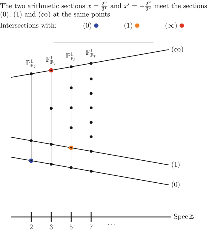

  

  Arithmetic sections are determined by their radicals at 0, 1, ∞ up to finite ambiguity

Remark 3.8

The abc-conjecture implies that there exists only a finite number of triples of coprime integers (a, b, c) such that a + b = c, and rad(abc) ≤ N. This is a special case of the finiteness of solutions of the S-unit equation. It follows, for example, from the weak form of the abc-conjecture proved in [ 44]. This finiteness is due to K. Mahler, originally. See [ 28] and the references therein for more general statements. We illustrate below the case where rad(abc) = 2.3.5 = 30.

Some of the solutions of the equation 2^x ± 3^y = ±5^z are (x, y, z) = (1, 1, 1), (2, 2, 1), (1, 3, 2), (4, 2, 2), (7, 1, 3). It is probably not easy to get a complete list of all solutions, even over ℤ.

3.6 abc Implies Orbifold Mordell

Since this is shown in [26] when Δ = 0, we only need to show this for the remaining ‘minimal’ cases listed in Remark 3.2. We start with ℙ¹ with 3 marked points.

• Let us show that abc implies the Mordell orbifold conjecture over ℚ for (ℙ¹,  Δ) with Δ as in Example 2.7 above. Indeed: if a (resp. b, resp. c) is p-powerful (resp. q-powerful, resp. r-powerful), we have: $rad(a)\leq a^{\frac {1}{p}}\leq c^{\frac {1}{p}}$, and similarly $rad(b)\leq c^{\frac {1}{q}}$, $rad(c)\leq c^{\frac {1}{r}}$. We thus get: $rad(abc)\leq rad(a).rad(b).rad(c)\leq c^{\frac {1}{p}+\frac {1}{q}+\frac {1}{r}}\leq c^{1- \frac {1}{42}}$, since $\frac {1}{p}+\frac {1}{q}+\frac {1}{r}\leq 1-\frac {1}{42}$ for each of the minimal orbifolds listed in Example 2.7, the minimum being reached for the multiplicities (2, 3, 7). The conjecture abc implies that: $c^{1- \frac {1}{42}}\geq rad(abc)\geq \frac {c^{1-\varepsilon }}{C_{\varepsilon }}$, for any ε > 0. Choosing $\varepsilon < \frac {1}{42}$ gives: $c^{ \frac {1}{42}-\varepsilon }\leq C_{\varepsilon }$, and so the claimed finiteness.¹¹

• The Orbifold Mordell conjecture can be deduced from the abc-conjecture also in the three remaining cases when either C = ℙ¹, and Δ is supported by 4 or 5 points on ℙ¹ with multiplicities (2, 2, 2, 3) and (2, 2, 2, 2, 2), respectively, or when C is elliptic and Δ is supported on a single point with multiplicity 2. The derivation is, however, less direct less: one needs to apply a variant of the method used by N. Elkies in [26] to derive Faltings’ theorem from the abc-conjecture. One can proceed as follows:¹²

• First step (the same thus as in [41]):

Let f : C := ℙ¹ → B := ℙ¹ be a rational function $f=\frac {F}{G}$ of degree d > 0, quotient of polynomials F, G, defined over k, a number field. We shall use the notations of [26]. Let P ∈ C(k), such that f(P)∉{0, 1, ∞}. Let H(P) (resp. H _P) be the height of P (resp. of f(P)). We denote by N ₀(f(P)) the radical of F(P). We have: Log(H(f(P))) = d.Log(H(P)) + O(1).

Elkies shows that $Log(N_0(f(P)))\leq (\frac {k_0}{d}). Log(H(P))+O(1)$, where k ₀ is the cardinality (without multiplicities) of f ⁻¹(0). (The proof just consists in removing the ramifications on this fibre). One has then similar inequalities over the fibres of f over 1 and ∞ replacing f by (f − 1) and $\frac {1}{f}$. From which he concludes (using the Riemann–Hurwitz formula) that (k ₀ + k ₁ + k _∞).Log(H(f(P))) ≥ d.Log(N(f(P))) + O(1), with N := N ₀ + N ₁ + N _∞, where N ₁, N _∞ are defined as N ₀, but considering the fibres over 1, ∞ instead of 0.

His argument easily extends to the case where C is equipped with an orbifold divisor Δ supported on the union of the fibres of f over 0, 1, ∞. Let, for each point a _j in this union, m _j be its multiplicity in Δ, and t _j be the order of ramification of f at a _j. Define the number $d_0:=\sum _{a_j\in f^{-1}(0)} (m_j-1).t_j$. Define similarly d ₁, d _∞ for the fibres of f over 1 and ∞. Elkies argument then shows that: k ₀.Log(H(f(P))) ≥ (d + d ₀).Log(N ₀(f(P)) + O(1). Adding the two other inequalities on the fibres of f over 1, ∞, we get:

$$\displaystyle \begin{aligned} (k_0+k_1+k_{\infty}).Log(H(f(P)))\geq (d.Log(N(f(P))+\delta+O(1), \end{aligned}$$

where: δ = d ₀.Log(N ₀(f(P))) + d ₁.Log(N ₁(f(P))) + d _∞.Log(N _∞(f(P)))

Assume now that f is unramified outside of the three fibres over 0, 1, ∞. We then have: (k ₀ + k ₁ + k _∞) = d + 2. Assume also that min{d ₀, d ₁, d _∞}≥ 3.

We obtain: (d + 2).Log(H(f(P))) ≥ (d + 3).Log(N(f(P))), an inequality satisfied only for finitely many P′s ∈ k, by the abc-conjecture. This implies Mordell orbifold for (C,  Δ).

• Second step (construction of Belyi maps):

In order to show that this applies to C = ℙ¹, with Δ either of the form (2, 2, 2, 3) or (2, 2, 2, 2, 2), we consider f : ℙ¹ →ℙ¹ defined by $f(x):=\frac {x^2(x-1)(x-w)}{ux-v}$. The fibre of f over 0 consists thus of 3 points, one double (0), two simple (1, w). The fibre of f over ∞ consists of two points: the triple point ∞ and the single point $\frac {v}{u}$. We now fix 2 further points (distinct from the preceding ones): b, c, and notice that the equation: x ²(x − 1)(x − w) = (ux + v) + (x − b)²(x − c)(x − t) with unknowns u, v, w, t has a unique solution. This means that the fibre of f over 1 has 3 points: one double (b) and two simple ones: (c, t).

In order to deal with Δ = (2, 2, 2, 3), we attribute to the points 0, 1, b, ∞, respectively, the multiplicities 2, 2, 3, 2 . An easy check shows that d ₁ = 4, d ₀ = d _∞ = 3.

In order to deal with Δ = (2, 2, 2, 2, 2), we attribute to all of the 5 points 0, 1, b, c, ∞ the multiplicity 2. One again easily checks that d ₀ = d ₁ = d _∞ = 3.

The last remaining case is when C is elliptic, and $\Delta =(1-\frac {1}{2}).\{a\}, a\in C(k)$. It can be reduced similarly to abc by composing the above map $f(x):=\frac {x^2(x-1)(x-w)}{ux-v}$ with the double cover g : C →ℙ¹ so that its 4 ramification points are sent by f to 0, 1, b, c, and a to ∞, equipping again each of these 5 points with the multiplicity 2.

This concludes the proof that abc implies orbifold Mordell.

3.7 Ramification of Belyi Maps

The question we would like to address here is whether the (non-classical) orbifold Mordell conjecture for one single orbifold pair (ℙ¹,  Δ) of general type: ℙ¹ with the 3 marked points 0, 1, ∞ of multiplicities (3, 3, 4) (for example, one could choose (2, 3, 7) or (2, 4, 5) instead) implies Mordell Conjecture= Faltings’ Theorem, for every curve defined over $\overline {\Bbb Q}$. One may of course raise this question for the other minimal orbifolds over ℙ¹ listed in Remark 3.2.

A positive answer to the following question implies this statement:

Question 3.9

Let C be a curve defined over $\overline {\Bbb Q}$ . Does there exist:

• 1. An unramified cover $u:\tilde {C}\to C$.

• 2. A Belyi map $\beta :\tilde {C}\to \Bbb P^1$ (unramified over the complement of {0, 1, ∞}) such that each of its ramification orders over 0 (resp. 1, resp. ∞) are at least 3, (resp. 3, resp. 4)?

The usual construction of Belyi maps cannot produce Belyi maps such as in the preceding question. Assume indeed that g is already a Belyi map for C, but has some unramified point over each of 0, 1, ∞. In order that f ∘ g be a Belyi map satisfying the condition 2 of 3.9, the map f itself should already be a Belyi map satisfying this very same condition. The Riemann–Hurwitz equality contradicts the existence of such an f.

Faltings’ Theorem would follow from a positive answer to Question 3.9 and Orbifold Mordell. Indeed: fix k, a number field of definition of a given C, and let u, β answering positively the Question 3.9. Let k′∕k be a finite extension such that $u(\tilde {C}(k'))\supset C(k)$ (using the Chevalley–Weil Theorem). Since β is an orbifold morphism to (ℙ¹,  Δ), we get a map with uniformly finite fibres from $\tilde {C}(k')$ to $(\Bbb P^1,\Delta )(\mathcal {O}_{k'})$, the last set being finite by the Orbifold Mordell conjecture for any k′. We thus get the finiteness of C(k).

Remark 3.10

The Question 3.9 bears a certain similarity with the notion of universal curves introduced in [ 7 ] (although the étale covers there are over the universal curve). I thank A. Javanpeykar for bringing this reference to my knowledge.

3.8 Link with Complex Hyperbolicity

Let C be a connected smooth projective curve C. By the Poincaré–Koebe uniformisation, there is a non-constant holomorphic map h : ℂ → C if and only if C is not uniformized by the unit disk 𝔻 ⊂ℂ, that is: if g(C) ≤ 1. Similarly, if C is defined over a number field k, the potential density of C(k) holds if and only if there exists such a map h. It is very easy to check that this equivalence still holds for quasi-projective curves (C − D), again by their uniformisation for the hyperbolic version.

We show in [18], using Nevanlinna’s Second Main Theorem with truncation at order one, that the same thing is true for ‘orbifold curves’ (the notion of morphism h : ℂ → (C,  Δ) being defined as in Definition 2.5 in the two possible ways (‘classical’ and ‘non-classical’). The orbifold Mordell Conjecture thus remains open only in its arithmetic version.

This link, initiated by S. Lang, will be studied in higher dimensions as well.

4 The Kodaira Dimension

4.1 The Iitaka Dimension of a Line Bundle

Since, for projective curves, the invariant h ⁰(C, K _C) = g determines the qualitative arithmetic, it is natural to consider it also in higher dimensions. The invariant h ⁰(X, K _X) is birational, but no longer preserved by étale covers in dimension 2 already, and one needs more information: the values h ⁰(X, m.K _X) := p _m(X), m > 0, the ‘plurigenera’ of Enriques. We shall even abstract more (in order to get a birational invariant preserved by étale covers), and only consider the asymptotic behaviour of the plurigenera as m goes to + ∞, for a given X. The notion actually makes sense, and is extremely useful, more generally, for arbitrary line bundles L, not only for L = K _X.

• Let X be a connected projective manifold of dimension n defined over a field k of characteristic 0. Let L be a line bundle on X. Let h ⁰(X, L) ∈ℕ be the k-dimension of its space H ⁰(X, L) of sections. If h ⁰(X, L) > 0, let be the rational map which sends a generic x ∈ X to the hyperplane of H ⁰(X, L) consisting of sections vanishing at x. We thus have: 0 ≤ dim(Φ _L(X)) ≤ n. We denote either with m.L or with L ^⊗m, m ∈ℤ the m-th power of L.

Definition 4.1

We define κ(X, L) ∈{−∞, 0, …, n} as being −∞ if h ⁰(X, mL) = 0, ∀m > 0. Otherwise, κ(X, L) := max _m>0{dim(Φ _mL(X))}.

An alternative definition, not immediately, equivalent is:

$$\displaystyle \begin{aligned} \kappa(X,L):=\overline{lim}_{m\to +\infty}\big\{\frac{Log h^0(X,m.L)}{Log m}\big\}, \end{aligned}$$

roughly meaning that h ⁰(X, m.L) grows like the κ(X, L)-th power of m as m goes to + ∞.

Example 4.2

• κ(X, L) = −∞ if $L={\mathcal O}_X(-D)$ for some effective divisor D. And also when X is an elliptic curve, if c ₁(L) = 0, but L is not torsion in Pic(X).

• κ(X, L) = 0 iff h ⁰(X, mL) ≤ 1, ∀m > 0, with equality for some m > 0, for example, if L is torsion in Pic(X).

• κ(X, L) = n iff mL = A + E, for some m > 0, A ample and E effective. Then L is said to be ‘big’.

• κ(X, L) = d ∈{1, …., n} if p : X → Z be regular onto, with d := dim(Z), and L = p ^∗(A), A ∈ Pic(Z), ample. Indeed, one has:

• κ(X, p ^∗(M)) = κ(Z, M), for any line bundle M on Z.

The following theorem gives a weak analogue in general:

Theorem 4.3

If κ(X, L) = d ≥ 0, for any sufficiently large and divisible integer m > 0, the rational map Φ _m.L has connected fibres, its image Z _m = Z has dimension d and its generic fibre X _z has $\kappa (X_z,L_{\vert X_z})=0$. Moreover, Z _m is birationally independent of m > 0 sufficiently large and divisible.

If d = n, Φ _mL(X) is birational to X for m large enough.

Observe however that, in general, L will not be torsion on the general fibre of Φ _mL. Many more details and numerous examples can be found in [46].

The following Proposition gives an upper bound on κ(X, L):

Proposition 4.4 (‘Easy Additivity’)

Let p : X → Z be a fibration, and L ∈ Pic(X). Let X _z be the general fibre of p. Then:

$$\displaystyle \begin{aligned} \kappa(X,L)\leq \kappa(X_z,L_{\vert X_z})+dim(Z). \end{aligned}$$

4.2 The Kodaira Dimension κ

The fundamental case is when $L=K_X:=det(\varOmega ^1_X)$, the canonical line bundle on X. One writes then: κ(X) := κ(X, K _X).

The invariant κ(X) enjoys several properties:

• It is birational, and preserved by finite étale covers.

• Additive for products: κ(X := Y × Z) = κ(Y ) + κ(Z), since:

  $$\displaystyle \begin{aligned} h^0(X,mK_X)=h^0(Y,mK_Y)\times h^0(Z,mK_Z),\forall m. \end{aligned}$$

• In particular: κ(X) = −∞, ∀Z, if κ(Y ) = −∞ (e.g.: Y = ℙ¹).

• Also: κ(X) = κ(Z) if κ(Y ) = 0.

4.3 First Examples: Curves and Hypersurfaces

For curves, κ(X) tells (almost) everything, qualitatively, it indeed describes X, its topology, fundamental group, as well as hyperbolicity and arithmetic properties.

κ	g	X	X(k)
−∞	g = 0	ℙ1	Potentially dense
0	g = 1	ℂ∕Λ	Potentially dense
1	g ≥ 2	𝔻∕ Γ	Not potentially dense

The preceding trichotomy (according to the ‘sign’ of K _X: positive, zero or negative) still appears in the special case of smooth hypersurfaces in ℙ_n+1.

• Hypersurfaces in ℙ_n+1. Let H _d ⊂ℙ_n+1 be a smooth hypersurface of degree d (defining by a homogeneous polynomial in (n + 2) variables of degree d). The adjunction formula shows that $K_{H_d}=\mathcal {O}(d-n+2)_{\vert H_d}$. Thus $K_{H_d}$ is ample if d ≥ (n + 3), trivial if d = (n + 2) and anti-ample if d ≤ (n + 1). We thus have, in particular: κ(H _d) = n (resp. 0, resp.−∞) if d > n + 2 (resp. d = n + 2, resp. d < n + 2).

• Hypersurfaces in ℙ_n+1−k ×ℙ_k. Let now $H:=H_{d,d'}$ be a smooth hypersurface of bidegree (d, d′) in this product (this means that H ∩ F is a hypersurface of degree d′ (resp. d) when intersected with a generic ℙ_n+1−k ×{a′} (resp. {a}×ℙ_k). The adjunction formula now shows that $K_H=\mathcal {O}(d-(n+2-k), d'-(k+1))_{\vert H}$. One thus obtains that κ(H) = −∞ if d ≤ n + 1 − k, or if d′≤ k, that κ(H) = 0 if d = n + 2 − k and d′ = k + 1, that κ(H) = k if d = n + 2 − k, d′≥ k + 2, that κ(H) = n + 1 − k if d > n + 2 − k, d′ = k + 1, and that κ(H) = n if d > n + 2 − k, d′ > k + 1.

• The smooth hypersurfaces in products of projective spaces show that arbitrary κ may occur, which are not determined simply by those of base and fibres.

4.4 The Iitaka–Moishezon Fibration

There are 3 fundamental cases (as for curves with g = 0, 1, ≥ 2):

• 1. κ(X) = −∞.

• 2. κ(X) = 0.

• 3. κ(X) = n. In this third case, X is said to be ‘of general type’.

Let us briefly comment on these 3 classes:

• κ = n is a large class (as for curves), it contains the smooth hypersurfaces of degree at least (n + 3) in ℙ_n+1. This is the reason for the term ‘general type’ introduced by B. Moishezon. They are conjectured to be Mordellic by S. Lang. Examples of manifolds of general type are quotients of bounded domains in ℂⁿ by discrete torsion-free groups of automorphisms, which are higher dimensional analogues of curves of genus greater than 1. But many manifolds of general type (such as hypersurfaces of dimension greater than 1) are simply connected.

• κ = 0 contains manifolds with trivial (or torsion) canonical bundle, the structure of which is partially understood by means of the Beauville–Bogomolov–Yau decomposition theorem. They are however classified only in dimension 2. Even in dimension 3, it is unknown whether or not there are finitely many deformation families.

We conjecture that the manifolds with κ = 0 are Potentially Dense. It is expected that on suitable mildly singular birational models their canonical bundle becomes torsion.

• κ = −∞: this class contains products ℙ¹ × Z, ∀Z. It is discussed below.

This class thus does not consist only of Potentially dense manifolds. We define below the more restricted class of ‘rationally connected’ manifolds, conjectured to be potentially dense, which permits to ‘split’ any manifold with κ = −∞ by means of a single fibration into a rationally connected part (the fibres), and a part (conjecturally) with κ ≥ 0 (the base).

• The structure of the intermediate cases when 1 ≤ κ(X) = d ≤ (n − 1) ‘reduces’ (to some extent) to the case of κ = 0 and lower dimension, by means of the following ‘Iitaka–Moishezon fibration’ J.

Proposition 4.5

The map for m > 0 suitably large and divisible is birationally well-defined, and may thus be assumed to be regular. Its generic fibres X _z are then smooth with κ(X _z) = 0, because $\kappa (X_z,K_{X\vert X_z})=0$, and $K_{X\vert X_z}=K_{X_z}$ (by the ‘Adjunction formula’).

J is defined over k, if so is X

Example 4.6

The fibration J is the projection onto the second (resp. first) factor when $H_{d,d'}\subset \Bbb P_{n+1-k}\times \Bbb P_{k}$ is a smooth hypersurface of bidegree (n + 2 − k, d′) (resp. (d, k + 1) if d′ > k + 1 (resp. (d > n + 1 − k)).

When κ(X) = 0, Z is a point, and J does not give any information. In the other extreme case, where κ(X) = n, J embeds birationally X in the projective space ℙ((H ⁰(X, m.K _X)^∗), for appropriate m > 0. One thus ‘reconstructs’ X from its pluricanonical sections.

Caution

In general, however, κ(Z) ≤ d := dim(Z) = κ(X) (and strict inequality may occur, as shown by Example 4.6, since the base of J is then a projective space). The fibration J thus does not in general decompose X in parts with κ(X _z) = 0 and κ(Z) = dim(Z).

• Notice also that J is not defined when κ(X) = −∞. This case κ(X) = −∞ requires a completely different treatment, which we briefly describe below.

4.5 Rational Curves and κ = −∞

In order not to overload the text with quotations, we have deleted them for this section. The results in this section are mainly due to Mori, Miyaoka–Mori, Campana, Kollár–Miyaoka–Mori, Graber–Harris–Starr.

Definition 4.7

A ‘rational curve’ on X is the image of a regular non-constant map: ℙ ¹ → X. We say that X is uniruled if it is covered by rational curves, or equivalently, if there exists a dominant rational map for some (n − 1) dimensional variety T _n−1.

If X is uniruled : κ(X) ≤ κ(ℙ¹ × T) = −∞. Thus κ(X) = −∞. The converse is a central conjecture of birational geometry, known up to dimension 3:

Conjecture 4.8 (‘Uniruledness Conjecture’)

If κ(X) = −∞, X is uniruled.

The decomposition of arbitrary X into parts with a ‘birationally signed’ canonical bundle depends on some or other form of this central conjecture.

4.6 Rational Connectedness and κ ⁺ = −∞

Definition 4.9

X is ‘rationally connected’ (RC for short) if any two generic points of X are joined by a rational curve.

Example 4.10

• 1. Let X = ℙ ¹ × C, for C a projective curve of genus g: X is uniruled, but it is rationally connected if and only if g = 0.

• 2. Unirational manifolds (those dominated by ℙ ⁿ) are RC.

• 3. Fano manifolds (those with − K _X ample) are rationally connected.

• 4. Smooth hypersurfaces of degree at most (n + 1) in ℙ ⁿ⁺¹ are Fano.

• 5. Rationally connected manifolds are simply connected.

• 6. Although no rationally connected manifold is presently proved to be non-unirational, it is expected that this is the case for most rationally connected manifolds of dimension 3 or more. In particular, the (non) unirationality of the double cover of ℙ ₃ ramified along a smooth sextic surface S ₆ is an open problem.

Remark 4.11

If X is defined over a field k ⊂ℂ and is uniruled (resp. rational, unirational, rationally connected over ℂ) it is not difficult to see that it has this property also over some finite extension of k.

Theorem 4.12

For any X, there is a unique fibration r _X : X → R _X such that:

• 1. its fibres are rationally connected, and:

• 2. R _X is not uniruled.

It is called the ‘rational quotient’, or the ‘MRC ¹³ of X.

If X is defined over k, so is r _X.

The fibration r _X thus decomposes X into its antithetic parts: rationally connected (the fibres) and non-uniruled (the base R _X). The extreme cases are when X = R _X (i.e.: X is not uniruled), and when R _X is a point (i.e.: X is rationally connected).

Remark that the uniruledness conjecture implies that κ(R _X) ≥ 0. This leads to the following definition:

Definition 4.13

Define, for any projective X:

From Theorem 4.12, one gets:

Proposition 4.14

Assume the Uniruledness Conjecture 4.8 . The following are then equivalent:

• 1. X is rationally connected.

• 2. κ ⁺(X) = −∞.

Moreover, the ‘rational quotient’ is also the unique fibration g : X → Z on any X such that:

• 1. κ ⁺(X _z) = −∞ for the general fibre X _z of g, and:

• 2. κ(Z) ≥ 0.

Note that these conjectural characterisations of rational connectedness and of r do not rely on rational curves, but only on κ and its refinement κ ⁺. The rational quotient will also be constructed without mentioning rational curves, conditionally on conjecture C _n,m, in §6.5.

Remark 4.15

We conjecture that manifolds with κ ⁺ = −∞ are potentially dense. Thus so should be the rationally connected manifolds. Much more generally, we conjecture that ‘special manifolds’ (defined later) are exactly the potentially dense manifolds.

5 Surfaces

5.1 Classification of Surfaces

If S is a smooth projective surface, we have: κ := κ(S) ∈{−∞, 0, 1, 2}. The maps r and J permit to elucidate the structure of S when κ(S) ≠ 2.

When κ = −∞, the uniruledness conjecture is a classical result of Castelnuovo, and we thus get a non-trivial rational quotient r : S → R, where R is either a curve C _q of genus $q=h^0(S,\varOmega ^1_S)>0$, or a point (in which case S is rationally connected, and even rational).

When κ = 1, one has the Iitaka–Moishezon fibration J : S → B, with smooth fibres elliptic, and B a curve. One says that S is an elliptic surface over B.

When κ = 0, a precise classification is known: S is covered by a blow-up of either an abelian surface or of a K3 surface, where K3-surfaces are defined by: $q=0, K_S\cong \mathcal {O}_S$. They form a single deformation family containing the smooth quartics in ℙ₃.

One thus gets the ‘Enriques–Kodaira–Shafarevich’ classification, displayed in the table below (up to birational equivalence and finite étale covers), where C _q denotes a curve of genus q, $q:=h^0(S,\varOmega ^1_S)=\frac {1}{2}b_1(X)$. We indicate the status of potential density for S defined over some large number field k. More details below.

κ	q	S(up to bir, étale ≅)	S(k) potentially dense
−∞	q ≥ 0	ℙ1 × C q	Yes iff q ≤ 1
0	0	K3	Yes in many examples
0	2	(ℂ2∕Λ)	Yes, always
1	≥ 0	Elliptic over C q	Yes in many examples if q ≤ 1
2	≥ 0	No classification scheme	No, in all known examples

5.2 Remarks on Potential Density

Our guiding principle here consists of the following 3 facts, for X a smooth connected projective manifold defined over a number field k:

• 0. Potential density is a birational property.

• 1. Chevalley–Weil theorem: if X′→ X is an étale covering, X′(k) is potentially dense if X(k) is (the converse is obvious).

• 2. Lang’s conjecture:¹⁴ if X is ‘of general type’, then X(k) is not potentially dense.

By Faltings’ theorem this holds for curves, but is open for surfaces.

Definition 5.1

We say that X (defined over ℂ) is ‘weakly special’ if, for any finite étale cover u : X′→ X, there exists no dominant rational map , with Z of ‘general type’ and dim(Z) > 0.

Remark 5.2

The 3 facts above imply that if X is not weakly special, X(k) is not potentially dense. The following claims the converse also:

Conjecture 5.3 ( [30, Conjecture 1.2])

A projective manifold X∕k is potentially dense if and only if X is ‘weakly special’.

Remark 5.4

This conjecture conflicts with other conjectures stated below ¹⁵ when dim(X) ≥ 3, but both conjectures agree for surfaces (because specialness and weak specialness coincide for them).

Let us check the known cases of this conjecture for surfaces, according to κ(S) = κ, for S a surface defined over a number field k. Let $r:\tilde {S}\to S$ be any finite étale cover of S, and $\tilde {q}(S)$ the supremum (possibly infinite) of $q(\tilde {S})$ when $\tilde {S}$ ranges over all finite étale covers of S. For example, $\tilde {q}(S)=+\infty$ if some $\tilde {S}$ fibres over a curve of genus g ≥ 2. Recall that a Theorem of Y.T. Siu shows that this happens if and only if some finite index subgroup of π ₁(S) admits a quotient which is a ‘surface group’ (i.e.: of the form π ₁(C) with g(C) ≥ 2). Notice that $\tilde {q}(S)\geq 2$ and κ(S) ≠ 0, 2 imply that some $\tilde {S}$ fibres over a curve of genus at least 2, and so that: $\tilde {q}(S)=+\infty$.

• κ = 2. If $\tilde {q}(S)\geq 2$, then S is Mordellic, by Faltings’ Theorem (and Kawamata Theorem on the structure of ramified covers of Abelian varieties) showing that a subvariety of general type of an Abelian variety is Mordellic. If $\tilde {q}(S)=0,1$, S is Mordellic conditionally on Lang’s conjecture.

• κ = −∞. Then S = ℙ¹ × C _q. Thus S(k) is potentially dense if and only if so is C _q: The conjecture is true.

• κ = 0. Some $\tilde {S}$ is either an Abelian surface, or a K3 surface. Both are easily seen to be weakly special. If S is an Abelian surface, S(k) is potentially dense, and the conjecture then holds.

The conjecture then claims that K3 surfaces are potentially dense. This is unknown in general, but known for K3 surfaces which are Kummer, or admit either an elliptic fibration, or an automorphism group of infinite order [6], the main idea of which is: if f : S → C is an elliptic fibration onto the curve C, and if S contains a rational or elliptic ‘non-torsion multisection’, then S(k) is potentially dense.

A ‘non-torsion multisection’ is an irreducible curve D ⊂ C such that f(D) = C, and moreover such that, over the generic point of C, the fibre of D has two points the difference of which is not torsion in the group of translations of this (elliptic) fibre.

It is shown in [6] (this is the hardest geometric part) that elliptic K3 surfaces always contain some rational or elliptic ‘non-torsion’ D.

• κ = 1. Let f : S → C be the (elliptic) Moishezon–Iitaka fibration. A major rôle is played by the ‘multiple fibres’ of f. Let indeed, for s ∈ C, f ^∗(s) := (∑_ht _h.F _h) be the scheme-theoretic fibre of f over s. Define: m _s := gcd _h{t _h}. This is the ‘classical’ multiplicity¹⁶ of the fibre of f over s, and it is equal to 1, except for finitely many (possibly none) s ∈ C. We define now the ‘orbifold base of f’ to be the orbifold curve (C, Δ_f), with $\Delta _f:=\sum _{s\in C} (1-\frac {1}{m_s}).\{s\}$, a finite sum since $(1-\frac {1}{m_s})=0$ iff m _s = 1.

In this situation, we now have the following (geometric):

Lemma 5.5

An elliptic projective smooth surface S is weakly special if and only if deg(K _C + Δ _f) ≤ 0.

Proof

The proof has two steps. First step: show that there exists¹⁷ an ‘orbifold-étale’ cover u : C′→ C over Δ_f. Then $K_{C'}=u^*(K_C+\Delta _f),$ so that $deg(K_{C'})\leq 0$ iff deg(K _C + Δ_f) ≤ 0.

Second step: the (normalised) base-change $f':S':=\widehat {S\times _CC'}\to C'$ has the property that u : S′→ S is étale.

If deg(K _C + Δ_f) > 0, g(C′) ≥ 2, and S is not weakly special in this case. Notice that Faltings’ and Chevalley–Weil theorems imply that S(k) is not potentially dense, and the conjecture is true unconditionally.

If deg(K _C + Δ_f) ≤ 0, C′ is rational or elliptic, and since f′ : S′→ C′ has no multiple fibre, there is an exact sequence of groups:

$$\displaystyle \begin{aligned} \pi_1(F^{\prime}_s)\to \pi_1(S')\to \pi_1(C')\to \{1\}\end{aligned}$$

which implies that no étale cover of S′ has a fibration onto a curve C″ with g(C″) ≥ 2 (since π ₁(C″) has the free group on 2 generators as a quotient, and is not solvable). □

The Conjecture 5.3 is thus equivalent to the fact that S(k′) is dense when deg(K _C + Δ_f) ≤ 0, which is open, but verified on many examples.

5.3 Fibred Simply Connected Surfaces of General Type

We shall give here examples of smooth projective simply connected surfaces S of general type (defined over ℚ) which are not potentially dense, conditionally on the Orbifold Mordell Conjecture.¹⁸ Presently (July 2019) no such example is known unconditionally.¹⁹

Let f : S → C be a fibration (with connected fibres) from the smooth connected projective surface S onto the smooth projective curve C. We do not assume that the smooth fibres are elliptic.

Let s ∈ C, and f ^∗(s) :=∑_ht _h.F _h be the scheme-theoretic fibre of f over s. We define two notions of multiplicity for this fibre:

• The ‘classical’ (or ‘gcd’) multiplicity $m_s^*(f):=gcd_{h}\{t_h\}$.

• The ‘inf’ multiplicity m _s(f) := inf _h{t _h}.

Of course, $m_s^*(f)$ divides m _s(f), both are 1 except possibly on the finite set of singular fibres.

We now define two ‘orbifold bases’ of f:

• The ‘classical’ orbifold base $(C,\Delta ^*_f),$ with $\Delta _f^*:=\sum _{s\in C} (1-\frac {1}{m_s^*(f)}).\{s\}$

• The orbifold base (C, Δ_f), with $\Delta _f:=\sum _{s\in C} (1-\frac {1}{m_s(f)}).\{s\}$

Remark 5.6

• 1. If f is an elliptic fibration, $\Delta _f=\Delta ^*_f$. As we shall see, they may differ, but only if the smooth fibres of f have g ≥ 2.

• 2. If $(C,\Delta ^*_f)$ is of general type, there is always a base-change v : C′→ C, orbifold-étale over $\Delta ^*_f$, with g(C′) ≥ 2, such that the resulting normalised base-change u : S′→ S is étale. Thus π ₁(S′), which is a finite index subgroup of π ₁(S), maps onto π ₁(C′), showing that π ₁(S) is a ‘big’ hyperbolic non-abelian group.

• 3. The map f induces natural group-morphisms $f_*:\pi _1(S)\to \pi _1(C,\Delta ^*_f)$ and $\pi _1(C,\Delta _f)\to \pi _1(C,\Delta ^*_f)$, but f _∗ does not lift to a natural group-morphism π ₁(S) → π ₁(C, Δ _f). Here $\pi _1(C,\Delta ^*_f)$ is the quotient of $\pi _1(S\setminus \Delta ^*_f)$ by the normal subgroup generated by the m _j-th powers of a small loop winding once around D _j, this for any j if $\Delta ^*_f:=\sum _j(1-\frac {1}{m_j}).\{a_j\}$.

We shall now construct fibrations f : S → C with (non-classical) orbifold base (C, Δ_f) of general type with S simply connected.

Proposition 5.7 ( [13])

Let f : S → C be a fibration from the smooth projective connected surface S onto the projective curve C. Assume that deg(K _C + Δ _f) > 0, and that S is simply connected. Then:

• 1. κ(S) = 2, the smooth fibres of f have g ≥ 2.

• 2. There exist such fibrations defined over ℚ. In this case:

• 3. If the orbifold Mordell conjecture is true, then S(k) is contained in a finite number of fibres of f, for any number field k, and S(ℚ) is not potentially dense.

Proof

Claim 1 follows from an ‘orbifold’ version of the C _n,m conjecture (see below). We shall give examples of claim 2 below. For Claim 3, it suffices to see that f(S(k)) is contained in (S, Δ_f)(C) (finite by the orbifold Mordell conjecture) for any k and a sufficiently large finite subset S of the places of k, determined by a ‘model’ of (C, Δ_f) over $\mathcal {O}_{S,k}$, such that (C, Δ_f) has good reduction outside of S. Let thus x ∈ S(k), and t be a k-rational function which gives a local coordinate on C at f(x). Let $\frak {p}$ be a place of k outside S. Assume that x∉f ⁻¹(s), if s is in the support of Δ_f. If the $\frak {p}$ reduction of x belongs to the $\frak {p}$ reduction $(F_h)_{\frak {p}}$of some component F _h of f ⁻¹(s), let t _h be the multiplicity of F _h in f ^∗(s). Then t _h ≥ m _s(f), by definition of m _s(f). On the other hand, the arithmetic intersection number of $f(x)_{\frak {p}}$ with $(s)_{\frak {p}}$ is the product of t _h with the arithmetic intersection number of $(x)_{\frak {p}}$ with $(F_h)_{\frak {p}}$, and is thus a multiple of t _h, and thus at least m _s(f). □

Remark 5.8

In the quasi-projective case, Corvaja–Zannier have given the first example of simply connected quasi-projective smooth surfaces with a non-Zariski dense set of integral points over any number field (see [ 24]). Their proof uses Schmidts’ subspace theorem. Their examples (blow-ups of ℙ ₂ on union of 4 lines, removing the strict transforms, not the total transform, of these lines, which permit to realise the simple-connectedness of the complement) are similar to the ones given in § 8.7 below, using infinite multiplicities, instead of finite ones.

Example 5.9

We now give some examples of fibrations f : S →ℙ ¹ with orbifold base of general type, and S simply connected. Different examples where initially constructed in [ 13]. They are quite complicated, with fibres of high genus g = 13 (but relatively simple multiple fibres consisting of 5 rational curves meeting transversally in a single point, their multiplicities being (2, 2, 2, 3, 3)). In [ 45], L. Stoppino used former work of Namikawa–Ueno [ 38] to give much simpler explicit examples with fibres of (minimal possible) genus 2. In these examples, as in the examples produced in [ 13], the ‘non-classical’ multiple fibres have ‘inf’-multiplicity 2. We describe here the simplest example of [ 41], to which we refer for more details, and in particular the (quite involved) description of the multiple fibres, which are trees of rational curves (and so are simply connected) (Figure 4).

Fig. 4

A non-classical double fibre of genus 2

• Take the ramified 2-cover π ₀ : S ₀ →ℙ ¹ ×ℙ ¹ of equation y ² = t(x ⁶ + t.x ³ + t ²) (with affine coordinates (t, x) on ℙ ¹ ×ℙ ¹). Resolve by r : S → S ₀ the singularities of S ₀ to get an isotrivial fibration f = q ∘ π ₀ ∘ r : S →ℙ ¹, where q : ℙ ¹ ×ℙ ¹ →ℙ ¹ is the first projection which sends (t, x) to t. The fibration has then smooth fibres of genus 2 and two simply connected fibres of ‘inf’-multiplicity 2, over t = 0, ∞. More precisely, each of these fibres consists of 6 rational curves building a tree, their multiplicities being (2, 6, 3, 3, 4, 2).

• The surface S so constructed is defined over ℚ, and is rational. It is thus potentially dense. In order to get a fibration of general type, it is sufficient to make a generic cyclic base-change u : ℙ ¹ →ℙ ¹ of degree d ≥ 3 over the base of q, and to normalise. The resulting surface S′ is then of general type, simply connected, defined over ℚ, and the resulting fibration f′ : S′→ℙ ¹ has 2d ≥ 6 ‘non-classical’ double fibres, and no ‘classical’ multiple fibre. The ‘orbifold Mordell Conjecture’ then implies that it is not potentially dense. This would provide the first non-potentially dense simply connected smooth surface defined over a number field.

5.4 Link with Hyperbolicity

• In [18], Corollary 4, p. 208, based on Nevanlinna’s second main theorem with truncation at level 1, it is shown that any entire curve h : ℂ → S has its image contained in a rational or elliptic component of some singular fibre of f, if S has a fibration on a curve such that its orbifold base is of general type. This is the exact hyperbolicity analog of the conjectural arithmetic statement of non-potential density.

• It is shown in [10] that a complex projective surface S not of general type admits a holomorphic map h : ℂ² → S with dense image, if and only if S is weakly special (with the possible exception of non-elliptic and non-Kummer K3 surfaces). This leads to conjecture the equivalence of the following three properties:

  • 1. S is weakly special

  • 2. S admit a dense entire curve²⁰

  • 3. S(k) is potentially dense (if S is defined over a number field k).

• Insufficiencies of the ‘weak specialness’: We shall see in §8.7 that from dimension 3 on, the property of ‘weak specialness’ is too weak to imply property 2 (and conjecturally also property 3) above. We shall replace it by the ‘specialness’ property, defined below.

6 Decomposition of Arbitrary X’s

We have previously defined 3 classes of ‘primitive’ manifolds: those with κ ⁺ = −∞, κ = 0, or with κ = dim (i.e.: of general type), respective generalisations of rational, elliptic, and hyperbolic curves. We now decompose any higher dimensional X into ‘twisted products’ of manifolds of these 3 primitive types by a suitable sequence of canonical and (birationally) functorial fibrations. We first describe a decomposition by a canonically defined sequence of fibrations, which is however conditional in the uniruledness Conjecture 4.8. We next define a second decomposition by one single fibration which is unconditional and also birationally functorial (while the steps of the first are not). The abutments of both decompositions however agree (the first one existing only conditionally).

6.1 The (J ∘ r)ⁿ Decomposition

Let X be arbitrarily be given, and let r : X → R _X be its ‘rational quotient’. Assuming the ‘uniruledness Conjecture’ 4.8, one gets that κ(R _X) ≥ 0, so that the Iitaka–Moishezon fibration J : R _X → J(R _X) is always birationally defined.²¹ The composite map: J ∘ r : X → J(R _X) is thus defined for every X, and can be iterated. The following properties are easy:

• 1. X = J(R _X) if and only if X is of general type. Thus:

• 2. Defining inductively the k-th iterate $(J\circ r)^k:X\to X_k=(J(R_{X_{k-1}}))$, with X ₀ := X, we see that d _k := dim(X _k) is decreasing. Next (by 1.), d _k+1 = d _k if and only if X _k is of general type.

• 3. In particular, (J ∘ r)ⁿ : X → X _n is a fibration over a manifold X _n of general type (possibly a point), with fibres towers of fibrations with fibres alternatively either rationally connected, or with κ = 0.

We call this map c : (J ∘ r)ⁿ : X → X _n the ‘weak core map’ of X. It has been constructed conditionally on Conjecture 4.8. We shall now give a (more general) unconditional construction.

The ‘weak core map’ however fails to be preserved even by finite étale covers (see Example 6.15). This is due to neglecting the multiple fibres of the fibrations J. This will be corrected later (see §8.1) by introducing ‘orbifold bases’ of fibrations.

The relevance to potential density will be explained in §8.4.

6.2 The C _n,m Conjecture

Let f : X → Z be a fibration between complex projective manifolds, denote by X _z its generic (smooth) fibre.

Proposition 6.1 (‘Easy Addition’)

κ(X) ≤ κ(X _z) + dim(Z).²²

The following is a central conjecture of classification:

Conjecture 6.2 (‘C _n,m-conjecture’)

κ(X) ≥ κ(X _z) + κ(Z).

Theorem 6.3 (E. Viehweg)

κ(X) = κ(X _z) + dim(Z) when Z is of general type. In particular, if X _z is of general type, so is X.

We shall formulate an ‘orbifold’ version of this conjecture in §7.4. This orbifold version is known also when the ‘orbifold base’ of f is of general type.

Corollary 6.4

If κ(X) = 0, there is no rational fibration f : X → Z, with Z of general type and dim(Z) > 0.

Indeed: 0 = κ(X) ≥ κ(X _z) + dim(Z) > κ(X _z) ≥ 0 (the last inequality is easy).

6.3 A Decomposition Criterion

Let $\mathcal {C}$ be a class of complex (connected) projective manifolds, stable by birational equivalence. We denote by $\mathcal {C}^{\perp }$ the class of all (complex projective) manifolds X which do not admit any dominant rational fibration onto any $Z\in \mathcal {C}$. We call $\mathcal {C}^{\perp }$ the ‘Kernel’ of $\mathcal {C}$.

Definition 6.5

We say that the class $\mathcal {C}$ is ‘stable’ if the following two properties E1 and E2 hold true.

(E1) If f : X → Z is a surjective regular fibration with general (smooth) fibre $X_z\in \mathcal {C}$, and $Z\in \mathcal {C}$. Then $X\in \mathcal {C}$.

(E2) If a connected projective manifold Y  is equipped with two (surjective) fibrations h : Y → Z, g : Y → T such that h : Y _t → h(Y _t) ⊂ Z is birational for t ∈ T generic, and if $Z\in \mathcal {C},$ then $Y_t \in \mathcal {C}$ for t ∈ T generic. We abbreviate this property by saying that the general member of a Z-covering family of varieties is in $\mathcal {C}$ if $Z\in \mathcal {C}$.

Theorem 6.6

Assume that $\mathcal {C}$ is stable. Then, for any complex projective X, there exists a unique fibration γ _X : X → C _X such that:

• 1. its general fibre $X_z\in \mathcal {C}^{\perp }$.

• 2. $C_X\in \mathcal {C}$.

If X is defined over k, so is γ _X.

We call γ _X the $\mathcal {C}$ -splitting of X.

The $\mathcal {C}$-splitting is functorial: any rational dominant fibration f : X → Z induces a unique rational fibration γ _f : C _X → C _Z such that γ _Z ∘ f = γ _f ∘ γ _X.

Proof

We proceed by induction on n := dim(X), the assertion being true for n = 0 (in which case $X\in \mathcal {C}\cap \mathcal {C}^{\perp }$, by convention). Let g : X → Z be a rational fibration with $Z\in \mathcal {C}$, d := dim(Z) being maximal with this property. If d = 0, we are finished since then $X\in \mathcal {C}^{\perp }$, by definition. Otherwise: (n − d) > 0, and so the proposition holds for X _z. By uniqueness of the map γ for X _z, Chow space theory shows the existence of fibration γ _X∕Z : X → Y  and h : Y → Z such that h ∘ γ _X∕Z = g, and such that the restriction γ _z : X _z → Y _z is $\gamma _{X_z}$ (already inductively existing) for X _z, z ∈ Z general. By property (E1), since we have: $Y_z\in \mathcal {C}$, and $Z\in \mathcal {C}$, we have $Y\in \mathcal {C}$. The maximality of dim(Z) implies that Y = Z, the fibres X _z of g thus coincide with those of γ _X∕Z, which are in $\mathcal {C}^{\perp }$. The map g thus enjoys the two claimed properties.

The uniqueness follows from (E2). Let indeed k : X → Y  be a second fibration enjoying properties 1 and 2, with dim(Y ) maximal, thus dim(Y ) = dim(Z) = d. Let y ∈ Y  be general, X _y := k ⁻¹(y), and Z _y := g(X _y) ⊂ Z. By property E2, $Z_y\in \mathcal {C}$. Since $X_y\in \mathcal {C}^{\perp }$, Z _y is a point. There thus exists a map h : Y → Z such that g = h ∘ k. Since dim(Y ) = dim(Z), we have Z = Y, g = k (birationally).

The functoriality follows from a similar argument: the fibres of γ _X, which are in $\mathcal {C}^{\perp }$, are mapped by γ _Z ∘ f to a covering family of subvarieties of $C_Z\in \mathcal {C}$; they are thus points, by E2. This implies the claimed factorisation of γ _Z ∘ f through γ _X. □

Remark 6.7

The existence of γ _X follows from E1, the uniqueness from E2. The proof shows that the fibres of γ _X are the largest subvarieties of X in $\mathcal {C}^{\perp }$, and that Z = C _X dominates any member of $\mathcal {C}$ dominated by X.

Denoting with $\mathcal {P}$ the class of all (complex, connected) projective manifolds, it is tempting to write the content of the $\mathcal {C}$ -splitting in the form of a short exact sequence $[\mathcal {C}^{\perp }]\to \mathcal {P}\to \mathcal {C}$ , to mean that any $X\in \mathcal {P}$ is in a unique way an ‘extension’ of an element of $\mathcal {C}$ by a (deformation class) of $\mathcal {C}^{\perp }$ , a fibration being seen as an ‘extension’ of its base by its general fibre.

We shall now apply this criterion in two situations.

6.4 The Weak Core Map

Proposition 6.8

Let $\mathcal {C}:=\mathcal {K}^{max}$ be the class of manifolds of general type. It is stable, i.e. enjoys the properties E1,E2 of Theorem 6.6.

Proof

Property E1 follows directly from Theorem 6.3. Property E2 follows from the ‘easy addition’ property (6.1). □

Let now $\mathcal {S}^w$ be the smallest class of complex projective manifolds containing those with κ = 0, κ ⁺ = −∞, and stable by ‘extensions’ (i.e.: such that $X\in \mathcal {S}^w$ whenever there is a fibration f : X → Z with $Z\in \mathcal {S}^w$ and $X_z\in \mathcal {S}^w$).

Lemma 6.9

$\mathcal {S}^w\subset (\mathcal {K}^{max})^{\perp }$ , the class of manifolds not dominating any positive-dimensional manifold of general type.

Proof

$(\mathcal {K}^{max})^{\perp }$ is clearly stable by extensions, and contains the manifolds with κ ⁺ = −∞, by definition. It also contains those with κ = 0, by Corollary 6.4. □

Corollary 6.10

Let c _X : X _n → C _X be the ‘weak core map’ of an arbitrary n-dimensional X = X _n. Assume Conjecture 4.8, so that the map (J ∘ r)ⁿ is defined. Then c _X = (J ∘ r)ⁿ, and $\mathcal {S}^w=(\mathcal {K}^{max})^{\perp }$.

The weak core map is functorial: any fibration f : X → Z induces a (rational, dominant) map c _f : C _X → C _Z.

Proof

Both maps have a base in $\mathcal {K}^{max}$ and general fibres in $(\mathcal {K}^{max})^{\perp }$, they thus coincide by uniqueness of the weak core. Applying this to any $X\in (\mathcal {K}^{max})^{\perp }$ shows that $X\in \mathcal {S}^w$. The functoriality is a special case of Theorem 6.6. □

Remark 6.11

Let us stress that the weak core map is defined unconditionally, contrary to (J ∘ r)ⁿ. Also, the map J is not functorial, and so the functoriality of (J ∘ r)ⁿ does not follow directly from its construction.

6.5 The κ-Rational Quotient

We show here how to construct the rational quotient map r _X : X → R _X without mentioning rational curves (but assuming C _n,m and 4.8).

Let $\mathcal {K}_{\geq 0}$ be the class of projective manifolds X with κ(X) ≥ 0. The class $(\mathcal {K}_{\geq 0})^{\perp }$ thus consists, by definition, of all manifolds with κ ⁺ = −∞.

Lemma 6.12

Assume Conjecture C _n,m. The class $\mathcal {K}_{\geq 0}$ then enjoys properties E1, E2 of Theorem 6.6.

Proof

Property E1 follows directly from C _n,m, property E2 is shown as for the class $\mathcal {K}^{max}$ (by ‘easy addition’). □

Applying Theorem 6.6 and the same argument as in Corollary 6.10, we get:

Proposition 6.13

Assume conjecture C _n,m. For any X, there is a unique fibration ρ _X : X → R(X) such that:

• 1. κ ⁺(X _z) = −∞ for its general fibre X _z, and:

• 2. κ(R(X)) ≥ 0.

We call ρ _X the ‘κ-rational quotient’ of X.

Remark 6.14

We cannot however here show that ρ _X coincides with the ‘true’ rational quotient r _X : X → R _X, because we do not know whether all manifolds with κ ⁺ = −∞ are rationally connected. We can only show (assuming C _n,m) that we have a factorisation φ : R _X → R(X) such that ρ _X = φ ∘ r _X. The fibres of ρ _X are indeed not uniruled with κ ⁺ = −∞. The Conjecture 4.8 thus implies that ρ _X = r _X.

6.6 The Weak Core Is Not Preserved by étale Covers

This is shown by the following (simplest possible) example. This implies (among other things) that it is inappropriate for the description of X(k′). We shall replace it later with the ‘true’ core map, which takes into account the multiple fibres of fibrations, and is preserved by finite étale covers.

Example 6.15

Let C be a hyperelliptic curve of genus g ≥ 2, h : C →ℙ ¹ := C∕ < τ >  be the double cover induced by the hyperelliptic involution τ of C. Let E be an elliptic curve, and t a translation of order 2 on E. Let S′ := E × C, and ι := t × τ the fixed-point free involution on S′. Let u : S′→ S be the quotient by ι.

The projections J : S →ℙ ¹ := C∕ < τ >  (resp. J′ : S′→ C) are the Iitaka fibrations of S, S′, and J ∘ u = h ∘ J′. The weak core map c _S := (J ∘ r)² : S → C _S of S maps S to a point, but $c_{S'}=(J\circ r)^2:S'\to C_{S'}=C$ is simply the fibration J′ : S′→ C, since g(C′) ≥ 2. The natural map $c_u:C_{S'}\to C_S$ thus does not preserve the dimension.

The surface S has an ‘orbifold quotient’ of general type, revealed on its double cover S′, but may be seen directly on S if one considers the ‘orbifold base’ of J, which is indeed of general type.

The ‘orbifold base’ of J consists of the base B = ℙ ¹ := C∕ < τ >  of J, in which the points p _j over which the fibre is multiple (here double) are equipped with the multiplicity (2, here) of the corresponding fibre. The points p _j are here obviously the 2g + 2 points images of the hyperelliptic points of C. We obtain thus the ‘orbifold base’ (B,  Δ) with $\Delta =\sum _{j=1}^{j=2g+2}(1-\frac {1}{2}).\{j\}$, in such a way that h ^∗(K _B +  Δ) = K _C, by the ramification formula. Which indeed shows that the orbifold curve (B,  Δ) is of general type.

A second way to see this quotient of general type is to consider not only the line bundle $J^*(K_{\Bbb P^1})$, but its saturation L _J in $\varOmega ^1_S$, which has κ = 1 (See Example 7.8). As we shall see in Theorem 7.6, the two aspects (orbifold base, saturation of f ^∗(K _S)) actually coincide.

• The failure of the weak core map will be corrected by the introduction of ‘orbifold base’ of fibrations, as in the preceding example. One has then, however, to work in the larger category of ‘orbifold pairs’. Even if one only wants to decompose projective manifolds without orbifold structures, these will appear, as in the preceding example, in general when considering the Moishezon–Iitaka fibration. For surfaces, this can be dealt with by suitable étale covers, but no longer in dimension 3 or more (see Example in §8.7 below).

7 Special Manifolds

7.1 Definition, First Examples and Properties

From now on, X _n is a smooth and connected complex projective manifold²³ of dimension n. Our exposition here is very sketchy. Details can be found in [11] and [13].

Definition 7.1

X is special ²⁴ if κ(X, L) < p for any line bundle $L\subset \varOmega ^p_X$, and for any p > 0.

Example 7.2

• 1. If X is a curve, the unique p > 0 to consider is p = 1, and so $L=K_X=\varOmega ^1_X$. A curve is thus special if either rational or elliptic.

• 2. If X is rationally connected, it is special (since it satisfies the much stronger vanishing: $h^0(X, \otimes ^m\varOmega ^1_X)=0, \forall m>0)$ . This generalises rational curves.

• 3. If κ(X) = 0, X is special. (See 7.11 below). This generalises elliptic curves. Much more is expected to be true: κ(X, L) ≤ 0 for any $L\subset \otimes ^m(\varOmega ^1_X), \forall m>0$, L of rank 1, if κ(X) = 0.

• 4. If X is of general type, it is not special, using $L=K_X=\varOmega ^n_X$.

• 5. More generally: if there is a fibration , with p = dim(Z) > 0, and if Z is of general type, then X is not special (take $L=f^*(K_Z)=f^*(\varOmega ^p_Z)\subset \varOmega ^p_X)$, then κ(X, L) = κ(Z, K _Z) = p, contradicting the specialness of X).

• 6. Being special is preserved by birational equivalence and finite étale covers. Thus ‘special’ implies ‘weakly special’. The converse holds for curves and surfaces, but no longer for threefolds (see § 8.7 below). See Theorem 7.4 for a characterisation of specialness in this direction.

• 7. The Kodaira dimension does not characterise (non-)specialness (except for k = 0, n): if n ≥ 1, k ∈{−∞, 1, …, (n − 1)}, there exist both special and non-special manifolds with dim = n, κ = k.

  Non-special examples are given by obvious products.

  ‘Special’ examples are given, if k ≥ 0, by smooth divisors X in ℙ ^n−k+1 ×ℙ ^k of bidegree (n − k + 2, k + 2).

• 8. If is a meromorphic (possibly transcendental) non-degenerate map, X is special. ‘Non-degenerate’ means that it has non-vanishing Jacobian generically. This is an orbifold version of a result of Kobayashi–Ochiai.

• 9. If S is a smooth projective weakly special surface, it is special. When κ(S) = −∞, 0, it is easy from the classification and 7.11. When κ(S) = 1, this follows from Lemma 5.5.

  Special surfaces thus have a very simple characterisation: κ(S) ≤ 1, and $\tilde {q}(S)\leq 2$. Specialness is preserved by deformation (and even diffeomorphism) for surfaces.

  We conjecture that specialness is preserved by deformations and specialisation of smooth (compact Kähler) manifolds.

Remark 7.3

One could replace the condition κ(X, L) < p by the stronger condition ν(X, L) < p for any rank-one $L\subset \varOmega ^p_X$, where ν(X, L) ≥ κ(X, L) is the numerical dimension of L. It is an open question whether one obtains the same class of manifolds. It has been shown by C. Mourougane and S. Boucksom that ν(X, L) ≤ p, ∀p, L, X, strengthening Bogomolov’s theorem. Notice however that it may happen that κ(X, L) = −∞ if ν(X, L) = p for $L\subset \varOmega ^p_X$, as observed by Brunella on surfaces covered by the bidisk. The situation is similar to the one considered in the next § 7.2.

7.2 The Birational Stability of the Cotangent Bundle

Let X be a complex connected projective manifold.

The canonical algebra K(X) := ⊕_m≥0H ⁰(X, m.K _X), and so also κ(X) are not (birationally) functorial in the sense that a dominant rational map f : X → Z does not induce any natural (injective) morphism of algebras f ^∗ : K(Z) → K(X), or inequality κ(X) ≥ κ(Z) when dim(X) > dim(Z).

The ‘cotangent algebra’ $\varOmega (X):=\oplus _{m\geq 0} H^0(X, \otimes ^m\varOmega ^1_X)$ is, by contrast, obviously functorial, as well as $\kappa ^{++}(X):=max\{\kappa (X,L)\vert L\subset (\otimes ^m \varOmega ^1_X)$ coherent of rank 1, ∀m > 0}. We obviously have: κ ⁺⁺ ≥ κ ⁺ ≥ κ, where κ ⁺ is defined in 4.13, and also obviously functorial.

One can show²⁵ that κ ⁺⁺(X) = κ ⁺⁺(R _X), where r _X : X → R _X is the rational quotient of X (the same holds easily for κ ⁺). This permits to reduce the study of κ ⁺⁺ to the case when K _X is pseudo-effective (i.e.: X not uniruled). Assuming Conjecture 4.8, one even reduces the study of κ ⁺⁺ to the case when κ(X) ≥ 0.

A stronger version is obtained by replacing κ(X, L) by its ‘numerical’ version ν(X, L) ∈{−∞, 0, 1, …, dim(X)} (as defined by N. Nakayama):

$$\displaystyle \begin{aligned} \nu(X,L):=inf \{k\in \Bbb Z\vert \overline{lim}_{m\to +\infty}\big(\frac{h^0(X,mL+A)}{m^k}\big)>0\}, \end{aligned}$$

where A is a sufficiently ample line bundle on X, for example: K _X + (2n + 2).H, H any ample line bundle on X. We have: ν(X, L) ≥ κ(X, L) for any line bundle L on X.

We defined (in [17]) ν ⁺(X) just as κ ⁺⁺(X), just replacing there κ by ν, and showed that ν ⁺(X) = ν(X, K _X) when K _X is pseudo-effective. This is the ‘birational stability’ of the cotangent bundle: the positivity of its line subsheaves is controlled by the canonical bundle (and similarly for its tensor powers) when X is not uniruled.

If we now assume the conjecture that ν(X, K _X) = κ(X) for any X such that K _X is pseudo-effective, we obtain in this case: ν ⁺(X) = ν(X) = κ ⁺⁺(X) = κ(X), and ν ⁺(X) = κ ⁺⁺(X) = κ(R _X) for any X. A particularly important case is when κ(X) = 0, in which case the conjecture is that ν(X) = 0, implying that ν ⁺(X) = κ ⁺⁺(X) = 0, a statement considerably stronger than the proved specialness.

Another consequence of the conjecture ν(X) = κ(X) for X non-uniruled were that κ(X) ≥ κ(Z) for any dominant rational map f : X → Z between non-uniruled manifolds: apply the equality ν ⁺⁺ = ν of [17] to X and Z together with the equalities ν ⁺⁺ = κ ⁺ implied by the conjecture, and the obvious inequality κ ⁺(X) ≥ κ ⁺(Z).

Similar results and conjectures hold for smooth orbifold pairs (X,  Δ) as well (see [17], [14]). When Δ is reduced, one just has to consider $\varOmega ^1_X(Log(\Delta ))$ in place of $\varOmega ^1_X$.

Let us finally observe that the rate of growth of the spaces of sections of the symmetric powers of the cotangent bundle is in general unrelated to the ‘Kodaira’ dimension, as shown by the smooth hypersurfaces of the projective spaces (since their cotangent bundles are known to be non-pseudo-effective).

7.3 Specialness as Opposed to Base Orbifolds of General Type

The following is due to F. Bogomolov:

Theorem 7.4 ( [4])

Let X be projective smooth, and $L\subset \varOmega ^p_X$ a line bundle. Then:

• 1. κ(X, L) ≤ p.

• 2. If κ(X, L) = p, there exists a fibration such that L = f ^∗(K _Z) generically ²⁶ on X.

Line bundles as in 2) are called ‘Bogomolov sheaves’.

Remark 7.5

• 1. Bogomolov sheaves are thus ‘maximally big’ line subsheaves of $\varOmega ^{\bullet }_X$ . And X is special if $\varOmega _X^{\bullet }$ does not contain such maximally big line subsheaves.

• 2. There are many examples of Bogomolov sheaves $L=f^*(K_Z)\subset \varOmega ^p_X$, generically over Z, and such that κ(Z) = −∞. This is due to the multiple fibres of f, encoded in the ‘orbifold base of f’. Hence the geometric characterisation of ‘specialness’ is given in 7.7.

Theorem 7.6

Let f : X → Z _p = Z be a fibration. ²⁷Let $L:=f^*(K_Z)^{sat}\subset \varOmega ^p_X$ be the saturation ²⁸ of f ^∗(K _Z) in $\varOmega ^p_X$.

Then: κ(X, L) = κ(Z, K _Z + Δ _f).²⁹

Thus Δ_f encodes the difference between f ^∗(K _Z) and its saturation: κ(X, f ^∗(K _Z)^sat) − κ(X, f ^∗(K _Z)) = κ(Z, K _Z + Δ_f) − κ(Z, K _Z). This fails for the ‘classical’ orbifold base of f, and is the main reason for the introduction of this ‘non-classical’ notion.

We thus get a geometric characterisation of ‘specialness’:

Corollary 7.7

X is special if and only if, for any fibration , the orbifold base of any of its ‘neat models’ is not of general type.

Of course, this implies that (but turns out to be much stronger than) the non-existence of fibrations with Z of general type.

Example 7.8

Let us give the concrete meaning of the saturation in a simple example: let f : S → C be a fibration of the surface S onto the curve C, with an irreducible smooth fibre F = f ⁻¹(s) of multiplicity t > 1, thus given in local analytic coordinates (x, y)on S by: f(x, y) = u := x ^t. Then $\Delta _f=(1-\frac {1}{t}).\{s\}+\ldots$ near s in C.

Thus f ^∗(K _C) = f ^∗(du) = t.x ^t−1.dx near s, while: $f^*(K_Z+\Delta _f)=f^*\Big (\frac {du}{u^{(1-\frac {1}{t})}}\Big )=t.dx$, which is indeed the saturation of f ^∗(du) in $\varOmega ^1_S$.

7.4 The Orbifold Version of the C _n,m Conjecture

Conjecture 7.9 (Conjecture $C_{n,m}^{orb}$)

Let f : X → Z be a fibration, with generic fibre X _z. Then κ(X) ≥ κ(X _z) + κ(Z, Δ _f).

Without Δ_f, this conjecture is due to S. Iitaka. More general versions³⁰ exist. The special case where (Z, Δ_f) is of general type is known:

Theorem 7.10 (Viehweg)

In the situation of 7.9, if κ(Z, Δ _f) = dim(Z), we have: κ(X) = κ(X _z) + dim(Z).

This result is due to Viehweg when Δ_f = 0. The proof extends with some adaptations to cover this more general case. The range of applicability is considerably extended by the adjunction of the orbifold term.

Corollary 7.11

X is special if κ(X) = 0.

Proof

0 = κ(X) = κ(X _z) + dim(Z) ≥ dim(Z) since κ(X _z) ≥ 0. □

This is one of the basic examples of special manifolds, generalising elliptic curves.

8 The Core Map

8.1 A Splitting Criterion

We briefly explain that one can extend Theorem 6.6 to the orbifold category (Figure 5).

Fig. 5

The core map

Let $\mathcal {C}$ be a class of (smooth projective) orbifold pairs.³¹ We define the class $\mathcal {C}^{\perp }$ of smooth orbifolds admitting no dominant fibration such that a neat model of its orbifold base belongs to $\mathcal {C}$.

If we assume that the class $\mathcal {C}$ possesses the properties E1, E2, then we have a $\mathcal {C}$-splitting theorem entirely similar to 6.6 with the same proof.

We shall apply this to the following 2 cases, already considered when Δ = 0. For them, property E2 is elementary, proved as when Δ = 0.

• 1. $\mathcal {C}$ is the class of orbifold pairs of general type. Property E1 follows from the orbifold version 6.3 of Viehweg’s Theorem 6.3. This leads to the ‘core map’ described in Theorem 8.1 below.

• 2. $\mathcal {C}$ is the class of orbifold pairs with κ ≥ 0. Property E1 is conditional in $C_{n,m}^{orb}$. This gives the ‘κ-rational quotient’ of Proposition 8.7.

8.2 The Core Map

Theorem 8.1

For any X, there is a unique fibration c _X : X → C _X, called the ‘core of X′, such that:

• 1. Its general fibres are special.

• 2. Its ‘orbifold base’ $(C_X,\Delta _{c_X})$ is of general type.

Functoriality: any dominant induces c _g : C _Y → C _X with c _X ∘ g = c _g ∘ c _Y.

If X is defined over k, so is c _X by its uniqueness.

The proof works by induction on dim(X), using Theorem 7.10, in a way entirely similar to the proof of Theorem 6.6.

• We use the same notation c _X : X → C _X for both the core map and the weak core map. From now on we shall only consider the ‘true’ core map (of Theorem 8.1), this should thus not lead to any confusion.

Let us first note that the ‘true’ core map corrects the failure of its weak version:

Corollary 8.2

If u : X′→ X is étale finite, $c_u:C_{X'}\to C_X$ is generically finite, (ramified, but orbifold-étale).

In particular: if X is special, so is X′.

Indeed: we can assume that X′ is Galois over X, by uniqueness of the core map of X′, it is defined by a Bogomolov subsheaf which is preserved by the Galois group, and thus descends to X as a Bogomolov subsheaf, since X′ is étale over X.

Corollary 8.3

If X is special, it is weakly special.

Indeed: any finite étale cover X′ of X is still special, and thus does not fibre over any positive-dimensional manifold of general type.

Example 7.2.9 shows that for surfaces, these two properties are equivalent, this is however no longer true in dimensions 3 or more (see §8.7).

8.3 The Conjectures for Arbitrary Projective Manifolds

We formulate here our main conjecture without using orbifold notions. Its solution (if any) will however require the orbifold version in §8.6 below.

Conjecture 8.4

• 1. If X is special, π ₁(X) is almost abelian.

• 2. Being special is preserved by deformations and specialisations of smooth manifolds.

• 3. X is special if and only if it contains a dense entire curve.

• 4. Let c _X : X → C(X) its core map. There exists a complex projective subvariety $W\subsetneq C_X$ such that any entire curve h : ℂ → X has image either contained in $c_X^{-1}(W)$, or in some fibre of c _X.

  If X is defined over a number field k:

• 5. X(k) is potentially dense if and only if X is special.

• 6. Let c _X : X → C(X) its core map. There exists a complex projective subvariety $W\subsetneq C_X$ such that, for any finite extension k′∕k, c _X(X(k′)) ∩ U, is finite, U := (C _X ∖ W). The smallest such W ⊂ C _X has to be defined over k. Let U := X ∖ W.

Moreover, there exists k′ such that for any k” ⊃ k′, X(k”) is Zariski dense in each fibre of c _X lying over c _X(X(k”)) ∩ U.

8.4 The c = (j ∘ r)ⁿ Decomposition of the Core

The ‘orbifold version’ of the ‘decomposition’ (J ∘ r)ⁿ of the ‘weak core map’ mentioned in Remark 6.1 coincides with the core. We give a very succinct description, here.

Theorem 8.5

Let c _X : X → C _X be the core map of a smooth connected projective manifold of dimension n. Assume the orbifold version ³² $C_{n,m}^{orb}$ of conjecture C _n,m given in 7.9. Then c _X = (j ∘ r)ⁿ, where r, j are the fibrations defined below.

Let (X,  Δ) be a smooth orbifold pair.

• The orbifold Iitaka fibration j: This is just the Iitaka fibration of the ℚ-line bundle (K _X +  Δ) on X if κ(X, K _X +  Δ) ≥ 0. It induces a fibration j : (X,  Δ) → (J, Δ_j,Δ) with dim(J) = κ(X,  Δ) and $\kappa (X_z,\Delta _{\vert X_z})=0$, if X _z is the generic smooth fibre of j.

• The ‘κ-rational quotient’ r :

Definition 8.6

We say that κ ⁺(X,  Δ) = −∞ if some/any neat orbifold base (Z, Δ _f,Δ) of any fibration has κ(Z, Δ _f,Δ) = −∞.

When Δ = 0, this is equivalent (under the ‘uniruledness conjecture’) to X being rationally connected. We conjecture (see next subsection) that this is still true for orbifolds (with the usual definition of rational connectedness, replacing rational curves by ‘orbifold (or Δ)-rational curves’, as defined in Definition 2.5). Similarly to 4.12, we have:

Proposition 8.7

Assume $C_{n,m}^{orb}$ as stated in 7.9. Any smooth (X,  Δ) admits a unique fibration r : (X,  Δ) → (R, Δ _r,Δ) such that:

• 1. $\kappa ^+(X_z,\Delta _{\vert X_z})=-\infty$ for the generic fibre X _z of r.

• 2. κ(R, Δ _r,Δ) ≥ 0.

  r is called the ‘κ-rational quotient’ of (X,  Δ).

Corollary 8.8

X is special if and only if it has a birational model which is a tower of neat fibrations with orbifold fibres having either κ ⁺ = −∞, or κ = 0.

Notice that ‘orbifold divisors’ will in general appear when encoding multiple fibres, as shown by Example 6.15.

Remark 8.9

It is sometimes said that the ‘building blocks’ for the construction of arbitrary manifolds are (terminal or canonical) varieties with canonical bundles either anti-ample (i.e.: Fano), or numerically trivial, or ample. The birational version being: rationally connected, κ = 0, or of general type, respectively. We show here that these ‘building blocks’ need to be chosen in the larger category of orbifold pairs.

8.5 Rationally Connected Orbifolds and κ ⁺ = −∞

Definition 8.10

Let (X,  Δ) be a smooth orbifold pair, with X complex projective. We say that (X,  Δ) is rationally connected if any two generic points of X are contained in an orbifold rational curve ³³ h : ℙ ¹ → (X,  Δ).

Remark 8.11

One may expect that, just as when Δ = 0, the above properties are equivalent to the ‘chain-connected’ version, and also to the fact that any finite subset of X ∖ Δ is contained in a single irreducible orbifold rational curve.

Conjecture 8.12

Let (X,  Δ) be a smooth orbifold pair with X projective. The following are equivalent:

• 1. (X,  Δ) is rationally connected.

• 2. κ ⁺(X,  Δ) = −∞.

• 3. h ⁰(X, [Sym ^m(∧^p)](Ω ¹(X,  Δ))) = 0, ∀m > 0, p > 0.

We refer to [14], §2.7, for the definition of the integral parts of orbifold tensors [Sym ^m(∧^p)](Ω ¹(X,  Δ)) appearing in 8.12.3, and more details on this notion. This conjecture is solved (see [33]) in dimension 2 when Δ is reduced (i.e.: with multiplicities infinite).

8.6 The Orbifold Version of the Conjectures

Conjecture 8.13

Let (X,  Δ) be a smooth projective orbifold pair.

• 1. Assume first that (X,  Δ) is of general type, then, there exists a Zariski closed subset $W\subsetneq X$ such that:

• 1. H. Any orbifold entire curve ³⁴ h : ℂ → (X,  Δ) has image contained in W.

• 1. A. If (X,  Δ) is defined over k, for any model over $k',S'\subset Spec(\mathcal {O}_{k'}),$ the set of (S′, k′) integral points of (X,  Δ) contained in X ∖ W is finite.

• 2. Assume that either κ(X,  Δ) = 0 or that κ ⁺(X,  Δ) = −∞. Then:

• 2. H. There exists an orbifold entire curve h : ℂ → (X,  Δ) with dense image in X.

• 2. A. There exists k′, S′ such that the (S′, k′) integral points of (X,  Δ) are Zariski dense in X

The decomposition c = (j ∘ r)ⁿ of the core and conjectures 8.13 (essentially) imply the main conjectures 8.4. Here ‘essentially’ means that two further properties are still needed: the (orbifold) birational invariance of Mordellicity and potential density, together with the fact that if the generic orbifold fibres and the orbifold base of a fibration f : (X,  Δ) → (Z, Δ_f,Δ) are potentially dense, then so is (X,  Δ), when everything is defined over $\overline {\Bbb Q}$.

8.7 Examples of Weakly Special, But Non-special Threefolds

From dimension 3 on, the two notions differ, due to the existence of smooth and simply connected ‘orbifold surfaces’ of general type.

Lemma 8.14

Let F : X ₃ → S ₂ be an elliptic fibration from a simply connected smooth projective threefold X onto a smooth surface S with κ(S) ≤ 1.

Assume that all fibres of F have dimension 1, and that the orbifold base (S, Δ _F) of f is smooth of general type (i.e.: κ(S, K _S + Δ _F) = 2). Then:

• 1. X is weakly special, but not special: its ‘core map’ is F.

• 2. There exists such fibrations defined over ℚ.

Proof

Let us prove the first claim: since κ(S, K _S + Δ_f) = 2, X is not special, and F is the core map of X. In order to show that X is weakly special, it is sufficient (because X is simply connected) to see that there is no fibration with Z of general type, and p := dim(Z) > 0. Indeed since g had then to factorise through F, we had either p = 2 and Z = S, or p = 1, and Z simply connected hence Z = ℙ¹. Contradiction since both S and ℙ¹ are not of general type.

We now prove the existence of such X′s as in 8.14. The following construction follows and extends slightly the one given in [8]. The recipe to construct X needs two ‘ingredients’:

• 1. A projective elliptic surface f : T →ℙ¹ with one simply connected fibre T ₁ := f ⁻¹(1), and a multiple smooth fibre T ₀ = f ⁻¹(0) of multiplicity m > 1. One can obtain such a surface from a Halphen pencil,³⁵ which allows to get examples defined over ℚ (Special cases of Halphen pencils of index m > 0 are obtained by blowing up 9 points of a smooth cubic C in Weierstrass form in ℙ², whose sum is m-torsion on C; see [20] for details).

• 2. A surface g : S →ℙ¹ with κ(S) ≤ 1 and smooth fibre S ₀ = g ⁻¹(0) such that π ₁(S − S ₀) = {1}. This can be constructed from any simply connected surface S′ with κ(S′) ≤ 1, by choosing on S′ a base-point free ample linear system defined by a smooth ample divisor D′⊂ S′, and a second generic member D″ of this linear system which meets transversally D′ at d := (D′)² distinct points, and such that, moreover, $\kappa (S',K_S^{\prime }+(1-\frac {1}{m}).D')=2$.

For example, S′ = ℙ₂, and D′, D″ two generic quartic curves satisfy these conditions.

One then blows up all points of D′∩ D″ to obtain S, and g : S →ℙ¹ is the map defined by the pencil generated by D′, D″. One takes for D = S ₀ the strict transform of D′ in S. The simple-connectedness of (S − D) is a consequence of a version of Lefschetz theorem.

We now choose $X_3:=S\times _{\Bbb P^1}T$, and F : X → S the first projection.

We show that the orbifold base (S, D _F) of F : X → S is of general type. Indeed: F ^∗(D) = m.F ⁻¹(D), since D = g ⁻¹(0), and f ⁻¹(0) = m.T ₀.

Thus $D_F\geq (1-\frac {1}{m}).D$, and an easy computation shows that $\kappa (S, (1-\frac {1}{m}).D)=\kappa (S', (1-\frac {1}{m}).D')=2$, since $K_S=b^*(K_{S'})+E$, while D = b ^∗(D′) − E, if b : S → S′ is the blow-up and E its exceptional divisor.

And so: $K_S+(1-\frac {1}{m}).D=b^*(K_{S'}+(1-\frac {1}{m}).D')+\frac {1}{m}.E$ □

Remark 8.15

The Conjecture 5.3 of [ 30 ], conjecture 1.2, claims that any X such as in 8.14 is potentially dense, while the Conjecture 8.4 .(4) above claims it is not. Vojta’s conjectural ‘arithmetic second main theorem’ implies also that such an X is not potentially dense (using the core map). The hyperbolic analogue claims that there are no Zariski dense entire curves on such an X, and this is proved for some examples in [ 16 ].

9 Entire Curves on Special Manifolds

Recall that an entire curve in a complex manifold M is just a non-constant holomorphic map $h:{\mathbb {C}}\to M$. Algebraic entire curves are simply rational curves, and entire curves are thus seen as transcendental analogues of rational curves. The following observations indicate that they can serve as testing ground for arithmetic geometry.

9.1 Entire Curves and Sequences of k-Rational Points

Let X be complex projective smooth, defined over a number field k.

In [49], an analogy and dictionary between entire curves and infinite sequences in X(k) are described. Assuming the Conjecture 8.4, this becomes an equivalence.

Proposition 9.1

Assume Conjecture 8.4 . The following properties are then equivalent:

• 1. There is an entire curve $h:{\mathbb {C}}\to X$.

• 2. X(k′) is infinite for some finite extension k′∕k.

• 3. X contains a positive-dimensional special subvariety.

Proof

Assume that X(k′) is infinite. Let Z be the Zariski closure of X(k′). Since Z(k′) is Zariski dense in Z (or in any of its resolutions), Z is special, and thus admits a Zariski dense entire curve, and X has thus also an entire curve.

Assume conversely that there is an entire curve $h:{\mathbb {C}}\to X$. Let Z be the Zariski closure of $h({\mathbb {C}})$, and Z′→ Z a resolution of singularities. Then h lifts to a Zariski dense entire curve in Z′. If Z, and so Z′ is defined over k, Z′ is thus special, and Z′(k′) is Zariski dense in Z′, and so infinite (since dim(Z) > 0). Thus so is X(k′). In the general case, let Y  be a resolution of singularities of the smallest closed irreducible projective subset of X defined over k and containing Z. Assume Y  is not special, and let c : Y → C be its core map (defined over k). Then $c\circ h({\mathbb {C}})$ is contained in a strict algebraic subset W ⊂ C defined over k. Contradiction. Thus Y  is special, and Y (k′) is Zariski dense in Y , hence infinite.

The equivalence with 3 has been shown in the course of the proof. □

This motivates the study of the relationship between the distribution of entire curves on projective (and more generally compact Kähler) manifolds X and their core map.

9.2 Specialness and Entire Curves

Some variants of Conjecture 8.4 are:

Conjecture 9.2

The following are equivalent, for X compact Kähler smooth:

• 1. X is special.

• 2. The Kobayashi pseudodistance ³⁶ d _X of X vanishes identically.

• 2’. The infinitesimal Kobayashi pseudometric $d_X^*$ vanishes on TX.

• 3. Any 2 points of X are joined by an entire curve.

• 3’. Any 2 points of X are joined by a chain of entire curves.

• 4. Any countable subset of X is contained in some entire curve.

• 5. There exists a Zariski dense entire curve on X.

• 5’. There exists a metrically dense entire curve on X.

Remark 9.3

• 1. Special manifolds are seen as generalisations of rationally connected manifolds, rational curves replaced by entire curves.

• 2. Special manifold are not conjectured to be all ${\mathbb {C}}^n$-dominable (i.e.: to admit a non-degenerate meromorphic map . See § 9.6.

We shall mention some partial results, extracted from [19]. Although much efforts have been devoted to the Green–Griffiths–Lang conjecture (asserting that there are no Zariski dense entire curves if X is of general type), the results below seem to be the first ones in the opposite direction: produce dense entire curves on X if it is special, beyond the obvious cases where X is either (uni)rational or Abelian/Kummer.

9.3 Special Surfaces

From surface classification, approximability of K3 surfaces by Kummer ones, a classical result by Mori–Mikai, and [10], one gets:

Proposition 9.4 ( [19])

Let S be a special compact Kähler surface. Then:

• 1. d _S vanishes on S.

• 2. S is ${\mathbb {C}}^2$-dominable unless possibly when S is a K3-surface which is non-elliptic and non-Kummer.

• 3. If S is projective, any 2 points are connected by a chain of 2 elliptic curves.

• 4. If S is not projective, it contains a Zariski dense entire curve.

The interesting remaining cases are thus K3-surfaces either of algebraic dimension zero or projective ‘general’. It is far from clear whether the later ones should be expected to be ${\mathbb {C}}^2$-dominable.

9.4 Rationally Connected Manifolds

Theorem 9.5 ( [19])

Let X be projective, smooth, rationally connected. Let A ⊂ X be algebraic of codimension at least 2, and let N ⊂ X be a countable subset of X ∖ A. There exists $h:{\mathbb {C}} \to X\setminus A$ holomorphic such that $N\subset h({\mathbb {C}})$.

A simplified version of the main step of the proof is the following:

Lemma 9.6

Let f : ℙ ¹ → X be a very free rational curve going through x ₁, …, x _m, let R > 0 and ε > 0. If x _m+1 is given, there exists a very free rational curve g : ℙ ¹ → X going through x ₁, …, x _m+1 and such that d(f(z), g(z)) ≤ ε if |z|≤ R, if d is any Hermitian metric on X.

The proof rests on the ‘comb-smoothing’ technique of [35]. The lemma consists in joining x _n+1 := h(1) and f(∞) := h(0) by a very free rational curve h : ℙ¹ → X, and approximating sufficiently closely the ‘comb’ f(ℙ¹) ∪ h(ℙ¹) by a family of rational curves g _ε which go through x ₁, …, x _n+1.

The rest of the proof consists in constructing inductively on m a sequence of very free rational curves f _n going through the m-first points x ₁, …, x _n of the set N, in such a way that they converge uniformly on the disks of radii m.

Stronger versions are proved in [19], to which we refer. For example, the following analog of the ‘Weak Approximation Property’³⁷on rationally connected manifolds can be immediately derived from the proof of Theorem 9.5, the fact that blown up rationally connected manifolds are still rationally connected, and the Weierstrass products of entire functions:

Corollary 9.7

Let X be rationally connected smooth. Let M ⊂ X be a countable set, and for each m ∈ M, let a jet j _m of finite order k _m of holomorphic function from ℂ to X at m. There then exists an entire function h : ℂ → X going through each m ∈ M, and whose k _m-jet at m is j _m.

The following ‘orbifold version’ follows from Theorem 9.5:

Example 9.8

Let S ⊂ℙ ₃ be a smooth sextic surface. There exists a dense entire curve $h:{\mathbb {C}}\to \Bbb P_3$ which is tangent to S at each intersection point of $h({\mathbb {C}})$ with S. Indeed: the double cover π : X →ℙ ₃ ramified along S is smooth Fano, hence rationally connected. Any (dense) entire curve $h:{\mathbb {C}}\to X$ projects to ℙ ₃ tangentially along S.

We do not show the preceding statement directly on ℙ ₃ without applying Theorem 9.5 on the double cover, by lack of an orbifold comb-smoothing technique on the Fano Orbifold Pair (ℙ ₃, S ₆). Notice that it is unknown whether X is unirational or not.

The following singular version can be obtained, using the MMP for surfaces, [50], and applies to prove Proposition 9.11 below.

Theorem 9.9 ( [19])

Let S be a normal projective surface with only quotient singularities. Assume there exists on S a non-zero ${\mathbb {Q}}$-effective divisor Δ such that (S,  Δ) is Log-terminal and − K _S =  Δ. If F ⊂ S is a finite set containing the singular locus of S, then S ∖ F contains a dense entire curve.

9.5 Manifolds with c ₁ = 0

The second fundamental class of special manifolds are those with κ = 0, in particular those with c ₁ = 0. They decompose after an étale cover as products with factors belonging to three subclasses: tori, hyperkähler and Calabi–Yau.

• Complex tori are easy to deal with: they admit dense affine entire curves, for Abelian varieties, one can do more: construct entire curves (no longer affine) going through any given countable set.

By S.T. Yau’s solution of Calabi’s conjecture, a compact Kähler manifold with c ₁ = c ₂ = 0 is covered by a complex compact torus, and thus satisfies all statements of Conjecture 9.2.

• Hyperkähler manifolds. If X is compact Kähler and has no complex analytic compact subvariety (except points and itself), then any entire curve on X is obviously Zariski dense. Since such manifolds have algebraic dimension zero, they are special, and the existence of a Zariski dense entire curve should follow from Conjecture 9.2.

• Examples of such manifolds are:

  • 1. General deformations of Hilb ^m(K3), for any m > 0 (by [47], [48]). These contain at least an entire curve (by [47]), which is thus Zariski dense.

  • 2. All compact Kähler threefolds without subvariety (because they are simple compact tori, by [15]), and thus contain dense entire curves.

Remark 9.10

• 1. Conversely, we conjecture that any compact Kähler manifold without subvariety is either Hyperkähler or simple tori.

• 2. It was interesting to get some information about the ‘size’ of the entire curves constructed in the general deformations of Hilb ^m(K3)′s (as measured, for example, by the Hausdorff dimension of their topological closures).

• 3. A much more difficult case is the one of compact Kähler manifolds without subvariety through their general point. These have in particular algebraic dimension zero. And we conjecture that they are either covered by a torus, or have a holomorphic 2-form which is symplectic generically. The solution of this conjecture in dimension 3 implies that any compact Kähler 3-fold with algebraic dimension zero contains a Zariski dense entire curve. See [ 19].

• Calabi–Yau manifolds are much harder to deal with.

A class for which Conjecture 9.2 can be solved is:

Proposition 9.11

Any elliptic Calabi–Yau Threefold contains dense entire curves.

The proof combines Theorem 9.9, [29], [39] and [10] when c ₂ ≠ 0, and follows from Yau’s solution of Calabi’s conjecture when c ₂ = 0.

9.6 Remarks on ${\mathbb {C}}^n$-dominability and Uniform Rationality

We do not expect the ${\mathbb {C}}^n$-dominability of special n-dimensional manifolds for the following reasons:

• 1. The algebraic version of ${\mathbb {C}}^n$-dominability is unirationality. And it is expected that most rationally connected manifolds should be non-unirational from dimension 3 on, starting with the double covers of ℙ₃ branched over a smooth sextic, or standard conic bundles over ℙ₂ with smooth discriminant of large degree.

• 2. Non-elliptic and non-Kummer K3 surfaces are covered by countably many different families of elliptic curves. However, these families might be (and are presumably) parametrised by hyperbolic curves.

The following questions concern the relations between unirationality and ${\mathbb {C}}^n$-dominability for rationally connected manifolds:

Question 9.12

• 1. Are there ${\mathbb {C}}^n$ -dominable rationally connected manifolds which are not unirational?

• 2. Special case: X is a smooth model of X ₀ = A∕G, where A is an abelian variety, and G a finite group acting holomorphically on A. If X is rationally connected, is it unirational?

The answer is positive in the few cases where it is known. Note also that these examples provide an interesting testing ground for the problem of ‘uniform rationality’. Recall (see [5])

Definition 9.13

A smooth rational n-fold X is said to be ‘uniformly rational’ if any point of X has a Zariski open neighbourhood algebraically isomorphic to a Zariski open set of ${\mathbb {C}}^n$.

When rational, the smooth models of quotients A∕G, obtained by blowing up A at the points of non-trivial isotropy, may fail to be uniformly rational at the points of some of the exceptional divisors. For example:

Question 9.14

Let X be the Ueno threefold, smooth model of E ³∕ℤ ₄ obtained by blowing up each point of E ³ of non-trivial isotropy, where $E:={\mathbb {C}}/\Bbb Z[i], i$ a primitive 4-th root of unity, is the Gauss elliptic curve, and ℤ ₄ acts by multiplication by i ^k simultaneously on each factor. This manifold is unirational [ 21], and even rational [ 22]. Is it uniformly rational? Note that no explicit rational parametrisation of X is known. A similar question can be raised for the similar example F ³∕ℤ ₆, where $F:={\mathbb {C}}/\Bbb Z[j],j$ a primitive 6-th root of unity, for which an explicit parametrisation is known.

10 The Nevanlinna Version of the Hilbert Property

10.1 The Hilbert Property and Its Nevanlinna Version

Definition 10.1 ( [23, §2.2])

Let X∕k be a (smooth) projective variety defined over a number field k. Then X is said to have the ‘Weak Hilbert Property’ over k (WHP for short) ³⁸ if (X(k) ∖∪_jY _j(k)) is Zariski dense in X, for any finite set of covers π _j : Y _j → X defined over k, each ramified over a non-empty divisor D _j of X.

Note that X(k) being Zariski dense, X has to be special, and its fundamental group almost abelian, by Conjecture 8.4.

In [23], Corvaja–Zannier propose an analytic version of the WHP in the following form [23, §2.4]:

Question-Conjecture 10.1

Let X be a special compact Kähler³⁹manifold. For any finite cover π : Y → X ramified over a non-empty divisor, with Y  irreducible, there exists a dense entire curve $h:{\mathbb {C}}\to X$ which does not lift to an entire curve $h':{\mathbb {C}}\to Y$ (i.e.: such that π ∘ h′ = h). We write NHP(X) if X possesses this property, and say that X has NHP (for Nevanlinna–Hilbert Property).

Notice that these NHP properties are preserved by finite étale covers and smooth blow-ups.

A simple tool in checking the non-liftability is the following:

Proposition 10.2 ( [19])

Let $h:{\mathbb {C}}\to X$ be an entire curve and H an hypersurface of X such that there exists a regular point a ∈ H in which $h({\mathbb {C}})$ and H intersect with order of contact t.

Let π : X ₁ → X be a finite Galois covering with branch locus containing H, such that π ramifies at order s ≥ 2 over H at a. Then h cannot be lifted to an entire curve $\tilde h:{\mathbb {C}}\to X_1$ if t does not divide s.

Thus, if $h({\mathbb {C}})$ meets H transversally at a, h does not lift to Y .

Proof

If π is Galois, it ramifies at order s at any point of Y  over a ∈ H. Since $h({\mathbb {C}})$ intersect at order s at a, if it lifted to Y , its order of contact with H were a multiple of s. □

10.2 Rationally Connected and Abelian Manifolds

We have the following stronger form for rationally connected manifolds, in which a fixed entire curve h does not lift to any Galois⁴⁰ ramified cover π : Y → X:

Theorem 10.3 ( [19])

Let X be a rationally connected complex projective manifold or a complex compact torus.

Then there exists an entire curve $f:{\mathbb {C}}\to X$ such that:

• 1. The image $f({\mathbb {C}})$ is dense.

• 2. f cannot be lifted to any ramified Galois covering τ : X′→ X.

Proof

Combine (stronger forms proved in [19] of) Theorem 9.5 with Proposition 10.2. The Abelian case is obtained similarly. □

10.3 Special Surfaces

Theorem 10.4 ( [19])

Let f : S → B an elliptic surface with π ₁(S) is almost abelian (or equivalently: S is special). For any irreducible cover π : Y → X ramifying over a non-empty divisor R ⊂ S, there exists a dense entire curve $h:{\mathbb {C}}\to S$ which does not lift to Y .

Proof

Assume that R ⊂ S meets a regular point of some reduced component of some fibre of f. From [10], one gets a submersive map $H:{\mathbb {C}}^2\to S$ whose image contains all smooth fibres of f, and the regular part of the component of the fibre of f which meets R. This produces an entire curve $h:{\mathbb {C}}\to {\mathbb {C}}^2$ which meets transversally H ^∗(R). We refer to [19] for the reduction to this particular case. □

Remark 10.5

The above result together with the simpler case of special surfaces S with κ(S) = −∞ solves the Conjecture 10.1 for special surfaces except for K3 surfaces which are neither Kummer nor elliptic.

11 The Kobayashi Pseudodistance

We explain here how to get from the core map a conjectural (qualitative) description of the Kobayashi pseudodistance of any complex projective (or compact Kähler) manifold X, using the notion of orbifold Kobayashi pseudodistance.

• Recall first that if M is a complex manifold, its Kobayashi pseudodistance d _M is the largest pseudodistance δ on M such that h ^∗(δ) ≤ p _𝔻, for any holomorphic map h : 𝔻 → M, where p _𝔻 is the Poincaré metric on the unit disc 𝔻 ⊂ℂ. It enjoys the following properties:

  • 1. d _𝔻 = p _𝔻.

  • 2. It is distance decreasing: f ^∗(d _N) ≤ d _M, ∀f : M → N holomorphic.

  • 3. It is preserved by Aut(M).

  • 4. d _ℂ ≡ 0.

  • 5. It is continuous wrt the metric topology on any M.

  • 6. $d_{M\vert \overline {h(\Bbb C)}}\equiv 0$ for h : ℂ → M holomorphic, $\overline {E}$ the metric closure.

  • 7. d _M ≡ 0 if M = ℙⁿ, or M =  a complex torus.

  • 8. If M is compact, d _M is a distance iff M does not contain any entire curve (Brody Theorem).

We thus see that there is a close relationship between d _M and the distribution of entire curves on M. In particular, d _M ≡ 0 if there exists a dense entire curve on M, or if any two points in a dense subset of M can be joined by a connected chain of entire curves. The reverse implications are however widely open, even for K3 surfaces M, for which d _M is known to vanish identically.

Entirely similarly to the case when Δ = 0, we define the Kobayashi pseudodistance in the orbifold setting. Let thus (X,  Δ) be a smooth orbifold pair with X compact Kähler and $\Delta :=\sum _j (1-\frac {1}{m_j}).D_j$ an orbifold divisor with SNC support D := (∪_jD _j).

Recall that Hol(𝔻, (X,  Δ)) (resp. Hol ^∗(𝔻, (X,  Δ)) denotes the set of orbifold (resp. classical orbifold) morphisms from the unit disk 𝔻 to (X,  Δ) as defined in 2.5.

Definition 11.1

The Kobayashi (resp. The Classical Kobayashi) Pseudodistance d _(X,Δ) (resp. $d^*_{(X,\Delta )})$ of the orbifold (X,  Δ) is the largest pseudodistance δ on X such that δ ≤ h ^∗(d _𝔻), ∀h ∈ Hol(𝔻, (X,  Δ) (resp. ∀h ∈ Hol ^∗(𝔻, (X,  Δ)). We thus have: $d_{(X,\Delta )}\leq d^*_{(X,\Delta )}$, but have equality if Δ = 0 or if Δ = Supp( Δ) (projective and quasi-projective cases, in which cases we recover d _X and d _X∖D, respectively). For orbifold curves, these pseudodistances agree, but no longer for orbifold surfaces in general (see [ 18], Theorem 2, and [ 40], Theorem 3.17).

We shall not use the ‘classical’ version here (except in the proof of 11.8, for X = 𝔻. The example given in [40] however suggests the following:

Question 11.2

• 1. Is there a continuous function c : X × X → [0, 1], positive outside of A × A, for some Zariski closed subset $A\subsetneq X$, such that $d_{(X,\Delta )}(x,y)=c(x,y).d^*_{(X,\Delta )}(x,y),\forall (x,y)\in X\times X$?

• 2. Assume that (X,  Δ) is smooth. If A ⊂ X is Zariski closed of codimension at least 2 in X, is $d_{(X,\Delta )\vert X^*}=d_{(X^*,\Delta ^*)}$, where X ^∗ := X ∖ A, and Δ ^∗ :=  Δ ∩ X ^∗? When Δ = 0 and when Δ = Supp( Δ), this is true by [ 34], Theorem 2.3.19.

Recall the general notion of orbifold morphism between orbifold pairs:

Definition 11.3

Let (X,  Δ) and (Y, Δ _Y) be orbifold pairs, Y  smooth (or ℚ-factorial) and h : X → Y  be a holomorphic map such that h(X) is not contained in Supp( Δ _Y). Then h : (X,  Δ) → (Y, Δ _Y) is an orbifold morphism if, for each irreducible divisor F ⊂ Y , and each irreducible divisor E ⊂ X such that h(E) ⊂ F, one has: $m_{\Delta }(E)\geq t_{E,F}.m_{\Delta _Y}(F)$, where: m _Delta(E) is the multiplicity of E in Δ (and similarly for $m_{\Delta _Y}(F)$, while t _E,F is the scheme-theoretic multiplicity of E in h ^∗(F) (i.e.: h ^∗(F) = t _E,F.E + R, where r does not contain E in its support).

Clearly, orbifold morphisms can be composed. We have the following obvious functoriality property: h _∗(Hol(𝔻, (X,  Δ)) ⊂ Hol(𝔻, (Y, Δ_Y)) if h is an orbifold morphism, and so also the usual distance decreasing property: $h^*(d_{(Y,\Delta _Y)})\leq d_{(X,\Delta )}$.

We shall need the following birational invariance property also:

Proposition 11.4

Let X be smooth, and A ⊂ X a Zariski closed subset of codimension at least 2. Let X ^∗ := (X ∖ A), and let μ : X′→ X be a bimeromorphic holomorphic map which is isomorphic over X ^∗. Let E be the exceptional divisor of μ, and let Δ′ be an orbifold divisor on X′ supported on E. Then $d_{(X',\Delta ')}=\mu ^*(d_X)$ (whatever large and possibly infinite are the multiplicities on the components of Δ′).

Proof

From [34], Theorem 2.3.19, we know that $d_{X^*}=d_{X\vert X^*}$. We identify X ^∗ with its inverse image in X′, and extend by continuity $d_{X^*}$ to X′ and X, with the same (abusive) notation. On the other hand, we also have: $d_{X'}\leq d_{(X',\Delta ')}\leq d_{X^*}$ on X′. This implies the claim, since $\mu ^*(d_{X^*})=d_{X^*}$ (where the LHS is on X, and the RHS on X′). □

Theorem 11.5

Let f : X → Z be a fibration, with X a connected complex compact manifold. Let f′ : X′→ Z′ be a bimeromorphic ‘neat model’ of f, where μ : X′→ X is bimeromorphic. Let (Z′,  Δ′) be the (smooth) orbifold base of f′. Then:

• 1. $f^*(d_{(Z',\Delta ')})\leq d_{X'}=\mu ^*(d_X)$.

• 2. $f^*(d_{(Z',\Delta ')})=d_{X'}$ if $d_{X_z}\equiv 0$, for a dense set of fibres X _z of f.

Corollary 11.6

Let c : X → C _X be the core map of some compact Kähler manifold X. Then: $d_X=c^*(d_{(C_X,\Delta _c)})$.

Assume Conjecture 8.4, and Conjecture 11.7 below. Then: $d_{(C_X,\Delta _c)}$ is a metric on a non-empty Zariski open subset C _X ∖ W of C _X.

The following is simply an orbifold version of the strong Lang’s generic hyperbolicity conjecture for manifolds of general type.

Conjecture 11.7

Let (Z,  Δ) be a smooth orbifold pair of general type. There exists a strict Zariski closed subset $W\subsetneq Z$ such that d _(Z,Δ) is a metric on Z ∖ W. Moreover, the smallest such W is defined over k if so is Z.

Proof (of Theorem 11.5)

Since f′ : X′→ (Z′,  Δ′) is a neat model of f, we have the following properties: there exist two Zariski closed subsets B ⊂ Z′ and A ⊂ X, A contained in the indeterminacy locus of μ ⁻¹, such that: μ((f′)⁻¹(B)) ⊂ A, and f′ : X ^∗ := X′∖ (f′)⁻¹(B) → (Z′,  Δ′) has equidimensional fibres and is an orbifold morphism. If we equip the components of the exceptional divisor E of μ with sufficiently large multiplicities, we get an orbifold divisor $\Delta _{X'}$ on X′ such that all of $f': (X',\Delta _{X'})\to (Z',\Delta ')$ becomes an orbifold morphism. We thus get, from the definition of orbifold Kobayashi pseudometrics, the inequality: $(f')^*(d_{(Z^*,\Delta ^*)})\leq d_{X^*}$. We can thus conclude from the continuity of these pseudometrics, and Proposition 11.4 that $(f')^*(d_{Z',\Delta ')})\leq d_{X^*}=d_{X'}$. □

Let us now prove the reverse inequality when the fibres all have a vanishing Kobayashi pseudometric (which is the case if a dense subset of them have this property, by the continuity of the Kobayashi pseudometric). We may, and shall, assume here that X′ = X and f′ = f, we then write (Z′,  Δ′) = (Z,  Δ) to simplify notations. Notice that, due to Proposition 11.4 and the preceding argument, it will be sufficient to show that $(f')^*(d_{(Z^*,\Delta ^*)})\leq d_{X^*}$.

Proposition 11.8

Let g : M → 𝔻 be a proper fibration from a complex manifold to the unit disk. Assume that $d_{M_z}\equiv 0$ for all fibres of g, and that Δ _g is supported on a finite set of 𝔻. Then $d_M=g^*(d_{\Bbb D,\Delta _g})$.

Let us first show that the inequality 2 of Theorem 11.5 follows from Proposition 11.8.

Let h _i, i = 0, …, N, a _i, b _i be a Kobayashi chain in X ^∗ joining two points a, b ∈ X, that is: a sequence of holomorphic disks h _i : 𝔻 → X, together with points a _i, b _i ∈ 𝔻 such that h ₀(a ₀) = a, h _N(b _N) = b, and h _i(b _i) = h _i+1(a _i+1) for i = 0, …, (N − 1). From the choice of A, B, X ^∗, Z ^∗, we deduce that g _i := f _∗(h _i) := f ∘ h _i ∈ Hol(𝔻, (Z ^∗, Δ^∗). From Proposition 11.8 we deduce that the Kobayashi lengths of the chains {h _i, a _i, b _i} and {g _i, a _i, b _i}, given by ∑_id _X(h _i(a _i), h _i(b _i)) and $\sum _id_{(Z^*,\Delta ^*)}(g_i(a_i),g_i(b_i))$ coincide. Taking the infimum (on either side) for given a, b ∈ X (or a′, b′∈ Z ^∗) gives the claimed equality.

We now prove Proposition 11.8. It will be the consequence of the following three lemmas:

Lemma 11.9

Let g : M → N be a surjective holomorphic map with connected fibres between two connected complex manifolds. Assume that g has everywhere local sections and that the fibres of g all have zero Kobayashi pseudometric. Then d _M = g ^∗(d _N).

Proof (of Theorem 11.5)

The Kobayashi lengths on M of any arc joining a, b in M and of its image by g on N coincide, using local sections and the vanishing of d along the fibres of g. □

Lemma 11.10

If $\Delta :=\sum _i(1-\frac {1}{m_i}).\{a_i\}$ is a finitely supported orbifold divisor on 𝔻, there is a finite unfolding u : C → 𝔻 from a complex smooth curve C which ramifies at order m _i over each point lying over a _i, this for any i, and unramified over the complement of the $a_i^{\prime }s$.

Proof (of Theorem 11.5)

The fundamental group of the complement 𝔻^∗ of the $a_i^{\prime }s$ is a free group F _N on N generators generated by small loops γ _i winding once around a _i, for each i = 1, …, N, if N is the cardinality of the $a_i^{\prime }s$. There is thus a natural surjective group morphism of F _N onto $\oplus _i\Bbb Z_{m_i}$ which induces a finite Galois cover C ^∗→ 𝔻^∗ which can be partially compactified over the $a_i^{\prime }s$ so as to give the claimed unfolding. □

The Kobayashi pseudodistance $d_{(\Bbb D,\Delta _u)}$ is obtained by integrating the Kobayashi–Royden infinitesimal pseudometric $d^{R}_{(\Bbb D,\Delta _u)}$, and similarly for $d^*_{(\Bbb D,\Delta _u)}$ and $d^{*,R}_{(\Bbb D,\Delta _u)}$, which are computed explicitly in [40] . By [40], Theorems 3.9, 3.13, we have: $d^{*,R}_{(\Bbb D,\Delta _u)}=d^{R}_{(\Bbb D,\Delta _u)}$, and $d^R_C=u^*(d^{*,R}_{(\Bbb D,\Delta _u)})$.

Let g _C : M _C → C be the (desingularised) base change of g : M → 𝔻. It has everywhere local sections (by the definition of the (non-classical) orbifold base). We thus have: $d^R_{M_C}=g_C^*(d^R_C)$.

Let v : M _C → M be the natural projection; we thus have:

$$\displaystyle \begin{aligned} v^*(d^R_M)\leq d^R_{M_C}=g^*(d^R_C)=g^*(u^*(d^R_{(\Bbb D,\Delta_u}))=v^*(f^*(d^R_{(\Bbb D,\Delta_u})). \end{aligned}$$

Thus: $d^R_M=f^*(d^R_{(\Bbb D,\Delta _u)})$, and also the claim: $d_M=f^*(d_{(\Bbb D,\Delta _u)})$.

References

Dan Abramovich. Birational geometry for number theorists. In Arithmetic geometry, volume 8 of Clay Math. Proc., pages 335–373. Amer. Math. Soc., Providence, RI, 2009.
Dan Abramovich and Anthony Várilly-Alvarado. Campana points, Vojta’s conjecture, and level structures on semistable abelian varieties. J. Théor. Nombres Bordeaux, 30(2):525–532, 2018.
Frits Beukers. The Diophantine equation Ax p + By q = Cz r. Duke Math. J., 91(1):61–88, 1998.
Fedor Bogomolov. Holomorphic tensors and vector bundles on projective manifolds. Izv. Akad. Nauk SSSR Ser. Mat., 42(6):1227–1287, 1439, 1978.
Fedor Bogomolov and Christian Böhning. On uniformly rational varieties. In Topology, geometry, integrable systems, and mathematical physics, volume 234 of Amer. Math. Soc. Transl. Ser. 2, pages 33–48. Amer. Math. Soc., Providence, RI, 2014.
Fedor Bogomolov and Yuri Tschinkel. Density of rational points on elliptic K3 surfaces. Asian J. Math., 4(2):351–368, 2000.
Fedor Bogomolov and Yuri Tschinkel. Unramified correspondences. In Algebraic number theory and algebraic geometry, volume 300 of Contemp. Math., pages 17–25. Amer. Math. Soc., Providence, RI, 2002.
Fedor Bogomolov and Yuri Tschinkel. Special elliptic fibrations. In The Fano Conference, pages 223–234. Univ. Torino, Turin, 2004.
Enrico Bombieri and Walter Gubler. Heights in Diophantine geometry, volume 4 of New Mathematical Monographs. Cambridge University Press, Cambridge, 2006.
Gregery T. Buzzard and Steven S. Y. Lu. Algebraic surfaces holomorphically dominable by C 2. Invent. Math., 139(3):617–659, 2000.
Frédéric Campana. Orbifolds, special varieties and classification theory. Ann. Inst. Fourier (Grenoble), 54(3):499–630, 2004.
Frédéric Campana. Fibres multiples sur les surfaces: aspects géométriques, hyperboliques et arithmétiques. Manuscripta Math., 117(4):429–461, 2005.
Frédéric Campana. Orbifoldes géométriques spéciales et classification biméromorphe des variétés kählériennes compactes. J. Inst. Math. Jussieu, 10(4):809–934, 2011.
Frédéric Campana. Orbifold slope-rational connectedness, 2016. arXiv 1607.07829.
Frédéric Campana, Jean-Pierre Demailly, and Misha Verbitsky. Compact Kähler 3-manifolds without nontrivial subvarieties. Algebr. Geom., 1(2):131–139, 2014.
Frédéric Campana and Mihai Păun. Variétés faiblement spéciales à courbes entières dégénérées. Compos. Math., 143(1):95–111, 2007.
Frédéric Campana and Mihai Păun. Foliations with positive slopes and birational stability of orbifold cotangent bundles. Publ. Math. Inst. Hautes Études Sci., 129:1–49, 2019.
Frédéric Campana and Jörg Winkelmann. A Brody theorem for orbifolds. Manuscripta Math., 128(2):195–212, 2009.
Frédéric Campana and Jörg Winkelmann. Dense entire curves in rationally connected manifolds, 2019. arXiv 1905.01104.
Serge Cantat and Igor Dolgachev. Rational surfaces with a large group of automorphisms. J. Amer. Math. Soc., 25(3):863–905, 2012.
Fabrizio Catanese, Keiji Oguiso, and Tuyen Trung Truong. Unirationality of Ueno-Campana’s threefold. Manuscripta Math., 145(3-4):399–406, 2014.
Jean-Louis Colliot-Thélène. Rationalité d’un fibré en coniques. Manuscripta Math., 147(3-4):305–310, 2015.
Pietro Corvaja and Umberto Zannier. Integral points, divisibility between values of polynomials and entire curves on surfaces. Adv. Math., 225(2):1095–1118, 2010.
Pietro Corvaja and Umberto Zannier. On the Hilbert property and the fundamental group of algebraic varieties. Math. Z., 286(1-2):579–602, 2017.
Henri Darmon and Andrew Granville. On the equations z m = F(x, y) and Ax p + By q = Cz r. Bull. London Math. Soc., 27(6):513–543, 1995.
Noam D. Elkies. abc implies Mordell. Int. Math. Res. Not., 1991(7):99–109, 1991.
Pál Erdős and George Szekeres. Über die Anzahl der Abelschen Gruppen gegebener Ordnung und über ein verwandtes zahlentheoretisches Problem. Acta Litt. Sci. Szeged, 7:95–102, 1934.
J.-H. Evertse. On equations in S-units and the Thue-Mahler equation. Invent. Math., 75(3):561–584, 1984.
Antonella Grassi. On minimal models of elliptic threefolds. Math. Ann., 290(2):287–301, 1991.
Joe Harris and Yuri Tschinkel. Rational points on quartics. Duke Math. J., 104(3):477–500, 2000.
Marc Hindry and Joseph H. Silverman. Diophantine geometry, volume 201 of Graduate Texts in Mathematics. Springer-Verlag, New York, 2000. An introduction.
Stefan Kebekus, Jorge Vitório Pereira, and Arne Smeets. Brauer-manin failure for a simply connected fourfold over a global function field, via orbifold Mordell, 2019. arXiv 1905.02795.
Seán Keel and James McKernan. Rational curves on quasi-projective surfaces. Mem. Amer. Math. Soc., 140(669):viii+153, 1999.
Shoshichi Kobayashi. Intrinsic distances, measures and geometric function theory. Bull. Amer. Math. Soc., 82(3):357–416, 1976.
János Kollár, Yoichi Miyaoka, and Shigefumi Mori. Rationally connected varieties. J. Algebraic Geom., 1(3):429–448, 1992.
Serge Lang. Hyperbolic and Diophantine analysis. Bull. Amer. Math. Soc. (N.S.), 14(2):159–205, 1986.
Makoto Namba. Branched coverings and algebraic functions, volume 161 of Pitman Research Notes in Mathematics Series. Longman Scientific & Technical, Harlow; John Wiley & Sons, Inc., New York, 1987.
Yukihiko Namikawa and Kenji Ueno. The complete classification of fibres in pencils of curves of genus two. Manuscripta Math., 9:143–186, 1973.
Keiji Oguiso. On algebraic fiber space structures on a Calabi-Yau 3-fold. Internat. J. Math., 4(3):439–465, 1993. With an appendix by Noboru Nakayama.
Erwan Rousseau. Hyperbolicity of geometric orbifolds. Trans. Amer. Math. Soc., 362(7):3799–3826, 2010.
Jean-Pierre Serre. Topics in Galois theory, volume 1 of Research Notes in Mathematics. Jones and Bartlett Publishers, Boston, MA, 1992.
I. R. Shafarevich. Basic algebraic geometry. Springer-Verlag, Berlin-New York, study edition, 1977. Translated from the Russian by K. A. Hirsch, Revised printing of Grundlehren der mathematischen Wissenschaften, Vol. 213, 1974.
Arne Smeets. Insufficiency of the étale Brauer-Manin obstruction: towards a simply connected example. Amer. J. Math., 139(2):417–431, 2017.
C. L. Stewart and Kunrui Yu. On the abc conjecture. II. Duke Math. J., 108(1):169–181, 2001.
Lidia Stoppino. A note on fibrations of Campana general type on surfaces, 2010. arXiv 1002.2789.
Kenji Ueno. Classification theory of algebraic varieties and compact complex spaces. Lecture Notes in Mathematics, Vol. 439. Springer-Verlag, Berlin-New York, 1975. Notes written in collaboration with P. Cherenack.
Misha Verbitsky. Trianalytic subvarieties of the Hilbert scheme of points on a K3 surface. Geom. Funct. Anal., 8(4):732–782, 1998.
Misha Verbitsky. Ergodic complex structures on hyperkähler manifolds. Acta Math., 215(1):161–182, 2015. See also the Erratum in arXiv: 1708.05802.
Paul Vojta. Diophantine approximation and Nevanlinna theory. In Arithmetic geometry, volume 2009 of Lecture Notes in Math., pages 111–224. Springer, Berlin, 2011.
Chenyang Xu. Strong rational connectedness of surfaces. J. Reine Angew. Math., 665:189–205, 2012.
Author information
Authors and Affiliations
Corresponding author
Editor information
Editors and Affiliations
Rights and permissions
Copyright information
© 2020 Springer Nature Switzerland AG
About this chapter
Cite this chapter
Campana, F. (2020). Arithmetic Aspects of Orbifold Pairs. In: Nicole, MH. (eds) Arithmetic Geometry of Logarithmic Pairs and Hyperbolicity of Moduli Spaces. CRM Short Courses. Springer, Cham. https://doi.org/10.1007/978-3-030-49864-1_2
Download citation
DOI: https://doi.org/10.1007/978-3-030-49864-1_2
Published:
Publisher Name: Springer, Cham
Print ISBN: 978-3-030-49863-4
Online ISBN: 978-3-030-49864-1
eBook Packages: Mathematics and StatisticsMathematics and Statistics (R0)