The concept of redundancy is common in day-to-day life. In engineering, redundancy allows a system to work safely, often by creating a backup that enters on service if the primary system fails. Redundancy in management may have the meaning of plan-B if the initial plan fails. In nature, redundancy appears in many living organisms, man included. This chapter starts by presenting examples of redundancy in nature, then showing how redundancy applies to many engineered systems, and how redundancy may have different meanings in engineering. According to Axiomatic Design (AD), a redundant design has more design parameters (DPs) than functional requirements (FRs). There are two types of approaches for redundancy: reliability motivated and the functionally motivated approach. These thoughts give room for discussing the ontology of redundant design, allowing the derivation of new theorems on redundancy. One of these theorems helps to decouple coupled designs.
The standard definition of redundancy relates superfluousness or to have surplus resources to perform a specific task. The surplus resources may be required in case part of the system fails. This definition has many applications in engineering as failure happens in computer, energy, and structural engineering. In reliability, redundancy helps to maintain the entire system working in case something fails. As an example of the last case, the air-conditioning of a data center may use more indoor units than necessary. A standard solution is to use two more indoor units. Each additional unit switches on in case of failure occurs on any of the working units. In the communications field, redundancy may mean that a message will flow through two different channels that can reach the receptor. Therefore, the system still operates in case one of the channels fails. The system may use two channels of the same kind to deliver the message or two completely different ways to fulfill the same requirement.
Redundancy is common in the day-to-day use of computers, by using back-ups, cloud systems shared by distinct computers, or data storage in separate disks.
RAID
The Redundant Array of Inexpensive Drives (RAID) is a way to store data in separate hard disks. There are many types of architectures for RAID systems, the simplest one consisting of replication of data in two separate disks. Therefore, if a failure occurs in one disk, the system can keep operating without any visible disturbance to the user.
Exercise 10.1: Redundant Design Equation
Wellingtonsent a message to London regarding the victory at the Waterloo battle, using a semaphore chain and a carrier pigeon. Due to the fog, the pigeon was the first to reach the destination. Define the design equationof this design.
In “education,” a message sent by the teacher may not reach the student in the first attempt. Therefore, teachers use redundant techniques to make the message reach the student. One way is to repeat the same subject; another is to use many exercises on the same topic or to observe the occurrence in a lab or videos; or a blend of all these processes that produces an interesting course.
Exercise 10.2: Defining an AD Course
The student read the last nine chapters of an AD course and may have an opinion about the key concepts of the subject. Define the FRs of an introductory course on AD using the action verb “Understand …”. Define the DPs for the FRs identified and check if the design isa redundantdesign.
This section presents examples of dissimilar concepts of redundancy. Next sections give a closer look at this subject in what concerns reliability and functionally motivated redundancy. At the end of this chapter, the theorems of redundancy are presented.
10.2 Redundancy in Nature
Natural systems depend on many variables that usually make the design redundant. In a lake, the water temperature depends on wind velocity, air temperature, and humidity, solar radiation and absorption of radiation by the plants and soil, the soil temperature, etc. The soil temperature depends on depth, thermal amplitude, radiation, and average outdoor temperature. The number of fishes in the lake, or the photosynthesis of plants, depends in turn on some of these variables. Therefore, Eq. (10.1) may represent a natural phenomenon, where y’s represent the outputs and x’s are input variables, with m larger than n:
In biology, equations are harder to define, but biologists know the way variables interfere in the phenomenon under analysis. In medicine, medical doctors may not be able to quantify all variables in a medical episode, but they know what cross-dependencies exist between the variables and symptoms. To make a decision, medical doctors need to assume some variables as fixed and work with all the others. A similar situation may happen in management practice, on a marketing campaign or at a military theater, making the person in charge of the decision to fix some variables to allow a solution for the set of equations.
The Laplace’s demon
Laplace lived in the eighteen century and died at the beginning of the nineteenth century. It that period, Newton’s laws were the fundamentals of mechanistic theories that tried to explain all phenomena based on mechanic causalities. Laplace supposed that if it would be possible to write all the equations of all atoms, then the Universe would have a deterministic behavior. Therefore, knowing their present location and momentum, the equations would reveal the future and the past of the universe. This reasoning is known as the Laplace’s demon, which would be a mind that can know the past and future.
Calculation algorithms in engineering frequently address redundant designs. Suppose we need to define the diameter of a duct that delivers water in some spots of the line. Topologically, the duct is a sequence of edges in series. The calculation of the diameters of the edges starts by defining the available head loss. Thus, knowing the flow at each edge makes it possible to use many combinations of edge diameters that satisfy the available head loss. Therefore, the design is a redundant design. Duct algorithms use a common parameter or a dimensionless number to define the ducts diameters. It is usual to define as a dimensioning criterion a constant velocity, a constant head loss per unit of length, a constant energy loss, or a minimum investment over a period. In any case, using these parameters, the diameters turn to depend on flow at each edge. This method changes the design from redundant to non-redundant and uncoupled. The following equations help to explain this subject.
Equation (10.2) shows that a set of n branches with diameters Di and flows Qi can fulfill the available pressure drop ∆P. In this equation, what we want to achieve (FR) is the pressure drop ∆P, and the DPs are the diameters Di, for the known flow rates Qi. Therefore, the equation to solve is:
The equation may change to an ideal design by using a dimensioning criterion: if the diameters Di are functions of the flows Qi. Knowing the flows at each edge allows defining the diameters. According to AD, “what we want to achieve” are the diameters, and the DPs are the known flows Qi at each branch. Equation (10.3) shows this idea:
A student wants to select a beam with a uniform rectangular section to support a maximum bending momentMmax. For a section with dimensionsb and h, the maximum axial stressσmaxis\(\sigma_{\max } = \frac{{M_{\max } {\raise0.7ex\hbox{$h$} \!\mathord{\left/ {\vphantom {h 2}}\right.\kern-\nulldelimiterspace} \!\lower0.7ex\hbox{$2$}}}}{I}\), wherehis the thickness of the beam, andIis the moment of inertia of the cross section,\(I = \frac{{bh^{3} }}{12}\). Therefore, the student might be able to:
write the design equationfor the FR = “be able to sustain a maximum bending momentMmax”; and
define a variable so that the design turns froma redundanttoa non-redundant design.
The last examples show that some redundant designs may turn into non-redundant designs using quantified dimensions. In many engineering applications, it is possible to aggregate variables in dimensionless variables and relate the FR, “what we want to achieve,” with some dimensionless quantities. In fluid mechanics, the friction coefficient of a pipe, f, is a function of the Reynolds number, Re, and the dimensionless roughness, ε. Moody, after Rouse developments, depicted the diagram that shows the equation \(f = f({\text{Re}} ,\varepsilon )\), where f is the friction coefficient. The friction coefficient defined by the Moody diagram applies to most of the engineering fluids.
The advantage of using dimensionless numbers is the possibility of using a smaller number of experiments to find the function between the dimensionless numbers than the number of experiments that would be necessary if all the variables in the dimensionless number were used. Thus the findings can apply to other applications.
Usually, the design team knows what the main variables are, but does not know the dimensionless numbers to use. The Buckingham theorem of dimensionless variables, the so-called π theorem, is very common in engineering but less used in other fields. The authors encourage the reader to study and apply the π theorem as a means to turn redundant designs into uncoupled or decoupled designs.
The student may find more comprehensive approaches to this subject in the theories regarding the design of experiments.
From the aforesaid, redundancy in nature exists. The following section introduces, in a formal way, the concept of redundancy according to the view of AD.
10.3 The Theorem of Redundancy
According to AD, the ideal design is uncoupled (Theorem 4). If there are fewer DPs than FRs, either the design is coupled, or the FRs cannot be simultaneously satisfied (Theorem 1).
Equation (10.4) shows a redundant design with three FRs and four DPs. It is a redundant design because DP2 and DP3 are used to fulfill FR2. This design equation may express two different designs: a design that uses DP2 and DP3 at the same time to fulfill FR2, and a design that uses DP2 on specific states and DP3 on other situations.
On the second interpretation, the design equation is the amalgamation of the states the system performs. This concept is similar to the one used on the common-sense definition of redundancy. The hyperstatic structures in civil engineering are examples where all DPs work at the same time. These examples show redundant design of the aforementioned first type. On the other hand, a UPS (uninterruptible power station) enters on service when the main fails, belonging to the second kind of redundant designs.
We may now introduce the 3rd Theorem of AD. This theorem regarding redundant designs states:
“When there are more DPs than FRs, the design is either redundant or coupled.”
In a better assertion, Theorem 3 states:
“When there are more DPs than FRs, the design is a redundant design, which can be reduced to an uncoupled design or a decoupled design, or a coupled design.”
Exercise 10.4: Hybrid or Electric Car
The automotive industry has introduced innovative hybrid and electric cars to solve the environmental problem created byCO2emissions. Carbon dioxide (CO2) has been a pollutant of concern due to the greenhouse effect it causes in the atmosphere. Electric cars do not emit CO2directly but increase the needs for electricity, the generation of which releases carbon depending on the energy mix. To define the designequation, we start by defining the following two high-level FRs:
FR1 = Move the car;
FR2 = Control emissions.
Define the designequationfor an electric car and a hybrid car and discuss how these solutions fulfill these FRs. Discuss what might be a better solution with a higher probability of success.
The theorem of redundancy may include two different realities: the reliability motivated and the functionally motivated approaches. Section 10.4 shows this reliability approach, classifying the redundancy in two groups: active and passive redundancy. On the other hand, Sect. 10.5 discusses the functionally motivated approach, which covers designs with different DPs to satisfy a range of FR that may change over time.
10.4 Reliability-Motivated Redundancy
Reliability-motivated redundant designs are classified into two types: active and passive redundant. If the design is an active one, then it has two or more states of operation, and the redundant design equation can be split in so many equations as the number of states of operation. Equation (10.410.4) may express a passive or an active redundant design. Case Eq. (10.4) is an active redundant design it expresses two states of operation, defined by two different design equations, as per Eq. (10.5).
Figure 10.1 shows a system that heats a house and produces domestic hot water (DHW). A fan-coil (FC) delivers the heat into the house, and the faucet represents the delivery of DHW. In many countries, it is more cost-effective to use the heat pump rather than the gas boiler. If the heat pump fails, or if it cannot work due to a very low outdoor temperature, then the gas boiler starts, and the heat pump turns off.
Fig. 10.1
System for heating a room and for delivering domestic hot water
This type of redundant designs can fulfill the FRs regardless of the working mode. Active redundant designs are quite common in the energy field.
The designer intends to fulfill the range of acceptance for each FR at any mode of operation.
According to the example mentioned above, the FRs of the design are:
FR1 = Heat the house;
FR2 = Produce domestic hot water.
The system has a gas boiler (GB), a heat pump (HP), a solar collector (SC), and a storage tank (ST). The hot water supply of the fan-coil comes from the GB or the HP, according to the position of the three-way valve V1. Regarding the hot water production, it comes from the ST, where two heat exchangers can heat the water coming from the mains supply. The SC feeds the lower heat exchanger of the ST. Case the solar heat is not enough to heat the water, then the HP or the GB feed the upper heat exchanger depending on the position of the three-way valve V2.
Regarding Fig.10.1andusingthe above-defined FRs, find a designequationand all states of the functioning of the system. Further, write the designequationof each state of operation. Notice that, concerning the productionof domestic hot water, the design mayhave passive redundancy.
Any security system needs a redundant design. Usually, the security systems are active redundant designs. Case a system fails, another system comes into operation. The following example shows the case of electrical supply to a network operation center:
Electric supply to a data center
The electric power that feeds some data centers comes from an uninterruptible power supply (UPS) that isolates the computers from the grid, the so-called galvanic insulation. Batteries are the heart of the UPS and produce direct current (DC). DC is transformed into alternating current (AC) that supplies the computers in the data center. The batteries have autonomy for a certain period without external energy supply. The external supply comes from the electrical grid (EG) or a diesel generator (DG). Therefore, the design equation of the electrical supply of the data center is according to Eq. (10.6):
$$\left[ {ES} \right] = \left[ {\begin{array}{*{20}c} X & X & X \\ \end{array} } \right] \cdot \left[ {\begin{array}{*{20}c} {EG} \\ {UPS} \\ {DG} \\ \end{array} } \right]$$
(10.6)
The system may operate in three modes. The most common mode uses the supply of the EG to the UPS and thus transforms the DC into AC; in case of a grid failure, the DG starts working providing energy to the UPS; during the start-up of the DG the electricity supply comes only from the UPS. In the case of total failure of the EG and DG, the UPS can supply the data-center during a defined period. Equation 10.7 shows the three modes of operation:
Exercise 10.6: Data-Center without Galvanic Isolation
Write the designequationof a data-center that receives electricity directly from the grid or the diesel generator. This system uses UPS as a side supply during transition or total failure. Discuss the fulfillment of energy supply in the three operating modes.
If the design is a passive redundant design, then all DPs are always in operation, and no action changes the operating mode of the system.
For a steel structure to hold specific loads, it is possible to use a topology with a minimum number of bars. However, many structures use more bars than the minimum and distribute the loads through all of them. In such cases, it is necessary to add the equations of displacement to the equations of the sum of forces and sum of bending moments to allow defining the forces at each bar. These structures are hyperstatic and very well known in civil and mechanical engineering. In case a bar fails, the structure does not fail, at least immediately, as it happens in a non-hyperstatic structure, the isostatic ones.
Hyperstatic structure
Figure 10.2 shows a 2D hyperstatic structure with five loads, F, twelve nodes, an anchoring node on the left, and a sliding node on the right. The loads are applied to the nodes according to the picture so that each bar is subjected to compression or traction loads, but not to bending.
Using the example of Fig. 10.2, define the minimum number of bars that allows supporting the loads F. Define the design equation for the structure presented in the figure.
Fluid networks are other examples of redundant passive systems. In many water networks, the ducts, which are topologically edges, form different paths from the injection node to the consumption nodes. Therefore, it makes possible the flow to vary in each edge depending on the consumption flows. Figure 10.3 depicts a topology of a water network, with four nodes, two of them consumption nodes, and one injection node. The network has five edges and forms two loops. The pressure equilibrium in the loops makes the pressure to vary on the nodes depending on their consumption. The pressure equilibrium causes the flow to vary in each duct along the time. The network would need just two edges to supply the two nodes, for example, edge 1 and 2. All other edges make the network to be a redundant design. The student is invited to discuss why this type of networks is so prevalent in real life.
Deployment of forces during the Battle of Austerlitz. Figure sketched from public domain maps of the Department of History Atlas (courtesy of the United States Military Academy Department of History)
In conclusion, regarding the reliability point of view, the design may be passive or active. If the design has passive redundancy, then:
all redundant parts are always on duty;
no special action needed.
Regarding active redundancy, the design meets these characteristics:
an action puts the redundant parts working;
the modes of the system change over time.
In both types of designs, the system aims to fulfill the FRs in the ranges defined in the project. Therefore, the above examples assume that at any time, the range of acceptance of the FRs remain constant.
However, the designer may want to change the FRs range over time. In such a case, the FRs may have more than a target value and more than a range of acceptance. These type of problems belongs to the classification of functionally redundant design.
10.5 Functionally Related Redundancy
According to the AD theory, the acceptance of a solution depends on the fulfillment of the FRs. Therefore, the acceptance of the design occurs in the functional domain.
Intrinsic redundancy, discussed at the beginning of this chapter, is inherently related to the functions and therefore belongs to the functionally related type of redundancy. In such a case, the functions to perform, their target value, and range of acceptance remain.
Other designs need to change their target value and their range of acceptance of the FRs over time, called “alternative redundancy.” In this way, an alternative redundant design is always an active redundant design.
Therefore, regarding functional redundancy, the classification of designs is:
intrinsic redundancy;
alternative redundancy;
adaptive, or augmentative, redundancy.
PTO/PTI Marine Engines
When a vessel docks, the main engine usually stops to reduce energy consumption, as well as to reduce pollution in the port. At this working state, the energy supply to the vessel comes from the dock infrastructure. However, for safety reasons, the vessel might need to set sail urgently. As the main engine takes some time to start and cannot drive the propeller in time according to the urgency of the maneuver, a quicker engine needs to start.
Many vessels use the concept of PTO/PTI to maneuver on time. During regular operation, the main engine drives the propeller and supplies energy to a generator by engaging a clutch to move its shaft. In this case, the generator charges a set of electric batteries. This situation is called the power take-off, or PTO mode. The PTI mode, power take in, occurs during an emergency start. Some port regulations enforce the use of PTI mode for safety and pollution reasons. In this case, the electrical batteries power an electric motor that connects to the propeller shaft by another clutch.
The generator and the motor are usually the same device that works as a generator when it receives mechanical energy and works as a motor when it receives electrical energy.
The last example is an alternative redundant design. Based on the classification of Sect. 10.4, it is an active redundant design.
The FR is “produce shaft power,” and the DPs are the main engine, usually a Diesel motor (DP1), the electric motor system (DP2), and the alternator system (DP3). The electrical motor system includes the engine, clutch, shaft, electric supply, and all other equipment and control systems needed to make it work. Similarly, the alternator system contains the alternator, clutch, batteries, electrical system, and control.
The design equation is according to the following Eq. (10.8):
$$\left[ {FR} \right] = \left[ {\begin{array}{*{20}c} X & X & X \\ \end{array} } \right] \cdot \left[ {\begin{array}{*{20}c} {DP_{1} } \\ {DP_{2} } \\ {DP_{3} } \\ \end{array} } \right]$$
(10.8)
This equation has two states of operation defined in the following equation, where FRPTO regards the propulsion by the diesel engine at PTO mode and FRPTI, the propulsion through the electrical motor. In Eq. (10.9), we suppose FRPTO and FRPTI may have different target values and different ranges of acceptance:
The design is a redundant design, classified as alternative regarding functional redundancy, and active regarding the reliability point of view. As FRPTO and FRPTI have different ranges and target values, then the design is adaptive.
The system may also work with the main engine only, FRD, without delivering energy to the alternator.
In some arrangements, the main engine, as well as the electrical motor, may contribute to the shaft power. In this case, the shaft power may add the Diesel engine and electric power, called combined diesel and electric (CODAE), the design is adaptive. Equation (10.10) shows the four possible states of this arrangement: diesel only, PTO, PTI, and both diesel and electrical motor:
Exercise 10.8: New Definition of the Design Equation for the PTO and PTI Arrangements
Last example showsa redundantdesign for the FR “produce shaft power.” Redo this example by considering anadaptive redundant design, using the following two FRs:
FR1 = Produce shaft power;
FR2 = Produce electricity to the service grid.
Using the design equation, discuss the possible working modes and identify the design matrix for each mode of operation.
Blue Angels
The Blue Angels squadron is a flying aerobatic squadron of the United States Marines formed in 1946. One of the planes of the squadron is a Lockheed Hercules C-130 with rock-assisted take-off (RATO) capability. During take-off, the plane uses the four turbo-propellers plus rockets to increase thrust. Therefore, this arrangement is an adaptive redundant design that increases power during take-off.
The last example addresses an adaptive redundant design. To fulfill part of the range of the FR: “produce thrust power” the Blue Angels Lockheed C-130 uses four turboprops, and the extra power needed at take-off comes from rockets. In this situation, the FR definition remains, and more DPs allows the system to be able to fulfill the whole working range.
The student might be aware when facing a redundant design if the design lacks the definition of some FR. Known examples are very important to discuss the application of a theory, but knowing the DPs may cause a misunderstanding of the targets of the system. Next exercise asks the student to discuss this problem.
Exercise 10.9: The Battle of Austerlitz
The Battle of Austerlitzopposed Napoleon Bonaparte to the Austro-Russian coalition commanded by the Russian czar Alexander. This battle is a masterpiece of strategy that offered one of the greatest victories of Napoleon. He could defeat a larger army and affirm the new French empire. On the 1stDecember 1805, Napoleon had his forces near the Pratzen Heights, which he abandoned some days before to make the enemy feel he was in a weak condition. Moreover, he purposely weakened his right flank at Telinitz.
The Russian commander decided to attack the right flank of Napoleon to roll up the French line and cut the French contact with Vienna. However, Napoleon has ordered Marshal Davout to do a risky and crucial maneuver: to march during 48 h from Vienna to help his right flank. Davout was one of the best French marshals and was able to accomplish this movement, just in time to support General Legrand at the right flank. Meanwhile, the Austro-Russian army has left their forces at the Pratzen Heights, which allowed the French Marshal Soult to make a frontal attack and cut the Austro-Russian forces into two pieces.
Napoleon said: “If the Russian force leaves the Pratzen Heights to go to the right side, it will certainly be defeated.”
Napoleon may have had in mind the following two high-level FRs:
persuade the Austro-Russian forces to attack the French flank;
attack the center of the Austro-Russian army.
The DPs were the forces of Legrand, Davout, and Soult.
Is ita redundantdesign? Define the designequationof Napoleon’s strategy.
10.6 More Theorems on Redundancy
AD’s Theorem 3 says a redundant design “can be reduced to an uncoupled design or a decoupled design, or a coupled design”. This section shows how to classify redundant designs and define new theorems.
Equation (10.11) shows a redundant design with three FRs and five DPs. The subset of the design matrix regarding DP1, DP2, and DP3 shows a coupled design. Anyway, the set of DP1, DP2, and DP3 allows fulfilling FR1, and then DP4 can tune FR2 and DP5 tunes FR3. This equation shows the zero elements of the matrix to improve matrix readability:
$$\left[ {\begin{array}{*{20}c} {FR_{1} } \\ {FR_{2} } \\ {FR_{3} } \\ \end{array} } \right] = \left[ {\begin{array}{*{20}c} X & X & X & 0 & 0 \\ X & X & X & X & 0 \\ X & X & X & X & X \\ \end{array} } \right]\left[ {\begin{array}{*{20}c} {DP_{1} } \\ {DP_{2} } \\ {DP_{3} } \\ {DP_{4} } \\ {DP_{5} } \\ \end{array} } \right]$$
(10.11)
The sequence for tuning the FRs is DP1 + DP2 + DP3, DP4, and finally, DP5, showing it is a decoupled design.
Theorem R1 states:
All redundant designs with right-trapezoid design matrix are decoupled.
Next section uses this theorem to decouple coupled designs, showing some examples and applications.
If the design matrix has diagonal blocks, then the designs matrixes are similar to Eq. (10.12) and
Theorem R2 applies:
Redundant designs with design matrices composed by contiguous diagonal blocks are uncoupled.
In this case, DP1 + DP4 fulfill FR1; DP2 + DP5 fulfill FR2, and DP3 fulfills FR3. The sets of DPs can fulfill an FR independently, making the design redundant and uncoupled. Notice that on any column of the matrix appears just one “X”.
If the matrix has triangular blocks, then Theorem R3 applies:
Redundant designs with design matrices composed by contiguous triangular blocks are decoupled.
Equation (10.13) shows an example of theorem R3, with a redundant design formed by two decoupled designs. In this example, the sequence of tuning is DP1 + DP4, thus DP2 + DP5, and lastly, DP3.
$$\left[ {\begin{array}{*{20}c} {FR_{1} } \\ {FR_{2} } \\ {FR_{3} } \\ \end{array} } \right] = \left[ {\begin{array}{*{20}c} X & 0 & 0 & X & 0 \\ X & X & 0 & X & X \\ X & X & X & 0 & 0 \\ \end{array} } \right]\left[ {\begin{array}{*{20}c} {DP_{1} } \\ {DP_{2} } \\ {DP_{3} } \\ {DP_{4} } \\ {DP_{5} } \\ \end{array} } \right]$$
(10.13)
Using both triangular and diagonal matrices, Theorem R4 states:
Redundant designs with design matrices composed by contiguous diagonal and triangular blocks are decoupled.
Equation (10.14) shows an application of Theorem R4. Notice the sequence of tuning of Eqs. (10.13) and (10.14) is the same, but FR2 does not depend on DP4, which allows a wider tolerance for DP4 in the design expressed by Eq. (10.14).
$$\left[ {\begin{array}{*{20}c} {FR_{1} } \\ {FR_{2} } \\ {FR_{3} } \\ \end{array} } \right] = \left[ {\begin{array}{*{20}c} X & 0 & 0 & X & 0 \\ X & X & 0 & 0 & X \\ X & X & X & 0 & 0 \\ \end{array} } \right]\left[ {\begin{array}{*{20}c} {DP_{1} } \\ {DP_{2} } \\ {DP_{3} } \\ {DP_{4} } \\ {DP_{5} } \\ \end{array} } \right]$$
(10.14)
If it is necessary to create a redundant design, it is easy to use already available systems. On Exercise 10.5, the heat pump, boiler, and solar panel helped to define a redundant new system. We apply this idea in the next theorems that help to synthesize new systems. Therefore, it is possible to raise new in the following paragraphs.
Theorem R5 states:
The combination of an arbitrary number of uncoupled designs with common FRs and unshared DPs is again an uncoupled design.
As an example, having the following three designs defined by their design equations (10.15), it is possible to create a redundant design according to Eq. (10.16):
To fulfill each FR, the new design expressed by Eq. (10.16) has two or more DPs. The designer might be aware of the interconnections of the DPs not to create a coupled design at lower levels of decomposition. In many circumstances, the interconnection couples the systems and may create a coupled design.
Theorem R6 states:
The combination of an arbitrary number of decoupled designs with common FRs and unshared DPs is again a decoupled design.
Equation (10.17) and (10.18) show an example of matching three existing decoupled designs into a redundant decoupled design:
$$\left[ {\begin{array}{*{20}c} {FR_{1} } \\ {FR_{2} } \\ {FR_{3} } \\ \end{array} } \right] = \left[ {\begin{array}{*{20}c} X & 0 & 0 & X & 0 & 0 & 0 \\ X & X & 0 & 0 & X & X & 0 \\ X & X & X & 0 & 0 & 0 & X \\ \end{array} } \right] \cdot \left[ {\begin{array}{*{20}c} {DP_{1} } \\ {DP_{2} } \\ {DP_{3} } \\ {DP_{4} } \\ {DP_{5} } \\ {DP_{6} } \\ {DP_{7} } \\ \end{array} } \right]$$
(10.20)
This section helps the student to classify a redundant design using Theorems R1 to R4. Moreover, it helps synthetizing redundant designs using existing systems by using Theorems R5 to R7. A corollary of Theorem R1 can help to solve coupled systems. Due to the importance of solving coupled design, a complete section concerns this matter. Following section addresses this problem, giving some examples to illustrate the application.
10.7 Solving Coupled Designs
Theorem R1 states that “all redundant designs with right-trapezoid design matrix are decoupled” no matter the classification of the square part of the design matrix. Therefore, it is possible to join a right diagonal or right triangle matrix to any design matrix to create a right-trapezoid matrix.
Thus, Theorem R8 states:
Any coupled design can be reduced to a redundant decoupled design by joining an upper triangular matrix with unshared DPs.
Therefore, if a design is a coupled design, as shown in the example of Eq. (10.21), then it is possible to reduce it to a decoupled design.
$$\left[ {\begin{array}{*{20}c} {FR_{1} } \\ {FR_{2} } \\ {FR_{3} } \\ \end{array} } \right] = \left[ {\begin{array}{*{20}c} X & X & X \\ X & X & X \\ X & X & X \\ \end{array} } \right] \cdot \left[ {\begin{array}{*{20}c} {DP_{1} } \\ {DP_{2} } \\ {DP_{3} } \\ \end{array} } \right]$$
(10.21)
Knowing “what we want to achieve,” the designer may identify new unshared DPs than can fulfill a certain FR. In Eq. (10.22), DP4 and DP5, new unshared DPs, fulfill FR2 and FR3, respectively. Therefore, knowing a working mode of DP1 + DP2 + DP3 that fulfills FR1 makes it possible to tune the other FRs. Therefore, the sequence of tuning is freezing DP1, DP2, and DP3, and then set the unshared DPs.
$$\left[ {\begin{array}{*{20}c} {FR_{1} } \\ {FR_{2} } \\ {FR_{3} } \\ \end{array} } \right] = \left[ {\begin{array}{*{20}c} X & X & X & 0 & 0 \\ X & X & X & X & 0 \\ X & X & X & 0 & X \\ \end{array} } \right]\left[ {\begin{array}{*{20}c} {DP_{1} } \\ {DP_{2} } \\ {DP_{3} } \\ {DP_{4} } \\ {DP_{5} } \\ \end{array} } \right]$$
(10.22)
The de-carbonization of the world economy
Most of the World countries agreed in the 2015 Conference of Paris to reduce their carbon emissions. Moreover, they decided to apply the best practices to keep global warming”well below 2 °C” of the pre-industrial era. According to the International Panel on Climate Change (IPCC) of the United Nations, the World needs to perform a hard path to reduce carbon in the atmosphere. Many evolutions of future carbon emissions have been studied and cataloged according to the average radiative forcing. The representative concentration path (RCP2.6) allows the temperature of the earth's atmosphere to increase in the range of 0.9 to 2.3 °C until 2100. This RCP requests to reduce human emissions to values well below the ones experienced in 1980. This path needs a substantial increase in the use of renewable energy as well as nuclear energy. To ensure the needs of energy for 2100 while reducing the carbon emissions, the technologies using coal, natural gas, and bio-energy, must be helped by technology for carbon capture and storage (CCS).
In the context of the last example, the thermoelectric generators (TEG) are facing a difficult challenge. There has been a huge effort to increase the efficiency of the TEGs and to substitute them with cleaner technologies. However, according to the RCP2.6, coal TEGs will be necessary for the future, due to the increase in energy demand.
The FRs for a coal thermoelectric power plant are:
FR1 = Adjust power production;
FR2 = Reduce carbon emissions.
A central power station starts with a certain number of thermoelectric generators of specific power and adjusts the power production at any time by changing the number of generators in operation. The DPs are:
DP1 = Power of a thermoelectric generator (PTEG);
DP2 = Number of thermoelectric generators (n).
Equation (10.23) shows the design equation. The second row harms the reduction of emission, making the “Xs” of this row to be negative.
$$\left[ {\begin{array}{*{20}c} {FR_{1} } \\ {FR_{2} } \\ \end{array} } \right] = \left[ {\begin{array}{*{20}c} X & X \\ X & X \\ \end{array} } \right] \cdot \left[ {\begin{array}{*{20}c} {P_{TEG} } \\ n \\ \end{array} } \right]$$
(10.23)
The above FRs and DPs solve the demand for energy, but the reduction of carbon emission makes to reduce the number of TEG in a power plant. Therefore, on a given power plant, carbon emission depends strongly on power production. How can the World solve this problem? According to the IPCC, CCS is a solution by changing the design into a redundant design, described by Eq. (10.24). CCS gives an extra possibility to lower the carbon emissions to the atmosphere despite the production of carbon on the power plants.
$$\left[ {\begin{array}{*{20}c} {FR_{1} } \\ {FR_{2} } \\ \end{array} } \right] = \left[ {\begin{array}{*{20}c} X & X & {} \\ X & X & X \\ \end{array} } \right] \cdot \left[ {\begin{array}{*{20}c} {P_{TEG} } \\ n \\ {CCS} \\ \end{array} } \right]$$
(10.24)
Exercise 10.10: The Energy-Mix Equation
The RCP2.6 asks for using by 2020 an energy-mix of carbon resources (coal, oil, natural gas), bio-energy, renewable, and nuclear sources. Also, there is a need to use a technology for carbon capture and storage. Write the energy-mix equation using the FRs of the previous example:
- FR1 = Adjust power production;
- FR2 = Reduce carbon emissions.
Redundant designs are more common than we may realize. In this chapter, most of the examples considered energy supply or safety, but many situations in the day-to-day work use redundant designs.
The two-visa problem
A person goes to a country where it is necessary to travel with a visa in the passport. However, that person was urgently asked to travel to a second country by the end of the month, requiring a new visa added to the passport. It is necessary to leave the passport to apply for a new visa, but during that month, the person will need it for traveling. However, in such cases, the foreigner affairs services allow a person to have two passports. However, it is necessary to present the booking of the hotel and the flight tickets to receive a second passport. Nevertheless, it is no sense to pay for the hotel and plane without knowing if the passport visa would arrive on time. So, how would you solve this problem?
Exercise 10.11: The Two-Visa Problem
Write down what the requirements of the passenger are and define the designequation. Then, look for a solution usinga redundant design.
Managers often use redundant designs to solve organizational problems. With time, organizations tend to slow down the fulfillment of their original stated requirements. High-level decision-makers or managers introduce new requirements in the organization to fulfill new needs or hidden personal agenda. Redirecting the organization to perform the original requirements is often a traumatic experience for many persons. A way to solve this problem is by using a redundant design.
10.8 Conclusions
When there are more DPs than FRs, the design is either a redundant design or a coupled design (as per Theorem 3). Redundant designs are common on energy grids applications, on safety systems, and many applications of real life.
This chapter identifies three kinds of redundancy: adaptive, alternative, and intrinsic.
Moreover, this chapter presents theorems on redundancy: theorems R1 to R8. All redundant designs with a right-trapezoid design matrix are decoupled (as per Theorem R2). Redundant designs with design matrices composed by contiguous diagonal blocks are uncoupled (as per Theorem R2).
Redundant designs with design matrices composed by contiguous triangular blocks are decoupled (as per Theorem R3). Four base theorems (R1 to R4) help to classify uncoupled and decoupled redundant designs. Redundant designs with design matrices composed by contiguous diagonal and triangular blocks are decoupled (as per Theorem R4).
Moreover, Theorems R5 to R8 give a framework for creating redundant designs. Linking two uncoupled or decoupled designs with unshared DPs create new uncoupled or decoupled designs. Finally, theorem R8 helps to solve coupled designs. Therefore, it is a powerful tool for AD applications. It states that case the design is coupled, then it is possible to turn it into a decoupled design by adding DPs so that the design matrix becomes right-trapezoidal.
Gonçalves-Coelho A, Neştian G, Cavique M, Mourão A (2012) Tackling with redundant designs through axiomatic design. Int J Precis Eng Manuf 13(10):1837–1843