Manifolds of Mappings for Continuum Mechanics

Abstract

After an introduction to convenient calculus in infinite dimensions, the foundational material for manifolds of mappings is presented. The central character is the smooth convenient manifold C ^∞(M, N) of all smooth mappings from a finite dimensional Whitney manifold germ M into a smooth manifold N. A Whitney manifold germ is a smooth (in the interior) manifold with a very general boundary, but still admitting a continuous Whitney extension operator. This notion is developed here for the needs of geometric continuum mechanics.

1 Introduction

At the birthplace of the notion of manifolds, in the Habilitationsschrift [93, end of section I], Riemann mentioned infinite dimensional manifolds explicitly. The translation into English in [94] reads as follows:

There are manifoldnesses in which the determination of position requires not a finite number, but either an endless series or a continuous manifoldness of determinations of quantity. Such manifoldnesses are, for example, the possible determinations of a function for a given region, the possible shapes of a solid figure, etc.

Reading this with a lot of good will one can interpret it as follows: When Riemann sketched the general notion of a manifold, he also had in mind the notion of an infinite dimensional manifold of mappings between manifolds. He then went on to describe the notion of Riemannian metric and to talk about curvature.

The dramatis personae of this foundational chapter are named in the following diagram:

In this diagram:

• M is a finite dimensional compact smooth manifold.

• N is a finite dimensional smooth manifolds without boundary, and $\bar g$ is one fixed background Riemannian metric on N which we always assume to be of bounded geometry; see Sect. 5.

• $\operatorname {Met}(N)=\Gamma (S^2_+ T^*N)$ is the space of all Riemannian metrics on N.

• $\operatorname {Diff}(M)$ is the regular Fréchet Lie group of all diffeomorphisms on the compact manifold M with corners.

• $\operatorname {Diff}_{\mathcal A}(N),\; \mathcal A\in \{H^\infty ,\mathcal S, c\}$ the regular Lie group of all smooth diffeomorphisms of decay $\mathcal A$ towards $\operatorname {Id}_N$.

• $\operatorname {Emb}(M,N)$ is the infinite dimensional smooth manifold of all embeddings M → N, which is the total space of a smooth principal fiber bundle $\operatorname {Emb} (M,N)\to B(M,N)=\operatorname {Imm}(M,N)/\operatorname {Diff}(M)$ with structure group $\operatorname {Diff}(M)$ and base manifold B(M, N), the space of all smooth submanifolds of N of type M. It is possible to extend $\operatorname {Emb}(M,N)$ to the manifold of $\operatorname {Imm}(M,N)$ and B(M, N) to the infinite dimensional orbifold B _i(M, N).

• $\operatorname {Vol}^1_+(M)\subset \Gamma (\operatorname {vol}(M))$ is the space of all positive smooth probability densities on the manifold M with corners.

Since it will be of importance for geometric continuum mechanics, I will allow the source manifold M to be quite general: M can be a manifold with corners; see Sect. 3. This setting is worked out in detail in [69]. Or M can be a Whitney manifold germ, a notion originating in this paper; see Sect. 4.

In this foundational chapter I will describe the theory of manifolds of mappings, of groups of diffeomorphisms, of manifolds of submanifolds (with corners), and of some striking results about weak Riemannian geometry on these spaces. See [10] for an overview article which is much more comprehensive for the aspect of shape spaces.

An explicit construction of manifolds of smooth mappings modeled on Fréchet spaces was described by Eells [28]. Differential calculus beyond the realm of Banach spaces has some inherent difficulties even in its definition; see Sect. 2. Smoothness of composition and inversion was first treated on the group of all smooth diffeomorphisms of a compact manifold in [63]; however, there was a gap in the proof, which was first filled by Gutknecht [48]. Manifolds of C ^k-mappings and/or mappings of Sobolev classes were treated by Eliasson [31] and Eells [27], Smale–Abraham [1], and [92]. Since these are modeled on Banach spaces, they allow solution methods for equations and have found a lot of applications. See in particular [26].

In preparation of this chapter I noticed that the canonical chart construction for the manifold C ^∞(M, N) even works if we allow M to be a Whitney manifold germ. These are modeled on open subsets of closed subsets of $\mathbb R^m$ which (1) admit a continuous Whitney extension operator and (2) are the closure of their interior. See Sect. 4 for a thorough discussion. Many results for them described below are preliminary, e.g., Theorem 6.4, Sect. 7.2. I expect that they can be strengthened considerably, but I had not enough time to pursue them during the preparation of this chapter.

I thank Reuven Segev and Marcelo Epstein for asking me for a contribution to this volume, and I thank them and Leonhard Frerick, Andreas Kriegl, Jochen Wengenroth, and Armin Rainer for helpful discussions.

2 A Short Review of Convenient Calculus in Infinite Dimensions

Traditional differential calculus works well for finite dimensional vector spaces and for Banach spaces. Beyond Banach spaces, the main difficulty is that composition of linear mappings stops to be jointly continuous at the level of Banach spaces, for any compatible topology. Namely, if for a locally convex vector space E and its dual E′ the evaluation mapping $\operatorname {ev}:E\times E'\to \mathbb R$ is jointly continuous, then there are open neighborhoods of zero U ⊂ E and U′⊂ E′ with $\operatorname {ev}(U\times U')\subset [-1,1]$. But then U′ is contained in the polar of the open set U, and thus is bounded. So E′ is normable, and a fortiori E is normable.

For locally convex spaces which are more general than Banach spaces, we sketch here the convenient approach as explained in [44] and [55].

The name convenient calculus mimics the paper [98] whose results (but not the name “convenient”) was predated by Brown [17,18,19]. They discussed compactly generated spaces as a cartesian closed category for algebraic topology. Historical remarks on only those developments of calculus beyond Banach spaces that led to convenient calculus are given in [55, end of chapter I, p. 73ff].

2.1 The c ^∞-Topology

Let E be a locally convex vector space. A curve $c:\mathbb R\to E$ is called smooth or C ^∞ if all derivatives exist and are continuous. Let $C^\infty (\mathbb R,E)$ be the space of smooth curves. It can be shown that the set $C^\infty (\mathbb R,E)$ does not entirely depend on the locally convex topology of E, only on its associated bornology (system of bounded sets); see [55, 2.11]. The final topologies with respect to the following sets of mappings into E (i.e., the finest topology on E such that each map is continuous) coincide; see [55, 2.13]:

• 1. $C^\infty (\mathbb R,E)$.

• 2. The set of all Lipschitz curves (so that $\{\frac {c(t)-c(s)}{t-s}:t\neq s, |t|,|s|\le C\}$ is bounded in E, for each C).

• 3. The set of injections E _B → E where B runs through all bounded absolutely convex subsets in E, and where E _B is the linear span of B equipped with the Minkowski functional $\|x\|{ }_B:= \inf \{\lambda >0:x\in \lambda B\}$.

• 4. The set of all Mackey-convergent sequences x _n → x (i.e., those for which there exists a sequence 0 < λ _n↗∞ with λ _n(x _n − x) bounded).

The resulting unique topology is called the c ^∞ -topology on E and we write c ^∞ E for the resulting topological space.

In general (on the space $\mathcal {D}$ of test functions, for example) it is finer than the given locally convex topology, it is not a vector space topology, since addition is no longer jointly continuous. Namely, even $c^\infty (\mathcal D\times \mathcal D)\ne c^\infty \mathcal D\times c^\infty \mathcal D$.

The finest among all locally convex topologies on E which are coarser than c ^∞ E is the bornologification of the given locally convex topology. If E is a Fréchet space, then c ^∞ E = E.

2.2 Convenient Vector Spaces

A locally convex vector space E is said to be a convenient vector space if one of the following equivalent conditions holds (called c ^∞-completeness); see [55, 2.14]:

• 1. For any $c\in C^\infty (\mathbb R,E)$ the (Riemann-) integral $\int _0^1c(t)dt$ exists in E.

• 2. Any Lipschitz curve in E is locally Riemann integrable.

• 3. A curve $c:\mathbb R\to E$ is C ^∞ if and only if $\lambda \operatorname {\circ } c$ is C ^∞ for all λ ∈ E ^∗, where E ^∗ is the dual of all continuous linear functionals on E.

  • Equivalently, for all λ ∈ E′, the dual of all bounded linear functionals.

  • Equivalently, for all $\lambda \in \mathcal V$, where $\mathcal V$ is a subset of E′ which recognizes bounded subsets in E; see [55, 5.22]

  We call this scalarwise C ^∞.

• 4. Any Mackey-Cauchy sequence (i.e., t _nm(x _n − x _m) → 0 for some t _nm →∞ in $\mathbb R$) converges in E. This is visibly a mild completeness requirement.

• 5. If B is bounded closed absolutely convex, then E _B is a Banach space.

• 6. If $f:\mathbb R\to E$ is scalarwise $\operatorname {Lip}^k$, then f is $\operatorname {Lip}^k$, for k > 1.

• 7. If $f:\mathbb R\to E$ is scalarwise C ^∞, then f is differentiable at 0.

Here a mapping $f:\mathbb R\to E$ is called $\operatorname {Lip}^k$ if all derivatives up to order k exist and are Lipschitz, locally on $\mathbb R$. That f is scalarwise C ^∞ (resp., $\operatorname {Lip}^k$) means $\lambda \operatorname {\circ } f$ is C ^∞ (resp., $\operatorname {Lip}^k$) for all continuous (equiv., bounded) linear functionals on E.

2.3 Smooth Mappings

Let E and F be convenient vector spaces, and let U ⊂ E be c ^∞-open. A mapping f : U → F is called smooth or C ^∞, if $f\operatorname {\circ } c\in C^\infty (\mathbb R,F)$ for all $c\in C^\infty (\mathbb R,U)$. See [55, 3.11].

If E is a Fréchet space, then this notion coincides with all other reasonable notions of C ^∞-mappings; see below. Beyond Fréchet spaces, as a rule, there are more smooth mappings in the convenient setting than in other settings, e.g., $C^\infty _c$. Moreover, any smooth mapping is continuous for the c ^∞-topologies, but in general not for the locally convex topologies: As shown in the beginning of Sect. 2, the evaluation mapping $\operatorname {ev}:E\times E'\to \mathbb R$ is continuous only if E is normable. On Fréchet spaces each smooth mapping is continuous; see the end of Sect. 2.1.

2.4 Main Properties of Smooth Calculus

In the following all locally convex spaces are assumed to be convenient:

• 1. For maps on Fréchet spaces the notion of smooth mapping from Sect. 2.3 coincides with all other reasonable definitions. On $\mathbb R^2$ this is a nontrivial statement; see [16] or [55, 3.4].

• 2. Multilinear mappings are smooth if and only if they are bounded; see [55, 5.5].

• 3. If is smooth, then the derivative df : U × E → F is smooth, and also df : U → L(E, F) is smooth where L(E, F) denotes the convenient space of all bounded linear mappings with the topology of uniform convergence on bounded subsets; see [55, 3.18].

• 4. The chain rule holds; see [55, 3.18].

• 5. The space C ^∞(U, F) is again a convenient vector space where the structure is given by the injection

  

  and where $C^\infty (\mathbb R,\mathbb R)$ carries the topology of compact convergence in each derivative separately; see [55, 3.11 and 3.7].

• 6. The exponential law holds; see [55, 3.12].: For c ^∞-open V ⊂ F,

  $$\displaystyle \begin{aligned}C^\infty(U,C^\infty(V,G)) \cong C^\infty(U\times V, G)\end{aligned} $$

  is a linear diffeomorphism of convenient vector spaces.

  Note that this result (for $U=\mathbb R$ ) is the main assumption of variational calculus. Here it is a theorem.

• 7. A linear mapping f : E → C ^∞(V, G) is smooth (by (2) equivalent to bounded) if and only if is smooth for each v ∈ V . (Smooth uniform boundedness theorem; see [55, theorem 5.26].)

• 8. A mapping f : U → L(F, G) is smooth if and only if

  

  is smooth for each v ∈ F, because then it is scalarwise smooth by the classical uniform boundedness theorem.

• 9. The following canonical mappings are smooth. This follows from the exponential law by simple categorical reasoning; see [55, 3.13]:

  $$\displaystyle \begin{aligned} &\operatorname{ev}: C^\infty(E,F)\times E\to F,\quad \operatorname{ev}(f,x) = f(x)\\ &\operatorname{ins}: E\to C^\infty(F,E\times F),\quad \operatorname{ins}(x)(y) = (x,y)\\ &(\quad )^\wedge :C^\infty(E,C^\infty(F,G))\to C^\infty(E\times F,G)\\ &(\quad )^\vee :C^\infty(E\times F,G)\to C^\infty(E,C^\infty(F,G))\\ &\operatorname{comp}:C^\infty(F,G)\times C^\infty(E,F)\to C^\infty(E,G)\\ &C^\infty(\quad ,\quad ):C^\infty(F,F_1)\times C^\infty(E_1,E)\to \\&\qquad \qquad \qquad \qquad \to C^\infty(C^\infty(E,F),C^\infty(E_1,F_1))\\ &\qquad (f,g)\mapsto(h\mapsto f\operatorname{\circ} h\operatorname{\circ} g)\\ &\prod:\prod C^\infty(E_i,F_i)\to C^\infty(\prod E_i,\prod F_i). \end{aligned} $$

This ends our review of the standard results of convenient calculus. Just for the curious reader and to give a flavor of the arguments, we enclose a lemma that is used many times in the proofs of the results above.

Lemma (Special Curve Lemma, [55, 2.8])

Let E be a locally convex vector space. Let x _n be a sequence which converges fast to x in E; i.e., for each $k\in \mathbb N$ the sequence n ^k(x _n − x) is bounded. Then the infinite polygon through the x _n can be parameterized as a smooth curve $c:\mathbb R\to E$ such that $c(\frac 1n)=x_n$ and c(0) = x.

2.5 Remark

Convenient calculus (i.e., having properties 6 and 7) exists also for:

• Real analytic mappings; see [54] or [55, Chapter II].

• Holomorphic mappings; see [62] or [55, Chapter II] (using the notion of [35, 36]).

• Many classes of Denjoy–Carleman ultradifferentiable functions, both of Beurling type and of Roumieu type, see [57,58,59, 61].

• With some adaptations, $\operatorname {Lip}^k$; see [44]. One has to adapt the exponential law Sect. 2.4(9) in the obvious way.

• With more adaptations, even C ^{k, α} (the k-th derivative is Hölder-continuous with index 0 < α ≤ 1); see [37, 38]. Namely, if f is C ^{k, α} and g is C ^{k, β}, then $f\operatorname {\circ } g$ is C ^{k, αβ}.

Differentiability C ⁿ cannot be described by a convenient approach (i.e., allowing result like Sect. 2.4). Only such differentiability notions allow this, which can be described by boundedness conditions only.

We shall treat C ⁿ mapping spaces using the following result.

2.6 Recognizing Smooth Curves

The following result is very useful if one wants to apply convenient calculus to spaces which are not tied to its categorical origin, like the Schwartz spaces $\mathcal S$, $\mathcal D$, or Sobolev spaces; for its uses see [77] and [60]. In what follows $\sigma (E,\mathcal V)$ denotes the initial (also called weak) topology on E with respect to a set $\mathcal V\subset E'$.

Theorem ([44, Theorem 4.1.19])

Let $c:\mathbb R\to E$ be a curve in a convenient vector space E. Let $\mathcal {V}\subset E'$ be a subset of bounded linear functionals such that the bornology of E has a basis of $\sigma (E,\mathcal {V})$ -closed sets. Then the following are equivalent:

• (1) c is smooth

• (2) There exist locally bounded curves $c^{k}:\mathbb R\to E$ such that $\lambda \operatorname {\circ } c$ is smooth $\mathbb R\to \mathbb R$ with $(\lambda \operatorname {\circ } c)^{(k)}=\lambda \operatorname {\circ } c^{k}$ , for each $\lambda \in \mathcal V$.

If E = F′ is the dual of a convenient vector space F, then for any point separating subset $\mathcal {V}\subseteq F$ the bornology of E has a basis of $\sigma (E,\mathcal {V})$ -closed subsets, by [ 44 , 4.1.22].

This theorem is surprisingly strong: note that $\mathcal V$ does not need to recognize bounded sets. We shall use the theorem in situations where $\mathcal V$ is just the set of all point evaluations on suitable Sobolev spaces.

2.7 Frölicher Spaces

Following [55, Section 23] we describe here the following simple concept: A Frölicher space or a space with smooth structure is a triple $(X,\mathcal {C}_X, \mathcal {F}_X)$ consisting of a set X, a subset $\mathcal {C}_X$ of the set of all mappings $\mathbb R\to X$, and a subset $\mathcal {F}_X$ of the set of all functions $X\to \mathbb R$, with the following two properties:

• 1. A function $f:X\to \mathbb R$ belongs to $\mathcal {F}_X$ if and only if $f\operatorname {\circ } c \in C^\infty (\mathbb R,\mathbb R)$ for all $c\in \mathcal {C}_X$.

• 2. A curve $c:\mathbb R\to X$ belongs to $\mathcal {C}_X$ if and only if $f\operatorname {\circ } c \in C^\infty (\mathbb R,\mathbb R)$ for all $f\in \mathcal {F}_X$.

Note that a set X together with any subset $\mathcal {F}$ of the set of functions $X\to \mathbb R$ generates a unique Frölicher space $(X,\mathcal {C}_X, \mathcal {F}_X)$, where we put in turn:

$$\displaystyle \begin{aligned} \mathcal{C}_X &:= \{c:\mathbb R\to X: f\operatorname{\circ} c\in C^\infty(\mathbb R,\mathbb R) \text{ for all }f\in \mathcal{F}\},\\ \mathcal{F}_X &:= \{f:X\to \mathbb R: f\operatorname{\circ} c\in C^\infty(\mathbb R,\mathbb R) \text{ for all }c\in \mathcal{C}_X\}, \end{aligned} $$

so that $\mathcal {F}\subseteq \mathcal {F}_X$. The set $\mathcal {F}$ will be called a generating set of functions for the Frölicher space. Similarly a set X together with any subset $\mathcal C$ of the set of curves $\mathbb R\to X$ generates a Frölicher space; $\mathcal C$ is then called a generating set of curves for this Frölicher structure. Note that a locally convex space E is convenient if and only if it is a Frölicher space with the structure whose space $\mathcal C_E$ of smooth curves is the one described in Sect. 2.1 , or whose space $\mathcal F_E$ of smooth functions is described in Sect. 2.3. This follows directly from Sect. 2.2.

On each Frölicher space we shall consider the final topology with respect to all smooth curves $c:\mathbb R\to X$ in $\mathcal C_X$; i.e., the coarsest topology such that each such c is continuous. This is in general finer that the initial topology with respect to all functions in $\mathcal F_X$.

A mapping φ : X → Y between two Frölicher spaces is called smooth if one of the following three equivalent conditions hold

• 3. For each $c\in \mathcal {C}_X$ the composite $\varphi \operatorname {\circ } c$ is in $\mathcal {C}_Y$. Note that here $\mathcal C_X$ can be replaced by a generating set $\mathcal C$ of curves in X.

• 4. For each $f\in \mathcal {F}_Y$ the composite $f\operatorname {\circ } \varphi$ is in $\mathcal {F}_X$. Note that $\mathcal {F}_Y$ can be replaced by a generating set of functions.

• 5. For each $c\in \mathcal {C}_X$ and for each $f\in \mathcal {F}_Y$ the composite $f\operatorname {\circ }\varphi \operatorname {\circ } c$ is in $C^\infty (\mathbb R,\mathbb R)$.

The set of all smooth mappings from X to Y will be denoted by C ^∞(X, Y ). Then we have $C^\infty (\mathbb R,X)=\mathcal {C}_X$ and $C^\infty (X,\mathbb R)=\mathcal {F}_X$.

Frölicher spaces and smooth mappings form a category which is complete, cocomplete, and cartesian closed, by Kriegl and Michor [55, 23.2].

Note that there is the finer notion of diffeological spaces X introduced by Souriau: These come equipped with a set of mappings from open subsets of $\mathbb R^n$’s into X subject to some obvious properties concerning reparameterizations by C ^∞-mappings; see [51]. The obvious functor associating the generated Frölicher space to a diffeological space is both left and right adjoint to the embedding of the category of Frölicher spaces into the category of diffeological spaces. A characterization of those diffeological spaces which are Frölicher spaces is in [106, Section 2.3].

3 Manifolds with Corners

In this section we collect some results which are essential for the extension of the convenient setting for manifolds of mappings to a source manifold which has corners and which need not be compact.

3.1 Manifolds with Corners

For more information we refer to [25, 66, 69]. Let $Q=Q^m=\mathbb R^m_{\ge 0}$ be the positive orthant or quadrant. By Whitney’s extension theorem or Seeley’s theorem (see also the discussion in Sects. 4.1–4.3), the restriction $C^{\infty }(\mathbb R^m)\to C^{\infty }(Q)$ is a surjective continuous linear mapping which admits a continuous linear section (extension mapping); so C ^∞(Q) is a direct summand in $C^{\infty }(\mathbb R^m)$. A point x ∈ Q is called a corner of codimension (or index) q > 0 if x lies in the intersection of q distinct coordinate hyperplanes. Let ∂ ^q Q denote the set of all corners of codimension q.

A manifold with corners (recently also called a quadrantic manifold) M is a smooth manifold modeled on open subsets of Q ^m. We assume that it is connected and second countable; then it is paracompact and each open cover admits a subordinated smooth partition of unity.

We do not assume that M is oriented, but for Moser’s theorem we will eventually assume that M is compact. Let ∂ ^q M denote the set of all corners of codimension q. Then ∂ ^q M is a submanifold without boundary of codimension q in M; it has finitely many connected components if M is compact. We shall consider ∂M as stratified into the connected components of all ∂ ^q M for q > 0. Abusing notation we will call ∂ ^q M the boundary stratum of codimension q; this will lead to no confusion. Note that ∂M itself is not a manifold with corners. We shall denote by $j_{\partial ^q M}:\partial ^q M\to M$ the embedding of the boundary stratum of codimension q into M, and by j _∂M : ∂M → M the whole complex of embeddings of all strata.

Each diffeomorphism of M restricts to a diffeomorphism of ∂M and to a diffeomorphism of each stratum ∂ ^q M. The Lie algebra of $\operatorname {Diff}(M)$ consists of all vector fields X on M such that $X|{ }_{\partial ^q M}$ is tangent to ∂ ^q M. We shall denote this Lie algebra by $\mathfrak X(M,\partial M)$.

3.2 Lemma

Any manifold with corners M is a submanifold with corners of an open manifold $\tilde M$ of the same dimension, and each smooth function on M extends to a smooth function on $\tilde M$. Each smooth vector bundle over M extends to a smooth vector bundle over $\tilde M$. Each immersion (embedding) of M into a smooth manifold N without boundary is the restriction of an immersion (embedding) of a (possibly smaller) into N.

Proof

Choose a vector field X on M which is complete, and along ∂M is nowhere 0 and pointing into the interior. Then for ε > 0 we can replace M by the flow image $\operatorname {Fl}_{\varepsilon }^X(M)$ which is contained in the interior $\tilde M = M\setminus \partial M$. The extension properties follow from the Whitney extension theorem. An immersion extends, since its rank cannot fall locally. An embedding f extends since {(f(x), f(y)) : (x, y) ∈ M × M ∖Diag_M} has positive distance to the closed Diag_N in N × N, locally in M, and we can keep it that way; see [69, 5.3] for too many details. □

3.3 Differential Forms on Manifolds with Corners

There are several differential complexes on a manifold with corners. If M is not compact there are also the versions with compact support.

• Differential forms that vanish near ∂M. If M is compact, this is the same as the differential complex Ω_c(M ∖ ∂M) of differential forms with compact support in the open interior M ∖ ∂M.

• $\Omega (M,\partial M) = \{\alpha \in \Omega (M): j_{\partial ^q M}^*\alpha =0 \text{ for all } q\ge 1\}$, the complex of differential forms that pull back to 0 on each boundary stratum.

• Ω(M), the complex of all differential forms. Its cohomology equals singular cohomology with real coefficients of M, since $\mathbb R\to \Omega ^0\to \Omega ^1\to \dots$ is a fine resolution of the constant sheaf on M; for that one needs existence of smooth partitions of unity and the Poincaré lemma which hold on manifolds with corners. The Poincaré lemma can be proved as in [73, 9.10] in each quadrant.

If M is an oriented manifold with corners of dimension m and if μ ∈ Ω^m(M) is a nowhere vanishing form of top degree, then $\mathfrak X(M)\ni X\mapsto i_X\mu \in \Omega ^{m-1}(M)$ is a linear isomorphism. Moreover, $X\in \mathfrak X(M,\partial M)$ (tangent to the boundary) if and only if i _X μ ∈ Ω^m−1(M, ∂M).

3.4 Towards the Long Exact Sequence of the Pair (M, ∂M)

Let us consider the short exact sequence of differential graded algebras

$$\displaystyle \begin{aligned}0\to \Omega(M,\partial M) \to \Omega(M) \to \Omega(M)/\Omega(M,\partial M)\to 0\,.\end{aligned} $$

The complex Ω(M)∕ Ω(M, ∂M) is a subcomplex of the product of Ω(N) for all connected components N of all ∂ ^q M. The quotient consists of forms which extend continuously over boundaries to ∂M with its induced topology in such a way that one can extend them to smooth forms on M; this is contained in the space of “stratified forms” as used in [104]. There Stokes’ formula is proved for stratified forms.

3.5 Proposition

[Stokes’ Theorem] For a connected oriented manifold M with corners of dimension $\dim (M)=m$ and for any $\omega \in \Omega ^{m-1}_c(M)$ we have

$$\displaystyle \begin{aligned}\int_M d\omega = \int_{\partial^1M} j_{\partial^1 M}^*\omega\,. \end{aligned}$$

Note that ∂ ¹ M may have several components. Some of these might be non-compact.

We shall deduce this result from Stokes’ formula for a manifold with boundary by making precise the fact that ∂ ^≥2 M has codimension 2 in M and has codimension 1 with respect to ∂ ¹ M. The proof also works for manifolds with more general boundary strata, like manifolds with cone-like singularities. A lengthy full proof can be found in [24].

Proof

We first choose a smooth decreasing function f on $\mathbb R_{\ge 0}$ such that f = 1 near 0 and f(r) = 0 for r ≥ ε. Then $\int _0^\infty f(r)dr <\varepsilon$ and for $Q^m=\mathbb R^m_{\geq 0}$ with m ≥ 2,

$$\displaystyle \begin{aligned} \Big|\int_{Q^m} f'(|x|) \, dx\Big| &= C_m \Big|\int_0^\infty f'(r) r^{m-1} \, dr \Big| = C_m \Big|\int_0^\infty f(r) (r^{m-1})' \, dr \Big| \\ &= C_m \int_0^\varepsilon f(r) (r^{m-1})' \, dr \le C_m \varepsilon^{m-1}\,, \end{aligned} $$

where C _m denotes the surface area of S ^m−1 ∩ Q ^m. Given $\omega \in \Omega ^{m-1}_c(M)$ we use the function f on quadrant charts on M to construct a function g on M that is 1 near ∂ ^≥2 M =⋃_q≥2 ∂ ^q M, has support close to ∂ ^≥2 M and satisfies $\left | \int _M dg \wedge \omega \right | < \varepsilon$. Then (1 − g)ω is an (m − 1)-form with compact support in the manifold with boundary M ∖ ∂ ^≥2 M, and Stokes’ formula (cf. [73, 10.11]) now says

$$\displaystyle \begin{aligned}\int_{M\setminus \partial^{\ge 2}M} d((1-g)\omega) = \int_{\partial^1M} j_{\partial^1 M}^*((1-g)\omega)\,. \end{aligned}$$

But ∂ ^≥2 M is a null set in M and the quantities

$$\displaystyle \begin{aligned}\Big| \int_M d((1-g)\omega) - \int_M d\omega\Big| \quad \text{ and }\quad \Big| \int_{\partial^1M} j_{\partial^1 M}^*((1-g)\omega) - \int_{\partial^1M} j_{\partial^1 M}^*\omega\Big| \end{aligned}$$

are small if ε is small enough. □

3.6 Riemannian Manifolds with Bounded Geometry

If M is not necessarily compact without boundary we equip M with a Riemannian metric g of bounded geometry which exists by [47, Theorem 2’]. This means that

(I):

The injectivity radius of (M, g) is positive.

(B _∞ ):

Each iterated covariant derivative of the curvature is uniformly g-bounded: ∥∇ⁱ R∥_g < C _i for i = 0, 1, 2, ….

The following is a compilation of special cases of results collected in [30, chapter 1].

Proposition ([29, 53])

If (M, g) satisfies (I) and (B _∞), then the following holds

• (1) (M, g) is complete.

• (2) There exists ε ₀ > 0 such that for each ε ∈ (0, ε ₀) there is a countable cover of M by geodesic balls B _ε(x _α) such that the cover of M by the balls B _2ε(x _α) is still uniformly locally finite.

• (3) Moreover there exists a partition of unity 1 =∑_α ρ _α on M such that ρ _α ≥ 0, $\rho _\alpha \in C^\infty _c(M)$ , $\operatorname {supp}(\rho _\alpha )\subset B_{2\varepsilon }(x_\alpha )$ , and $|D_u^\beta \rho _\alpha |<C_\beta$ where u are normal (Riemannian exponential) coordinates in B _2ε(x _α).

• (4) In each B _2ε(x _α), in normal coordinates, we have $|D_u^\beta g_{ij}|<C^{\prime }_\beta$ , $|D_u^\beta g^{ij}|<C^{\prime \prime }_\beta$ , and $|D_u^\beta \Gamma ^m_{ij}|<C^{\prime \prime \prime }_\beta$ , where all constants are independent of α.

3.7 Riemannian Manifolds with Bounded Geometry Allowing Corners

If M has corners, we choose an open manifold $\tilde M$ of the same dimension which contains M as a submanifold with corners; see 3.1. It is very desirable to prove that then there exists a Riemannian metric $\tilde g$ on $\tilde M$ with bounded geometry such that each boundary component of each ∂ ^q M is totally geodesic.

For a compact manifold with boundary (no corners of codimension ≥ 2), existence of such a Riemannian metric was proven in [45, 2.2.3] in a more complicated context. A simple proof goes as follows: Choose a tubular neighborhood U of ∂M in $\tilde M$ and use the symmetry φ(u) = −u in the vector bundle structure on U. Given a metric $\tilde g$ on $\tilde M$, then ∂M is totally geodesic for the metric $\frac 12 (\tilde g +\varphi ^*\tilde g)$ on U, since ∂M (the zero section) is the fixed point set of the isometry φ. Now glue this metric to the $\tilde g$ using a partition of unity for the cover U and $\tilde M\setminus V$ for a closed neighborhood V of ∂M in U.

Existence of a geodesic spray on a manifold with corners which is tangential to each boundary component ∂ ^q M was proved in [69, 2.8, see also 10.3]. A direct proof of this fact can be distilled from the proof of lemma in Sect. 5.9 below. This is sufficient for constructing charts on the diffeomorphism group $\operatorname {Diff}(M)$ in Sect. 6.1 below.

4 Whitney Manifold Germs

More general than manifolds with corners, Whitney manifold germs allow for quite singular boundaries but still controlled enough so that a continuous Whitney extension operator to an open neighborhood manifold exists.

4.1 Compact Whitney Subsets

Let $\tilde M$ be an open smooth connected m-dimensional manifold. A closed connected subset $M\subset \tilde M$ is called a Whitney subset, or is called a Whitney pair, if

• (1) M is the closure of its open interior in $\tilde M$, and

• (2) There exists a continuous linear extension operator

  $$\displaystyle \begin{aligned}\mathcal E:\mathcal W(M) \to C^{\infty}(\tilde M,\mathbb R)\end{aligned}$$

  from the linear space $\mathcal W(M)$ of all Whitney jets of infinite order with its natural Fréchet topology (see below) into the space $C^{\infty }(\tilde M,\mathbb R)$ of smooth functions on $\tilde M$ with the Fréchet topology of uniform convergence on compact subsets in all derivatives separately.

We speak of a compact Whitney subset or compact Whitney pair if M is compact. In this case, in (2), we may equivalently require that $\mathcal E$ is linear continuous into the Fréchet space $C^{\infty }_L(\tilde M,\mathbb R)\subset C^{\infty }_c(\tilde M,\mathbb R)$ of smooth functions with support in a compact subset L which contains M in its interior, by using a suitable bump function.

The property of being a Whitney pair is obviously invariant under diffeomorphisms (of $\tilde M$) which act linearly and continuously both on $\mathcal W(M)$ and $C^{\infty }(\tilde M,\mathbb R)$ in a natural way.

This property of being a Whiney pair is local in the following sense: If covers , then is a Whitney pair if and only if each is a Whitney pair, see Theorem 4.4 below.

More Details

For , by an extension operator $\mathcal E:\mathcal W(M) \to C^{\infty }(\tilde M,\mathbb R)$ we mean that $\partial _\alpha \mathcal E(F)|{ }_M = F^{(\alpha )}$ for each multi-index $\alpha \in \mathbb N_{\ge 0}^m$ and each Whitney jet $F\in \mathcal W(M)$. We recall the definition of a Whitney jet F. If $M\subset \mathbb R^m$ is compact, then

so q _n,ε(F) goes to 0 for ε → 0, for each n separately. The n-th Whitney seminorm is then

For closed but non-compact M one uses the projective limit over a countable compact exhaustion of M. This describes the natural Fréchet topology on the space of Whitney jets for closed subsets of $\mathbb R^m$. The extension to manifolds is obvious.

Whitney proved in [107] that a linear extension operator always exists for a closed subset $M\subset \mathbb R^m$, but not always a continuous one, for example, for M a point. For a finite differentiability class C ⁿ there exists always a continuous extension operator.

4.2 Proposition

For a Whitney pair , the space of $\mathcal W(M)$ of Whitney jets on M is linearly isomorphic to the space

$$\displaystyle \begin{aligned}C^{\infty}(M,\mathbb R):= \{f|{}_M: f\in C^{\infty}(\tilde M,\mathbb R)\}\,.\end{aligned}$$

Proof

This follows from [40, 3.11], where the following is proved: If $f\in C^{\infty }(\mathbb R^m,\mathbb R)$ vanishes on a Whitney subset $M\subset \mathbb R^m$, then ∂ ^α f|_M = 0 for each multi-index α. Thus any continuous extension operator is injective. □

4.3 Examples and Counterexamples of Whitney Pairs

We collect here results about closed subsets of $\mathbb R^m$ which are or are not Whitney subsets.

• (a) If M is a manifold with corners, then is a Whitney pair. This follows from Mityagin [79] or Seeley [97].

• (b) If M is closed in $\mathbb R^m$ with dense interior and with Lipschitz boundary, then is a Whitney pair; by Stein [99, p 181]. In [15, Theorem I] Bierstone proved that a closed subset $M\subset \mathbb R^n$ with dense interior is a Whitney pair, if it has Hölder C ^{0, α}-boundary for 0 < α ≤ 1 which may be chosen on each M ∩{x : N ≤|x|≤ N + 2} separately. A fortiori, each subanalytic subset in $\mathbb R^n$ gives a Whitney pair, [15, Theorem II].

• (c) If $f\in C^{\infty }(\mathbb R_{\ge 0},\mathbb R)$ which is flat at 0 (all derivatives vanish at 0), and if M is a closed subset containing 0 of $\{(x,y): x\ge 0, |y|\le |f(x)|\}\subset \mathbb R^2$, then is not a Whitney pair; see [101, Beispiel 2].

• (d) For r ≥ 1, the set $\{x\in \mathbb R^m: 0\le x_1\le 1, x_2^2+\dots +x_m^2\le x_1^{2r}\}$ is called the parabolic cone of order r. Then the following result [101, Satz 4.6] holds:

  A closed subset $M\subset \mathbb R^m$ is a Whitney subset, if the following condition holds: For each compact $K\subset \mathbb R^m$ there exists a parabolic cone S and a family $\varphi _i:S\to \phi _i(S)\subset M\subset \mathbb R^m$ of diffeomorphisms such that $K\cap M \subseteq \bigcup _{i} \overline {\varphi _i(S)}$ and , for each k separately.

• (e) A characterization of closed subsets admitting continuous Whitney extension operators has been found by Frerick [40, 4.11] in terms of local Markov inequalities, which, however, is very difficult to check directly.

  Let $M\subset \mathbb R^m$ be closed. Then the following are equivalent:

  • (e1) M admits a continuous linear Whitney extension operator

    $$\displaystyle \begin{aligned}\mathcal E:\mathcal W(M)\to C^{\infty}(\mathbb R^m,\mathbb R)\,.\end{aligned}$$

  • (e2) For each compact K ⊂ M and θ ∈ (0, 1) there is r ≥ 0 and ε ₀ > 0 such that for all $k\in \mathbb N_{\ge 1}$ there is C ≥ 1 such that

    

    for all $p\in \mathbb C[x_1,\dots ,x_m]$ of degree ≤ k, for all x ₀ ∈ K, and for all ε ₀ > ε > 0.

  • (e3) For each compact K ⊂ M there exists a compact L in $\mathbb R^m$ containing K in its interior, such that for all θ ∈ (0, 1) there is r ≥ 1 and C ≥ 1 such that

    

    for all $p\in \mathbb C[x_1,\dots ,x_m]$.

• (f) Characterization (e) has been generalized to a characterization of compact subsets of $\mathbb R^m$ which admit a continuous Whitney extension operator with linear (or even affine) loss of derivatives, in [41]. In the paper [42] a similar characterization is given for an extension operator without loss of derivative, and a sufficient geometric condition is formulated [42, Corollary 2] which even implies that there are closed sets with empty interior admitting continuous Whitney extension operators, like the Sierpiński triangle or Cantor subsets. Thus we cannot omit assumption (Sect. 4.1.1) that M is the closure of its open interior in $\tilde M$ in our definition of Whitney pairs.

• (g) The following result by Frerick [40, Theorem 3.15] gives an easily verifiable sufficient condition:

  Let $K\subset \mathbb R^m$ be compact and assume that there exist ε ₀ > 0, ρ > 0, r ≥ 1 such that for all z ∈ ∂K and 0 < ε < ε ₀ there is x ∈ K with $B_{\rho \varepsilon ^r}(x) \subset K\cap B_\varepsilon (z)$ . Then K admits a continuous linear Whitney extension operator $\mathcal W(F)\to C^{\infty }(\mathbb R^m,\mathbb R)$.

  This implies (a), (b), and (d).

4.4 Theorem

Let $\tilde M$ be an open manifold and let $M\subset \tilde M$ be a compact subset that is the closure of its open interior. $M\subset \tilde M$ is a Whitney pair if and only if for every smooth atlas of the open manifold $\tilde M$, each u _α(M ∩ U _α) ⊂ u _α(U _α) is a Whitney pair.

Consequently, for a Whitney pair $M\subset \tilde M$ and $U\subset \tilde M$ open, $M\cap U\subset \tilde M\cap U$ is also a Whitney pair.

Proof

• (1) We consider a locally finite countable smooth atlas of $\tilde M$ such that each is a Whitney pair.

  We use a smooth “partition of unity” $f_\alpha \in C^{\infty }_c(U_\alpha ,\mathbb R_{\ge 0})$ on $\tilde M$ with $\sum _\alpha f_\alpha ^2 =1$. The following mappings induce linear embeddings onto closed direct summands of the Fréchet spaces:

  

  If each is a Whitney pair, then so is , via the isomorphisms induced by u _α, and

  

  is a continuous Whitney extension operator, so that is a Whitney pair. This proves the easy direction of the theorem.

  The following argument for the converse direction is inspired by Frerick and Wengenroth [43].

• (2) (See [40, Def. 3.1], [65, Section 29–31]) A Fréchet space E is said to have property (DN) if for one (equivalently, any) increasing system $(\|\cdot \|{ }_n)_{n\in \mathbb N}$ of seminorms generating the topology the following holds:

  • There exists a continuous seminorm ∥ ∥ on E (called a dominating norm, hence the name (DN)) such that for all (equivalently, one) 0 < θ < 1 and all $m\in \mathbb N$ there exist $k\in \mathbb N$ and C > 0 with

    $$\displaystyle \begin{aligned}\|\;\|{}_m\le C\|\;\|{}_k^\theta \cdot\|\;\|{}^{1-\theta}\,.\end{aligned}$$

  The property (DN) is an isomorphism invariant and is inherited by closed linear subspaces. The Fréchet space $\mathfrak s$ of rapidly decreasing sequences has property (DN).

• (3) ([101, Satz 2.6], see also [40, Theorem 3.3]) A closed subset M in $\mathbb R^m$ admits a continuous linear extension operator $\mathcal W(M)\to C^{\infty }(\mathbb R^m,\mathbb R)$ if and only if for each x ∈ ∂M there exists a compact neighborhood K of x in $\mathbb R^m$ such that

  $$\displaystyle \begin{aligned}\mathcal W_K(M) := \big\{ f\in \mathcal W(M): \operatorname{supp}(f^{(\alpha)})\subset K\ \mathit{for}\ \mathit{all}\ \alpha\in\mathbb N_{\ge 0}^m\big\} \end{aligned}$$

  has property (DN).

  We assume from now on that is a Whitney pair.

• (4) Given a compact set $K\subset \tilde M$, let $L\subset \tilde M$ be a compact smooth manifold with smooth boundary which contains K in its interior. Let $\tilde L$ be the double of L, i.e., L smoothly glued to another copy of L along the boundary; $\tilde L$ is a compact smooth manifold containing L as a submanifold with boundary.

  Then $C^{\infty }(\tilde L,\mathbb R)$ is isomorphic to the space $\mathfrak s$ of rapidly decreasing sequences: This is due to [105]. In fact, using a Riemannian metric g on $\tilde L$, the expansion in an orthonormal basis of eigenvectors of 1 + Δ^g of a function h ∈ L ² has coefficients in $\mathfrak s$ if and only if $h\in C^\infty (\tilde L,\mathbb R)$, because $1+\Delta ^g: H^{k+2}(\tilde L)\to H^k(\tilde L)$ is an isomorphism for Sobolev spaces H ^k with k ≥ 0, and since the eigenvalues μ _n of Δ^g satisfy $\mu _n \sim C_{\tilde L}\cdot n^{2/\dim (\tilde L)}$ for n →∞, by Weyl’s asymptotic formula. Thus $C^{\infty }(\tilde L,\mathbb R)$ has property (DN).

  Moreover, $C^{\infty }_L(\tilde M,\mathbb R)= \{f\in C^{\infty }(\tilde M,\mathbb R): \operatorname {supp}(f)\subset L\}$ is a closed linear subspace of $C^{\infty }(\tilde L,\mathbb R)$, by extending each function by 0. Thus also $C^{\infty }_L(\tilde M,\mathbb R)$ has property (DN).

  We choose now a function $g\in C^{\infty }_L(\tilde M,\mathbb R_{\ge 0})$ with g|_K = 1 and consider

  

  The resulting composition $\mathcal E_K$ is a continuous linear embedding onto a closed linear subspace of the space $C^{\infty }_L(\tilde M,\mathbb R)$ which has (DN). Thus we proved:

• (5) Claim If is a Whitney pair and K is compact in $\tilde M$ , the Fréchet space $\mathcal W_K(M)$ has property (DN).

• (6) We consider now a smooth chart . For x ∈ ∂u(M) let K be a compact neighborhood of x in $\mathbb R^m$. The chart u induces a linear isomorphism

  

  where the right-hand side mapping is given by extending each f ^(α) by 0. By claim (5) the Fréchet space $W_{u^{-1}(K)}(M)$ has property (DN); consequently also the isomorphic space $\mathcal W_K(u(M\cap U))$ has property (DN). By (3) we conclude that is a Whitney pair.

• (7) If we are given a general chart , we cover U by a locally finite atlas . By (6) each is a Whitney pair, and by the argument in (1) the pair is a Whitney pair, and thus the diffeomorphic is also a Whitney pair.

□

4.5 Our Use of Whitney Pairs

We consider an equivalence class of Whitney pairs for i = 0, 1 where is equivalent to if there exist an open submanifolds and a diffeomorphism $\varphi : \hat M_0\to \hat M_1$ with φ(M ₀) = M ₁. By a germ of a Whitney manifold we mean an equivalence class of Whitney pairs as above. Given a Whitney pair and its corresponding germ, we may keep M fixed and equip it with all open connected neighborhoods of M in $\tilde M$; each neighborhood is then a representative of this germ; called an open neighborhood manifold of M. In the following we shall speak of a Whitney manifold germ M and understand that it comes with open manifold neighborhoods $\tilde M$. If we want to stress a particular neighborhood we will write .

The boundary ∂M of a Whitney manifold germ is the topological boundary of M in $\tilde M$. It can be a quite general set as seen from the examples in Sect. 4.3 and the discussion in Sect. 4.9. But infinitely flat cusps cannot appear.

4.6 Other Approaches

We remark that there are other settings, like the concept of a manifold with rough boundary; see [95] and literature cited there. The main idea there is to start with closed subsets $C\subset \mathbb R^m$ with dense interior, to use the space of functions which are C ⁿ in the interior of C such that all partial derivatives extend continuously to C. Then one looks for sufficient conditions (in particular for n = ∞) on C such that there exists a continuous Whitney extension operator on the space of these functions, and builds manifolds from that. The condition in [95] are in the spirit of Sect. 4.3(d). By extending these functions and restricting their jets to C we see that the manifolds with rough boundary are Whitney manifold germs.

Another possibility is to consider closed subsets $C\subset \mathbb R^m$ with dense interior such there exists a continuous linear extension operator on the space $C^\infty (C)= \{f|{ }_C: f\in C^{\infty }(\mathbb R^m)\}$ with the quotient locally convex topology. These are exactly the Whitney manifold pairs , by Proposition 4.2. In this setting, for C ⁿ with n < ∞ there exist continuous extension operators $C^n_b(C)\to C^n_b(\mathbb R^m)$ (where the subscript b means bounded for all derivatives separately) for arbitrary subsets $C\subset \mathbb R^m$; see [39].

We believe that our use of Whitney manifold germs is quite general, simple, and avoids many technicalities. But it is aimed at the case C ^∞; for C ^k or W ^{k, p} other approaches, like the one in [95], might be more appropriate.

4.7 Tangent Vectors and Vector Fields on Whitney Manifold Germs

In line with the more general convention for vector bundles in Sect. 4.8 below, we define the tangent bundle TM of a Whitney manifold germ M as the restriction $TM=T\tilde M|{ }_M$. For x ∈ ∂M, a tangent vector X _x ∈ T _x M is said to be interior pointing if there exist a curve c : [0, 1) → M which is smooth into $\tilde M$ with c′(0) = X _x. And X _x ∈ T _x M is called tangent to the boundary if there exists a curve c : (−1, 1) → ∂M which is smooth into $\tilde M$ with c′(0) = X _x. The space of vector fields on M is given as

$$\displaystyle \begin{aligned}\mathfrak X(M)=\{X|{}_M: X\in \mathfrak X(\tilde M)\}.\end{aligned}$$

Using a continuous linear extension operator, $\mathfrak X(M)$ is isomorphic to a locally convex direct summand in $\mathfrak X(\tilde M)$. If M is a compact Whitney manifold germ, $\mathfrak X(M)$ is a direct summand even in $\mathfrak X_L(\tilde M)=\{X\in \mathfrak X(\tilde M): \operatorname {supp}(X)\subseteq L\}$ where $L\subset \tilde M$ is a compact set containing M in its interior. We define the space of vector fields on M which are tangent to the boundary as

$$\displaystyle \begin{aligned} & \mathfrak X_\partial(M) = \big\{ X|{}_M: X\in \mathfrak X(\tilde M), x\in \partial M \implies \operatorname{Fl}^X_t(x)\in \partial M \\ &\qquad \qquad \qquad \qquad \qquad \qquad \qquad \text{ for all } t \text{ for which } \operatorname{Fl}^X_t(x) \text{ exists in } \tilde M \big\}\,, \end{aligned} $$

where $\operatorname {Fl}^X_t$ denotes the flow mapping of the vector field X up to time t which is locally defined on $\tilde M$. Obviously, for $X\in \mathfrak X_\partial (M)$ and x ∈ ∂M the tangent vector X(x) is tangent to the boundary in the sense defined above. I have no proof that the converse is true:

Question

Suppose that $X\in \mathfrak X(\tilde M)$ has the property that for each x ∈ ∂M the tangent vector X(x) is tangent to the boundary. Is it true that then $X|{ }_M\in \mathfrak X_\partial (M)$?

A related question for which I have no answer is:

Question

For each x ∈ ∂M and tangent vector X _x ∈ T _x M which is tangent to the boundary, is there a smooth vector field $X\in \mathfrak X_{c,\partial }(M)$ with X(x) = X _x?

Lemma

For a Whitney manifold germ M, the space $\mathfrak X_\partial (M)$ of vector field tangent to the boundary is a closed linear sub Lie algebra of $\mathfrak X(M)$ . The space $\mathfrak X_{c,\partial }(M)$ of vector fields with compact support tangent to the boundary is a closed linear sub Lie algebra of $\mathfrak X_c(M)$.

Proof

By definition, for $X\in \mathfrak X(\tilde M)$ the restriction X|_M is in $\mathfrak X_\partial (M)$ if and only if x ∈ ∂M implies that $\operatorname {Fl}^X_t(x)\in \partial M$ for all t for which $\operatorname {Fl}^X_t(x)$ exists in $\tilde M$. These conditions describe a set of continuous equations, since $(X,t,x)\mapsto \operatorname {Fl}^X_t(x)$ is smooth; see the proof of Sect. 6.1 for a simple argument. Thus $X\in \mathfrak X(\tilde M)$ is closed.

The formulas (see, e.g., [81, pp. 56,58])

$$\displaystyle \begin{gathered} \lim_{n\to \infty}( Fl^X_{t/n}\operatorname{\circ} \operatorname{Fl}^Y_{t/n})^n(x) = \operatorname{Fl}^{X+Y}_t(x) \\ \lim_{n\to \infty} \Big(\operatorname{Fl}^Y_{-(t/n)^{1/2}} \operatorname{\circ} \operatorname{Fl}^X_{-(t/n)^{1/2}} \operatorname{\circ} \operatorname{Fl}^Y_{(t/n)^{1/2}}\operatorname{\circ} \operatorname{Fl}^X_{(t/n)^{1/2}}\Big)^n (x) = \operatorname{Fl}^{[X,Y]}_t(x) \end{gathered} $$

shows that $\mathfrak X_\partial (M)$ is a Lie subalgebra. □

The Smooth Partial Stratifications of the Boundary of a Whitney Manifold Germ

Given a Whitney manifold germ of dimension m, for each x ∈ ∂M we denote by $\mathcal L^\infty (x)$ the family consisting of each maximal connected open smooth submanifold L of $\tilde M$ which contains x and is contained in ∂M. Note that for $L\in \mathcal L^\infty (x)$ and y ∈ L we have $L\in \mathcal L^\infty (y)$. $\{T_xL: L\in \mathcal L^\infty (x)\}$ is a set of linear subspaces of $T_x\tilde M$. The collective of these for all x ∈ ∂M is something like a “field of quivers of vector spaces” over ∂M. It might be the key to eventually construct charts for the regular Frölicher Lie group $\operatorname {Diff}(M)$ treated in Sect. 6.3 below, and for constructing charts for the Frölicher space $\operatorname {Emb}(M,N)$ in Sect. 7.2 below.

4.8 Mappings, Bundles, and Sections

Let M be Whitney manifold germ and let N be a manifold without boundary. By a smooth mapping f : M → N we mean $f=\tilde f|{ }_M$ for a smooth mapping $\tilde f:\tilde M\to N$ for an open manifold neighborhood . Whitney jet on M naively make sense only if they take values in a vector space or, more generally, in a vector bundle. One could develop the notion of Whitney jets of infinite order with values in a manifold as sections of J ^∞(M, N) → M with Whitney conditions of each order. We do not know whether this has been written down formally. But we can circumvent this easily by considering a closed embedding $i:N\to \mathbb R^p$ and a tubular neighborhood p : U → i(N); i.e., U is an open neighborhood and is (diffeomorphic to) the total space of a smooth vector bundle which projection p.

Then we can consider a Whitney jet on M with values in $\mathbb R^p$ (in other words, a p-tuple of Whitney jets) such that the 0-order part lies in i(N). Using a continuous Whitney extension operator, we can extend the Whitney jet to a smooth mapping $\tilde f:\tilde M\to \mathbb R^p$. Then consider the open set $\tilde f^{-1}(U)\subset \tilde M$ instead of $\tilde M$, and replace $\tilde f$ by $p\operatorname {\circ }\tilde f$. So we just extended the given Whitney jet to a smooth mapping $\tilde M\to N$, and also showed, that the space of Whitney jets is isomorphic to the space

Note that the neighborhood $\tilde M$ can be chosen independently of the mapping f, but dependent on N. This describes a nonlinear extension operator $C^\infty (M,N)\to C^\infty (\tilde M, N)$; we shall see in Sect. 5 that this extension operator is continuous and even smooth in the manifold structures.

For finite n we shall need the space $C^{\infty ,n}(\mathbb R\times M,\mathbb R^p)$ of restrictions to M of mappings $\mathbb R\times \tilde M\ni (t,x)\mapsto f(t,x) \in \mathbb R^p$ which are C ^∞ in t and C ⁿ in x. If $\tilde M$ is open in $\mathbb R^m$ we mean by this that any partial derivative $\partial _t^k\partial _x^\alpha f$ of any order $k\in \mathbb N_{\ge 0}$ in t and of order |α|≤ n in x exists and is continuous on $\mathbb R\times \tilde M$. This carries over to an open manifold $\tilde M$, and finally, using again a tubular neighborhood p : U → i(N) as above, to the space $C^{\infty ,n}(\mathbb R\times M, N)$, for any open manifold N. For a treatment of C ^{m, n}-maps leading to an exponential law see [2]; since C ⁿ is not accessible to a convenient approach, a more traditional calculus has to be used there.

By a (vector or fiber) bundle E → M over a germ of a Whitney manifold M we mean the restriction to M of a (vector or fiber) bundle $\tilde E\to \tilde M$, i.e., of a (vector or fiber) bundle over an open manifold neighborhood. By a smooth section of E → M we mean the restriction of a smooth section of $\tilde E\to \tilde M$ for a neighborhood $\tilde M$. Using classifying smooth mappings into a suitable Grassmannian for vector bundles over M and using the discussion above one could talk about Whitney jets of vector bundles and extend them to a manifold neighborhood of M.

We shall use the following spaces of sections of a vector bundle E → M over a Whitney manifold germ M. This is more general than [55, Section 30], since we allow Whitney manifold germs as base.

• Γ(E) =  Γ(M ← E), the space of smooth sections, i.e., restrictions of smooth sections of $\tilde E \to \tilde M$ for a fixed neighborhood $\tilde M$, with the Fréchet space topology of compact convergence on the isomorphic space of Whitney jets of sections.

• Γ_c(E), the space of smooth sections with compact support, with the inductive limit (LF)-topology.

• $\Gamma _{C^n}(E)$, the space of C ⁿ-section, with the Fréchet space topology of compact convergence on the space of Whitney n-jets. If M is compact and n finite, $\Gamma _{C^n}(E)$ is a Banach space.

• $\Gamma _{H^s}(E)$, the space of Sobolev H ^s-sections, for $0\le s \in \mathbb R$. Here M should be a compact Whitney manifold germ. The measure on M is the restriction of the volume density with respect to a Riemannian metric on $\tilde M$. One also needs a fiber metric on E. The space $\Gamma _{H^k}(E)$ is independent of all choices, but the inner product depends on the choices. One way to define $\Gamma _{H^k}(E)$ is to use a finite atlas which trivializes $\tilde E|{ }_L$ over a compact manifold with smooth boundary L which is a neighborhood of M in $\tilde M$ and a partition of unity, and then use the Fourier transform description of the Sobolev space. For a careful description see [7]. For $0 \le k<s-\dim (M)/2$ we have $\Gamma _{H^s}(E)\subset \Gamma _{C^k}(E)$ continuously.

• More generally, for $0\ge s\in \mathbb R$ and 1 < p < ∞ we also consider $\Gamma _{W^{s,p}}(E)$, the space of W ^{s, p}-sections: For integral s, all (covariant) derivatives up to order s are in L ^p. For $0\le k<s-\dim (M)/p$ we have $\Gamma _{H^s}(E)\subset \Gamma _{C^k}(E)$ continuously.

4.9 Is Stokes’ Theorem Valid for Whitney Manifold Germs?

This seems far from obvious. Here is an example, due to [43]:

By the first answer to the MathOverflow question [50] there is a set K in $[0,1]\subset \mathbb R$ which is the closure of its open interior such that the boundary is a Cantor set with positive Lebesgue measure. Moreover, is a Whitney pair by Tidten [102], or by the local Markov inequalities [40, Proposition 4.8], or by Frerick et al. [41]. To make this connected, consider K ₂ := (K × [0, 2]) ∪ ([0, 1] × [1, 2]) in $\mathbb R^2$. Then is again a Whitney pair, but ∂K ₂ has positive 2-dimensional Lebesgue measure.

As an aside we remark that Cantor-like closed sets in $\mathbb R$ might or might not admit continuous extension operators; see [101, Beispiel 1], [102], and the final result in [5], where a complete characterization is given in terms of the logarithmic dimension of the Cantor-like set.

4.10 Theorem

([52, Theorem 4]) Let M be a connected compact oriented Whitney manifold germ. Let ω ₀, ω ∈ Ω^m(M) be two volume forms (both > 0) with ∫_M ω ₀ =∫_M ω. Suppose that there is a diffeomorphism f : M → M such that f ^∗ ω|_U = ω ₀|_U for an open neighborhood of ∂M in M.

Then there exists a diffeomorphism $\tilde f:M\to M$ with $\tilde f^*\omega = \omega _0$ such that $\tilde f$ equals f on an open neighborhood of ∂M.

This relative Moser theorem for Whitney manifold germs is modeled on the standard proof of Moser’s theorem in [73, Theorem 31.13]. The proof of [52, Theorem 4] is for manifolds with corners, but it works without change for Whitney manifold germs.

5 Manifolds of Mappings

In this section we demonstrate how convenient calculus allows for very short and transparent proofs of the core results in the theory of manifolds of smooth mappings. We follow [55] but we allow the source manifold to be a Whitney manifold germ. In [69] M was allowed to have corners. We will treat manifolds of smooth mappings, and of C ⁿ-mappings, and we will also mention the case of Sobolev mappings.

5.1 Lemma

[Smooth Curves into Spaces of Sections of Vector Bundles] Let p: E → M be a vector bundle over a compact smooth manifold M, possibly with corners.

• (1) Then the space $C^{\infty }(\mathbb R,\Gamma (E))$ of all smooth curves in Γ(E) consists of all $c\in C^{\infty }(\mathbb R\times M,E)$ with $p\operatorname {\circ } c = \operatorname {pr}_2:\mathbb R\times M\to M$.

• (2) Then the space $C^{\infty }(\mathbb R,\Gamma _{C^n}(E))$ of all smooth curves in $\Gamma _{C^n}(E)$ consists of all $c\in C^{\infty ,n}(\mathbb R\times M,E)$ (see Sect. 4.8) with $p\operatorname {\circ } c = \operatorname {pr}_2:\mathbb R\times M\to M$.

• (3) If M is a compact manifold or a compact Whitney manifold germ, then for each 1 < p < ∞ and $s\in (\dim (M)/p,\infty )$ the space $C^\infty (\mathbb R,\Gamma _{W^{s,p}}(E))$ of smooth curves in $\Gamma _{W^{s,p}}(E)$ consists of all continuous mappings $c:\mathbb R\times M \to E$ with $p\operatorname {\circ } c = \operatorname {pr}_2:\mathbb R\times M\to M$ such that the following two conditions hold:

  • For each x ∈ M the curve t↦c(t, x) ∈ E _x is smooth;

    let $(\partial ^k_t c)(t,x) = \partial _t^k(c(,x))(t)$.

  • For each $k\in \mathbb N_{\ge 0}$, the curve $\partial _t^kc$ has values in $\Gamma _{W^{s,p}}(E)$ so that $\partial _t^kc :\mathbb R\to \Gamma _{W^{s,p}}(E)$, and $t \mapsto \|\partial _t^k c(t,\cdot )\|{ }_{\Gamma _{W^{s,p}}(E)}$ is bounded, locally in t.

• (4) If M is an open manifold, then the space $C^{\infty }(\mathbb R,\Gamma _c(E))$ of all smooth curves in the space Γ_c(E) of smooth sections with compact support consists of all $c\in C^{\infty }(\mathbb R\times M,E)$ with $p\operatorname {\circ } c = \operatorname {pr}_2:\mathbb R\times M\to M$ such that

  • for each compact interval $[a,b]\subset \mathbb R$ there is a compact subset K ⊂ M such that c(t, x) = 0 for (t, x) ∈ [a, b] × (M ∖ K).

  Likewise for the space $C^{\infty }(\mathbb R,\Gamma _{C^n,c}(E))$ of smooth curves in the space of C ⁿ-sections with compact support.

• (5) Let p: E → M be a vector bundle over a compact Whitney manifold germ. Then the space $C^\infty (\mathbb R,\Gamma (E))$ of smooth curves in Γ(E) consists of all smooth mappings $c:\mathbb R\times \tilde M \to \tilde E$ with $p\operatorname {\circ } c = \operatorname {pr}_2:\mathbb R\times \tilde M\to \tilde M$ for some open neighborhood manifold $\tilde M$ and extended vector bundle $\tilde E$. We may even assume that there is a compact submanifold with smooth boundary $L\subset \tilde M$ containing M in its interior such that c(t, x) = 0 for $(t,x)\in \mathbb R\times (\tilde M\setminus L)$. Using the last statement of Sect. 4.1, this is equivalent to the space of all smooth mappings $c:\mathbb R\times M \to E\subset \tilde E$ with $p\operatorname {\circ } c = \operatorname {pr}_2:\mathbb R\times M\to M$.

• (6) Let p: E → M be a vector bundle over a non-compact Whitney manifold germ $M\subset \tilde M$, then the space $C^{\infty }(\mathbb R,\Gamma _c(E))$ of all smooth curves in the space

  $$\displaystyle \begin{aligned}\Gamma_c(E)=\{s|{}_M: s\in \Gamma_c(\tilde M \gets \tilde E)\}\end{aligned}$$

  of smooth sections with compact support (see Sect. 4.8) consists of all smooth mappings $c:\mathbb R\times \tilde M \to \tilde E$ with $p\operatorname {\circ } c = \operatorname {pr}_2:\mathbb R\times \tilde M\to \tilde M$ such that

  • for each compact interval $[a,b]\subset \mathbb R$ there is a compact subset $K\subset \tilde M$ such that c(t, x) = 0 for (t, x) ∈ [a, b] × (M ∖ K).

Proof

• (1) This follows from the exponential law in Sect. 2.4.6 after trivializing the bundle.

• (2) We trivialize the bundle, assume that M is open in $\mathbb R^m$, and then prove this directly. In [55, 3.1 and 3.2] one finds a very explicit proof of the case n = ∞, which one can restrict to our case here.

• (3) To see this we first choose a second vector bundle F → M such that E ⊕_M F is a trivial bundle, i.e., isomorphic to $M\times \mathbb R^n$ for some $n\in \mathbb N$. Then $\Gamma _{W^{s,p}}(E)$ is a direct summand in $W^{s,p}(M,\mathbb R^n)$, so that we may assume without loss that E is a trivial bundle, and then, that it is 1-dimensional. So we have to identify $C^\infty (\mathbb R,W^{s,p}(M,\mathbb R))$. But in this situation we can just apply Theorem 2.6 for the set $\mathcal V\subset W^{s,p}(M,\mathbb R)'$ consisting of all point evaluations $\operatorname {ev}_x:H^s(M,\mathbb R)\to \mathbb R$ and use that $W^{s,p}(M,\mathbb R)$ is a reflexive Banach space.

• (4) This is like (1) or (2) where we have to assure that the curve c takes values in the space of sections with compact support which translates to the condition.

• (5) and (6) follow from (4) after extending to $\tilde E\to \tilde M$.

□

5.2 Lemma

Let E ₁, E ₂ be vector bundles over smooth manifold or a Whitney manifold germ M, let U ⊂ E ₁ be an open neighborhood of the image of a smooth section, let F : U → E ₂ be a fiber preserving smooth mapping. Then the following statements hold:

• (1) If M is compact, the set Γ(U) := {h ∈ Γ(E ₁) : h(M) ⊂ U} is open in Γ(E ₁), and the mapping F _∗ :  Γ(U) → Γ(E ₂) given by $h\mapsto F\operatorname {\circ } h$ is smooth. Likewise for spaces Γ_c(E _i), if M is not compact.

• (2) If M is compact, for $n\in \mathbb N_{\ge 0}$ the set

  $$\displaystyle \begin{aligned}\Gamma_{C^n}(U):=\{h\in \Gamma_{C^n}(E_1): h(M)\subset U\}\end{aligned} $$

  is open in $\Gamma _{C^n}(E_1)$, and the mapping $F_*:\Gamma _{C^n}(U) \to \Gamma _{C^n}(E_2)$ given by $h\mapsto F\operatorname {\circ } h$ is smooth.

• (3) If M is compact and $s > \dim (M)/p$, the set

  $$\displaystyle \begin{aligned}\Gamma_{W^{s,p}}(U):=\{h\in \Gamma_{W^{s,p}}(E_1): h(M)\subset U\}\end{aligned} $$

  is open in $\Gamma _{W^{s,p}}(E_1)$, and the mapping $F_*:\Gamma _{W^{s,p}}(U) \to \Gamma _{W^{s,p}}(E_2)$ given by $h\mapsto F\operatorname {\circ } h$ is smooth.

If the restriction of F to each fiber of E ₁ is real analytic, then F _∗ is real analytic; but in this paper we concentrate on C ^∞ only. This lemma is a variant of the so-called Omega-lemma; e.g., see [69]. Note how simple the proof is using convenient calculus.

Proof

Without loss suppose that U = E ₁.

• (1) and (2) follow easily since F _∗ maps smooth curves to smooth curves; see their description in Lemma 5.1(1) and (2).

• (3) Let $c:\mathbb R\ni t\mapsto c(t,)\in \Gamma _{W^{s,p}}(E_1)$ be a smooth curve. As $s>\dim (M)/2$, it holds for each x ∈ M that the mapping $\mathbb R\ni t \mapsto F_x(c(t,x))\in (E_2)_x$ is smooth. By the Faà di Bruno formula (see [34] for the 1-dimensional version, preceded in [3] by 55 years), we have for each $p\in \mathbb N_{>0}$, $t \in \mathbb R$, and x ∈ M that

  $$\displaystyle \begin{aligned} &\partial_t^p F_x (c(t,x))= \\&\ = \sum_{j\in\mathbb N_{>0}} \sum_{\substack{\alpha\in \mathbb N_{>0}^j\\ \alpha_1+\dots+\alpha_j =p}} \frac{1}{j!}d^j (F_x) (c(t,x))\Big( \frac{\partial_t^{(\alpha_1)}c(t,x)}{\alpha_1!},\dots, \frac{\partial_t^{(\alpha_j)}c(t,x)}{\alpha_j!}\Big)\,. \end{aligned} $$

For each x ∈ M and $\alpha _x\in (E_2)_x^*$ the mapping s↦〈s(x), α _x〉 is a continuous linear functional on the Hilbert space $\Gamma _{W^{s,p}}(E_2)$. The set $\mathcal V_2$ of all of these functionals separates points and therefore satisfies the condition of Theorem 2.6. We also have for each $p\in \mathbb N_{>0}$, $t \in \mathbb R$, and x ∈ M that

$$\displaystyle \begin{aligned} \partial_t^p\langle F_x (c(t,x)),\alpha_x\rangle &= \langle\partial_t^p F_x (c(t,x)),\alpha_x\rangle = \langle\partial_t^p F_x (c(t,x)),\alpha_x\rangle. \end{aligned} $$

Using the explicit expressions for $\partial _t^p F_x (c(t,x))$ from above we may apply Lemma (5.1.3) to conclude that t↦F(c(t, )) is a smooth curve $\mathbb R\to \Gamma _{H^s}(E_1)$. Thus, F _∗ is a smooth mapping. □

5.3 The Manifold Structure on C ^∞(M, N) and C ^k(M, N)

Let M be a compact or open finite dimensional smooth manifold or even a compact Whitney manifold germ, and let N be a smooth manifold. We use an auxiliary Riemannian metric $\bar g$ on N and its exponential mapping $\exp ^{\bar g}$; some of its properties are summarized in the following diagram:

Without loss we may assume that V ^N×N is symmetric:

$$\displaystyle \begin{aligned} (y_1,y_2)\in V^{N\times N} \iff (y_2,y_1)\in V^{N\times N}.\end{aligned} $$

• If M is compact, then C ^∞(M, N), the space of smooth mappings M → N has the following manifold structure. A chart, centered at f ∈ C ^∞(M, N), is

  

  Note that $\tilde U_f$ is open in Γ(M ← f ^∗ TN) if M is compact.

• If M is open, then the compact C ^∞-topology on Γ(f ^∗ TN) is not suitable since $\tilde U_f$ is in general not open. We have to control the behavior of sections near infinity on M. One solution is to use the space Γ_c(f ^∗ TN) of sections with compact support as modeling spaces and to adapt the topology on C ^∞(M, N) accordingly. This has been worked out in [69] and [55].

• If M is compact Whitney manifold germ with neighborhood manifold we use the Fréchet space $\Gamma (M\gets f^*TN)= \{s|{ }_M: s\in \Gamma _L(\tilde M\gets \tilde f^* TN)\}$ where $L\subset \tilde M$ is a compact set containing M in its interior and $\tilde f:\tilde M\to N$ is an extension of f to a suitable manifold neighborhood of M. Via an extension operator the Fréchet space Γ(M ← f ^∗ TN) is a direct summand in the Fréchet space $\Gamma _L(\tilde M\gets \tilde f^* TN)$ of smooth sections with support in L.

• Likewise, for a non-compact Whitney manifold germ we use the convenient (LF)-space

  $$\displaystyle \begin{aligned}\Gamma_c(M\gets f^*TN) = \{s|{}_M: s\in \Gamma_c(\tilde M\gets \tilde f^* TN)\}\end{aligned}$$

  of sections with compact support.

• On the space C ^k(M, N, ) for $k\in \mathbb N_{\ge 0}$ we use only charts as described above with the center f ∈ C ^∞(M, N), namely

  

  We claim that these charts cover C ^k(M, N): Since C ^∞(M, N) is dense in C ^k(M, N) in the Whitney C ^k-topology, for any g ∈ C ^k(M, N) there exists f ∈ C ^∞(M, N, ) ∩ U _g. But then g ∈ U _f since V ^N×N is symmetric. This is true for compact M. For a compact Whitney manifold germ we can apply this argument in a compact neighborhood L of M in $\tilde M$, replacing $\tilde M$ by the interior of L after the fact.

• On the space W ^{s, p}(M, N) for $\dim (M)/p<s\in \mathbb R$ we use only charts as described above with the center f ∈ C ^∞(M, N), namely

  

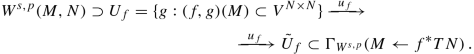
  These charts cover W ^{s, p}(M, N), by the following argument: Since C ^∞(M, N) is dense in W ^{s, p}(M, N) and since W ^{s, p}(M, N) ⊂ C ^k(M, N) via a continuous injection for $0\le k<s-\dim (M)/p$, a suitable -norm neighborhood of g ∈ W ^{s, p}(M, N) contains a smooth f ∈ C ^∞(M, N), thus f ∈ U _g and by symmetry of V ^N×N we have g ∈ U _f. This is true for compact M. For a compact Whitney manifold germ we can apply this argument in a compact neighborhood which is a manifold with smooth boundary L of M in $\tilde M$ and apply the argument there.

In each case, we equip C ^∞(M, N) or C ^k(M, N) or W ^{s, p}(M, N) with the initial topology with respect to all chart mappings described above: The coarsest topology, so that all chart mappings u _f are continuous.

For non-compact M the direct limit over a compact exhaustion L of M in the category of locally convex vector spaces is strictly coarser that the direct limit in the category of Hausdorff topological spaces. It is more convenient to use the latter topology which is called c ^∞ topology; compare with Sect. 2.1.

5.4 Lemma

• (1) If M is a compact smooth manifold or is a compact Whitney manifold germ,

  

  For smooth f ∈ C ^∞(M, N),

  

• (2) If M is a non-compact smooth manifold of Whitney manifold germ, the sections on the right-hand side have to satisfy the corresponding conditions of Lemma 5.1(4).

For a compact Whitney manifold germ M the space is a direct summand in the space of sections with support in $\mathbb R\times L$ for a fixed compact set $L\subset \tilde M$ containing M in its interior. Likewise is a direct summand in the space of -sections. One could introduce similar notation for .

Proof

This follows from Lemma 5.1. □

5.5 Lemma

Let M be a smooth manifold or Whitney manifold germ, compact or not, and let N be a manifold. Then the chart changes for charts centered on smooth mappings are smooth (C ^∞) on the space C ^∞(M, N), also on C ^k(M, N) for $k\in \mathbb N_{\ge 0}$, and on W ^{s, p}(M, N) for 1 < p < ∞ and $s>\dim (M)/p$:

$$\displaystyle \begin{aligned}\tilde U_{f_1}\ni s \mapsto (u_{f_2,f_1})_*(s) := (\exp^{\bar g}_{f_2})^{-1}\operatorname{\circ} \exp^{\bar g}_{f_1}\operatorname{\circ} s\in \tilde U_{f_2}\,. \end{aligned}$$

Proof

This follows from Lemma 5.2, since any chart change is just compositions from the left by a smooth fiber respecting locally defined diffeomorphism. □

5.6 Lemma

• (1) If M is a compact manifold or a compact Whitney manifold germ, then

  $$\displaystyle \begin{aligned}C^\infty(\mathbb R,C^\infty(M,N))\cong C^\infty(\mathbb R\times M,N)\,.\end{aligned}$$

• (2) If M is not compact, $C^\infty (\mathbb R,C^\infty (M,N))$ consists of all smooth $c:\mathbb R\times M\to N$ such that

  • for each compact interval $[a,b]\subset \mathbb R$ there is a compact subset K ⊂ M such that c(t, x) is constant in t ∈ [a, b] for each x ∈ M ∖ K.

Proof

By Lemma 5.4. □

5.7 Lemma

Composition $(f,g)\mapsto g\operatorname {\circ } f$ is smooth as a mapping

$$\displaystyle \begin{gathered} C^\infty(P,M)\times C^\infty(M,N)\to C^\infty(P,N) \\ C^k(P,M)\times C^\infty(M,N)\to C^k(P,N) \\ W^{s,p}(P,M)\times C^\infty(M,N)\to W^{s,p}(P,N) \end{gathered} $$

for P a manifold or a Whitney manifold germ, compact or not, and for M and N manifolds.

For more general M the description becomes more complicated. See the special case of the diffeomorphism group of a Whitney manifold germ M in Sect. 6.3 below.

Proof

Since it maps smooth curves to smooth curves. □

5.8 corollary

For M a manifold or a Whitney manifold germ and a manifold N, the tangent bundle of the manifold C ^∞(M, N) of mappings is given by

Proof

This follows from the chart structure and the fact that sections of f ^∗ TN → M correspond to mappings s : M → TN with $\pi _N\operatorname {\circ } s =f$. □

5.9 Sprays Respecting Fibers of Submersions

Sprays are versions of Christoffel symbols and lead to exponential mappings. They are easier to adapt to fibered manifolds than Riemannian metrics. Recall that a spray S on a manifold N without boundary is a smooth mapping S : TN → T ² N with the following properties:

• $\pi _{TN}\operatorname {\circ } S= \operatorname {Id}_{TN}$; S is a vector field.

• $T(\pi _N)\operatorname {\circ } S= \operatorname {Id}_{TN}$; S is a “differential equation of second order.”

• Let $m^N_t:TN\to TN$ and $m^{TN}_t:T^2N\to T^2N$ be the scalar multiplications. Then $S\operatorname {\circ } m^N_t = T(m^N_t).m^{TN}_t.S$.

Locally, in charts of TN and T ² N induced by a chart of N, a spray looks like S(x, v) = (x, v;v; Γ(x, v)) where Γ is quadratic in v. For a spray $S\in \mathfrak X(TN)$ on a manifold N, we let $\exp (X):=\pi _N(\operatorname {Fl}^S_1(X))$, then the mapping is smooth, defined on an open neighborhood V of the zero section in TN, which is called the exponential mapping of the spray S. Since $T_{0_x}(\exp |{ }_{T_xN})=\operatorname {Id}_{T_xN}$ (via $T_{0_x}(T_xN)=T_xN$), by the inverse function theorem $\exp _x:=\exp |{ }_{T_xN}$ is a diffeomorphism near 0_x in TN onto an open neighborhood of x in N. Moreover the mapping is a diffeomorphism from an open neighborhood $\tilde V$ of the zero section in TN onto an open neighborhood of the diagonal in N × N.

Lemma

Let q : N → M be a smooth surjective submersion between connected manifolds without boundary. Then there exists a spray S on N which is tangential to the fibers of q, i.e., S(T(q ⁻¹(x))) ⊂ T ²(q ⁻¹(x)) for each x ∈ M.

This is a simplified version of [69, 10.9].

Proof

In suitable charts on N and M the submersion q looks like a linear projection (y ₁, y ₂)↦y ₁. The local expression T(chart) → T ²(chart) of a spray is

$$\displaystyle \begin{aligned} &S\big((y_1,y_2),(v_1,v_2)\big) = \\&\qquad \quad = \big((y_1,y_2),(v_1,v_2);(v_1,v_2),(\Gamma^1(y_1,y_2;v_1,v_2),\Gamma^2(y_1,y_2,v_1,v_2))\big), \end{aligned} $$

where Γⁱ(y ₁, y ₂, v ₁, v ₂) is quadratic in (v ₁, v ₂). The spray is tangential to the fibers of q if and only if Γ¹(y ₁, y ₂, 0, v ₂) = 0. This clearly exists locally (e.g., choose Γ¹ = 0). Now we use a partition of unity (φ _α) subordinated to a cover N =⋃_α U _α with such charts and glue local sprays with the induced partition of unity $(\varphi _\alpha \operatorname {\circ } \pi _N)$ subordinated to the cover TN =⋃_α TUα for the vector bundle π _TN : T ² N → TN. Locally this looks like (where y = (y ₁, y ₂), etc.)

$$\displaystyle \begin{aligned} \Big(\sum_\alpha (\varphi_\alpha\operatorname{\circ} \pi_N).S_\alpha\Big)(y,v) &= \Big(y,v; \sum_\alpha \varphi_\alpha(y)v, \sum_\alpha \varphi_\alpha(y)\big(\Gamma^1_\alpha(y,v),(\Gamma^2_\alpha(y,v)\big) \Big) \\& = \Big(y,v; v, \big(\sum_\alpha \varphi_\alpha(y)\Gamma^1_\alpha(y,v),\sum_\alpha \varphi_\alpha(y)\Gamma^2_\alpha(y,v)\big) \Big) \end{aligned} $$

and is therefore a spray which is tangential to the fibers of q. □

5.10 Proposition

([69, 10.10]) Let q : N → M be a smooth surjective submersion between connected manifolds without boundary. The space S ^q(M, N) of all smooth sections of q is a splitting smooth submanifold of C ^∞(M, N). Similarly, the spaces $S^q_{C^N}(M,N)$ and $S^q_{W^{s,p}}(M,N)$ of C ^N-sections and W ^{s, p}-sections are smooth splitting submanifolds of C ^N(M, N) or W ^{s, p}(M, N) (for $s>\dim (M)/p$), respectively.

The proof given here is simpler than the one in [69, 10.10].

Proof

Let us first assume that M is compact. Given a smooth section f ∈ S ^q(M, N), consider the chart centered at f from Sect. 5.3

where we use the exponential mapping with respect to a spray S on N which is tangential to the fibers of q. Using an unrelated auxiliary Riemannian metric $\bar g$ on N we can smoothly split the tangent bundle TN = V ^q(N) ⊕ H ^q(N) into the vertical bundle of all vectors tangent to the fibers of q, and into its orthogonal complement with respect to $\bar g$. The orthonormal projections $P^{\bar g}:TN \to V^q(N)$ and $\operatorname {Id}_{TN}-P^{\bar g}: TN\to H^q(N)$ induce the direct sum decomposition

$$\displaystyle \begin{aligned}\Gamma(M\gets f^*TN) = \Gamma(M\gets f^*V^q(N))\oplus \Gamma(M\gets f^*TN) \quad s\mapsto (P^{\bar g}.s, s-P^{\bar g}.s). \end{aligned}$$

Now g ∈ U _f is in S ^q(M, N) if and only if u _f(g) ∈ Γ(f ^∗ V ^q(N)).

If M is not compact we may use the spaces of sections with compact support as described in Sect. 5.3. Similarly for the cases of C ^N-sections or W ^{s, p}-sections. □

5.11 Corollary

Let p : E → M be a fiber bundle over a compact Whitney manifold germ M. Then the space Γ(E) of smooth sections is a splitting smooth submanifold of C ^∞(M, E). Likewise for the spaces $\Gamma _{C^n}(E)$ and $\Gamma _{W^{s,p}}(E)$ of C ^N-sections and W ^{s, p}-sections.

Proof

Recall from Sect. 4.8 that $E=\tilde E|{ }_M$ for a smooth fiber bundle $\tilde E\to \tilde M$. There the result follows from 5.10. Using (fixed) extension operators

$$\displaystyle \begin{aligned}\Gamma(M\gets f^*TE)\to \Gamma_L(\tilde M\gets \tilde f^*T\tilde E), \end{aligned}$$

etc. we can extend this the case of Whitney manifold germs. □

6 Regular Lie Groups

6.1 Regular Lie Groups

We consider a smooth Lie group G with Lie algebra $\mathfrak g=T_eG$ modeled on convenient vector spaces. The notion of a regular Lie group is originally due to [86,87,88,89,90,91] for Fréchet Lie groups, was weakened and made more transparent by Milnor [78], and then carried over to convenient Lie groups in [56], see also [55, 38.4]. We shall write μ : G × G → G for the multiplication with x.y = μ(x, y) = μ _x(y) = μ ^y(x) for left and right translation.

A Lie group G is called regular if the following holds:

• For each smooth curve $X\in C^{\infty }(\mathbb R,\mathfrak g)$ there exists a curve $g\in C^{\infty }(\mathbb R,G)$ whose right logarithmic derivative is X, i.e.,

  $$\displaystyle \begin{aligned}\begin{cases} g(0) &= e \\ \partial_t g(t) &= T_e(\mu^{g(t)})X(t) = X(t).g(t). \end{cases} \end{aligned}$$

  The curve g is uniquely determined by its initial value g(0), if it exists.

• Put $\operatorname {evol}^r_G(X)=g(1)$ where g is the unique solution required above. Then $\operatorname {evol}^r_G: C^{\infty }(\mathbb R,\mathfrak g)\to G$ is required to be C ^∞ also. We have $\operatorname {Evol}^X_t:= g(t) =\operatorname {evol}^r_G(tX)$.

Of course we could equivalently use the left logarithmic derivative and the corresponding left evolution operator. Group inversion maps the two concepts into each other. See [55, Section 38] for more information. Up to now, every Lie group modeled on convenient vector spaces is regular.

There are other notions of regularity for infinite dimensional Lie groups: For example, one may require that each curve $X\in L^1_{\text{loc}}(\mathbb R,\mathfrak g)$ admits an absolutely continuous curve $\operatorname {Evol}^X:\mathbb R\to G$ whose right logarithmic derivative is X. See [46] or [49] and references therein. It might be that all these notions of regularity are equivalent for Lie groups modeled on convenient vector spaces.

6.2 Theorem

For each manifold M with or without corners, the diffeomorphism group $\operatorname {Diff}(M)$ is a regular Lie group. Its Lie algebra is the space $\mathfrak X(M)$ of all vector fields with the negative of the usual bracket as Lie bracket, if M is compact without boundary. It is the space $\mathfrak X_c(M)$ of fields with compact support, if M is an open manifold. It is the space $\mathfrak X_\partial (M)$ of Sect. 4.7 of vector fields tangent to the boundary, if M is a compact manifold with corners. If M is not compact with corners, then the Lie algebra is the space $\mathfrak X_{c,\partial }(M)$ of boundary respecting vector fields with compact support.

Proof

If M is a manifold without boundary then . If M is open, then the group of diffeomorphisms differing from the identity only on a compact set is open in $\operatorname {Diff}(M)$.

If M has corners we use an open manifold $\tilde M$ containing M as a submanifold with corners as in Lemma 3.2. In the description of the chart structure in Sect. 5.3 for $\operatorname {Diff}(\tilde M)$ we have to use the exponential mapping for a geodesic spray on $\tilde M$ such that each component of each ∂ ^q M is totally geodesic. This spray exists; see Sect. 3.7 or Sect. 5.9. Restricting all sections to M then yields a smooth chart centered at the identity for $\operatorname {Diff}(M)$. Then we use right translations of this chart. The explicit chart structure on $\operatorname {Diff}(M)$ is described in [69, 10.16]. Extending all sections to $\tilde M$ via a fixed continuous linear Whitney extension operator respecting compact support identifies $\operatorname {Diff}(M)$ as a splitting smooth closed submanifold of $\operatorname {Diff}(\tilde M)$, but not as a subgroup.

Composition is smooth by restricting it from C ^∞(M, M) × C ^∞(M, M), using Lemma 5.7 and its extension to the situation with corners.

Inversion is smooth: If t↦f(t, ) is a smooth curve in $\operatorname {Diff}(M)$, then f(t, )⁻¹ satisfies the implicit equation f(t, f(t, )⁻¹(x)) = x, so by the finite dimensional implicit function theorem, (t, x)↦f(t, )⁻¹(x) is smooth. So inversion maps smooth curves to smooth curves, and is smooth.

Let X(t, x) be a time-dependent vector field on M (in $C^\infty (\mathbb R,\mathfrak X(M))$). Then $\operatorname {Fl}^{\partial _t\times X}_s(t,x)=(t+s,\operatorname {Evol}^X(t,x))$ satisfies the ordinary differential equation

$$\displaystyle \begin{aligned}\quad \partial_t\operatorname{Evol}(t,x) = X(t,\operatorname{Evol}(t,x)). \end{aligned}$$

If $X(s,t,x)\in C^\infty (\mathbb R^2,\mathfrak X(M))$ is a smooth curve of smooth curves in $\mathfrak X(M)$, then obviously the solution of the equation depends smoothly also on the further variable s, thus $\operatorname {evol}$ maps smooth curves of time dependent vector fields to smooth curves of diffeomorphism. □

6.3 The Diffeomorphism Group of a Whitney Manifold Germ

For a Whitney manifold germ , we consider the diffeomorphism group

$$\displaystyle \begin{aligned} \operatorname{Diff}(M)=\{\varphi|{}_M: \varphi&\in C^{\infty}(\tilde M,\tilde M),\; \varphi(M)=M, \\ &\varphi \text{ is a diffeomorphism on an open neighborhood of }M\}\,. \end{aligned} $$

We also consider the following set $\mathcal C$ of smooth curves: Those $c:\mathbb R\to \operatorname {Diff}(M)$ which are of the form $c=\tilde c|{ }_{\mathbb R\times M}$ for a smooth

$$\displaystyle \begin{aligned}\tilde c:\mathbb R\times \tilde M\to \tilde M\quad \text{ with } \tilde c(t,)|{}_M\in \operatorname{Diff}(M) \text{ for each }t\in \mathbb R. \end{aligned}$$

Note that for t in a compact interval $\tilde c(t,)$ is a diffeomorphism on a fixed open neighborhood of M in $\tilde M$.

6.4 Theorem

For a Whitney manifold germ M the group $\operatorname {Diff}(M)$ is a Frölicher space and a group with smooth composition and inversion. It has a convenient Lie algebra $\mathfrak X_{c,\partial }(M)$ with the negative of the usual bracket as Lie bracket, and it is regular: There exists an evolution operator and it is smooth.

Proof

The Frölicher space structure is the one induced by the set $\mathcal C$ of smooth curves described above. I do not know whether this set of smooth curves is saturated, i.e., $\mathcal C= \mathcal C_{\operatorname {Diff}(M)}$ in the notation of Sect. 2.7; this might depend on the structure of the boundary.

The proof is now quite similar to the one of Sect. 6.1. We claim that composition maps $\mathcal C\times \mathcal C$ to $\mathcal C\subseteq \mathcal C_{\operatorname {Diff}(M)}$, and that inversion maps $\mathcal C$ to $\mathcal C\subseteq \mathcal C_{\operatorname {Diff}(M)}$. Since by definition each curve $c\in \mathcal C$ extend to a smooth mapping $\tilde c:\mathbb R\times \tilde M\to \tilde M$ we can actually use a slight adaption of the proof of Sect. 6.1 for open manifolds. □

6.5 The Connected Component of $\operatorname {Diff}(M)$ for a Whitney Manifold Germ M

We consider a Whitney manifold germ $M\subset \tilde M$. As usual for Frölicher space, we equip $\operatorname {Diff}(M)$ with the final topology with respect to all smooth curves in in the generating set $\mathcal C$ as described in Sect. 6.3. $\operatorname {Diff}(M)$ is actually a topological group, with the refined topology (i.e., the c ^∞-topology) on $\operatorname {Diff}(M)\times \operatorname {Diff}(M)$. Let $\operatorname {Diff}_0(M)$ be the connected component of the identity in $\operatorname {Diff}(M)$ with respect to this topology.

Theorem

For a Whitney manifold germ $M\subset \tilde M$ we actually have

$$\displaystyle \begin{aligned}\operatorname{Diff}_0(M) = \{\tilde\varphi|{}_M: \tilde\varphi\in \operatorname{Diff}_0(\tilde M),\; \tilde\varphi(M) = M\}\,. \end{aligned}$$

Consequently, the subgroup

$$\displaystyle \begin{aligned}\operatorname{Diff}{\tilde{\,}}(M) = \{\tilde\varphi|{}_M: \tilde \varphi\in \operatorname{Diff}(\tilde M), \, \tilde\varphi(M)=M\}\end{aligned}$$

is an open subgroup in $\operatorname {Diff}(M)$ and thus a normal subgroup, and the corresponding generating set $\mathcal C$ of smooth curves in $\operatorname {Diff}{\tilde {\,}}(M)$ is saturated.

Proof

Let $\varphi \in \operatorname {Diff}_0(M)$. Then there exists a smooth curve $\varphi :\mathbb R\to \operatorname {Diff}(M)$ with $\varphi (0)=\operatorname {Id}$ and φ(1) = φ of the form $\varphi =\tilde c|{ }_{\mathbb R\times M}$ where $\tilde c:\mathbb R\times \tilde M\to \tilde M$ is a smooth mapping with $\tilde c(t,)|{ }_M\in \operatorname {Diff}(M)$ for each $t\in \mathbb R$. Then X(t, x) = (∂ _t φ(t))(φ(t)⁻¹(x)) gives us a time-dependent vector field which is defined on [0, 1] × U for some open neighborhood U of M in $\tilde M$, by the definition of $\operatorname {Diff}(M)$ in Sect. 6.3. Using a continuous extension operator on X|_[0,1]×M and a smooth bump function gives us a smooth time-dependent vector field $\tilde X:[0,1]\times \tilde M\to T\tilde M$ with support in a fixed open neighborhood, say, such that $\tilde X|{ }_{[0,1]\times M}= X|{ }_{[0,1]\times M}$. Solving the ODE $\partial _t \tilde \varphi (t.x) = \tilde X(t,\tilde \varphi (t,x))$ on $\tilde M$ gives us for t = 1 a diffeomorphism $\tilde \varphi \in \operatorname {Diff}(\tilde M)$ which extends φ.

Given any $\varphi \in \operatorname {Diff}{\tilde {\,}}(M)$, the coset $\varphi .\operatorname {Diff}_0(M)\subset \operatorname {Diff}(M)$ is the connected component of φ in $\operatorname {Diff}(M)$. This shows that $\operatorname {Diff}{\tilde {\,}}(M)$ is open in $\operatorname {Diff}(M)$. □

The construction in the proof above actually describes a smooth mapping

$$\displaystyle \begin{aligned}\mathcal E:\{c\in C^\infty(\mathbb R, \operatorname{Diff}_0(M)):c(0)=\operatorname{Id}\}\to\{\tilde\varphi\in \operatorname{Diff}_0(\tilde M): \tilde\varphi(M)=M\}\end{aligned}$$

such that $\mathcal E(c)|{ }_M = c(1)$, since another smooth real parameter s goes smoothly through solving the ODE.

6.6 Remark

In this paper I refrain from trying to give a general definition of a regular Frölicher group, which would be an abstract concept that catches the essential properties of $\operatorname {Diff}(M)$ for a Whitney manifold germ $M\subset \tilde M$. Let me just remark, that it probably would fit into the concept of manifolds based on smooth curves instead of charts as developed in [72]; those among them whose tangent spaces are Banach spaces turn out to be Banach manifolds. Some Lie theoretic tools are developed in the beginning of Sect. 8.5 below.

6.7 Regular (Right) Half Lie Groups

A smooth manifold G modeled on convenient vector spaces is called a (right) half Lie group, if it is a group such that multiplication μ : G × G → G and inversion ν : G → G are continuous (note that here we have to take the induced c ^∞-topology on the product G × G if the model spaces are not Fréchet), but each right translation μ ^x : G → G, μ ^x(y) = y.x is smooth. The notion of a half Lie group was coined in [60]. See [64] for a study of half Lie groups in general, concentrating on semidirect products with representation spaces.

Not every tangent vector in T _e G can be extended to a left invariant vector field on the whole group, but they can be extended to right invariant vector fields, which are only continuous and not differentiable in general. The same holds for right invariant Riemannian metrics. The tangent space at the identity is not a Lie algebra in general; thus we refrain from calling it $\mathfrak g$. Have a look at the examples in Theorem 6.8 to get a feeling for this.

Let us discuss regularity on a (right) half Lie group G: For a smooth curve $g:\mathbb R\to G$ the velocity curve $g':\mathbb R \to TG$ is still smooth, and for fixed t the right logarithmic derivative $X(t):=g'(t).g(t)^{-1}=T(\mu ^{g(t)^{-1}}).g'(t)$ lies in T _e G, but t↦X(t) is only continuous $\mathbb R\to T_{e}G$. A (right) half Lie group G is called C ⁰ -regular if for every C ⁰-curve $X:\mathbb R\to T_{e}G$ there exists a C ¹-curve $\operatorname {Evol}^X=g:\mathbb R\to G$ with g(0) = e and g′(t) = X(t).g(t) = T(μ ^g(t)).X(t). We also require that $X\mapsto \operatorname {Evol}^X$ is smooth $C^0(\mathbb R,T_eG)\to C^1(\mathbb R, G)$.

6.8 Theorem

[Diffeomorphism Groups of Finite Degrees of Differentiability]

• (1) For a compact smooth manifold M, possibly with corners, and for any $n\in \mathbb N_{\ge 1}$ the group $\operatorname {Diff}_{C^n}(M)$ of C ⁿ-diffeomorphism of M is a C ⁰-regular half Lie group.

• (2) For a compact smooth manifold M, possibly with corners, and for any $s\ge \dim {M}/p +1$, the group $\operatorname {Diff}_{W^{s,p}}(M)$ of Sobolev W ^{s, p}-diffeomorphism of M is a C ⁰-regular half Lie group.

Note that the group of homeomorphisms of M is not open in $C^0_{\text{nice}}(M,M)$; see the proof below for $C^{\infty }_{\text{nice}}$. Also note that $T_{\operatorname {Id}}\operatorname {Diff}_{C^n}(M) = \mathfrak X_{\partial , C^n}(M)$ is the space of C ⁿ-vector fields which are tangent to the boundary. This is not a Lie algebra, since the Lie bracket of two C ⁿ fields is a C ⁿ⁻¹ field in general.

Proof

• (1) Following [69, 10.16], we construct the smooth manifold structure by using the exponential mapping of a spray on M which is tangential to the boundary; for existence see Sects. 3.7 and 5.9. Let $C^{n}_{\text{nice}}(M,M,)$ be the set of all C ⁿ-mappings f : M → M with f ⁻¹(∂ ^q M) = ∂ ^q M for each q. Then we use the (restriction of the) chart structure described in Sect. 5.3, using this exponential mappings, and using only charts centered at smooth mappings $f\in C^{\infty }_{\text{nice}}(M,M)$, as follows:

  

  By the symmetry of V ^M×M (see Sect. 5.3) these charts cover $C^{n}_{\text{nice}}(M,M)$, and the chart changes are smooth since they map smooth curves (as described in Lemma 5.1(2)) to smooth curves; compare to Lemma 5.7. The group $\operatorname {Diff}_{C^n}(M)$ is open in $C^{n}_{\text{nice}}(M,M)$, by the implicit function theorem and some easy arguments.

  Continuity of composition and inversion are easy to check. Right translations are smooth since they map smooth curves.

  C ¹-regularity follows easily: Given $X\in C^0(\mathbb R,T_{\operatorname {Id}}\operatorname {Diff}_{C^n}(M))$, view it as a time-dependent C ⁿ-vector field on M which is tangential to the boundary, a continuous curve in $\mathfrak X_\partial (M)$ and solve the corresponding ODE. The evolution operator $\operatorname {Evol}$ is smooth, since it maps smooth curves to smooth curves by standard ODE-arguments.

• (2) This follows easily by adapting the proof of (1) above, using that $\operatorname {Diff}_{W^{s,p}}M\subset \operatorname {Diff}_{C^1}(M)$ by the Sobolev embedding lemma.

□

6.9 Groups of Smooth Diffeomorphisms on $\mathbb R^n$

If we consider the group of all orientation preserving diffeomorphisms $\operatorname {Diff}(\mathbb R^n)$ of $\mathbb R^n$, it is not an open subset of $C^\infty (\mathbb R^n,\mathbb R^n)$ with the compact C ^∞-topology. So it is not a smooth manifold in the usual sense, but we may consider it as a Lie group in the cartesian closed category of Frölicher spaces, see [55, Section 23], with the structure induced by the injection $f\mapsto (f,f^{-1})\in C^\infty (\mathbb R^n,\mathbb R^n)\times C^\infty (\mathbb R^n,\mathbb R^n)$. Or one can use the setting of “manifolds” based on smooth curves instead of charts, with lots of extra structure (tangent bundle, parallel transport, geodesic structure), described in [72]; this gives a category of smooth “manifolds” where those which have Banach spaces as tangent fibers are exactly the usual smooth manifolds modeled on Banach spaces, which is cartesian closed: C ^∞(M, N) and $\operatorname {Diff}(M)$ are always “manifolds” for “manifolds” M and N, and the exponential law holds.

We shall now describe regular Lie groups in $\operatorname {Diff}(\mathbb R^n)$ which are given by diffeomorphisms of the form $f = \operatorname {Id}_{\mathbb R} + g$ where g is in some specific convenient vector space of bounded functions in $C^\infty (\mathbb R^n,\mathbb R^n)$. Now we discuss these spaces on $\mathbb R^n$, we describe the smooth curves in them, and we describe the corresponding groups. These results are from [77] and from [60, 61] for the more exotic groups.

The Group $\operatorname {Diff}_{\mathcal B}(\mathbb R^n)$

The space $\mathcal B(\mathbb R^n)$ (called $\mathcal D_{L^\infty }(\mathbb R^n)$ by Schwartz [96]) consists of all smooth functions which have all derivatives (separately) bounded. It is a Fréchet space. By Vogt [105], the space $\mathcal B(\mathbb R^n)$ is linearly isomorphic to $\ell ^\infty \hat \otimes \, \mathfrak s$ for any completed tensor-product between the projective one and the injective one, where $\mathfrak s$ is the nuclear Fréchet space of rapidly decreasing real sequences. Thus $\mathcal B(\mathbb R^n)$ is not reflexive, not nuclear, not smoothly paracompact.

The space $C^\infty (\mathbb R,\mathcal {B}(\mathbb R^n))$ of smooth curves in $\mathcal {B}(\mathbb R^n)$ consists of all functions $c\in C^\infty (\mathbb R^{n+1},\mathbb R)$ satisfying the following property:

• For all $k\in \mathbb N_{\ge 0}$ , $\alpha \in \mathbb N_{\ge 0}^n$ and each $t\in \mathbb R$ the expression $\partial _t^{k}\partial ^\alpha _x c(t,x)$ is uniformly bounded in $x\in \mathbb R^n$ , locally in t.

To see this use Theorem 2.6 for the set $\{\operatorname {ev}_x: x\in \mathbb R\}$ of point evaluations in $\mathcal {B}(\mathbb R^n)$. Here $\partial ^\alpha _x = \frac {\partial ^{|\alpha |}}{\partial x^\alpha }$ and $c^k(t)=\partial _t^kf(t,\quad )$.

$\operatorname {Diff}^+_{\mathcal B}(\mathbb R^n)=\bigl \{f=\operatorname {Id}+g: g\in \mathcal B(\mathbb R^n)^n, \det (\mathbb I_n + dg)\ge \varepsilon > 0 \bigr \}$ denotes the corresponding group, see below.

The Group $\operatorname {Diff}_{W^{\infty ,p}}(\mathbb R^n)$

For 1 ≤ p < ∞, the space

$$\displaystyle \begin{aligned}W^{\infty,p}(\mathbb R^n)=\bigcap_{k\ge 1}L^p_k(\mathbb R^n)\end{aligned}$$

is the intersection of all L ^p-Sobolev spaces, the space of all smooth functions such that each partial derivative is in L ^p. It is a reflexive Fréchet space. It is called $\mathcal D_{L^p}(\mathbb R^n)$ in [96]. By Vogt [105], the space $W^{\infty ,p}(\mathbb R^n)$ is linearly isomorphic to $\ell ^p\hat \otimes \, \mathfrak s$. Thus it is not nuclear, not Schwartz, not Montel, and smoothly paracompact only if p is an even integer.

The space $C^\infty (\mathbb R,H^\infty (\mathbb R^n))$ of smooth curves in $W^{\infty ,p}(\mathbb R^n)$ consists of all functions $c\in C^\infty (\mathbb R^{n+1},\mathbb R)$ satisfying the following property:

• For all $k\in \mathbb N_{\ge 0}$ , $\alpha \in \mathbb N_{\ge 0}^n$ the expression $\|\partial _t^{k}\partial ^\alpha _xf(t,\quad )\|{ }_{L^p(\mathbb R^n)}$ is locally bounded near each $t\in \mathbb R$.

The proof is literally the same as for $\mathcal B(\mathbb R^n)$, noting that the point evaluations are continuous on each Sobolev space $L^p_k$ with $k>\frac np$.

$\operatorname {Diff}^+_{W^{\infty ,p}}(\mathbb R^n)=\bigl \{f=\operatorname {Id}+g: g\in W^{\infty ,p}(\mathbb R^n)^n, \det (\mathbb I_n + dg)>0\bigr \}$ denotes the corresponding group.

The Group $\operatorname {Diff}_{\mathcal S}(\mathbb R^n)$

The algebra $\mathcal S(R^n)$ of rapidly decreasing functions is a reflexive nuclear Fréchet space.

The space $C^\infty (\mathbb R,\mathcal S(\mathbb R^n))$ of smooth curves in $\mathcal S(\mathbb R^n)$ consists of all functions $c\in C^\infty (\mathbb R^{n+1},\mathbb R)$ satisfying the following property:

• For all $k,m\in \mathbb N_{\ge 0}$ and $\alpha \in \mathbb N_{\ge 0}^n$ , the expression $(1+|x|{ }^2)^m\partial _t^{k}\partial ^\alpha _xc(t,x)$ is uniformly bounded in $x\in \mathbb R^n$ , locally uniformly bounded in $t\in \mathbb R$.

$\operatorname {Diff}^+_{\mathcal S}(\mathbb R^n)=\bigl \{f=\operatorname {Id}+g: g\in \mathcal S(\mathbb R^n)^n, \det (\mathbb I_n + dg)>0\bigr \}$ is the corresponding group.

The Group $\operatorname {Diff}_{c}(\mathbb R^n)$

The algebra $C^\infty _c(\mathbb R^n)$ of all smooth functions with compact support is a nuclear (LF)-space.

The space $C^\infty (\mathbb R,C^\infty _c(\mathbb R^n))$ of smooth curves in $C^\infty _c(\mathbb R^n)$ consists of all functions $f\in C^\infty (\mathbb R^{n+1},\mathbb R)$ satisfying the following property:

• For each compact interval [a, b] in $\mathbb R$ there exists a compact subset $K\subset \mathbb R^n$ such that f(t, x) = 0 for $(t,x)\in [a,b]\times (\mathbb R^n\setminus K)$.

$\operatorname {Diff}_c(\mathbb R^n)=\bigl \{f=\operatorname {Id}+g: g\in C^\infty _c(\mathbb R^n)^n, \det (\mathbb I_n + dg)>0\bigr \}$ is the corresponding group. The case $\operatorname {Diff}_c(\mathbb R^n)$ is well-known since 1980.

Ideal Properties of Function Spaces

The function spaces discussed are boundedly mapped into each other as follows:

and each space is a bounded locally convex algebra and a bounded $\mathcal B(\mathbb R^n)$-module. Thus each space is an ideal in each larger space.

6.10 Theorem

([77] and [60]) The sets of diffeomorphisms

$$\displaystyle \begin{aligned}\operatorname{Diff}_c(\mathbb R^n),\quad \operatorname{Diff}_{\mathcal S}(\mathbb R^n),\quad \operatorname{Diff}_{H^\infty}(\mathbb R^n), \text{ and } \operatorname{Diff}_{\mathcal B}(\mathbb R^n)\end{aligned}$$

are all smooth regular Lie groups. We have the following smooth injective group homomorphisms:

Each group is a normal subgroup in any other in which it is contained, in particular in $\operatorname {Diff}_{\mathcal B}(\mathbb R^n)$.

The proof of this theorem relies on repeated use of the Faà di Bruno formula for higher derivatives of composed functions. This offers difficulties on non-compact manifolds, where one would need a non-commutative Faà di Bruno formula for iterated covariant derivatives. In the paper [60] many more similar groups are discussed, modeled on spaces of Denjoy–Carleman ultradifferentiable functions. It is also shown that for p > 1 the group $\operatorname {Diff}_{W^{\infty ,p}\cap L^1}(\mathbb R^n)$ is only a topological group with smooth right translations—a property which is similar to the one of finite order Sobolev groups $\operatorname {Diff}_{W^{k,p}}(\mathbb R^n)$. Some of these groups were used extensively in [80].

6.11 Corollary

$\operatorname {Diff}_{\mathcal B}(\mathbb R^n)$ acts on Γ_c, $\Gamma _{\mathcal S}$ and $\Gamma _{H^\infty }$ of any tensor bundle over $\mathbb R^n$ by pullback. The infinitesimal action of the Lie algebra $\mathfrak X_{\mathcal B}(\mathbb R^n)$ on these spaces by the Lie derivative maps each of these spaces into itself. A fortiori, $\operatorname {Diff}_{H^\infty }(\mathbb R^n)$ acts on $\Gamma _{\mathcal S}$ of any tensor bundle by pullback.

6.12 Trouvé Groups

For the following see [85, 103, 108]. Trouvé groups are useful for introducing topological metrics on certain groups of diffeomorphism on $\mathbb R^d$ starting from a suitable reproducing kernel Hilbert space of vector fields without using any Lie algebra structure; see Sect. 8.12 below.

Consider a time-dependent vector field $X:[0,1] \times \mathbb R^d\to \mathbb R$ of sufficient regularity (e.g., continuous in t ∈ [0, 1] and Lipschitz continuous in $x\in \mathbb R^d$ with t-integrable global Lipschitz constant) so that

$$\displaystyle \begin{aligned}x(t) = x_0 + \int_0^t X(s,x(s))\,ds\end{aligned} $$

is uniquely solvable for all t ∈ [0, 1] and $x_0\in \mathbb R^d$. Then we consider the evolution $\operatorname {evol}^X(x_0) = x(1)$. For $X\in L^1([0,1], C^1_b(\mathbb R^d,\mathbb R)^d)$ (where $f\in C^k_b$ if all iterated partial derivatives of order between 0 and k are continuous and globally bounded) we have $\operatorname {evol}^X\in \operatorname {Id} + C^1_b(\mathbb R^d, \mathbb R^d)$ and is a diffeomorphism with $(\operatorname {evol})^{-1} \in \operatorname {Id} + C^1_b(\mathbb R^d, \mathbb R^d)$. Given a convenient locally convex vector space $\mathcal A(\mathbb R^d,\mathbb R^d)$ of mappings $\mathbb R^d\to \mathbb R^d$ which continuously embeds into $C^1_b(\mathbb R^d,\mathbb R^d)$ and a suitable family of mappings $[0,1]\to \mathcal A(\mathbb R^d,\mathbb R^d)$, the associated Trouvé group is given by

$$\displaystyle \begin{aligned}\mathcal G_{\mathcal A} := \{\operatorname{evol}^X: X\in \mathcal F_ {\mathcal A}\},\end{aligned} $$

where $\mathcal F_ {\mathcal A} = \mathcal F([0,1], \mathcal A(\mathbb R^d,\mathbb R^d))$ is a suitable vector space of time-dependent vector fields. It seems that for a wide class of spaces $\mathcal A$ the Trouvé group $\mathcal G_{\mathcal A}$ is independent of the choice of $\mathcal F_{\mathcal A}$ if the latter contains the piecewise smooth curves and is contained in the curves which are integrable by seminorms; a precise statement is still lacking, but see [82, 84, 85], and citations therein. The space $\mathcal A$ is called $\mathcal F_ {\mathcal A}$ -ODE-closed if $\operatorname {evol}^X \in \operatorname {Id}+\mathcal A(\mathbb R^d,\mathbb R^d)$ for each $X\in \mathcal F_ {\mathcal A}$. For ODE-closed $\mathcal A$ the Trouvé group $\mathcal G_{\mathcal A}$ is contained in $\operatorname {Id}+ \mathcal A(\mathbb R^d,\mathbb R^d)$.

For some spaces $\mathcal A$ it has been proved that $\mathcal F_{\mathcal A}$ is equal to the connected component of the identity of

$$\displaystyle \begin{aligned}\{\operatorname{Id} + f: f\in \mathcal A(\mathbb R^d,\mathbb R^d), \inf_{x\in \mathbb R^d} \det df(x) > -1\},\end{aligned} $$

namely

• For Sobolev spaces W ^{k, 2} with k > d∕2 by Bruveris and Vialard [22]; $\mathcal G_{\mathcal A}$ is a half Lie group.

• For Hölder spaces by Nenning and Rainer [84].

• For Besov spaces by Nenning [83].

• For $\mathcal B$, W ^{∞, p}, Schwartz functions $\mathcal S$, $C^\infty _c$, and many classes of Denjoy–Carleman functions, where $\mathcal G_{\mathcal A}$ is always a regular Lie group; see [85].

7 Spaces of Embeddings or Immersions, and Shape Spaces

This is the main section in this chapter.

7.1 The Principal Bundle of Embeddings

For finite dimensional manifolds M, N with M compact, $\operatorname {Emb}(M,N)$, the space of embeddings of M into N, is open in C ^∞(M, N), so it is a smooth manifold. $\operatorname {Diff}(M)$ acts freely and smoothly from the right on $\operatorname {Emb}(M,N)$.

Theorem

$\operatorname {Emb}(M,N)\to \operatorname {Emb}(M,N)/\operatorname {Diff}(M) = B(M,N)$ is a smooth principal fiber bundle with structure group $\operatorname {Diff}(M)$ . Its base is a smooth manifold.

This result was proved in [70] for M an open manifold without boundary; see also [69]. Note that B(M, N) is the smooth manifold of all submanifolds of N which are of diffeomorphism type M. Therefore it is also called the nonlinear Grassmannian in [45], where this theorem is extended to the case when M has boundary. From another point of view, B(M, N) is called the differentiable Chow variety in [68]. It is an example of a shape space.

Proof

We use an auxiliary Riemannian metric $\bar g$ on N. Given an embedding $f\in \operatorname {Emb}(M,N)$, we view f(M) as a submanifold of N and we split the tangent bundle of N along f(M) as $TN|{ }_{f(M)}= \operatorname {Nor}(f(M))\oplus Tf(M)$. The exponential mapping describes a tubular neighborhood of f(M) via

If g : M → N is C ¹-near to f, then $\varphi (g):=f^{-1}\operatorname {\circ } p_{f(M)}\operatorname {\circ } g\in \operatorname {Diff}(M)$ and we may consider $g\operatorname {\circ } \varphi (g)^{-1}\in \Gamma (f^*W_{f(M)}) \subset \Gamma (f^*\operatorname {Nor}(f(M)))$. This is the required local splitting. □

7.2 The Space of Immersions and the Space of Embeddings of a Compact Whitney Manifold Germ

Let be a compact Whitney manifold germ, and let N be a smooth manifold with $\dim (M)\le \dim (N)$. We define the space of immersions as

$$\displaystyle \begin{aligned}\operatorname{Imm}(M,N) = \{f=\tilde f|{}_M, f\in C^{\infty}(\tilde M,N), T_x\tilde f \text{ is injective for }x\in M\} \end{aligned}$$

which is open in the smooth manifold C ^∞(M, N) and is thus itself a smooth manifold. Note that any extension of an immersion $f\in \operatorname {Imm}(M,N)$ to $\tilde f\in C^{\infty }(\tilde M,N)$ is still an immersion on an open neighborhood of M in $\tilde M$.

Likewise we let

$$\displaystyle \begin{aligned} \operatorname{Emb}(M,N) &= \{f|{}_M, f\in C^{\infty}(\tilde M,N), T_xf \text{ is injective for }x\in M, \\&\qquad \qquad f:M\to N \text{ is a topological embedding}\}. \end{aligned} $$

Since M is compact, any extension of an embedding $f\in \operatorname {Emb}(M,N)$ to $\tilde f\in C^{\infty }(\tilde M,N)$ is an embedding on some open neighborhood of M in $\tilde M$; see [69, 5.3] for a proof a related result.

Theorem

For a compact Whitney germ M and a smooth manifold N with $\dim (M)<\dim (N)$ the projection

$$\displaystyle \begin{aligned}\pi:\operatorname{Emb}(M,N)\to \operatorname{Emb}(M,N)/\operatorname{Diff}(M) = B(M,N)\end{aligned}$$

is a smooth principal fiber bundle of Frölicher spaces with structure group the Frölicher group $\operatorname {Diff}(M)$ from Theorem 6.4 . Its base is the quotient Frölicher space.

Proof

Since I do not know that $\operatorname {Diff}(M)$ is a smooth manifold, we treat all spaces here as Frölicher spaces. By definition, the right action of $\operatorname {Diff}(M)$ on $\operatorname {Emb}(M,N)$ is free, and smooth between the Frölicher spaces. The quotient B(M, N) carries the quotient Frölicher structure with generating set of curves $\{\pi \operatorname {\circ } c: c\in C^{\infty }(\mathbb R,\operatorname {Emb}(M,N))\}$, i.e., those which lift to a smooth curve. □

7.3 The Orbifold Bundle of Immersions

Let M be a (not necessarily compact) manifold without boundary. Let N be an open manifold with $\dim (M)\le \dim (N)$. Then $\operatorname {Imm}(M,N)$, the space of immersions M → N, is open in C ^∞(M, N), and is thus a smooth manifold. The regular Lie group (or Frölicher group if M is a Whitney manifold germ) $\operatorname {Diff}(M)$ acts smoothly from the right, but no longer freely.

An immersion i : M → N is called free if $\operatorname {Diff}(M)$ acts freely on it: $i\operatorname {\circ } f= i$ for $f\in \operatorname {Diff}(M)$ implies $f=\operatorname {Id}_M$.

The space $B_i(M,N) = \operatorname {Imm}(M,N)/\operatorname {Diff}(M)$ is an example of a shape space. It appeared in the form of $B_i(S^1,\mathbb R^2)$, the shape space of plane immersed curves, in [75] and [76]. The following theorem is essentially due to [23]; since this paper contains some annoying misprints and is difficult to understand, we give here an extended version with a more detailed proof. The reader may skip this proof and jump directly to Sect. 7.2 below.

Theorem ([23])

Let M be a finite dimensional smooth manifold. Let N be smooth finite dimensional manifolds with $\dim (M)\le \dim (N)$ . Then the following holds:

• (1) The diffeomorphism group $\operatorname {Diff}(M)$ acts smoothly from the right on the manifold $\operatorname {Imm}_{\mathrm {prop}}(M,N)$ of all smooth proper immersions M → N, which is an open subset of C ^∞(M, N).

• (2) The space of orbits $\operatorname {Imm}_{prop}(M,N)/\operatorname {Diff}(M)$ is Hausdorff in the quotient topology.

• (3) The set $\operatorname {Imm}_{\mathrm {free}, \mathrm {prop}}(M,N)$ of all proper free immersions is open in C ^∞(M, N) and is the total space of a smooth principal fiber bundle $\operatorname {Imm}_{\mathrm {free},\mathrm {prop}}(M,N)\to \operatorname {Imm}_{\mathrm {free},\mathrm {prop}}(M,N)/\operatorname {Diff}(M)$.

• (4) Let $i\in \operatorname {Imm}(M,N)$ be an immersion which is not free. So we have a nontrivial isotropy subgroup $\operatorname {Diff}(M)_i\subset \operatorname {Diff}(M)$ consisting of all $f\in \operatorname {Diff}(M)$ with $i\operatorname {\circ } f= i$ . Then the isotropy group $\operatorname {Diff}(M)_i$ acts properly discontinuously on M. Thus the projection $q_1:M\to M_1:= M/\operatorname {Diff}(M)_i$ is a covering mapping onto a smooth manifold M ₁ . There exists an immersion i ₁ : M ₁ → N with $i=i_1\operatorname {\circ } q_1$ . In particular, $\operatorname {Diff}(M)_i$ is countable, and is finite if M is compact. There exists a further covering q ₂ : M → M ₁ → M ₂ and a free immersion i ₂ : M ₂ → N with $i=i_2\operatorname {\circ } q_2$.

• (5) Let M have the property that for any covering M → M ₁ of smooth manifolds, any diffeomorphism M ₁ → M ₁ admits a lift M → M; e.g., M simply connected, or M = S ¹ . Let i ∈ Imm(M, N) be an immersion which is not free, i.e., has nontrivial isotropy group $\operatorname {Diff}(M)_i$ , and let $q_1:M\to M_1:=M/\operatorname {Diff}(M)_i$ be the corresponding covering map. Then in the following commutative diagram the bottom mapping

  

  is the inclusion of a (possibly non-Hausdorff) manifold, the stratum of π(i) in the stratification of the orbit space. This stratum consists of the orbits of all immersions which have $\operatorname {Diff}(M)_i$ as isotropy group. See (23) and (24) below for a more complete description of the orbit structure near i.

• (6) [ 100 ] We have a right action of $\operatorname {Diff}(M)$ on $\operatorname {Imm}(M,N)\times M$ which is given by $(i,x).f= (i\operatorname {\circ } f, f^{-1}(x))$ . This action is free.

  $$\displaystyle \begin{aligned}(\operatorname{Imm}(M,N)\times M, \pi, (\operatorname{Imm}(M,N)\times M)/\operatorname{Diff}(M), \operatorname{Diff}(M))\end{aligned} $$

  is a smooth principal fiber bundle with structure group $\operatorname {Diff}(M)$ and a smooth base manifold $S(M,N):= (\operatorname {Imm}(M,N)\times M)/\operatorname {Diff}(M)$ which might possibly be non-Hausdorff. If we restrict to the open subset $\operatorname {Imm}_{\mathrm {prop}}(M,N)\times M$ of proper immersions times M then the base space is Hausdorff.

Proof

Without loss, let M be connected. Fix an immersion i : M → N. We will now describe some data for i which we will use throughout the proof. If we need these data for several immersions, we will distinguish them by appropriate superscripts.

(7) Setup. There exist sets $W_\alpha \subset \overline {W}_\alpha \subset U_\alpha \subset \overline {U}_\alpha \subset V_\alpha \subset M$ such that (W _α) is an open cover of M, $\overline W_\alpha$ is compact, and V _α is an open locally finite cover of M, each W _α, U _α, and V _α is connected, and such that i|V _α : V _α → N is an embedding for each α.

Let g be a fixed Riemannian metric on N and let $\exp ^N$ be the induced geodesic exponential mapping. Then let $p:\mathcal N(i)\to M$ be the normal bundle of i, defined in the following way: For x ∈ M let be the g-orthogonal complement in T _i(x) N. Then

is a vector bundle homomorphism over i, which is fiberwise injective.

Now let U ⁱ = U be an open neighborhood of the zero section of $\mathcal N(i)$ which is so small that $(\exp ^N\operatorname {\circ } \bar i)|(U|{ }_{V_\alpha }): U|{ }_{V_\alpha } \to N$ is a diffeomorphism onto its image which describes a tubular neighborhood of the submanifold i(V _α) for each α. Let

It will serve us as a substitute for a tubular neighborhood of i(M).

For any $f\in \operatorname {Diff}(M)_i=\{f\in \operatorname {Diff}(M): i\operatorname {\circ } f= i\}$ we have an induced vector bundle homomorphism $\bar f$ over f:

(8) Claim. Let $i\in \operatorname {Imm}(M,N)$ and let $f\in \operatorname {Diff}(M)$ have a fixed point x ₀ ∈ M and satisfy $i\operatorname {\circ } f=i$ . Then f = Id _M.

Namely, we consider the sets (U _α) for the immersion i of (7). Let us investigate f(U _α) ∩ U _α. If there is an x ∈ U _α with y = f(x) ∈ U _α, we have $(i|{ }_{U_\alpha })(x)=((i\operatorname {\circ } f)|U_\alpha )(x)=(i|{ }_{U_\alpha })(f(x))=(i|{ }_{U_\alpha })(y)$. Since $i|{ }_{U_\alpha }$ is injective we have x = y, and

$$\displaystyle \begin{aligned}f(U_\alpha)\cap U_\alpha=\{x\in U_\alpha: f(x)=x\}.\end{aligned}$$

Thus f(U _α) ∩ U _α is closed in U _α. Since it is also open and since U _α is connected, we have f(U _α) ∩ U _α = ∅ or = U _α.

Now we consider the set {x ∈ M : f(x) = x}. We have just shown that it is open in M. Since it is also closed and contains the fixed point x ₀, it coincides with M. Claim (7) follows.

(9) Claim. If for an immersion $i\in \operatorname {Imm}(M,N)$ there is a point in i(M) with only one preimage, then i is a free immersion.

Let x ₀ ∈ M be such that i(x ₀) has only one preimage. If $i\operatorname {\circ } f=i$ for $f\in \operatorname {Diff}(M)$ then f(x ₀) = x ₀ and f = Id _M by claim (8).

Note that there are free immersions without a point in i(M) with only one preimage: Consider a figure eight which consists of two touching circles. Now we may map the circle to the figure eight by going first n times around the upper circle, then m around the lower one with n, m ≥ 2.

(10) Claim. Let i be a free immersion M → N. Then there is an open neighborhood $\mathcal W(i)$ in $\operatorname {Imm}(M,N)$ which is saturated for the $\operatorname {Diff}(M)$ -action and which splits smoothly as

$$\displaystyle \begin{aligned}\mathcal W(i)=\mathcal Q(i)\times \operatorname{Diff}(M).\end{aligned}$$

Here $\mathcal Q(i)$ is a smooth splitting submanifold of $\operatorname {Imm}(M,N)$ , diffeomorphic to an open neighborhood of the zero section in $\Gamma _c(M\gets \mathcal N(i))$ . In particular the space $\operatorname {Imm}_{\mathrm {free}}(M,N)$ is open in C ^∞(M, N).

Let $\pi :\operatorname {Imm}(M,N)\to \operatorname {Imm}(M,N)/\operatorname {Diff}(M)=B_{i}(M,N)$ be the projection onto the orbit space, which is equipped with the quotient topology. Then the mapping $\pi |{ }_ {\mathcal Q(i)}:\mathcal Q(i)\to \pi (\mathcal Q(i))$ is bijective onto an open subset of the quotient. If i runs through $\operatorname {Imm}_{\mathrm {free},\mathrm {prop}}(M,N)$ of all free and proper immersions these mappings define a smooth atlas for the quotient space, so that

$$\displaystyle \begin{aligned}(\operatorname{Imm}_{\mathrm{free},\mathrm{prop}}(M,N), \pi, \operatorname{Imm}_{\mathrm{free},\mathrm{prop}}(M,N)/\operatorname{Diff}(M), \operatorname{Diff}(M))\end{aligned}$$

is a smooth principal fiber bundle with structure group $\operatorname {Diff}(M)$.

The restriction to proper immersions is necessary because we are only able to show that $\operatorname {Imm}_{\mathrm {prop}}(M,N)/\operatorname {Diff}(M)$ is Hausdorff in (11) below.

For the proof of claim (10), we consider the setup (7) for the free immersion i. Let

$$\displaystyle \begin{aligned}\tilde{\mathcal U}(i):=\{j\in \operatorname{Imm}(M,N):j(\overline{W}^i_\alpha)\subseteq \tau^i(U^i|{}_ {U^i_\alpha})\text{ for all }\alpha, j \sim i \},\end{aligned}$$

where j ∼ i means that j = i off some compact set in M. Then by Sect. 5.3 (for open M) the set $\tilde {\mathcal U}(i)$ is an open neighborhood of i in $\operatorname {Imm}(M,N)$. For each $j\in \tilde {\mathcal U}(i)$ we define

$$\displaystyle \begin{aligned} &\varphi_i(j):M\to U^i\subseteq \mathcal N(i),\\ &\varphi_i(j)(x):=(\tau^i|{}_ {(U^i|{}_{ U^i_\alpha})})^{-1}(j(x)) \text{ if } x\in W^i_\alpha. \end{aligned} $$

Note that φ _i(j) is defined piecewise on M, but the pieces coincide when they overlap. Therefore a smooth curve through j is mapped to a smooth curve and so $\varphi _i:\tilde {\mathcal U}(i)\to C^\infty (M,\mathcal N(i))$ is a smooth mapping which is bijective onto the open set

$$\displaystyle \begin{aligned}\tilde{\mathcal V}(i):=\{h\in C^\infty(M,\mathcal N(i)): h(\overline W^i_\alpha)\subseteq U^i|{}_{ U^i_\alpha} \text{ for all }\alpha, h\sim 0\}\end{aligned}$$

in $C^\infty (M,\mathcal N(i))$. Its inverse is given by the smooth mapping $\tau ^i_*:h\mapsto \tau ^i\operatorname {\circ } h$. Now we consider the open subsets

$$\displaystyle \begin{aligned} \mathcal V(i) :&= \{h\in \tilde{\mathcal V}(i): p\operatorname{\circ} h \in \operatorname{Diff}_c(M)\} \subset \tilde{\mathcal V}(i) \\ \mathcal U(i) :&= \tau^i_*(\mathcal V(i)) \subset \tilde{\mathcal U}(i) \end{aligned} $$

and the diffeomorphism $\varphi _i:\mathcal U(i)\to \mathcal V(i)$. For $h\in \mathcal V(i)$ we have $\tau ^i_*(h\operatorname {\circ } f)=\tau ^i_*(h)\operatorname {\circ } f$ for those $f\in \operatorname {Diff}(M)$ which are near enough to the identity so that $h\operatorname {\circ } f\in \mathcal V(i)$. And if $\tau ^i\operatorname {\circ } h\operatorname {\circ } f = \tau ^i\operatorname {\circ } h$ then $h\operatorname {\circ } f = h$ by the construction of $\mathcal N(i)$ in (7), and then since i is a free immersion; see the second diagram in (7).

We consider now the open set

Consider the smooth mapping from it into $\Gamma _c(M\gets U^i)\times \operatorname {Diff}(M)$ given by $h\mapsto (h\operatorname {\circ }(p\operatorname {\circ } h)^{-1},p\operatorname {\circ } h)$, where Γ_c(M ← U ⁱ) is the space of sections with compact support of U ⁱ → M. So if we let $\mathcal Q(i):= \tau ^i_*(\Gamma _c(M\gets U^i)\cap \mathcal V(i))\subset \operatorname {Imm}(M,N)$ we have

$$\displaystyle \begin{aligned}\mathcal W(i):= \mathcal U(i)\operatorname{\circ} \operatorname{Diff}_c(M)\cong \mathcal Q(i)\times \operatorname{Diff}(M) \cong (\Gamma_c(M\gets U^i)\cap\mathcal V(i))\times \operatorname{Diff}(M),\end{aligned}$$

since the action of $\operatorname {Diff}(M)$ on i is free and by the argument above. Consequently $\operatorname {Diff}(M)$ acts freely on each immersion in $\mathcal W(i)$, so $\operatorname {Imm}_{\mathrm {free}}(M,N)$ is open in C ^∞(M, N). Furthermore

$$\displaystyle \begin{aligned}\pi|{}_{\mathcal Q(i)}: \mathcal Q(i)\to \operatorname{Imm}_{\mathrm{free}}(M,N)/\operatorname{Diff}(M)\end{aligned}$$

is bijective onto an open set in the quotient.

We consider

$$\displaystyle \begin{aligned}\varphi_i\operatorname{\circ}(\pi|{}_{\mathcal Q(i)})^{-1}:\pi(\mathcal Q(i))\to \Gamma_c(M\gets U^i)\subset C^\infty_c(N,\mathcal N(i)) \end{aligned}$$

as a chart for the quotient space.

In order to investigate the chart change let $j\in \operatorname {Imm}_{\mathrm {free}}(M,N)$ be such that $\pi (\mathcal Q(i))\cap \pi (\mathcal Q(j))\ne \emptyset$. Then there is an immersion $h\in \mathcal W(i)\cap \mathcal Q(j)$, so there exists a unique $f_0\in \operatorname {Diff}(M)$ (given by $f_0=p\operatorname {\circ }\varphi _i(h)$) such that $h\operatorname {\circ } f_0^{-1}\in \mathcal Q(i)$. If we consider $j\operatorname {\circ } f_0^{-1}$ instead of j and call it again j, we have $\mathcal Q(i)\cap \mathcal Q(j)\ne \emptyset$ and consequently $\mathcal U(i)\cap \mathcal U(j)\ne \emptyset$. Then the chart change is given as follows:

$$\displaystyle \begin{gathered} \varphi_i\operatorname{\circ}(\pi|{}_{\mathcal Q(i)})^{-1}\operatorname{\circ}\pi\operatorname{\circ}(\tau^j)_*: \Gamma_c(M\gets U^j)\to \Gamma_c(M\gets U^i)\\ s\mapsto \tau^j\operatorname{\circ} s \mapsto \varphi_i(\tau^j\operatorname{\circ} s)\operatorname{\circ}(p^i\operatorname{\circ}\varphi_i(\tau^j\operatorname{\circ} s))^{-1}. \end{gathered} $$

This is of the form $s\mapsto \beta \operatorname {\circ } s$ for a locally defined diffeomorphism $\beta :\mathcal N(j)\to \mathcal N(i)$ which is not fiber respecting, followed by $h\mapsto h\operatorname {\circ }(p^i\operatorname {\circ } h)^{-1}$. Both composants are smooth by the general properties of manifolds of mappings. So the chart change is smooth.

We have to show that the quotient space $\operatorname {Imm}_{\mathrm {prop},\mathrm {free}}(M,N)/\operatorname {Diff}(M)$ is Hausdorff.

(11) Claim. The orbit space $\operatorname {Imm}_{\mathrm {prop}}(M,N)/\operatorname {Diff}(M)$ of the space of all proper immersions under the action of the diffeomorphism group is Hausdorff in the quotient topology.

This follows from (18) below. I am convinced that the whole orbit space $\operatorname {Imm}(M,N)/\operatorname {Diff}(M)$ is Hausdorff, but I was unable to prove this.

(12) Claim. Let i and $j\in \operatorname {Imm}_{\mathrm {prop}}(M,N)$ with i(M)≠j(M) in N. Then their projections π(i) and π(j)are different and can be separated by open subsets in $\operatorname {Imm}_{\mathrm {prop}}(M,N)/\operatorname {Diff}(M)$.

We suppose that $i(M)\nsubseteq \overline {j(M)} = j(M)$ (since proper immersions have closed images). Let $y_0\in i(M)\setminus \overline {j(M)}$, then we choose open neighborhoods V of y ₀ in N and W of j(M) in N such that V ∩ W = ∅. We consider the sets

$$\displaystyle \begin{aligned} \mathcal V &:= \{k\in \operatorname{Imm}_{\mathrm{prop}}(M,N):k(M)\cap V\neq\emptyset\}\quad \text{and}\\ \mathcal W &:= \{k\in \operatorname{Imm}_{\mathrm{prop}}(M,N):k(M)\subseteq W\}. \end{aligned} $$

Then $\mathcal V$ and $\mathcal W$ are $\operatorname {Diff}(M)$-saturated disjoint open neighborhoods of i and j, respectively, so $\pi (\mathcal V)$ and $\pi (\mathcal W)$ separate π(i) and π(j) in the quotient space $\operatorname {Imm}_{\mathrm {prop}}(M,N)/\operatorname {Diff}(M)$.

(13) Claim. For a proper immersion i : M → N and x ∈ i(M) let $\delta (x)\in \mathbb N$ be the number of points in i ⁻¹(x). Then $\delta :i(M)\to \mathbb N$ is upper semicontinuous, i.e., the set {x ∈ i(M) : δ(x) ≤ k} is open in i(M) for each k.

Let x ∈ i(M) with δ(x) = k and let i ⁻¹(x) = {y ₁, …, y _k}. Then there are pairwise disjoint open neighborhoods W _n of y _n in M such that $i|{ }_{W_n}$ is an embedding for each n. The set M ∖ (⋃_n W _n) is closed in M, and since i is proper the set i(M ∖ (⋃_n W _n)) is also closed in i(M) and does not contain x. So there is an open neighborhood U of x in i(M) which does not meet i(M ∖ (⋃_n W _n)). Obviously δ(z) ≤ k for all z ∈ U.

(14) Claim. Consider two proper immersions i ₁ and $i_2\in \operatorname {Imm}_{\mathrm {prop}}(M,N)$ such that i ₁(M) = i ₂(M) =: L ⊆ N. Then we have mappings $\delta _1, \delta _2: L\to \mathbb N$ as in (13). If δ ₁≠δ ₂ then the projections π(i ₁) and π(i ₂) are different and can be separated by disjoint open neighborhoods in $\operatorname {Imm}_{\mathrm {prop}}(M,N)/\operatorname {Diff}(M)$.

Let us suppose that m ₁ = δ ₁(y ₀)≠δ ₂(y ₀) = m ₂. There is a small connected open neighborhood V of y ₀ in N such that $i_1^{-1}(V)$ has m ₁ connected components and $i_2^{-1}(V)$ has m ₂ connected components. These assertions describe Whitney C ⁰-open neighborhoods in $\operatorname {Imm}_{\mathrm {prop}}(M,N)$ of i ₁ and i ₂ which are closed under the action of $\operatorname {Diff}(M)$, respectively. Obviously these two neighborhoods are disjoint.

(15) Assumption. We assume that we are given two immersions i ₁ and $i_2\in \operatorname {Imm}_{\mathrm {prop}}(M,N)$ with i ₁(M) = i ₂(M) =: L such that the functions from (14) are equal: δ ₁ = δ ₂ =: δ.

Let (L _β)_{β ∈ B} be the partition of L consisting of all pathwise connected components of level sets {x ∈ L : δ(x) = c}, c some constant.

Let B ₀ denote the set of all β ∈ B such that the interior of L _β in L is not empty. Since M is second countable, B ₀ is countable.

(16) Claim. $\bigcup _{\beta \in B_0}L_\beta$ is dense in L.

Let k ₁ be the smallest number in δ(L) and let B ₁ be the set of all β ∈ B such that δ(L _β) = k ₁. Then by claim (13) each L _β for β ∈ B ₁ is open. Let L ¹ be the closure of $\bigcup _{\beta \in B_1}L_\beta$. Let k ₂ be the smallest number in δ(L ∖ L ¹) and let B ₂ be the set of all β ∈ B with β(L _β) = k ₂ and L _β ∩ (L ∖ L ¹)≠∅. Then by claim (13) again L _β ∩ (L ∖ L ¹)≠∅ is open in L so L _β has non-empty interior for each β ∈ B ₂. Then let L ² denote the closure of $\bigcup _{\beta \in B_1\cup B_2}L_\beta$ and continue the process. If δ(L) is bounded, the process stops. If δ(L) is unbounded, by claim (13) we always find new L _β with non-empty interior, we finally exhaust L and claim (16) follows.

Let $(M^1_\lambda )_{\lambda \in C^1}$ be a suitably chosen cover of M by subsets of the sets $i_1^{-1}(L_\beta )$ such that:

• (i) Each $i_1|{ }_ {\operatorname {int} M^1_\lambda }$ is an embedding for each λ.

• (ii) The set $C^1_0$ of all λ with $M^1_\lambda$ having non empty interior is at most countable. Let $(M^2_\mu )_{\mu \in C^2}$ be a cover chosen in a similar way for i ₂.

• (iii) For each pair $(\mu ,\lambda )\in C^2_0\times C^1_0$ the two open sets $i_2(\operatorname {int}(M^2_\mu ))$ and $i_1(\operatorname {int}(M^1_\lambda ))$ in L are either equal or disjoint.

Note that the union $\bigcup _{\lambda \in C^1_0}\operatorname {int} M^1_\lambda$ is dense in M and thus $\bigcup _{\lambda \in C^1_0}\overline {M^1_\lambda }= M$; similarly for the $M^2_\mu$.

(17) Procedure. Given immersions i ₁ and i ₂ as in (15) we will try to construct a diffeomorphism f : M → M with $i_2\operatorname {\circ } f=i_1$. If we meet obstacles to the construction this will give enough control on the situation to separate i ₁ from i ₂.

Choose $\lambda _0\in C^1_0$; so $\operatorname {int} M^1_{\lambda _0}\ne \emptyset$. Then $i_1:\operatorname {int} M^1_{\lambda _0}\to L_{\beta _1(\lambda _0)}$ is an embedding, where β ₁ : C ¹ → B is the mapping satisfying $i_1(M^1_\lambda )\subseteq L_{\beta _1(\lambda )}$ for all λ ∈ C ¹.

We choose $\mu _0\in \beta _2^{-1}\beta _1(\lambda _0)\subset C^2_0$ such that $f:=(i_2|{ }_{\operatorname {int} M^2_{\mu _0}})^{-1}\operatorname {\circ } i_1|{ }_{\operatorname {int} M^1_{\lambda _0}}$ is a diffeomorphism $\operatorname {int} M^1_{\lambda _0}\to \operatorname {int} M^2_{\mu _0}$; this follows from (iii). Note that f is uniquely determined by the choice of μ ₀, if it exists, by claim (8). So we will repeat the following construction for every $\mu _0\in \beta _2^{-1}\beta _1(\lambda _0)\subset C^2_0$.

Now we try to extend f. We choose $\lambda _1\in C^1_0$ such that $\overline M^1_{\lambda _0}\cap \overline M^1_{\lambda _1}\ne \emptyset$.

Case b Only λ ₁ = λ ₀ is possible. So $M^1_{\lambda _0}$ is dense in M since M is connected and we may extend f by continuity to a diffeomorphism f : M → M with $i_2\operatorname {\circ } f=i_1$.

Case b We can find λ ₁≠λ ₀. We choose $x\in \overline M^1_{\lambda _0}\cap \overline M^1_{\lambda _1}$ and a sequence (x _n) in $M^1_{\lambda _0}$ with x _n → x. Then we have a sequence (f(x _n)) in M.

Case ba $y:=\lim f(x_n)$ exists in M. Then there is $\mu _1\in C^2_0$ such that $y\in \overline M^2_{\mu _0}\cap \overline M^2_{\mu _1}$.

Let $U^1_{\alpha _1}$ be an open neighborhood of x in M such that $i_1|{ U^1_{\alpha _1}}$ is an embedding and let similarly $U^2_{\alpha _2}$ be an open neighborhood of y in M such that $i_2|{ U^2_{\alpha _2}}$ is an embedding. We consider now the set $i_2^{-1} i_1(U^1_{\alpha _1})$. There are two cases possible.

Case baa The set $i_2^{-1} i_1(U^1_{\alpha _1})$ is a neighborhood of y. Then we extend f to $i_1^{-1}(i_1(U^1_{\alpha _1})\cap i_2(U^2_{\alpha _2}))$ by $i_2^{-1}\operatorname {\circ } i_1$. Then f is defined on some open subset of $\operatorname {int} M^1_{\lambda _1}$ and by the situation chosen in (15) and by (iii), the diffeomorphism f extends to the whole of $\operatorname {int} M^1_{\lambda _1}$.

Case bab The set $i_2^{-1} i_1(U^1_{\alpha _1})$ is not a neighborhood of y. This is a definite obstruction to the extension of f.

Case bb The sequence (x _n) has no limit in M. This is a definite obstruction to the extension of f.

If we meet an obstruction we stop and try another μ ₀. If for all admissible μ ₀ we meet obstructions we stop and remember the data. If we do not meet an obstruction we repeat the construction with some obvious changes.

(18) Claim. The construction of (17) in the setting of (15) either produces a diffeomorphism f : M → Mwith $i_2\operatorname {\circ } f=i_1$ or we may separate i ₁ and i ₂ by open sets in $\operatorname {Imm}_{\mathrm {prop}}(M,N)$ which are saturated with respect to the action of $\operatorname {Diff}(M)$

If for some μ ₀ we do not meet any obstruction in the construction (17), the resulting f is defined on the whole of M and it is a continuous mapping M → M with $i_2\operatorname {\circ } f=i_1$. Since i ₁ and i ₂ are locally embeddings, f is smooth and of maximal rank. Since i ₁ and i ₂ are proper, f is proper. So the image of f is open and closed and since M is connected, f is a surjective local diffeomorphism, thus a covering mapping M → M. But since δ ₁ = δ ₂ the mapping f must be a 1-fold covering, i.e., a diffeomorphism.

If for all $\mu _0\in \beta _2^{-1}\beta _1(\lambda _0)\subset C^2_0$ we meet obstructions we choose small mutually distinct open neighborhoods $V^1_\lambda$ of the sets $i_1(M^1_\lambda )$. We consider the Whitney C ⁰-open neighborhood $\mathcal V_1$ of i ₁ consisting of all immersions j ₁ with $j_1(M^1_\lambda )\subset V^1_\lambda$ for all λ. Let $\mathcal V_2$ be a similar neighborhood of i ₂.

We claim that $\mathcal V_1 \operatorname {\circ } \operatorname {Diff}(M)$ and $\mathcal V_2\operatorname {\circ }\operatorname {Diff}(M)$ are disjoint. For that it suffices to show that for any $j_1\in \mathcal V_1$ and $j_2\in \mathcal V_2$ there does not exist a diffeomorphism $f\in \operatorname {Diff}(M)$ with $j_2\operatorname {\circ } f=j_1$. For that to be possible the immersions j ₁ and j ₂ must have the same image L and the same functions δ(j ₁), $\delta (j_2):L\to \mathbb N$. But now the combinatorial relations of the slightly distinct new sets $M^1_\lambda$, L _β, and $M^2_\mu$ are contained in the old ones, so any try to construct such a diffeomorphism f starting from the same λ ₀ meets the same obstructions.

Statements (2) and (3) of the theorem are now proved.

(19) Claim. For a non-free immersion $i\in \operatorname {Imm}(M,N)$ , the nontrivial isotropy subgroup $\operatorname {Diff}(M)_i = \{f\in \operatorname {Diff}(M): i\operatorname {\circ } f= i\}$ acts properly discontinuously on M, so the projection $q_1:M\to M_1:= M/\operatorname {Diff}(M)_i$ is a covering map onto a smooth manifold on M ₁ . There is an immersion i ₁ : M ₁ → N with $i=i_1\operatorname {\circ } q_1$ . In particular $\operatorname {Diff}(M)_i$ is countable, and is finite if M is compact.

We have to show that for each x ∈ M there is an open neighborhood U such that f(U) ∩ U = ∅ for $f\in \operatorname {Diff}(M)_i\setminus \{Id\}$. We consider the setup (7) for i. By the proof of (8) we have $f(U^i_\alpha )\cap U^i_\alpha =\{x\in U^i_\alpha : f(x)=x\}$ for any $f\in \operatorname {Diff}(M)_i$. If f has a fixed point then $f=\operatorname {Id}$, by (8), so $f(U^i_\alpha )\cap U^i_\alpha =\emptyset$ for all $f\in \operatorname {Diff}(M)_i\setminus \{Id\}$. The rest is clear.

The factorized immersion i ₁ is in general not a free immersion. The following is an example for that: Let be a sequence of covering maps with fundamental groups 1 → G ₁ → G ₂ → G ₃. Then the group of deck transformations of γ is given by $\mathcal N_{G_3}(G_2)/G_2$, the normalizer of G ₂ in G ₃, and the group of deck transformations of $\gamma \operatorname {\circ }\beta$ is $\mathcal N_{G_3}(G_1)/G_1$. We can easily arrange that $\mathcal N_{G_3}(G_2)\nsubseteq \mathcal N_{G_3}(G_1)$, then γ admits deck transformations which do not lift to M ₁. Then we thicken all spaces to manifolds, so that $\gamma \operatorname {\circ }\beta$ plays the role of the immersion i.

(20) Claim. Let $i\in \operatorname {Imm}(M,N)$ be an immersion which is not free. Then there is a submersive covering map q ₂ : M → M ₂ such that i factors to an immersion i ₂ : M ₂ → N which is free.

Let q ₀ : M ₀ → M be the universal covering of M and consider the immersion $i_0=i\operatorname {\circ } q_0:M_0\to N$ and its isotropy group $\operatorname {Diff}(M_0)_{i_0}$. By (19) it acts properly discontinuously on M ₀ and we have a submersive covering q ₀₂ : M ₀ → M ₂ and an immersion i ₂ : M ₂ → N with $i_2\operatorname {\circ } q_{02}=i_0=i\operatorname {\circ } q_0$. By comparing the respective groups of deck transformations it is easily seen that q ₀₂ : M ₀ → M ₂ factors over $q_1\operatorname {\circ } q_0:M_0\to M\to M_1$ to a covering q ₁₂ : M ₁ → M ₂. The mapping $q_2:=q_{12}\operatorname {\circ } q_1:M\to M_2$ is the looked for covering: If $f\in \operatorname {Diff}(M_2)$ fixes i ₂, it lifts to a diffeomorphism $f_0\in \operatorname {Diff}(M_0)$ which fixes i ₀, so $f_0\in \operatorname {Diff}(M_0)_{i_0}$, so $f=\operatorname {Id}$.

Statement (4) of the theorem follows from (19) and (20).

(21) Convention. In order to avoid complications we assume now that M is such a manifold that

• For any covering M → M ₁, any diffeomorphism M ₁ → M ₁ admits a lift M → M.

If M is simply connected, this condition is satisfied. Also for M = S ¹ the condition is easily seen to be valid. So what follows is applicable to loop spaces.

Condition (21) implies that in the proof of claim (20) we have M ₁ = M ₂.

(22) Description of a neighborhood of a singular orbit. Let M be a manifold satisfying (21). In the situation of (19) we consider the normal bundles $p_i:\mathcal N(i)\to M$ and $p_{i_1}:\mathcal N(i_1)\to M_1$. Then the covering map q ₁ : M → M ₁ lifts uniquely to a vector bundle homomorphism $\mathcal N(q_1):\mathcal N(i)\to \mathcal N(i_1)$ which is also a covering map, such that $\tau ^{i_1}\operatorname {\circ }\mathcal N(q_1)=\tau ^i$.

We have $M_1= M/\operatorname {Diff}(M)_i$ and the group $\operatorname {Diff}(M)_i$ acts also as the group of deck transformations of the covering $\mathcal N(q_1):\mathcal N(i)\to \mathcal N(i_1)$ by $\operatorname {Diff}(M)_i\ni f\mapsto \mathcal N(f)$, where

is a vector bundle isomorphism for each $f\in \operatorname {Diff}(M)_i$; see the end of (7). If we equip $\mathcal N(i)$ and $\mathcal N(i_1)$ with the fiber Riemann metrics induced from the fixed Riemannian metric g on N, the mappings $\mathcal N(q_1)$ and all $\mathcal N(f)$ are fiberwise linear isometries.

Let us now consider the right action of $\operatorname {Diff}(M)_i$ on the space of sections $\Gamma _c(M\gets \mathcal N(i))$ given by $f^*s:=\mathcal N(f)^{-1}\operatorname {\circ } s\operatorname {\circ } f$.

From the proof of claim (10) we recall now the sets

Both mappings φ _i are diffeomorphisms. But since the action of $\operatorname {Diff}(M)$ on i is not free we cannot extend the splitting submanifold $\mathcal Q(i)$ to an orbit cylinder as we did in the proof of claim (10). $\mathcal Q(i)$ is a smooth transversal for the orbit though i.

For any $f\in \operatorname {Diff}(M)$ and $s\in \Gamma _c(M\gets U^i)\subset \Gamma _c(M\gets \mathcal N(i))$ we have

$$\displaystyle \begin{aligned}\varphi_i^{-1}(f^*s)= \tau^i_*(f^*s) = \tau^i_*(s)\operatorname{\circ} f.\end{aligned}$$

So the space $q_1^*\Gamma _c(M\gets \mathcal N(i_1))$ of all sections of $\mathcal N(i)\to M$ which factor to sections of $\mathcal N(i_1)\to M_1$, is exactly the space of all fixed points of the action of $\operatorname {Diff}(M)_i$ on $\Gamma _c(M\gets \mathcal N(i))$; and they are mapped by $\tau ^i_*=\varphi _i^{-1}$ to such immersions in $\mathcal Q(i)$ which have again $\operatorname {Diff}(M)_i$ as isotropy group.

If $s\in \Gamma _c(M\gets U^i)\subset \Gamma _c(M\gets \mathcal N(i))$ is an arbitrary section, the orbit through $\tau ^i_*(s)\in \mathcal Q(i)$ hits the transversal $\mathcal Q(i)$ again in the points $\tau ^i_*(f^*s)$ for $f\in \operatorname {Diff}(M)_i$.

Statement (5) of the theorem is now proved.

(23) The orbit structure. We have the following description of the orbit structure near iin $\operatorname {Imm}(M,N)$ : For fixed $f\in \operatorname {Diff}(M)_i$ the set of fixed points $\operatorname {Fix}(f):=\{j\in \mathcal Q(i):j\operatorname {\circ } f=j\}$ is called a generalized wall. The union of all generalized walls is called the diagram $\mathcal D(i)$ of i. A connected component of the complement $\mathcal Q(i)\setminus \mathcal D(i)$ is called a generalized Weyl chamber. The group $\operatorname {Diff}(M)_i$ maps walls to walls and chambers to chambers. The immersion i lies in every wall. We shall see shortly that there is only one chamber and that the situation is rather distinct from that of reflection groups.

If we view the diagram in the space $\Gamma _c(M\gets U^i)\subset \Gamma _c(M\gets \mathcal N(i))$ which is diffeomorphic to $\mathcal Q(i)$, then it consists of traces of closed linear subspaces, because the action of $\operatorname {Diff}(M)_i$ on $\Gamma _c(M\gets \mathcal N(i))$ consists of linear isometries in the following way. Let us tensor the vector bundle $\mathcal N(i)\to M$ with the natural line bundle of half densities on M, and let us remember one positive half density to fix an isomorphism with the original bundle. Then $\operatorname {Diff}(M)_i$ still acts on this new bundle $\mathcal N_{1/2}(i)\to M$ and the pullback action on sections with compact support is isometric for the inner product

$$\displaystyle \begin{aligned}\langle s_1,s_2 \rangle := \int_M g(s_1,s_2).\end{aligned} $$

We now extend the walls and chambers from

$$\displaystyle \begin{aligned}\mathcal Q(i)=\Gamma_c(M\gets U^i)\subset \Gamma_c(M\gets \mathcal N(i))\end{aligned} $$

to the whole space $\Gamma _c(M\gets \mathcal N(i))= \Gamma _c(M\gets \mathcal N_{1/2}(i))$; recall from (22) that $\operatorname {Diff}(M)_i$ acts on the whole space.

(24) Claim. Each wall in $\Gamma _c(M\gets \mathcal N_{1/2}(i))$ is a closed linear subspace of infinite codimension. Since there are at most countably many walls, there is only one chamber.

From the proof of claim (19) we know that $f(U^i_\alpha )\cap U^i_\alpha =\emptyset$ for all $f\in \operatorname {Diff}(M)_i$ and all sets $U^i_\alpha$ from the setup (7). Take a section s in the wall of fixed points of f. Choose a section s _α with support in some $U^i_\alpha$ and let the section s be defined by $s|{ }_{U^i_\alpha }=s_\alpha |{ }_{U^i_\alpha }$, $s|{ }_{f^{-1}(U^i_\alpha )}=-f^*s_\alpha$, 0 elsewhere. Then obviously 〈s, s′〉 = 0 for all s′ in the wall of f. But this construction furnishes an infinite dimensional space contained in the orthogonal complement of the wall of f.

(25) The action of $\operatorname {Diff}(M)$ on $\operatorname {Imm}(M,N)\times M$. Proof of (6)

Here we will consider the right action $(i,x).f= (i\operatorname {\circ } f, f^{-1}(x))$ of $\operatorname {Diff}(M)$ on $\operatorname {Imm}(M,N)\times M$. This action is free: If $(i\operatorname {\circ } f,f^{-1}(x))=(i,x)$ then from claim (8) we get f = Id _M.

Claim Let $(i,x)\in \operatorname {Imm}(M,N)\times M$ . Then there is an open neighborhood $\mathcal W(i,x)$ in $\operatorname {Imm}(M,N)\times M$ which is saturated for the $\operatorname {Diff}(M)$ -action and which splits smoothly as

$$\displaystyle \begin{aligned}\mathcal W(i,x)=\mathcal Q(i,x)\times \operatorname{Diff}(M).\end{aligned}$$

Here $\mathcal Q(i,x)$ is a smooth splitting submanifold of $\operatorname {Imm}(M,N)\times M$ , diffeomorphic to an open neighborhood of (0, x) in $C^\infty (\mathcal N(i))$.

Let $\pi :\operatorname {Imm}(M,N)\times M\to (\operatorname {Imm}(M,N)\times M)/\operatorname {Diff}(M)=S(M,N)$ be the projection onto the orbit space, which we equip with the quotient topology. Then $\pi |{ }_{ \mathcal Q(i,x)}:\mathcal Q(i,x)\to \pi (\mathcal Q(i,x))$ is bijective onto an open subset of the quotient. If (i, x) runs through $\operatorname {Imm}(M,N)\times M$ these mappings define a smooth atlas for the quotient space, so that

$$\displaystyle \begin{aligned}(\operatorname{Imm}(M,N)\times M, \pi, (\operatorname{Imm}(M,N)\times M)/\operatorname{Diff}(M), \operatorname{Diff}(M))\end{aligned}$$

is a smooth principal fiber bundle with structure group $\operatorname {Diff}(M)$.

If we restrict to the open subset $\operatorname {Imm}_{\mathrm {prop}}(M,N)\times M$ of proper immersions times M then the base space is Hausdorff.

By claim (19), the isotropy subgroup $\operatorname {Diff}(M)_i=\{f\in \operatorname {Diff}(M):i\operatorname {\circ } f=i\}$ acts properly discontinuously on M, so $q_1:M\to M/\operatorname {Diff}(M)_i=:M_1$ is a covering. We choose an open neighborhood W _x of x in M such that q ₁ : W _x → M ₁ is injective.

Now we adapt the second half of the proof of claim (10) and use freely all the notation from there. We consider the open set

$$\displaystyle \begin{aligned} \{(h\operatorname{\circ} f, f^{-1}(y)):h\in \mathcal V(i), y\in &W_x, f\in\operatorname{Diff}(M) \} \subset\\ &\subset C^\infty(M, U^i)\times M \subset C^\infty(M,\mathcal N(i))\times M. \end{aligned} $$

We have a smooth mapping from it into $\Gamma _c(M\gets U^i)\times W_x\times \operatorname {Diff}(M)$ which is given by $(h,y)\mapsto (h\operatorname {\circ }(p\operatorname {\circ } h)^{-1},(p\operatorname {\circ } h)(y), p\operatorname {\circ } h)$, where Γ_c(M ← U ⁱ) is the space of sections with compact support of U ⁱ → M. We now put

$$\displaystyle \begin{aligned}\mathcal Q(i,x):= \tau^i_*(\Gamma_c(M\gets U^i)\cap\mathcal V(i))\times W_x \subset \operatorname{Imm}(M,N)\times M.\end{aligned}$$

Then we have

$$\displaystyle \begin{aligned} \mathcal W(i,x):&= \{(h\operatorname{\circ} f,f(y)): h\in\mathcal U(i), y\in W_x,f\in\operatorname{Diff}(M)\}\\ &\cong \mathcal Q(i,x)\times \operatorname{Diff}(M) \cong (\Gamma_c(M\gets U^i)\cap\mathcal V(i))\times W_x\times \operatorname{Diff}(M), \end{aligned} $$

since the action of $\operatorname {Diff}(M)$ is free. The quotient mapping $\pi |{ }_{\mathcal Q(i)}: \mathcal Q(i)\to \operatorname {Imm}_{\mathrm {free}}(M,N)/\operatorname {Diff}(M)$ is bijective onto an open set in the quotient. We now use $(\varphi _i\times Id_{W_x})\operatorname {\circ }(\pi |{ }_{\mathcal Q(i,x)})^{-1}: \pi (\mathcal Q(i,x))\to \Gamma _c(M\gets U^i)\times W_x$ as a chart for the quotient space. In order to investigate the chart change let $(j,y)\in \operatorname {Imm}(M,N)\times M$ be such that $\pi (\mathcal Q(i,x))\cap \pi (\mathcal Q(j,y))\ne \emptyset$. Then there exists $(h,z)\in \mathcal W(i,x)\cap \mathcal Q(j,y)$, so there exists a unique $f\in \operatorname {Diff}(M)$ (given by $f=p\operatorname {\circ }\varphi _i(h)$) such that $(h\operatorname {\circ } f^{-1},f(z))\in \mathcal Q(i,x)$. If we consider $(j\operatorname {\circ } f^{-1},f(y))$ instead of (j, y) and call it again (j, y), we have $\mathcal Q(i,x)\cap \mathcal Q(j,y)\ne \emptyset$ and consequently $\mathcal U(i)\cap \mathcal U(j)\ne \emptyset$. Now the first component of the chart change is smooth by the argument in the end of the proof of claim (10), and the second component is just $Id_{W_x\cap W_y}$.

The result about Hausdorff follows from claim (11). The fibers over $\operatorname {Imm}(M,N)/\operatorname {Diff}(M)$ can be read off the following diagram:

This finishes the proof of Theorem 7.3. □

8 Weak Riemannian Manifolds

If an infinite dimensional manifold is not modeled on a Hilbert space, then a Riemannian metric cannot describe the topology on each tangent space. We have to deal with more complicated situations.

8.1 Manifolds, Vector Fields, Differential Forms

Let M be a smooth manifold modeled on convenient vector spaces. Tangent vectors to M are kinematic ones.

The reason for this is that eventually we want flows of vector fields, and that there are too many derivations in infinite dimensions, even on a Hilbert space H: Let α ∈ L(H, H) be a continuous linear functional which vanishes on the subspace of compact operators, thus also on H ⊗ H. Then the linear functional f↦α(d ² f(0)) is a derivation at 0 on C ^∞(H), since

$$\displaystyle \begin{aligned}\alpha(d^2(f.g)(0))=\alpha\big(d^2f(0).g(0)+df(0)\otimes dg(0) + dg(0)\otimes df(0) + f(0).d^2g(0)\big)\end{aligned}$$

and α vanishes on the two middle terms. There are even non-zero derivations which differentiate 3 times, see [55, 28.4].

The (kinematic) tangent bundle TM is then a smooth vector bundle as usual. Differential forms of degree k are then smooth sections of the bundle $L^k_{\text{skew}}(TM;\mathbb R)$ of skew symmetric k-linear functionals on the tangent bundle, since this is the only version which admits exterior derivative, Lie derivatives along vector field, and pullbacks along arbitrary smooth mappings; see [55, 33.21]. The de Rham cohomology equals singular cohomology with real coefficients if the manifold is smoothly paracompact; see [71] and [55, Section 34]. If a vector field admits a flow, then each integral curve is uniquely given as a flow line; see [55, 32.14].

8.2 Weak Riemannian Manifolds

Let M be a smooth manifold modeled on convenient locally convex vector spaces. A smooth Riemannian metric g on M is called weak if $g_x:T_xM\to T_x^*M$ is only injective for each x ∈ M. The image g(TM) ⊂ T ^∗ M is called the smooth cotangent bundle associated to g. Then g ⁻¹ is the metric on the smooth cotangent bundle as well as the morphism g(TM) → TM. We have a special class of 1-forms $\Omega _g^1(M):= \Gamma (g(TM))$ for which the musical mappings make sense: $\alpha ^\sharp =g^{-1}\alpha \in \mathfrak X(M)$ and X ^♭ = gX. These 1-forms separate points on TM. The exterior derivative is defined by $d:\Omega _g^1(M) \to \Omega ^2(M)=\Gamma (L^2_{\text{skew}}(TM;\mathbb R))$ since the embedding g(TM) ⊂ T ^∗ M is a smooth fiber linear mapping.

Existence of the Levi-Civita covariant derivative is equivalent to: The metric itself admits symmetric gradients with respect to itself. Locally this means: If M is c ^∞-open in a convenient vector space V _M. Then

$$\displaystyle \begin{aligned}D_{x,X}g_x(X,Y) = g_x(X,\operatorname{grad}_1g(x)(X,Y)) = g_x(\operatorname{grad}_2g(x)(X,X),Y), \end{aligned}$$

where D _x,X denote the directional derivative at x in the direction X, and where the mappings $\operatorname {grad}_1g$ and $\operatorname {sym}\operatorname {grad}_2g: M\times V_M\times V_M\to V_M$, given by $(x,X)\mapsto \operatorname {grad}_{1,2}g(x)(X,X)$, are smooth and quadratic in X ∈ V _M. The geodesic equation then is (again locally) given by

$$\displaystyle \begin{aligned}c_{tt} = \tfrac12 \operatorname{grad}_1g(c)(c_t,c_t) - \operatorname{grad}_2g(c)(c_t,c_t)\,. \end{aligned}$$

This formula corresponds to the usual formula for the geodesic flow using Christoffel symbols, expanded out using the first derivatives of the metric tensor. For the existence of the covariant derivative see [68, 2.4], and for the geodesic equation see [76, 2.1 and 2.4]; there this is done in a special case, but the method works in the general case without changes. See also [12, 4.2, 4.3, and 4.4] for a derivation in another special case.

8.3 Weak Riemannian Metrics on Spaces of Immersions

For a compact manifold M and a finite dimensional Riemannian manifold $(N,\bar g)$ we can consider the following weak Riemannian metrics on the manifold $\operatorname {Imm}(M,N)$ of smooth immersions M → N:

$$\displaystyle \begin{aligned} G^0_f(h,k) &= \int_M \bar g(h,k) \operatorname{vol}(f^*\bar g) &\quad &\text{the }L^2\text{-metric,} \\ G^s_f(h,k) &= \int_M \bar g((1+\Delta^{f^*\bar g})^s h,k) \operatorname{vol}(f^*\bar g) &\quad &\text{a Sobolev metric of order }s, \\ G^\Phi_f(h,g) &= \int_M \Phi(f) \bar g(h,k) \operatorname{vol}(f^*\bar g) & &\text{an almost local metric.} \end{aligned} $$

Here $\operatorname {vol}(f^*\bar g)$ is the volume density on M of the pullback metric $g=f^*\bar g$, and $\Delta ^{f^*\bar g}$ is the (Bochner) Laplacian with respect to g and $\bar g$ acting on sections of f ^∗ TN, and Φ(f) is a positive function of the total volume $\operatorname {Vol}(f^*g)=\int _M \operatorname {vol}(f^*g)$, of the scalar curvature $\operatorname {Scal}(f^*\bar g)$, and of the mean curvature $\operatorname {Tr}(S^f)$, S ^f being the second fundamental form. See [12, 13] for more information. All these metrics are invariant for the right action of the reparameterization group $\operatorname {Diff}(M)$, so they descend to metrics on shape space B _i(M, N) (off the singularities) such that the projection $\operatorname {Imm}(M,N)\to B_i(M,N)$ is a Riemannian submersion of a benign type: the G-orthogonal component to the tangent space to the $\operatorname {Diff}(M)$-orbit consists always of smooth vector fields. So there is no need to use the notion of robust weak Riemannian metrics discussed below.

8.4 Theorem

The Riemannian metrics on $\operatorname {Imm}(M,N)$ defined in Sect. 8.3 have the following properties:

• (1) Geodesic distance on $\operatorname {Imm}(M,N)$, defined as the infimum of path-lengths of smooth isotopies between two immersions, vanishes for the L ²-metric G ⁰.

• (2) Geodesic distance is positive on B _i(M, N) for the almost local metric G ^Φ if $\Phi (f)\ge 1+ A\operatorname {Tr}(S^F)$, or if $\Phi (f)\ge A\operatorname {Vol}(f^*\bar g)$, for some A > 0.

• (3) Geodesic distance is positive on B _i(M, N) for the Sobolev metric G ^s if s ≥ 1.

• (4) The geodesic equation is locally well-posed on $\operatorname {Imm}(M,N)$ for the Sobolev metric G ^s if s ≥ 1, and globally well-posed (and thus geodesically complete) on $\operatorname {Imm}(S^1,\mathbb R^n)$, if s ≥ 2.

(1) is due to [75] for $B_i(S^1,\mathbb R^2)$, to [74] for B _i(M, N) and for $\operatorname {Diff}(M)$, which combines to the result for $\operatorname {Imm}(M,N)$ as noted in [6]. (2) is proved in [13]. For (3) see [12]. (4) is due to [21] and [20].

8.5 Analysis Tools on Regular Lie Groups and on $\operatorname {Diff}(M)$ for a Whitney Manifold Germ

Let G be a regular convenient Lie group, with Lie algebra $\mathfrak g$. We also consider a Frölicher group $G=\operatorname {Diff}(M)$ for a Whitney manifold germ $M\subset \tilde M$ with Lie algebra $\mathfrak g=\mathfrak X_{c,\partial }(M)$, with the negative of the usual Lie bracket, as described in Sects. 6.3–6.6.

Let μ : G × G → G be the group multiplication, μ _x the left translation and μ ^y the right translation, μ _x(y) = μ ^y(x) = xy = μ(x, y). The adjoint action $\operatorname {Ad}:G\to GL(\mathfrak g)$ is given by $\operatorname {Ad}(g)X = T(\mu ^{g^{-1}}).T(\mu _g)X$. Let $L,R:\mathfrak g\to \mathfrak X(G)$ be the left and right invariant vector field mappings, given by L _X(g) = T _e(μ _g).X and R _X = T _e(μ ^g).X, respectively. They are related by $L_X(g)=R_{\operatorname {Ad}(g)X}(g)$. Their flows are given by

$$\displaystyle \begin{aligned} \operatorname{Fl}^{L_X}_t(g)&= g.\exp(tX)=\mu^{\exp(tX)}(g), \\ \operatorname{Fl}^{R_X}_t(g)&= \exp(tX).g=\mu_{\exp(tX)}(g). \end{aligned} $$

The right Maurer–Cartan form $\kappa =\kappa ^r\in \Omega ^1(G,\mathfrak g)$ is given by $\kappa _x(\xi ):=T_x(\mu ^{x^{-1}})\cdot \xi$. It satisfies the left Maurer–Cartan equation $d\kappa ^r-\tfrac 12[\kappa ^r,\kappa ^r]^\wedge _{\mathfrak g}=0$, where [ , ]^∧ denotes the wedge product of $\mathfrak g$-valued forms on G induced by the Lie bracket. Note that [κ ^r, κ ^r]^∧(ξ, η) = [κ ^r(ξ), κ ^r(η)].

Namely, evaluate dκ ^r on right invariant vector fields R _X, R _Y for $X,Y\in {\mathfrak g}$.

$$\displaystyle \begin{aligned} (d\kappa^r)(R_X,R_Y) =&\ R_X(\kappa^r(R_Y)) - R_Y(\kappa^r(R_X)) - \kappa^r([R_X,R_Y]) \\ &= R_X(Y) - R_Y(X) + [X,Y] = 0-0 +[\kappa^r(R_X),\kappa^r(R_Y)]. \end{aligned} $$

The left Maurer–Cartan form $\kappa ^l\in \Omega ^1(G,\mathfrak g)$ is given by $\kappa ^l_x(\xi ):=T_x(\mu _{x^{-1}})\cdot \xi$.

The left Maurer–Cartan form κ ^l satisfies the right Maurer–Cartan equation $d\kappa ^l+\tfrac 12[\kappa ^l,\kappa ^l]^\wedge _{\mathfrak g}=0$.

The (exterior) derivative of the function $\operatorname {Ad}:G\to GL(\mathfrak g)$ satisfies

$$\displaystyle \begin{aligned} d\operatorname{Ad} = (\operatorname{ad}\operatorname{\circ} \kappa^r).\operatorname{Ad} = \operatorname{Ad}.(\operatorname{ad}\operatorname{\circ}\kappa^l) \end{aligned}$$

since we have

$$\displaystyle \begin{aligned} d\operatorname{Ad}(T\mu^g.X) &= \partial_t|{}_0 \operatorname{Ad}(\exp(tX).g) = \partial_t|{}_0 \operatorname{Ad}(\exp(tX)).\operatorname{Ad}(g) \\& = \operatorname{ad}(\kappa^r(T\mu^g.X)).\operatorname{Ad}(g)\,, \\ d\operatorname{Ad}(T\mu_g.X) &= \partial_t|{}_0 \operatorname{Ad}(g.\exp(tX)) = \operatorname{Ad}(g).\operatorname{ad}(\kappa^l(T\mu_g.X))\,. \end{aligned} $$

8.6 Right Invariant Weak Riemannian Metrics on Regular Lie Groups and on $\operatorname {Diff}(M)$ for a Whitney Manifold Germ

We continue under the assumptions of Sect. 8.5, Let $\gamma =\mathfrak g\times \mathfrak g\to \mathbb R$ be a positive definite bounded (weak) inner product. Then

$$\displaystyle \begin{aligned} \gamma_x(\xi,\eta)=\gamma\big( T(\mu^{x^{-1}})\cdot\xi,\, T(\mu^{x^{-1}})\cdot\eta\big) = \gamma\big(\kappa(\xi),\,\kappa(\eta)\big) \end{aligned}$$

is a right invariant (weak) Riemannian metric on G and any (weak) right invariant bounded Riemannian metric is of this form, for suitable γ. Denote by $\check \gamma :\mathfrak g\to \mathfrak g^*$ the mapping induced by γ, from the Lie algebra into its dual (of bounded linear functionals) and by $\langle \alpha , X \rangle _{\mathfrak g}$ the duality evaluation between $\alpha \in \mathfrak g^*$ and $X\in \mathfrak g$.

Let g : [a, b] → G be a smooth curve. The velocity field of g, viewed in the right trivializations, coincides with the right logarithmic derivative

$$\displaystyle \begin{aligned} \delta^r(g):=T(\mu^{g^{-1}})\cdot \partial_t g = \kappa(\partial_t g) = (g^*\kappa)(\partial_t). \end{aligned}$$

The energy of the curve g(t) is given by

$$\displaystyle \begin{aligned} E(g) = \frac 12\int_a^b\gamma_g(g',g')dt = \frac 12\int_a^b \gamma\big( (g^*\kappa)(\partial_t),(g^*\kappa)(\partial_t)\big)\, dt. \end{aligned}$$

For a variation g(s, t) with fixed endpoints we then use that

$$\displaystyle \begin{aligned}d(g^*\kappa)(\partial_t,\partial_s)=\partial_t(g^*\kappa(\partial_s))-\partial_s(g^*\kappa(\partial_t))-0,\end{aligned}$$

partial integration, and the left Maurer–Cartan equation to obtain

$$\displaystyle \begin{aligned} &\partial_sE(g) = \frac 12\int_a^b2 \gamma\big( \partial_s(g^*\kappa)(\partial_t),\, (g^*\kappa)(\partial_t)\big)\, dt \\& = \int_a^b \gamma\big( \partial_t(g^*\kappa)(\partial_s) - d(g^*\kappa)(\partial_t,\partial_s),\, (g^*\kappa)(\partial_t)\big)\,dt \\& = -\int_a^b \gamma\big( (g^*\kappa)(\partial_s),\,\partial_t(g^*\kappa)(\partial_t)\big)\,dt \\&\qquad \qquad - \int_a^b \gamma\big( [(g^*\kappa)(\partial_t),(g^*\kappa)(\partial_s)],\, (g^*\kappa)(\partial_t)\big)\, dt \\& = -\int_a^b \big\langle\check\gamma(\partial_t(g^*\kappa)(\partial_t)),\, (g^*\kappa)(\partial_s)\big\rangle_{\mathfrak g} \, dt \\&\qquad \qquad - \int_a^b \big\langle \check\gamma((g^*\kappa)(\partial_t)),\, \operatorname{ad}_{(g^*\kappa)(\partial_t)}(g^*\kappa)(\partial_s)\big\rangle_{\mathfrak g} \, dt \\& = -\int_a^b \big\langle\check\gamma(\partial_t(g^*\kappa)(\partial_t)) + (\operatorname{ad}_{(g^*\kappa)(\partial_t)})^{*}\check\gamma((g^*\kappa)(\partial_t)),\, (g^*\kappa)(\partial_s)\big\rangle_{\mathfrak g} \, dt. \end{aligned} $$

Thus the curve g(0, t) is critical for the energy if and only if

$$\displaystyle \begin{aligned}\check\gamma(\partial_t(g^*\kappa)(\partial_t)) + (\operatorname{ad}_{(g^*\kappa)(\partial_t)})^{*}\check\gamma((g^*\kappa)(\partial_t)) = 0. \end{aligned}$$

In terms of the right logarithmic derivative $u:[a,b]\to \mathfrak g$ of g : [a, b] → G, given by $u(t):= g^*\kappa (\partial _t) = T_{g(t)}(\mu ^{g(t)^{-1}})\cdot g'(t)$, the geodesic equation has the expression

Thus the geodesic equation exists in general if and only if $\operatorname {ad}(X)^{*}\check \gamma (X)$ is in the image of $\check \gamma :\mathfrak g\to \mathfrak g^*$, i.e.,

$$\displaystyle \begin{aligned} \operatorname{ad}(X)^{*}\check\gamma(X) \in \check\gamma(\mathfrak g) \end{aligned}$$

for every $X\in \mathfrak X$; this leads to the existence of the Christoffel symbols. Arnold [4] asked for the more restrictive condition $\operatorname {ad}(X)^{*}\check \gamma (Y) \in \check \gamma (\mathfrak g)$ for all $X,Y\in \mathfrak g$. The geodesic equation for the momentum p := γ(u) is

$$\displaystyle \begin{aligned}p_t = - \operatorname{ad}(\check\gamma^{-1}(p))^*p. \end{aligned}$$

There are situations, see Theorem 8.11 or [9], where only the more general condition is satisfied, but where the usual transpose $\operatorname {ad}^\top (X)$ of $\operatorname {ad}(X)$,

$$\displaystyle \begin{aligned} \operatorname{ad}^\top(X) := \check\gamma^{-1}\operatorname{\circ}\operatorname{ad}_X^*\operatorname{\circ} \check\gamma \end{aligned}$$

does not exist for all X.

We describe now the covariant derivative and the curvature. The right trivialization $(\pi _G,\kappa ^r):TG\to G\times {\mathfrak g}$ induces the isomorphism $R:C^\infty (G,{\mathfrak g})\to \mathfrak X(G)$, given by R(X)(x) := R _X(x) := T _e(μ ^x) ⋅ X(x), for $X\in C^\infty (G,{\mathfrak g})$ and x ∈ G. Here $\mathfrak X(G):=\Gamma (TG)$ denotes the Lie algebra of all vector fields. For the Lie bracket and the Riemannian metric we have

$$\displaystyle \begin{aligned}{}[R_X,R_Y] &= R(-[X,Y]_{\mathfrak g} + dY\cdot R_X - dX\cdot R_Y), \\ R^{-1}[R_X,R_Y] &= -[X,Y]_{\mathfrak g} + R_X(Y) - R_Y(X), \\ \gamma_x(R_X(x),R_Y(x)) &= \gamma( X(x),Y(x))\,,\, x\in G. \end{aligned} $$

In what follows, we shall perform all computations in $C^\infty (G,{\mathfrak g})$ instead of $\mathfrak X(G)$. In particular, we shall use the convention

$$\displaystyle \begin{aligned} \nabla_XY := R^{-1}(\nabla_{R_X}R_Y)\quad \text{ for }X,Y\in C^\infty(G,{\mathfrak g}) \end{aligned}$$

to express the Levi-Civita covariant derivative.

8.7 Lemma

([9, 3.3]) Assume that for all $\xi \in {\mathfrak g}$ the element $\operatorname {ad}(\xi )^*\check \gamma (\xi )\in \mathfrak g^*$ is in the image of $\check \gamma :\mathfrak g\to \mathfrak g^*$ and that $\xi \mapsto \check \gamma ^{-1}\operatorname {ad}(\xi )^*\check \gamma (\xi )$ is bounded quadratic (or, equivalently, smooth). Then the Levi-Civita covariant derivative of the metric γ exists and is given for any $X,Y \in C^\infty (G,{\mathfrak g})$ in terms of the isomorphism R by

$$\displaystyle \begin{aligned} \nabla_XY= dY.R_X + \rho(X)Y - \frac 12\operatorname{ad}(X)Y, \end{aligned}$$

where

$$\displaystyle \begin{aligned} \rho(\xi)\eta = \tfrac14\check\gamma^{-1}\big(\operatorname{ad}_{\xi+\eta}^*\check\gamma(\xi+\eta) - \operatorname{ad}_{\xi-\eta}^*\check\gamma(\xi-\eta)\big) = \tfrac12\check\gamma^{-1}\big(\operatorname{ad}_\xi^*\check\gamma(\eta) + \operatorname{ad}_\eta^*\check\gamma(\xi)\big) \end{aligned}$$

is the polarized version. The mapping $\rho :{\mathfrak g}\to L({\mathfrak g},{\mathfrak g})$ is bounded, and we have ρ(ξ)η = ρ(η)ξ. We also have

$$\displaystyle \begin{gathered} \gamma\big(\rho(\xi)\eta,\zeta\big) = \frac 12\gamma(\xi,\operatorname{ad}(\eta)\zeta) + \frac 12\gamma(\eta,\operatorname{ad}(\xi)\zeta), \\ \gamma(\rho(\xi)\eta,\zeta) + \gamma(\rho(\eta)\zeta,\xi) + \gamma(\rho(\zeta)\xi,\xi) = 0. \end{gathered} $$

For $X,Y\in C^\infty (G,{\mathfrak g})$ we have

$$\displaystyle \begin{aligned}{}[R_X,\operatorname{ad}(Y)] = \operatorname{ad}(R_X(Y))\quad \text{ and }\quad [R_X,\rho(Y)] = \rho(R_X(Y)). \end{aligned}$$

The Riemannian curvature is then computed as follows:

which is visibly a tensor field.

For the numerator of the sectional curvature we obtain

$$\displaystyle \begin{aligned} \gamma\big(\mathcal R(&X,Y)X,Y\big) = \gamma(\rho_X\rho_YX,Y) - \gamma(\rho_Y\rho_XX,Y) + \gamma(\rho_{[X,Y]}X,Y) \\ {} &\quad -\frac 12\gamma(\rho_X[Y,X],Y) + \frac 12\gamma([Y,\rho_XX],Y) \\ {} &\quad +0 - \frac 12\gamma([X,\rho_YX],Y) -\frac 14\gamma([[X,Y],X],Y) \\ {} & = \gamma(\rho_XX,\rho_YY) - \|\rho_XY\|{}_\gamma^2 + \frac 34\|[X,Y]\|{}_\gamma^2\\ {} &\quad -\frac 12\gamma(X,[Y,[X,Y]]) + \frac 12\gamma(Y,[X,[X,Y]]) \\& = \gamma(\rho_XX,\rho_YY) - \|\rho_XY\|{}_\gamma^2 + \frac 34\|[X,Y]\|{}_\gamma^2 \\&\quad -\gamma(\rho_XY,[X,Y]]) + \gamma(Y,[X,[X,Y]]). \end{aligned} $$

If the adjoint $\operatorname {ad}(X)^\top :\mathfrak g\to \mathfrak g$ exists, this is easily seen to coincide with Arnold’s original formula [4],

$$\displaystyle \begin{aligned} \gamma(\mathcal R(X,Y)X,Y) =& - \frac 14\|\operatorname{ad}(X)^\top Y+\operatorname{ad}(Y)^\top X\|{}^2_\gamma + \gamma(\operatorname{ad}(X)^\top X,\operatorname{ad}(Y)^\top Y) \\& + \frac 12\gamma(\operatorname{ad}(X)^\top Y-\operatorname{ad}(Y)^\top X,\operatorname{ad}(X)Y) + \frac 34\|[X,Y]\|{}_\gamma^2. \end{aligned} $$

8.8 Examples of Weak Right Invariant Riemannian Metrics on Diffeomorphism Groups

Let M be a finite dimensional manifold. We consider the following regular Lie groups: $\operatorname {Diff}(M)$, the group of all diffeomorphisms of M if M is compact. $\operatorname {Diff}_c(M)$, the group of diffeomorphisms with compact support, if M is not compact. If $M=\mathbb R^n$, we also may consider one of the following: $\operatorname {Diff}_{\mathcal S}(\mathbb R^n)$, the group of all diffeomorphisms which fall rapidly to the identity. $\operatorname {Diff}_{W^{\infty ,p}}(\mathbb R^n)$, the group of all diffeomorphisms which are modeled on the space $W^{\infty ,p}(\mathbb R^n)^n$, the intersection of all W ^{k, p}-Sobolev spaces of vector fields. The last type of groups works also for a Riemannian manifold of bounded geometry $(M,\bar g)$; see [30] for Sobolev spaces on them. In the following we write $\operatorname {Diff}_{\mathcal A}(M)$ for any of these groups. The Lie algebras are the spaces $\mathfrak X_{\mathcal A}(M)$ of vector fields, where $\mathcal A\in \{C^\infty _c, \mathcal S, W^{\infty ,p}\}$, with the negative of the usual bracket as Lie bracket.

Most of the following weak Riemannian metrics also make sense on $\operatorname {Diff}(M)$ for a compact Whitney manifold germ $M\subset \tilde M$, but their behavior has not been investigated. In particular, I do not know how the Laplacian 1 + Δ^g behaves on $\mathfrak X_\partial (M)$ and its Sobolev completions.

A right invariant weak inner product on $\operatorname {Diff}_{\mathcal A}(M)$ is given by a smooth positive definite inner product γ on the Lie algebra $\mathfrak X_{\mathcal A}(M)$ which is described by the inertia operator $L=\check \gamma :\mathfrak X_{\mathcal A}(M)\to \mathfrak X_{\mathcal A}(M)'$ and we shall denote its inverse by $K=L^{-1}:L(\mathfrak X_{\mathcal A}(M))\to \mathfrak X_{\mathcal A}(M)$. Under suitable conditions on L (like an elliptic coercive (pseudo) differential operator of high enough order) the operator K turns out to be the reproducing kernel of a Hilbert space of vector fields which is contained in the space of either $C^1_b$ (bounded C ¹ with respect to $\bar g$) or $C^2_b$ vector fields. See [108, Chapter 12], [68], and [80] for uses of the reproducing Hilbert space approach. The right invariant metric is then defined as in Sect. 8.5, where $\langle \;,\; \rangle _{\mathfrak X_{\mathcal A}(M)}$ is the duality:

$$\displaystyle \begin{aligned}G^L_\varphi(X\operatorname{\circ}\varphi, Y\operatorname{\circ}\varphi) = G^L_{\operatorname{Id}}(X,Y) = \gamma(X,Y) = \langle L(X),Y \rangle_{\mathfrak X_{\mathcal A}(M)}. \end{aligned}$$

For example, the Sobolev metric of order s corresponds to the inertia operator $L(X) = (1+\Delta ^{\bar g})^s(X).\operatorname {vol}(\bar g)$. Examples of metrics are

$$\displaystyle \begin{aligned} G^0_{\operatorname{Id}}(X,Y) &= \int_M \bar g(X,Y) \operatorname{vol}(\bar g) &\qquad &\text{the }L^2\text{ metric,} \\ G^s_{\operatorname{Id}}(X,Y) &= \int_M \bar g((1+\Delta^{\bar g})^s X,Y) \operatorname{vol}(\bar g) &\qquad & \text{a Sobolev metric of order }s, \\ G^{\dot H^1}_{\operatorname{Id}}(X,Y) &= \int_{\mathbb R} X'.Y' dx = -\int_{\mathbb R} X''Y\,dx && \text{where }X,Y\in \mathfrak X_{\mathcal A}(\mathbb R). \end{aligned} $$

As explained in Sect. 8.8, the geodesic equation on $\operatorname {Diff}_{\mathcal A}(M)$ is given as follows: Let $\varphi :[a,b]\to \operatorname {Diff}_{\mathcal A}(M)$ be a smooth curve. In terms of its right logarithmic derivative

$$\displaystyle \begin{aligned}u:[a,b]\to \mathfrak X_{\mathcal A}(M),\quad u(t):= \varphi^*\kappa(\partial_t) = \varphi'(t)\operatorname{\circ} \varphi(t)^{-1}\,,\end{aligned}$$

the geodesic equation is

$$\displaystyle \begin{aligned}L(u_t) = L(\partial_t u)= - \operatorname{ad}(u)^* L(u). \end{aligned}$$

The condition for the existence of the geodesic equation is as follows:

$$\displaystyle \begin{aligned}X\mapsto K(\operatorname{ad}(X)^*L(X)) \end{aligned}$$

is bounded quadratic $\mathfrak X_{\mathcal A}(M)\to \mathfrak X_{\mathcal A}(M)$. Using Lie derivatives, the computation of $\operatorname {ad}_X^*$ is especially simple. Namely, for any section ω of $T^*M \otimes \operatorname {vol}$ and vector fields $\xi ,\eta \in \mathfrak X_{\mathcal A}(M)$, we have

$$\displaystyle \begin{aligned}\int_M (\omega, [\xi,\eta]) = \int_M (\omega, \mathcal L_\xi(\eta)) = -\int_M(\mathcal L_\xi(\omega),\eta),\end{aligned}$$

hence $\operatorname {ad}^*_\xi (\omega ) = +\mathcal L_\xi (\omega )$. Thus the Hamiltonian version of the geodesic equation on the smooth dual $L(\mathfrak X_{\mathcal A}(M))\subset \Gamma _{C^2_b}(T^*M\otimes \operatorname {vol})$ becomes

$$\displaystyle \begin{aligned}\partial_t\alpha = - \operatorname{ad}^*_{K(\alpha)}\alpha = - \mathcal L_{K(\alpha)}\alpha, \end{aligned}$$

or, keeping track of everything,

$$\displaystyle \begin{aligned} \partial_t\varphi &= u\operatorname{\circ} \varphi, &\quad & \partial_t\alpha = - \mathcal L_u\alpha && u = K(\alpha) = \alpha^\sharp,&&\alpha=L(u) = u^\flat. \end{aligned} $$

8.9 Theorem

Geodesic distance vanishes on $\operatorname {Diff}_{\mathcal A}(M)$ for any Sobolev metric of order $s<\frac 12$. If M = S ¹ × C with C compact, then geodesic distance vanishes also for $s=\frac 12$. It also vanishes for the L ²-metric on the Virasoro group .

Geodesic distance is positive on $\operatorname {Diff}_{\mathcal A}(M)$ for any Sobolev metric of order s ≥ 1. If $\dim (M)=1$ then geodesic distance is also positive for $s>\frac 12$.

This is proved in [8, 14], and [6]. Note that low order Sobolev metrics have geodesic equations corresponding to well-known nonlinear PDEs: On $\operatorname {Diff}(S^1)$ or $\operatorname {Diff}_{\mathcal A}(\mathbb R)$ the L ²-geodesic equation is Burgers’ equation, on the Virasoro group it is the KdV equation, and the (standard) H ¹-geodesic is (in both cases a variant of) the Camassa–Holm equation; see [10, 7.2] for a more comprehensive overview. All these are completely integrable infinite dimensional Hamiltonian systems.

8.10 Theorem

Let $(M,\bar g)$ be a compact Riemannian manifold. Then the geodesic equation is locally well-posed on $\operatorname {Diff}_{\mathcal A}(M)$ and the geodesic exponential mapping is a local diffeomorphism for a Sobolev metric of integer order s ≥ 1. For a Sobolev metric of integer order $s>\frac {\dim (M)+3}{2}$ the geodesic equation is even globally well-posed, so that $(\operatorname {Diff}_{\mathcal A}(M), G^s)$ is geodesically complete. This is also true for non-integer order s if $M=\mathbb R^n$.

For M = S ¹, the geodesic equation is locally well-posed even for $s\ge \frac 12$.

For these results see [11, 12, 32, 33].

8.11 Theorem

([9]) For $\mathcal A\in \{C^\infty _c, \mathcal S, W^{\infty ,1}\}$ let

$$\displaystyle \begin{aligned}\mathcal A_1(\mathbb R)=\{f\in C^\infty(R)\,:\, f'\in\mathcal A(\mathbb R)\,,\, f(-\infty)=0\}\end{aligned} $$

and let $\operatorname {Diff}_{\mathcal A_1}(\mathbb R)=\{\varphi = \operatorname {Id}+f\,:\, f\in \mathcal A_1(\mathbb R)\,,\, f'>-1\}$. These are all regular Lie groups. The right invariant weak Riemannian metric

$$\displaystyle \begin{aligned}G^{\dot H^1}_{\operatorname{Id}}(X,Y)= \int_{\mathbb R}X'Y'\,dx\end{aligned} $$

is positive definite both on $\operatorname {Diff}_{\mathcal A}(\mathbb R)$ where it does not admit a geodesic equation (a non-robust weak Riemannian manifold), and on $\operatorname {Diff}_{\mathcal A_1}(\mathbb R)$ where it admits a geodesic equation but not in the stronger sense of Arnold. On $\operatorname {Diff}_{\mathcal A_1}(\mathbb R)$ the geodesic equation is the Hunter-Saxton equation

$$\displaystyle \begin{aligned}(\varphi_t)\circ\varphi^{-1}=u, \qquad u_{t} = -u u_x +\frac 12 \int_{-\infty}^x (u_x(z))^2 \,dz\;,\end{aligned} $$

and the induced geodesic distance is positive. We define the R-map by

$$\displaystyle \begin{aligned}R: \operatorname{Diff}_{\mathcal A_1}(\mathbb R)\to \mathcal A\big(\mathbb R,\mathbb R_{>-2}\big)\subset\mathcal A(\mathbb R,\mathbb R), \quad R(\varphi) = 2\;\big((\varphi')^{1/2}-1\big)\, .\end{aligned} $$

The R-map is invertible with inverse

$$\displaystyle \begin{aligned}R^{-1} : \mathcal A\big(\mathbb R,\mathbb R_{>-2}\big) \to \operatorname{Diff}_{\mathcal A_1}(\mathbb R), \quad R^{-1}(\gamma)(x) = x+\frac 14 \int_{-\infty}^x \gamma^2+4\gamma\;dx\; .\end{aligned} $$

The pullback of the flat L ²-metric via R is the $\dot H^1$-metric on $\operatorname {Diff}_{\mathcal A}(\mathbb R)$, i.e., $R^*\langle \cdot ,\cdot \rangle _{L^2(dx)} = G^{\dot H^1}$. Thus the space $\big (\operatorname {Diff}_{\mathcal A_1}(\mathbb R),\dot H^1\big )$ is a flat space in the sense of Riemannian geometry. There are explicit formulas for geodesics, geodesic distance, and geodesic splines, even for more restrictive spaces $\mathcal A_1$ like Denjoy–Carleman ultradifferentiable function classes. There are also soliton-like solutions. $(\operatorname {Diff}_{\mathcal A_1}(\mathbb R), G^{\dot H^1})$ is geodesically convex, but not geodesically complete; the geodesic completion is the smooth semigroup

$$\displaystyle \begin{aligned}\operatorname{Mon}_{\mathcal A_1} = \{\varphi=\operatorname{Id}+f\,:\, f\in\mathcal A_1(\mathbb R)\,,\, f'\ge -1\}\,.\end{aligned}$$

Any geodesic can hit the subgroup $\operatorname {Diff}_{\mathcal A}(\mathbb R)\subset \operatorname {Diff}_{\mathcal A_1}(\mathbb R)$ at most twice.

8.12 Trouvé Groups for Reproducing Kernel Hilbert Spaces

This is the origin of the notion of a Trouvé group. It puts the approach of Sect. 8.1 to Theorem 8.11 upside down and gets rid of the use of the Lie algebra structure on the space of vector fields. If the generating space $\mathcal A$ of vector fields on $\mathbb R^d$ for the Trouvé group $\mathcal G_{\mathcal A}$ (see Sect. 6.12) is a reproducing kernel Hilbert space $(\mathcal A(\mathbb R^d,\mathbb R^d),\langle \;,\;,\rangle _{\mathcal A})$ contained in $C^1_b$, then

$$\displaystyle \begin{aligned}\operatorname{dist}(\operatorname{Id}, \varphi) := \inf\big\{ \int_0^1 \|X(t)\|{}_{\mathcal A}\, dt\;:\; X\in \mathcal F_{\mathcal A},\;\operatorname{evol}^X = \varphi\big\} \end{aligned}$$

defines a metric which makes the Trouvé group $\mathcal G_{\mathcal A}$ into a topological group; see [103, 108]. This is widely used for the Large Deformation Diffeomorphic Metric Matching (LDDMM) method in image analysis and computational anatomy. The most popular reproducing kernel Hilbert space is the one where the kernel is a Gaussian $e^{- |x|{ }^2/\sigma }$. Here the space $\mathcal A$ is a certain space of entire real analytic functions, and a direct description of the Trouvé group is severely lacking.

9 Robust Weak Riemannian Manifolds and Riemannian Submersions

9.1 Robust Weak Riemannian Manifolds

Some constructions may lead to vector fields whose values do not lie in T _x M, but in the Hilbert space completion $\overline {T_x M}$ with respect to the weak inner product g _x. We need that $\bigcup _{x\in M}\overline {T_x M}$ forms a smooth vector bundle over M. In a coordinate chart on open U ⊂ M, TM|_U is a trivial bundle U × V and all the inner products g _x, x ∈ U define inner products on the same topological vector space V . They all should be bounded with respect to each other, so that the completion $\overline {V}$ of V with respect to g _x does not depend on x and $\bigcup _{x\in U}\overline {T_x M} \cong U \times \overline {V}$. This means that $\bigcup _{x\in M}\overline {T_x M}$ forms a smooth vector bundle over M with trivializations the linear extensions of the trivializations of the tangent bundle TM → M. Chart changes should respect this. This is a compatibility property between the weak Riemannian metric and some smooth atlas of M.

Definition

A convenient weak Riemannian manifold (M, g) will be called a robust Riemannian manifold if

• The Levi-Civita covariant derivative of the metric g exists: The symmetric gradients should exist and be smooth.

• The completions $\overline {T_x M}$ form a smooth vector bundle as above.

9.2 Theorem

If a right invariant weak Riemannian metric on a regular Lie group admits the Levi-Civita covariant derivative, then it is already robust.

Proof

By right invariance, each right translation Tμ ^g extends to an isometric isomorphisms $\overline {T_xG} \to \overline {T_{xg}G}$. By the smooth uniform boundedness theorem these isomorphisms depend smoothly on g ∈ G. □

9.3 Covariant Curvature and O’Neill’s Formula

In [68, 2.2] one finds the following formula for the numerator of sectional curvature, which is valid for closed smooth 1-forms $\alpha ,\beta \in \Omega ^1_g(M)$ on a weak Riemannian manifold (M, g). Recall that we view g : TM → T ^∗ M and so g ⁻¹ is the dual inner product on g(TM) and α ^♯ = g ⁻¹(α).

$$\displaystyle \begin{aligned}\begin{aligned} &g\big(R(\alpha^{\sharp},\beta^{\sharp})\alpha^{\sharp},\beta^{\sharp}\big) = \\& -\tfrac12\alpha^{\sharp}\alpha^{\sharp}(\|\beta\|{}_{g^{-1}}^2) -\tfrac12\beta^{\sharp}\beta^{\sharp}(\|\alpha\|{}_{g^{-1}}^2) +\tfrac12(\alpha^{\sharp}\beta^{\sharp}+\beta^{\sharp}\alpha^{\sharp})g^{-1}(\alpha,\beta) \\&\qquad \qquad \big(\text{last line }= -\alpha^\sharp \beta([\alpha^\sharp,\beta^\sharp])+\beta^\sharp\alpha([\alpha^\sharp,\beta^\sharp]])\big) \\& -\tfrac14\|d(g^{-1}(\alpha,\beta))\|{}_{g^{-1}}^2 +\tfrac14 g^{-1}\big(d(\|\alpha\|{}_{g^{-1}}^2),d(\|\beta\|{}_{g^{-1}}^2)\big) \\& +\tfrac34 \big\|[\alpha^{\sharp},\beta^{\sharp}]\big\|{}_{g}^2. \end{aligned} \end{aligned}$$

This is called Mario’s formula since Mario Micheli derived the coordinate version in his 2008 thesis. Each term depends only on g ⁻¹ with the exception of the last term. The role of the last term (which we call the O’Neill term) will become clear in the next result. Let p : (E, g _E) → (B, g _B) be a Riemannian submersion between infinite dimensional robust Riemannian manifolds; i.e., for each b ∈ B and x ∈ E _b := p ⁻¹(b) the tangent mapping T _x p : (T _x E, g _E) → (T _b B, g _B) is a surjective metric quotient map so that

$$\displaystyle \begin{aligned} \|\xi_b\|{}_{g_B} := \inf\bigl\{\|X_x\|{}_{g_E}\,:\,X_x\in T_xE, T_xp.X_x=\xi_b\bigr\}. \end{aligned}$$

The infinimum need not be attained in T _x E but will be in the completion $\overline {T_xE}$. The orthogonal subspace {Y _x : g _E(Y _x, T _x(E _b)) = 0} will therefore be taken in $\overline {T_x(E_b)}$ in T _x E. If $\alpha _b=g_B(\alpha _b^\sharp ,\quad )\in g_B(T_bB)\subset T_b^*B$ is an element in the g _B-smooth dual, then $p^*\alpha _b:=(T_xp)^*(\alpha _b)= g_B(\alpha _b^\sharp ,T_xp\quad ):T_xE\to \mathbb R$ is in $T_x^*E$ but in general it is not an element in the smooth dual g _E(T _x E). It is, however, an element of the Hilbert space completion $\overline {g_E(T_xE)}$ of the g _E-smooth dual g _E(T _x E) with respect to the norm $\|\quad \|{ }_{g_E^{-1}}$, and the element $g_E^{-1}(p^*\alpha _b)=: (p^*\alpha _b)^\sharp$ is in the $\|\quad \|{ }_{g_E}$-completion $\overline {T_xE}$ of T _x E. We can call $g_E^{-1}(p^*\alpha _b)=: (p^*\alpha _b)^\sharp$ the horizontal lift of $\alpha _b^\sharp = g_B^{-1}(\alpha _b)\in T_bB$.

9.4 Theorem

([68, 2.6]) Let p : (E, g _E) → (B, g _B) be a Riemannian submersion between infinite dimensional robust Riemannian manifolds. Then for closed 1-forms $\alpha ,\beta \in \Omega _{g_B}^1(B)$ O’Neill’s formula holds in the form:

$$\displaystyle \begin{aligned} g_B\big(R^B(\alpha^{\sharp},\beta^{\sharp})\beta^{\sharp},\alpha^{\sharp}\big) &= g_E\big(R^E((p^*\alpha)^{\sharp},(p^*\beta)^{\sharp})(p^*\beta)^{\sharp},(p^*\alpha)^{\sharp}\big) \\&\quad +\tfrac34\|[(p^*\alpha)^{\sharp},(p^*\beta)^{\sharp}]^{\text{ver}}\|{}_{g_E}^2. \end{aligned} $$

Proof

The last (O’Neill) term is the difference between curvature on E and the pullback of the curvature on B. □

9.5 Semilocal Version of Mario’s Formula, Force, and Stress

In all interesting examples of orbits of diffeomorphisms groups through a template shape, Mario’s covariant curvature formula leads to complicated and impenetrable formulas. Efforts to break this down to comprehensible pieces led to the concepts of symmetrized force and (shape-) stress explained below. Since acceleration sits in the second tangent bundle, one either needs a covariant derivative to map it down to the tangent bundle, or at least rudiments of local charts. In [68] we managed the local version. Interpretations in mechanics or elasticity theory are still lacking.

Let (M, g) be a robust Riemannian manifold, x ∈ M, α, β ∈ g _x(T _x M). Assume we are given local smooth vector fields X _α and X _β such that:

• 1. X _α(x) = α ^♯(x), X _β(x) = β ^♯(x),

• 2. Then α ^♯ − X _α is zero at x. Therefore it has a well-defined derivative D _x(α ^♯ − X _α) lying in Hom(T _x M, T _x M). For a vector field Y we have $D_x(\alpha ^\sharp -X_\alpha ).Y_x = [Y,\alpha ^\sharp -X_\alpha ](x) = \mathcal L_Y(\alpha ^\sharp -X_\alpha )|{ }_x$. The same holds for β.

• 3. $\mathcal L_{X_\alpha }(\alpha )=\mathcal L_{X_\alpha }(\beta )=\mathcal L_{X_\beta }(\alpha )=\mathcal L_{X_\beta }(\beta )=0$,

• 4. [X _α, X _β] = 0.

Locally constant 1-forms and vector fields will do. We then define

$$\displaystyle \begin{aligned} \mathcal F(\alpha,\beta) :&= \tfrac12 d(g^{-1}(\alpha,\beta)), \qquad \text{a 1-form on }M\text{ called the }\mathit{force}\text{,}\\ \mathcal D(\alpha,\beta)(x) :&= D_x(\beta^\sharp - X_\beta).\alpha^\sharp(x) \\& = d(\beta^\sharp - X_\beta).\alpha^\sharp(x), \quad \in T_xM\text{ called the }\mathit{stress}. \\ \implies &\mathcal D(\alpha,\beta)(x) - \mathcal D(\beta,\alpha)(x) = [\alpha^\sharp,\beta^\sharp](x).\end{aligned} $$

Then in terms of force and stress the numerator of sectional curvature looks as follows:

$$\displaystyle \begin{aligned} &g\big(R(\alpha^{\sharp},\beta^{\sharp})\beta^{\sharp},\alpha^{\sharp}\big)(x) = R_{11} +R_{12} + R_2 + R_3\,, \qquad \text{ where } \\ & R_{11} = \tfrac12 \big( \mathcal L_{X_\alpha}^2(g^{-1})(\beta,\beta)-2\mathcal L_{X_\alpha}\mathcal L_{X_\beta}(g^{-1})(\alpha,\beta) +\mathcal L_{X_\beta}^2(g^{-1})(\alpha,\alpha) \big)(x)\,, \\ & R_{12} = \langle \mathcal F(\alpha,\alpha), \mathcal D(\beta,\beta) \rangle + \langle \mathcal F(\beta,\beta),\mathcal D(\alpha,\alpha)\rangle - \langle \mathcal F(\alpha,\beta), \mathcal D(\alpha,\beta)+\mathcal D(\beta,\alpha) \rangle \\ & R_2 = \big( \|\mathcal F(\alpha,\beta)\|{}^2_{g^{-1}} -\big\langle \mathcal F(\alpha,\alpha)),\mathcal F(\beta,\beta)\big\rangle_{g^{-1}} \big)(x)\,, \\ & R_3 = -\tfrac34 \| \mathcal D(\alpha,\beta)-\mathcal D(\beta,\alpha) \|{}^2_{g_x} \,. \end{aligned} $$

9.6 Landmark Space as Homogeneous Space of Solitons

This subsection is based on [67]; the method explained here has many applications in computational anatomy and elsewhere, under the name LDDMM (large diffeomorphic deformation metric matching).

A landmark q = (q ₁, …, q _N) is an N-tuple of distinct points in $\mathbb R^n$; landmark space $\operatorname {Land}^N(\mathbb R^n)\subset (\mathbb R^n)^N$ is open. Let $q^0=(q^0_1,\dots ,q^0_N)$ be a fixed standard template landmark. Then we have the surjective mapping

$$\displaystyle \begin{aligned} &\operatorname{ev}_{q^0}:\operatorname{Diff}_{\mathcal A}(\mathbb R^n)\to \operatorname{Land}^N(\mathbb R^n), \\& \varphi\mapsto \operatorname{ev}_{q^0}(\varphi)=\varphi(q^0)=(\varphi(q^0_1),\dots,\varphi(q^0_N)). \end{aligned} $$

Given a Sobolev metric of order $s>\frac {n}2 + 2$ on $\operatorname {Diff}_{\mathcal A}(\mathbb R^n)$, we want to induce a Riemannian metric on $\operatorname {Land}^N(\mathbb R^n)$ such that $\operatorname {ev}_{q_0}$ becomes a Riemannian submersion.

The fiber of $\operatorname {ev}_{q^0}$ over a landmark q = φ ₀(q ⁰) is

$$\displaystyle \begin{aligned} \{\varphi\in\operatorname{Diff}_{\mathcal A}(\mathbb R^n): \varphi(q^0)=q\} &= \varphi_0\operatorname{\circ}\{\varphi\in\operatorname{Diff}_{\mathcal A}(\mathbb R^n): \varphi(q^0)=q^0\} \\& = \{\varphi\in\operatorname{Diff}_{\mathcal A}(\mathbb R^n): \varphi(q)=q\}\operatorname{\circ}\varphi_0\,. \end{aligned} $$

The tangent space to the fiber is

$$\displaystyle \begin{aligned}\{X\operatorname{\circ} \varphi_0: X\in \mathfrak X_{\mathcal S}(\mathbb R^n), X(q_i) = 0 \text{ for all } i \}.\end{aligned} $$

A tangent vector $Y\operatorname {\circ }\varphi _0 \in T_{\varphi _0}\operatorname {Diff}_{\mathcal S}(\mathbb R^n)$ is $G_{\varphi _0}^L$-perpendicular to the fiber over q if and only if

$$\displaystyle \begin{aligned}\int_{\mathbb R^n} \langle LY, X \rangle\,dx =0\quad \forall X\text{ with }X(q)=0.\end{aligned} $$

If we require Y to be smooth then Y = 0. So we assume that $LY=\sum _i P_i.\delta _{q_i}$, a distributional vector field with support in q. Here $P_i\in T_{q_i}\mathbb R^n$. But then

$$\displaystyle \begin{aligned} Y(x) &= L^{-1}\Big(\sum_i P_i.\delta_{q_i}\Big) = \int_{\mathbb R^n} K(x-y)\sum_i P_i.\delta_{q_i}(y)\,dy = \sum_i K(x-q_i).P_i, \\ &T_{\varphi_0}(\operatorname{ev}_{q^0}).(Y\operatorname{\circ}\varphi_0) = Y(q_k)_k = \sum_i (K(q_k-q_i).P_i)_k\,. \end{aligned} $$

Now let us consider a tangent vector $P=(P_k)\in T_q\operatorname {Land}^N(\mathbb R^n)$. Its horizontal lift with footpoint φ ₀ is $P^{\text{hor}}\operatorname {\circ }\varphi _0$ where the vector field P ^hor on $\mathbb R^n$ is given as follows: Let K ⁻¹(q)_ki be the inverse of the (N × N)-matrix K(q)_ij = K(q _i − q _j). Then

$$\displaystyle \begin{aligned} P^{\text{hor}}(x) &= \sum_{i,j} K(x-q_i)K^{-1}(q)_{ij}P_j\,, \\ L(P^{\text{hor}}(x))&= \sum_{i,j} \delta(x-q_i)K^{-1}(q)_{ij}P_j\,. \end{aligned} $$

Note that P ^hor is a vector field of class H ^2l−1.

The Riemannian metric on the finite dimensional manifold $\operatorname {Land}^N$ induced by the g ^L-metric on $\operatorname {Diff}_{\mathcal S}(\mathbb R^n)$ is given by

$$\displaystyle \begin{aligned} g^L_q(P,Q) &= G^L_{\varphi_0}(P^{\text{hor}}, Q^{\text{hor}}) = \int_{\mathbb R^n}\langle L(P^{\text{hor}}),Q^{\text{hor}} \rangle\,dx \\& = \int_{\mathbb R^n}\Big\langle \sum_{i,j}\delta(x-q_i)K^{-1}(q)_{ij}P_j, \sum_{k,l} K(x-q_k)K^{-1}(q)_{kl}Q_l \Big\rangle\,dx \\& = \sum_{i,j,k,l} K^{-1}(q)_{ij}K(q_i-q_k)K^{-1}(q)_{kl}\langle P_j,Q_l \rangle \\ g^L_q(P,Q) &= \sum_{k,l} K^{-1}(q)_{kl}\langle P_k,Q_l \rangle. \end{aligned} $$

The geodesic equation in vector form is

$$\displaystyle \begin{aligned} \ddot q_n = & -\frac 12 \sum_{k,i,j,l}K^{-1}(q)_{ki} \operatorname{grad} K(q_i-q_j)(K(q)_{in}-K(q)_{jn}) K^{-1}(q)_{jl}\langle \dot q_k,\dot q_l \rangle \\& + \sum_{k,i}K^{-1}(q)_{ki} \Big\langle\operatorname{grad} K(q_i-q_n),\dot q_i-\dot q_n\Big\rangle \dot q_k\,. \end{aligned} $$

The cotangent bundle $T^*{\operatorname {Land}^N(\mathbb R^n)}= \operatorname {Land}^N(\mathbb R^n)\times ((\mathbb R^n)^N)^*\ni (q,\alpha )$. We treat $\mathbb R^n$ like scalars; 〈 , 〉 is always the standard inner product on $\mathbb R^n$.

The inverse metric is then given by

$$\displaystyle \begin{aligned} (g^L)^{-1}_q(\alpha,\beta) &= \sum_{i,j} K(q)_{ij}\langle \alpha_i,\beta_j \rangle, \qquad K(q)_{ij} = K(q_i-q_j). \end{aligned} $$

The energy function is

$$\displaystyle \begin{aligned} E(q,\alpha)&=\tfrac12 (g^L)^{-1}_q(\alpha,\alpha) = \tfrac12\sum_{i,j} K(q)_{ij}\langle \alpha_i,\alpha_j \rangle \end{aligned} $$

and its Hamiltonian vector field (using $\mathbb R^n$-valued derivatives to save notation) is

$$\displaystyle \begin{aligned} H_E(q,\alpha) &= \sum_{i,k=1}^N \Big(K(q_k-q_i)\alpha_i\frac{\partial}{\partial q_k} + \operatorname{grad} K(q_i-q_k)\langle \alpha_i,\alpha_k \rangle\frac{\partial}{\partial \alpha_k}\Big). \end{aligned} $$

So the Hamiltonian version of the geodesic equation is the flow of this vector field:

$$\displaystyle \begin{aligned}\begin{cases} \dot q_k &= \sum_i K(q_i-q_k)\alpha_i \\ \dot \alpha_k &= -\sum_i \operatorname{grad} K(q_i-q_k) \langle \alpha_i,\alpha_k \rangle. \end{cases} \end{aligned}$$

We shall use stress and force to express the geodesic equation and curvature:

$$\displaystyle \begin{aligned} \alpha^\sharp_k =\sum_i &K(q_k-q_i)\alpha_i, \quad \alpha^\sharp = \sum_{i,k} K(q_k-q_i)\langle \alpha_i,\tfrac{\partial}{\partial q^k} \rangle \\ \mathcal D(\alpha,\beta) :& = \sum_{i,j} dK(q_i-q_j)(\alpha^\sharp_i-\alpha^\sharp_j)\Big\langle \beta_j,\frac{\partial}{\partial q_i}\Big\rangle, \quad \text{the }\mathit{stress}. \\ \mathcal D(\alpha,\beta) &- \mathcal D(\beta,\alpha) = (D_{\alpha^\sharp}\beta^\sharp) - D_{\beta^\sharp}\alpha^\sharp =[\alpha^\sharp,\beta^\sharp], \quad \mathit{Lie}\ \mathit{bracket}. \\ \mathcal F_i(\alpha,\beta) &= \frac 12\sum_k \operatorname{grad} K(q_i-q_k)(\langle \alpha_i,\beta_k \rangle + \langle \beta_i,\alpha_k \rangle ) \\ \mathcal F(\alpha,\beta) :&= \sum_i \langle \mathcal F_i(\alpha,\beta),dq_i\rangle = \frac 12\, d\,g^{-1}(\alpha,\beta) \quad \text{the }\mathit{force}. \end{aligned} $$

The geodesic equation on $T^*\operatorname {Land}^N(\mathbb R^n)$ then becomes

$$\displaystyle \begin{aligned}\begin{cases} \dot q &= \alpha^\sharp \\ \dot \alpha &= - \mathcal F(\alpha,\alpha) \,. \end{cases} \end{aligned}$$

Next we shall compute curvature via the cotangent bundle. From the semilocal version of Mario’s formula for the numerator of the sectional curvature for constant 1-forms α, β on landmark space, where $\alpha ^\sharp _k =\sum _i K(q_k-q_i)\alpha _i$, we get directly:

$$\displaystyle \begin{aligned} &g^L\big(R(\alpha^{\sharp},\beta^{\sharp})\alpha^{\sharp},\beta^{\sharp}\big) = \\&= \big\langle \mathcal D(\alpha,\beta) + \mathcal D(\beta,\alpha),\mathcal F(\alpha,\beta)\big\rangle \\&\quad -\big\langle \mathcal D(\alpha,\alpha),\mathcal F(\beta,\beta)\big\rangle -\big\langle \mathcal D(\beta,\beta),\mathcal F(\alpha,\alpha)\big\rangle \\&\quad -\tfrac12\sum_{i,j}\Big( d^2K(q_i-q_j)(\beta^\sharp_i-\beta^\sharp_j,\beta^\sharp_i-\beta^\sharp_j)\langle \alpha_i,\alpha_j\rangle \\&\qquad \qquad -2d^2K(q_i-q_j)(\beta^\sharp_i-\beta^\sharp_j,\alpha^\sharp_i-\alpha^\sharp_j)\langle \beta_i,\alpha_j\rangle \\&\qquad \qquad +d^2K(q_i-q_j)(\alpha^\sharp_i-\alpha^\sharp_j,\alpha^\sharp_i-\alpha^\sharp_j)\langle \beta_i,\beta_j\rangle \Big) \\&\quad -\|\mathcal F(\alpha,\beta)\|{}_{g^{-1}}^2 + g^{-1}\bigl(\mathcal F(\alpha,\alpha),\mathcal F(\beta,\beta)\bigr). \\&\quad +\tfrac34 \| [\alpha^\sharp,\beta^\sharp] \|{}_g^2 \end{aligned} $$

9.7 Shape Spaces of Submanifolds as Homogeneous Spaces for the Diffeomorphism Group

Let M be a compact manifold and $(N,\bar g)$ a Riemannian manifold of bounded geometry as in Sect. 3.6. The diffeomorphism group $\operatorname {Diff}_{\mathcal A}(N)$ acts also from the left on the manifold of $\operatorname {Emb}(M,N)$ embeddings and also on the nonlinear Grassmannian or differentiable Chow variety $B(M,N)=\operatorname {Emb}(M,N)/\operatorname {Diff}(M)$. For a Sobolev metric of order $s>\frac {\dim (N)}2+ 2$ one can then again induce a Riemannian metric on each $\operatorname {Diff}_{\mathcal A}(N)$-orbit, as we did above for landmark spaces. This is done in [68], where the geodesic equation is computed and where curvature is described in terms of stress and force.

References

R. Abraham. Lectures of Smale on differential topology. Columbia University, New York, 1962. Lecture Notes.
H. Alzaareer and A. Schmeding. Differentiable mappings on products with different degrees of differentiability in the two factors. Expo. Math., 33(2):184–222, 2015.
L. F. A. Arbogast. Du calcul des dérivations. Levrault, Strasbourg, 1800.
V. Arnold. Sur la géometrie differentielle des groupes de Lie de dimension infinie et ses applications à l’hydrodynamique des fluides parfaits. Ann. Inst. Fourier, 16:319–361, 1966.
B. Arslan, A. P. Goncharov, and M. Kocatepe. Spaces of Whitney functions on Cantor-type sets. Canad. J. Math., 54(2):225–238, 2002.
M. Bauer, M. Bruveris, P. Harms, and P. W. Michor. Vanishing geodesic distance for the Riemannian metric with geodesic equation the KdV-equation. Ann. Global Anal. Geom., 41(4):461–472, 2012.
M. Bauer, M. Bruveris, P. Harms, and P. W. Michor. Smooth perturbations of the functional calculus and applications to Riemannian geometry on spaces of metrics, 2018. arXiv:1810.03169.
M. Bauer, M. Bruveris, and P. W. Michor. Geodesic distance for right invariant Sobolev metrics of fractional order on the diffeomorphism group ii. Ann. Global Anal. Geom., 44(4):361–368, 2013.
M. Bauer, M. Bruveris, and P. W. Michor. The homogeneous Sobolev metric of order one on diffeomorphism groups on the real line. Journal of Nonlinear Science, 24(5):769–808, 2014.
M. Bauer, M. Bruveris, and P. W. Michor. Overview of the geometries of shape spaces and diffeomorphism groups. J. Math. Imaging Vis., 50:60–97, 2014.
M. Bauer, J. Escher, and B. Kolev. Local and global well-posedness of the fractional order EPDiff equation on \(\mathbb R^d\). Journal of Differential Equations, 2015. arXiv:1411.4081.
M. Bauer, P. Harms, and P. W. Michor. Sobolev metrics on shape space of surfaces. J. Geom. Mech., 3(4):389–438, 2011.
M. Bauer, P. Harms, and P. W. Michor. Almost local metrics on shape space of hypersurfaces in n-space. SIAM J. Imaging Sci., 5(1):244–310, 2012.
M. Bauer, P. Harms, and P. W. Michor. Sobolev metrics on the manifold of all Riemannian metrics. J. Differential Geom., 94(2):187–208, 2013.
E. Bierstone. Extension of Whitney fields from subanalytic sets. Invent. Math., 46:277–300, 1978.
J. Boman. Differentiability of a function and of its compositions with functions of one variable. Math. Scand., 20:249–268, 1967.
R. Brown. Some problems of algebraic topology. PhD thesis, 1961. Oxford.
R. Brown. Ten topologies for X×Y . Quart. J. Math., 14:303–319, 1963.
R. Brown. Function spaces and product topologies. Quart. J. Math., 15:238–250, 1964.
M. Bruveris. Completeness properties of Sobolev metrics on the space of curves. J. Geom. Mech., 7(2):125–150, 2015. arXiv:1407.0601.
M. Bruveris, P. W. Michor, and D. Mumford. Geodesic completeness for Sobolev metrics on the space of immersed plane curves. Forum Math. Sigma, 2:e19 (38 pages), 2014.
M. Bruveris and F.-X. Vialard. On completeness of groups of diffeomorphisms. J. Eur. Math. Soc., 19(5):1507–1544, 2017.
V. Cervera, F. Mascaro, and P. W. Michor. The orbit structure of the action of the diffeomorphism group on the space of immersions. Diff. Geom. Appl., 1:391–401, 1991.
B. Conrad. Stokes’ theorem with corners. Math 396 Handout, Stanford University. http://math.stanford.edu/~conrad/diffgeomPage/handouts/stokescorners.pdf.
A. Douady and L. Hérault. Arrondissement des variétés à coins. Comment. Math. Helv., 48:484–491, 1973. Appendice à A.Borel and J.-P. Serre: Corners and arithmetic groups.
D. Ebin and J. Marsden. Groups of diffeomorphisms and the motion of an incompressible fluid. Ann. Math., 92:102–163, 1970.
J. Eells. A setting for global analysis. Bull AMS, 72:571–807, 1966.
J. Eells, Jr. On the geometry of function spaces. In Symposium internacional de topologia algebraica International symposium on algebraic topology, pages 303–308. Universidad Nacional Autónoma de México and UNESCO, Mexico City, 1958.
J. Eichhorn. Gauge theory on open manifolds of bounded geometry. Internat. J. Modern Physics, 7:3927–3977, 1992.
J. Eichhorn. Global analysis on open manifolds. Nova Science Publishers Inc., New York, 2007.
H. I. Eliasson. Geometry of manifolds of maps. J. Differential Geometry, 1:169–194, 1967.
J. Escher and B. Kolev. Geodesic completeness for Sobolev H s-metrics on the diffeomorphisms group of the circle. Journal of Evolution Equations, 2014.
J. Escher and B. Kolev. Right-invariant Sobolev metrics of fractional order on the diffeomorphism group of the circle. J. Geom. Mech., 6:335–372, 2014.
C. F. Faà di Bruno. Note sur une nouvelle formule du calcul différentielle. Quart. J. Math., 1:359–360, 1855.
L. Fantappié. I functionali analitici. Atti Accad. Naz. Lincei, Mem. 3–11:453–683, 1930.
L. Fantappié. Überblick über die Theorie der analytischen Funktionale und ihre Anwendungen. Jahresber. Deutsch. Mathem. Verein., 43:1–25, 1933.
C.-A. Faure. Théorie de la différentiation dans les espaces convenables. PhD thesis, Université de Genéve, 1991.
C.-A. Faure and A. Frölicher. Hölder differentiable maps and their function spaces. In Categorical topology and its relation to analysis, algebra and combinatorics (Prague, 1988), pages 135–142. World Sci. Publ., Teaneck, NJ, 1989.
C. Fefferman. C m extension by linear operators. Ann. of Math. (2), 166(3):779–835, 2007.
L. Frerick. Extension operators for spaces of infinite differentiable Whitney jets. J. Reine Angew. Math., 602:123–154, 2007.
L. Frerick, E. Jordá, and J. Wengenroth. Tame linear extension operators for smooth Whitney functions. J. Funct. Anal., 261(3):591–603, 2011.
L. Frerick, E. Jordá, and J. Wengenroth. Whitney extension operators without loss of derivatives. Rev. Mat. Iberoam., 32(2):377–390, 2016.
L. Frerick and J. Wengenroth. Private communication. 2019.
A. Frölicher and A. Kriegl. Linear spaces and differentiation theory. J. Wiley, Chichester, 1988. Pure and Applied Mathematics.
F. Gay-Balmaz and C. Vizman. Principal bundles of embeddings and nonlinear Grassmannians. Ann. Global Anal. Geom., 46(3):293–312, 2014.
H. Glöckner. Measurable regularity properties of infinite-dimensional Lie groups, 2015. arXiv:1601.02568.
R. E. Greene. Complete metrics of bounded curvature on noncompact manifolds. Arch. Math. (Basel), 31(1):89–95, 1978/79.
J. Gutknecht. Die \(C^{\infty }_{\Gamma }\) -Struktur auf der Diffeomorphismengruppe einer kompakten Mannigfaltigkeit. 1977. Doctoral Thesis, ETH Zürich.
M. Hanusch. Regularity of Lie groups, 2017. arXiv:1711.03508.
K. Hart. Sets with positive Lebesgue measure boundary. MathOverflow question, 2010. https://mathoverflow.net/q/26000.
P. Iglesias-Zemmour. Diffeology, volume 185 of Mathematical Surveys and Monographs. American Mathematical Society, Providence, RI, 2013.
E. Klassen and P. W. Michor. Closed surfaces with different shapes that are indistinguishable by the SRNF. Achivum Mathematicum (Brno), 56:107–114, 2020. https://doi.org/10.5817/AM2020-2-107. arxiv:1910.10804.
Y. A. Kordyukov. L p-theory of elliptic differential operators on manifolds of bounded geometry. Acta Appl. Math., 23(3):223–260, 1991.
A. Kriegl and P. W. Michor. A convenient setting for real analytic mappings. Acta Mathematica, 165:105–159, 1990.
A. Kriegl and P. W. Michor. The Convenient Setting for Global Analysis. AMS, Providence, 1997. ‘Surveys and Monographs 53’.
A. Kriegl and P. W. Michor. Regular infinite-dimensional Lie groups. J. Lie Theory, 7(1):61–99, 1997.
A. Kriegl, P. W. Michor, and A. Rainer. The convenient setting for non-quasianalytic Denjoy–Carleman differentiable mappings. J. Funct. Anal., 256:3510–3544, 2009.
A. Kriegl, P. W. Michor, and A. Rainer. The convenient setting for quasianalytic Denjoy–Carleman differentiable mappings. J. Funct. Anal., 261:1799–1834, 2011.
A. Kriegl, P. W. Michor, and A. Rainer. The convenient setting for Denjoy–Carleman differentiable mappings of Beurling and Roumieu type. Revista Matematica Complutense, 2015.
A. Kriegl, P. W. Michor, and A. Rainer. An exotic zoo of diffeomorphism groups on \(\mathbb {R}^n\). Ann. Glob. Anal. Geom., 47(2):179–222, 2015.
A. Kriegl, P. W. Michor, and A. Rainer. The exponential law for spaces of test functions and diffeomorphism groups. Indagationes Mathematicae, 2015.
A. Kriegl and L. D. Nel. A convenient setting for holomorphy. Cahiers Top. Géo. Diff., 26:273–309, 1985.
J. Leslie. On a differential structure for the group of diffeomorphisms. Topology, 6:264–271, 1967.
T. Marquis and K.-H. Neeb. Half-Lie groups. Transform. Groups, 23(3):801–840, 2018. arXiv:1607.07728.
R. Meise and D. Vogt. Introduction to functional analysis, volume 2 of Oxford Graduate Texts in Mathematics. The Clarendon Press, Oxford University Press, New York, 1997. Translated from the German by M. S. Ramanujan and revised by the authors.
R. B. Melrose. Differential Analysis on Manifolds with Corners. 1996. http://www-math.mit.edu/~rbm/book.html.
M. Micheli, P. W. Michor, and D. Mumford. Sectional curvature in terms of the cometric, with applications to the Riemannian manifolds of landmarks. SIAM J. Imaging Sci., 5(1):394–433, 2012.
M. Micheli, P. W. Michor, and D. Mumford. Sobolev metrics on diffeomorphism groups and the derived geometry of spaces of submanifolds. Izvestiya: Mathematics, 77(3):541–570, 2013.
P. W. Michor. Manifolds of differentiable mappings. Shiva Mathematics Series 3, Orpington, 1980.
P. W. Michor. Manifolds of smooth maps III: The principal bundle of embeddings of a non compact smooth manifold. Cahiers Top. Geo. Diff., 21:325–337, 1980. MR 82b:58022c.
P. W. Michor. Manifolds of smooth mappings IV: Theorem of De Rham. Cahiers Top. Geo. Diff., 24:57–86, 1983.
P. W. Michor. A convenient setting for differential geometry and global analysis I, II. Cahiers Topol. Geo. Diff., 25:63–109, 113–178., 1984.
P. W. Michor. Topics in differential geometry, volume 93 of Graduate Studies in Mathematics. American Mathematical Society, Providence, RI, 2008.
P. W. Michor and D. Mumford. Vanishing geodesic distance on spaces of submanifolds and diffeomorphisms. Doc. Math., 10:217–245, 2005.
P. W. Michor and D. Mumford. Riemannian geometries on spaces of plane curves. J. Eur. Math. Soc., 8:1–48, 2006.
P. W. Michor and D. Mumford. An overview of the Riemannian metrics on spaces of curves using the Hamiltonian approach. Appl. Comput. Harmon. Anal., 23(1):74–113, 2007.
P. W. Michor and D. Mumford. A zoo of diffeomorphism groups on \(\mathbb {R}^n\). Ann. Glob. Anal. Geom., 44:529–540, 2013.
J. Milnor. Remarks on infinite-dimensional Lie groups. In Relativity, groups and topology, II (Les Houches, 1983), pages 1007–1057. North-Holland, Amsterdam, 1984.
B. S. Mitjagin. Approximate dimension and bases in nuclear spaces. Uspehi Mat. Nauk, 16(4 (100)):63–132, 1961.
D. Mumford and P. W. Michor. On Euler’s equation and ‘EPDiff’. Journal of Geometric Mechanics, 5:319–344, 2013.
E. Nelson. Topics in dynamics. I: Flows. Mathematical Notes. Princeton University Press, Princeton, N.J.; University of Tokyo Press, Tokyo, 1969.
D. Nenning. ODE-closedness of function spaces and almost analytic extensions of ultradifferentiable functions. PhD thesis, 2019. Universität Wien.
D. Nenning. On time-dependent Besov vector fields and the regularity of their flows, 2019. arXiv:1804.07595.
D. N. Nenning and A. Rainer. On groups of Hölder diffeomorphisms and their regularity. Trans. Amer. Math. Soc., 370(8):5761–5794, 2018.
D. N. Nenning and A. Rainer. The Trouvé group for spaces of test functions. Rev. R. Acad. Cienc. Exactas Fis. Nat. Ser. A Mat. RACSAM, 113(3):1799–1822, 2019.
H. Omori, Y. Maeda, and A. Yoshioka. On regular Fréchet Lie groups I. Some differential geometric expressions of Fourier integral operators on a Riemannian manifold. Tokyo J. Math., 3:353–390, 1980.
H. Omori, Y. Maeda, and A. Yoshioka. On regular Fréchet Lie groups II. Composition rules of Fourier Integral operators on a Riemannian manifold. Tokyo J. Math., 4:221–253, 1981.
H. Omori, Y. Maeda, and A. Yoshioka. On regular Fréchet Lie groups III. Tokyo J. Math., 4:255–277, 1981.
H. Omori, Y. Maeda, and A. Yoshioka. On regular Fréchet Lie groups IV. Definitions and fundamental theorems. Tokyo J. Math., 5:365–398, 1982.
H. Omori, Y. Maeda, and A. Yoshioka. On regular Fréchet Lie groups V. Several basic properties. Tokyo J. Math., 6:39–64, 1983.
H. Omori, Y. Maeda, A. Yoshioka, and O. Kobayashi. On regular Fréchet Lie groups VI. Infinite dimensional Lie groups which appear in general relativity. Tokyo J. Math., 6:217–246, 1983.
R. S. Palais. Foundations of global non-linear analysis. W. A. Benjamin, Inc., New York-Amsterdam, 1968.
B. Riemann. Über die Hypothesen, welche der Geometrie zu Grunde liegen. Abhandlungen der Königlichen Gesellschaft der Wissenschaften zu Göttingen, XIII:1–20, 1868. Habilitationsvortrag 10. Juni 1854.
B. Riemann. On the hypotheses which lie at the bases of geometry. Nature, 8:14–17, 36–37, 1873. translated into English by William Kingdon Clifford.
D. M. Roberts and A. Schmeding. Extending Whitney’s extension theorem: nonlinear function spaces, 2018. arXiv:1801.04126.
L. Schwartz. Théorie des distributions. Hermann, Paris, 1966. Nouvelle édition.
R. T. Seeley. Extension of C ∞-functions defined in a half space. Proc. AMS, 15:625–626, 1964.
N. E. Steenrod. A convenient category for topological spaces. Michigan Math. J., 14:133–152, 1967.
E. M. Stein. Singular integrals and differentiability properties of functions. Princeton Mathematical Series, No. 30. Princeton University Press, Princeton, N.J., 1970.
S. T. Swift. Natural bundles. III. Resolving the singularities in the space of immersed submanifolds. J. Math. Phys., 34(8):3841–3855, 1993.
M. Tidten. Fortsetzungen von C ∞-Funktionen, welche auf einer abgeschlossenen Menge in \({\mathbb R}^{n}\) definiert sind. Manuscripta Math., 27(3):291–312, 1979.
M. Tidten. A geometric characterization for the property \(( \underline {DN})\) of \(\mathcal E(K)\) for arbitrary compact subsets K of \(\mathbb R\). Arch. Math. (Basel), 77(3):247–252, 2001.
A. Trouvé. An infinite dimensional group approach for physics based models in pattern recognition. pages 1–35, 1995. http://www.cis.jhu.edu/publications/papers_in_database/alain/trouve1995.pdf.
G. Valette. Stokes’ formula for stratified forms. Ann. Polon. Math., 114(3):197–206, 2015.
D. Vogt. Sequence space representations of spaces of test functions and distributions. In Functional analysis, holomorphy, and approximation theory (Rio de Janeiro, 1979), volume 83 of Lecture Notes in Pure and Appl. Math., pages 405–443. Dekker, New York, 1983.
J. Watts. Diffeologies, Differential Spaces, and Symplectic Geometry. ProQuest LLC, Ann Arbor, MI, 2012. Thesis (Ph.D.)–University of Toronto (Canada).
H. Whitney. Analytic extensions of differentiable functions defined in closed sets. Trans. Amer. Math. Soc., 36(1):63–89, 1934.
L. Younes. Shapes and diffeomorphisms, volume 171 of Applied Mathematical Sciences. Springer-Verlag, Berlin, 2010.
Author information
Authors and Affiliations
Corresponding author
Editor information
Editors and Affiliations
Rights and permissions
Copyright information
© 2020 The Editor(s) (if applicable) and The Author(s), under exclusive license to Springer Nature Switzerland AG
About this chapter
Cite this chapter
Michor, P.W. (2020). Manifolds of Mappings for Continuum Mechanics. In: Segev, R., Epstein, M. (eds) Geometric Continuum Mechanics. Advances in Mechanics and Mathematics(), vol 43. Birkhäuser, Cham. https://doi.org/10.1007/978-3-030-42683-5_1
Download citation
DOI: https://doi.org/10.1007/978-3-030-42683-5_1
Published:
Publisher Name: Birkhäuser, Cham
Print ISBN: 978-3-030-42682-8
Online ISBN: 978-3-030-42683-5
eBook Packages: Mathematics and StatisticsMathematics and Statistics (R0)