Location Problems with Multiple Criteria

Abstract

This chapter analyzes multicriteria continuous, network, and discrete location problems. In the continuous framework, we provide a complete description of the set of weak Pareto, Pareto, and strict Pareto locations for a general Q-criteria location problem based on the characterization of three criteria problems. In the network case, the set of Pareto locations is characterized for general networks as well as for tree networks using the concavity and convexity properties of the distance function on the edges. In the discrete setting, the entire set of Pareto locations is characterized using rational generating functions of integer points in polytopes. Moreover, we describe algorithms to obtain the solutions sets (the different Pareto locations) using the above characterizations. We also include a detailed complexity analysis. A number of references has been cited throughout the chapter to avoid the inclusion of unnecessary technical details and also to be useful for a deeper analysis.

1 Introduction

Very often, locational decisions involve the investment of a significant amount of money. It will be therefore very probable that a locational decision is made by a group of Q decision makers (DM). In turn, it is very likely that each DM will choose a median function to evaluate the quality of a new location, but the weights assigned to clients may differ a lot. The same scenario occurs if one location for different types of goods has to be found.

Multicriteria analysis of location problems has received considerable attention within the scope of continuous, network, and discrete models in the last years. For an overview of general methods as well as for a more bibliographic overview of the related location literature the reader is referred to Ehrgott (2005) and Nickel et al. (2005a). Presently, there are several problems that are accepted as classical ones: the point-objective problem (see, e.g., Wendell and Hurter 1973, Hansen et al. 1980, Carrizosa et al. 1993), the continuous multicriteria min-sum facility location problem (see, e.g., Hamacher and Nickel 1996, Puerto and Fernández 1999), the network multicriteria median location problem (see, for instance, Hamacher et al. 1999, Wendell et al. 1977) and the multicriteria discrete location problem (see, e.g., Fernández and Puerto 2003), among others.

In contrast to problems with only one objective, we do not have a natural ordering in higher dimensional objective spaces. Therefore, in multicriteria optimization one has to decide which concept of “optimality” to choose.

The goal in a multicriteria location problem is to optimize simultaneously a set of objective functions (f¹, …, f^Q). Therefore, the formulation of the problem is:

$$\displaystyle \begin{aligned} v-\min_{x \in X \subseteq \mathbb{R} ^d} (f^1(x),\ldots,f^Q(x)), \end{aligned} $$

(9.1)

where $v-\min$ stands for vectorial optimization. Observe that we get points in a Q-dimensional objective space where we no longer have the canonical order of $\mathbb {R}$. Accordingly, for this type of problems, different concepts of solution have been proposed in the literature (the reader is referred to Ehrgott (2005) as a general reference in multicriteria optimization). A point $x \in \mathbb {R}^d$ is called a Pareto location (or Pareto-optimal) if there exists no $y \in \mathbb {R}^d$ such that $f^q(y) \le f^q(x) \quad \forall q \in \mathscr {Q}:=\{1,\ldots ,Q\} \mbox{ and } f^p(y) <f^p(x) \mbox{ for some } p \in \mathscr {Q}$. We denote the set of Pareto solutions by $\mathscr {X}_{\mathrm {Par}}^{*} \left ( f^1,\ldots ,f^Q \right )$ or simply by $\mathscr {X}_{\mathrm {Par}}^{*}$ if this is possible without causing confusion. If $f^q(x) \leq f^{q}(x^{\prime })\ \forall \, q\in \mathscr {Q}$ and $\exists q\in \mathscr {Q}: f^q(x) < f^{q}(x^{\prime })$ we say that x dominates x^′ in the decision space and f(x) dominates f(x^′) in the objective space.

Alternative solution concepts are weak Pareto-optimality and strict Pareto-optimality. A point $x \in \mathbb {R}^d$ is called a weak Pareto location (or weakly Pareto-optimal) if there exists no $y \in \mathbb {R}^d$, such that $f^q(y)<f^q(x)\: \forall \, q\,\,\in \mathscr {Q}\,.$ We denote the set of weak Pareto solutions by $\mathscr {X}_{\mathrm {w-Par}}^{*} \left ( f^1,\ldots ,f^Q \right )$ or simply by $\mathscr {X}_{\mathrm {w-Par}}^{*}$ if this is possible without causing confusion. A point $x \in \mathbb {R}^d$ is called a strict Pareto location (or strictly Pareto-optimal) if there exists no $y \in \mathbb {R}^d$, y≠x, such that $f^q(y)\le f^q(x)\: \forall \, q\,\,\in \mathscr {Q}\,.$ Analogously, the set of strict Pareto solutions is denoted by $\mathscr {X}_{\mathrm {s-Par}}^{*} \left ( f^1,\ldots ,f^Q \right )$, or simply by $\mathscr {X}_{\mathrm {s-Par}}^{*}$ if this is possible without causing confusion. Note that $\mathscr {X}_{\mathrm {s-Par}}^{*}\subseteq \mathscr {X}_{\mathrm {Par}}^{*}\subseteq \mathscr {X}_{\mathrm {w-Par}}^{*}$ and in case we are considering strictly convex functions these three sets coincide. Finally, we recall that Warburton (1983) proved the connectedness of the set $\mathscr {X}_{\mathrm {Par}}^{*}$ when the functions are convex.

In our proofs we use the concept of level sets. For a function $f:\mathbb {R}^d \rightarrow \mathbb {R}$ the level set for a value $\rho \in \mathbb {R}$ is given by $L_{\le }(f,\rho ):=\{x \in \mathbb {R}^d \:: \:f(x) \le \rho \}$ (the strict level set is $L_{<}(f,\rho ):=\{x \in \mathbb {R}^d \:: \:f(x) < \rho \}$) and the level curve for a value $\rho \in \mathbb {R}$ is given by $L_{=}(f,\rho ):=\{x \in \mathbb {R}^d \:: \:f(x) = \rho \}.$ For a function fⁱ(⋅) we use the notation

$$\displaystyle \begin{aligned}\mathscr{X}^*(f^i):=\arg\min_{x \in \mathbb{R}^d}f^i(x).\end{aligned}$$

For two points x and y we denote the segment defined by x and y as $\overline {xy}$.

In this chapter we focus on some fundamental results in the continuous, network and discrete cases. We will describe in some detail a complete geometric characterization for the planar 1-facility case, an optimal time algorithm for the 1-facility network problem as well as the computation of the entire set of Pareto-optimal solutions of the discrete multicriteria p-median problem. Although we are concentrating on the median case we will give some outlook to extensions.

2 1-Facility Planar/Continuous Location Problems

In this section we study Problem (9.1) where f¹(⋅), …, f^Q(⋅) are convex, inf-compact functions, defined in $\mathbb {R}^2$, which represent different criteria or scenarios. Recall that a real function f(⋅) is said to be inf-compact if its lower level sets {x  :  f(x) ≤ ρ} are compact for any $\rho \in \mathbb {R}$. The next result states a useful characterization of the different solution sets defined in the previous section using level sets and level curves which will be used later.

Theorem 9.1

The following characterizations hold:

$$\displaystyle \begin{aligned} \begin{array}{rcl} x\in\mathscr{X}_{\mathrm{w-Par}}^{*} \left( f^1,\ldots,f^Q \right) &\displaystyle \Leftrightarrow &\displaystyle \bigcap_{q=1}^Q L_{<}(f^q,f^q(x))=\emptyset {} \end{array} \end{aligned} $$

(9.2)

$$\displaystyle \begin{aligned} \begin{array}{rcl} x\in\mathscr{X}_{\mathrm{Par}}^{*} \left( f^1,\ldots,f^Q \right) &\displaystyle \Leftrightarrow &\displaystyle \bigcap_{q=1}^Q L_{\le}(f^q,f^q(x))=\bigcap_{q=1}^Q L_=(f^q,f^q(x))\qquad {} \end{array} \end{aligned} $$

(9.3)

$$\displaystyle \begin{aligned} \begin{array}{rcl} x\in\mathscr{X}_{\mathrm{s-Par}}^{*} \left( f^1,\ldots,f^Q \right) &\displaystyle \Leftrightarrow &\displaystyle \bigcap_{q=1}^Q L_{\le}(f^q,f^q(x))=\{x\}. {} \end{array} \end{aligned} $$

(9.4)

Proof

If $x \not \in \mathscr {X}_{\mathrm {w-Par}}^{*} \left ( f^1,\ldots ,f^Q \right )$, there exists $z \in \mathbb {R}^2$ such that f^q(z) < f^q(x) for each $q\in \mathscr {Q}$, that means,

$$\displaystyle \begin{aligned}z \in \bigcap_{q=1}^Q L_{<}(f^q,f^q(x)).\end{aligned}$$

Hence, we obtain that

$$\displaystyle \begin{aligned}\bigcap_{q=1}^Q L_{<}(f^q,f^q(x)) \ne \emptyset.\end{aligned}$$

Since the implications above can be reversed the proof is concluded. The remaining results can be proved analogously. □

Remark 9.1

For the case Q = 2 the previous result states that the set $\mathscr {X}_{\mathrm {w-Par}}^{*}(f^1,f^2)$ coincides with tangential cusps between the level curves of functions f¹(⋅) and f²(⋅) union with $\mathscr {X}^*(f^1) \cup \mathscr {X}^*(f^2)$ (see Example 9.1).

Corollary 9.1

If f¹, …, f^Q are strictly convex functions then

$$\displaystyle \begin{aligned}\mathscr{X}_{\mathrm{w-Par}}^{*}(f^1,\ldots,f^Q)=\mathscr{X}_{\mathrm{Par}}^{*} \left( f^1,\ldots,f^Q \right) =\mathscr{X}_{\mathrm{s-Par}}^{*} \left( f^1,\ldots,f^Q \right) .\end{aligned}$$

Example 9.1 (Refer to Fig.9.1)

Let us consider the points a₁ = (0, 0), a₂ = (8, 3), a₃ = (−3, 5) and the functions f¹(x) = ∥x − a₁∥₁, f²(x) = ∥x − a₂∥_∞, f³(x) = ∥x − a₃∥₁. By Theorem 9.1, $\mathscr {X}_{\mathrm {w-Par}}^{*}(f^1,f^2)$ is the rectilinear thick path joining a₁ and a₂ and $\mathscr {X}_{\mathrm {w-Par}}^{*}(f^1,f^3)$ is the filled rectangle with a₁ and a₃ as opposite vertices.

Fig. 9.1

Illustration of Remark 9.1

In what follows, since we are dealing with general convex, inf-compact functions, we will focus on providing information about the geometrical structure of $\mathscr { X}_{\mathrm {w-Par}}^{*}(f^1,f^2,f^3)$. This characterization will allow us to obtain a geometrical description of $\mathscr {X}_{\mathrm {Par}}^{*} \left ( f^1,f^2,f^3 \right )$ and $\mathscr {X}_{\mathrm {s-Par}}^{*} \left ( f^1,f^2,f^3 \right )$ in the next section for an important family of functions. Actually, we will characterize $\mathscr {X}_{\mathrm {w-Par}}^{*}(f^1,f^2,f^3)$ as a kind of hull delimited by the chains of bicriteria solutions of any pair of functions f^p, f^q p, q = 1, 2, 3. This result enables us to obtain the set $\mathscr {X}_{\mathrm {w-Par}}^{*} \left ( f^1,\ldots ,f^Q \right )$ by union of 3-criteria solution sets already characterized. In order to do that, let

$$\displaystyle \begin{aligned}C_{\infty}(\mathbb{R}_0^+,\mathbb{R}^2):=\left\{\varphi\,|\,\varphi:\mathbb{R}_0^+\rightarrow \mathbb{R}^2,\varphi\,\mbox{continuous},\lim_{t\rightarrow \infty} \|\varphi(t)\|{}_2=\infty\right\},\end{aligned}$$

where ∥x∥₂ is the Euclidean norm of the point x. $C_{\infty }(\mathbb {R}_0^+,\mathbb {R}^2)$ is the set of continuous curves, which map the set of non-negative numbers $\mathbb {R}_0^+:=[0,\infty )$ into the two-dimensional space $\mathbb {R}^2$ and whose image $\varphi (\mathbb {R}_0^+)$ is unbounded in $\mathbb {R}^2$. These curves are introduced to characterize the geometrical locus of the points surrounded by weak-Pareto and Pareto chains.

For a set $S\subseteq \mathbb {R}^2$ we define the enclosure of S by

$$\displaystyle \begin{aligned} \begin{array}{rcl} \mathrm{encl} \left( S \right) &\displaystyle := &\displaystyle \left\{x\in \mathbb{R}^2\,:\,\exists\,\varepsilon>0\,\,\mbox{with}\,\,B(x,\varepsilon)\cap S=\emptyset\,,\,\exists\,t_{\varphi}\in [0,\infty)\,\mbox{with} \right. \\ &\displaystyle &\displaystyle \hspace{1.358cm}\left.\,\varphi(t_{\varphi})\in S\,\mbox{for all}\,\varphi\in C_{\infty}(\mathbb{R}_0^+,\mathbb{R}^2)\,\mbox{with}\,\varphi(0)=x\,\right\},{} \end{array} \end{aligned} $$

where $B(x,\varepsilon )=\{y \in \mathbb {R}^2 \: : \: \|y-x\|{ }_2 \le \varepsilon \}$. Note that $S\cap \mathrm {encl} \left ( S \right ) =\emptyset$. Informally, $\mathrm {encl} \left ( S \right )$ contains all the points which are surrounded by S, but do not belong themselves to S.

We denote the union of the bicriteria chains of weak-Pareto solutions by

$$\displaystyle \begin{aligned}\mathscr{X}_{\mathrm{w-Par}}^{\mathrm{gen}} \left( f^1,f^2,f^3 \right) :=\bigcup\limits_{p=1}^2\bigcup\limits_{q=p+1}^3 \mathscr{X}_{\mathrm{w-Par}}^{*} \left( f^p,f^q \right) .\end{aligned}$$

We use “gen” since this set will generate the set $\mathscr {X}_{\mathrm {w-Par}}^{*} \left ( f^1,f^2,f^3 \right )$. The next theorem provides useful geometric information to build $\mathscr {X}_{\mathrm {w-Par}}^{*} \left ( f^1,f^2,f^3 \right )$. Its proof can be found in Rodríguez-Chía and Puerto (2002).

Theorem 9.2

$$\displaystyle \begin{aligned} \mathscr{X}_{\mathrm{w-Par}}^{*}(f^1,f^2,f^3)= \mathrm{encl} \left( \mathscr{X}_{\mathrm{w-Par}}^{\mathrm{gen}} \left( f^1,f^2,f^3 \right) \right) \cup \mathscr{X}_{\mathrm{w-Par}}^{\mathrm{gen}} \left( f^1,f^2,f^3 \right) . \end{aligned}$$

Remark 9.2

It is worth noting that the region $encl\Big (\mathscr {X}_{\mathrm {w-Par}}^{\mathrm {gen}} \left ( f^1,f^2,f^3 \right ) \Big )$ is well-defined because the set $\mathscr {X}_{\mathrm {w-Par}}^{\mathrm {gen}} \left ( f^1,f^2,f^3 \right )$ is connected (see Warburton 1983).

As an illustration of the above result we present the following example.

Example 9.2

Let us consider three points a₁ = (0, 0), a₂ = (3, −1) and a₃ = (3, 3), and the functions f¹(⋅), f²(⋅) and f³(⋅) such that,

$$\displaystyle \begin{aligned} \begin{array}{rcl} L_{\le}(f^1,1) &\displaystyle = &\displaystyle \left\{(x_1,x_2) \: : \: \frac{x_1^2}{4}+\frac{x_2^2}{9} \le 1\right\} \\ L_{\le}(f^2,1) &\displaystyle = &\displaystyle \left\{(x_1,x_2) \: : \: (x_1-3)^2+(x_2+1)^2 \le 1\right\} \\ L_{\le}(f^3,1) &\displaystyle = &\displaystyle \left\{(x_1,x_2) \: : \: \frac{(x_1-3)^2}{9}+\frac{(x_2-3)^2}{4} \le 1\right\}. \end{array} \end{aligned} $$

We can see that these three functions are convex functions. Therefore by the previous result we obtain the geometrical characterization of the set $\mathscr {X}_{\mathrm {w-Par}}^{*}(f^1,f^2,f^3)$; this set is the shadowed region in Fig. 9.2.

Fig. 9.2

Illustration of Theorem 9.2

Now we are in the right position to show the main result about the geometrical structure of $\mathscr {X}_{\mathrm {w-Par}}^{*}(f^1,\ldots ,f^Q)$.

Theorem 9.3

$$\displaystyle \begin{aligned} \mathscr{X}_{\mathrm{w-Par}}^{*}(f^1,\ldots,f^Q)=\bigcup_{\stackrel{p,q,r\in \mathscr{Q}}{p<q<r}} \mathscr{X}_{\mathrm{w-Par}}^{*}(f^p,f^q,f^{r}). \end{aligned}$$

Proof

By Theorem 9.1, $x\in \mathscr {X}_{\mathrm {w-Par}}^{*}(f^1,\ldots ,f^Q)$ if and only if $\displaystyle \bigcap _{q \in \mathscr {Q}} L_{<}(f^q, f^q(x))=\emptyset$. Furthermore, by Helly’s theorem (see Rockafellar 1970), this intersection is empty if and only if there exist $p,q,r\in \mathscr {Q}\; (p<q<r)$ such that L_<(f^p, f^p(x)) ∩ L_<(f^q, f^q(x)) ∩ L_<(f^r, f^r(x)) = ∅ and this is equivalent to $x\in \mathscr {X}_{\mathrm {w-Par}}^{*}(f^p,f^q,f^r)$. Since in any case we have that

$$\displaystyle \begin{aligned} \displaystyle \bigcup_{\stackrel{p,q,r\in \mathscr{Q}}{p<q<r} } \mathscr{X}_{\mathrm{w-Par}}^{*}(f^p,f^q,f^{r}) \subset \mathscr{X}_{\mathrm{w-Par}}^{*}(f^1,\ldots,f^Q),\end{aligned}$$

the result follows. □

Remark 9.3

This result extends previous characterizations in the literature:

• (i) Taking fⁱ(x) = ∥x − a_i∥ with $a_i \in \mathbb {R}^2$ for i = 1, …, Q and ∥⋅∥ being a strictly convex norm or a norm derived from a scalar product, we get Proposition 1.3, Theorem 4.3 and Corollary 4.1 in Durier and Michelot (1986). The set of weakly efficient locations is the convex hull of the points a_i with i = 1, …, Q. In Example 9.3, we illustrate this result.

• (ii) Taking fⁱ(x) = ∥x − a_i∥ with $a_i \in \mathbb {R}^2$ for i = 1, …, Q and ∥⋅∥ being a polyhedral gauge we get Theorem 6.1 in Durier (1990), where the set of weakly efficient locations is the union of elementary convex sets, (see Durier and Michelot (1985) for a definition). In Example 9.4, we illustrate this result.

• (iii) Taking $f^i(x)=\max _{j \in \mathscr {M}}w^i_j \|x-a_j\|$ with $a_j \in \mathbb {R}^2$, $w^i_j>0$ for i = 1, …, Q, $j \in \mathscr {M}:=\{1,\ldots ,m\}$ and ∥⋅∥ being the ℓ_∞-norm, we get Theorem 6.1 in Hamacher and Nickel (1996), where the set of weakly efficient locations is the union of the sets of weakly efficient locations for all pairs of functions. In Example 9.5, we illustrate this result.

Example 9.3 (See Fig.9.3)

Let us consider the points a₁ = (0, 0), a₂ = (5, −10), a₃ = (10, 0) and the functions fⁱ(x) = ∥x − a_i∥₂ for i = 1, 2, 3. By Theorem 9.2, $\mathscr {X}_{\mathrm {w-Par}}^{*}(f^1,f^2,f^3)$ is the filled region, which in this case is the convex hull of a₁, a₂ and a₃.

Fig. 9.3

Illustration of Remark 9.3.i

Example 9.4 (Refer to Fig.9.4)

Let us consider the points a₁ = (0, 0), a₂ = (8, 3), a₃ = (−3, 5) and the functions f¹(x) = ∥x − a₁∥₁, f²(x) = ∥x − a₂∥_∞ and f³(x) = ∥x − a₃∥₁. By Theorem 9.1, $\mathscr {X}_{\mathrm {w-Par}}^{*}(f^1,f^2)$ is the thick path joining a₁ and a₂, $\mathscr {X}_{\mathrm {w-Par}}^{*}(f^2,f^3)$ is the thick path joining a₂ and a₃, and $\mathscr {X}_{\mathrm {w-Par}}^{*}(f^1,f^3)$ is the filled rectangle with a₁ and a₃ as opposite extreme points. Therefore, by Theorem 9.2, $\mathscr {X}_{\mathrm {w-Par}}^{*}(f^1,f^2,f^3)$ is the filled region surrounded by the union of the three previous sets. Note that this region is the union of two full dimensional elementary convex sets.

Fig. 9.4

Illustration of Remark 9.3.ii

Example 9.5 (Refer to Fig.9.5)

Let us consider the points a₁ = (4, 16), a₂ = (10, 5), a₃ = (25, 12) and the functions fⁱ(x) = ∥x − a_i∥_∞ for i = 1, 2, 3. By Theorem 9.1, $\mathscr {X}_{\mathrm {w-Par}}^{*}(f^1,f^2)=R_1$, $\mathscr {X}_{\mathrm {w-Par}}^{*}(f^1,f^3)=R_2 \cup R_4$, $\mathscr {X}_{\mathrm {w-Par}}^{*}(f^2,f^3)=R_3 \cup R_4$. By Theorem 9.2, $\mathscr {X}_{\mathrm {w-Par}}^{*}(f^1,f^2,f^3)=R_1\cup R_2 \cup R_3 \cup R_4$. Note that in this example $\mathscr {X}_{\mathrm {w-Par}}^{*}(f^1,f^2,f^3)= \mathscr {X}_{\mathrm {w-Par}}^{*}(f^1,f^2) \cup \mathscr {X}_{\mathrm {w-Par}}^{*}(f^1,f^3)\cup \mathscr {X}_{\mathrm {w-Par}}^{*}(f^2,f^3)$.

Fig. 9.5

Illustration of Remark 9.3.iii

2.1 Polyhedral Planar Minisum Location Problems

Consider a set of demand points $A:=\{a_1,\ldots ,a_M\}\subseteq \mathbb {R}^2$. For $i\in \mathscr {M}:=\{1,2,\ldots ,M\}$, let $B_i \subset \mathbb {R}^2$ be a compact, convex set containing the origin in its interior. The gauge with respect to B_i is defined as $\gamma _i :\mathbb {R}^2 \rightarrow \mathbb {R}, \, \gamma _i(x):=\inf \{r>0: x\in rB_i\}$. Taking this definition into account, the planar minisum location problem is

$$\displaystyle \begin{aligned}\min_{x \in \mathbb{R}^2} \sum_{i=1}^M w_i \gamma_i(x-a_i),\end{aligned}$$

where w_i is a nonnegative weight associated with the demand point a_i ($i \in \mathscr {M}$).

In this section we study the particular case where the functions f¹, …, f^Q are minisum location objective functions and the distances are measured with polyhedral gauges, i.e., the unit balls associated with these gauges are convex polytopes. This type of objective function is not strictly convex and for this reason, the three solutions sets (Pareto, weak Pareto and strict Pareto locations) may not coincide. Therefore, in this section we focus on the characterization of the Pareto locations and how it can be extended to the remaining solution sets.

The polar set $B^{o}_i$ of B_i is given by $B_i^o:=\{p \in \mathbb {R}^2:\langle p ,x \rangle \le 1\, \forall x \in B_i \}$ and the normal cone to B_i at x is given by $N(B_i,x):=\{p \in \mathbb {R}^2 : \langle p , y-x \rangle \le 0 \: \forall y \in B_i \}$, where 〈⋅, ⋅〉 denotes the scalar product. In case of polyhedral gauges (i.e., B_i is a polytope), the set of extreme points of B_i is denoted by $\mathrm {Ext}(B_i):=\{e^i_1,\ldots ,e^i_{G_i} \}$ . The maximal number of extreme points is denoted by $G_{\max }:= \max \{G_i \: : \: i \in \mathscr {M} \}$. We define fundamental directions $d^i_1,\ldots ,d^i_{G_i}$ as the half-lines determined by 0 and $e^i_1,\ldots ,e^i_{G_i}$ (see Fig. 9.6).

Fig. 9.6

Illustration of the unit ball for the ℓ₁-norm, its dual ball and two normal cones of this dual ball

Let $\pi =(p_i)_{i \in \mathscr {M}}$ be a family of elements of $\mathbb {R}^2$ such that $p_i \in B_i^o$ for each $i \in \mathscr {M}$ and let $\mathrm {C}_{\pi }=\bigcap _{ i \in \mathscr {M}}(a_i +N(B_i^o,p_i))$. Adopting the definition introduced by Durier and Michelot (1985), a nonempty convex set C is called an elementary convex set if there exists a family π such that C_π = C. If the unit balls are polytopes, then we can obtain the elementary convex sets as intersections of cones generated by fundamental directions of these balls pointed at each demand point (for details, see Durier and Michelot 1985). The 2-dimensional elementary convex sets are called cells. Let $\mathscr {C}$ denote to the set of these cells. Therefore each cell is a polyhedron whose vertices are the intersection points, which we denote by $\mathscr {I}\mathscr {P}$. Finally, in the case of $\mathbb {R}^2$ there exists an upper bound on the number of cells which is $O((MG_{\max })^2)\,$ (see Durier and Michelot 1985).

In Fig. 9.7 we show an elementary convex set for the ℓ₁-norm for two points a₁, a₂. In this example the dual norm is the ℓ_∞-norm where its unit ball B⁰ has the extreme points {(1, 1), (−1, 1), (−1−, 1), (1, −1)}. The normal cones to B⁰ at p₁ = (1, −1) and p₂ = (−1, 1) are given by N(B⁰, p₁) = cone((1, 0), (0, −1)) and N(B⁰, p₂) = cone((−1, 0), (0, 1)), respectively, where cone stands for the conical hull of its argument. Thus, the elementary convex set C_π with π = (p₁, p₂) is the rectangle defined by a₁ and a₂ with sides parallel to the coordinates axes.

Fig. 9.7

Illustration of an elementary convex set for the ℓ₁-norm

2.1.1 Bicriteria Case

In this section we restrict ourselves to the bicriteria case, which, as will be seen later, is the basis for solving the Q-criteria case. To this end, we are looking for the Pareto solutions of the vector optimization problem in $\mathbb {R}^2$,

$$\displaystyle \begin{aligned}\min_{x \in ^2} \left( f^1(x):= \sum_{i=1}^M w_i^1 \gamma_i(x-a_i), \, f^2(x):= \sum_{i=1}^M w_i^2 \gamma_i(x-a_i) \right),\end{aligned}$$

where the weights $w_i^q$ are non negative (i = 1, …, M; q = 1, 2). The following theorem provides a geometric characterization of the set $\mathscr {X}_{\mathrm {Par}}^{*}$.

Theorem 9.4

$\mathscr {X}_{\mathrm {Par}}^{*} \left ( f^1,f^2 \right )$ is a connected chain from $\mathscr {X}^{*} ( f^1 )$ to $\mathscr {X}^{*} ( f^2 )$ consisting of faces or vertices of cells, or complete cells.

Proof

First, we note that $\mathscr {X}^{*} ( f^q ) \ne \emptyset$ for q = 1, 2 (see Puerto and Fernández 2000). Moreover, $\mathscr {X}_{\mathrm {Par}}^{*} \cap \mathscr {X}^{*} ( f^q ) \ne \emptyset$ for q = 1, 2. Therefore, we know that $\mathscr {X}_{\mathrm {Par}}^{*} \ne \emptyset$, so we can choose $x \in \mathscr {X}_{\mathrm {Par}}^{*}$. There exists at least one cell $\mathrm {C} \in \mathscr {C}$ with x ∈C. We can assume without loss of generality that C is bounded. We also note that the functions f¹ and f² are linear within each cell (see Rodríguez-Chía et al. 2000). Given a set A, in what follows, conv(A), bd(A) and int(A) will denote the convex hull, the boundary and the interior of the set A, respectively. Three cases may occur:

Case 1::

x ∈int(C). Since $x\in \mathscr {X}_{\mathrm {Par}}^{*}$ we obtain

$$\displaystyle \begin{aligned}\bigcap_{q=1}^2 L_{\le}(f^q,f^q(x))=\bigcap_{q=1}^2 L_=(f^q,f^q(x))\end{aligned}$$

and by linearity of the median problem in each cell we have

$$\displaystyle \begin{aligned}\bigcap_{q=1}^2 L_{\le}(f^q,f^q(y))=\bigcap_{q=1}^2 L_=(f^q,f^q(y)) \quad \forall\, y \in \mathrm{C}\end{aligned}$$

which means $y \in \mathscr {X}_{\mathrm {Par}}^{*} \: \forall \, y \in \mathrm {C}$, hence $\mathrm {C}\subseteq \mathscr {X}_{\mathrm {Par}}^{*}$.

Case 2::

$x \in \overline {ab} := \mathrm {conv}(\{a,b\}) \subset \mathrm {bd}(\mathrm {C})$ and a, b ∈Ext(C). We can choose y ∈int(C) and two cases can occur:

Case 2.1::

$y \in \mathscr {X}_{\mathrm {Par}}^{*}$. Hence we can continue as in Case 1.

Case 2.2::

$y \notin \mathscr {X}_{\mathrm {Par}}^{*}$. Therefore using the linearity we first obtain

$$\displaystyle \begin{aligned}\bigcap_{q=1}^2 L_{\le}(f^q,f^q(z)) \ne \bigcap_{q=1}^2 L_=(f^q,f^q(z)) \quad \forall\, z \in \mathrm{int}(\mathrm{C}).\end{aligned}$$

Second, since $x \in \mathscr {X}_{\mathrm {Par}}^{*}$, we have

$$\displaystyle \begin{aligned}\bigcap_{q=1}^2 L_{\le}(f^q,f^q(z)) = \bigcap_{q=1}^2 L_=(f^q,f^q(z)) \quad \forall\, z \in \overline{ab}.\end{aligned}$$

Hence, we have that $\mathrm {C} \not \subseteq \mathscr {X}_{\mathrm {Par}}^{*}$ and $\overline {ab} \subseteq \mathscr {X}_{\mathrm {Par}}^{*}$.

Case 3::

x ∈Ext(C). We can choose y ∈int(C) and two cases can occur

Case 3.1::

If $y \in \mathscr {X}_{\mathrm {Par}}^{*}$, we can continue as in Case 1.

Case 3.2::

If $y \notin \mathscr {X}_{\mathrm {Par}}^{*}$, we choose z₁, z₂ ∈Ext(C) such that $\overline {xz_1},\overline {xz_2}$ are faces of C,

• If z₁ or z₂ are in $\mathscr {X}_{\mathrm {Par}}^{*}$, we can continue as in Case 2.

• If z₁ and z₂ are not in $\mathscr {X}_{\mathrm {Par}}^{*}$, then using the linearity in the same way as before we obtain that $(\mathrm {C} \setminus \{x\}) \cap \mathscr {X}_{\mathrm {Par}}^{*} =\emptyset$.

Hence, we conclude that the set of Pareto solutions consists of complete cells, complete faces, and vertices of these cells. Since we know that the set $\mathscr {X}_{\mathrm {Par}}^{*}$ is connected, the proof is completed. □

In the following we develop an algorithm to solve the bicriteria planar minisum location problem. The idea of this algorithm is to start in a vertex x of the cell structure which belongs to $\mathscr {X}_{\mathrm {Par}}^{*}$, say $x\in \mathscr {X}_{1,2}^{*}:=\arg \min _{x \in \mathscr {X}^*(f^1)}f^2(x)$ (set of optimal lexicographical locations, see Nickel 1995). Then, using the connectivity of $\mathscr {X}_{\mathrm {Par}}^{*}$, the algorithm proceeds by moving from vertex x to another Pareto-optimal vertex y of the cell structure which is connected with the previous one by an elementary convex set. This procedure is repeated until the end of the chain reaches $\mathscr {X}_{2,1}^{*}:=\arg \min _{x \in \mathscr {X}^*(f^2)}f^1(x)$.

Let C be a cell and y, x and z three vertices of C enumerated counterclockwise (see Fig. 9.8). By the linearity of the level sets in each cell we can distinguish the following disjoint situations, if $x\in \mathscr {X}_{\mathrm {Par}}^{*}$ :

• (S1) $\mathrm {C} \subseteq \mathscr {X}_{\mathrm {Par}}^{*}$ , i.e., C is contained in the chain.

  Fig. 9.8

  

  Illustration to y, x, z ∈ Ext(C) in counterclockwise order

• (S2) $\overline {xy}$ and $\overline {xz}$ are candidates for $\mathscr {X}_{\mathrm {Par}}^{*}$ and $\mathrm {int}(C)\not \subset \mathscr {X}_{\mathrm {Par}}^{*}$.

• (S3) $\overline {xy}$ is candidate for $\mathscr {X}_{\mathrm {Par}}^{*}$ and $\overline {xz}$ is not contained in $\mathscr {X}_{\mathrm {Par}}^{*}$.

• (S4) $\overline {xz}$ is candidate for $\mathscr {X}_{\mathrm {Par}}^{*}$ and $\overline {xy}$ is not contained in $\mathscr {X}_{\mathrm {Par}}^{*}$.

• (S5) Neither $\overline {xy}$ nor $\overline {xz}$ are contained in $\mathscr {X}_{\mathrm {Par}}^{*}$.

We denote by sit(C, x) the situations (S1, S2, S3, S4 or S5) in which the cell C is classified according to the extreme point x of C. The following lemma, whose proof is based on an exhaustive case analysis of the different relative positions of x within C, can be found in Weissler (1999). It states when a given segment belongs to the Pareto-set in terms of the sit(⋅, ⋅) function.

Lemma 9.1

Let $\mathrm {C}_1,\ldots ,\mathrm {C}_{P_x}$ be the cells containing the intersection point x, considered in counterclockwise order, and $y_1,\ldots ,y_{P_x}$ the intersection points adjacent to x, considered in counterclockwise order (see Fig.9.9). If $x\in \mathscr {X}_{\mathrm {Par}}^{*}$ and i ∈{1, …, P_x}, then the following holds (assume that i + 1 = 1 whenever i = P_x):

$$\displaystyle \begin{aligned}\overline{xy_{i+1}}\subseteq\mathscr{X}_{\mathrm{Par}}^{*}\quad \Longleftrightarrow\quad \left\{ \begin{array}{lc} & { sit}(\mathrm{C}_i,x)={ S1} \\ \mathit{\mbox{or}} & { sit}(\mathrm{C}_{i+1},x)={ S1} \\ \mathit{\mbox{or}} & \left\{ \begin{array}{lc} & { sit}(\mathrm{C}_i,x)\in\{{ S2},{S3}\} \\ & { sit}(\mathrm{C}_{i+1},x)\in\{{ S2},{ S4}\} \end{array} \right\} \end{array} \right\}\end{aligned}$$

Fig. 9.9

Illustration to Lemma 9.1 with P_x = 6

These results validate the following algorithm for finding $\mathscr {X}_{\mathrm {Par}}^{*} \left ( f^1,f^2 \right )$.

Algorithm 9.1

Step 1.:

Compute the planar graph generated by the cells and the two sets of lexicographical locations $\mathscr {X}_{1,2}^{*}\,,\,\mathscr {X}_{2,1}^{*}$ .

Step 2.:

If $\mathscr {X}_{1,2}^{*}\cap \mathscr {X}_{2,1}^{*}\neq \emptyset$ then set $\mathscr {X}_{\mathrm {Par}}^{*}:=\mathrm {conv}( \mathscr {X}_{1,2}^{*} )$ (trivial case $\mathscr {X}^{*} ( f^1 ) \cap \mathscr {X}^{*} ( f^2 ) \neq \emptyset$). Otherwise set $\mathscr {X}_{\mathrm {Par}}^{*}:=\mathscr {X}_{1,2}^{*} \cup \mathscr {X}_{2,1}^{*}$ (non trivial case $\mathscr {X}^{*} ( f^1 ) \cap \mathscr {X}^{*} ( f^2 ) =\emptyset$)

Step 3.:

Choose $x\in {\mathscr {X}_{1,2}^{*}} \cap \mathscr {I}\mathscr {P}$.

Step 4.:

Scan the list of cells adjacent to x until we get situation S1 for a cell C or two consecutive cells, C, $\overline {\mathrm {C}}$, in situations C∈{S2, S3} and $\overline {\mathrm {C}}\in \{{S2,S4}\}$, respectively.

Step 5.:

If situation S1 occurs then $\mathscr {X}_{\mathrm {Par}}^{*}:=\mathscr {X}_{\mathrm {Par}}^{*}\cup \mathrm {C}$ (we have found a bounded cell.) Otherwise $\mathscr {X}_{\mathrm {Par}}^{*}:=\mathscr {X}_{\mathrm {Par}}^{*}\cup \overline {xy}$ where y is a vertex of C defined in situations S2 and S4 (we have found a bounded face.)

Step 6.:

Let C be the last scanned cell. Choose $y \in \mathscr {I}\mathscr {P} \cap C$ and, such that, y is connected to x. If $y \in \mathscr {X}_{2,1}^{*}$ stop. Otherwise, set x := y and go to Step 4.

Output: $\mathscr {X}_{\mathrm {Par}}^{*} \left ( f^1,f^2 \right )$ . $\square$

Edelsbrunner (1987) proved that the computation of a planar graph induced by n lines in the plane can be done in O(n²) time. This implies that in the case of the minisum location problem the computation of the planar graph generated by the fundamental direction lines is doable in $O(M^2 G_{\max }^2)$ time.

The evaluation of the minisum location function needs $O(M\log ( G_{\max }))$ for one point, therefore we obtain $O(M^3 G_{\max }^2 \log \,( G_{\max }))$ time for the computation of lexicographic solutions. At the end, the complexity for computing the chain is $O(M^3 G_{\max }^2 \log \, ( G_{\max }))$, since we have to consider at most $O(M^2G_{max}^2)$ cells and the determination of sit(. , .) can be done in $O(M\log (G_{max}))$ time. Hence, the overall complexity is $O(M^3 G_{\max }^2 \log \, (G_{\max }))$. Notice that the polynomial complexity of this algorithm allows an efficient computation of the solution set.

Example 9.6

Consider a problem with 9 facilities A = {a₁, …, a₉} (see Fig. 9.10). The coordinates $a_i=\left (x_i,y_i\right )$ of the existing facilities are given by the set {(−3, 0), (3, 0), (0, −4), (11, −6), (17, −6), (14, −2), (11, 2), (17, 2), (14, 6)}. Consider three median objective functions f^q, q = 1, 2, 3, namely those induced by the weights-vectors w¹ = (2, 2, 1, 0, 0, 0, 0, 0, 0), w² = (0, 0, 0, 2, 2, 1, 0, 0, 0) and w³ = (0, 0, 0, 0, 0, 0, 2, 2, 1).

Fig. 9.10

Illustration to Algorithm 9.1

The optimal solutions of the location problems associated with the median functions f¹, f² and f³ with $f^q=\sum _{i=1}^M w_i^q \parallel x - a_i \parallel _1$, q = 1, 2, 3, are unique and given by $\mathscr {X}_{1}^{*}=\{\left (0,0\right )\}$, $\mathscr {X}_{2}^{*}=\{\left (14,-6\right )\}$ and $\mathscr {X}_{3}^{*}=\{\left (14,2\right )\}$, respectively, all of them with the (optimal) objective value 16. The bicriteria chains (consisting of cells and edges with respect to the fundamental directions drawn in Fig. 9.10) are given by

$$\displaystyle \begin{aligned} \begin{array}{rcl} \mathscr{X}_{\mathrm{Par}}^{*} \left( f^1,f^3 \right) &\displaystyle =&\displaystyle \overline{\left(0,0\right)\left(3,0\right)} \cup \mathrm{conv}(\{\left(3,0\right),\left(3,2\right),\left(11,2\right),\left(11,0\right)\}) \cup \overline{\left(11,2\right)\left(14,2\right)}, \\ \\ \mathscr{X}_{\mathrm{Par}}^{*} \left( f^2,f^3 \right) &\displaystyle =&\displaystyle \overline{\left(14,2\right)\left(14,-6\right)}, \\ \mathscr{X}_{\mathrm{Par}}^{*} \left( f^1,f^2 \right) &\displaystyle =&\displaystyle \overline{\left(0,0\right)\left(3,0\right)} \cup \overline{\left(3,0\right)\left(3,-2\right)} \cup \\ &\displaystyle &\displaystyle \mathrm{conv}(\{\left(3,-2\right),\left(3,-4\right),\left(11,-4\right),\left(11,-2\right)\}) \cup \\ &\displaystyle &\displaystyle \overline{\left(11,-4\right)\left(14,-4\right)} \cup \overline{\left(14,-4\right)\left(14,-6\right)}. \end{array} \end{aligned} $$

2.1.2 Three-Criteria Case

In this section we consider the 3-criteria case and develop an efficient algorithm for computing $\mathscr {X}_{\mathrm {Par}}^{*} \left ( f^1,f^2,f^3 \right )$ using the results for the bicriteria case. In particular, we obtain a characterization of the Pareto solution set for the three criteria case using the region surrounded by the chains of bicriteria Pareto solutions. We denote the union of the bicriteria chains including the 1-criterion solutions by

$$\displaystyle \begin{aligned}\mathscr{X}_{\mathrm{Par}}^{\mathrm{gen}} \left( f^1,f^2,f^3 \right) :=\bigcup\limits_{q=1}^3\mathscr{X}^{*} ( f^q ) \,\cup\,\bigcup\limits_{q=1}^2\bigcup\limits_{p=q+1}^3\mathscr{X}_{\mathrm{Par}}^{*} \left( f^p,f^q \right) .\end{aligned}$$

We use “gen” since this set will generate the set $\mathscr {X}_{\mathrm {Par}}^{*} \left ( f^1,f^2,f^3 \right )$ (see Fig. 9.11).

Fig. 9.11

The enclosure of $\mathscr {X}_{\mathrm {Par}}^{\mathrm {gen}} \left ( f^1,f^2,f^3 \right )$

The next lemma provides useful geometric information to build $\mathscr {X}_{\mathrm {Par}}^{*} \left ( f^1,f^2,f^3 \right )$. For a set A, let cl(A) denote the topological closure of A.

Lemma 9.2

The following inclusion of sets holds:

$$\displaystyle \begin{aligned} \mathrm{cl} \left( \mathrm{encl} \left( \mathscr{X}_{\mathrm{Par}}^{\mathrm{gen}} \left( f^1,f^2,f^3 \right) \right) \right)\subseteq\mathscr{X}_{\mathrm{s-Par}}^{*} \left( f^1,f^2,f^3 \right) . \end{aligned}$$

The interested reader is referred to Nickel et al. (2005b) for a detailed proof of this result.

Remark 9.4

Since $\mathscr {X}_{\mathrm {Par}}^{*} \left ( f^i,f^j \right ) =\mathscr {X}_{\mathrm {w-Par}}^{*} \left ( f^i,f^j \right )$ for any i, j ∈{1, 2, 3}, we have that:

$$\displaystyle \begin{aligned}\mathrm{encl} \left( \mathscr{X}_{\mathrm{Par}}^{\mathrm{gen}} \left( f^1,f^2,f^3 \right) \right) = \mathrm{encl} \left( \mathscr{X}_{\mathrm{w-Par}}^{\mathrm{gen}} \left( f^1,f^2,f^3 \right) \right) .\end{aligned}$$

Finally we obtain the following theorem which provides a subset as well as a superset of $\mathscr {X}_{\mathrm {Par}}^{*} \left ( f^1,f^2,f^3 \right )$.

Theorem 9.5

The following inclusions of sets hold:

$$\displaystyle \begin{aligned} \begin{array}{rcl} \mathrm{encl} \left( \mathscr{X}_{\mathrm{Par}}^{\mathrm{gen}} \left( f^1,f^2,f^3 \right) \right) &\displaystyle \subseteq &\displaystyle \mathscr{X}_{\mathrm{Par}}^{*} \left( f^1,f^2,f^3 \right) \\ &\displaystyle \subseteq&\displaystyle \mathscr{X}_{\mathrm{Par}}^{\mathrm{gen}} \left( f^1,f^2,f^3 \right) \cup \mathrm{encl} \left( \mathscr{X}_{\mathrm{Par}}^{\mathrm{gen}} \left( f^1,f^2,f^3 \right) \right) \\ &\displaystyle =&\displaystyle \mathscr{X}_{\mathrm{w-Par}}^{*} \left( f^1,f^2,f^3 \right) . \end{array} \end{aligned} $$

Proof

Using Lemma 9.2 and Theorem 9.2 we have the following chain of inclusions that proves the thesis of the theorem.

$$\displaystyle \begin{aligned} \begin{array}{rcl} \mathrm{encl} \left( \mathscr{X}_{\mathrm{Par}}^{\mathrm{gen}} \left( f^1,f^2,f^3 \right) \right) &\displaystyle \subseteq &\displaystyle \mathscr{X}_{\mathrm{s-Par}}^{*} \left( f^1,f^2,f^3 \right) \\ &\displaystyle \subseteq &\displaystyle \mathscr{X}_{\mathrm{Par}}^{*} \left( f^1,f^2,f^3 \right) \subseteq \mathscr{X}_{\mathrm{w-Par}}^{*} \left( f^1,f^2,f^3 \right) \\ &\displaystyle \subseteq &\displaystyle \mathscr{X}_{\mathrm{Par}}^{\mathrm{gen}} \left( f^1,f^2,f^3 \right) \cup \mathrm{encl} \left( \mathscr{X}_{\mathrm{Par}}^{\mathrm{gen}} \left( f^1,f^2,f^3 \right) \right) . \end{array} \end{aligned} $$

□

Now it remains to consider the Pareto-optimality of the set $\mathscr {X}_{\mathrm {Par}}^{\mathrm {gen}} \left ( f^1,f^2,f^3 \right )$ with respect to the three objective functions f¹, f², f³. For a cell $C\in \mathscr {C}$ we define the collapsing and the remaining part of C with respect to Q-criteria optimality by

$$\displaystyle \begin{aligned}\mathrm{col}_Q(C):=\left\{x\in C\,:\,x\notin\mathscr{X}_{\mathrm{Par}}^{*} \left( f^1,\ldots,f^Q \right) \right\}\quad \,\end{aligned}$$

$$\displaystyle \begin{aligned}\mathrm{rem}_Q(C):=\left\{x\in C\,:\,x\in\mathscr{X}_{\mathrm{Par}}^{*} \left( f^1,\ldots,f^Q \right) \right\}.\quad \end{aligned}$$

Summing up the preceding results we get a complete geometric characterization of the set of Pareto solutions for the three criteria case. For each cell C, $\mathrm {col}_Q(C)\,\dot {\cup }\,\mathrm {rem}_Q(C)=C$ and, as shown by Nickel et al. (2005b), determining both sets can be done with the gradients of the objective functions with a complexity of $O(Q\log Q)$.

Theorem 9.6

The set of Pareto solutions satisfies:

$$\displaystyle \begin{aligned} \mathscr{X}_{\mathrm{Par}}^{*} \left( f^1,f^2,f^3 \right) = \begin{array}[t]{l} \left( \mathscr{X}_{\mathrm{Par}}^{\mathrm{gen}} \left( f^1,f^2,f^3 \right) \, \cup \, \mathrm{encl} \left( \mathscr{X}_{\mathrm{Par}}^{\mathrm{gen}} \left( f^1,f^2,f^3 \right) \right) \, \right) \\[0.2cm] \,\setminus\, \{x\in \mathbb{R}^2\,:\,\exists\,C\in\mathscr{C},C\subseteq \mathscr{X}_{\mathrm{Par}}^{\mathrm{gen}} \left( f^1,f^2,f^3 \right) \!\!,\, \,x\in \mathrm{col}_3(C)\}. \end{array} \end{aligned}$$

Proof

Let $y\in \mathscr {X}_{\mathrm {Par}}^{*} \left ( f^1,f^2,f^3 \right )$. Then we have, by Theorem 9.5, that $y\in \mathscr {X}_{\mathrm {Par}}^{\mathrm {gen}} \left ( f^1,f^2,f^3 \right ) \cup \mathrm {encl} \left ( \mathscr {X}_{\mathrm {Par}}^{\mathrm {gen}} \left ( f^1,f^2,f^3 \right ) \right ) \,.$ Moreover for $C\in \mathscr {C}$ with y ∈ C we have y ∈rem₃(C), i.e., y∉col₃(C) and the inclusion ⊆ is proved.

In order to prove ⊇, we distinguish the following cases :

Case 1::

$y \in \mathrm {encl} \left ( \mathscr {X}_{\mathrm {Par}}^{\mathrm {gen}} \left ( f^1,f^2,f^3 \right ) \right )$. Then $y\in \mathscr {X}_{\mathrm {Par}}^{*} \left ( f^1,f^2,f^3 \right )$ by Theorem 9.5.

Case 2 ::

$y\in \mathscr {X}_{\mathrm {Par}}^{\mathrm {gen}} \left ( f^1,f^2,f^3 \right )$.

Case 2.1 ::

$\exists \,C\in \mathscr {C},\, C\subseteq \mathscr {X}_{\mathrm {Par}}^{\mathrm {gen}} \left ( f^1,f^2,f^3 \right )$ with y ∈ C $\,\,\Rightarrow \,\,y\notin \mathrm {col}_3(C)\,\,\Rightarrow \,\,y\in \mathrm {rem}_3(C)\,\,\Rightarrow \,\,y\in \mathscr {X}_{\mathrm {Par}}^{*} \left ( f^1,f^2,f^3 \right )$.

Case 2.2 ::

$\not \exists C\in \mathscr {C},\, C\subseteq \mathscr {X}_{\mathrm {Par}}^{\mathrm {gen}} \left ( f^1,f^2,f^3 \right )$ with y ∈ C⇒ L_≤(f^p, f^p(y)) ∩ L_≤(f^q, f^q(y)) = {y} for some p, q ∈{1, 2, 3}, p < q$\Rightarrow \bigcap _{q=1}^3L_{\le }(f^q,f^q(y))=\{y\}$ $\Rightarrow y\in \mathscr {X}_{\mathrm {s-Par}}^{*} \left ( f^1,f^2,f^3 \right ) \subseteq \mathscr {X}_{\mathrm {Par}}^{*} \left ( f^1,f^2,f^3 \right ) . \,$

□

In the case of median functions the gradients ∇f^q(x), q ∈{1, 2, 3}, (in those points where they are well-defined) can be computed in $O(M\log (G_{\max }))$ time (analogous to the evaluation of the function). Therefore, we can test in $O(M\log (G_{\max }))$ time if a cell $C\in \mathscr {C},\,\,C\subseteq \mathscr {X}_{\mathrm {Par}}^{\mathrm {gen}} \left ( f^1,f^2,f^3 \right )$ collapses. We obtain the following algorithm for the 3-criteria median problem with time complexity $O(M^3G_{\max }^2\log (G_{\max }))$ (see Nickel et al. (2005b) for more details).

Algorithm 9.2

Step 1.:

Compute the subdivision of the plane generated $\mathscr {C}$, the family of elementary convex sets. Compute $\mathscr {X}_{\mathrm {w-Par}}^{*} \left ( f^1,f^2 \right )$, $\mathscr {X}_{\mathrm {w-Par}}^{*} \left ( f^1,f^3 \right )$, $\mathscr {X}_{\mathrm {w-Par}}^{*} \left ( f^2,f^3 \right )$ using Algorithm 9.1.

Step 2.:

Set $\mathscr {X}_{\mathrm {Par}}^{\mathrm {gen}} \left ( f^1,f^2,f^3 \right ) :=\mathscr {X}_{\mathrm {w-Par}}^{*} \left ( f^1,f^2 \right ) \cup \mathscr { X}_{\mathrm {w-Par}}^{*} \left ( f^1,f^3 \right ) \cup \mathscr {X}_{\mathrm {w-Par}}^{*} \left ( f^2,f^3 \right )$ and $\mathscr {X}_{\mathrm {Par}}^{*} \left ( f^1,f^2,f^3 \right ) :=\mathscr {X}_{\mathrm {Par}}^{\mathrm {gen}} \left ( f^1,f^2,f^3 \right ) \cup \mathrm {encl} \left ( \mathscr {X}_{\mathrm {Par}}^{\mathrm {gen}} \left ( f^1,f^2,f^3 \right ) \right )$.

Step 3.:

For any $C\in \mathscr {C}$ with $C\subseteq \mathscr {X}_{\mathrm {Par}}^{\mathrm {gen}} \left ( f^1,f^2,f^3 \right )$ compute col₃(C) and set $\mathscr {X}_{\mathrm {Par}}^{*} \left ( f^1,f^2,f^3 \right ) :=\mathscr {X}_{\mathrm {Par}}^{*} \left ( f^1,f^2,f^3 \right ) \setminus \mathrm {col}_3(C)$.

Output: $\mathscr {X}_{\mathrm {Par}}^{*} \left ( f^1,f^2,f^3 \right )$ . $\square$

Example 9.7 (Refer to Example 9.6)

In Fig. 9.12, the dashed path joining $\mathscr {X}_1^*$ and $\mathscr {X}_3^*$ in the picture represents the set $\mathscr {X}_{\mathrm {w-Par}}^{*} \left ( f^1,f^3 \right )$ after removing the col₃(C). In the same way, the path joining $\mathscr {X}_1^*$ and $\mathscr {X}_2^*$ represents the set $\mathscr {X}_{\mathrm {w-Par}}^{*} \left ( f^1,f^2 \right )$ after removing the col₃(C). Finally, the dotted segment joining $\mathscr {X}_2^*$ and $\mathscr {X}_3^*$ is $\mathscr {X}_{\mathrm {w-Par}}^{*} \left ( f^2,f^3 \right )$ (in this case there are no cells to be collapsed).

Fig. 9.12

Illustration of $\mathscr {X}_{\mathrm {Par}}^{\mathrm {gen}} \left ( f^1,f^2,f^3 \right )$ and $\mathscr {X}_{\mathrm {Par}}^{*} \left ( f^1,f^2,f^3 \right )$ for the problem introduced in Example 9.6

2.1.3 Case Where Q > 3

In this section we consider the general Q-Criteria case (Q > 3). We prove that the Pareto solution set can be obtained from the Pareto solution sets of all the three criteria problems. This construction requires the removal of the dominated points from the union of all the three criteria Pareto solution sets. The reader may notice that all this process reduces to obtaining the bicriteria Pareto chains as proved in Theorem 9.6.

Theorem 9.7

The following inclusions hold:

• I.
• II.

Proof

• (1) Let . This is equivalent to

  $$\displaystyle \begin{aligned}x\in\mathrm{cl} \left( \mathrm{encl} \left( \mathscr{X}_{\mathrm{Par}}^{\mathrm{gen}} \left( f^p,f^q,f^r \right) \right) \right) \:\: \mbox{ for some } \: \: p,q,r\in\mathscr{Q},p<q<r.\end{aligned}$$

  Then, by Lemma 9.2, $x\in \mathscr {X}_{\mathrm {s-Par}}^{*} \left ( f^p,f^q,f^r \right ) \,\,\mbox{for some}\,\,p,q,r\in \mathscr {Q},p<q<r$. Applying characterization (9.4), this is equivalent to L_≤(f^p, f^p(x)) ∩ L_≤(f^q, f^q(x)) ∩ L_≤(f^r, f^r(x)) = {x} for some $p,q,r\in \mathscr {Q},p<q<r$ and since x ∈ L_≤(f^q, f^q(x)) for all $q\in \mathscr {Q}$ it follows that $\bigcap _{q=1}^{Q} L_{\le }(f^q,f^q(x))= \{x\}$. Finally, again by (9.4), $x\in \mathscr {X}_{\mathrm {s-Par}}^{*} \left ( f^1,\ldots ,f^Q \right )$, which implies that $x\in \mathscr {X}_{\mathrm {Par}}^{*} \left ( f^1,\ldots ,f^Q \right )$.

• (2) Let $x\in \mathscr {X}_{\mathrm {Par}}^{*} \left ( f^1,\ldots ,f^Q \right )$ then $x\in \mathscr {X}_{\mathrm {w-Par}}^{*} \left ( f^1,\ldots ,f^Q \right )$ and, by (9.2), this is equivalent to $\bigcap _{q=1}^{Q} L_{<}(f^q,f^q(x))= \emptyset$. By Helly’s theorem, there exists $p,q,r\in \mathscr {Q},p<q<r$, such that, L_<(f^p, f^p(x)) ∩ L_<(f^q, f^q(x)) ∩ L_<(f^r, f^r(x)) = ∅. By characterization (9.2), this is equivalent to $x\in \mathscr {X}_{\mathrm {w-Par}}^{*} \left ( f^p,f^q,f^r \right )$ for some $p,q,r\in \mathscr {Q},p<q<r$ and, by Theorem 3.2 in Rodríguez-Chía and Puerto (2002), this implies that $x\in \mathscr {X}_{\mathrm {Par}}^{\mathrm {gen}} \left ( f^p,f^q,f^r \right ) \cup \mathrm {encl} \left ( \mathscr {X}_{\mathrm {Par}}^{\mathrm {gen}} \left ( f^p,f^q,f^r \right ) \right )$ for some $p,q,r\in \mathscr {Q},p<q<r$. Finally, this can be equivalently written as

  

□

In the Q-criteria case the crucial region is now given by the cells $C\in \mathscr {C}$ with

Similar to the situation in the previous section one can test whether the cell $C\in \mathscr {C}$ collapses with respect to f¹, …, f^Q by comparing the gradients of the objective functions in int(C). Finally we obtain the following theorem, which can be proven using the same reasoning as in the 3-criteria case (see proof of Theorem 9.6).

Theorem 9.8

For the Q-criteria median problem we obtain the following algorithm.

Algorithm 9.3

Step 1.:

Compute the subdivision of the plane generated by $\mathscr {C}$, the family of elementary convex sets. Compute $\mathscr {X}_{\mathrm {w-Par}}^{*} \left ( f^p,f^q \right ) ,\ p,q\in \mathscr {Q},p<q,$ using Algorithm 9.1.

Step 2.:

For every p, q and r with p < q < r set

$\mathscr {X}_{\mathrm {Par}}^{\mathrm {gen}} \left ( f^p,f^q,f^r \right ) \hspace{-0.1cm}:=\hspace{-0.1cm} \mathscr {X}_{\mathrm {w-Par}}^{*} \left ( f^p,f^q \right ) \cup \mathscr {X}_{\mathrm {w-Par}}^{*} \left ( f^p,f^r \right ) \cup \mathscr {X}_{\mathrm {w-Par}}^{*} \left ( f^q,f^r \right )$,

and

.

Step 3.:

For every cell $\left .\left ( f^p,f^q,f^r \right ) \right )$ compute col_Q(C) and set $\mathscr {X}_{\mathrm {Par}}^{*} \left ( f^1,\ldots ,f^Q \right ) :=\mathscr {X}_{\mathrm {Par}}^{*} \left ( f^1,\ldots ,f^Q \right ) \setminus \mathrm {col}_Q(C)$.

Output: $\mathscr {X}_{\mathrm {Par}}^{*} \left ( f^1,\ldots ,f^Q \right )$ . $\square$

The complexity of Algorithm 9.3 can be determined as follows. For each cell C, col_Q(C) can be computed in $O(Q\log (Q))$ time. Algorithm 9.3 needs to solve O(Q³) 3-criteria problems which dominates all other elementary operations of the algorithm. Each one of them has the same complexity as the 2-criteria problem. Thus, the overall complexity is $O(M^3G_{\max }^2Q^3( \log G_{\max })+M^2 G_{\max }^2 Q \log Q)= O(M^3G_{\max }^2Q^3( \log G_{\max })$.

We would like to conclude this section pointing that the multi-facility versions of the problems analyzed in this section have been scarcely studied in the literature, although an exception is the paper by Nickel (1997).

2.2 Other References in Continuous Multicriteria Location Problems

Along this section we have presented a complete description of the set of weak Pareto, Pareto, and strict Pareto locations for a general planar Q-criteria location problem based on the characterization of three criteria problems. The geometrical description and the characterizations of these sets allow the reader to get a general idea of the multicriteria continuous location problem. In addition, one can also find more references and an overview on other location problems in the survey by Nickel et al. (2005a). Finally, Farahani et al. (2010) provides a review on results and developments in multicriteria location problems in three categories including bi-objective, multi-objective and multi-attribute problems and their solution methods.

In the following we list some interesting recent references in this field: The planar single-facility multiobjective location problem is also studied using the maximum norm in Alzorba et al. (2015) and using ℓ₁-norm in Alzorba et al. (2017). A scalarization proximal point method for solving a very general unconstrained multiobjective problem where the functions are locally Lipschitz and quasiconvex is studied in Apolinário et al. (2016), this methodology is applied to location problems. In Elleuch and Frikha (2018), a facility location decision which involves both qualitative and quantitative criteria is considered, the authors combined two methods, preference-ranking organisation method for enrichment evaluation (PROMETHEE) and a linear programming model, using the stretching and shrinking graphs method. Bhattacharya (2018) proposes a new mathematical model for locating k-obnoxious facilities that was solved by a nonlinear programming iterative algorithm.

3 Network Location Problems

3.1 1-Facility Median Problems

3.1.1 Pareto Locations in General Networks

Let G = (V, E) be a connected graph with node set V = {v₁, …, v_n} and edge set E = {e₁, …, e_m}. Each edge e ∈ E has a positive length ℓ(e), and is assumed to be rectifiable. Let P(G) denote the continuum set of points on edges of G. We denote a point x ∈ e = {u, v} as a pair x = (e, t), where t (0 ≤ t ≤ 1) gives the relative distance of x from node u along edge e. For the sake of readability, we identify P(G) with G and P(e) with e for e ∈ E. We also define (e, (t₁, t₂)) := {x = (e, t)  :  t ∈ (t₁, t₂)}; (e, [t₁, t₂]), (e, (t₁, t₂]), and (e, [t₁, t₂)) are used in an analogous way.

We denote by d(x, y) the length of the shortest path connecting two points x, y ∈ G. Let v_i ∈ V  and x = ({v_r, v_s}, t) ∈ G. The distance from v_i to x entering the edge {v_r, v_s} through v_r (v_s) is given as $D_i^+(x)=d(v_r,x)+d(v_r,v_i)$ ($D_i^-(x)=d(v_s,x)+d(v_s,v_i)$). Hence, the length of a shortest path from v_i to x is given by $D_i(x)=\min \{D_i^+(x),\,D_i^-(x)\}$. As d(v_r, x) = t ⋅ ℓ(e) and d(v_s, x) = (1 − t) ⋅ ℓ(e), the functions $D_i^+(x)$ and $D_i^-(x)$ are linear in x and D_i(x) is piecewise linear and concave in x (cf. Drezner 1995). The distance from v_i to a facility located at x is finally defined as $d(v_i,x)= D_i(x)= \min \{D_i^+(x),D_i^-(x)\}$.

We consider the objective function f(x) = (f¹(x), …, f^Q(x)), where each f^q(x), $q \in \mathscr {Q}$, is a median function defined as:

$$\displaystyle \begin{aligned}f^q(x) \:=\: \sum_{v_i\in V}\, w_i^q\, d(v_i, x) \,. \end{aligned}$$

More formally, we assign a vector of weights

$$\displaystyle \begin{aligned}w_i = \left( \begin{array}{c} w_i^1\\ \vdots \\ w_i^Q \end{array} \right) \neq 0 \text{ to every vertex } v_i \in V,\, \text{with }w_i^q\geq 0,\, q\in \mathscr{Q}:= \{1,\ldots , Q\}.\end{aligned}$$

The quality of a point x ∈ P(G) in this multicriteria setting is defined by

$$\displaystyle \begin{aligned}f(x):= \left( \begin{array}{c} f^1(x)\\ \vdots \\ f^Q (x) \end{array} \right) := \left( \begin{array}{c} \sum_{v_i\in V}w_i^1d(x,v_i)\\ \vdots \\\sum_{v_i\in V} w_i^Q d(x,v_i) \end{array} \right)\end{aligned}$$

in the undirected case and

$$\displaystyle \begin{aligned}f(x):= \left( \begin{array}{c} f^1(x)\\ \vdots \\ f^Q (x) \end{array} \right) := \left( \begin{array}{c} \sum_{v_i\in V}w_i^1\left( d(x,v_i)+d(v_i,x)\right)\\ \vdots \\\sum_{v_i\in V} w_i^Q\left( d(x,v_i)+d(v_i,x)\right) \end{array} \right)\end{aligned}$$

in the directed case.

Let S ⊆ P(G) and $W \subseteq \mathbb {R}^Q$. We define $W_{par}=\{f(x) \in W: \nexists f(y) \in W$ such that f(y) dominates f(x) in the objective space} and ${\mathscr {X}_{par}^{*}} (S):=\{x\in S: f(x) \in W_{par}\}$. If S = P(G) we simply write ${\mathscr {X}_{par}^{*}}$. A point $x\in {\mathscr {X}_{par}^{*}} (S)$ is called a Pareto location with respect to S, and the elements of ${\mathscr {X}_{par}^{*}} (V)$ are called Pareto nodes or Pareto vertices.

Computing ${\mathscr {X}_{par}^{*}} (V)$ can simply be done by pairwise comparison of the nodes. For ${\mathscr {X}_{par}^{*}}$ we first have to check if a multicriteria version of Hakimi’s node dominance result holds (Hakimi 1964). For the directed case we even have ${\mathscr { X}_{par}^{*}} (V)={\mathscr {X}_{par}^{*}}$. The proof relies on the concavity of the distance functions among the edges and also on the fact that in the directed case we have no choice on which side to exit or enter an edge. This implies that the objective function is strictly concave and therefore the nodes always dominate the edges. For the technical details and the proofs the reader is referred to Hamacher et al. (1999). In the case of undirected networks, this aspect is slightly more complicated as shown in the next example.

Example 9.8

(See Fig. 9.13) Consider the following network N = (G, ℓ) with n = 6 nodes and a distance matrix D = (d_ij)_i,j=1,…,6 given by

$$\displaystyle \begin{aligned}D= \left( \begin{array}{cccccc} 0&1&1&4&3&2 \\ 1&0&2&3&4&1 \\ 1&2&0&3&2&3 \\ 4&3&3&0&5&2 \\ 3&4&2&5&0&3 \\ 2&1&3&2&3&0 \\ \end{array} \right).\end{aligned}$$

Fig. 9.13

Network of Example 9.8

Assume that the weight vectors are

$$\displaystyle \begin{aligned}w_1={1\choose 2},\,w_2={2\choose 1},\,w_3={1\choose 2},\,w_4={2\choose 2},\,w_5={2\choose 2},\,w_6={2\choose 1}.\end{aligned}$$

Using this information we get

By pairwise comparison we get

$$\displaystyle \begin{aligned}{\mathscr{X}_{par}^{*}} (V)= \{v_3\} \cup \{v_6\}= {\mathscr{X}} ^*\left( f^1(V)\right) \cup {\mathscr{X}} ^*\left(f^2(V) \right).\end{aligned}$$

Now we look at the points on the edges and get (by using concavity in the objective functions):

• v₃ dominates all points on the edges {v₃, v₅}, {v₃, v₄}, {v₃, v₁}

• v₆ dominates all points on the edges {v₆, v₂}, {v₆, v₅}, {v₆, v₄}

• v₂ dominates all points on the edge {v₂, v₄}

• v₁ dominates all points on the edge {v₁, v₅}

We also observe that no vertex can dominate a point with both objective functions smaller than 21. The only edge left is now {v₁, v₂} (Fig. 9.14).

Fig. 9.14

Objective functions on the edge {v₁, v₂} in Example 9.8

We see that

• I. For all points $x\in P\left (\{v_1,v_2\}\right )$ with x ≠ v₁, x ≠ v₂ we have f¹(x) < 21, f²(x) < 21.

• II. No point on {v₁, v₂} dominates another point on {v₁, v₂}

$$\displaystyle \begin{aligned}\Rightarrow {\mathscr{X}_{par}^{*}} = \{v_3\} \cup \{v_6\} \cup \left( \{v_1,v_2\},\,(0,1)\right).\end{aligned} $$

We conclude that we have no node dominance and that even on edges with endnodes not in ${\mathscr {X}_{par}^{*}} (V)$ we can find elements of ${\mathscr {X}_{par}^{*}}$.

Since we do not have node dominance in the undirected case, we have to explicitly solve a multicriteria global optimization problem. First we will identify local Pareto locations with respect to an edge e = {v_i, v_j} for all edges of the network. In a second step we will compare all local Pareto locations to get ${\mathscr {X}_{par}^{*}}$. Due to the limited space and a possible overload of technicalities, we will describe the main ideas which allow the reader to understand the final algorithm. For the technical details and the proofs the reader is referred to Hamacher et al. (1999).

3.1.2 Bi-Criteria Case

We will first deal with the bi-criteria case, since here we can derive a geometrical solution method. The main property of the objective functions we are using is the concavity on an edge e = {v_i, v_j}. In addition we have also piecewise linearity but this is not really needed. Suppose that f(v_i) > f(v_j) or f(v_j) > f(v_i). In the first situation we say that v_j dominates v_i and in the latter v_i dominates v_j. Both situations imply that any location on the edge is dominated by an endnode due to concavity.

Now assume that for an edge e = {v_i, v_j} with v_i and v_j not dominating each other one of the functions f¹ or f² is constant. It is easy to see that this is only the case if f(v_i) = f(v_j). If for an edge e only one of the objective functions is constant then ${\mathscr {X}_{par}^{*}} (e)=\{v_i\} \cup \{v_j\}$. If both objective functions are constant then ${\mathscr {X}_{par}^{*}} (e) =\left (\{v_i,v_j\},[0,1]\right )$. Again this is due to the concavity of the objective functions and can be seen in Fig. 9.15.

Fig. 9.15

Concavity on an edge with one objective function constant

Now we have only one situation left (the most typical one), where the endnodes do not dominate each other and none of the two objective functions is constant. Without loss of generality we can assume f¹(v_i) > f¹(v_j) and f²(v_i) < f²(v_j) (otherwise exchange the roles of v_i and v_j). The behaviour of the objective functions can be seen in Fig. 9.16. First, both objectives functions are increasing (maybe for an interval with a small or null length) and all points are dominated by the left endnode. Only after the first objective function is already decreasing and smaller than the left endnode value, the endnode cannot dominate the points of the edge. The same argument can be applied by starting from the right endnode. More formally we can define

$$\displaystyle \begin{aligned}t^1:=\max \lbrace t \in [0,1]: f^1(v_i)=f^1\left( \left(\{v_i,v_j\},t\right)\right)\rbrace\end{aligned}$$

and

$$\displaystyle \begin{aligned}t^2:=\min \lbrace t \in [0,1]: f^2(v_j)=f^2\left( \left(\{v_i,v_j\},t\right)\right)\rbrace .\end{aligned}$$

Fig. 9.16

Derivation of t¹ and t²

Then

$$\displaystyle \begin{aligned}{\mathscr{X}_{par}^{*}} (e)=\{v_i\}\cup \{v_j\} \cup \left(\{v_i,v_j\},\, \left(t^1,t^2\right)\right).\end{aligned}$$

Overall we have that for each e ∈ E in (G, ℓ), ${\mathscr {X}_{par}^{*}} (e)$ is a (possibly empty) single subedge of e plus one or both endnodes. Now we can combine these results to get an efficient algorithm for determining ${\mathscr {X}_{par}^{*}} (e)$.

Algorithm 9.4 (Computation of ${\mathscr {X}_{par}^{*}} (e)$ for the bi-criteria median problem on a network)

 

Input::

edge e = {v_i, v_j}∈ E, undirected network (G, l), distance matrix D

Step 1.:

IF v_i dominates v_j then ${\mathscr {X}_{par}^{*}} (e):=\{v_i\}$, go to Step 7

Step 2.:

IF v_j dominates v_i then ${\mathscr {X}_{par}^{*}} (e):=\{v_j\}$, go to Step 7

Step 3.:

IF f(v_i) = f(v_j) then

• A. IF $f\left (\left (\{v_i,v_j\},\frac {1}{2}\right )\right )= f(v_i)$ then ${\mathscr {X}_{par}^{*}} (e):= P(\{v_i,v_j\})$, go to Step 7

• B. IF $f\left (\left (\{v_i,v_j\},\frac {1}{2}\right )\right )\neq f(v_i)$ then ${\mathscr {X}_{par}^{*}} (e):= \{v_i\}\cup \{v_j\}$, go to Step 7

Step 4.:

IF f¹(v_i) < f¹(v_j) and f²(v_i) > f²(v_j) then exchange v_i and v_j

Step 5.:

Compute t¹ and t² as defined above

Step 6.:

IF t¹ < t² THEN ${\mathscr {X}_{par}^{*}} (e) := \{v_i\}\cup \{v_j\}\cup \left ( \{v_i,v_j\},\, (t^1,t^2)\right )$ ELSE ${\mathscr {X}_{par}^{*}} (e) := \{v_i\}\cup \{v_j\}$

Step 7.:

STOP.

Output::

${\mathscr {X}_{par}^{*}} (e)$

To analyze the complexity of this algorithm, we need the following definition: A point $x=\left ( \{v_i,v_j\},t\right )$, t ∈ [0, 1] on one edge e = {v_i, v_j} is called a bottleneck point for f^q if there exists a vertex v_k with $w_k^q > 0$, such that

$$\displaystyle \begin{aligned}d(v_k,x)= d(v_k,v_i)+ d(v_i,x)= d(v_k,v_j)+d(v_j,x).\end{aligned}$$

Let B_ij denote the set of bottleneck points on the edge {v_i, v_j}. Note that |B_ij|≤|V |.

If D is given, the only non constant operation in Algorithm 9.4 is the computation of t¹ and t². To plot f^q we have to determine the breakpoints of f^q which is piecewise linear on an edge. Since these breakpoints correspond to the bottleneck points on this edge we have to compute B_ij for e = {v_i, v_j}, this can be done in $O\left (\vert V\vert \log \vert V\vert \right )$ (see Hansen et al. 1991). Then t¹ and t² can be determined by exploring the sorted list of bottleneck points two times. The total complexity for finding ${\mathscr {X}_{par}^{*}} (e)$ is $O\left (\vert V\vert \log \vert V\vert \right )$ and the total complexity for finding $\bigcup _{e\in E} {\mathscr {X}_{par}^{*}} (e)$ is $O\left (\vert E\vert \vert V\vert \log \vert V\vert \right )$.

Example 9.9

Consider the following network (Fig. 9.17):

Fig. 9.17

Network of Example 9.9

with distance matrix

$$\displaystyle \begin{aligned}D=\left( \begin{array}{cccc} 0&1&2&2\\ 1&0&2&1\\ 2&2&0&1\\ 2&1&1&0\\ \end{array}\right). \end{aligned}$$

We first compute

and obtain ${\mathscr {X}_{par}^{*}} (V)= \{v_1,v_2,v_4\}$. Now we have to determine the set ${\mathscr {X}_{par}^{*}} (e)$ for every e ∈ E:

• e = {v₁, v₂}. v₁ and v₂ do not dominate each other and f¹, f² are not constant, i.e., we need to plot f¹, f² and therefore we have to find B₁₂

  $$\displaystyle \begin{aligned}B_{12}=\left\{ b_{12}^1= \left( \{v_1,v_2\},\frac{1}{2}\right)\right\}\end{aligned}$$
  $$\displaystyle \begin{aligned}f^1\left(b_{12}^1\right)= 9.5 \quad \text{and} \quad f^2\left(b_{12}^1\right)=8.5\end{aligned}$$

  So the objective function can be drawn as shown in Fig. 9.18.

  Fig. 9.18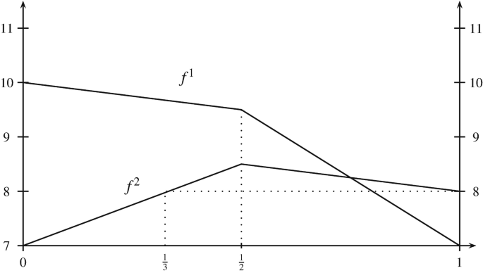

  

  Computing ${\mathscr {X}_{par}^{*}} (\{v_1,v_2\})$

  $$\displaystyle \begin{aligned}t^1=\max \left\{ t\in[0,1]:\, f^1(v_1)=f^1\left( \{v_1,v_2\},t\right)\right\}=0\end{aligned}$$
  $$\displaystyle \begin{aligned}t^2=\min \left\{ t\in[0,1]:\, f^2(v_2)=f^2\left( \{v_1,v_2\},t\right)\right\}=\frac{1}{3}\end{aligned}$$
  $$\displaystyle \begin{aligned}(\text{in } \,[0,\frac{1}{2}],\quad f^2(x) \equiv 7+3t,\, 7+3t=8 \Leftrightarrow t=\frac{1}{3})\end{aligned}$$
  $$\displaystyle \begin{aligned}{\mathscr{X}_{par}^{*}} (e)=\{v_1\}\cup\{v_2\}\cup\left( \{v_1,v_2\},\,\left(0,\frac{1}{3}\right)\right)\end{aligned}$$

• e = {v₂, v₄}. f¹(v₂) = 7 > f¹(v₄) = 6 and f²(v₂) = 8 < f²(v₄) = 9 and $B_{24}=\emptyset \Rightarrow t_1=0,\, t_2=1 \Rightarrow {\mathscr {X}_{par}^{*}} (e)={ P}(e).$

• e = {v₃, v₄}. v₄ dominates $v_3\ \Rightarrow {\mathscr {X}_{par}^{*}} (e)=\{v_4\}$.

• e = {v₁, v₃}. (Fig. 9.19) $B_{13}=\left \{ \left (\underbrace {\{v_1,v_3\}}_{b_{13}^1},\,\frac {1}{4}\right ),\left (\underbrace {\{v_1,v_3\}}_{b_{13}^2},\,\frac {3}{4}\right )\right \}$

  Fig. 9.19

  

  Computing ${\mathscr {X}_{par}^{*}} (\{v_1,v_3\})$

$$\displaystyle \begin{aligned}f\left( b_{13}^1\right)= {11.5 \choose 8.5}, \quad f\left( b_{13}^2\right)= {10.5 \choose 9.5}\end{aligned}$$

$$\displaystyle \begin{aligned}t_1=\frac{4}{5}, \quad t_2=\frac{1}{2}\end{aligned}$$

$$\displaystyle \begin{aligned}{\mathscr{X}_{par}^{*}} (e)=\{v_1\}\cup \{v_3\}\end{aligned}$$

In a second step we have to compare all local Pareto locations ${\mathscr {X}_{par}^{*}} (e),\, e\in E$ to get ${\mathscr { X}_{par}^{*}}$. With two objective functions we can map everything to the objective space where dominance can easily be computed. In the case of median objective functions on a network, we know that f¹ and f² are piecewise linear with the same potential breakpoints. This leads to the following mapping in the (z¹, z²)-space (or objective space) as shown in Fig. 9.20. Essentially, this plot shows all pairs (z₁, z₂) of the objective function values f₁(x) and f₂(x) for all points x on the edge. Again we would like to skip the technical details and proofs and refer the reader to Hamacher et al. (1999).

Fig. 9.20

Mapping ${\mathscr {X}_{par}^{*}} (e)$ to the objective space

In the objective space, a point w dominates all other points in $w+\mathbb {R}_+^2{\setminus \{0\}}:= \left \{ w+y:\, y \in \mathbb {R}_+^2{\setminus \{0\}}\right \}$ (see Fig. 9.21).

Fig. 9.21

w₁ is dominating w₂ and w₃

In order to obtain ${\mathscr {X}_{par}^{*}}$ we draw IM(f) which is defined as the set of all images of ${\mathscr {X}_{par}^{*}} (e)$ for e ∈ E in the objective space. The lower envelope for a set P of points in $\mathbb {R}^2$ is defined as

$$\displaystyle \begin{aligned}\bigcup\left\{(x,y) \in P:\, y\leq y^{\prime}\, \text{for all}\, (x,y^{\prime})\in P\right\}.\end{aligned}$$

Algorithm 9.5 (Combining the local Pareto locations)

Input: :

${\mathscr {X}_{par}^{*}} (e)$ for all e ∈ E

Step 1.:

Let $z_{\max }^1:= \max \left \{ f^1(x):\, x\in \bigcup _{e\in E}{\mathscr {X}_{par}^{*}} (e)\right \}$

Step 2.:

Build ${\mathrm{IM}(f)} =\bigcup _{e\in E} f \left ( {\mathscr {X}_{par}^{*}} (e)\right )$

Step 3.:

For each connected component l in IM(f), let $(z_l^1,\, z_l^2)$ be the right-most point (largest z¹ value) and add to IM(f) the horizontal segment going from $(z_l^1,\, z_l^2)$ to $(z_{\max }^1,\, z_l^2).$

Step 4.:

Compute the lower envelope L of IM(f), which is the lower envelope of O(|E||V |) line segments.

Step 5.:

Eliminate every horizontal line segment of L, except its left-most point.

Step 6.:

Set ${\mathscr {X}_{par}^{*}} := f^{-1}(L).$

Output: :

${\mathscr {X}_{par}^{*}}$

In order to get the same result from the dominance relation we have to add an artificial line segment and delete it from the solution (see Fig. 9.22).

Fig. 9.22

Using the lower envelope to delete dominated solutions

Steps 1 and 3 are necessary to modify IM(f) such that we can get ${\mathscr {X}_{par}^{*}}$ from the lower envelope. These steps as well as Step 2 can be done in linear time. Step 4 can be done in a naive way in $O\left ( \vert E \vert ^2\vert V \vert ^2 \right )$ or in optimal time of $O\left ( \vert E \vert \vert V \vert \log \left ( \max \left ( \vert E \vert \vert V \vert \right )\right )\right )$ by an algorithm of Hershberger (1989). Since Step 5 can be done in linear time the complexity of Step 4 determines the overall complexity. For easier handling of the segments, note that we may use instead of an open subedge $\left (\{v_i,v_j\},\,(t_1,t_2) \right )$ the closed subedge $\left (\{v_i,v_j\},\,[t_1,t_2] \right )$. After applying the algorithm we then have to test if we deleted a point directly above the left-most point (Fig. 9.23).

Fig. 9.23

Computing ${\mathscr {X}_{par}^{*}}$ for Example 9.9

Example 9.10 (Example 9.9 Cont.)

We first draw IM(f) and add the horizontal line segments. Finally, we get ${\mathscr { X}_{par}^{*}} = {P}\left (\{v_2,v_4\}\right )\cup \left ( \{v_1,v_2\}, \left . \left [ 0,\frac {1}{3} \right . \right ) \right )$.

3.1.3 Q-Criteria Case

We will now briefly explain how this approach generalizes to the Q-criteria case. Also in this situation we easily see that if for an edge e = {v_i, v_j} one endnode dominates the other one, there are no Pareto locations in the interior of e. From now on assume that neither v_i dominates v_j nor v_j dominates v_i. Let $\mathscr {Q}_1$ and $\mathscr {Q}_2$ be a partition of $\mathscr {Q}$, such that f^q(v_i) ≥ f^q(v_j) for all $q\in \mathscr {Q}_1$ and f^q(v_i) < f^q(v_j) for all $q\in \mathscr {Q}_2$. Of course, $\mathscr {Q}_1 \neq \emptyset ,\, \mathscr {Q}_1 \cap \mathscr {Q}_2 = \emptyset$ and $\mathscr {Q}_1 \cup \mathscr {Q}_2 = \mathscr {Q}$. Also in case of constant functions we get a similar result as in the bi-criteria case. Accordingly, assume that f(v_i) ≠ f(v_j) for an edge e = {v_i, v_j} and let

$$\displaystyle \begin{aligned}t^1(f^q):= \max \left\{ t\in [0,1]:\, f^q(v_i)= f^q\left( (\{v_i,v_j\},t)\right)\right\} \,\text{for }\, q\in \mathscr{Q}_1\end{aligned}$$

and

$$\displaystyle \begin{aligned}t^2(f^q):= \min \left\{ t\in [0,1]:\, f^q(v_j)= f^q \left( (\{v_i,v_j\},t)\right)\right\} \,\text{for }\, q\in \mathscr{Q}_2.\end{aligned}$$

Then (see Hamacher et al. (1999) for the details)

$$\displaystyle \begin{aligned}{\mathscr{X}_{par}^{*}} (e) = \{v_i\}\cup \{v_j\}\cup \left(\{v_i,v_j\},\, \left(\min_{q\in \mathscr{Q}_1}\left\{t^1(f^q)\right\},\, \max_{q\in \mathscr{Q}_2}\left\{t^2(f^q)\right\}\right) \right).\end{aligned}$$

For comparing the local Pareto locations, the mapping to the objective space becomes rather involved especially when we have to compute lower envelopes.

In order to compare ${\mathscr {X}_{par}^{*}} (e)$ for all e ∈ E pairwise, we use the following iterative procedure: Let $\left ( \{v_j,v_l\},\,[t_r,t_{r+1}]\right )$ be a subedge of ${\mathscr {X}_{par}^{*}} (e_l),\, e_l=\{v_j,v_l\}$ (to have closed subedges we neglect the vertices and handle first only the Pareto parts in the interior) where (t_r, t_r+1) are assumed to not include any further bottleneck points of e_l (if this is not true we subdivide the subedge further). This leads to

$$\displaystyle \begin{aligned}f^q \left( (\{v_j,v_l\},\,t)\right) = b_r^q + m_r^qt \quad \text{ for all }\quad q \in {\mathscr{Q}},\, t \in [t_r,t_{r+1}],\end{aligned}$$

i.e., all f^q are affine linear on $\left (\{v_j,v_l\},\, [t_r,\,t_{r+1}]\right ).$ Take now a closed linear subedge from another edge e_k = {v_k, v_m}, then we get $\left ( \{v_k,v_m\},\, [s_p,\,s_{p+1}]\right ) \subseteq {\mathscr { X}_{par}^{*}} (e_k)$. This leads to

$$\displaystyle \begin{aligned}f^q\left( (\{v_k,v_m\},\,s)\right) = b_p^q + m_p^qs \quad \text{ for all }\quad q \in {\mathscr{Q}},\, s\in [s_p,s_{p+1}],\end{aligned}$$

If we apply the definition of a Pareto location to these two subedges, we get that a point $\left (\{v_j,v_l\},\,t\right ),\, t\in [t_r,\,t_{r+1}]$ is dominated by some point $\left (\{v_k,v_m\},\,s\right ),\, s\in [s_p,\,s_{p+1}]$

$$\displaystyle \begin{aligned}\Leftrightarrow \quad b_p^q + m_p^qs \leq b_r^q + m_r^qt \quad \text{for all }\quad q\in \mathscr{Q},\end{aligned}$$

where at least one inequality is strict. Now we define the polyhedron

$$\displaystyle \begin{aligned}{\mathscr{F}} := \left\{ (s,t):\, m_r^qt-m_p^qs \geq b_p^q - b_r^q,\, \forall q\in \mathscr{Q}\right\} \cap \left( [s_p,\, s_{p+1}] \times [t_r,\, t_{r+1}]\right).\end{aligned}$$

We have two cases: If ${\mathscr {F}} = \emptyset$, then $\left ( \{v_j,v_l\},\,[t_r,\, t_{r+1}]\right )$ contains no point which is dominated by a point from $\left (\{v_k,v_m\},\,[s_p,\, s_{p+1}] \right )$. Otherwise, ${\mathscr {F}} \neq \emptyset$ is taken as a feasible solution of the two 2-variable linear programs

$$\displaystyle \begin{aligned}\text{LB}=\min \{t:\, (s,t)\in {\mathscr{F}} \}, \quad \text{UB}=\max \{t:\, (s,t)\in {\mathscr{F}} \}.\end{aligned}$$

Let s_LB and s_UB be the optimal values for s corresponding to LB and UB, respectively. Now we still have to check if one inequality is strict: If $b_p^q + m_p^q s_{\text{LB}} = b_r^q+ m_r^q\text{LB}$ and $b_p^q + m_p^q s_{\text{UB}} = b_r^q+ m_r^q\text{UB}$ for all $q\in \mathscr {Q}$, then there is no dominance. Otherwise ${\mathscr {X}_{par}^{*}} (e_l):= {\mathscr {X}_{par}^{*}} (e_l)\setminus \left ( \{v_j,v_l\},\, [\mathrm{LB},\, \mathrm{UB}])\right ).$ Note that this procedure works also if t_r = t_r+1 or s_p = s_p+1 (in this case, we are testing a single point).

Algorithm 9.6 (Combining local Pareto location in the Q-criteria case)

Input: :

Network as in Algorithm 9.4

Step 1.:

Determine ${\mathscr {X}_{par}^{*}} (e)$ for all e ∈ E and set ${\mathscr {X}_{par}^{*}} := \bigcup _{e\in E} {\mathscr {X}_{par}^{*}} (e)$

Step 2.:

Compare all v_i and all edges, where all $f^q,\, q \in \mathscr {Q}$ are constant

Step 3.:

For all Pareto linear subedges do a pairwise comparison as described above and reduce ${\mathscr {X}_{par}^{*}}$ accordingly.

Output: :

${\mathscr {X}_{par}^{*}}$

The complexity of this algorithm is O(|E|²|V |²Q).

3.1.4 Multicriteria Median Problems on a Tree

Many difficult problems on general networks become easier to solve if the underlying graph has a tree structure. We will show that this is also true for multicriteria problems. We relate our results with the research that has previously been done on trees and end up with a generalization of Goldman’s algorithm (see Goldman 1971a). The major concept which makes the analysis easier on trees is convexity. We first introduce this concept based on Dearing et al. (1976).

Let N = (T, ℓ) be a tree network, with T = (V, E). For two points a, b ∈ P(T) we define the line segment L[a, b] between a and b as

$$\displaystyle \begin{aligned} L[a,b] := \left\{ x \in P(T) :\; d(a,x) + d(x,b) = d(a,b) \right\}, \end{aligned}$$

which contains all points on the unique path between a and b. A subset C ⊆ P(T) is called convex, if and only if for all a, b ∈ C, L[a, b] ⊆ C.

Now let C ⊆ P(T) be convex and let $h:P(T) \rightarrow \mathbb {R}$ be a real valued function. This function h is called convex on C, if and only if for all a, b ∈ C,

$$\displaystyle \begin{aligned} h(x_{\lambda}) \le \lambda h(a) + (1-\lambda) h(b) \; , \, \forall \lambda \in [0,1] \; , \end{aligned}$$

where x_λ is uniquely defined by

$$\displaystyle \begin{aligned} d(x_\lambda,b) = \lambda d(a,b) \, \mbox{ and } \, d(x_\lambda,a) = (1-\lambda) d(a,b) \; . {} \end{aligned} $$

(9.5)

A function is called convex on T if it is convex on C = P(T). Note that it is possible to define convexity also on general networks. Then one can show that d(x, c) for c ∈ P(T) fixed is convex if and only if the underlying graph is a tree. Median and Center objective functions are convex functions on a tree (see Dearing et al. 1976).

Now let L(a, b) := L[a, b]∖{a, b}, L(a, b] := L[a, b]∖{a} and L[a, b) := L[a, b]∖{b}. We have now the following important property (a proof can be found in Hamacher et al. 1999).

Theorem 9.9

Let a, b ∈ P(T) and h := (h¹, …, h^Q) be a vector of Q objective functions, with h^q convex on T, for all $q \in \mathscr {Q}=\{1,\ldots ,Q\}$. Then the following holds:

$$\displaystyle \begin{aligned} \{a,b\} \subseteq \mathscr{X}_{par}^{*} \; \mathrm{if}\ \mathrm{and}\ \mathrm{only}\ \mathrm{if} \; L[a,b] \subseteq \mathscr{X}_{par}^{*} \; . \end{aligned}$$

For T = (V, E) and V^′⊆ V  let

$$\displaystyle \begin{aligned} W(V^{\prime}) := \left( \begin{array}{c} w^1(V^{\prime}) \\ w^2(V^{\prime}) \\ \vdots \\ w^Q(V^{\prime}) \end{array} \right) \; , \end{aligned}$$

where $w^q(V^{\prime }) := \sum _{v_i \in V^{\prime }} w_i^q$, $\forall q \in \mathscr {Q}$.

Using Theorem 9.9 together with two lemmata from Goldman (1971b) and the above definition of W(V ) we can prove the following result which paves the way for solving Q-criteria median problems on a tree.

Proposition 9.1

Let T be partitioned in such a way that T = T₁ ∪ T₂ ∪{e} and T₁ ∩ T₂ = ∅. Then W(V (T₁)) dominates W(V (T₂)) if and only if for all x ∈ P(T₁) there exists some y ∈ P(T₂) which dominates x.

Now we can state a multicriteria version of Goldman’s dominance algorithm (see Goldman 1971a). We start with a subtree containing only one leaf of the tree (check for dominance) and enlarge this subtree until we get a Pareto location using the criterion established in Proposition 9.1. This procedure is then repeated for all leaves and we end up with a subtree of all Pareto locations by using Theorem 9.9.

Algorithm 9.7 (Solving Q-criteria median problems on a tree)

Input: :

T = (V, E), with length function ℓ and node weight vectors w^q, $q \in \mathscr {Q}$.

Step 0.:

Set W := W(V )

Step 1.:

Choose a leaf v_k of T, which was not yet considered and give it the status “considered”.

Step 2.:

IF V = {v_k} Set ${\mathscr {X}_{par}^{*}} (f(V)):={\mathscr {X}_{par}^{*}} (f(T)):=\{v_k\}$ and go to Step 6

Step 3.:

Let v_l be the only node adjacent to v_k IF $(w_k^1 \ldots w_k^Q)^T < \frac {1}{2} \, W$ THEN

• $w_l^q:= w_l^q + w_k^q,\quad q=1, \ldots , Q$

• T := T ∖{v_k}

Step 4.:

IF there are any leaves left in T give them status “not considered”   and go to Step 1

Step 5.:

Set ${\mathscr {X}_{par}^{*}} (f(V)):= V(T)$, ${\mathscr {X}_{par}^{*}} (f(T)):= T$

Step 6.:

STOP

Output: :

${\mathscr {X}_{par}^{*}} (f(V))$ and ${\mathscr {X}_{par}^{*}} (f(T))$

The complexity of this algorithm is O(Q|V |). To illustrate the algorithm consider the following example:

Example 9.11

Consider the tree depicted in Fig. 9.24. We solve the following instance of a 3-criteria median problem. Let l(e) := 1, ∀e ∈ E. The weights of the nodes are given in the following table:

Fig. 9.24

Tree of Example 9.11. The bold edges and nodes indicate the set of Pareto locations

	v 1	v 2	v 3	v˙4	v 5	v 6	v 7	v 8	v 9	v 10	v 11
w 1	14	6	8	4	1	2	1	3	2	2	7
w 2	11	3	3	24	5	2	2	3	2	2	5
w 3	16	2	1	1	2	3	3	1	6	4	21

Therefore $W = \left ( \begin {array}{c} 50 \\ 62 \\ 60 \end {array} \right )$ and $\frac {1}{2} W = \left ( \begin {array}{c} 25 \\ 31 \\ 30 \end {array} \right )$.

The adjacency structure of the tree is also given in Fig. 9.24. Now we check every leaf till there is none left with status “not considered”.

• Take v₁: $w_1 =\left ( \begin {array}{c} 14 \\ 11 \\ 16 \end {array} \right )$ dominates $\frac {W}{2} =\left ( \begin {array}{c} 25 \\ 31 \\ 30 \end {array} \right )$.Therefore $w_2 := \left ( \begin {array}{c} 6+14 \\ 3+11 \\ 2+16 \end {array} \right ) = \left ( \begin {array}{c} 20 \\ 14 \\ 18 \end {array} \right )$.

By following the algorithm we delete v₈, v₇, v₆, v₅ and v₄. The actual value of w₃ is

$\left ( \begin {array}{c} 13 \\ 32 \\ 4 \end {array} \right )$.

• Take v₃: $w_3 =\left ( \begin {array}{c} 13 \\ 32 \\ 4 \end {array} \right )$ does not dominate $\frac {W}{2}$.

• Take v₁₁: $w_{11} =\left ( \begin {array}{c} 7 \\ 5 \\ 21 \end {array} \right )$ dominates $\frac {W}{2}$. Therefore $w_9 := \left ( \begin {array}{c} 9 \\ 7 \\ 27 \end {array} \right )$.

• Take v₁₀: $w_{10} =\left ( \begin {array}{c} 2 \\ 2 \\ 4 \end {array} \right )$ dominates $\frac {W}{2}$. Therefore $w_9 := \left ( \begin {array}{c} 11 \\ 9 \\ 31 \end {array} \right )$.

• Take v₉: $w_9 =\left ( \begin {array}{c} 11 \\ 9 \\ 31 \end {array} \right )$ does not dominate $\frac {W}{2}$.

Since we delete after every domination step the corresponding node from the tree according to Algorithm 9.7 and no leaf with status not considered is left we end up with

$$\displaystyle \begin{aligned} \mathscr{X}_{par}^{*} = L[v_9, v_3] \; .\end{aligned} $$

3.2 Other Multicriteria Location Problems on Networks

In the previous two subsections we presented optimal time algorithms for one facility median problems when looking for Pareto locations. We chose these two problems because the reader gets some insight into the needed properties. In addition, the simplification on trees caused by the uniqueness of paths can be seen. In survey by Nickel et al. (2005a) an overview on other location problems can be found. In Hamacher et al. (2002) an extension to 1-facility center problems as well as to positive and negative weight vectors on the nodes is developed. Those ideas have been further extended to problems with criteria dependent lengths in Skriver et al. (2004). A unified framework for multicriteria ordered median functions can be found in Nickel et al. (2005b), Nickel and Puerto (2005). In Colebrook and Sicilia (2007b) the location of undesirable facilities on multicriteria location problems on networks is looked into by using convex combinations of two objective functions. Some complexity analysis for the cent-dian location problem has been developed by Colebrook and Sicilia (2007a). Most approaches to the (in general NP-hard) multi-facility case are treated as discrete location problems (see Sect. 9.4). Only Kalcsics et al. (2015) found polynomial cases of multi-facility multicriteria location problems on networks. In Kalcsics et al. (2014), the authors discuss the multicriteria p-facility median location problem on networks with positive and negative weights; providing an efficient algorithm to solve the bicriteria 2-facility problem and a polynomial algorithm for the general problem when the number of facilities and criteria is fixed.

4 Discrete Location Problems

The previous sections show that planar and network multicriteria location problems have been widely developed from a methodological point of view so that important structural results and algorithms are known to determine solution sets. On the contrary, multicriteria analysis of discrete location problems has attracted less attention. In spite of that, several authors have dealt with problems and applications of multicriteria decision analysis in this field. An annotated bibliography with many references up to 2005 can be found in Nickel et al. (2005a). In general, very few papers focus in the complete determination of the whole set of Pareto-optimal solutions. Nevertheless, there are some exceptions, such as the paper by Ross and Soland (1980) that gives a theoretical characterization but does not exploit its algorithmic possibilities, as well as the work by Fernández and Puerto (2003) that addresses the computation of the entire set of Pareto-optimal solutions of the multiobjective uncapacitated plant location problem. The methodology developed was extended to the capacitated version by Arora and Arora (2010).

Nowadays, Multi-Objective Combinatorial Optimization (MOCO) (see Ehrgott and Gandibleux 2000, Ulungu and Teghem 1994) provides an adequate framework to tackle various types of discrete multicriteria problems such as the p-Median Problem (p-MP). Within this emergent research area, several methods are known to handle different problems. It is worth noting that most of MOCO problems are NP-hard and intractable (see Ehrgott and Gandibleux 2000, for further details). Even in most of the cases where the single objective problem is polynomially solvable the multiobjective version becomes NP-hard. This is the case of spanning tree problems and min-cost flow problems, among others. In the case of the p-MP, the single objective version is already NP-hard. This ensures that the multiobjective formulation is not solvable in polynomial time unless P= NP. In this context, when time and efficiency become a real issue, different alternatives can be used to approximate the Pareto-optimal set. One of them is the use of general-purpose MOCO heuristics (Gandibleux et al. 2000). Another possibility is the design of “ad hoc” methods based on one of the following strategies: (1) computing supported non-dominated solutions; and (2) performing partial enumerations of the solutions space. Obviously, the second strategy does not guarantee the non-dominated character of all the generated solutions although the reduction in computation time can be remarkable.

The aim of this section is to present methods to obtain the Pareto-optimal set for the multiobjective p-median problem (p-MP). In all cases, our approach to solve the multicriteria p-MP takes advantage of the problem’s structure. The first method is exact and it determines the whole set of Pareto-optimal solutions based on new tools borrowed from the theory of short rational generating functions. The second method is an “ad hoc” approximate method that generates supported Pareto locations.

4.1 Model and Notation

Let I = {1, …, M} and J = {1, …, N} respectively denote the sets of indices for demand points and for plants, and $\mathscr {Q} = \{1,\ldots , Q \}$ denote the set of indices for the considered criteria. For each criterion $q\in \mathscr {Q}$ , let $(c_{ij}^q)_{i\in I,j\in J}\in \mathbb {Q}^{M\times N}$ be the allocation costs of demand points to plants. The multicriteria p-median location problem is:

$$\displaystyle \begin{aligned} \begin{array}{rcl} &\displaystyle \mbox{v-}\mathrm{Minimize} &\displaystyle \displaystyle \left( \sum_{i=1}^M \sum_{j=1}^N c_{ij}^1x_{ij},\ldots,\sum_{i=1}^M \sum_{j=1}^N c_{ij}^q x_{ij}\right) {} \end{array} \end{aligned} $$

(9.6)

$$\displaystyle \begin{aligned} \begin{array}{rcl} &\displaystyle \mbox{subject to}&\displaystyle \displaystyle \sum_{j=1}^N x_{ij}=1, \quad i\in I, {} \end{array} \end{aligned} $$

(9.7)

$$\displaystyle \begin{aligned} \begin{array}{rcl} &\displaystyle &\displaystyle x_{ij}\le y_j, \quad i\in I,\; j\in J, {} \end{array} \end{aligned} $$

(9.8)

$$\displaystyle \begin{aligned} \begin{array}{rcl} &\displaystyle &\displaystyle \sum_{j=1}^N y_j=p, {} \end{array} \end{aligned} $$

(9.9)

$$\displaystyle \begin{aligned} \begin{array}{rcl} &\displaystyle &\displaystyle x_{ij}\in \{0,1\},\; y_j\in \{0,1\}, \quad i\in I,\; j\in J.{} \end{array} \end{aligned} $$

(9.10)

As it is usual, v-min stands for vector minimum of the considered objective functions. Here variable y_j takes the value 1 if plant j is open and 0 otherwise. The binary variable x_ij is 1 if the demand point i is assigned to plant j and 0 otherwise. Constraints (9.7), together with integrality conditions on the x variables, ensure that each demand point is assigned to exactly one plant, while constraints (9.8) guarantee that no demand point is assigned to a non-open plant. Finally, constraint (9.9) ensures that exactly p plants are opened.

Recall that in the single criterion case the integrality conditions on the x variables need not be explicitly stated. The reason is that when the x_ij represent the proportion of demand of client i satisfied by plant j (i.e. 0 ≤ x_ij ≤ 1), there exists an optimal solution with x_ij = 0, 1, i ∈ I, j ∈ J. This property is not necessarily true when multiple criteria are considered because, in general, there might be non-dominated solutions with non-integer values and even non-supported non-dominated integer solutions.

4.2 Determining the Entire Set of Pareto-Optimal Solutions

In order to characterize the set of Pareto locations of the p-MP we shall use rational generating functions. Short rational generating functions were used by Barvinok (1994) as a tool to develop an algorithm for counting the number of integer points inside convex polytopes, based on the previous geometrical paper by Brion (1988). The main idea is to encode those integer points in a rational function of as many variables as the dimension of the space where the polytope is defined. Let $P \subset \mathbb {R}^n_+$ be a given convex bounded polyhedron. Its integer points may be expressed in a formal sum f(P, z) =∑_αz^α with $\alpha = (\alpha _1, \ldots , \alpha _n) \in P\cap \mathbb {Z}^n$, where $z^\alpha = z_1^{\alpha _1}\cdots z_n^{\alpha _n}$ Barvinok’s goal was to represent that formal sum of monomials in the multivariate polynomial ring $\mathbb {Z}[z_1, \ldots , z_n]$, as a “short” sum of rational functions with the same variables. Actually, Barvinok (1994) developed a polynomial-time algorithm to compute those functions when the dimension, n, is fixed. A clear example is the polytope $P = [0,T] \subset \mathbb {R}$ with $T \in \mathbb {N}$: the long expression of the generating function of the integer points inside P is $\mathrm {f}(P,z) = \sum _{i=0}^T z^i$, and it is easy to see that its representation as sum of rational functions is the well known formula (1 − z^T+1)∕(1 − z).

The above approach, apart from counting lattice points, has been used to develop some algorithms to solve integer programming problems exactly. Specifically, De Loera et al. (2004, 2005), and Woods and Yoshida (2005) presented different methods to solve this family of problems using Barvinok’s rational function of the polytope defined by the feasible set of the given problem.

First of all, for the sake of readability, we recall some results on short rational functions for polytopes that shall be later used in our presentation. For further details the interested reader is referred to Barvinok (1994), Barvinok and Woods (2003).

Let $P = \{x \in \mathbb {R}^n: A\,x \leq b, x\geq 0\}$ be a rational polytope in $\mathbb {R}^n$. The main idea of Barvinok’s Theory was to encode the integer points inside a rational polytope in a “long” sum of monomials:

$$\displaystyle \begin{aligned}\mathrm{f}(P,z) = \displaystyle \sum_{\alpha\in P\cap\mathbb{Z}^n}\,z^\alpha, \end{aligned}$$

where $z^\alpha = z_1^{\alpha _1}\cdots z_n^{\alpha _n}$, and then to re-encode, in polynomial-time for fixed dimension, these integer points in a “short” sum of rational functions in the form

$$\displaystyle \begin{aligned}\mathrm{f}(P;z) = \displaystyle \sum_{i\in I} \varepsilon_i \dfrac{z^{u_i}}{\displaystyle \prod_{j=1}^n (1-z^{v_{ij}})}, \end{aligned}$$

where I is a polynomial-size indexing set, ε_i ∈{1, −1}, and $u_i , v_{ij} \in \mathbb {Z}^n$ for all i and j (Theorem 5.4 in Barvinok and Woods 2003).

It is well-known that enumerating the entire set of Pareto-optimal solutions of general multiobjective integer linear problems is #P-hard even in fixed dimension (see, e.g., Ehrgott and Gandibleux 2002 and Chinchuluun and Pardalos 2007). Therefore listing these solutions, in general, is hopeless. Nevertheless, one can try to represent these sets in polynomial time using a different strategy by simply encoding their elements in an efficient way. This strategy has been applied by Blanco and Puerto (2012). In that paper, it is proved that using short generating functions of rational polytopes, one can encode the whole set of Pareto-optimal solutions of MOILP in polynomial time, fixing only the dimension of the space of variables. As an application of this result we can state the following theorem.

Theorem 9.10

Assume that the number of facilities M and plants N is fixed. Then, in polynomial time, we can encode the entire set of Pareto-optimal solutions for (9.6)–(9.10) in a short sum of rational functions.

Proof

Apply Theorem 1 in Blanco and Puerto (2012) to the polytope of Problem (9.6)–(9.10). □

The combination of Theorem 9.10 and Theorem 7 in De Loera et al. (2009) results in the following theorem.

Theorem 9.11

Assume M and N are constant. There exists a polynomial-delay polynomial-space procedure to enumerate the entire set of Pareto-optimal solutions of (9.6)–(9.10).

This construction can be implemented for problems of small to medium size dimension using the open source software barvinok, see Verdoolaege (2008).

4.3 Determining Supported Pareto-Optimal Solutions

In some situations it suffices to generate the set of supported Pareto-optimal points. It is well-known that the set of supported Pareto-optimal solutions to a problem can be obtained by solving the scalarized problem for all possible values of the scalar weights in the standard Q-dimensional simplex $\varLambda ^Q=\{\lambda \in \mathbb {R}^Q: \sum _{q=1}^Q\lambda ^q=1,\; \lambda ^q\ge 0 ,\; \forall q=1,\ldots ,Q\}.$

In order to describe how to obtain these solutions in problem (9.6)–(9.10) we need to introduce some additional notation. We denote by B any feasible basis of the linear relaxation of Problem (9.6)–(9.10); and by $\overline {N}$ all the columns that are not in B. Also, abusing notation, as usual in linear programming, we shall refer to the indices determining the basis B ($\overline {N}$) in the variables and the objective function by (x, y)_B ($(x,y)_{\overline {N}}$) and c_B ($c_{\overline {N}}$), respectively.

For any λ ∈ Λ^Q, we shall denote by c(λ) = (c_ij(λ))_ij, where $c_{ij}(\lambda )=\sum _{q=1}^Q \lambda ^q c_{ij}^q$.

For each feasible basis B, consider the subdivision of the space Λ^Q induced by the hyperplanes:

$$\displaystyle \begin{aligned}\lambda^qc_B^qB^{-1}\overline{N}-\lambda^q c_{\overline{N}}^q=0, \quad q\in \mathscr{Q}.\end{aligned}$$

Next, let $\lambda _B^Q \in \varLambda ^Q$ be a parameter such that it belongs to the relative interior of one of the elements in the above subdivision and satisfies $c_B(\lambda ^Q)B^{-1}\overline {N}-c_{\overline {N}}(\lambda ^Q)\le 0$. This choice of λ^Q ensures that the problem:

$$\displaystyle \begin{aligned} \begin{array}{rcl} &\displaystyle \mathrm{Minimize} &\displaystyle \displaystyle \sum_{i=1}^M \sum_{j=1}^N c_{ij}(\lambda_B^Q) x_{ij}{} \end{array} \end{aligned} $$

(9.11)

$$\displaystyle \begin{aligned} \begin{array}{rcl} &\displaystyle \mbox{subject to}&\displaystyle \sum_{j=1}^N x_{ij}=1,\quad i\in I, {} \end{array} \end{aligned} $$

(9.12)

$$\displaystyle \begin{aligned} \begin{array}{rcl} &\displaystyle &\displaystyle x_{ij}\le y_j,\quad i\in I,\; j\in J, {} \end{array} \end{aligned} $$

(9.13)

$$\displaystyle \begin{aligned} \begin{array}{rcl} &\displaystyle &\displaystyle \sum_{j=1}^N y_j=p, {} \end{array} \end{aligned} $$

(9.14)

$$\displaystyle \begin{aligned} \begin{array}{rcl} &\displaystyle &\displaystyle x_{ij}\ge 0,\; y_j\ge 0,\quad i\in I,\; j\in J. \end{array} \end{aligned} $$

(9.15)

will identify supported Pareto-optimal solutions of the linear relaxation of Problem (9.6)–(9.10). However, these Pareto-optimal solutions may result in fractional location variables since Problem (9.11)–(9.14) is a scalarization of the continuous version of our original multiobjective location problem. To avoid this inconvenience we shall solve the binary version of (9.11)–(9.14), namely

$$\displaystyle \begin{aligned} \begin{array}{rcl} &\displaystyle \mathrm{Minimize} &\displaystyle \sum_{i=1}^M \sum_{j=1}^N c_{ij} (\lambda_B^Q) x_{ij}{} \end{array} \end{aligned} $$

(9.16)

$$\displaystyle \begin{aligned} \begin{array}{rcl} &\displaystyle \mbox{subject to}&\displaystyle \sum_{j=1}^N x_{ij}=1,\quad i\in I, {} \end{array} \end{aligned} $$

(9.17)

$$\displaystyle \begin{aligned} \begin{array}{rcl} &\displaystyle &\displaystyle x_{ij}\le y_j,\quad i\in I,\; j\in J, {} \end{array} \end{aligned} $$

(9.18)

$$\displaystyle \begin{aligned} \begin{array}{rcl} &\displaystyle &\displaystyle \sum_{j=1}^N y_j=p, {} \end{array} \end{aligned} $$

(9.19)

$$\displaystyle \begin{aligned} \begin{array}{rcl} &\displaystyle &\displaystyle x_{ij}\in \{ 0,1\},\; y_j\in \{ 0,1\}, \quad i\in I,\; j\in J. {} \end{array} \end{aligned} $$

(9.20)

Any optimal binary solution of (9.16)–(9.20) gives a supported Pareto-optimal solution of our original multiobjective location problem. Repeating the above process for all feasible basis of Problem (9.6)–(9.10) will result in a set of supported Pareto-optimal solutions for the problem.

4.4 Other References in Discrete Location Problems

In the previous two subsections, the entire set of Pareto locations is characterized using rational generating functions of integer points in polytopes and supported Pareto-optimal solutions are identified by solving binary linear problems. These approaches provide the reader with a general idea of the tools needed to characterize the set of Pareto optimal solutions in discrete location problems. Some additional references can be found in Nickel et al. (2005a). Also Farahani et al. (2010) reviews results and developments in multicriteria location problems.

In the following we list some interesting recent references in this field: Özpeynirci (2017) introduces new properties that restrict the possible locations of the non-dominated points necessary for computing the nadir points and applied this methodology to multiobjective integer location problems. Pecci et al. (2017) study the multiobjective co-design problem of optimal valve placement and operation in water distribution networks. The resulting optimization problem is a multiobjective mixed integer nonlinear optimization problem. The multi-objective competitive location problem with distance-based attractiveness for two facilities is introduced in Wang et al. (2018). The multiobjective version of the obnoxious p-median problem was studied in Colmenar et al. (2018). That paper obtains high-quality approximations to the efficient front of the bi-objective case using a Multi-Objective Memetic Algorithm. Karatas and Yakici (2018) presents a novel methodology for solving multi-objective facility location problems with the focus on public emergency service stations, considering the p-median problem, the maximal coverage location problem and the p-center problem.

5 Conclusions

In this chapter we have presented and analyzed some of the most important models of multicriteria location problems considering three different decision spaces: continuous, networks and discrete. This material provides a general overview of the state-of-the-art of the field as well as a number of references that can be used by the interested readers to go for a further analysis of the topic. Emphasis was put on an efficient (if possible) description of the whole set of Pareto locations.

References

Alzorba S, Günther C, Popovici N (2015) A special class of extended multicriteria location problems. Optimization 64(5):1305–1320
Alzorba S, Günther C, Popovici N, Tammer C (2017) A new algorithm for solving planar multiobjective location problems involving the Manhattan norm. Eur J Oper Res 258(1):35–46
Apolinário HCF, Papa Quiroz EA, Oliveira PR (2016) A scalarization proximal point method for quasiconvex multiobjective minimization. J Global Optim 64(1):79–96
Arora S, Arora SR (2010) Multiobjective capacitated plant location problem. Int J Oper Res 7(4):487–505
Barvinok A (1994) A polynomial time algorithm for counting integral points in polyhedra when the dimension is fixed. Math Oper Res 19:769–779
Barvinok A, Woods K (2003) Short rational generating functions for lattice point problems. J Amer Math Soc 16:957–979
Bhattacharya U (2018) A mathematical model for locating k-obnoxious facilities on a plane. Int J Oper Res 31(3):384–402
Blanco V, Puerto J (2012) A new complexity result on multiobjective linear integer programming using short rational generating functions. Optim Lett 6:537–543
Brion M (1988) Points entiers dans les polyèdres convexes. Ann Sci Ecole Norm S Sér 21(4):653–663
Carrizosa E, Conde E, Fernández FR, Puerto J (1993) Efficiency in Euclidean constrained location problems. Oper Res Lett 14:291–295
Chinchuluun A, Pardalos PM (2007) A survey of recent developments in multiobjective optimization. Ann Oper Res 154:29–50
Colebrook M, Sicilia J (2007a) A polynomial algorithm for the multicriteria cent-dian location problem. Eur J Oper Res 179:1008–1024
Colebrook M, Sicilia J (2007b) Undesirable facility location problems on multicriteria networks. Comput Oper Res 34:1491–1514
Colmenar J, Martí R, Duarte A (2018) Multi-objective memetic optimization for the bi-objective obnoxious p-median problem. Knowl-Based Syst 144:88–101
De Loera JA, Haws D, Hemmecke R, Huggins P, Sturmfels B, Yoshida R (2004) Short rational functions for toric algebra and applications. J Symb Comput 38:959–973
De Loera JA, Haws D, Hemmecke R, Huggins P, Yoshida R (2005) A computational study of integer programming algorithms based on Barvinok’s rational functions. Discrete Optim 2:135–144
De Loera JA, Hemmecke R, Köppe M (2009) Pareto optima of multicriteria integer linear programs. INFORMS J Comput 21:39–48
Dearing P, Francis R, Lowe T (1976) Convex location problems on tree networks. Oper Res 24:628–642
Drezner Z (1995) Facility location. In: A survey of applications and methods. Springer, New York
Durier R (1990) On Pareto optima, the Fermat-Weber problem, and polyhedral gauges. Math Program 47:65–79
Durier R, Michelot C (1985) Geometrical properties of the Fermat-Weber problem. Eur J Oper Res 20:332–343
Durier R, Michelot C (1986) Sets of efficient points in a normed space. J Math Anal Appl 117:506–528
Edelsbrunner H (1987) Algorithms in combinatorial geometry. Springer, New York
Ehrgott M (2005) Multicriteria optimization. Springer, Heidelberg
Ehrgott M, Gandibleux X (2000) A survey and annotated bibliography of multiobjective combinatorial optimization. OR Spectr 22:425–460
Ehrgott M, Gandibleux X (2002) Multiple criteria optimization. In: State of the art annotated bibliographic surveys. Kluwer, Boston
Elleuch MA, Frikha A (2018) Combining the promethee method and mathematical programming for multi-objective facility location problem. Int J Multicrit Decis Mak 7(3/4):195–216
Farahani RZ, Steadieseifi M, Asgari N (2010) Multiple criteria facility location problems: a survey. Appl Math Model 34(7):1689–1709
Fernández E, Puerto J (2003) Multiobjective solution of the uncapacitated plant location problem. Eur J Oper Res 145:509–529
Gandibleux X, Jaszkiewicz A, Freville A, Slowinski RE (2000) Special issue ‘multiple objective metaheuristics’. J Heuristics 6:291–431
Goldman A (1971a) Optimal center location in simple networks. Transport Sci 5:212–221
Goldman AJ (1971b) Optimal center location in simple networks. Transport Sci 5:212–221
Hakimi S (1964) Optimum location of switching centers and the absolute centers and medians of a graph. Oper Res 12:450–459
Hamacher H, Nickel S (1996) Multicriteria planar location problems. Eur J Oper Res 94:66–86
Hamacher HW, Labbé M, Nickel S (1999) Multicriteria network location problems with sum objectives. Networks 33:79–92
Hamacher HW, Labbé M, Nickel S, Skriver AJ (2002) Multicriteria semi-obnoxious network location problems (MSNLP) with sum and center objectives. Ann Oper Res 110:33–53
Hansen P, Perreur J, Thisse J (1980) Location theory, dominance and convexity: some further results. Oper Res 28:1241–1250
Hansen P, Labbé M, Thisse JF (1991) From the median to the generalized center. RAIRO 25:73–86
Hershberger J (1989) Finding the upper envelope of n line segments in o(\(n \log n\)) time. Inform Process Lett 33:169–174
Kalcsics J, Nickel S, Pozo MA, Puerto J, Rodríguez-Chía AM (2014) The multicriteria p-facility median location problem on networks. Eur J Oper Res 235(3):484–493
Kalcsics J, Nickel S, Puerto J, Rodríguez-Chía AM (2015) Several 2-facility location problems on networks with equity objectives. Networks 65(1):1–9
Karatas M, Yakici E (2018) An iterative solution approach to a multi-objective facility location problem. Appl Soft Comput 62:272–287
Nickel S (1995) Discretization of planar location problems. Fachbereich mathematik, PhD Dissertation, University of Kaiserslautern
Nickel S (1997) Bicriteria and restricted 2-facility weber problems. Math Method Oper Res 45:167–195
Nickel S, Puerto J (2005) Location theory: a unified approach. Springer, Berlin
Nickel S, Puerto J, Rodríguez-Chía AM (2005a) MCDM location problems. In: Figueira JA, Greco S, Ehrogott M (eds) Multiple criteria decision analysis: state of the art surveys, international series in operations research & management science, vol 78. Springer, New York, pp 761–787
Nickel S, Puerto J, Rodríguez-Chía AM, Weissler A (2005b) Multicriteria planar ordered median problems. J Optimiz Theory App 126:657–683
Özpeynirci O (2017) On nadir points of multiobjective integer programming problems. J Global Optim 69(3):699–712
Pecci F, Abraham E, Stoianov I (2017) Scalable Pareto set generation for multiobjective co-design problems in water distribution networks: a continuous relaxation approach. Struct Multidiscip Optim 55(3):857–869
Puerto J, Fernández F (1999) Multi-criteria minisum facility location problems. J Multi-Criteria Decis Anal 8:268–280
Puerto J, Fernández F (2000) Geometrical properties of the symmetrical single facility location problem. J Nonlinear Convex A 1:321–342
Rockafellar R (1970) Convex analysis. Princeton University Press, Princeton
Rodríguez-Chía A, Puerto J (2002) Geometrical description of the weakly efficient solution set for multicriteria location problems. Ann Oper Res 111:179–194
Rodríguez-Chía A, Nickel S, Puerto J, Fernández F (2000) A flexible approach to location problems. Math Method Oper Res 51:69–89
Ross GT, Soland RM (1980) A multicriteria approach to the location of public facilities. Eur J Oper Res 4:307–321
Skriver AJ, Andersen KA, Holmberg K (2004) Bicriteria network location (BNL) problems with criteria dependent lengths and minisum objectives. Eur J Oper Res 156:541–549
Ulungu E, Teghem J (1994) Multi-objective combinatorial optimization problems: a survey. J Multi-Criteria Decis Anal 3:83–104
Verdoolaege S (2008) Software barvinok. http://freecode.com/projects/barvinok
Wang SC, Lin CC, Chen TC, Hsiao H (2018) Multi-objective competitive location problem with distance-based attractiveness for two facilities. Comput Electr Eng 71:37–250
Warburton A (1983) Quasiconcave vector maximization : connectedness of the sets of pareto-optimal and weak pareto-optimal alternatives. J Optimiz Theory App 40:537–557
Weissler A (1999) General bisectors and their application in planar location theory. Shaker, Aachen
Wendell R, Hurter AJ (1973) Location theory, dominance and convexity. Oper Res 21:314–320
Wendell R, Hurter A, Lowe T (1977) Efficient points in location problems. AIIE Trans 9:238–246
Woods K, Yoshida R (2005) Short rational generating functions and their applications to integer programming. SIAG/OPT Views and News 16:15–19
Acknowledgements
The authors were partially supported by projects MTM2016-74983-C2-01/02-R (Ministry of Science, Innovation and Universities∖FEDER, Spain).
Author information
Authors and Affiliations
Corresponding author
Editor information
Editors and Affiliations
Rights and permissions
Copyright information
© 2019 Springer Nature Switzerland AG
About this chapter
Cite this chapter
Nickel, S., Puerto, J., Rodríguez-Chía, A.M. (2019). Location Problems with Multiple Criteria. In: Laporte, G., Nickel, S., Saldanha da Gama, F. (eds) Location Science. Springer, Cham. https://doi.org/10.1007/978-3-030-32177-2_9
Download citation
DOI: https://doi.org/10.1007/978-3-030-32177-2_9
Published:
Publisher Name: Springer, Cham
Print ISBN: 978-3-030-32176-5
Online ISBN: 978-3-030-32177-2
eBook Packages: Mathematics and StatisticsMathematics and Statistics (R0)