The Golden Rule Under Uncertainty

Abstract

As an English proverb goes, “Between the cup and lip a morsel may slip.” This chapter is devoted to the Golden Rule under uncertainty, which accompanies every concept of equilibrium (in particular, Berge equilibrium).

Dubia plus torquent mala.¹

As an English proverb goes, “Between the cup and lip a morsel may slip.” This chapter is devoted to the Golden Rule under uncertainty, which accompanies every concept of equilibrium (in particular, Berge equilibrium).

3.1 Uncertainty and Types of Uncertainty

L’homme propose et dieu dispose.²

The harm and good of action are conditioned by

a totality of the circumstances.

—Kozma Prutkov³

What is uncertainty? How does uncertainty appear in economic and mechanical systems, sociology and decision-making? These questions are discussed below.

3.1.1 Conceptual Meaning of Uncertainty

The following situation seems common for almost everybody: one needs to reach a place of employment from home. First of all, a person in this situation (henceforth called passenger) has to decide which means of transportation to use (subway, bus, tramcar, suburban electric train, etc.). Choosing a means of transportation (strategy), the passenger inevitably encounters incomplete and/or inaccurate information: delays or breakdowns of vehicles, sudden changes of schedule, strikes of drivers, weather fluctuations, crashes on routes, and so on. As noted by O. Holmes, “The longing for certainty…is in every human mind. But certainty is generally illusion.”⁴ At best the passenger knows the ranges of variation of these factors, without any probabilistic appraisals. Nevertheless, he/she has to make a decision! As a matter of fact, the incomplete and/or inaccurate information about the conditions under which his/her strategy will be implemented results in its inherent uncertainty. The uncertainty is caused by the embarrassment of choice.⁵ We end this section by quoting Napoleon Bonaparte: “If the art of war were nothing but the art of avoiding risks, glory would become the prey of mediocre minds…I have made all the calculations; fate will do the rest.”⁶

3.1.2 Uncertainty in Economic Systems

The following types of uncertainty are common in economic systems [25, 117, 118, 123, 125, 126, 129, 130, 175]:

• 1. uncertainty in economic indicators;

• 2. uncertainty about future disturbances, endogenous and exogenous;

• 3. uncertainty induced by mathematical modeling.

Pliny the Elder was used to say, “In these matters the only certainty is that there is nothing certain.”⁷ Among the sources and causes of uncertainty, we are identifying pure economic and also political factors. The latter include such unforeseen events as

• military conflicts and bans on exports and imports dictated by wartime (closure of borders, military operations in a country, migration, etc.);

• disposition of immovable and movable property (in particular, financial assets) on political grounds;

• inefficient economic policy and related ethnical and regional problems, polarization of different social groups.

An economic system, e.g., a firm, is often subject to sudden influence that is difficult to predict, namely, exogenous disturbances in the form of

• forces of nature (earthquakes, floods, storms, hurricanes, and other natural phenomena such as cold, ice, hail, thunder, drought, etc.);

• various accidents (fires, blasts, emissions of atomic and heat power plants, etc.);

• product price fluctuations caused by demand-supply dynamics, the varying number and range of supplies, purchase price fluctuations, the disruption of supplies;

• bad faith, low qualification or incompetence of economic partners, counteractions of rivals, acts of terrorism or racketeering;

• emergence or implementation of new technologies (investments made in technological progress and the resulting economic effects are often separated in time and therefore can be predicted on a long-term basis only);

as well as endogenous disturbances in the form of

• breakdown and failure of industrial equipment;

• unplanned additional cost and the losses of materials or energy during product storage and transportation;

• industrial accidents and employee illness;

• mistakes in personnel management;

• incorrect marketing or pricing policies (no sales, old stocks);

• mistakes in planning and product design;

• innovations suggested by employees.

New technologies and also anthropogenic and weather changes may cause uncertainty in ecological systems. In this context, we also mention epidemics among biological species and sudden pollution of their habitats [32, 147, 183].

3.1.3 Uncertainty in Mechanical Control Systems

In mechanical control systems, le vague ⁸ can be induced by exogenous disturbances, which lead to uncertainty in the forces affecting these systems [1, 107, 108, 153, 154, 169, 170, 174]. Atmospheric phenomena such as puff and varying air density can be sources of exogeneous disturbance. Incomplete information can be also a consequence of control program errors. Other disturbing factors include inaccurate initial data, the spread of characteristics and design parameters of a moving body, as well as gravitational and other perturbations. A primary cause of incomplete information in mechanical control systems consists in the inherent noises of measurement channels, which yield inaccurate motion parameters of the systems.

Information delays associated with finite periods of time needed to acquire and process measurement data also cause uncertainty in mechanical control systems.

3.1.4 Uncertainty in Decision-Making

As a matter of fact, uncertainty occurs in decision-making too.

First, in the course of mathematical modeling, since it often seems impossible to consider the whole variety of constraints on the uncontrolled and controlled parameters of the process under study within the current level and methods of science [6, 15–17, 132, 133, 135, 177, 178].

Second, in the understanding of all goals to be achieved by a controlled process: in many cases these goals are unclear or ambiguous, and their formalization has a subjective character defined by a player [7, 17, 139–142, 151].

Third, relationships between the process variables in the form of differential and/or algebraic equations may be inadequate for the process itself [9, 10, 143–146].

3.1.5 Classification of Uncontrolled Factors

In accordance with operations research [28], the strategies are the factors controlled by a player, i.e., chosen at his own discretion. Also, there exist uncontrolled factors [295, 296] affecting the outcome, which are not at the player’s disposal (e.g., environmental conditions). Obviously, players should have some information about the values of uncontrolled factors.

Based on the awareness of players, operations research [28] divides the uncontrolled factors into three groups: fixed, random, and uncertain.

The fixed uncontrolled factors are the ones that have precisely known (given) values; e.g., a share sale is transacted if the buyers are informed about the exact price quotations. In this example the price quotations act as an uncontrolled factor.

The random uncontrolled factors are represented by random variables obeying given probability distributions.

Finally, the uncertain uncontrolled factors (hereinafter referred to as uncertainty) are deterministic or random variables with given value ranges or given classes of admissible probability distributions.

Among the above-mentioned groups, of crucial importance are the random and uncertain uncontrolled factors. In fact, the fixed uncontrolled factors do not differ from the other parameters of a mathematical model: their values are given and not varied at the wish of players. The random factors and uncertainty are also not affected by the players, but they take unknown values. As a rule, the random factors have a given probability distribution. In other words, if a random factor takes a finite set of values y ₁, …, y _k, then the players know the probabilities p ₁, …, p _k associated with these values. For a random factor described by a continuous random variable, one deals with a given probability density function p(x). In both cases, the optimization criteria (payoffs functions) are defined in terms of expectation.

Even less information is available about uncertainty. Whenever it represents a deterministic variable, we will assume that there is a given domain Y of its admissible values and consider the values y ∈Y only. If uncertainty is a random variable, then by assumption it belongs to a given class of admissible probability distributions.

Modern publications on economics distinguish three types of uncertainty as follows:

• interval uncertainty, for which the only available information consists of the ranges of admissible values (any probabilistic characteristics are absent for some reason). This type of uncertainty will be studied in our book;

• random uncertainty, as discussed above;

• fuzzy uncertainty, which is ruled by fuzzy mathematics, an intensively developing branch [99] founded by L. A. Zadeh.

3.1.6 Classification of Uncertainty

Using different sources of uncertainty, it is possible to suggest four groups of uncertainty [297–300], namely,

1⁰  .:

uncertainty caused by the purposeful actions of other persons who are not players;

2⁰  .:

uncertainty reflecting the fuzzy knowledge of all players about their goals;

3⁰  .:

uncertainty occurring due to an insufficient exploration of processes or characteristics;

4⁰  .:

uncertainty arising in the course of data acquisition, processing and transfer.

Let us discuss each group in detail.

1⁰. Real control systems (especially economic, ecological, and social ones) often operate under conflict. In such systems, uncertainty is connected with the actions of conflicting parties, which are pursuing individual goals. Uncertainties of this type are called strategic [28] and cover any uncertainty caused by the actions of such goal-oriented parties actually not representing players. For example, the operation of an economic object can be influenced by other enterprises and firms, regardless of their economic relations with this object (say, an import product put in a market). These relations are incorporated into a mathematical model using several parameters with given ranges of variation (as the only information available to the players), e.g., the minimal and maximal quantity of products released in the market by an importer. The specific values of these parameters depend on the specific actions of other enterprises, i.e., the importer.

In this case, the parameters themselves constitute the uncertainty. Besides, this type of uncertainty also covers some exogenous disturbances such as the disruption and variation of the quantity (range) of supply, demand fluctuations for the products supplied by a given enterprise, the emergence of new technologies, etc.

2⁰. A special status is assigned to the uncertainty that reflects the player’s understanding of his goals. Roughly speaking, this uncertainty is not a controlled factor because each player chooses goals at his wish. However, if a player is unable to make choices or has some doubts, the resulting situation resembles the case of uncontrolled factors. For further analysis, we will assume that such a situation can be described by a set of criteria f ₁(x),…, f _N(x), each maximized by a given player without a clear view of a single criterion. As demonstrated below, this player operates under the same conditions as uncontrolled factors. A similar state of affairs occurs if the player’s criterion depends on the uncertainty taking a finite set of values: substituting these values into the criterion, we obtain a vector criterion with the same number of components as the number of uncertainty values.

Of course, an immediate issue is to design a uniform scalar criterion that would reflect the “desires” associated with all the elements of the vector criterion (the criteria convolution problem). The most widespread methods to convolute the criteria f ₁(x),…, f _N(x) are (a) the weighted sum $\sum _{i=1}^N \alpha _if_i(x)$ and (b) the weighted minimum $\min \limits _{1\leqslant i\leqslant N} \alpha _if_i(x)$. In both cases, the weight coefficients must often satisfy the normalization conditions $\sum _{i=1}^N\alpha _i=1$, where α _i > 0 (i = 1, …, N). These coefficients can be used to transform the results into a universal measuring scale. Inaccurate knowledge about the player’s goal is encoded by the uncertain values of α _i (i = 1, …, N).

However, such an approach, first, does not eliminate the existing uncertainty (yielding the uncertain parameters α _i) and, second, can be used if the uncertainty takes a finite set of values. If this set is infinite or even has the cardinality of the continuum, then the approach is called into question.

Finally, the relationship between the criterion values and uncertainty can be determined by different factors such as weather conditions, anthropogenic changes, a sudden appearance of competitors, price fluctuations in the market, and other exogenous disturbances [81,82,305].

3⁰. An increasing amount of information, and consequently a rising number of studied objects (in particular, their gradual complication), is also increasing the existing uncertainty due to an insufficient exploration of processes and characteristics, compelling us emere catullum in sacco.⁹

The growing uncertainty describes well the fact that, in the course of development, any fundamental or applied science¹⁰ is posing many more problems than it actually solves. Decision-making based on incomplete data can be interpreted as conflict with nature. Note that this source of uncertainty has a subjective character in some sense. Indeed, such uncertainty depends on accumulated experience, the completeness of modern scientific knowledge, and access to new information. For example, flight missions to Mars are intended to eliminate blanks in what is known about this planet and will surely lead to new unexpected problems. The same applies to the appearance of new technologies.

4⁰. Data acquisition, processing and transfer directly involve computers for different calculations. In practice, we have to be content with approximate solutions, reconciling ourselves with the element of uncertainty in the solutions. Rough information occurs as the result of many factors—computational errors, inaccurate data transfer as well as the limited precision of numerical representations and measurements, to name a few.

Solutions obtained by a numerical method are always approximate. There exist several sources of errors for numerical solutions, such as disagreement between a mathematical model and the real phenomenon,¹¹ inaccurate initial data, and imprecision of numerical methods (e.g., roundoff errors for arithmetical and other operations).

Even hand calculation [179] involves the roundoff effect, which is associated with a finite number of decimals used for different operations. This problem is equally important for computer systems and people.

There are several reasons explaining this situation.

First, the amount of computational job that can be performed manually is considerably smaller compared with that of modern computer systems.

Second, hand calculation allows us to observe roundoff effects and undertake necessary measures for avoiding mistakes.

Third, hand calculation often employs variable-length numbers, which are adjusted to eliminate rough errors; by contrast, computer calculation deals with floating-point numbers of fixed length.

Fourth, hand calculation allows us to estimate the maximal error induced by rounding. Such estimation is very costly for computer calculation, requiring the use of statistical estimates.

Practical calculations have led to several popular methods to use computer systems for error detection and estimation. The latter is vital: prior to writing programs for a computer system, one needs to assess the expected accuracy.

Perhaps, the simplest and most successful approach to the roundoff problem is to define the range of admissible values. Then each quantity can be described by two values, i.e., the maximal and minimal ones. In a certain sense, each quantity is replaced by a range that covers its exact value. Different operations on quantities correspond to new ranges defined from the original ranges using appropriate rounding. Therefore, each stage of calculations has reliable limits for the correct value of a given quantity. These issues form the content of interval analysis [187, 256].

A direct application of interval methods in calculation processes allows us to impose limits on the solutions of problems with initial data belonging to given ranges. The resulting intervals also incorporate the roundoff errors caused by calculations. For precise initial data, these intervals contain the exact solution of an original problem and hence interval analysis gives the approximation and roundoff errors.

To pursue the path of two-sided estimation is a very promising approach, as it solves the issue of resulting errors. Two-sided estimation is proceeding with the so-called interval arithmetics [187], which operates with intervals instead of values. More specifically, it is assumed that initial data, intermediate calculations and final results belong to some intervals. Thus, a main element of interval calculus is an interval [a, b] (also termed range) defined as a set of real values x such that $\{x\in \mathbb {R} |a\leqslant x\leqslant b\}$.

Generally, when a value x is specified for computer systems, it is assumed that x incorporates an error. In terms of interval analysis, this means that in a computer system a value x belongs to an interval.

With an interval algorithm used for solving a posed problem, we may construct an interval function that contains the exact solution. In this case, the accuracy of the resulting solution is taken into account and it is also possible to perform a prior analysis of roundoff errors.

Thus, we have presented a list of factors causing uncertainty in different systems, which does not claim to be exhaustive. But this brief discussion demonstrates that uncertainty should be considered for the elementary and difficult problems, particularly, for conflicts, in which the interests of many parties are clashing with one another and undergoing the influence of uncertain disturbances. Even in simple market problems these disturbances might not be neglectable. How can one account for them in noncooperative games under uncertainty (NGU), especially in dynamic (time-varying) controlled systems? A possible approach based on an appropriate modification of the principle of guaranteed result [28, 29] was developed for multicriteria choice problems in [295] and for conflicts in [51, 289]. An alternative framework using the principle of minimax regret [267, 268] is presented in the book [66] (though for the noncooperative setup only).

In the mathematical models of CGUs, the influence of several uncertain factors is assessed by the specific values y ₁, …, y _m of corresponding scalar parameters. These values y _j (j = 1, ..., m) describe for instance the quantity of imported products (put in the market), their unit price, the number of people suffered from an accident or fire, the delays of negotiated supplies, and so on. We will also adopt a column vector y = (y ₁, …, y _m), with a set of values denoted by $\mathrm {Y}\subset \mathbb {R}^m$.

Our book addresses uncertainties that cannot be described by statistical methods. This situation occurs at least in two cases as follows:

• the probabilistic characteristics of uncertainty exist in principle, but statistical data are not available (e.g., sudden anthropogenic accidents like the Chernobyl and Fukushima Daiichi nuclear disasters) or are very expensive to acquire;

• the uncertainty y does not have any probability distribution.

The uncertainty of the second type is well illustrated by the following example; for details see [18, p. 21]. For a clothing factory, production planning for a next year heavily affects future profits, which in turn depends on the length y of women’s skirts. However, taking into account the vagaries of fashion and female logic dictating fashion trends, any probabilistic characteristics for the parameter y would be hardly expected. All one can do is to establish some obvious limits of length variations. In [18, p. 21], E. Ventsel’ called such uncontrollable factors ill uncertainty due to an unpredictable character of their specific realization. This type of uncertainty will be considered below.

Once again, we emphasize that recent publications on competitive economics have identified three types of uncertainty, namely, interval uncertainty (studied in this book), random uncertainty (based on some probabilistic characteristics of a variable y distributed on a set Y), and fuzzy uncertainty (based on the concept of a fuzzy set introduced by Zadeh in [99]).

Thus, throughout this chapter it will be assumed that the players make their decisions using a value set Y of uncertain parameters y only, i.e., there exist no probability characteristics for y. Therefore, choosing their strategies, the players are expecting any realization of y from the set Y.

3.2 General Notions and Obtained Results

3.2.1 Saddle Point and Maximin

Maximin is the problem of finding the minimum amount of

fabric required for sewing a maxi skirt.¹²

A single-criterion choice problem under uncertainty (SCPU) is described by a triplet

$$\displaystyle \begin{aligned} \langle \: \mathrm{X}_1, \mathrm{Y}, f_1(x_1,y) \: \rangle, {} \end{aligned} $$

(3.2.1)

where $\mathrm {X}_1 \subseteq \mathbb {R}^n$ denotes the set of alternatives x ₁ selected by a decision maker (DM); $\mathrm {Y} \subseteq \mathbb {R}^m$ is the set of uncertain factors y; finally, f ₁(x ₁, y) is an objective function defined on X₁ ×Y that is maximized by the DM under any realization of y ∈Y.

For problem (3.2.1), game theory considers at least two types of solutions:

• first, the saddle point $(x^0_1,y^0) \in \mathrm {X}_1 \times \mathrm {Y}$, which is defined by the equalities

  $$\displaystyle \begin{aligned} \max\limits_{x_1\in\mathrm{X}_1} f_1\left(x_1,y^0\right) = f_1\left(x^0_1,y^0\right) = \min\limits_{y\in\mathrm{Y}} f_1\left(x^0_1,y\right); {} \end{aligned} $$

  (3.2.2)

• second, the maximin $f^{\mathrm {g}}_1$ and the maximin alternatives $x^{\mathrm {g}}_1\in \mathrm {X}_1$ suggested by A. Wald [282] in 1939, which are given by

  $$\displaystyle \begin{aligned} f^{\mathrm{g}}_1 = \min\limits_{y\in\mathrm{Y}} f_1\left(x^{\mathrm{g}}_1,y\right) = \max\limits_{x_1\in\mathrm{X}_1} \min\limits_{y\in\mathrm{Y}} f_1(x_1,y). {} \end{aligned} $$

  (3.2.3)

Remark 3.2.1

The chain of equalities (3.2.2) will be used below to formalize the guaranteed balanced equilibrium as a solution concept for the noncooperative N-player game under uncertainty (NGU), the first type of the guaranteed equilibria developed in this book.

3.2.2 Auxiliary Results from Operations Research, Theory of Multicriteria Choice and Game Theory

Some background material from operations research, theory of multicriteria choice and game theory (Nash and Berge equilibria) is provided.

Operations Research

Whilst we deliberate how to begin a thing,

it grows too late to begin it.

—Quintilian

Here we present some auxiliary results from operations research, multicriteria choice problems and noncooperative games. The following fact was established in [14, p. 160].

Proposition 3.2.1

Assume that

1⁰ .:

the scalar function F(x, y) is continuous on the product of compact sets $\mathrm {X} \subset \mathbb {R}^n$ and $\mathrm {Y} \subset \mathbb {R}^m$, where Y is also convex;

2⁰ .:

for each x ∈X, the function F(x, y) is strictly convex in y on the set Y, i.e., for each x ∈X and any y ⁽¹⁾, y ⁽²⁾ ∈Y,

$$\displaystyle \begin{aligned}F\left(x,\alpha y^{(1)} + (1-\alpha) y^{(2)}\right) < \alpha F\left(x,y^{(1)}\right) + (1-\alpha)F\left(x,y^{(2)}\right) \end{aligned}$$

for any α ∈ (0,  1).

Then the m-dimensional vector function y(x) : X →Y defined by

$$\displaystyle \begin{aligned} \min\limits_{y\in\mathrm{Y}} F(x,y) = F(x,y(x)) \;\;\; \forall x \in \mathrm{X} {} \end{aligned} $$

(3.2.4)

is also continuous.

Theory of Multicriteria Choice

Vom Himmel fordert er

Die schönsten Sterne –

Und von der Erde

—Jede höchste Lust.¹³

We provide some background material from the theory of multicriteria choice that will be needed below. For two vectors $f^{(k)}=(f^{(k)}_1, \ldots , f^{(k)}_N)$ (k = 1,  2), introduce the notations:

$$\displaystyle \begin{aligned} \begin{array}{l} \left[f^{(1)} = f^{(2)}\right] \Longleftrightarrow \left[f_i^{(1)} = f_i^{(2)} \;\; (i\in \mathbb{N})\right]; \\ \left[f^{(1)} \neq f^{(2)}\right] \Longleftrightarrow \rceil \left(f^{(1)} = f^{(2)}\right); \\ \left[f^{(1)} \geqslant f^{(2)}\right] \Longleftrightarrow \left[f_i^{(1)} \geqslant f_i^{(2)} \;\; (i\in \mathbb{N})\right]; \\ \left[f^{(1)} \geq f^{(2)}\right] \Longleftrightarrow \left(f^{(1)} \geqslant f^{(2)}\right) \; \wedge \; \left(f^{(1)} \ne f^{(2)}\right); \\ \left[f^{(1)} \not \geq f^{(2)}\right] \Longleftrightarrow \rceil \left(f^{(1)} \geq f^{(2)}\right); \\ \left[f^{(1)} > f^{(2)}\right] \Longleftrightarrow \left[f_i^{(1)} > f_i^{(2)} \;\; (i\in\mathbb{N})\right]; \\ \left[f^{(1)} \ngtr f^{(2)}\right] \Longleftrightarrow \rceil \left(f^{(1)} > f^{(2)}\right). \end{array} {} \end{aligned} $$

(3.2.5)

In the sequel, an n-dimensional vector x ∈X will be called an alternative, while an m-dimensional vector y ∈Y will be called an uncertain factor, more specifically, a pure uncertainty if y ∈Y and a counter-situation if y(⋅) ∈Y^X, where Y^X denotes the set of all m-dimensional vector functions y(x) defined on the set X and taking values in the set Y. Further analysis will be confined to the counter-situations y(⋅) : Y →X that are continuous on X, i.e., y(⋅) ∈ C(X, Y).

Definition 3.2.1

For an N-criteria choice problem Γ = 〈 Y, f(x, y) 〉 with a fixed alternative x ^∗∈X,

• (a) a pure uncertainty y _S ∈Y is Slater minimal in Γ if

  $$\displaystyle \begin{aligned}f(x^*,y) \nless f(x^*,y_S) \;\;\; \forall \: y \in \mathrm{Y}; \end{aligned}$$

• (b) a pure uncertainty y _P ∈Y is Pareto minimal in Γ if

  $$\displaystyle \begin{aligned}f(x^*,y) \nleq f(x^*,y_{\mathrm{P}}) \;\;\; \forall \: y \in \mathrm{Y}. \end{aligned}$$

  For an N-criteria choice problem Γ(x) = 〈 Y^X, f(x, y) 〉 that is defined for all x ∈X,

• (c) a counter-situation y _S(x) ∈Y^X is Slater minimal if, for each x ∈X,

  $$\displaystyle \begin{aligned}f(x,y) \nless f(x,y_{\mathrm{S}}(x)) \;\;\; \forall \: y \in \mathrm{Y}; \end{aligned}$$

• (d) a counter-situation y _P(x) ∈Y^X is Pareto minimal if, for each x ∈X,

  $$\displaystyle \begin{aligned}f(x,y) \nleq f(x,y_{\mathrm{P}}(x)) \;\;\; \forall y\in \mathrm{Y}. \end{aligned}$$

Proposition 3.2.2

• (a) If in the problem Γ(x ^∗) = 〈 Y, f(x ^∗, y) 〉 the set Y is compact and the function f(x ^∗, y) is continuous on Y, then the set Y_S of Slater-minimal pure uncertainties y _S is nonempty and compact [ 152, p. 137].

• (b) The pure uncertainty y _S ∈Y that satisfies the condition

  $$\displaystyle \begin{aligned} \min\limits_{y\in\mathrm{Y}} \sum_{i\in\mathbb{N}} \alpha_i f_i(x^*,y) = \sum_{i\in\mathbf{N}} \alpha_i f_i(x^*,y_{\mathrm{S}}) {} \end{aligned} $$

  (3.2.6)

  for some $\alpha _i = {\mathrm{const}} \geqslant 0$ and $\sum \limits _{i\in \mathbb {N}} \alpha _i > 0$ is Slater minimal in the problem Γ(x ^∗) [ 152, p. 68–69].

• (c) The pure strategy y _P ∈Y that satisfies

  $$\displaystyle \begin{aligned} \min\limits_{y\in\mathrm{Y}} \sum_{i\in\mathbb{N}} \alpha_i f_i(x^*,y) = \sum_{i\in\mathbb{N}} \alpha_i f_i(x^*,y_{\mathrm{P}}) {} \end{aligned} $$

  (3.2.7)

  for some $\alpha _i \!=\! \mathrm {const} \!> \!0$ $(i\!\in \!\mathbb {N})$ is Pareto minimal in the problem Γ(x ^∗) [ 152, p. 71].

• (d) In addition, it follows from (3.2.5) that the set Y_S ⊇Y_P of Slater-minimal uncertainties is the set of the Pareto-minimal pure uncertainties y _P in the problem Γ(x ^∗).

Nash Equilibrium

On ne peut pas savoir

tout, il faut se conten-

ter de comprendre.¹⁴

Now, consider a noncooperative N-player game of the form

$$\displaystyle \begin{aligned} \langle \: \mathbb{N}, \{\mathrm{X}_i\}_{i \in \mathbb{N}}, \{f_i[x]\}_{i\in\mathbb{N}} \: \rangle, {} \end{aligned} $$

(3.2.8)

where $\mathbb {N} = \{1,\ldots ,N\}$ denotes the set of players and $\mathrm {X}_i \!\subseteq \!\mathbb {R}^{n_i}$ is the set of pure strategies x _i of player i $(i\!\in \!\mathbb {N})$.

In game (3.2.8), the players do not build any coalitions and each player i chooses his strategy x _i ∈X_i simultaneously with the other players, which yields a strategy profile $x=(x_1,\ldots ,x_N)\in \mathrm {X} = \prod \limits _{i\in \mathbb {N}}\mathrm {X}_i$. A scalar payoff function f _i[x] of player i is a priori defined on the set $\mathrm {X} \subseteq \mathbb {R}^{n}$ $(n= \sum _{i\in \mathbb {N}} n_i)$; its value in a specific strategy profile gives the payoff of player i. At a conceptual level, each player i in game (3.2.8) seeks for choosing a strategy x _i ∈X_i that would maximize his payoff in a specific strategy profile x.

In 1949, J. Nash formalized a solution of game (3.2.8), suggesting a strategy profile known today as Nash equilibrium; see [257].

Definition 3.2.2

A strategy profile $x^{\mathrm {e}}=(x^{\mathrm {e}}_1,\ldots ,x^{\mathrm {e}}_N) \in \mathrm {X}$ is called a Nash equilibrium in game (3.2.8) if

$$\displaystyle \begin{aligned}\max\limits_{x_i \in \mathrm{X}_i} f_i [x^{\mathrm{e}}||x_i] = f_i[x^{\mathrm{e}}] \;\;\; (i\in\mathbb{N}); \end{aligned}$$

as before, $[x^{\mathrm {e}}||x_i] = [x^{\mathrm {e}}_1,\ldots ,x^{\mathrm {e}}_{i-1},x_i,x^{\mathrm {e}}_{i+1},\ldots ,x^{\mathrm {e}}_N]$.

Remark 3.2.2

In accordance with Definition 3.2.2, for compact sets X_i and continuous payoff functions f _i[x] on X, the set X^e of all Nash equilibria in game (3.2.8) is a compact (possibly empty) subset of X [51, p. 174].

The next result was proved in [22, p. 93] using Brouwer’s fixed-point theorem.

Theorem 3.2.1

Consider game (3.2.8) under the assumptions that

$\left (1^{\circ }\right )$ :

the sets X_i are convex and compact;

$\left (2^{\circ }\right )$ :

each payoff function f _i[x] is continuous on X and concave in the variable x _i for any fixed values of the other variables $(i \in \mathbb {N})$.

Then there exists a Nash equilibrium in this game.

Now, consider a game (3.2.8) in which the sets X_i are compact and the payoff functions f _i[x] are continuous on X. Associate with this game (3.2.8) its mixed extension

$$\displaystyle \begin{aligned} \langle \: \mathbb{N}, \{\nu_i\}_{i \in \mathbb{N}}, \{f_i[\nu]\}_{i\in\mathbb{N}} \: \rangle, {} \end{aligned} $$

(3.2.9)

where $\mathbb {N}$ is the same as in (3.2.8); {ν _i} denotes the set of mixed strategies of player i, i.e., each ν _i(⋅) represents a probability measure—a nonnegative scalar countably-additive function defined on the Borel σ-algebra of all subsets of the compact set X_i that is normalized by unity; ν(dx) = ν ₁(dx ₁)…ν _N(dx _N) is the product measure; {ν} designates the set of all mixed strategy profiles ν(⋅); finally, the payoff function of player i in game (3.2.9),

$$\displaystyle \begin{aligned}f_i[\nu] = \int\limits_{\mathrm{X}} f_i[x] \nu(dx) = \int\limits_{\mathrm{X}_1} \cdots \int\limits_{\mathrm{X}_N} f_i[x] \nu_N(dx_N) \cdots \nu_1(dx_1), \end{aligned}$$

is defined as the expectation f _i[x] for the payoff function of game (3.2.8) (using Fubini’s theorem on switching the order of integration).

Definition 3.2.3

A mixed strategy profile ν ^e(⋅)  ∈ {ν} is called a Nash equilibrium in game (3.2.9) if

$$\displaystyle \begin{aligned}\max\limits_{\nu_i(\cdot) \in \{\nu_i \}} f_i[\nu^{\mathrm{e}}||\nu_i] = f_i[\nu^{\mathrm{e}}] \;\;\; (i\in\mathbb{N}), \end{aligned}$$

where $\nu ^{\mathrm {e}}||\nu _i = \nu ^{\mathrm {e}}_1(dx_1) \ldots \nu ^{\mathrm {e}}_{i-1}(dx_{i-1}) \nu _i(dx_i) \nu ^{\mathrm {e}}_{i+1}(dx_{i+1}) \cdots \nu ^{\mathrm {e}}_{N}(dx_{N})$ and $\nu ^{\mathrm {e}}(dx) = \nu ^{\mathrm {e}}_1(dx_1) \cdots \nu ^{\mathrm {e}}_{N}(dx_{N})$.

The following result was obtained in [22, p. 117–119] using Gliksberg’s fixed-point theorem.

Theorem 3.2.2

Consider game (3.2.8) under the assumptions that the sets X_i are convex and compact and the payoff functions f _i[x] are continuous on $\mathrm {X} = \prod \limits _{i\in \mathbb {N}} \mathrm {X}_i$. Then in this game there exists a mixed strategy Nash equilibrium.

We conclude this section with an English translation of a remarkable quote from the book [10, p. 170]: “Intuition is not adapted to comprehend gaming opposition…Mixed strategies and Nash equilibrium are two revolutionary concepts that are described in each textbook, yet remain in the shadow of world view.”

The next section introduces one possible concept of guaranteed equilibrium in a noncooperative game under uncertainty and establishes its existence in mixed strategies under standard assumptions of mathematical game theory.

Berge Equilibrium

As the call, so the echo.

—Russian proverb [127]

In 1994, V. Zhukovskiy and his postgraduate K. Vaisman formalized the Berge equilibrium as a solution concept for game (3.2.8); see the publications [11, 12, 302].

Definition 3.2.4

A strategy profile $x^{\mathrm {B}}=(x^{\mathrm {B}}_1,\ldots ,x^{\mathrm {B}}_N) \in \mathrm {X}$ is called a Berge equilibrium in game (3.2.8) if

$$\displaystyle \begin{aligned}\max\limits_{x \in \mathrm{X}} f_i \left[x||x^{\mathrm{B}}_i\right] = f_i\left[x^{\mathrm{B}}\right] \;\;\; (i\in\mathbb{N}), \end{aligned}$$

where $[x||x^{\mathrm {B}}_i] = [x_1,\ldots ,x_{i-1},x^{\mathrm {B}}_i,x_{i+1},\ldots ,x_N]$.

Theorem 3.2.1 and Property 2.6.1 directly imply

Proposition 3.2.3

Consider game (3.2.8) with $\mathbb {N} = \{1,2\}$ under the assumptions that, for each i = 1,  2,

$\left . (1^{\circ } \right )$ :

the sets X_i are convex and compact;

$\left . (2^{\circ } \right )$ :

the payoff functions f _i[x] (i = 1,  2) are continuous on X, f ₁[x] is concave in x ₂ and f ₂[x] concave in x ₁ for each fixed strategy of the other player.

Then there exists a Berge equilibrium in this game.

Denote by X^B the set of all Berge equilibria in game (3.2.8). By Property 2.3.1, X^B is a (possibly, empty) compact set if the payoff functions f _i[x] are continuous and the sets X_i $(i \in \mathbb {N})$ are compact.

Definition 3.2.5

A strategy profile x ^∗∈X is called a Berge–Pareto equilibrium in game (3.2.8) if

first, x ^∗ is a Berge equilibrium in $(\!3.2.8)$, i.e.,

$$\displaystyle \begin{aligned}\max\limits_{x_i \in \mathrm{X}_i} f_i [x^*||x_i] = f_i[x^*] \;\;\; (i\in\mathbb{N}), \end{aligned}$$

and second, x ^∗ is a Pareto-maximal alternative in the N-criteria choice problem

$$\displaystyle \begin{aligned}\langle \: \mathrm{X}^{\mathrm{B}}, \{f_i[x]\}_{i\in\mathbb{N}} \: \rangle, \end{aligned}$$

i.e., for all x ∈X^B, the system of inequalities

$$\displaystyle \begin{aligned}f_i[x] \geqslant f_i[x^{*}] \;\;\; (i\in\mathbb{N}), \end{aligned}$$

with at least one strict inequality, is inconsistent.

Now, let us pass to the mixed extension (2.9.1) of game (3.2.8) (see Sect. 2.9.1).

Definition 3.2.6

A mixed strategy profile ν ^∗(⋅)  ∈ {ν} is called a Berge–Pareto equilibrium in mixed strategies in game (3.2.9) (equivalently, a Berge–Pareto equilibrium in the mixed extension of game (3.2.8)) if

first, ν ^∗(⋅) is a Berge equilibrium in game (2.9.1), i.e., conditions (2.9.2) are satisfied,

and second, ν ^∗(⋅) is a Pareto-maximal alternative in the N-criteria choice problem

$$\displaystyle \begin{aligned}\langle \{\nu^{\mathrm{B}}\}, \{f_i[\nu]\}_{i \in \mathbb{N}} \rangle, \end{aligned}$$

i.e., for all ν(⋅) ∈{ν ^B} the system of inequalities

$$\displaystyle \begin{aligned}f_i[\nu] \geqslant f_i[\nu^{*}] \;\;\; (i \in \mathbb{N}), \end{aligned}$$

with at least one strict inequality, is inconsistent.

The following result is a stronger analog of Theorem 3.2.2, which was proved in Sect. 2.9.3.

Theorem 3.2.3

If in game (3.2.8) the sets $\mathrm {X}_i \in \mathrm {comp} \:\mathbb {R}^{n_i}$ and the functions f _i[⋅] ∈ C(X) $(i \in \mathbb {N})$, then this game possesses a Berge–Pareto equilibrium in mixed strategies.

3.3 Balanced Equilibrium as an Analog of Saddle Point

Faber est suae quisque fortunae.¹⁵

3.3.1 Analogs of Saddle Point: The Idea and Formalization

Nothing obstructs seeing as much as a viewpoint.

—Don-Aminado¹⁶

The concept of a Slater-guaranteed balanced Berge equilibrium is formalized for the noncooperative N-player game under uncertainty.

As a matter of fact, the first type of equilibrium discussed below was suggested by V. Zhukovskiy in 1994 in the book [93, p. 233] for noncooperative games under uncertainty and later used by him for different types of equilibria [56] and also for cooperative games [52]. The whole idea is very simple: replace minimization in (3.2.2) by a vector minimum (in the sense of Slater, Pareto, Borwein, Geoffrion, or the A-minimum [295]) and replace maximization by an equilibrium design (in the sense of Nash, Berge, threats and counter-threats, or active equilibrium [54]). This approach was employed by K. Vaisman in a series of publications [280, 281]. One of his concepts will be presented below in Definition 3.3.1.

Consider a noncooperative N-player game with pure strategies and pure uncertainties, defined by

$$\displaystyle \begin{aligned} \langle \: \mathbb{N}, \{\mathrm{X}_i\}_{i \in \mathbf{N}}, \mathrm{Y}, \{f_i(x,y)\}_{i\in\mathbf{N}} \: \rangle. {} \end{aligned} $$

(3.3.1)

In (3.3.1), $\mathbb {N} = \{ 1, \ldots , N \}$ denotes the set of players; $\mathrm {X}_i \subseteq \mathbb {R}^{n_i}$ is the set of pure strategies x _i of player i; $\mathrm {Y} \subseteq \mathbb {R}^{m}$ gives the set of pure uncertainties y.

In this game, no coalitions are allowed and each player i chooses his strategy x _i simultaneously with the other players, which yields a strategy profile $x=(x_1,\ldots ,x_N)\in \mathrm {X} = \prod _{i\in \mathbb {N}}\mathrm {X}_i$. Regardless of their choice, some pure uncertainty y ∈Y arises in game (3.3.1). For each player i $(i\in \mathbb {N})$, a payoff function f _i(x, y) is defined on all such pairs (x, y) ∈X ×Y.

At a conceptual level, each player i in game (3.3.1) chooses a pure strategy x _i ∈X_i in order to maximize his payoff f _i(x, y) under any unpredictable realization of the pure uncertainty y ∈Y.

Definition 3.3.1

A pair $(\bar {x}^{\mathrm {B}},\bar {f}^{\mathrm {S}}) \in \mathrm {X} \times \mathbb {R}^N$ is called a Slater-guaranteed balanced Berge equilibrium in game (3.3.1) if there exists an uncertain factor y _S ∈Y such that

$\left .(1^{\circ }\right )$ :

the pure strategy profile x ^B is a Berge equilibrium in the game

$$\displaystyle \begin{aligned} \langle \: \mathbb{N}, \{\mathrm{X}_i\}_{i \in \mathbb{N}}, \{f_i(x,y_{\mathrm{S}})\}_{i\in\mathbb{N}} \: \rangle {} \end{aligned} $$

(3.3.2)

(which is obtained from (3.3.1) by setting y = y _S), i.e., by Definition 3.2.4,

$$\displaystyle \begin{aligned} \max\limits_{x \in \mathrm{X}} f_i \left(x||x^{\mathrm{B}}_i,y_{\mathrm{S}}\right) = f_i\left(x^{\mathrm{B}},y_{\mathrm{S}}\right) \;\;\; (i\in\mathbb{N}); {} \end{aligned} $$

(3.3.3)

$\left .(2^{\circ }\right )$ :

the uncertain factor y _S is Slater minimal in the N-criteria choice problem

$$\displaystyle \begin{aligned} \langle \: \mathrm{Y}, \{f_i\left(x^{\mathrm{B}},y\right)\}_{i\in\mathbb{N}} \: \rangle {} \end{aligned} $$

(3.3.4)

(which is obtained from (3.3.1) by setting x = x ^B), i.e., by Definition 3.2.1,

$$\displaystyle \begin{aligned} f\left(x^{\mathrm{B}},y\right) \nless f\left(x^{\mathrm{B}},y_{\mathrm{S}}\right) \;\;\; \forall y \in \mathrm{Y}; {} \end{aligned} $$

(3.3.5)

$\left .(3^{\circ }\right )$ :

the pair $(\bar {x}^{\mathrm {B}},\bar {y}_{\mathrm {S}})$ is Slater-maximal in the N-criteria choice problem

$$\displaystyle \begin{aligned} \left \langle \: \left\{ x^{\mathrm{B}},y_{\mathrm{S}} \right \}, \{f_i(x,y)\}_{i\in\mathbb{N}} \: \right \rangle {} \end{aligned} $$

(3.3.6)

(in which each element (x ^B, y _S) of the set {x ^B, y _S} satisfies (3.3.3) and (3.3.5)), i.e., the vector

$$\displaystyle \begin{aligned} \bar{f}^{\mathrm{S}} = f\left(\bar{x}^{\mathrm{B}},\bar{y}_{\mathrm{S}}\right) \nless f(x,y) \;\;\; \forall (x,y) \in \left \{ x^{\mathrm{B}},y_{\mathrm{S}} \right \}. {} \end{aligned} $$

(3.3.7)

In this case, x ^B is called a Slater-guaranteeing profile in game (3.3.1) and $\bar {f}^{\mathrm {S}}$ is called a guaranteed vector payoff.

3.3.2 Pro et contra of Balanced Equilibrium

Many intricate phenomena

are naturally clarified within

the framework of game theory.

—Vorobiev [24, p. 97].

The advantages of Slater-guaranteed balanced Berge equilibria are discussed.

Let us outline the benefits of this solution concept for the NGUs.

First, using their strategies from a profile $\bar {x}^{\mathrm {B}}\!$, the players are assured to obtain a guaranteed vector payoff $\bar {f}^{\mathrm {S}}$. In accordance with (3.3.5), for $x^{\mathrm {B}} \!= \bar {x}^{\mathrm {B}}$ the elements $f_i(\bar {x}^{\mathrm {B}},y)$ $(i\in \mathbb {N})$ cannot be all simultaneously smaller than the corresponding elements $f_i(\bar {x}^{\mathrm {B}},\bar {y}_{\mathrm {S}})$ $(i\in \mathbb {N})$, and by (3.3.7) this is the highest (Slater-maximal) guarantee among all the possible guarantees f(x ^B, y _S) achieved on any pairs (x ^B, y _S) that satisfy conditions 1^∘ and 2^∘ of Definition 3.3.1.

Second, the equilibrium $(\bar {x}^{\mathrm {B}},\bar {f}^{\mathrm {S}})$ aims at “the maximum opposition to uncertainty,” i.e., it is based on the principle of guaranteed result (which explains its “guaranteed” character).

Third, this solution concept is wide enough, since it contains main solution concepts from game theory (saddle point, Berge equilibrium) and theory of multicriteria choice (Slater optimum) as special cases. Note that we may also adopt other optimality principles (Pareto, Geoffrion, Borwein, cone optimality). Connections between such approaches were considered in [295].

Fourth, the notion of Slater-guaranteed equilibrium is well fitted for practical design and theoretical analysis (in particular, existence proofs). Indeed, introduce a dummy player with the set of strategies y ∈X_N+1 = Y and the payoff function

$$\displaystyle \begin{aligned}\varphi_{3}(x,y) = - \sum_{i\in\mathbb{N}} \alpha_i f_i(x,y), \end{aligned}$$

with some

$$\displaystyle \begin{aligned}\alpha_i = \mathrm{const} \geqslant 0 \; (i\in\mathbb{N}) \; \wedge \sum_{i\in\mathbb{N}} \alpha_i > 0. \end{aligned}$$

Add two other dummy players with the payoff functions

$$\displaystyle \begin{aligned}\varphi_{1}(x,z,y) = \max \{ f_i(x \| z_i,y) - f_i(z,y) \: (i\in\mathbb{N}), \sum_{j\in\mathbb{N}}f_j(x,y) - \sum_{j\in\mathbb{N}}f_j(z,y) \} \end{aligned}$$

and

$$\displaystyle \begin{aligned}\varphi_{2}(x,z,y) = - \varphi_{1}(x,z,y) = \varphi(x,z,y). \end{aligned}$$

Let the strategies of player I be the profiles x ∈X of game (3.3.1) while the strategies of player II be the profiles z ∈Z = X (of the same game (3.3.1)). As his strategy, player III chooses y ∈Y. Now consider the auxiliary three-player game

$$\displaystyle \begin{aligned} \langle \: \{ \mathrm{I},\mathrm{II},\mathrm{III} \}, \{ \mathrm{X}, \mathrm{Z}, \mathrm{Y} \}, \{\varphi_i(x,z,y)\}_{i=1,2,3} \: \rangle. {} \end{aligned} $$

(3.3.8)

A Nash equilibrium (x ^e, z ^e, y ^e) in game (3.3.8) is given by the three conditions

$$\displaystyle \begin{aligned} \begin{array}{l} \max\limits_{x \in \mathrm{X}} \varphi_{1}(x,z^{\mathrm{e}},y^{\mathrm{e}}) = \varphi_{1}(x^{\mathrm{e}},z^{\mathrm{e}},y^{\mathrm{e}}), \\ \max\limits_{z \in \mathrm{X}} \varphi_{2}(x^{\mathrm{e}},z,y^{\mathrm{e}}) = \varphi_{2}(x^{\mathrm{e}},z^{\mathrm{e}},y^{\mathrm{e}}), \\ \max\limits_{y \in \mathrm{Y}} \varphi_{3}(x^{\mathrm{e}},z^{\mathrm{e}},y) = \varphi_{3}(x^{\mathrm{e}},z^{\mathrm{e}},y^{\mathrm{e}}). \end{array} {} \end{aligned} $$

(3.3.9)

Using the form of the functions φ _i(x, z, y) (i = 1,  2,  3), from the third equality one can see that y ^e = y _S and the pair (x ^e, z ^e) yields a saddle point of the zero-sum game

$$\displaystyle \begin{aligned}\langle \: \mathrm{X}, \mathrm{Z}=\mathrm{X}, \varphi(x,z,y_{\mathrm{S}}) = \varphi_1(x,z,y_{\mathrm{S}}) \: \rangle. \end{aligned}$$

In combination with Theorem 2.8.1, this result implies the following. If there exists a Nash equilibrium in game (3.3.8), then (z ^e, f ^S = f(x ^e, z ^e, y ^e)) is a Slater-guaranteed balanced Berge equilibrium (condition 3^∘ of Definition 3.3.1 becomes non-binding).

3.3.3 Games with Separated Payoff Functions

The simplest example is more convincing

than the most eloquent sermons.

—Seneca

The existence of a Slater-guaranteed balanced Berge equilibrium is established for the noncooperative two-player game under uncertainty with separated payoff functions that have a special concavity property.

Consider a particular case of game (3.3.1), described by

$$\displaystyle \begin{aligned} \langle \: \mathbb{N}, \{ \mathrm{X}_{i} \}_{i\in\mathbb{N}}, \mathrm{Y}, \{f_i(x,y) = \varphi_i(x) + \psi_i(y)\}_{i\in\mathbb{N}} \: \rangle, {} \end{aligned} $$

(3.3.10)

which differs from (3.3.1) only in the payoff functions f _i(x, y) = φ _i(x) + ψ _i(y) $(i\in \mathbb {N})$. In other words, the payoff functions are split into two components associated with the strategy profiles x ∈X and uncertain factors y ∈Y, respectively.

This separation of the functions f _i(x, y) allows us to propose a constructive design method for a Slater-guaranteed balanced Berge equilibrium (see Definition 3.3.1), which proceeds from an independent analysis of the noncooperative N-player game

$$\displaystyle \begin{aligned} \Gamma_x = \langle \: \mathbb{N} ,\{ \mathrm{X}_i\}_{i \in \mathbb{N} }, \{\varphi_i(x)\}_{i \in \mathbb{N} } \: \rangle {} \end{aligned} $$

(3.3.11)

and the N-criteria choice problem

$$\displaystyle \begin{aligned} \Gamma_y = \langle \: \mathrm{Y}, \{\psi_i(y)\}_{i \in \mathbb{N} } \: \rangle. {} \end{aligned} $$

(3.3.12)

The ensuing exposition will use two N-dimensional vectors, φ = (φ ₁, …, φ _N) and ψ = (ψ ₁, …, ψ _N), as well as the following auxiliary and obvious statement.

Lemma 3.3.1

For any constant N-dimensional vector a = (a ₁, …, a _N),

$\left ({a} \right ) \;$ the system of inequalities

$$\displaystyle \begin{aligned}\psi_i^{(1)} \; < \; \psi_i^{(2)} \;\;\; (i \in \mathbb{N}) \end{aligned}$$

is inconsistent if and only if this is the case for the system of inequalities

$$\displaystyle \begin{aligned}\psi_i^{(1)} + a_i \; < \; \psi_i^{(2)} + a_i \;\;\; (i \in \mathbb{N}); \end{aligned}$$

$\left ({b} \right ) \;$ the following two systems of inequalities are equivalent:

$$\displaystyle \begin{aligned}\left[ \varphi_i^{(1)} \; \leqslant \; \varphi_i^{(2)} \;\;\; (i \in \mathbb{N}) \right] \; \Leftrightarrow \; \left[ \varphi_i^{(1)} + a_i \; \leqslant \; \varphi_i^{(2)} + a_i \;\;\; (i \in \mathbb{N}) \right]. \end{aligned}$$

With Lemma 3.3.1, a Slater-guaranteed balanced Berge equilibrium in game (3.3.10) can be obtained by the following algorithm.

Step 1. :

For the N-criteria choice problem (3.3.12), construct the set Y_S ⊆Y of the Slater-minimal alternatives y _S and also the set of outcomes $\psi (\mathrm {Y}_{\mathrm {S}}) = \bigcup _{y\in \mathrm {Y}_{\mathrm {S}}} \psi (y)$, i.e., the system of inequalities

$$\displaystyle \begin{aligned}\psi_i(y) \; < \; \psi_i(y_{\mathrm{S}}) \;\;\; (i \in \mathbb{N}) \end{aligned}$$

must be inconsistent for any y ∈Y and each y _S ∈Y_S (then by Lemma 3.3.1a the system of inequalities

$$\displaystyle \begin{aligned}\varphi_i(x) + \psi_i(y) \; < \;\varphi_i(x) + \psi_i(y_S) \;\;\; \forall x\in\mathrm{X}, y\in\mathrm{Y} \; (i \in \mathbb{N}) \end{aligned}$$

is also inconsistent, which gives condition 2^∘ of Definition 3.3.1).

Step 2. :

For game (3.3.11), find the set X^B ⊆X of all Berge equilibria x ^B ∈X using the inequalities

$$\displaystyle \begin{aligned}\varphi_i(x||x^{\mathrm{B}}_i) \; \leqslant \; \varphi_i(x^{\mathrm{B}}) \;\;\; \forall x\in\mathrm{X} \; (i \in \mathbb{N}), \end{aligned}$$

and then construct the set $\varphi (\mathrm {X}^{\mathrm {B}}) = \bigcup \nolimits _{x\in \mathrm {X}^{\mathrm {B}}} \varphi (x)$ (then by Lemma 3.3.1b the system of inequalities

$$\displaystyle \begin{aligned}\varphi_i(x||x^{\mathrm{B}}_i) + \psi_i(y_S) \; \leqslant \; \varphi_i(x^{\mathrm{B}}) + \psi_i(y_{\mathrm{S}}) \;\;\; \forall y_{\mathrm{S}}\in\mathrm{Y}, x\in\mathrm{X} \; (i \in \mathbb{N}), \end{aligned}$$

holds, which matches condition 1^∘ of Definition 3.3.1).

Step 3. :

Construct the sum of sets

$$\displaystyle \begin{aligned} \varphi(\mathrm{X}^{\mathrm{B}}) + \psi(\mathrm{Y}_{\mathrm{S}}) \; &= \; \left( \varphi(\mathrm{X}^{\mathrm{B}}) + \psi(y_{\mathrm{S}}) \: | \: y_{\mathrm{S}}\in\mathrm{Y}_{\mathrm{S}} \right)\\ &= \left( \varphi(x^{\mathrm{B}}) + \psi(\mathrm{Y}_{\mathrm{S}}) \: | \: x^{\mathrm{B}} \in \mathrm{X}^{\mathrm{B}} \right)\\ &= \left( \varphi(x^{\mathrm{B}}) + \psi(y_{\mathrm{S}}) \: | \: x^{\mathrm{B}} \in \mathrm{X}^{\mathrm{B}},\, y_{\mathrm{S}}\in\mathrm{Y}_{\mathrm{S}} \right). \end{aligned} $$

Step 4. :

Find the Slater-maximal alternative $(\bar {x}^{\mathrm {B}}, \bar {y}_{\mathrm {S}})$ in the N-criteria choice problem

$$\displaystyle \begin{aligned}\langle \: \mathrm{X}^{\mathrm{B}} \times \mathrm{Y}_{\mathrm{S}}, \{ \varphi_i(x) + \psi_i(y) \}_{i \in \mathbb{N} } \: \rangle, \end{aligned}$$

i.e., calculate $(\bar {x}^{\mathrm {B}}, \bar {y}_{\mathrm {S}})$ as follows: for all x ^B ∈X^B and all y _S ∈Y_S, the system of inequalities

$$\displaystyle \begin{aligned}\varphi_i(\bar{x}^{\mathrm{B}}) + \psi_i(\bar{y}_{\mathrm{S}}) \; < \; \varphi_i(x^{\mathrm{B}}) + \psi_i(y_{\mathrm{S}}) \;\;\; (i \in \mathbb{N}) \end{aligned}$$

is inconsistent, which satisfies condition 3^∘ of Definition 3.3.1.

The resulting strategy profile $(\bar {x}^{\mathrm {B}},\varphi (\bar {x}^{\mathrm {B}}) + \psi (\bar {y}_{\mathrm {S}}))$ is a Slater-guaranteed balanced Berge equilibrium in game (3.3.10).

The suggested algorithm leads to the following existence theorem of a Slater-guaranteed balanced Berge equilibrium in game (3.3.10).

Theorem 3.3.1

Consider game (3.3.10) with $\mathbb {N} = \{1,2\}$ under the assumptions that

• (1) the sets X_i and Y are compact and X_i are also convex;

• (2) the scalar functions φ _i(x) and ψ _i(y) are continuous on X =∏_{i ∈{1,2}}X_i and Y, respectively;

• (3) the functions φ _i(x) are concave in x _j (i, j = 1,  2; j ≠ i) for any fixed values of the other variables (i ∈{1,  2}).

Then there exists a Slater-guaranteed balanced Berge equilibrium.

Proof

For proving this result, we follow the four steps of the above-mentioned algorithm.

Step 1. :

In problem (3.3.12), the set Y_S is a nonempty and compact (see Theorem 3.3.1) and hence (by the continuity of ψ _i(y) on Y) ψ(Y_S) is also a compact subset of $\mathbb {R}^N$ (N = 2).

Step 2. :

In game (3.3.11), the set X^B of all Berge equilibria is a nonempty and compact (see Theorem 3.2.1 and Property 2.3.1). Then the set $\varphi (\mathrm {X}^B) \!=\! \bigcup \nolimits _{x\in \mathrm {X}^B} \!\varphi (x)$ is also compact because the components of the N-dimensional vector function φ(x) are continuous on X.

Step 3. :

From Steps 1 and 2 of this proof it follows that the product X^B ×Y_S and the sum φ(X^B) + ψ(Y_S) are also compact sets.

Step 4. :

Consider the bicriteria choice problem

$$\displaystyle \begin{aligned} \langle \: \mathrm{X}^{\mathrm{B}} \times \mathrm{Y}_{\mathrm{S}}, \{ \varphi_i(x) + \psi_i(y) \}_{i \in \mathbb{N} } \: \rangle. {} \end{aligned} $$

(3.3.13)

The set X^B ×Y_S is compact and the components of the N-dimensional vector function φ(x) + ψ(y) are continuous on X^B ×Y_S. Therefore, there exists a Slater-maximal alternative $(\bar {x}^{\mathrm {B}},\bar {y}_{\mathrm {S}}) \in \mathrm {X}^{\mathrm {B}} \times \mathrm {Y}_{\mathrm {S}}$ in problem (3.3.13), i.e., for any (x ^B, y _S) ∈X^B ×Y_S the system of inequalities

$$\displaystyle \begin{aligned}\varphi_i(x^{\mathrm{B}}) + \psi_i(y_{\mathrm{S}}) \; > \; \varphi_i(\bar{x}^{\mathrm{B}}) + \psi_i(\bar{y}_{\mathrm{S}}) \;\;\; (i \in \mathbb{N}) \end{aligned}$$

is inconsistent.

The resulting pair

$$\displaystyle \begin{aligned}\left( \bar{x}^{\mathrm{B}},\bar{f}^{\mathrm{S}}=f\left(\bar{x}^{\mathrm{B}},\bar{y}_{\mathrm{S}}\right)=\varphi_i\left(\bar{x}^{\mathrm{B}}\right) + \psi_i\left(\bar{y}_{\mathrm{S}}\right) \right) \end{aligned}$$

is a Slater-guaranteed balanced Berge equilibrium in game (3.3.10). $\;\; \blacksquare$

Example 3.3.1

Consider a noncooperative two-player game under uncertainty with separated payoff functions given by

$$\displaystyle \begin{aligned} \langle \: \{ 1,2 \},\{ \mathrm{X}_i= [-1,1] \}_{i = 1,2 }, \mathrm{Y}, \{ f_i(x,y)=-x^2_j+2x_1x_2+y_i \}_{i,j = 1,2; i \neq j} \: \rangle, {} \end{aligned} $$

(3.3.14)

in which x = (x ₁, x ₂), y = (y ₁, y ₂), and $\mathrm {Y}= \{ y=(y_1,y_2) \: | \: y^2_1 + y^2_2 \leqslant 1 \}$. We will construct a Slater-guaranteed balanced Berge equilibrium in this game using the suggested algorithm. In accordance with the latter, extract from (3.3.14) the noncooperative two-player game

$$\displaystyle \begin{aligned} \Gamma_x = \langle \: \{ 1,2 \},\{ \mathrm{X}_i= [-1,1] \}_{i = 1,2 }, \{ \varphi_i(x)=-x^2_j+2x_1x_2 \}_{i,j = 1,2; i \neq j} \: \rangle {} \end{aligned} $$

(3.3.15)

and also the bicriteria choice problem

$$\displaystyle \begin{aligned} \Gamma_y = \langle \: \mathrm{Y}, \{ \psi_i(y)=y_i \}_{i = 1,2 } \: \rangle, {} \end{aligned} $$

(3.3.16)

where $\mathrm {Y}= \{ y=(y_1,y_2) \: | \: y^2_1 + y^2_2 \leqslant 1 \}$.

Step 1. :

The set Y represents a disc with center (0,  0) and radius R = 1 in the space $\mathbb {R}^2$, and it coincides with the shaded set ψ(Y) in Fig. 3.1. Then the Slater minima in problem (3.3.16) are the points lying on the circumference in the third quadrant; see the solid arc in Fig. 3.2. This set can be described as

$$\displaystyle \begin{aligned} \psi(\mathrm{Y}_{\mathrm{S}}) &= \left\{ y_{\mathrm{S}}=\left(y_1^{(\mathrm{S})},y_2^{(\mathrm{S})}\right) \: | \: y_1^{(\mathrm{S})}\right. \\ &\left.= - R \cos \beta, y_2^{(\mathrm{S})} = - R \sin \beta \;\;\; \forall \beta \in \left[ 0, {\pi}/{2} \right] \right\}. \end{aligned} $$

Fig. 3.1

Set Y

Fig. 3.2

Slater minima

Step 2. :

Game (3.3.15) was studied in [68, pp. 177–178]. The set of all Berge equilibria (Fig. 3.3) is

$$\displaystyle \begin{aligned}\mathrm{X}^{\mathrm{B}} = \left\{ (\alpha,\alpha) \: | \: \forall \alpha = {\mathrm{const}} \in [-1,1] \right\}, \end{aligned}$$

Fig. 3.3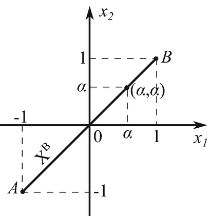

Berge equilibria

and the corresponding payoffs (Fig. 3.4) are

$$\displaystyle \begin{aligned}\varphi(\mathrm{X}^{\mathrm{B}}) = \left\{ (\alpha^2,\alpha^2) \: | \: \forall \alpha = {\mathrm{const}} \in [-1,1] \right\} = OC. \end{aligned}$$

Fig. 3.4

Corresponding payoffs

Thus, every point (α, α) of the bisecting segment AB is a Berge equilibrium in game (3.3.15). The corresponding payoffs φ(X^B) form the segment OC, as illustrated in Fig. 3.4.

Step 3. :

Then

$$\displaystyle \begin{aligned} \varphi(\mathrm{X}^B) + \psi(\mathrm{Y}_S) = \{ OC + \psi(\mathrm{Y}_S) \} = OC + \{ y_S \: | \: \forall \beta \in \left[ 0, {\pi}/{2} \right] \} = KPQL \end{aligned}$$

(see the shaded domain in Fig. 3.5).

Fig. 3.5

Set φ(X^B) + ψ(Y_S)

Step 4. :

The Slater minima of the set KPQL make up a quarter of the circumference (the bold arc PQ in Fig. 3.5), i.e.,

$$\displaystyle \begin{aligned} PQ \; = \; \left\{ 1- \cos \beta, 1- \sin \beta \: | \: \beta \in \left[ 0, {\pi}/{2} \right] \right\}. \end{aligned}$$

Each pair $((1,1), \; (1- \cos \beta , 1- \sin \beta ))$ with any $\beta \in \left [ 0, {\pi }/{2} \right ]$ is a Slater-guaranteed balanced Berge equilibrium in game (3.3.14).

Thus, the suggested algorithm dictates both players to choose $x^B_1=x^B_2=1$ (the Slater-maximal Berge equilibrium B = (1,  1) in game (3.3.14), see Fig. 3.4). In this case, the players obtain the guaranteed vector payoff $(1- \cos \beta , 1- \sin \beta )=\bar {f}^B$, i.e., for any y ∈Y the payoffs f _i((1,  1), y) cannot be simultaneously smaller than the corresponding payoffs $\bar {f}^{\mathrm {B}}_i$ (i = 1,  2). And this is the highest guarantee (in the sense of Slater) among all the guarantees $f(x^{\mathrm {B}},y_{\mathrm {S}})=(x^{\mathrm {B}}_1 - \cos \beta , x^{\mathrm {B}}_2 - \sin \beta )$ for all $\beta \in \left [ 0, {\pi }/{2} \right ]$ and any other Berge equilibria x ^B in game (3.3.15).

3.3.4 Existence in Mixed Strategies and One Remark

Not the existence theorem is the valuable thing,

but the construction carried out in the proof.

Mathematics is, as Brouwer sometimes says,

more action than theory.

—Weyl¹⁷

The existence of a Slater-guaranteed balanced Berge equilibrium in mixed strategies is established for the noncooperative N-player game under uncertainty.

Remark 3.3.1

The auxiliary noncooperative game without uncertainty (3.3.9), (3.3.8) allows us to establish the existence of a Slater-guaranteed balanced Berge equilibrium in mixed strategies in game (3.3.1) under uncertainty. Let us associate with game (3.3.1) its mixed extension

$$\displaystyle \begin{aligned} \tilde{\Gamma} = \langle \: \mathbb{N},\{ \nu_i \}_{i\in\mathbb{N}}, \{\mu\}, \{ f_i(\nu,\mu) \}_{i\in\mathbb{N}} \: \rangle, {} \end{aligned} $$

(3.3.17)

where, like in (3.3.1), $\mathbb {N} = \{ 1,\ldots ,N \}$ denotes the set of players. Assuming that the sets X_i $(i\in \mathbb {N})$ and Y are compact and the payoff functions f _i(x, y) are continuous on X ×Y, we will construct the sets {ν _i} of mixed strategies ν _i(⋅) of player i. Specifically, ν _i(⋅) is a probability measure on the Borel σ-algebra of all subsets of the compact set X_i.

The mixed uncertainties μ(⋅) represent probability measures on the compact set Y. Let {μ} denote the set of such uncertainties. The mixed strategy profiles ν(⋅) are the product measures ν(dx) = ν ₁(dx ₁)⋯ν _N(dx _N). Denote by {ν} the set of such mixed strategy profiles. In a similar fashion, define the product measures η(dxdy) = ν(dx)μ(dy); then the payoff function of player i in game (3.3.17) is the expectation

$$\displaystyle \begin{aligned}f_i(\nu,\mu) = \int\limits_{\mathrm{X}} \int\limits_{\mathrm{Y}} f_i(x,y) \mu(dy)\nu(dx) = \int\limits_{\mathrm{Y}} \int\limits_{\mathrm{X}} f_i(x,y) \nu(dx)\mu(dy). \end{aligned}$$

Recall that f  = (f ₁, …, f _N). The following concept is an analog of Definition 3.3.1 for game (3.3.17).

Definition 3.3.2

A pair $(\widetilde {\nu }^{\mathrm {B}}(\cdot ),\widetilde {f}^{\mathrm {S}}) \in \{\nu \} \times \mathbb {R}^N$ is called a Slater-guaranteed balanced Berge equilibrium (SGBBE) in the mixed extension (3.3.17) (or an SGBBE in mixed strategies in game (3.3.1) under uncertainty) if there exists a mixed uncertainty μ _S(⋅) ∈{μ} such that

$\left .(1^\circ \right ) \;$ :

the mixed strategy profile ν ^B(⋅) ∈{ν} of game (3.3.17) is a Berge equilibrium in game

$$\displaystyle \begin{aligned}\langle \: \mathbb{N},\{ \nu_i \}_{i\in\mathbb{N}}, \{ f_i(\nu,\mu_{\mathrm{S}}) \}_{i\in\mathbb{N}} \: \rangle \end{aligned}$$

(which is obtained from (3.3.17) by setting μ(⋅) = μ _S(⋅)), i.e.,

$$\displaystyle \begin{aligned} \max\limits_{\nu(\cdot) \in \{\nu\}} f_i(\nu||\nu^{\mathrm{B}}_i,\mu_{\mathrm{S}}) = f_i(\nu^{\mathrm{B}},\mu_{\mathrm{S}}) \;\;\; (i\in\mathbb{N}); {} \end{aligned} $$

(3.3.18)

(2^∘ ):

the mixed uncertainty μ _S(⋅) ∈{μ} is a Slater-minimal alternative in the N-criteria choice problem

$$\displaystyle \begin{aligned}\langle \: \{ \mu \}, \{ f_i(\nu^{\mathrm{B}},\mu) \}_{i\in\mathbb{N}} \: \rangle \end{aligned}$$

(which is obtained from (3.3.17) by setting ν(⋅) = ν ^B(⋅)), i.e.,

$$\displaystyle \begin{aligned} f(\nu^{\mathrm{B}},\mu) \nless f(\nu^{\mathrm{B}},\mu_{\mathrm{S}}) \;\;\; \forall \mu(\cdot) \in \{\mu\}; {} \end{aligned} $$

(3.3.19)

denote by {ν ^B, μ _S} the set of all product measures that satisfy (3.3.18) and (3.3.19) simultaneously;

(3^∘ ):

the pair $(\widetilde {\nu }^{\mathrm {B}}(\cdot ),\widetilde {\mu }_{\mathrm {S}}(\cdot ))$ is a Slater-maximal alternative in the N-criteria choice problem

$$\displaystyle \begin{aligned}\left \langle \: \left\{ \nu^{\mathrm{B}},\mu_{\mathrm{S}} \right \}, \{ f_i\left(\nu^{\mathrm{B}},\mu_{\mathrm{S}}\right) \}_{i\in\mathbb{N}} \: \right \rangle, \end{aligned}$$

i.e.,

$$\displaystyle \begin{aligned}\widetilde{f}^{\,\mathrm{S}} = f(\widetilde{\nu}^{\mathrm{B}},\widetilde{\mu}_{\mathrm{S}}) \nless f(\nu,\mu) \;\;\; \forall (\nu,\mu) \in \left\{\nu^{\mathrm{B}},\mu_{\mathrm{S}}\right\}. \end{aligned}$$

Theorem 3.3.2

Consider game (3.3.1) under the assumptions that the sets X_i and Y are compact and the payoff functions f _i(x, y) are continuous on X ×Y $(i\in \mathbb {N})$. Then there exists a Slater-guaranteed balanced Berge equilibrium in mixed strategies in this game.

The Advantages of Balanced Berge Equilibrium: Further Clarification

The Slater-guaranteed balanced Berge equilibrium $(\bar {x}^{\mathrm {B}},\bar {f}^{\mathrm {S}})$ introduced by Definition 3.3.1 has the following obvious pleasant features.

First, using their strategies $x^{\mathrm {B}}_i$ from a profile x ^B, the players surely obtain a guaranteed vector payoff $f^{\mathrm {B}}_i$, which is often larger (not smaller) than the vector payoff yielded by the strongly-guaranteed equilibrium; see the next section. Our aim is to increase guarantees as much as possible!

Second, this equilibrium is based on the hypothesis of “the worst-case uncertainty” for the players, i.e., on the generally accepted principle of guaranteed result under “strong uncertainty.”

Third, for calculating a Slater-guaranteed balanced Berge equilibrium, it is necessary to construct a Berge equilibrium in an auxiliary game obtained from the original game. This feature has allowed us to prove existence (see Theorem 3.3.2) under the standard assumptions of game theory.

Fourth, condition 3^∘ of Definition 3.3.1 eliminates the internal instability of the set of all Berge equilibria, since by Slater maximality it is impossible to find two balanced equilibria $(\bar {x}^{(1)},\bar {f}^{(1)})$ and $(\bar {x}^{(2)},\bar {f}^{(2)})$ such that $\bar {f}^{(1)}_i > \bar {f}^{(2)}_i$ $(i\in \mathbb {N})$, where $\bar {f}^{(j)}_i = f_i(\bar {x}^{(j)},\bar {y}^{(j)})$ (j = 1,  2).

Fifth, in the special case (3.3.10) of noncooperative games, such guaranteed equilibria are interchangeable, in the sense that a pair $(\bar {x},\bar {y})$ satisfies conditions 1^∘ and 2^∘ of Definition 3.3.1 if and only if $\bar {x} \in \mathrm {X}^{\mathrm {B}}$ and $\bar {y}\in \mathrm {Y}_{\mathrm {S}}$ (see Steps 1 and 2 in Sect. 3.3.3).

In conclusion, yet note that the concept of balanced equilibrium suffers from several drawbacks: no garden without its weeds. Their detailed description as well as some “recipes” will be given in Sects. 3.4 and 3.5.

3.4 Strongly-Guaranteed Berge Equilibrium

In the final analysis, people are equal but not always,

not everywhere and not in all respects.

—Grzegorczyk¹⁸

3.4.1 Introduction

The last thing we decide in writing a book

is what to put first.

—Pascal¹⁹

In the previous section, we have considered a solution concept for noncooperative games under uncertainty (NGUs) known as balanced Berge equilibrium, which was suggested by Zhukovskiy in [93, p. 233] back in 1994, using an appropriate modification of the concept of saddle point. The saddle point-based approach was also used for different types of equilibria in his later publications [51] and [52], the latter devoted to cooperative games. Section 3.4 presents a novel formalization for the guaranteed solutions of NGUs that relies on maximin.

3.4.2 Maximin and Its Interpretation Using Two-Level Game

Some man married a very skinny woman.

Being asked why, he said,

“I have chosen the least evil.”

—Bar Hebraeus²⁰

A hierarchical interpretation of the maximin as a two-level game is suggested.

As mentioned earlier, a single-criterion choice problem under uncertainty (SCCPU) is described by a triplet

$$\displaystyle \begin{aligned} \langle \: \mathrm{X}_1, \mathrm{Y}, f_1(x_1,y) \: \rangle, {} \end{aligned} $$

(3.4.1)

where $\mathrm {X}_1 \!\subseteq \! \mathbb {R}^{n_1}$ denotes the set of admissible alternatives of a decision maker (DM); $\mathrm {Y} \!\subseteq \!\mathbb {R}^m$ is the set of uncertain factors y; f ₁(x ₁, y) is a DM’s objective function defined on the set X₁ ×Y. He seeks to maximize this function by choosing an appropriate alternative x ₁ ∈X₁, under any realization of the uncertain factor y ∈Y.

In operations research, a solution of problem (3.4.1) is a pair $(x^{\mathrm {g}}_1,f^{\mathrm {g}}_1) \in \mathrm {X}_1 \times \mathbf {R}$ such that

$$\displaystyle \begin{aligned} f^{\mathrm{g}}_1 = \max\limits_{x_1 \in \mathrm{X}_1} \min\limits_{y\in\mathrm{Y}} f_1(x_1,y) = \min\limits_{y\in\mathrm{Y}} f_1(x^{\mathrm{g}}_1,y). {} \end{aligned} $$

(3.4.2)

It was introduced by Wald [282] in 1939. More specifically, using the alternative $x^{\mathrm {g}}_1$ the DM achieves the highest guarantee $f^{\mathrm {g}}_1 \leqslant f_1(x_1^{\mathrm {g}},y)$ for all y ∈Y (also see Remark 3.4.1).

Let us again consider problem (3.4.1), this time as the following hierarchical two-player game. Player 1 (the DM) chooses x ₁ ∈X₁, while player 2 chooses y  ∈ Y. Assume this game has a fixed sequence of moves [134, p. 79], i.e., player 1 is given priority in actions over player 2. Such a setup with the first move of player 1 describes well, e.g., an interaction of conflicting parties in a two-level hierarchical system with a single player at each level. We will also accept the hypothesis that, whenever the outcome depends on the choice of player 2 only, he always minimizes the function f ₁(x ₁, y). Player 1 is informed about this behavior.

Then player 1 takes advantage of the first move, reporting his strategy x ₁ ∈X₁ to player 2. Making the second move in this game, player 2 responds with a counter strategy y(x ₁) : X₁ →Y that minimizes the function f ₁(x ₁, y) in y for each x ₁ ∈X₁. If for each x ₁ this minimum is achieved at a unique point y(x ₁), then the best (guaranteed) result of player 1 gives

$$\displaystyle \begin{aligned} f^{\mathrm{g}}_1 &= \max\limits_{x_1\in\mathrm{X}_1} \min\limits_{y\in\mathrm{Y}} f_1(x_1,y) = \max\limits_{x_1\in\mathrm{X}_1} f_1(x_1,y(x_1))\\ &= f_1\left(x^{\mathrm{g}}_1,y\left(x^{\mathrm{g}}_1\right)\right) = \min\limits_{y\in\mathrm{Y}} f_1\left(x^{\mathrm{g}}_1,y\right). \end{aligned} $$

The sequence of moves of the DM and of player 2 is illustrated in Fig. 3.6.

Fig. 3.6

Hierarchy in maximin setup

As a result, the DM prefers the maximin strategy $x_1^{\mathrm {g}}$, which yields the best guaranteed payoff

$$\displaystyle \begin{aligned}f_1^{\mathrm{g}} \leqslant f(x_1^{\mathrm{g}},y) \;\;\;\; \forall y \in \mathrm{Y}. \end{aligned}$$

Note that, for all x ₁ ∈X₁, this payoff exceeds all other guaranteed payoffs

$$\displaystyle \begin{aligned}f_1(x_1,y(x_1)) = \min\limits_{y\in \mathrm{Y}} f_1(x_1,y) \leqslant f_1(x_1,y) \;\;\; \forall \: x_1 \in \mathrm{X}_1. \end{aligned}$$

Remark 3.4.1

The design operation y(x ₁) : X₁ →Y corresponds to the calculation of the inner minimum

$$\displaystyle \begin{aligned}f_1(x_1,y(x_1)) = \min\limits_{y\in \mathrm{Y}} f_1(x_1,y) \;\;\; \forall x_1 \in \mathrm{X}_1 \end{aligned}$$

in the maximin formula (3.4.2). On the other hand, the definition of $x^{\mathrm {g}}_1$ using

$$\displaystyle \begin{aligned}f_1(x^{\mathrm{g}},y\left(x_1^{\mathrm{g}}\right) = \max\limits_{x_1\in \mathrm{X}_1} f_1(x_1,y(x_1)) \end{aligned}$$

matches the outer maximum in (3.4.2). Actually, the application of these operations (inner minimum and outer maximum) to the NGUs underlies the concepts of guaranteed equilibria formalized below.

3.4.3 Drawback of Balanced Equilibrium as Solution of Noncooperative Game Under Uncertainty

Nobody can be perfect unless he admits his faults,

but if he has faults how can he be perfect?

—Peter²¹

A major drawback of the balanced equilibrium is identified and two alternative types of guaranteed equilibria for the NGU are suggested.

In Sect. 3.3, we have considered the NGU

$$\displaystyle \begin{aligned} \langle \: \mathbb{N}, \{\mathrm{X}_i\}_{i \in \mathbb{N}}, \mathrm{Y}, \{f_i(x,y)\}_{i\in\mathbb{N}} \: \rangle, {} \end{aligned} $$

(3.4.3)

where $\mathbb {N} = \{ 1, \ldots , N \}$ is the set of players; $\mathrm {X}_i \subseteq \mathbb {R}^{n_i}$ is the set of pure strategies x _i of player i; $\mathrm {X} = \prod \limits _{i\in \mathbb {N}} \mathrm {X}_i$ is the set of all pure strategy profiles x = (x ₁, …, x _N); $\mathrm {Y} \subseteq \mathbb {R}^m$ is the set of pure uncertainties y; finally, f _i(x, y) is the payoff function of player i, defined on X ×Y. Using an appropriate modification of the saddle point, balanced equilibrium has been formalized by Definition 3.3.1 as a first concept of guaranteed solution of game (3.4.3).

At the end of Sect. 3.3.3, we have also pointed to a negative feature of this concept, which stems from the following circumstance. In accordance with condition 1^∘ of Definition 3.3.1, a strategy profile $\bar {x}^{\mathrm {B}} \in \mathrm {X}$ is a Berge equilibrium if

$$\displaystyle \begin{aligned} \max\limits_{x \in \mathrm{X}} f_i\left(\bar{x}||x^{\mathrm{B}}_i,y_S\right) = f_i\left(\bar{x}^{\mathrm{B}},y_{\mathrm{S}}\right), {} \end{aligned} $$

(3.4.4)

where the uncertain factor y _S has a frozen value. However, even the problem statement postulates that the uncertain factor y may take arbitrary values from Y, and orientation towards a specific value y _S is quite delusive (note that equalities (3.4.4) do not necessarily hold for other y ≠ y _S). If some value y ∈Y, y ≠ y _S, is realized in game (3.4.3), then generally the strategy profile x ^B fails to be a Berge equilibrium; moreover, x ^B yields the vector guarantee $\bar {f}^{\mathrm {S}}=f(\bar {x}^{\mathrm {B}},\bar {y}_{\mathrm {S}})$ only if all players adhere to their strategies from the profile x ^B (without any deviations from x ^B allowed). Nevertheless, a series of considerable advantages in favor of Slater-guaranteed balanced Berge equilibrium have been outlined in Sect. 3.3; in some cases (e.g., for payoff functions with separate components in x and y), this equilibrium becomes rather useful in applications. The negative feature can be eliminated using a strongly-guaranteed equilibrium or Slater-guaranteed equilibrium as the solution concepts of the NGUs; see Sects. 3.4.4 and 3.4.5 for a detailed description.

3.4.4 Formalization

…nothing whatsoever takes place in the universe in which

some relation of maximum and minimum does not appear.

—L. Euler²²

A guaranteed solution of a noncooperative game under uncertainty is proposed, which (in our view) is the most obvious concept among the ones analyzed in Sect. 3.3 and below.

Consider the noncooperative game under uncertainty with a possible information discrimination of players:

$$\displaystyle \begin{aligned} \Gamma = \langle \mathbb{N} ,\{ \mathrm{X}_i\}_{i \in \mathbb{N} }, \mathrm{Y^X}, \{f_i(x,y)\}_{i \in \mathbb{N} } \rangle. {} \end{aligned} $$

(3.4.5)

In this game, $\mathbb {N} =\{1,2,\ldots ,N\}$ denotes the set of players; $\mathrm {X}_i \subseteq \mathbb {R}^{n_i}$ is the set of pure strategies x _i of player i, and a vector $x=(x_1,\ldots ,x_N) \in \mathrm {X} = \prod \mathrm {X}_i$ forms a pure strategy profile in the game Γ; $\mathrm {Y} \subseteq \mathbb {R}^m$ is the set of uncertain factors y; Y^X is the set of functions y(x) defined on X and taking values from Y; these m-dimensional vector functions y(x) will be called “aware” uncertainties in game (3.4.5); finally, f _i(x, y) = f _i(x, y(x)) gives the payoff function of player i $( i \in \mathbb {N} )$.

This game runs as follows. The players simultaneously choose their individual strategies x _i ∈X_i $( i \in \mathbb {N} )$ without building any coalitions. As a result, we have a strategy profile in the game Γ, i.e., an ordered collection of strategies x = (x ₁, …, x _N) ∈X = X₁ ×⋯ ×X_N. Let us accept the hypotheses about the information discrimination of players and the additional awareness of uncertainty. That is, by analogy with the hierarchical games considered in Sect. 3.4.2, the first move belongs to the players: they choose and then report their strategies x _i ∈X_i to a DM, who is “in charge of” uncertainty design. The second move is given to the DM—he generates N uncertain factors in the form of continuous m-dimensional vector functions y ⁽ⁱ⁾(x) $(i\in \mathbb {N})$ defined on the set X and then reports them to all N players. Assume the worst-case uncertainties, which spoil the individual payoff of each player as much as possible. Using this information, the players choose a strategy profile x ^B  ∈ X yielding a “good” payoff f _i(x ^B, y(x ^B)) (e.g., a Berge equilibrium) for each player i $(i \!\in \!\mathbb {N} )$. The Slater-maximal profile $\bar {x}^{\mathrm {B}}$ is selected from the set of all good profiles. The point is that the set of Berge equilibria {x ^B} has internal instability (see Example 3.3.1), i.e., there may exist two profiles x ^(j) ∈{x ^B} (j = 1,  2) such that f _i[x ⁽¹⁾] > f _i[x ⁽²⁾] $(i\in \mathbb {N})$. This drawback is eliminated by using the Slater maximality of $\bar {x}^B$. The hierarchical decision-making procedure of NGU (3.4.5) is illustrated in Fig. 3.7.

Fig. 3.7

Decision-making in the NGU (3.4.5)

Note that sometimes it is necessary to adopt mixed strategies instead of the pure ones in order to prove the existence of these good solutions—the strategy profiles in game (3.4.5). In fact, this approach will be used in the current and forthcoming sections.

Recall that the guaranteed solution $(x^{\mathrm {g}}_1,f^{\mathrm {g}}_1)$ of a single-criterion choice problem

$$\displaystyle \begin{aligned}\langle \mathrm{X}_1, \mathrm{Y}, f_1(x_1,y) \rangle \end{aligned}$$

is described by the chain of equalities

$$\displaystyle \begin{aligned}f^{\mathrm{g}}_1 \; = \; \max\limits_{x_1\in\mathrm{X}_1} \min\limits_{y\in\mathrm{Y}} f_1(x_1,y) \; = \; \min\limits_{y\in\mathrm{Y}} f_1\left(x^{\mathrm{g}}_1,y\right). \end{aligned}$$

First, we have to calculate the inner minimum

$$\displaystyle \begin{aligned}y(x_1) = \arg\min\limits_{y\in\mathrm{Y}} f_1(x_1,y), \end{aligned}$$

and then outer maximum

$$\displaystyle \begin{aligned}x^{\mathrm{g}}_1 \; = \; \arg\max\limits_{x_1\in\mathrm{X}_1} f_1(x_1,y(x_1)), \;\;\; f^{\mathrm{g}}_1 \; = \; f_1\left(x^{\mathrm{g}}_1,y\left(x^{\mathrm{g}}_1\right)\right). \end{aligned}$$

Let us clarify the optimal meaning of these concepts.

First, it follows from $f^{\mathrm {g}}_1 = \min \limits _{y\in \mathrm {Y}} f_1(x^{\mathrm {g}}_1,y)$ that

$$\displaystyle \begin{aligned}f^{\mathrm{g}}_1 \; \leqslant \; f_1\left(x^{\mathrm{g}}_1,y\right) \;\;\; \forall y \in \mathrm{Y}, \end{aligned}$$

i.e., with the strategy $x^{\mathrm {g}}_1$ the DM obtains the guaranteed outcome $f^{\mathrm {g}}_1$ under any realization of the uncertain factor y ∈Y.

Second, since $f_1[x_1] = \min \limits _{y\in \mathrm {Y}} f_1(x_1,y) = f_1(x_1,y(x_1))$, with any strategy x ₁ ∈X₁ the DM obtains a guaranteed outcome

$$\displaystyle \begin{aligned}f_1[x_1] \; \leqslant \; f_1(x_1,y) \;\;\; \forall y \in \mathrm{Y}, \end{aligned}$$

and the guarantee $f^{\mathrm {g}}_1$ is highest because

$$\displaystyle \begin{aligned}f^{\mathrm{g}}_1 \; = \; f_1\left(x^{\mathrm{g}}_1,y\left(x^{\mathrm{g}}_1\right)\right) \; \geqslant \; f_1[x_1] \; = \; f_1(x_1,y(x_1)) \;\;\; \forall x_1 \in \mathrm{X}_1. \end{aligned}$$

The concept of strongly-guaranteed solution of game (3.4.5) that is introduced below relies on a modification of these two properties of maximin. The modification itself consists in replacing the inner minimum by N scalar minima, i.e.,

$$\displaystyle \begin{aligned}\min\limits_{y\in\mathrm{Y}} f_i(x,y) = f_i(x,y^{(i)}(x)) = f_i[x] \;\; \forall x \in \mathrm{X} \;\; ( i \in \mathbb{N} ), \end{aligned}$$

and also in replacing the outer maximum by the concept of Berge equilibrium, i.e.,

$$\displaystyle \begin{aligned}\max\limits_{x\in\mathrm{X}} f_i\left[x||x^{\mathrm{B}}_i\right] = f_i\left[x^{\mathrm{B}}\right] \;\; ( i \in \mathbb{N}), \end{aligned}$$

where $[x||x^{\mathrm {B}}_i]=[x_1,\ldots ,x_{i-1},x^{\mathrm {B}}_i,x_{i+1},\ldots ,x_N]$.

We will formalize the concept of Slater-strongly-guaranteed Berge equilibrium in three steps as follows.

Step 1.:

Associate with each strategy profile x  ∈ X and each player $i \!\in \! \mathbb {N}$ a unique continuous vector function y ⁽ⁱ⁾(x) on X such that

$$\displaystyle \begin{aligned} f_i\left(x,y^{(i)}(x)\right) = \min\limits_{y\in\mathrm{Y}} f_i(x,y) = f_i[x] \;\;\; (i \in \mathbb{N}). {} \end{aligned} $$

(3.4.6)

Step 2.:

Associate with game (3.4.5) the noncooperative N-player game (without uncertainty)

$$\displaystyle \begin{aligned} \langle \mathbb{N} ,\{ \mathrm{X}_i\}_{i \in \mathbb{N} }, \{f_i[x]\}_{i \in \mathbb{N} } \rangle, {} \end{aligned} $$

(3.4.7)

further referred to as the game of guarantees. For this game, find a Berge equilibrium x ^B ∈X from the equalities

$$\displaystyle \begin{aligned} \max\limits_{x\in\mathrm{X}} f_i \left[x||\:x^{\mathrm{B}}_i\right] = f_i\left[x^{\mathrm{B}}\right] \;\;\; (i \in \mathbb{N}). {} \end{aligned} $$

(3.4.8)

Step 3.:

From the set of all Berge equilibria {x ^B}, choose the maximal one $\bar {x}^{\mathrm {B}}$ in the vector sense, e.g., find a Slater-maximal alternative $\bar {x}^{\mathrm {B}}$ in the N-criteria choice problem

$$\displaystyle \begin{aligned}\left \langle \: \left\{x^{\mathrm{B}}\right\}, \{f_i[x]\}_{i \in \mathbb{N} } \: \right \rangle. \end{aligned}$$

In the case of Slater maximum, it suffices to calculate $\bar {x}^{\mathrm {B}}$ using the condition

$$\displaystyle \begin{aligned}\max\limits_{x\in \{x^B\}} \sum_{i \in \mathbb{N}} \alpha_i f_i[x] \; = \; \sum_{i \in \mathbb{N}} \alpha_i \bar{f}_i\left[\bar{x}^{\mathrm{B}}\right], \end{aligned}$$

where all the constants $\alpha _i \geqslant 0 \: (i \in \mathbb {N}) \: \wedge \: \sum \limits _{i \in \mathbb {N}}\alpha _i > 0$, see [152, pp. 68–69].

Finally, construct the N-dimensional vector

$$\displaystyle \begin{aligned}\bar{f}\left[\bar{x}^{\mathrm{B}}\right] = \left( \bar{f}_1\left[\bar{x}^{\mathrm{B}}\right],\ldots,\bar{f}_N\left[\bar{x}^{\mathrm{B}}\right] \right). \end{aligned}$$

The resulting pair $(\bar {x}^{\mathrm {B}},\bar {f}[\bar {x}^{\mathrm {B}}]) \in \mathrm {X}\times \mathbb {R}^N$, where f = (f ₁, …, f _N), will be called the Slater-strongly-guaranteed Berge equilibrium in game (3.4.5); in addition, $\bar {x}^{\mathrm {B}}$ is the strongly-guaranteeing strategy profile in game (3.4.5) while $\bar {f}_i[\bar {x}^{\mathrm {B}}]$ is the strongly-guaranteed payoff of player $i \in \mathbb {N}$.

The game-theoretic meaning of the suggested solution consists in the following. If the players have chosen the strategies x _i ∈X_i $(i \in \mathbb {N})$, thereby forming the profile x = (x ₁, …, x _N), then each player i obtains a payoff f _i(x, y) not smaller than f _i[x] (3.4.6) under any realization of the uncertain factor y  ∈ Y. (This fact follows from the last equality of (3.4.6), written in the form $f_i[x] \; \leqslant \; f_i(x,y) \;\;\; \forall y \in \mathrm {Y})$. In other words, the value f _i[x] is the guarantee for player i under the players’ strategies from the profile x ∈X and any realization of the uncertain factor y ∈Y, regardless of their choice.

Next, in accordance with Step 2 (see the definition), instead of the noncooperative game under uncertainty (3.4.5) one has to consider the game of guarantees (3.4.7), (3.4.6) without uncertainty. In this game, the payoff functions of the players are their guarantees f _i[x] $(i \in \mathbb {N})$, while the Berge equilibrium is defined by the same principle, now applied to the new payoff functions—the guarantees f _i[x] $(i \in \mathbb {N})$ of the original payoff functions f _i(x, y).

The strongly-guaranteed equilibrium is stable in the sense that, if the players choose their strategies from the profile $x^{\mathrm {B}}=(x^{\mathrm {B}}_1,\ldots ,x^{\mathrm {B}}_N)$, then

First, under any realization of the uncertain factor y ∈Y the conflicting parties obtain guaranteed payoffs $f_i(x^{\mathrm {B}},y) \geqslant f_i[x^{\mathrm {B}}]=f^{\mathrm {B}}_i$ $(i \in \mathbb {N})$ that are not smaller than their guarantees;

Second, any deviation, e.g., of player 1 from the strategy $x^{\mathrm {B}}_1$ (i.e., the choice of another strategy $\tilde {x}_1 \!\in \!\mathrm {X}$ such that $\tilde {x}_1 \!\neq \! x^{\mathrm {B}}_1$) gives, e.g., to player 2 a payoff $f_2(x^{\mathrm {B}}||\tilde {x}_1,y)$ with a guarantee $f_2[x^{\mathrm {B}}||\tilde {x}_1]$ not higher than the guarantee f ₂[x ^B] in the equilibrium x ^B (the noncooperative game under uncertainty (3.4.5) is assessed using the game of guarantees (3.4.7)).

3.4.5 Existence in Mixed Strategies

The existence of a strongly-guaranteed Berge equilibrium in mixed strategies is established for the noncooperative two-player game under uncertainty with continuous payoff functions that are strictly convex in the uncertain factors, and also with compact sets of strategies and uncertain factors.

To simplify notation, our analysis below will be confined to game (3.4.5) with two players, i.e., $\mathbb {N} = \{ 1,2 \}$.

Let the sets X_i $(i\!=\!1,2)$ be convex and compact and consider the Borel σ-algebra of all subsets of the set X_i (the details can be found in Remark 3.3.1); as an extension of the set of (pure) strategies x _i  ∈ X_i of player i, consider his mixed strategies μ _i(⋅)—probability measures on the compact set X_i, i.e., on the Borel σ-algebra of the set X_i. Denote by {μ _i} (i = 1,  2) the set of mixed strategies of player i. Note that a measure of the form $\delta (x_i - x_i^{*})(dx_i)$, where δ(⋅) is the Dirac function, is also a mixed strategy of player i. The product measures μ(dx ₁, dx ₂) introduced by the definitions in [122, p. 271] with the notations [108, p. 284],

$$\displaystyle \begin{aligned}\mu(dx_1,dx_2) \; = \; \mu_1(dx_1)\mu_2(dx_2), \end{aligned}$$

are probability measures on the product X = X₁ ×X₂ of the compact sets X₁ and X₂. To construct the product measure μ(dx ₁, dx ₂), as the σ-algebra of all subsets X₁ ×X₂ one takes the smallest Borel σ-algebra containing all the products Q ₁ × Q ₂, where Q _i is an element of the Borel σ-algebra of the compact set X_i (i = 1,  2).

If the payoff functions f _i[x ₁, x ₂] are continuous on X₁ ×X₂, we define the following integrals in terms of expectation:

$$\displaystyle \begin{aligned}f_i[\mu_1,x_2] = \int\limits_{\mathrm{X}_1} f_i[x_1,x_2]\mu_1(dx_1), \;\;\;\; f_i[x_1,\mu_2] = \int\limits_{\mathrm{X}_2} f_i[x_1,x_2]\mu_2(dx_2). \end{aligned}$$

Since the functions f _i[x ₁, x ₂] are continuous on X₁ ×X₂, the integrals f _i[μ ₁, x ₂] and f _i[x ₁, μ ₂] are continuous functionals on X₂ and X₁, respectively; see [24, p. 113]. Then there exist the double integrals

$$\displaystyle \begin{aligned} & f_i[\mu_1,\mu_2] = \int\limits_{\mathrm{X}_2} f_i[\mu_1,x_2]\mu_2(dx_2) = \int\limits_{\mathrm{X}_2} \int\limits_{\mathrm{X}_1} f_i[x_1,x_2]\mu_1(dx_1)\mu_2(dx_2),\\ & \quad \int\limits_{\mathrm{X}_1} f_i[x_1,\mu_2]\mu_1(dx_1) = \int\limits_{\mathrm{X}_1} \int\limits_{\mathrm{X}_2} f_i[x_1,x_2]\mu_2(dx_2)\mu_1(dx_1), \end{aligned} $$

which take the same value by Fubini’s theorem.

Now let us pass to the mixed extension of game (3.4.7) with $\mathbb {N} =\{ 1,2 \}$, i.e., to the noncooperative game

$$\displaystyle \begin{aligned}\tilde{\Gamma}_2 = \langle \{ 1,2 \},\{ \mu_i\}_{i =1,2}, \{f_i[\mu_1,\mu_2]\}_{i=1,2} \rangle, \end{aligned}$$

where {μ _i} is the set of mixed strategies μ _i(⋅) of player i, which are probability measures on the compact set X_i; the expectation

$$\displaystyle \begin{aligned}f_i[\mu_1,\mu_2] \; = \int\limits_{\mathrm{X}_1 \times \mathrm{X}_2} f_i[x_1,x_2]\mu_1(dx_1)\mu_2(dx_2) \end{aligned}$$

gives the mixed extension of the payoff function f _i[x ₁, x ₂] (i = 1,  2).

A pair of mixed strategies $(\mu ^{\mathrm {B}}_1(\cdot ),\mu ^{\mathrm {B}}_2(\cdot )) \in \{ \mu _1\} \times \{ \mu _2\}$ is called a Berge equilibrium in game $\tilde {\Gamma }_2$ if

$$\displaystyle \begin{aligned} \begin{array}{c} f_1[\mu^{\mathrm{B}}_1,\mu_2] \leqslant f_1[\mu^{\mathrm{B}}_1,\mu^{\mathrm{B}}_2] \;\;\;\; \forall \mu_2(\cdot) \in \{ \mu_2 \}, \\ f_2[\mu_1,\mu^{\mathrm{B}}_2] \leqslant f_2[\mu^{\mathrm{B}}_1,\mu^{\mathrm{B}}_2] \;\;\;\; \forall \mu_1(\cdot) \in \{ \mu_1 \}. \end{array} {} \end{aligned} $$

(3.4.9)

Interestingly, the set of all payoffs f[μ ^B] = (f ₁[μ ^B], f ₂[μ ^B]) on the set of all Berge equilibria $\{ \mu ^{\mathrm {B}}(\cdot ) = \mu _1^{\mathrm {B}}(\cdot )\mu _2^{\mathrm {B}}(\cdot ) \}$ is compact in $\mathbb {R}^{2}$ (this follows from Proposition 3.4.1 below).

In accordance with [22, pp. 117–119], if in the game $\tilde {\Gamma }_2$ the payoff functions f _i[x ₁, x ₂] are continuous on X₁ ×X₂ and the sets X_i are compact (i = 1,  2), then the game $\tilde {\Gamma }_2$ possesses a Berge equilibrium

$$\displaystyle \begin{aligned}\mu^{\mathrm{B}}(\cdot) = \left(\mu^{\mathrm{B}}_1(\cdot),\mu^{\mathrm{B}}_2(\cdot)\right) \in\{ \mu_1\} \times \{ \mu_2\}.\end{aligned}$$

Sometimes, this profile is called a mixed strategy Berge equilibrium in game (3.4.7) with $\mathbb {N} = \{ 1,2 \}$.

Proposition 3.4.1

Assume that in game (3.4.7) with $\mathbb {N} \!=\! \{ 1,2 \}$ the sets X_i (i = 1,  2) are convex and compact and the payoff functions f _i[x ₁, x ₂] are continuous on X₁ ×X₂. Then the set $\mathcal {F}^{\mathrm {B}} = \{ f_1[\mu ^{\mathrm {B}}],f_2[\mu ^{\mathrm {B}}]\}$ of all Berge equilibrium payoffs in the game $\tilde {\Gamma }_2$ is a non-empty and compact set, i.e., a closed bounded subset of $\mathbb {R}^{2}$.

Proof

In view of the well-known properties of probability measures [41, p. 288]; [122, p. 254], the set of all possible product measures μ(dx ₁, dx ₂)  =  μ ₁(dx ₁)μ ₂(dx ₂) is weakly closed and weakly compact [122, pp. 212, 254]; [180, pp. 48, 49]. Hence, from each sequence

$$\displaystyle \begin{aligned}\left \{ \mu^{(k)}(dx)\!= \!\mu^{(k)}_1(dx_1)\mu^{(k)}_2(dx_2) \right \} \;\; (k=1,2,\ldots)\end{aligned}$$

one can extract a subsequence

$$\displaystyle \begin{aligned}\left \{ \mu^{(k_j)}(dx) = \mu^{(k_j)}_1(dx_1)\mu^{(k_j)}_2(dx_2) \right \} \;\; (j=1,2,\ldots)\end{aligned}$$

that weakly converges [122, p. 212, 254]; [105, p. 199] to a function μ(⋅)  ∈ ∈ {μ}, i.e., for any choice of a continuous scalar function φ[x ₁, x ₂] defined on X, it holds that

$$\displaystyle \begin{aligned}\lim_{j \rightarrow \infty} \int\limits_{\mathrm{X}} \varphi [x_1,x_2] \mu^{(k_j)}(dx) = \int\limits_{\mathrm{X}} \varphi [x_1,x_2] \mu(dx). \end{aligned}$$

Denote by ${\mathfrak M}^B$ the set of all Berge equilibria $\mu ^{\mathrm {B}}(dx)=\mu _1^{\mathrm {B}}(dx_1)\mu _2^{\mathrm {B}}(dx_2)$ described by formulas (3.4.9). Then ${\mathfrak M}^B \neq \varnothing$, as shown in [22, pp. 117–119]. Now, take an arbitrary infinite sequence of such equilibria $\mu ^{(k)}(\cdot ) \in {\mathfrak M}^B$ (k = 1,  2, …). Owing to the weak compactness of the set of probability measures, there exist a subsequence of measures $\mu ^{(k_j)}(\cdot ) \in {\mathfrak M}^B$ (j = 1,  2, …) and a probability measure μ ^(o)(⋅) ∈{μ} such that, for a continuous function f _i[x] = f _i[x ₁, x ₂] on X,

$$\displaystyle \begin{aligned}\lim_{j \rightarrow \infty} f_i\left[\mu^{(k_j)}\right] = \lim_{j \rightarrow \infty} \int\limits_{\mathrm{X}} f_i [x] \mu^{(k_j)}(dx) = \int\limits_{\mathrm{X}} f_i [x] \mu^{(\mathrm{o})}(dx) = f_i \left[\mu^{(\mathrm{o})}\right]. \end{aligned}$$

Let us show that the limiting measure $\mu ^{(\mathrm {o})}(\cdot ) = \mu ^{(\mathrm {o})}_1(\cdot ) \mu ^{(\mathrm {o})}_2(\cdot )$ is also a Berge equilibrium, i.e.,

$$\displaystyle \begin{aligned}\begin{array}{c} f_1[\mu^{(o)}_1,\mu_2] \leqslant f_1[\mu^{(\mathrm{o})}] \;\;\;\; \forall \mu_2(\cdot) \in \{ \mu_2 \}, \\ f_2[\mu_1,\mu^{(o)}_2] \leqslant f_2[\mu^{(\mathrm{o})}] \;\;\;\; \forall \mu_1(\cdot) \in \{ \mu_1 \}. \\ \end{array} \end{aligned}$$

Assume on the contrary that there exists a measure $\bar {\mu }_1(\cdot ) \in \{ \mu _1 \}$ or a measure $\bar {\mu }_2(\cdot ) \in \{ \mu _2 \}$ such that

$$\displaystyle \begin{aligned}f_1\left[\mu^{(\mathrm{o})}_1,\bar{\mu}_2\right] > f_1\left[\mu^{(\mathrm{o})}\right] \;\; \vee \;\; f_2[\bar{\mu}_1,\mu^{(\mathrm{o})}_2] > f_2\left[\mu^{(\mathrm{o})}\right]. \end{aligned}$$

For example, let

$$\displaystyle \begin{aligned}f_1\left[\mu^{(\mathrm{o})}_1,\bar{\mu}_2\right] > f_1\left[\mu^{(\mathrm{o})}\right], \end{aligned}$$

which is equivalently written as

$$\displaystyle \begin{aligned}\int\limits_{\mathrm{X}} f_1 [x] \mu^{(\mathrm{o})}_1(dx_1) \bar{\mu}_2(dx_2) > \int\limits_{\mathrm{X}} f_1 [x] \mu^{(\mathrm{o})}(dx). \end{aligned}$$

Then, for sufficiently large j,

$$\displaystyle \begin{aligned}\int\limits_{\mathrm{X}} f_1 [x] \mu^{(k_j)}_1(dx_1) \bar{\mu}_2(dx_2) > \int\limits_{\mathrm{X}} f_1 [x] \mu^{(k_j)}(dx), \end{aligned}$$

which contradicts the inclusion $\mu ^{(k_j)}(\cdot ) \in {\mathfrak M}^B$, i.e., the Berge equilibrium condition of each mixed strategy profile $\mu ^{(k_j)}(\cdot ) \in {\mathfrak M}^B$ in the game $\widetilde {\Gamma }_2$. Hence, the set $\mathcal {F}^{\mathrm {B}} =$ $= \{ f_1[\mu ^B],f_2[\mu ^B] \: | \: \forall \mu ^B(\cdot ) \in {\mathfrak M}^B \}$ is compact in $\mathbb {R}^{2}. \;\;\; \hfill \blacksquare$

Our next task is to construct a strongly-guaranteed Berge equilibrium in mixed strategies for this game using Steps 1–3 above.

Consider game (3.4.5) with N = 2 in which the sets X_i (i = 1,  2) and Y are compact and the payoff functions f _i(x ₁, x ₂, y) (i = 1,  2) are continuous on X₁ ×X₂ ×Y.

A quadruple $(\bar {\mu }^{\mathrm {B}}_1(\cdot ),\bar {\mu }^{\mathrm {B}}_2(\cdot ),\bar {f}^{\mathrm {B}}_1,\bar {f}^{\mathrm {B}}_2) \in \{\mu _1\} \times \{\mu _2\} \times \mathbb {R}^{2}$ is called a strongly-guaranteed Berge equilibrium in mixed strategies in game (3.4.5) with N = 2 if for each i there exists a unique continuous m-dimensional vector functions y ⁽ⁱ⁾(x) : X₁ ×X₂ →Y (i = 1,  2) such that inequalities (3.4.9) hold for the function f _i[μ ₁, μ ₂] (i = 1,  2) and the product measure $\bar {\mu }^{\mathrm {B}}(\cdot )=\bar {\mu }^{\mathrm {B}}_1(\cdot )\bar {\mu }^{\mathrm {B}}_2(\cdot )$ yields a Slater-maximal alternative in the bicriteria choice problem

$$\displaystyle \begin{aligned}\langle \{ \mu^{\mathrm{B}}\}, \{ f_i[\mu] \}_{i =1,2 } \rangle. \end{aligned}$$

Here $f_i[\mu ]\!=\!f_i[\mu _1,\mu _2] \!=\! \int \limits _{\mathrm {X}} f_i[x]\mu _1(dx_1)\mu _2(dx_2)$, $f_i[x] \!=\! f_i(x,y^{(i)}(x)) = \min \nolimits _{y\in \mathrm {Y}}f_i(x,y)$, $\bar {\mu }^{\mathrm {B}}_i(\cdot ) \in \{ \mu _i \}$ indicates the mixed strategy of player i, and $\bar {f}^{\mathrm {B}}_i = \bar {f}_i[\mu ^{\mathrm {B}}_1,\mu ^{\mathrm {B}}_2]$ (i = 1,  2) is his guaranteed payoff.

Theorem 3.4.1

Consider the noncooperative two-player game under uncertainty

$$\displaystyle \begin{aligned}\Gamma_2 = \langle \{ 1,2 \},\{ \mathrm{X}_i\}_{i =1,2 }, \mathrm{Y^X}, \{f_i(x_1,x_2,y)\}_{i =1,2 } \rangle \end{aligned}$$

under the assumptions that

$\left (1^0 \right )$ :

the set $\mathrm {X}_i \subset \mathbb {R}^{n_i}$ of all pure strategies x _i of player i is convex and compact (i = 1,  2) and the set $\mathrm {Y} \subset \mathbb {R}^{m}$ of uncertain factors y is convex and compact;

$\left (2^0 \right )$ :

the payoff function f _i(x, y) of player i (i = 1,  2) is continuous on X₁ ×X₂ ×Y and strictly convex in y ∈Y for each (x ₁, x ₂) ∈X₁ ×X₂.

Then there exists a strongly-guaranteed Berge equilibrium in mixed strategies in this game.

Proof

Using the compactness of the sets X_i (i = 1,  2) and Y, the concavity of Y and also the continuity of the payoff functions f _i(x ₁, x ₂, y) on X₁ ×X₂ ×Y and their strict convexity in y ∈Y for each x = (x ₁, x ₂) ∈X₁  × X₂, we conclude (see [14, p. 54]) that there exist two continuous m-dimensional vector functions y ⁽ⁱ⁾(x ₁, x ₂) defined on X₁  × X₂ such that

$$\displaystyle \begin{aligned}\min\limits_{y\in\mathrm{Y}} f_i(x_1,x_2,y) = f_i\left(x_1,x_2,y^{(i)}(x_1,x_2)\right) = f_i[x_1,x_2] \;\;\; (i=1,2) \end{aligned}$$

for any (x ₁, x ₂) ∈X₁ ×X₂. The functions

$$\displaystyle \begin{aligned}f_i\left(x_1,x_2,y^{(i)}(x_1,x_2)\right) = f_i[x_1,x_2] \;\;\; (i=1,2) \end{aligned}$$

are continuous on X₁ ×X₂ as superpositions of the continuous functions f _i(x ₁, x ₂, y) and y = y ⁽ⁱ⁾(x ₁, x ₂).

Now, design a noncooperative two-player game—the game of guarantees

$$\displaystyle \begin{aligned} \langle \{ 1,2 \},\{ \mathrm{X}_i\}_{i =1,2 }, \{f_i[x_1,x_2]\}_{i =1,2 } \rangle. {} \end{aligned} $$

(3.4.10)

As established earlier, in this game the payoff function f _i[x ₁, x ₂] of player i $(i\!=\!1,2)$ is continuous on the product X₁ ×X₂ of compact sets. Consequently, by [22, pp. 117–119], there exists a mixed strategy Berge equilibrium $(\mu ^{\mathrm {B}}_1(\cdot ),\mu ^{\mathrm {B}}_2(\cdot )) \!\in \{ \mu _1 \} \times \{ \mu _2 \}$, which satisfies inequalities (3.4.9). Then construct the pair

$$\displaystyle \begin{aligned}f_i\left[\mu^{\mathrm{B}}\right] = f_i\left[\mu^{\mathrm{B}}_1,\mu^{\mathrm{B}}_2\right] = \int\limits_{\mathrm{X}_1 \times \mathrm{X}_2} f_i[x_1,x_2]\mu^{\mathrm{B}}_1(dx_1)\mu^{\mathrm{B}}_2(dx_2) \;\;\; (i=1,2), \end{aligned}$$

in which the set $\{ f_i[\mu ^{\mathrm {B}}] \!\!=\!\! f_i[\mu ^{\mathrm {B}}_1,\mu ^{\mathrm {B}}_2] \}$ is compact in $\mathbb {R}^2$ (see Proposition 3.4.1); ${\mathfrak M}^{\mathrm {B}}$ forms the set of all Berge equilibria $\mu ^{\mathrm {B}}(\cdot ) \!=\! \mu ^{\mathrm {B}}_1(\cdot ) \mu ^{\mathrm {B}}_2(\cdot )$ (each of them satisfies inequalities (3.4.9)). This compact set is nonempty [22, pp. 117–119]; denote it by $\mathcal {F}^B$. Consider a continuous function $\sum _{i=1}^2 \alpha _i f_i$, where α _i  =  const > 0 and $i \!\in \! \mathbb {N} \!=\!\{ 1,2 \}$, on the compact set $\mathcal {F}^B$. By the Weierstrass theorem, there exists a vector $\bar {f}^{\mathrm {B}} \!=\! (\bar {f}^{\mathrm {B}}_1,\bar {f}^{\mathrm {B}}_2) \!\in \! \mathcal {F}^{\mathrm {B}}$ such that

$$\displaystyle \begin{aligned}\max\limits_{f \in \mathcal{F}^B} \sum_{i=1}^2 \alpha_i f_i = \sum_{i=1}^2 \alpha_i \bar{f}^{\mathrm{B}}_i. \end{aligned}$$

Finally, find the product measure $\bar {\mu }^{\mathrm {B}}(\cdot ) = \bar {\mu }^{\mathrm {B}}_1(\cdot ) \bar {\mu }^{\mathrm {B}}_2(\cdot )$ from the equalities $\bar {f}^{\mathrm {B}}_i = f_i[\bar {\mu }^{\mathrm {B}}]$ (i = 1,  2).

By definition, the resulting triplet $(\bar {\mu }^{\mathrm {B}}(\cdot ),\bar {f}^{\mathrm {B}}_1,\bar {f}^{\mathrm {B}}_2)$ is a strongly-guaranteed Berge equilibrium in mixed strategies in game (3.4.5) with $\mathbb {N} = \{ 1,2 \}. \;\;\; \hfill \blacksquare$

Remark 3.4.2

First, the assumptions of Theorem 3.4.1 can be relaxed by requiring only the compactness of the sets X_i $(i\!=\!1,2)$ and Y and the continuity of the payoff functions f _i(x, y) on the set X₁ ×X₂ ×Y (see Theorem 3.5.1 below). Theorem 3.4.1 itself is placed here to illustrate an original method for establishing the existence of guaranteed equilibria.

Second, Theorem 3.4.1 generalizes directly to the games with N > 2 players. In this case, the definition of a strongly-guaranteed equilibrium involves a vector guarantee f[x] = (f ₁[x], …, f _N[x]), since for each x ∈X and for all y ∈Y the value f _i(x, y) cannot be smaller than f _i[x] $(i \in \mathbb {N})$ (see (3.4.6)). This vector guarantee is lowest among all other vector guarantees f ^S[x] (Slater guarantees, see Sect. 3.5) because $f_i^{\mathrm {S}}[x] \!\geqslant \! f_i[x]$ ∀x  ∈ X, $i \!\!\in \! \mathbb {N}$ (here f ^S[x]  =  f(x, y _S(x)) and y _S(x) yields the Slater-minimal alternative in the N-criteria choice problem 〈Y, f(x, y)〉 for each frozen x  ∈ X). This fact explains the term “strongly-guaranteed equilibrium.” However, keep in mind that the players seek for as high guarantees as possible.

Remark 3.4.3

Once again we will stress the game-theoretic meaning and advantages of strongly-guaranteed equilibrium.

First, in accordance with (3.4.6), each strategy profile x ∈X is associated with a vector guarantee f[x] = (f ₁[x], …, f _N[x]): by the inequality $f_i(x,y) \geqslant f_i[x]$ ∀y ∈Y $(i\in \mathbb {N})$, the payoffs f _i(x, y) cannot be smaller than f _i[x] $(i\in \mathbb {N})$ for all y ∈Y. Indeed, with his strategy x _i ∈X_i player i obtains a payoff f _i(x, y) that is surely not less than f _i[x] under any realization of the uncertain factors y ∈Y. Therefore, transition to the same game of guarantees (3.4.7) for all y  ∈ Y allows the players to forget about the existing uncertainty and to be guided by an increase of their guarantees only (which depend on the strategy profile x formed by their choice).

Second, the aspiration of player $i\in \mathbb {N}$ to increase his guarantee f _i[x] also results in a Berge equilibrium (an analog of the outer maximum in the noncooperative game of guarantees (3.4.7)). Being a Berge equilibrium, the strategy profile $x^{\mathrm {B}} = (x^{\mathrm {B}}_1,\ldots ,x^{\mathrm {B}}_N)$ is stable against the deviation of any coalition of N − 1 players. For example, if player 1 is deviating from $x^{\mathrm {B}}_1$ with a choice $x_1 \neq x^{\mathrm {B}}_1$, then say the guarantee f ₂[x ^B||x ₁] of player 2 in the strategy profile $[x^{\mathrm {B}}||x_1] = [x_1,x^{\mathrm {B}}_2,\ldots ,x^{\mathrm {B}}_N]$ cannot exceed f ₂[x ^B] (which follows from (3.4.8)), yet may decrease. (Each player seeks to maximize his guarantee!) Therefore, in contrast to the balanced equilibria considered in Sect. 3.3, the strategy profile x ^B still satisfies the Berge equilibrium conditions for all uncertain factors y ∈Y (we again emphasize that the guarantees f _i[x] are independent of y).

Third, the set of all Berge equilibria {x ^B} = X^B in the game (3.4.7) is internally unstable (see Example 3.3.1). This nuisance is eliminated using the Slater maximality of the suggested solution $\bar {x}^{\mathrm {B}}$.

Then a strongly-guaranteed Berge equilibrium $(\bar {x}^{\mathrm {B}},\bar {f}^{\mathrm {B}})$ in the NGU (3.4.5) is a pair $(\bar {x}^{\mathrm {B}},f[\bar {x}^{\mathrm {B}}])$ composed of a Berge equilibrium $\bar {x}^{\mathrm {B}}$ in the game of guarantees to be used by the players and a vector guarantee $f[\bar {x}^{\mathrm {B}}]=\bar {f}^{\mathrm {B}}$ yielded by them in this equilibrium.

Remark 3.4.4

As follows from Remark 3.4.3, an analog of the inner minimum (in the maximin definition) is Step 1 of strongly-guaranteed equilibrium design. In turn, Steps 2 and 3 correspond to the outer maximum in the maximin definition. Let us show that each vector guarantee in pure strategies

$$\displaystyle \begin{aligned}f[x] \; = \; \left(f_1(x,y^{(1)}(x)\right)=f_1[x],\ldots,f_N\left(x,y^{(N)}(x)\right)=f_N[x]) \end{aligned}$$

induces a vector guarantee in mixed strategies

$$\displaystyle \begin{aligned}f[\mu] \; = \; (f_1[\mu],\ldots,f_N[\mu]), \end{aligned}$$

where

$$\displaystyle \begin{aligned}f_i[\mu] \; = \; \int\limits_{\mathrm{X}} f_i\left(x,y^{(i)}(x)\right) \mu (dx), \;\;\; i \in \mathbb{N}. \end{aligned}$$

Indeed, from (3.4.6) for each x ∈X we have N inequalities of the form

$$\displaystyle \begin{aligned}f_i[x] \; \leqslant \; f_i(x,y) \;\;\; \forall y\in\mathrm{Y}. \end{aligned}$$

Integrating both sides of these inequalities with an arbitrary mixed strategy profile μ(⋅) as the integration measure gives

$$\displaystyle \begin{aligned}f_i[\mu] \!= \!\int\limits_{\mathrm{X}} \!\! f_i\left(x,y^{(i)}(x)\right) \mu (dx) \! \leqslant \! \int\limits_{\mathrm{X}} \!\! f_i(x,y) \mu (dx) \! = \! f_i[\mu,y] \;\;\; \forall y\in\mathrm{Y} \; (i\!\in \mathbb{N}). \end{aligned}$$

Equivalently, every mixed strategy profile μ(⋅) ∈{μ} in the game

$$\displaystyle \begin{aligned}\left\langle \: \mathbb{N} ,\{ \mu_i\}_{i \in \mathbb{N} }, \mathrm{Y}, \{f_i[\mu,y]\}_{i \in \mathbb{N} } \: \right\rangle \end{aligned}$$

induces a vector guarantee f[μ] = (f ₁[μ], …, f _N[μ]): for any y ∈Y, the payoffs f _i[μ, y] cannot be smaller than f _i[μ].

Then, in accordance with Steps 2 and 3 of strongly-guaranteed Berge equilibrium design in game (3.4.5) with mixed strategies, it is necessary to build the vector guarantees f[μ ^B] achieved on all mixed strategy Berge equilibria μ ^B(⋅) ∈{μ}. Finally, among them we have to choose the Slater-maximal strategy profile $\bar {\mu }^{\mathrm {B}}(\cdot )$.

3.4.6 Linear-Quadratic Setup of Game

A good example is the best sermon.

—English proverb

An explicit form of a strongly-guaranteed Berge equilibrium in mixed strategies is obtained for the noncooperative linear-quadratic two-player game under uncertainty.

This section considers game (3.4.5) with $\mathbb {N} = \{ 1,2 \}$, the sets $\mathrm {X}_i \!=\! \mathbb {R}^{n}$ and $\mathrm {Y}\!=\!\mathbb {R}^m$ (no constraints), and the linear-quadratic payoff functions in x _i and y given by

$$\displaystyle \begin{aligned} \begin{array}{c} f_1(x,y) \!=\! x^{\prime}_2A_1x_2 \!+\! 2x^{\prime}_1x_2 \!+\! 2x^{\prime}_2C_1y \!+\!y'D_1y \!+\! 2a^{\prime}_1x_2 \!+\! \varphi_1(x_1), \\ f_2(x,y) \!=\! x^{\prime}_1A_2x_1 \!-\! 2x^{\prime}_2x_1 \!+\! 2x^{\prime}_1C_2y \!+\!y'D_2y \!+\! 2a^{\prime}_2x_1 \!+\! \varphi_2(x_2). \end{array} {} \end{aligned} $$

(3.4.11)

In this game, x ₁ and x ₂ are n-dimensional column vectors, y is an m-dimensional column vector, prime denotes transposition, constant vectors a _i and matrices A _i, C _i, D _i have compatible dimensions, and the matrices A _i and D _i are symmetric (i = 1,  2). Recall that the notation A _i < 0 (D _i > 0) means the negative (positive) definiteness of the quadratic form x′A _ix for all $x \in \mathbb {R}^n$ (y′D _iy for all $y \in \mathbb {R}^m$, respectively), while the notation $K \leqslant 0$ the negative semidefiniteness of the quadratic form x′Kx for all $x \in \mathbb {R}^n$. Also, 0_n stands for an n-dimensional zero vector, φ _i(x _i) (i = 1,  2) are scalar continuous functions.

Thus, we are studying the noncooperative two-player game under uncertainty

$$\displaystyle \begin{aligned} \langle \{ 1,2 \},\{ \mathrm{X}_i=\mathbb{R}^{n}\}_{i =1,2 }, \mathrm{Y}=\mathbb{R}^{m}, \{f_i(x_1,x_2,y)\}_{i =1,2 } \rangle, {} \end{aligned} $$

(3.4.12)

in which the payoff functions f _i(x ₁, x ₂, y) are defined by (3.4.11), player i chooses the n-dimensional column vector $x_i \in \mathbb {R}^{n}$ as his strategy, and the uncertain factors are $y \in \mathbb {R}^{m}$. The special form (3.4.11) of the payoff functions f _i(x ₁, x ₂, y) covers all linear and quadratic terms in x _j (i, j = 1,  2; i ≠ j). An attempt to consider other possible terms would run into cumbersome calculations, still remaining the same in principle.

Proposition 3.4.2

Consider game (3.4.12) with

$$\displaystyle \begin{aligned} A_i < 0, \;\; D_i>0 \;\;\; (i=1,2). {} \end{aligned} $$

(3.4.13)

For any continuous scalar functions φ _i(x _i) (i = 1,  2), the strongly-guaranteed Berge equilibrium $(x^{\mathrm {B}}_1,x^{\mathrm {B}}_2,f^{\mathrm {B}}_1,f^{\mathrm {B}}_2)$ has the form

$$\displaystyle \begin{aligned} x^{\mathrm{B}}_1 &= - \left[ \left( A_1-C_1D^{-1}_1C^{\prime}_1 \right)^{-1} + \left( A_2-C_2D^{-1}_2C^{\prime}_2 \right) \right]^{-1} \times \\ &\quad \times \left[ \left( A_1-C_1D^{-1}_1C^{\prime}_1 \right)^{-1} a_1 + a_2 \right], \\ x^{\mathrm{B}}_2 &= \left[ \left( A_2-C_2D^{-1}_2C^{\prime}_2 \right)^{-1} + \left( A_1-C_1D^{-1}_1C^{\prime}_1 \right) \right]^{-1} \times \\ & \quad \times \left[ \left( A_2-C_2D^{-1}_2C^{\prime}_2 \right)^{-1} a_2 - a_1 \right], \\ f^{\mathrm{B}}_1 &= - \left[x^{\mathrm{B}}_2\right]'\left[A_1-C_1D^{-1}_1C^{\prime}_1\right]x^{\mathrm{B}}_2+\varphi_1\left(x^{\mathrm{B}}_1\right), \\ f^{\mathrm{B}}_2 &= - \left[x^{\mathrm{B}}_1\right]'\left[A_2-C_2D^{-1}_2C^{\prime}_2\right]x^{\mathrm{B}}_1+\varphi_2\left(x^{\mathrm{B}}_2\right) . \end{aligned} $$

(3.4.14)

Proof

The following chain of implications is immediate from (3.4.13) and [93]:

$$\displaystyle \begin{aligned} \begin{array}{c} \left[D_i>0\right] \Rightarrow \left[\mathrm{det} D_i \neq 0\right] \Rightarrow \left[\exists D^{-1}_i\right], \\ \left[D_i\!>\!0\right] \Rightarrow \left[D^{-1}_i \!>\!0\right] \Rightarrow \left[C_iD^{-1}_iC_i^{\prime} \!\geqslant\! 0\right] \Rightarrow \left[-C_iD^{-1}_iC_i^{\prime}\! \leqslant \!0\right], \\ \left[A_i <0 \wedge -C_iD^{-1}_iC_i^{\prime} \leqslant 0\right] \Rightarrow \left[A_i - C_iD^{-1}_iC_i^{\prime} < 0\right]. \end{array} {} \end{aligned} $$

(3.4.15)

Next, the proof will proceed along Steps 1 and 2 of strongly-guaranteed Berge equilibrium design for game (3.4.5) with $\mathbb {N} = \{ 1,2 \}$.

Step 1. :

Find y ⁽ⁱ⁾(x ₁, x ₂) from the condition

$$\displaystyle \begin{aligned} f_i(x_1,x_2,y^{(i)}(x_1,x_2)) = \min\limits_{y} f_i(x_1,x_2,y). {} \end{aligned} $$

(3.4.16)

Without any constraints imposed on the strategy profiles $x\!=(x_1,x_2)\!\in \!\mathbb {R}^{2n}$ ($x_i\!\in \! \mathbb {R}^{n}$ and $y\! \in \! \mathbb {R}^{m}$), in expression (3.4.16) the sufficient conditions of minimum over all m-dimensional vector functions y ⁽ⁱ⁾(x) reduce to

$$\displaystyle \begin{aligned} \mathrm{grad}_{y}f_i(x,y^{(i)}(x)) = \left.\frac{\partial f_i(x,y)}{\partial y \;\;\;\;\;\;\;\;}\right|{}_{y^{(i)}(x)} \!\!\!\! = 2D_iy^{(i)}(x) + 2C_i^{\prime}x_j = 0_m, \\ \;\;\;\;\;\;\;\;\;\;\;\;\;\;\;\;\;\;\;\;\;\;\;\;\;\;\;\; \;\;\;\;\;\;\;\;\;\;\;\;\;\; \;\;\;\;\;\;\;\;\;\;\;\;\;\; (i,j=1,2; i \neq j) \\ \left.\frac{\partial^2 f_i(x,y)}{\partial y^2 \;\;\;\;\;\;\;\;\;}\right|{}_{y^{(i)}(x)} = 2D_i > 0 \;\;\; (i=1,2), \end{aligned} $$

(3.4.17)

where $\frac {\partial ^2 f_i}{\partial y^2 \;\:}$ denotes the Hessian of f _i(x, y) with respect to the components of the m-dimensional vector y; here we have used the inequalities D _i > 0 from (3.4.13) and also the gradient calculation formulas

$$\displaystyle \begin{aligned}\begin{array}{c} \frac{\partial}{\partial y } (y'Lx) = Lx, \;\;\; \frac{\partial}{\partial y } (x'Ky) = K'x, \;\;\; \frac{\partial}{\partial y } (y'Dy) = 2Dy \end{array} \end{aligned}$$

from [93, pp. 13–16]. In accordance with (3.4.17),

$$\displaystyle \begin{aligned} y^{(i)}(x) \; = \; - D^{-1}_iC_i^{\prime}x_j \;\;\; (i,j=1,2; i \neq j). {} \end{aligned} $$

(3.4.18)

For all $x \in \mathbb {R}^{2n}$ (i, j = 1,  2; i ≠ j), from (3.4.18) we also have the identity

$$\displaystyle \begin{aligned}{}[y^{(i)}(x)]' D_i y^{(i)}(x) + 2x^{\prime}_j C_i y^{(i)}(x) \!=\! - [y^{(i)}(x)]' D_i y^{(i)}(x). {} \end{aligned} $$

(3.4.19)

Using (3.4.18) and (3.4.19), find

$$\displaystyle \begin{aligned} f_1[x_1,x_2] &= f_1\left(x_1,x_2,y^{(1)}(x)\right)= x^{\prime}_2A_1x_2 + 2x^{\prime}_1x_2 \\ &\quad - \left[y^{(1)}(x)\right]' D_1 y^{(1)}(x) + 2a^{\prime}_1x_2 + \varphi_1(x_1) \\ &= x^{\prime}_2 \left[ A_1 - C_1D^{-1}_1C^{\prime}_1 \right] x_2 + 2x^{\prime}_1x_2 \\ &\quad + 2a^{\prime}_1x_2 + \varphi_1(x_1), f_2[x_1,x_2] = f_2\left(x_1,x_2,y^{(2)}(x)\right) \\ &= x^{\prime}_1 \left[ A_2 - C_2D^{-1}_2C^{\prime}_2 \right] x_1 - 2x^{\prime}_2x_1 + 2a^{\prime}_2x_1 + \varphi_2(x_2), \end{aligned} $$

(3.4.20)

where, by (3.4.15),

$$\displaystyle \begin{aligned} A_i - C_iD^{-1}_iC_i^{\prime} < 0 \;\;\; (i=1,2). {} \end{aligned} $$

(3.4.21)

Step 2. :

To construct the strategy profile $(x^{\mathrm {B}}_1,x^{\mathrm {B}}_2)$ that yields maximum in (3.4.8), one again employs the sufficient conditions

$$\displaystyle \begin{aligned} \left.\frac{\partial f_1\left[x^{\mathrm{B}}_1,x_2\right]}{\partial x_2 }\right|{}_{x^{\mathrm{B}}_2} &= 2 \left[A_1 - C_1D^{-1}_1C_1^{\prime}\right] x^{\mathrm{B}}_2 + 2x^{\mathrm{B}}_1 + 2a_1 = 0_n, \\ \left.\frac{\partial f_2\left[x_1,x^{\mathrm{B}}_2\right]}{\partial x_1 }\right|{}_{x^{\mathrm{B}}_1} &= -2 x^{\mathrm{B}}_2 + 2 \left[A_2 - C_2D^{-1}_2C_2^{\prime}\right] x^{\mathrm{B}}_1 + 2a_2 = 0_n, \\ \left.\frac{\partial^2 f_1\left[x^{\mathrm{B}}_1,x_2\right]}{\partial x^2_2}\right|{}_{x^{\mathrm{B}}_2} &= 2 \left[A_1 - C_1D^{-1}_1C_1^{\prime}\right] < 0, \\ \left.\frac{\partial^2 f_2\left[x_1,x^{\mathrm{B}}_2\right]}{\partial x^2_1}\right|{}_{x^{\mathrm{B}}_1} &= 2 \left[A_2 - C_2D^{-1}_2C_2^{\prime}\right] < 0. \\ \end{aligned} $$

(3.4.22)

A special remark is in order. When A _i < 0 and D _i > 0, the first two equalities in (3.4.22) are necessary conditions for the existence of a Berge equilibrium $(x^{\mathrm {B}}_1,x^{\mathrm {B}}_2)$; this system of equations has a unique solution and hence the resulting equilibrium is also unique.

The last two inequalities in (3.4.22) follow directly from (3.4.21). Using the first two equalities, we arrive at the following system of two linear algebraic equations in the two unknown vectors $x^{\mathrm {B}}_1$ and $x^{\mathrm {B}}_2$:

$$\displaystyle \begin{aligned} \left\{\begin{array}{l} (A_1 - C_1D^{-1}_1C_1^{\prime})x^{\mathrm{B}}_2 + x^{\mathrm{B}}_1 = - a_1, \\ -x^{\mathrm{B}}_2 + (A_2 - C_2D^{-1}_2C_2^{\prime})x^{\mathrm{B}}_1 = -a_2. \end{array} \right. {} \end{aligned} $$

(3.4.23)

Multiplication of the first equation on the right by the inverse of the nondegenerate matrix $A_1 - C_1D^{-1}_1C_1^{\prime }$ (see (3.4.21)) and summation by columns yields

$$\displaystyle \begin{aligned} &\left[ (A_1 - C_1D^{-1}_1C_1^{\prime})^{-1} + (A_2 - C_2D^{-1}_2C_2^{\prime}) \right] x^{\mathrm{B}}_1 \\ & \quad = - \left[ (A_1 - C_1D^{-1}_1C_1^{\prime})^{-1}a_1 + a_2 \right]. \end{aligned} $$

(3.4.24)

In the same way, multiplication of the second equation on the right by the inverse of the nondegenerate matrix $A_2 - C_2D^{-1}_2C_2^{\prime }$ with minus sign and summation by columns yields

$$\displaystyle \begin{aligned} \begin{array}{c} \left[ (A_2 - C_2D^{-1}_2C_2^{\prime})^{-1} + (A_1 - C_1D^{-1}_1C_1^{\prime}) \right] x^{\mathrm{B}}_2 = \\ = (A_2 - C_2D^{-1}_2C_2^{\prime})^{-1}a_2 - a_1. \end{array} {} \end{aligned} $$

(3.4.25)

From (3.4.21) we have

$$\displaystyle \begin{aligned}(A_i - C_iD^{-1}_iC_i^{\prime})^{-1} < 0 \;\;\; (i=1,2), \end{aligned}$$

and, by (3.4.21),

$$\displaystyle \begin{aligned}\begin{array}{c} (A_1 - C_1D^{-1}_1C_1^{\prime})^{-1} + (A_2 - C_2D^{-1}_2C_2^{\prime}) < 0, \\ (A_2 - C_2D^{-1}_2C_2^{\prime})^{-1} + (A_1 - C_1D^{-1}_1C_1^{\prime}) < 0. \end{array} \end{aligned}$$

Hence, these matrices are invertible.

Then the first two formulas of (3.4.14) follow from (3.4.24) and (3.4.25).

To construct $f^{\mathrm {B}}_i = f_i[x^{\mathrm {B}}_1,x^{\mathrm {B}}_2]$ (i = 1,  2), we will again utilize the first two equalities in (3.4.22). In particular,

$$\displaystyle \begin{aligned} f^{\mathrm{B}}_1 &= f_1\left[x^{\mathrm{B}}_1,x^{\mathrm{B}}_2\right] = \left[x^{\mathrm{B}}_2\right]^{\prime}\left[A_1 - C_1D^{-1}_1C_1^{\prime}\right]x^{\mathrm{B}}_2 + 2\left[x^{\mathrm{B}}_1\right]'x^{\mathrm{B}}_2 \\ &\quad + 2a^{\prime}_1x^{\mathrm{B}}_2 + \varphi_1\left(x^{\mathrm{B}}_1\right) = - \left[x^{\mathrm{B}}_2\right]'\left[A_1 - C_1D^{-1}_1C_1^{\prime}\right]x^{\mathrm{B}}_2 + \varphi_1\left(x^{\mathrm{B}}_1\right), \end{aligned} $$

and similarly

$$\displaystyle \begin{aligned}f^{\mathrm{B}}_2 = - \left[x^{\mathrm{B}}_1\right]'\left[A_2 - C_2D^{-1}_2C_2^{\prime}\right]x^{\mathrm{B}}_1 + \varphi_2\left(x^{\mathrm{B}}_2\right). \end{aligned}$$

Step 3. :

The quadruple $(x^{\mathrm {B}}_1,x^{\mathrm {B}}_2,f^{\mathrm {B}}_1,f^{\mathrm {B}}_2)$ is unique due to the strict convexity of f _i(x, y) (3.4.21) in y for each $x \in \mathbb {R}^{2n}$, conditions (3.4.13), and the special remark for Step 2. $\;\;\; \hfill \blacksquare$

Example 3.4.1

To apply Proposition 3.4.2, we first have to verify requirements (3.4.13) and then construct the strongly-guaranteed Berge equilibrium $(x^{\mathrm {B}}_1,x^{\mathrm {B}}_2,f^{\mathrm {B}}_1,f^{\mathrm {B}}_2)$ by formulas (3.4.14). Let the variables x ₁, x ₂, and y in (3.4.14) as well as the constants a _i (i = 1,  2) be scalar and choose the matrices $A_i = - \frac {1}{2}$, C _i = 1, and D _i = 2. In this case, $A_i - C_iD^{-1}_iC_i^{\prime }=-\frac {1}{2}-\frac {1}{2}=-1$ (i = 1,  2), and formulas (3.4.14) yield

$$\displaystyle \begin{aligned} x^{\mathrm{B}}_1 &= [-1-1]^{-1}[-1a_2-a_1]=\frac{1}{2}(a_1+a_2), x^{\mathrm{B}}_2 = - [-1-1]^{-1}[-1a_1+a_2] \\ &=\frac{1}{2}(a_1-a_2), f^{\mathrm{B}}_1 = - \frac{1}{4}(a_1+a_2)^2, f^{\mathrm{B}}_2 = - \frac{1}{4}(a_1-a_2)^2. \end{aligned} $$

The dependence of the strong guarantees $f^{\mathrm {B}}_i$ on a ₁ and a ₂ is illustrated in Figs. 3.8 and 3.9 by the parabolic cylinders $f^{\mathrm {B}}_1 = - \frac {1}{4}(a_1+a_2)^2$ and $f^{\mathrm {B}}_2 = - \frac {1}{4}(a_1-a_2)^2$.

Fig. 3.8

Strong guarantee $f_{1}^{\mathrm {B}}$ as function of a ₁ and a ₂

Fig. 3.9

Strong guarantee $f_{2}^{\mathrm {B}}$ as function of a ₁ and a ₂

The vertex of the parabola $f^{\mathrm {B}}_1=- \frac {1}{4}\upsilon ^2$ in Fig. 3.8 is “sliding” along the line a ₁ = a ₂. By analogy, the vertex of the parabola $f^{\mathrm {B}}_2=- \frac {1}{4}u^2$ in Fig. 3.9 is “sliding” along the line a ₁ = −a ₂, also forming a parabolic cylinder. Here a ₁ + a ₂ = υ and a ₁ − a ₂ = u.

3.5 Slater-Guaranteed Equilibria

The mathematicians and physics men

Have their mythology; they work alongside the truth,

Never touching it; their equations are false

But the things work. Or, when gross error appears,

They invent new ones; they drop the theory of waves

In universal ether and imagine curved space.

Nevertheless their equations bombed Hiroshima.

The terrible things worked.

—Jeffers²³

In this section, the third type of guaranteed solutions of a conflict (noncooperative N-player game under uncertainty) is suggested, the central concept for Chap. 3, based on an appropriate modification of maximin. The properties of this solution as well as its existence in the class of mixed strategies are established.

3.5.1 Definition and Properties

Hier liegt der Hund begraben.

—German proverb²⁴

To formalize another guaranteed solution of the game

$$\displaystyle \begin{aligned} \langle \: \mathbb{N} ,\{ \mathrm{X}_i\}_{i \in \mathbb{N} }, \mathrm{Y^X}, \{f_i(x,y)\}_{i \in \mathbb{N} } \: \rangle {} \end{aligned} $$

(3.5.1)

using the maximin-type approach, we will again consider the following zero-sum game with a scalar payoff function f(x, y):

$$\displaystyle \begin{aligned} \langle \: \{ 1,2 \} , \mathrm{X}, \mathrm{Y^X}, f(x,y) \: \rangle, {} \end{aligned} $$

(3.5.2)

where $\mathrm {X}\!\subseteq \!\mathbb {R}^n$ denotes the set of all strategies x of player 1 and Y^X  = {y(x)|X → Y} is the set of counter-strategies y(x) of player 2. In game (3.5.2), player 1 seeks to maximize the scalar payoff function f(x, y) with an appropriate choice of his strategy x ∈X under information discrimination, as follows. Making the first move in game (3.5.2), player 1 informs the opponent about his intended strategies x ∈X. Using this information, player 2 forms a counter-strategy y(x) : X →Y in order to minimize f(x, y) with y = y(x). Next, player 2 makes the second move, reporting the chosen strategy y(⋅) ∈Y^X to player 1. The final decision is left to player 1: he designs a strategy x ^g ∈X with maximization of f(x, y(x)), i.e., calculates

$$\displaystyle \begin{aligned}x^{\mathrm{g}} = \arg\max\limits_{x\in\mathrm{X}} f(x,y(x)). \end{aligned}$$

As a result, player 1 obtains the guaranteed payoff f ^g = f(x ^g, y(x ^g)) because

$$\displaystyle \begin{aligned} f(x^{\mathrm{g}},y(x^{\mathrm{g}})) \; \leqslant \; f(x^{\mathrm{g}},y) \;\;\;\; \forall y\in\mathrm{Y}, {} \end{aligned} $$

(3.5.3)

which follows from the design rule of the counter-strategy $y(x^{\mathrm {g}})=\arg \min _{y\in \mathrm {Y}} f(x^{\mathrm {g}},y)$.

Recall that the formalization procedure of the maximin f ^g and maximin strategy x ^g consists of two sequential operations:

• first, the inner minimum, i.e., for all x ∈X it is necessary to find a counter-strategy y(x) : X →Y such that

  $$\displaystyle \begin{aligned} \min\limits_{y\in\mathrm{Y}} f(x,y) = f(x,y(x)) \;\;\; \forall x\in\mathrm{X}; {} \end{aligned} $$

  (3.5.4)

• second, the outer maximum

  $$\displaystyle \begin{aligned} \max\limits_{x\in\mathrm{X}} f(x,y(x)) = f(x^{\mathrm{g}},y(x^{\mathrm{g}})) = f^{\mathrm{g}}. {} \end{aligned} $$

  (3.5.5)

  In accordance with (3.5.4), for x = x ^g we have inequality (3.5.3), i.e., the strategy x = x ^g gives player 1 the guaranteed payoff $f^{\mathrm {g}} \leqslant f(x^{\mathrm {g}},y)$ ∀y ∈Y. Moreover, by (3.5.5) this guarantee f ^g is highest among all guarantees f(x, y(x)) (for any strategies x ∈X of player 1), since

  $$\displaystyle \begin{aligned}f(x,y(x)) \leqslant f(x^{\mathrm{g}},y(x^{\mathrm{g}})) = f^{\mathrm{g}} \;\;\; \forall x\in\mathrm{X}. \end{aligned}$$

Now, introduce the concept of Slater-guaranteed Berge equilibrium (SGBE) for the noncooperative game (3.5.1) using an appropriate modification of maximin, i.e.,

first, replacing the scalar inner minimum with a vector minimum (here the Slater minimum)

and second, replacing the outer maximum initially with Berge equilibria design and then with the vector maximum on the set of all Berge equilibria (here the Slater maximum on the set of all Berge equilibria).

Definition 3.5.1

A pair $(\bar {x}^{\mathrm {B}},\bar {f}^{\mathrm {S}}) \in \mathrm {X} \times \mathbb {R}^N$ is called a Slater-guaranteed Berge equilibrium in game (3.5.1) if there exists an uncertain factor y _S(x) : X →Y such that

• (1) $\bar {f}^{\mathrm {S}}=\left (\bar {f}^{\mathrm {S}}_1,\ldots ,\bar {f}^{\mathrm {S}}_N\right )=f\left (\bar {x}^{\mathrm {B}},y_S\left (\bar {x}^{\mathrm {B}}\right )\right )$, i.e.,

  $$\displaystyle \begin{aligned}\bar{f}^{\mathrm{S}}_i \; = \; f_i\left(\bar{x}^{\mathrm{B}},y_{\mathrm{S}}\left(\bar{x}^{\mathrm{B}}\right)\right) \;\;\; (i\in\mathbb{N}); \end{aligned}$$

• (2) for each x ∈X, the uncertain factor y _S(x) is a Slater-minimal alternative in the N-criteria choice problem $\left \langle \mathrm {Y}, f(x,y) \right \rangle$, i.e., for any alternative x = (x ₁, …, x _N) ∈X₁  ×⋯ × X_N = X the system of N strict inequalities

  $$\displaystyle \begin{aligned} f_i[x] = f_i(x,y_{\mathrm{S}}(x)) \; > \; f_i(x,y) \;\;\; \forall y\in\mathrm{Y} \;\;\; (i\in\mathbb{N}) {} \end{aligned} $$

  (3.5.6)

  is inconsistent;

• (3) the strategy profiles x ^B ∈X are Berge equilibria in the noncooperative game

  $$\displaystyle \begin{aligned} \langle \: \mathbb{N} ,\{ \mathrm{X}_i\}_{i \in \mathbb{N} }, \{f_i(x,y_{\mathrm{S}}(x))\}_{i \in \mathbb{N} } \: \rangle, {} \end{aligned} $$

  (3.5.7)

  i.e.,

  $$\displaystyle \begin{aligned} \max\limits_{x\in\mathrm{X}} f_i\left(x||x^{\mathrm{B}}_i,y_{\mathrm{S}}\left(x||x^{\mathrm{B}}_i\right)\right) = f_i\left[x^{\mathrm{B}}\right], \;\;\; i\in\mathbb{N}, {} \end{aligned} $$

  (3.5.8)

  where $(x||x^{\mathrm {B}}_i) =(x_1,\ldots ,x_{i-1},x^{\mathrm {B}}_i,x_{i+1},\ldots ,x_N)$; denote by X^B the set of all Berge equilibria;

• 4. the strategy profile $\bar {x}^{\mathrm {B}} \in \mathrm {X}^{\mathrm {B}}$ is a Slater-maximal alternative [81] in the N-criteria choice problem

  $$\displaystyle \begin{aligned}\left\langle \: \mathrm{X}^{\mathrm{B}}, \{ f_i(x,y_S(x)) \}_{i\in\mathbb{N}} \: \right\rangle, \end{aligned}$$

  i.e., for all x ∈X^B the system of strict inequalities

$$\displaystyle \begin{aligned} \bar{f}^{\mathrm{S}}_i = f_i\left(\bar{x}^{\mathrm{B}},y_{\mathrm{S}}\left(\bar{x}^{\mathrm{B}}\right)\right) < f_i(x,y_{\mathrm{S}}(x)), \;\;\; i\in\mathbb{N}, {} \end{aligned} $$

(3.5.9)

is inconsistent.

Remark 3.5.1

• (a) As inequalities (3.5.6) are inconsistent for $x=\bar {x}^{\mathrm {B}}$, the N-dimensional vector $\bar {f}^{\mathrm {S}}$ forms the Slater guarantee: if the players choose their strategies from the profile $\bar {x}^{\mathrm {B}}$, then it is impossible to reduce all payoffs $\bar {f}^{\mathrm {S}}_i$ $(i\in \mathbb {N})$ simultaneously with any choice y ∈Y, because for all y ∈Y the inequalities $f_i(\bar {x}^{\mathrm {B}},y)<f_i(\bar {x}^{\mathrm {B}},y_S(\bar {x}^{\mathrm {B}}))=\bar {f}^{\mathrm {S}}_i$, $\: i\in \mathbb {N}$, fail.

• (b) Condition (3.5.8) implies that each strategy profile x ^B ∈X^B is a Berge equilibrium in the noncooperative game (3.5.7) and hence is stable against the deviations of any coalitions of size N − 1.

• (c) Due to the inconsistency of inequalities (3.5.9), the vector guarantee $\bar {f}^{\mathrm {S}}=(\bar {f}^{\mathrm {S}}_1,\ldots ,\bar {f}^{\mathrm {S}}_N)$ is highest in the vector sense among all guarantees f(x ^B, y _S(x ^B)) ∀x ^B ∈X^B.

Therefore, following their strategies $\bar {x}^{\mathrm {B}}_i$ $(i\in \mathbb {N})$ from the Berge equilibrium $\bar {x}^{\mathrm {B}}=(\bar {x}^{\mathrm {B}}_1,\ldots ,\bar {x}^{\mathrm {B}}_N)$, the players obtain the vector guarantee $\bar {f}^{\mathrm {S}}$ for all y ∈Y; furthermore, this guarantee is highest (Slater-maximal, see (3.5.9)) among all guarantees yielded by the strategies $x^{\mathrm {B}}_i$ $(i\in \mathbb {N})$ from the other Berge equilibria x ^B ∈X^B. (Note that in Example 2.4.1 the set of Slater-guaranteed Berge equilibria is $(\bar {x}^{\mathrm {B}},\bar {f}^{\mathrm {B}}) = ((1;1),(1-\cos \beta ) ; (1-\sin \beta )| \beta \in [0,\frac {\pi }{2}])$).

3.5.2 Existence of Guaranteed Equilibrium in Mixed Strategies

Grau, teurer Freund, ist alle Theorie,

Und grün des Lebens goldner Baum.²⁵

The existence of a Slater-guaranteed Berge equilibrium is established in the noncooperative game under uncertainty in the class of mixed strategies, under standard assumptions of game theory.

Problem Statement and Auxiliary Results

Consider the noncooperative N-player game under uncertainty defined by an ordered quadruple

$$\displaystyle \begin{aligned} \Gamma = \langle \: \mathbb{N} ,\{ \mathrm{X}_i\}_{i \in \mathbb{N} }, \mathrm{Y^X}, \{f_i(x,y)\}_{i \in \mathbb{N} } \: \rangle. {} \end{aligned} $$

(3.5.10)

Recall that in the game Γ,

$\mathbb {N} = \{ 1,\ldots ,N \}$ denotes the set of players, with an integer $N \geqslant 2$;

$\mathrm {X}_i \subseteq \mathbb {R}^{n_i}$ is the set of pure strategies x _i of player i $(i \in \mathbb {N})$;

$\mathrm {Y} \subseteq \mathbb {R}^{m}$ is the set of uncertain factors y.

In this game, the players do not build any coalitions and each player i $(i \in \mathbb {N})$ chooses his pure strategy x _i, which yields a pure strategy profile x = (x ₁, …, x _N) of the game Γ, and $x \in \mathrm {X} = \prod \limits _{i \in \mathbf {N}}\mathrm {X}_i$.

By analogy with the inner minimum in maximin, we will assume the information discrimination of the players: they report their chosen strategies x _i (more precisely, the strategy profile x = (x ₁, …, x _N) ∈X) to a DM, who is responsible for uncertainty generation. This DM generates the uncertain factors in the form of a counter-strategy profile y(x) : X →Y, y(⋅) ∈Y^X. Thus, the uncertainty in the game Γ will be identified with the m-dimensional vector function y(x) : X →Y. Note that the DM chooses y(x) = y _S(x) in order to achieve the Slater minimum of f(x, y _S(x)) in the N-criteria choice problem

$$\displaystyle \begin{aligned} \Gamma (x) = \langle \: \mathrm{Y}, \{ f(x,y)=(f_1(x,y),\ldots,f_N(x,y) \} \: \rangle {} \end{aligned} $$

(3.5.11)

for each x ∈X. In other words, for each x ∈X the system of strict inequalities

$$\displaystyle \begin{aligned}f_i(x,y) \; < \; f_i(x,y_{\mathrm{S}}(x)) \;\;\; \forall y \in \mathrm{Y}, \; i \in \mathbb{N}, \end{aligned}$$

is inconsistent. Then the following result holds.

Proposition 3.5.1

Consider the game Γ under the assumptions that

• (a) the sets X_i $(i \in \mathbb {N})$ and Y are nonempty, convex and compact;

• (b) the scalar functions f _i(x, y) $(i \in \mathbb {N})$ are continuous on X ×Y and there exists at least one $j \in \mathbb {N}$ such that for each x ∈X the function f _j(x, y) is strictly convex in y ∈Y, i.e. for any y ⁽¹⁾, y ⁽²⁾ ∈Y and any λ ∈ (0,  1),

  $$\displaystyle \begin{aligned}f_j\left(x,\lambda y^{(1)} + (1-\lambda) y^{(2)}\right) \; < \; \lambda f_j\left(x, y^{(1)}\right) + (1-\lambda) f_j\left(x, y^{(2)}\right). \end{aligned}$$

Then there exists a unique Slater-minimal aware uncertainty y _S(x) in this game that is continuous in x ∈X.

Proof

If $\alpha _i = \mathrm {const} \geqslant 0$ $(i \in \mathbb {N})$ and $\sum \limits _{i=1}^{N} \alpha _i > 0$, then for each x ∈X the minimizer

$$\displaystyle \begin{aligned} y_{\mathrm{S}}(x) = \arg\min\limits_{y \in \mathrm{Y}} \sum_{i=1}^{N} \alpha_i f_i(x,y) {} \end{aligned} $$

(3.5.12)

is [152, pp. 68–69] a Slater-minimal uncertainty [79, 80] in (3.5.11). On the other hand, under the assumptions of Proposition 3.5.1, using (3.5.12) with α _j = const > 0 and α _k = 0 $(k \neq j, \: k \in \mathbb {N})$ leads to the desired result, see [14, p. 54]. $\;\; \blacksquare$

Thus, in the game Γ the first move belongs to the players: they choose and then report their pure strategies x _i ∈X_i (i.e., the strategy profile x = (x ₁, …, x _N) ∈X) to a DM, who is “in charge of” uncertainty design. The second move is given to the DM—he generates the Slater minimal uncertainty y(x) = y _S(x) and then reports it to each player. The third move is made by the players—in the induced noncooperative game without uncertainty

$$\displaystyle \begin{aligned} \Gamma_b = \langle \: \mathbb{N} ,\{ \mathrm{X}_i\}_{i \in \mathbb{N} }, \{f_i(x,y_{\mathrm{S}}(x))\}_{i \in \mathbb{N} } \: \rangle, {} \end{aligned} $$

(3.5.13)

they find a Berge equilibrium x ^B  ∈ X from the conditions

$$\displaystyle \begin{aligned} \max\limits_{x\in\mathrm{X}} f_i\left(x || x^{\mathrm{B}}_i,y_{\mathrm{S}}\left(x||x^{\mathrm{B}}_i\right)\right) = f_i\left(x^{\mathrm{B}},y_{\mathrm{S}}\left(x^{\mathrm{B}}\right)\right) \;\;\; (i \in \mathbb{N}). {} \end{aligned} $$

(3.5.14)

However, some difficulties may arise concerning the existence of pure-strategy Berge equilibria $x^{\mathrm {B}}=(x^{\mathrm {B}}_1,\ldots ,x^{\mathrm {B}}_N)$ as game (3.5.13) evolves. (These equilibria must satisfy the system of N equalities (3.5.14)). In fact, despite the continuity of f _i[x] = f _i(x, y _S(x)) $(i \in \mathbb {N})$, there are numerous examples without an equilibrium x ^B. Following the standard approach of mathematical game theory, we will consider the mixed extension of game (3.5.13), i.e.,

$$\displaystyle \begin{aligned} \tilde{\Gamma}_{\mathrm{b}} = \langle \: \mathbb{N} ,\{ \mu_i\}_{i \in \mathbb{N} }, \{f_i[\mu]\}_{i \in \mathbb{N} } \: \rangle. {} \end{aligned} $$

(3.5.15)

By Theorem 2.9.1, game (3.5.15) possesses Berge equilibria μ ^B(⋅)  ∈ {μ} provided the functions f _i(x, y _S(x)) are continuous in x  ∈ X $(i \!\in \!\mathbb {N})$. The Berge equilibria are obtained from N equalities of the form

$$\displaystyle \begin{aligned} \max\limits_{\mu(\cdot)\in\{\mu\}} f_i\left[\mu || \mu^{\mathrm{B}}_i\right] = f_i\left[\mu^{\mathrm{B}}\right] \;\;\; (i \in \mathbb{N}). {} \end{aligned} $$

(3.5.16)

Next, for each compact set X_i, one considers the Borel σ-algebra of all subsets of the set X_i and chooses as a mixed strategy μ _i(⋅) a nonnegative countably additive scalar function μ _i(⋅) defined on this Borel σ-algebra that is normalized by unity on X_i. Denote by {μ _i} the set of such mixed strategies. We introduce the product measure μ(dx ) =  μ ₁(dx ₁)⋯μ _N(dx _N) and the set {μ} in the same way as before. Finally, in (3.5.15) and (3.5.16) the expectations are the payoff functions of players, i.e.,

$$\displaystyle \begin{aligned}f_i[\mu] \; = \; \int\limits_{\mathrm{X}} f_i(x,y_{\mathrm{S}}(x)) \mu(dx) \;\;\; (i \in \mathbb{N}). \end{aligned}$$

Theorem 2.9.1 ensures the existence of a product measure μ ^B(⋅)  ∈ {μ} that satisfies conditions (3.5.16). Furthermore, the set of such Berge equilibrium measures {μ ^B} is weakly compact (see Proposition 2.9.1).

We will study game (3.5.1) and associate with it the quasi-mixed extension

$$\displaystyle \begin{aligned} \langle \: \mathbb{N} ,\{ \mu_i\}_{i \in \mathbb{N} }, \mathrm{Y^X}, \{f_i[\mu]\}_{i \in \mathbb{N} } \: \rangle, {} \end{aligned} $$

(3.5.17)

where $\mathbb {N} = \{ 1,\ldots ,N \}$;

$\mathrm {X} = \prod _{i \in \mathbb {N}}\mathrm {X}_i$ is the set of pure strategy profiles x = (x ₁, …, x _N) ∈X in game (3.5.1);

{μ _i} stands for the set of mixed strategies μ _i(⋅) of player $i \in \mathbb {N}$; a mixed strategy profile is the product measure μ(⋅) = μ ₁(⋅)⋯μ _N(⋅);

Y^X is regarded as the set of uncertain factors, i.e., counter-strategies y(x)  :  X  → Y;

f _i[μ] =∫_Xf _i(x, y(x))μ(dx) is the payoff function of player i in game (3.5.17), which represents the expectation of the payoff function $f_i(x,y)\!=\!f_i(x,y(x))$ in game (3.5.1) under any realizations of the strategy profile x  ∈ X and continuous uncertainty y(⋅)  ∈ C(X, Y) (Fig. 3.10).

Fig. 3.10

Sequence of moves in game (3.5.1) based on SGBE

Definition 3.5.2

A pair $(\bar {\mu }^{\mathrm {B}}(\cdot ),\widetilde {f}^{\mathrm {S}}) \in \{ \mu \} \times \mathbb {R}^N$ is called a Slater-guaranteed Berge equilibrium in mixed strategies in game (3.5.1) if there exists an uncertainty, i.e., a counter-strategy y _S(x) : X →Y, such that

(1^∘ ):

for each strategy profile x ∈X the uncertainty y _S(x) is a Slater-minimal alternative in the N-criteria choice problem

$$\displaystyle \begin{aligned}\Gamma (x) = \langle \: \mathrm{Y}, \{ f(x,y) \} \: \rangle, \end{aligned}$$

that is, for each x ∈X the system of inequalities

$$\displaystyle \begin{aligned}f_i(x,y) \; < \; f_i(x,y_S(x)) \;\;\; \forall y\in\mathrm{Y}, \; i \in \mathbb{N}, \end{aligned}$$

is inconsistent;

(2^∘ ):

the mixed strategy profile μ ^B(⋅) ∈{μ} is a Berge equilibrium in the mixed extension

$$\displaystyle \begin{aligned}\langle \: \mathbb{N} ,\{ \mu_i\}_{i \in \mathbb{N} }, \{f_i[\mu]=\int\limits_{\mathrm{X}}{f_i(x,y_{\mathrm{S}}(x))\mu(dx)} \}_{i \in \mathbb{N} } \: \rangle \end{aligned}$$

of the noncooperative game without uncertainty

$$\displaystyle \begin{aligned}\langle \: \mathbb{N} ,\{ \mathrm{X}_i\}_{i \in \mathbb{N} }, \{ f_i(x,y_{\mathrm{S}}(x))=f_i[x] \}_{i \in \mathbb{N} } \: \rangle, \end{aligned}$$

i.e., for μ ^B(⋅) all the N equalities of the form (3.5.16) hold; denote by {μ ^B} the set of all μ ^B(⋅);

(3^∘ ):

the strategy profile $\bar {\mu }^{\mathrm {B}}(\cdot ) \in \{\mu ^{\mathrm {B}}\}$ is a Slater-maximal alternative in the N-criteria choice problem

$$\displaystyle \begin{aligned} \langle \: \{ \mu^{\mathrm{B}}\}, \{ f_i[\mu] \}_{i \in \mathbb{N} } \: \rangle, {} \end{aligned} $$

(3.5.18)

i.e., for any μ(⋅) ∈{μ ^B} the system of N strict inequalities

$$\displaystyle \begin{aligned}f_i[\mu] \; > \; f_i\left[\bar{\mu}^{\mathrm{B}}\right] \;\;\; (i \in \mathbb{N}) \end{aligned}$$

is inconsistent;

(4^∘ ):

the components $\widetilde {f}^{\mathrm {S}}_i$ $(i \in \mathbb {N})$ of the vector $\widetilde {f}^{\mathrm {S}} = (\widetilde {f}^{\mathrm {S}}_1,\ldots ,\widetilde {f}^{\mathrm {S}}_N)$ satisfy $\widetilde {f}^{\mathrm {S}}_i=f_i[\bar {\mu }^{\mathrm {B}}]$ $(i \in \mathbb {N})$.

3.5.3 Existence Theorem

He that will not apply new re-

medies must expect new evils.

—Bacon²⁶

The central result of this section—the existence of a Slater-guaranteed Berge equilibrium in mixed strategies in game (3.5.1) under standard assumptions of mathematical game theory—is established.

Theorem 3.5.1

Consider game (3.5.1) under the assumptions that

(1^∘ ):

the sets X_i $(i \!\in \! \mathbb {N})$ and Y are convex and compact;

(2^∘ ):

the payoff functions f _i(x, y) $(i \!\in \! \mathbb {N})$ are continuous on X ×Y and there exists at least one number $j \in \mathbb {N}$ such that for each x ∈X the function f _j(x, y) is strictly convex in y ∈Y.

Then there exists a Slater-guaranteed Berge equilibrium in mixed strategies in this game.

Proof

Assumptions (1^∘) and (2^∘) of Theorem 3.5.1 in combination with Proposition 3.5.1 imply the existence of a continuous uncertainty y _S(x)  :  X  → Y on X that is Slater minimal in the N-criteria choice problem Γ(x) (3.5.11) for each x  ∈ X. Next, construct the noncooperative N-player game (3.5.13) without uncertainty. In this game, the payoff functions f _i(x, y _S(x)) are continuous on X as superpositions of the continuous functions f _i(x, y) and y _S(x). Then the mixed extension (3.5.15) of game (3.5.13) possesses a Berge equilibrium μ ^B(⋅) ∈{μ}. Denote by {μ ^B} the set of all Berge equilibria μ ^B(⋅). This set is weakly compact, which follows from the same weak properties of {μ} and inequalities (3.5.16). But then the set $\mathcal {F}^{\mathrm {B}} = \left \{ f[\mu ^{\mathrm {B}}] | \mu ^{\mathrm {B}}(\cdot ) \in \{\mu ^{\mathrm {B}}\} \right \}$ is also compact in $\mathbb {R}^{N}$, and in addition $\mathcal {F}^{\mathrm {B}}\subset \mathcal {F} = \left \{ f[\mu ] | \: \mu (\cdot ) \in \{\mu \} \right \}$.

Consider the linear convolution $\sum _{i \in \mathbb {N}} \alpha _i f_i$, where α _i = const ≥ 0 $(i \in \mathbb {N})$, defined on the set $\mathcal {F}^B$. Due to the continuity on the compact set $\mathcal {F}^{\mathrm {B}}$, there exists an N-dimensional vector $\widetilde {f}^{\mathrm {S}}=(\widetilde {f}^{\mathrm {S}}_1,\ldots ,\widetilde {f}^{\mathrm {S}}_N) \in \mathcal {F}^{\mathrm {B}}$ such that

$$\displaystyle \begin{aligned}\max\limits_{f\in\mathcal{F}^{\mathrm{B}}} \sum_{i \in \mathbb{N}} \alpha_i f_i \; = \; \sum_{i \in \mathbb{N}} \alpha_i \widetilde{f}^{\mathrm{S}}_i. \end{aligned}$$

Using $\widetilde {f}^{\mathrm {S}}$, find a mixed strategy profile $\bar {\mu }^{\mathrm {B}}(\cdot ) \!\in$ ∈ {μ ^B} for which

$$\displaystyle \begin{aligned}\widetilde{f}^{\mathrm{S}}_i \; = \; f_i[\bar{\mu}^{\mathrm{B}}] \;\;\; (i \in \mathbb{N}). \end{aligned}$$

This profile $\bar {\mu }^{\mathrm {B}}(\cdot )$ is a Slater-maximal alternative in the N-criteria choice problem (3.5.18). Therefore, the resulting pair $(\bar {\mu }^{\mathrm {B}}(\cdot ),\widetilde {f}^{\mathrm {S}}) \in \{ \mu \} \times \mathbb {R}^N$ is the Slater-guaranteed Berge equilibrium in mixed strategies in game (3.5.1), as follows directly from Definition 3.5.2. $\;\;\hfill \blacksquare$

Remark 3.5.2

Let us discuss the game-theoretic meaning of Definition 3.5.2; recall that f = (f ₁, …, f _N).

First, in accordance with condition (2^∘) of this definition, every strategy profile x  ∈ X generates a vector guarantee f(x, y _S(x)) in pure strategies, since for all y  ∈ Y all payoffs f _i(x, y) cannot be simultaneously smaller than f _i(x, y _S(x)) $(i \in \mathbb {N})$. This expresses an analog of the inner minimum in maximin.

Second, inequalities (3.5.16) lead to

$$\displaystyle \begin{aligned}f_i\left[x||\mu^{\mathrm{B}}_i\right] \; \leqslant \; f_i\left[\mu^{\mathrm{B}}\right] \;\;\; \forall x\in\mathrm{X} \; (i \in \mathbb{N}), \end{aligned}$$

because the Dirac δ-function $\delta (x_i - \bar {x}_i)(d\bar {x}_i)$ is a probability measure from {μ _i} and hence [22, p. 125]

$$\displaystyle \begin{aligned}f\left[x||\mu^{\mathrm{B}}_i\right] \nless f\left[\mu^{\mathrm{B}}\right]. \end{aligned}$$

Hence, the mixed strategy Berge equilibrium μ ^B(⋅) is stable against any pure strategy deviations of the coalition of size N − 1.

Third, each vector guarantee f(x, y _S(x)) in pure strategies (the Slater minimum in Γ(x) = 〈Y, {f(x, y)}〉) yields a vector guarantee f[μ] in mixed strategies. Really, the system of inequalities

$$\displaystyle \begin{aligned} f_i^{\mathrm{e}}[x] = f_i(x,y_{\mathrm{S}}(x)) \; > \; f_i(x,y) \;\;\; \forall \, y=\mathrm{const} \in \mathrm{Y}, \; i \in \mathbb{N}, {} \end{aligned} $$

(3.5.19)

is inconsistent for all x ∈X if and only if, for each x  ∈ X and each y  ∈ Y, there exists a corresponding number $j(x,y) = j \in \mathbb {N}$ such that

$$\displaystyle \begin{aligned}f_j (x,y_{\mathrm{S}}(x)) \; \leqslant \; f_j(x,y). \end{aligned}$$

Integrating both sides with respect to x using an arbitrary mixed strategy profile μ(⋅) ∈{μ} as the integration measure gives

$$\displaystyle \begin{aligned}f_j^{\mathrm{S}}[\mu]\!=\!\int\limits_{\mathrm{X}}\!\!\!f_j(x,y_{\mathrm{S}}(x))\mu(dx) \leqslant \! \int\limits_{\mathrm{X}}\!\!\!f_j(x,y)\mu(dx)\!=\! f_j[\mu,y] \;\;\; \forall \: y\!=\mathrm{const}\!\in\!\mathrm{Y}, \end{aligned}$$

which is equivalent to the following. Each mixed strategy profile μ(⋅) ∈{μ} yields the vector guarantee $f^{\mathrm {S}}[\mu ] = (f^{\mathrm {S}}_1[\mu ],\ldots ,f^{\mathrm {S}}_N[\mu ])$, because for any y ∈Y all payoffs f _i[μ, y] cannot be simultaneously smaller than $f^{\mathrm {S}}_i[\mu ]$ (in terms of component-wise comparison).

Fourth, by associating with the pure strategy game

$$\displaystyle \begin{aligned} \langle \: \mathbb{N} ,\{ \mathrm{X}_i\}_{i \in \mathbb{N} }, \{f_i(x,y_S(x))=f^{\mathrm{B}}_i[x]\}_{i \in \mathbb{N} } \: \rangle {} \end{aligned} $$

(3.5.20)

its mixed extension

$$\displaystyle \begin{aligned} \langle \: \mathbb{N} ,\{ \mu_i\}_{i \in \mathbb{N} }, \{f^{\mathrm{B}}_i[\mu]\}_{i \in \mathbb{N} } \: \rangle , {} \end{aligned} $$

(3.5.21)

we have actually passed from the noncooperative game of vector guarantees (3.5.20) in pure strategies to its mixed extension, i.e., the noncooperative game of vector guarantees (3.5.21) in mixed strategies. Now, an analog of the outer maximum in maximin is a sequential application of two operations, the calculation of all Berge equilibria in game (3.5.15) and the construction of the Slater-maximal Berge equilibrium $\bar {\mu }^{\mathrm {B}}(\cdot )$ among them. Consequently, by choosing their mixed strategies and forming a mixed strategy profile μ(⋅) ∈{μ}, the players obtain the payoffs f _i[μ, y] =∫_Xf _i(x, y)μ(dx) that cannot be simultaneously smaller than $f^{\mathrm {S}}_i[\mu ]=\int _{\mathrm {X}} f_i(x,y_{\mathrm {S}}(x))\mu (dx)$ ($i \in \mathbb {N})$ under any pure uncertainties y ∈Y. Among all the Berge equilibria μ ^B(⋅) ∈{μ}, the solution recommends that the players use the Slater-maximal measure, i.e., the strategy profile $\bar {\mu }^{\mathrm {B}}(\cdot ) \in \{ \mu ^{\mathrm {B}} \}$ yielding the largest (Slater-maximal) vector payoff $\bar {f}[\bar {\mu }^{\mathrm {B}}]$. As a matter of fact, this expresses an analog of the outer maximum in maximin. $\;\;\; \blacksquare$

References

Isaacs, R., Differential Games: A Mathematical Theory with Applications to Warfare and Pursuit, Control and Optimization, Dover, 1999.
Blagodatskikh, A.I. and Petrov, N.N., Sbornik zadach i uprazhnenii po teorii igr (A Compilation of Problems and Exercises on Game Theory), Moscow–Izhevsk: Inst. Komp. Issled., 2007.
Boltyanskii, V.G., Optimal’noe upravlenie diskretnymi sistemami (Optimal Control of Discrete Systems), Moscow: Nauka, 1973.
Borisovich, Yu.G., Gel’man, B.D., Myshkis, A.D., and Obukhovskii, V.V., Vvedenie v teoriyu mnogoznachnykh otobrazhenii (An Introduction to Theory of Multivalued Maps), Voronezh: Voronezh. Univ., 1986.
Boss, V., Lektsii po matematike. Tom 12. Kontrprimery i paradoksy (Lectures on Mathematics. Vol. 12. Counter-examples and Paradoxes), Moscow: URSS, Librokom, 2009.
Vaisman, K.S., Berge Equilibrium, Cand. Sci. (Phys.-Math.) Dissertation, St. Petersburg: St. Petersburg. Gos. Univ., 1995.
Vaisman, K.S. and Zhukovskiy, V.I., Specifics of Zero-Sum Games with Vector Payoff Function, in Mnogokriterial’nye sistemy pri neopredelennosti (Multicriteria Systems under Uncertainty), Chelyabinsk: Chelyabinsk. Univ., 1988, pp. 22–28.
Vasil’ev, F.P., Metody optimizatsii (Optimization Methods), Moscow: Faktorial Press, 2002.
Vasin, A.A., Krasnoshchekov, P.S., and Morozov, V.V., Issledovanie operatsii (Operations Research), Moscow: Akademiya, 2008.
Vatel’, I.A. and Ereshko, F.I., Matematika konflikta i sotrudnichestva (Mathematics of Conflict and Cooperation), Moscow: Znanie, 1973.
Ventsel’, E.S., Issledovanie operatsii (Operations Research), Moscow: Znanie, 1976.
Vorobiev, N.N., Osnovy teorii igr. Beskoalitsionnye igry (Fundamentals of Game Theory. Noncooperative Games), Moscow: Nauka, 1984.
Vorobiev, N.N., Teoriya igr dlya ekonomistov-kibernetikov (Game Theory for Economists-Cyberneticians), Moscow: Nauka, 1985.
Gabasov, R. and Kirillova, F.M., Osnovy dinamicheskogo programmirovaniya (Fundamentals of Dynamic Programming), Minsk: Belaruss. Gos. Univ., 1975.
Germeier, Yu. B., Vvedenie v teoriyu issledovaniya operatsii (Introduction to Operations Research), Moscow: Nauka, 1971.
Germeier, Yu.B., Non-antagonistic Games, Reidel, 1986.
Gorelik, V.A. and Kononenko, A.F., Teoretiko–igrovye modeli prinyatiya reshenii v ekologo-ekonomicheskikh sistemakh (Game-Theoretic Models of Decision-Making in Ecological-Economic Systems), Moscow: Radio i Svyaz’, 1982.
Gorobets, B.S., Pedagogi shutyat tozhe…Tol’ko strozhe (Teachers Are Joking Too…But in a Stricter Way), Moscow: Librokom, 2011.
Dunford, N. and Schwartz, J.T., Linear Operators, New York: Interscience, 1958. Translated under the title Lineinye operatory. Obshchaya teoriya, Moscow: Inostrannaya Literatura, 1962, vol. 1.
Zhukovskiy, V.I., Vvedenie v differentsial’nye igry pri neopredelennosti (Introduction to Differential Games under Uncertainty), Moscow: Mezhd. Nauchno-Issled. Inst. Probl. Upravlen., 1997.
Zhukovskiy, V.I., Kooperativnye igry pri neopredelennosti i ikh prilozheniya (Cooperative Games under Uncertainty and Their Applications), Moscow: URSS, 2010, 2nd ed.
Zhukovskiy, V.I., Vvedenie v differentsial’nye igry pri neopredelennosti. Ravnovesie po Neshu (Introduction to Differential Games under Uncertainty. Nash Equilibrium), Moscow: URSS, 2010.
Zhukovskiy, V.I., Vvedenie v differentsial’nye igry pri neopredelennosti. Ravnovesie po Berzhu–Vaismanu (Introduction to Differential Games under Uncertainty. Berge–Vaisman Equilibrium), Moscow: URSS, 2010.
Zhukovskiy, V.I. and Zhukovskaya, L.V., Risk v mnogokriterial’nykh i konfliktnykh sistemakh pri neopredelennosti (Risk in Multicriteria Choice and Conflict Systems under Uncertainty), Moscow: URSS, 2004.
Zhukovskiy, V.I. and Kudryavtsev, K.N., Uravnoveshivanie konfliktov i prilozheniya (Equilibrating Conflicts and Applications), Moscow: URSS, 2012.
Zhukovskiy, V.I. and Molostvov, V.S., Mnogokriterial’naya optimizatsiya sistem v usloviyakh nepolnoi informatsii (Multicriteria Optimization of Systems under Incomplete Information), Moscow: Mezhd. Nauchno-Issled. Inst. Probl. Upravlen., 1990.
Zhukovskiy, V.I. and Molostvov, V.S., Mnogokriterial’noe prinyatie reshenii v usloviyakh neopredelennosti (Multicriteria Decision-Making under Uncertainty), Moscow: Mezhd. Nauchno-Issled. Inst. Probl. Upravlen., 1988.
Zhukovskiy, V.I. and Salukvadze, M.E., Mnogokriterial’nye zadachi upravleniya v usloviyakh neopredelennosti (Multicriteria Control Problems under Uncertainty), Tbilisi: Metsniereba, 1991.
Zhukovskiy, V.I. and Chikrii, A.A., Lineino-kvadratichnye differentsial’nye igry (Linear-Quadratic Differential Games), Kiev: Naukova Dumka, 1994.
Zabavnye anekdoty (Funny Stories), Saint-Petesrburg: Dilya, 1994.
Zadeh, L.A., The Concept of a Linguistic Variable and Its Application to Approximate Reasoning, Information Sciences, 1975, vol. 8, no. 4, pp. 301–357.
Kolmogorov, A.N. and Fomin, S.V., Elementy teorii funktsii i funktsional’nogo analiza (Elements of Theory of Functions and Functional Analysis), Moscow: Nauka, 1976.
Krasovskii, N.N., Upravlenie dinamicheskoi sistemoi (Control of Dynamic System), Moscow: Nauka, 1985.
Krasovskii, N.N. and Subbotin, A.I., Pozitsionnye differentsial’nye igry (Positional Differential Games), Moscow: Nauka, 1985.
Labsker, L.G. and Yashchenko, N.A., Teoriya igr v ekonomike (Game Theory in Economics), Moscow: Knorus, 2012.
Lagunov, V.N., Vvedenie v differentsial’nye igry (Introduction to Differential Games), Vilnius: Inst. Mat. Kibern. Akad. Nauk Litovsk. SSR, 1979.
Larets ostroslovov (Casket of Wisecrackers), Moscow: Izdatel’stvo Politicheskoi Literatury, 1991.
Lyusternik, L.A. and Sobolev, V.I., Elementy funktsional’nogo analiza (Elements of Functional Analysis), Moscow: Nauka, 1969.
Mazalov, V.V., Mathematical Game Theory and Applications, Wiley, 2014.
McConnell, C.R., Brue, S.L., and Flynn, S.M., Economics: Principles, Problems, and Policies, McGraw-Hill, 2011.
Malafeev, O.A., Upravlyaemye konfliktnye sistemy (Controlled Conflict Systems), St.-Petersburg: Gos. Univ., 2005.
Malkin, G.E., Bol’shaya kniga aforizmov dlya ochen’ umnykh (A Big Book of Aphorisms for Really Smart Persons), Moscow: RIPOL Klassik, 2005.
Mamedov, M.B., About Pareto Optimal Nash Equilibrium, Izv. Akad. Nauk Azerbaidzhana. Ser. Fiz.-Mat. Nauk, 1983, vol. 4, no. 2, pp. 11–17.
Matveev, V.A., Konechnye beskoalitsionnye igry i ravnovesiya (Finite Noncoalitional Games and Equilibria), Pskov: Ped. Inst., 2004.
Mishchenko, E.F. and Rozov, N.Kh., Differentsial’nye uravneniya s malym parametrom i relaksatsionnye kolebaniya (Small-Parameter Differential Equations and Relaxation Oscillations), Moscow: Nauka, 1975.
Morozov, V.V., On Mixed Strategies in Game with Vector Payoff Function, Tr. III Vsesoyuzn. Konf. po issledovaniyu operatsii (Proc. III All-Soviet Conf. on Operations Research), Gorky, 1978, pp. 210–211.
Morozov, V.V., Osnovy teorii igr (Foundations of Game Theory), Moscow: Mosk. Gos. Univ., 2002.
Morozov, V.V., Mixed Strategies in a Game with Vector Payoffs, Vestn. Mosk. Gos. Univ. Vychisl. Mat. Kibern., 1978, no. 4, pp. 44–49.
Noghin, V.D., Duality in Multiobjective Programming, Zh. Vychisl. Mat. Matem. Fiz., 1977, vol. 17, no. 1, pp. 254–258.
Petrov, N.N., Matematicheskie igry (Mathematical Games), Moscow: URSS, 2012.
Petrosjan, L.A. and Danilov, N.N., Kooperativnye differentsial’nye igry i ikh prilozheniya (Cooperative Differential Games and Their Applications), Tomsk: Gos. Univ., 1985.
Petrosjan, L.A., Zenkevich, N.A., and Shevkoplyas, E.V., Teoriya igr (Game Theory), St. Petersburg: BKhV-Peterburg, 2012.
Pecherskii, S.L. and Belyaeva, A.A., Teoriya igr dlya ekonomistov. Vvodnyy kurs (Game Theory for Economists. An Introductory Course), St. Petersburg: Evrop. Univ., 2004.
Podinovskii, V.V., Efficient Plans in Multicriteria Choice Problems under Uncertainty, Model. Prots. Prinyat. Reshen., Vladivostok: Dal’nevostochn. Nauchn. Tsentr Akad. Nauk SSSR, 1978, pp. 102–113.
Podinovskii, V.V. and Noghin, V.D., Pareto-optimal’nye resheniya mnogokriterial’nykh zadach (Pareto Optimal Solutions of Multicriteria Problems), Moscow: Fizmatlit, 2007.
Pontryagin, L.S., Ordinary Differential Equations, Adiwes International Series in Mathematics, Addison-Wesley, 1962.
Pontryagin, L.S., Boltyanskii, V.G., Gamkrelidze, R.V., and Mishchenko, E.F., The Mathematical Theory of Optimal Processes, Interscience Publishers, 1962.
Sochineniya Koz’my Prutkova (Works of Kozma Prutkov), Moscow: Sovetskaya Rossiya, 1981.
Subbotin, A.I. and Chentsov, A.G., Optimizatsiya garantii v zadachakh upravleniya (Optimization of Guarantees in Control Problems), Moscow: Nauka, 1981.
Tynyanskii, N.T. and Zhukovskiy, V.I., Non-Zero-Sum Differential Games (Noncooperative Setup), in Itogi nauki i tekhniki. Mat. analiz (Results of Science and Technology. Mathematical Analysis), 1977, vol. 15, pp. 199–266.
Fel’dbaum, A.A., Osnovy teorii avtomaticheskikh sistem (Foundations of Automatic Control Systems), Moscow: Nauka, 1966.
Fischer, S., Dornbusch, R., and Schmalensee, R., Economics, McGraw-Hill, 1988.
von Neumann, J. and Morgenstern, O., Theory of Games and Economic Behavior, Princeton: Princeton Univ. Press, 1944.
Harsanyi J.C. and Selten R., A General Theory of Equilibrium Selection in Games, Cambridge: MIT Press, 1988.
Hamming, R.W., Numerical Methods for Scientists and Engineers, McGraw-Hill, 1962.
Hille, E. and Phillips, R.S., Functional Analysis and Semi-Groups, American Mathematical Society Colloquium Publications, vol. 31, Providence: Am. Math. Soc., 1957. Translated under the title Funktsional’nyi analiz i polugruppy, Moscow: Inostrannaya Literatura, 1962.
Cheremnykh, Yu.N., Mikroekonomika. Prodvinutyi uroven’ (Microeconomics: Advance Level), Moscow: Info-M, 2008.
Shokin, Yu.I., Interval’nyi analiz (Interval Analysis), Novosibirsk: Sib. Otd. Ross. Akad. Nauk, 1981.
Moore, R.E., Interval Analysis, New York: Prentice-Hall, 1966.
Nash, J.F., Non-Cooperative Games, Ann. Math., 1951, vol. 54, pp. 286–295.
Savage, L.Y., The Foundation of Statistics, New York: Wiley, 1954.
Savage, L.Y., The Theory of Statistical Decision, J. American Statistic Association, 1951, no. 46, pp. 55–67.
Vaisman, K.S., The Berge Equilibrium for Linear–Quadratic Differential Game, The 3-rd Intern. Workshop on Multiple Criteria Problems under Uncertainty, Orekhovo-Zuevo, Russia, 1994, p. 96.
Vaisman, K.S. and Zhukovskiy, V.I., The Berge Equilibrium under Uncertainty, The 3-rd Intern. Workshop on Multiple Criteria Problems under Uncertainty, Orekhovo-Zuevo, Russia, 1994, pp. 97–98.
Wald, A., Contribution to the Theory of Statistical Estimation and Testing Hypothesis, Annuals Math. Statist., 1939, vol. 10, pp. 299–326.
Zhukovskiy, V.I., Lyapunov Functions in Differential Games, London and New York: Taylor and Francis, 2003.
Zhukovskiy, V.I. and Salukvadze, M.E., The Vector-Valued Maximin, New York: Academic Press, 1994.
Zhukovskiy, V.I. and Salukvadze, M.E., Sufficient Conditions in Vector-Valued Maximin Problems, J. Optimiz. Theory and Appl., 1996, vol. 90, no. 3, pp. 523–534.
Zhukovskiy, V.I., Sachkov, S.N., and Gorbatov, A.S., Mathematical Model of the Golden Rule, SCIENCE, TECHNOLOGY AND LIFE - 2014: Proceedings of the International Scientific Conference, Czech Republic, Karlovy Vary, December 27–28, 2014, pp. 17–23.
Zhukovskiy, V.I., Sachkov, S.N., and Smirnova, L.V., Existence of Berge Equilibrium in Mixed Strategies, Uchenye Zapiski Tavrich. Natsional. Univ., 2014, pp. 261–279.
Zhukovskiy, V.I., Sachkov, S.N., and Smirnova, L.V., Berge Equilibrium, Analiz, Modelirovanie, Upravlenie, Razvitie Sotsial’no-Ekonomicheskikh Sistem: Tr. VIII Mezhd. Shkoly-Simpoziuma (AMUR-2014) (Analysis, Modeling, Management, Development of Socio-economic Systems: Proc. VIII Int. School-Symposium (AMMD-2014)), Krymskii Fed. Univ., Simferopol, 2014, pp. 124–133.
Zhukovskiy, V.I., Salukvadze, M.E., and Vaisman, K.S., Berge Equilibrium, Preprint. Tbilisi: Institute of Control Systems, 1994.
Zhukovskiy, V.I. and Larbani, M., Berge Equilibrium in Normal Form Static Games: A Literature Review, Izv. Inst. Matem. Inform. Udmurt. Gos. Univ., 2017, vol. 49, no. 1 (29), pp. 80–110.
Author information
Authors and Affiliations
Rights and permissions
Copyright information
© 2020 Springer Nature Switzerland AG
About this chapter
Cite this chapter
E. Salukvadze, M., I. Zhukovskiy, V. (2020). The Golden Rule Under Uncertainty. In: The Berge Equilibrium: A Game-Theoretic Framework for the Golden Rule of Ethics. Static & Dynamic Game Theory: Foundations & Applications. Birkhäuser, Cham. https://doi.org/10.1007/978-3-030-25546-6_3
Download citation
DOI: https://doi.org/10.1007/978-3-030-25546-6_3
Published:
Publisher Name: Birkhäuser, Cham
Print ISBN: 978-3-030-25545-9
Online ISBN: 978-3-030-25546-6
eBook Packages: Mathematics and StatisticsMathematics and Statistics (R0)