von Neumann Algebras of Observables and Superselection Rules

Abstract

The aim of this chapter is to examine the observables of a quantum system, described on the Hilbert space H, by means of elementary results from the theory of von Neumann algebras. von Neumann algebras will be used as a tool to formalize superselection rules.

The aim of this chapter is to examine the observables of a quantum system, described on the Hilbert space H, by means of elementary results from the theory of von Neumann algebras. von Neumann algebras will be used as a tool to formalize superselection rules.

6.1 Introduction to von Neumann Algebras

Up to now, we have tacitly supposed that all selfadjoint operators on H represent observables, all orthogonal projectors represent elementary observables, all normalized vectors represent pure states. This is not the case in physics, due to the presence of the so-called superselection rules introduced by Wigner (and developed together with Wick and Wightman around 1952), and also by the possible appearance of a (non-Abelian) gauge group, alongside several other theoretical and experimental facts. Within the Hilbert space approach, the appropriate instrument to deal with these notions is a known mathematical structure: von Neumann algebras. The idea of restricting the algebra of observables made its appearance in Quantum Mechanics quite early. Around 1936 von Neumann tried to justify the intrinsic stochasticity of quantum systems “a priori”, with a physically sound notion of quantum probability (see [Red98] for a historical account). Barring finite-dimensional Hilbert spaces, von Neumann’s ideas were valid only for a special type of von Neumann algebras called type-II ₁ factors, which satisfy a stronger version of orthomodularity known as modularity. Although nowadays the ideas of von Neumann about a priori quantum probability are considered physically untenable, the general theory of von Neumann algebras has become an important area of pure mathematics [KaRi97], and overlaps with disciplines other than functional analysis: non-commutative geometry for instance, and quantum theory in particular. The idea of restricting the algebra of observables survived von Neumann’s approach to quantum probability and turned out to be far-reaching, as attested by the strong physical support received from the experimental evidence of Wigner’s idea of superselection rules, the formulation of non-Abelian gauge theories, and from Quantum Field Theory—also formulated in terms of fermionic fields (which are not observables) [Emc72, Haa96, Ara09, Lan17].

For all these reasons, we will spend the initial part of this chapter, of pure mathematical flavour, to discuss the elegant notion of a von Neumann algebra.

6.1.1 The Mathematical Notion of von Neumann Algebra

Before we introduce von Neumann algebras, let us define first the commutant of a subset of ${\mathfrak B}({\mathsf H})$ and state an important preliminary theorem.

Definition 6.1

Consider a Hilbert space H. If ${\mathfrak M}\subset {\mathfrak B}({\mathsf H})$, the set of operators

$$\displaystyle \begin{aligned} \begin{array}{rcl} {\mathfrak M}' := \{T \in {\mathfrak B}({\mathsf H})\:\: | \: \: TA-AT =0\quad \mbox{for any }A \in {\mathfrak M}\}\end{array} \end{aligned} $$

(6.1)

is called the commutant of ${\mathfrak M}$. $\blacksquare$

Remark 6.2

It is evident from the definition that, if ${\mathfrak M}_1,{\mathfrak M}_2, {\mathfrak N} \subset {\mathfrak B}({\mathsf H})$, then

• (1) ${\mathfrak M}_1 \subset {\mathfrak M}_2$ implies ${\mathfrak M}_2^{\prime } \subset {\mathfrak M}_1^{\prime }$

• (2) ${\mathfrak N} \subset ({\mathfrak N}')'$.

$\blacksquare$

Further properties of the commutant are stated below.

Proposition 6.3

Let H be a Hilbert space and ${\mathfrak M}\subset {\mathfrak B}({\mathsf H})$ . The commutant ${\mathfrak M}'$ enjoys the following properties.

• (a) ${\mathfrak M}'$ is a unital C ^∗ -subalgebra in ${\mathfrak B}({\mathsf H})$ if ${\mathfrak M}$ is ^∗ -closed (i.e. $A^* \in {\mathfrak M}$ if $A \in {\mathfrak M}$ ).

• (b) ${\mathfrak M}'$ is both strongly and weakly closed.

• (c) ${\mathfrak M}' = (({\mathfrak M}')')'$ . Hence there is nothing new beyond the second commutant.

Proof

• (a) $I \in {\mathfrak M}'$ in any of the cases. Furthermore, if $A\in {\mathfrak B}({\mathsf H})$ satisfies AB − BA = 0 for every $B\in {\mathfrak M}$, then B ^∗ A ^∗− A ^∗ B ^∗ = 0 for every $B\in {\mathfrak M}$. If $C\in {\mathfrak M}$, then $C^* \in {\mathfrak M}$ by hypothesis and C = (C ^∗)^∗. Hence CA ^∗− A ^∗ C = 0 for every $C\in {\mathfrak M}$ and thus $A^*\in {\mathfrak M}'$ if $A\in {\mathfrak M}'$. To conclude the proof of (a) it is enough to prove that ${\mathfrak M}'$ is closed in the uniform operator topology. If A _n B = BA _n and A _n → A uniformly, where $A,A_n \in {\mathfrak B}({\mathsf H})$ and $B\in {\mathfrak M}$, then $A\in {\mathfrak M}'$ because

  $$\displaystyle \begin{aligned}||AB-BA||= ||\lim_{n\to +\infty}A_nB -B \lim_{n\to +\infty}A_n||= || \lim_{n\to +\infty}A_nB - \lim_{n\to +\infty}BA_n||=0\end{aligned}$$
  $$\displaystyle \begin{aligned}= \lim_{n\to +\infty}||A_nB-BA_n|| =\lim_{n\to +\infty}0 =0\:.\end{aligned}$$

• (b) Strong closure follows from weak closure, but we shall give an explicit and independent proof as an exercise. A _n → A strongly means that A _n x → Ax for every x ∈H. Assuming A _n B − BA _n = 0 where $A \in {\mathfrak B}({\mathsf H})$, $A_n \in {\mathfrak M}'$ and $B\in {\mathfrak M}$, we have that $A\in {\mathfrak M}'$ since, for every x ∈H,

  $$\displaystyle \begin{aligned}ABx-BAx &= \lim_{n\to +\infty} A_n(Bx)- B\lim_{n\to +\infty}A_nx\\ &=\lim_{n\to +\infty} (A_nBx-BA_nx) =\lim_{n\to +\infty} 0 = 0\:.\end{aligned} $$

  The case of the weak operator topology is treated similarly. A _n → A weakly means that 〈y|A _n x〉→〈y|Ax〉 for every x, y ∈H. Assuming A _n B − BA _n = 0 where $A \in {\mathfrak B}({\mathsf H})$, $A_n \in {\mathfrak M}'$ and $B\in {\mathfrak M}$, we have 〈y|ABx〉−〈y|BAx〉 =lim_n→+∞〈y|A _n(Bx)〉−lim_n→+∞〈B ^∗ y|A _n x〉 =lim_n→+∞〈y|(A _n B−BA _n)x〉 =lim_n→+∞0 = 0 , so that 〈y|(AB − BA)x〉 = 0 for every x, y ∈H, which implies $A\in {\mathfrak M}'$.

• (c) If ${\mathfrak N} = {\mathfrak M}'$, Remark 6.2 (2) implies ${\mathfrak M}' \subset (({\mathfrak M}')')'$. On the other hand ${\mathfrak M} \subset ({\mathfrak M}')'$ implies, via Remark 6.2 (1), $(({\mathfrak M}')')' \subset {\mathfrak M}'$. Summing up, ${\mathfrak M}' = (({\mathfrak M}')')'$.

□

In the sequel we shall adopt the standard convention used for von Neumann algebras and write ${\mathfrak M}''$ in place of $({\mathfrak M}')'$ etc. The next crucial classical result is due to von Neumann. It remarkably connects algebraic properties to topological ones.

Theorem 6.4 (von Neumann’s Double Commutant Theorem)

If H is a Hilbert space and ${\mathfrak A}$ a unital ^∗ -subalgebra in ${\mathfrak B}({\mathsf H})$ , the following statements are equivalent:

• (a) ${\mathfrak A} = {\mathfrak A}''$ ;

• (b) ${\mathfrak A}$ is weakly closed;

• (c) ${\mathfrak A}$ is strongly closed.

Proof

(a) implies (b) because ${\mathfrak A}= ({\mathfrak A}')'$ and Proposition 6.3 (c)holds; moreover (b) implies (c) immediately, since the strong operator topology is finer than the weak operator topology. To conclude, we will prove that (c) implies (a). Since ${\mathfrak A}'' = ({\mathfrak A}')'$ is strongly closed (Proposition 6.3 (c)), the claim is true if we establish that ${\mathfrak A}$ is strongly dense in ${\mathfrak A}''$. Following definitions (b) presented in Sect. 3.5, assume that $Y\in {\mathfrak A}''$ and the set {x _i}_{i ∈ I} ⊂H, with I finite, are given. Then, for every choice of 𝜖 _i > 0, i ∈ I, we claim there must exist $X\in {\mathfrak A}$ with ||(X − Y )x _i|| < 𝜖 _i for i ∈ I. To prove this assertion, first consider the case I = {1} and define x := x ₁. Let us focus on the closed subspace ${\mathsf K} := \overline {\{Xx \:|\: X\in {\mathfrak A}\}}$, and note that x ∈K because $I\in {\mathfrak A}$ by hypothesis. Let $P \in \mathcal {L}({\mathsf H})$ be the orthogonal projector onto K. Evidently Z(K) ⊂K if $Z\in {\mathfrak A}$, since products of elements in ${\mathfrak A}$ are in ${\mathfrak A}$ (it is an algebra) and elements of ${\mathfrak A}$ are continuous. Saying Z(K) ⊂K is the same as ZP = PZP, for every $Z\in {\mathfrak A}$. Taking adjoints we also have PZ = PZP for every $Z\in {\mathfrak A}$ (since ${\mathfrak A}$ is ^∗-closed by hypothesis) and, comparing relations, we conclude that PZ = ZP for $Z\in {\mathfrak A}$. We have found that $P\in {\mathfrak A}' = ({\mathfrak A}'')'$, and in particular PY = Y P since $Y\in {\mathfrak A}''$. In turn, this proves that Y (K) ⊂K so, in particular, Y x ∈K. In other words, Y x belongs to the closure of $\{Xx \:|\: X\in {\mathfrak A}\}$. Hence ||Xx − Y x|| < 𝜖 if $X\in {\mathfrak A}$ is chosen suitably.

The result generalizes to finite I ⊃{1}, by defining the direct sum H _I :=⊕_{i ∈ I} H and the inner product 〈⊕_{i ∈ I} x _i|⊕_{i ∈ I} y _i〉_I :=∑_{i ∈ I}〈x _i|y _i〉 making H _I a Hilbert space. The set of operators ${\mathfrak A}_I := \{X_I \:|\: X\in {\mathfrak A}({\mathsf H})\}\subset {\mathfrak B}({\mathsf H}_I)$, where

$$\displaystyle \begin{aligned} \begin{array}{rcl} X_I ( \oplus_{i\in I}x_i) := \oplus_{i\in I}Xx_i\quad \forall \oplus_{i\in I}x_i \in \bigoplus_{i\in I}{\mathsf H}{}\:,\end{array} \end{aligned} $$

(6.2)

is a unital ^∗-subalgebra of ${\mathfrak B}({\mathsf H}_I)$. Now, for $Y\in {\mathfrak A}''$, define $Y_I\in {\mathfrak B}({\mathsf H}_I)$ according to (6.2), giving $Y_I\in {\mathfrak A}_I^{\prime \prime }$. By a trivial extension of the above reasoning we may prove that if 𝜖 > 0, there is $X_I \in {\mathfrak A}_I$ with ||X _I ⊕_{i ∈ I} x _i − Y _I ⊕_{i ∈ I} x _i||_I < 𝜖. Therefore ||(X − Y )x _i||² ≤∑_{j ∈ I}||(X − Y )x _j||² ≤ 𝜖 ² for every i ∈ I. Taking $\epsilon = \min \{\epsilon _i\}_{i\in I}$ proves the claim. □

At this juncture we are ready to define von Neumann algebras.

Definition 6.5

Let H be a Hilbert space. A von Neumann algebra ${\mathfrak A}$ on H is a unital ^∗-subalgebra of ${\mathfrak B}({\mathsf H})$ that satisfies any of the equivalent properties appearing in von Neumann’s Theorem 6.4. The centre of ${\mathfrak A}$ is the set ${\mathfrak A}\cap {\mathfrak A}'$. $\blacksquare$

von Neumann algebras are also known as concrete W ^∗ -algebras (see also Example 8.3).

Remark 6.6

• (a) Theorem 6.4 holds also if one replaces the strong topology with the ultrastrong topology, the weak topology with the ultraweak topology (see, e.g., [BrRo02].)

• (b) If ${\mathfrak M}$ is a ^∗-closed subset of ${\mathfrak B}({\mathsf H})$, since $({\mathfrak M}')'' = {\mathfrak M}'$ (Proposition 6.3 (c)), then ${\mathfrak M}'$ is a von Neumann algebra. In turn, ${\mathfrak M}''= ({\mathfrak M}')'$ is a von Neumann algebra as well. As an elementary consequence, the centre of a von Neumann algebra is a commutative von Neumann algebra.

• (c) A von Neumann algebra ${\mathfrak R}$ in ${\mathfrak B}({\mathsf H})$ is a special instance of C ^∗-algebra with unit, or better, a unital C ^∗-subalgebra of ${\mathfrak B}({\mathsf H})$. This comes from Proposition 6.3 (a), because ${\mathfrak R} = ({\mathfrak R}')'$.

• (d) The intersection of a family (with arbitrary cardinality) of von Neumann algebras $\{{\mathfrak R}_j\}_{j\in J}$ on a Hilbert space H is a von Neumann algebra on H. (In fact, it is easy to see that $\bigcap _{j\in J} {\mathfrak R}_j$ is a unital ^∗-subalgebra of ${\mathfrak B}({\mathsf H})$. Furthermore, if $\bigcap _{j\in J} {\mathfrak R}_j \ni A_n \to A \in {\mathfrak B}({\mathsf H})$ strongly, then ${\mathfrak R}_j \ni A_n \to A$ strongly for every fixed j ∈ J, so that $A\in {\mathfrak R}_j$ since ${\mathfrak R}_j$ is von Neumann. Therefore $A \in \bigcap _{j\in J} {\mathfrak R}_j$. This proves that $\bigcap _{j\in J} {\mathfrak R}_j$ is strongly closed and hence a von Neumann algebra.)$\blacksquare$

If ${\mathfrak M} \subset {\mathfrak B}({\mathsf H})$ is ^∗-closed, the smallest (set-theoretically) von Neumann algebra containing ${\mathfrak M}$ as a subset—the intersection of all von Neumann algebras containing ${\mathfrak M}$—has a very precise form. If ${\mathfrak U}\supset {\mathfrak M}$ is any von Neumann algebra, taking the commutant twice, we have ${\mathfrak U}'\subset {\mathfrak M}'$ and ${\mathfrak M}'' \subset {\mathfrak U}''= {\mathfrak U}$, so ${\mathfrak M}'' \subset {\mathfrak U}$. As a consequence ${\mathfrak M}''$ is the intersection of all von Neumann algebras containing ${\mathfrak M}$. All this leads to the following definition.

Definition 6.7

Let H be a Hilbert space and consider a ^∗-closed set ${\mathfrak M} \subset {\mathfrak B}({\mathsf H})$. The double commutant ${\mathfrak M}''$ is also called the von Neumann algebra generated by ${\mathfrak M}$. $\blacksquare$

A topological characterization of ${\mathfrak M}''$ appears in Exercise 6.13 when ${\mathfrak M}$ is a unital ^∗-subalgebra of ${\mathfrak B}({\mathsf H})$.

If ${\mathfrak A}_1$ and ${\mathfrak A}_2$ are von Neumann algebras on H ₁ and H ₂, it is possible to define the tensor product of von Neumann algebras ${\mathfrak A}_1$ and ${\mathfrak A}_2$ as the von Neumann algebra on H ₁ ⊗H ₂

$$\displaystyle \begin{aligned} \begin{array}{rcl} {\mathfrak A}_1\overline{\otimes} \:{\mathfrak A}_2 := ({\mathfrak A}_1\otimes {\mathfrak A}_2)''.\end{array} \end{aligned} $$

(6.3)

With reference to (4.27), we have exploited the notion of algebraic tensor product of ^∗-subalgebras ${\mathfrak A}_i \subset {\mathfrak B}({\mathsf H}_i)$

$$\displaystyle \begin{aligned} \begin{array}{rcl} {\mathfrak A}_1\otimes {\mathfrak A}_2 := \left\{ \left.\sum_{j=1}^N c_j A_j \otimes B_j \:\right|\: c_j \in {\mathbb C}\:, A_j \in {\mathfrak A}_1\:, B_j \in {\mathfrak A}_2\:, N \in {\mathbb N}\right\}{} \:.\end{array} \end{aligned} $$

(6.4)

It turns out that [KaRi97, BrRo02, Tak10]

$$\displaystyle \begin{aligned} \begin{array}{rcl} ({\mathfrak A}_1 \overline{\otimes} \: {\mathfrak A}_2)' = {\mathfrak A}_1^{\prime}\overline{\otimes}\: {\mathfrak A}_2^{\prime}. \end{array} \end{aligned} $$

(6.5)

The notion of tensor product of von Neumann algebras of observables plays a relevant role in the description of independent subsystems of a quantum system, as discussed in Sect. 6.4.

Definition 6.8

A pair of concrete (i.e. subsets of some ${\mathfrak B}({\mathsf H})$) unital ^∗-algebras ${\mathfrak R}_1 \subset {\mathfrak B}({\mathsf H}_1)$ and ${\mathfrak R}_2\subset {\mathfrak B}({\mathsf H}_2)$ on respective Hilbert spaces H ₁ and H ₂ are said

• (a) isomorphic (or quasi equivalent) if there exists a unital ^∗-algebra isomorphism $\phi : {\mathfrak R}_1 \to {\mathfrak R}_2$;

• (b) completely isomorphic if the unital ^∗-algebra isomorphism ϕ in (a) is also a homeomorphism for the weak and strong topologies;

• (c) spatially isomorphic if there is a surjective linear isometry V : H ₁ →H ₂ such and ${\mathfrak R}_1 \ni A \mapsto VAV^{-1} \in {\mathfrak R}_2$ is surjective, and hence a complete isomorphism. $\blacksquare$

Actually, cases (a) and (b) coincide in view of the following result [BrRo02], which proves an even stronger property.

Proposition 6.9

A unital ^∗ -algebra isomorphism between two von Neumann algebras is a norm-preserving complete isomorphism. In particular isomorphic von Neumann algebras are also isometrically ^∗ -isomorphic as unital C ^∗ -algebras.

6.1.2 Unbounded Selfadjoint Operators Affiliated to a von Neumann Algebra

Handling unbounded selfadjoint operators is quite standard in Quantum Theory, so the definition of commutant and von Neumann algebra generated by a set should be extended to encompass unbounded selfadjoint operators (a further extension may concern closed operators, see, e.g., [Mor18]).

Definition 6.10

Let ${\mathfrak N}$ be a set of (typically unbounded) selfadjoint operators on the Hilbert space H.

• (a) The commutant ${\mathfrak N}'$ of ${\mathfrak N}$ is defined as the commutant, in the sense of Definition 6.1, of the set of spectral measures P ^(A) of every $A \in {\mathfrak N}$.

• (b) The von Neumann algebra ${\mathfrak N}''$ generated by ${\mathfrak N}$ is $({\mathfrak N}')'$, where the outer dash is the commutant of Definition 6.1.

If ${\mathfrak M}$ is a von Neumann algebra on H, a selfadjoint operator A : D(A) →H with D(A) ⊂H is said to be affiliated to ${\mathfrak M}$ if its PVM P ^(A) belongs in ${\mathfrak M}$. $\blacksquare$

Remark 6.11

• (a) When ${\mathfrak N} \subset {\mathfrak B}({\mathsf H})$ the commutant ${\mathfrak N}'$, computed as in (a), coincides with the standard commutant of Definition 6.1, as a consequence of Proposition 3.70 (ii) and (iv).

• (b) If $A^*=A\in {\mathfrak N}$, then A is automatically affiliated to $({\mathfrak N}')'$ because P ^(A) commutes with all selfadjoint operators in ${\mathfrak B}({\mathsf H})$ commuting with A (Proposition 3.70) and, in particular, with every operator in ${\mathfrak B}({\mathsf H})$ commuting with A, because these operators are linear combinations of similar selfadjoint operators. Therefore $P^{(A)} \subset ({\mathfrak N}')'$. In this sense “affiliation” is a weaker form of “belonging”. $\blacksquare$

Let us discuss how unbounded selfadjoint operators affiliated to a von Neumann algebra are strong limit points of the algebra on the domain of the operator. We have the following elementary result.

Proposition 6.12

If A : D(A) →H is a selfadjoint operator on the Hilbert space H and A is affiliated to the von Neumann algebra ${\mathfrak R}$ , then A is the strong limit over D(A) of a sequence of selfadjoint operators in ${\mathfrak R}$ . Furthermore $A \in {\mathfrak R}$ if D(A) = H.

Proof

Let us start by observing that, if A is an unbounded selfadjoint operator, for every x ∈ D(A) we have

$$\displaystyle \begin{aligned}Ax = \lim_{n\to+\infty} \int_{[-n,n] \cap \sigma(A)} \lambda dP^{(A)}(\lambda)x \quad n \in {\mathbb N}\end{aligned}$$

as a consequence of Proposition 3.24 (d) and dominated convergence. In other words, A is the strong limit on D(A) of the sequence of operators $A_n\in {\mathfrak B}({\mathsf H})$ defined by

$$\displaystyle \begin{aligned}A_n :=\int_{[-n,n] \cap \sigma(A)} \lambda dP^{(A)}(\lambda)\:.\end{aligned}$$

These operators are in ${\mathfrak B}({\mathsf H})$ by Proposition 3.29, since the map $\imath :{\mathbb R} \ni \lambda \to \lambda \in {\mathbb R}$ is bounded on [−n, n], so ||A _n||≤||ı ↾_[−n,n]||_∞. Moreover, if A is affiliated to a von Neumann algebra ${\mathfrak R}$, then we claim $A_n \in {\mathfrak R}$. First notice that A _n is the strong limit, on the whole H, of integrals of simple functions s _n → ı pointwise on [−n, n] and such that |s _n|≤|ı|, using again Proposition 3.24 (d) and dominated convergence. The integrals ∫_[−n,n] s _n dP ^(A) are linear combinations of projectors $P^{(A)}_E \in {\mathfrak R}$ by hypothesis, so $\int _{[-n,n]} s_n dP^{(A)} \in {\mathfrak R}$. Hence $A_n \in {\mathfrak R}$, it being the strong limit of elements of ${\mathfrak R}$ which is strongly closed. Suppose D(A) = H, so $A\in {\mathfrak B}({\mathsf H})$ (Theorem 2.40) is the strong limit of elements of ${\mathfrak R}$ everywhere on H. Then $A \in {\mathfrak R}$ since ${\mathfrak R}$ is strongly closed. □

Exercise 6.13

• (1) If H is a Hilbert space, let ${\mathfrak A} \subset {\mathfrak B}({\mathsf H})$ be a unital ^∗-algebra. Prove that the von Neumann algebra generated by ${\mathfrak A}$ satisfies

  $$\displaystyle \begin{aligned}{\mathfrak A}'' = \overline{{\mathfrak A}}^{\mbox{{strong}}} = \overline{{\mathfrak A}}^{\mbox{ weak}}\:,\end{aligned}$$

  with the obvious closure symbols.

  Solution Evidently $\overline {{\mathfrak A}}^{\mbox{ strong}} \subset \overline {{\mathfrak A}}^{\mbox{ weak}}$. Next observe that, as ${\mathfrak A}''$ is a von Neumann algebra, it is weakly closed due to Theorem 6.4. Since it contains ${\mathfrak A}$, we have ${\mathfrak A} \subset \overline {{\mathfrak A}}^{\mbox{ strong}}\subset \overline {{\mathfrak A}}^{\mbox{ weak}} \subset {\mathfrak A}''$. It is enough to prove that ${\mathfrak A}''\subset \overline {{\mathfrak A}}^{\mbox{ strong}}$ to conclude. This fact was established in the proof of Theorem 6.4 when we proved that ${\mathfrak A}$ is dense in ${\mathfrak A}''$ in the strong topology: $\overline {{\mathfrak A}}^{\mbox{ strong}} \supset {\mathfrak A}''$. □.

• (2) If ${\mathfrak M}$ is a von Neumann algebra on the Hilbert space H and A : D(A) →H is a selfadjoint operator with D(A) ⊂H, prove that the following facts are equivalent.

  • (a) A is affiliated to ${\mathfrak M}$.

  • (b) UA ⊂ AU for every unitary operator $U\in {\mathfrak M}'$.

  • (c) UAU ⁻¹ = A for every unitary operator $U\in {\mathfrak M}'$.

  Solution Assume (a) is valid and consider a sequence of simple functions s _n → ı pointwise such that |s _n|≤|ı|. With these hypotheses, if x ∈ D(A), then $\int _{\mathbb R} s_n dP^{(A)} x \to Ax$ (using Proposition 3.24 (d), dominated convergence and Theorem 3.40). On the other hand, since $UP^{(A)}_E = P^{(A)}_EU$ (because $U\in {\mathfrak M}'$ and $P_E^{(A)}\in {\mathfrak M}$), (b) immediately follows, because $\mu ^{(P^{(A)})}_{xx}(E)= ||P^{(A)}_Ex||{ }^2 = ||UP^{(A)}_Ex||{ }^2= ||P^{(A)}_EUx||{ }^2= \mu ^{(P^{(A)})}_{Ux,Ux}(E)$ since U is unitary, so that U(D(A)) = U( Δ_ı) ⊂ Δ_ı = D(A). Next suppose that (b) is valid, so UA ⊂ AU for every unitary operator $U\in {\mathfrak M}$. As a consequence, UAU ⁻¹ ⊂ A for every unitary operator $U\in {\mathfrak M}$. Since $U^{-1}=U^* \in {\mathfrak M}$ if $U\in {\mathfrak M}$, we also have U ⁻¹ AU ⊂ A, which implies A ⊂ UAU ⁻¹. Putting all together UAU ⁻¹ ⊂ A ⊂ UAU ⁻¹, hence (c) holds. To conclude we shall prove that (c) implies (a). From Proposition 3.49 we have that, under (c), P ^(A) commutes with all unitary operators in ${\mathfrak M}'$. As a consequence of Proposition 3.55, $B\in {\mathfrak M}'$ can be written as linear combination of unitary operators U. The latter are obtained as spectral functions of the selfadjoint operators $B+B^* \in {\mathfrak M}'$ and $i(B-B^*)\in {\mathfrak M}'$. So the operators U can be constructed as strong limits of linear combinations of elements in the PVMs of B + B ^∗ and i(B − B ^∗). These PVM belong to ${\mathfrak M}'$ as we shall prove at the very end of the argument. Since ${\mathfrak M}'$ is a von Neumann algebra and hence strongly closed, we conclude that $U\in {\mathfrak M}'$. Summing up, P ^(A) commutes with every element of ${\mathfrak M}'$, since an element of ${\mathfrak M}'$ is a linear combination of unitary elements in ${\mathfrak M}'$ and P ^(A) commutes with these operators. We have found that $P^{(A)} \subset {\mathfrak M}''= {\mathfrak M}$ as wanted. To finish we only need to demonstrate that, if $B^*=B \in {\mathfrak M}'$, then $P^{(B)}\subset {\mathfrak M}'$ as well. By Proposition 3.70 we can assert that P ^(B) commutes with all operators in ${\mathfrak B}({\mathsf H})$ commuting with B. In other words, $P^{(B)}\subset ({\mathfrak M}')'' = {\mathfrak M}'$, as required. □

• (3) Let ${\mathfrak A}, {\mathfrak B} \subset {\mathfrak B}({\mathsf H})$ be ^∗-closed and define ${\mathfrak A} \vee {\mathfrak B} := ({\mathfrak A} \cup {\mathfrak B})''$ and ${\mathfrak A} \wedge {\mathfrak B} := {\mathfrak A} \cap {\mathfrak B}$. Prove the following statements.

  • (a) $({\mathfrak A} \vee {\mathfrak B})'= {\mathfrak A}' \wedge {\mathfrak B}'$,

  • (b) $({\mathfrak A} \wedge {\mathfrak B})'\supset {\mathfrak A}' \vee {\mathfrak B}'$,

  • (c) $({\mathfrak A} \wedge {\mathfrak B})'= {\mathfrak A}' \vee {\mathfrak B}'$ if, additionally, ${\mathfrak A},{\mathfrak B}$ are von Neumann algebras.

  • (d) The family of von Neumann algebras ${\mathfrak R} \subset {\mathfrak B}({\mathsf H})$, partially ordered by inclusion, defines a complete orthocomplemented lattice with $\mathbf {0}= \{c I\}_{c\in {\mathbb C}}$, $\mathbf {1}= {\mathfrak B}({\mathsf H})$ and $\neg {\mathfrak R} = {\mathfrak R}'$.

  Solution Direct inspection and ${\mathfrak M}'''= {\mathfrak M}'$ prove (a) and (b). (c) follows from (a) replacing ${\mathfrak A}$ with ${\mathfrak A}'$, ${\mathfrak B}$ with ${\mathfrak B}'$ and using ${\mathfrak A}={\mathfrak A}''$, ${\mathfrak B}={\mathfrak B}''$, $({\mathfrak A}' \vee {\mathfrak B}')''={\mathfrak A}' \vee {\mathfrak B}'$. (d) follows from the definitions. □

6.1.3 Lattices of Orthogonal Projectors of von Neumann Algebras and Factors

To conclude this quick mathematical survey of von Neumann algebras, we should say a few words about the lattices of orthogonal projectors associated to them, since these play a pivotal role in the physical formalization. The related notion of factor will be introduced too.

Let ${\mathfrak R}$ be a von Neumann algebra on the Hilbert space H. The intersection ${\mathfrak R}\cap \mathcal {L}({\mathsf H})$ inherits ∨, ∧ and ¬ from $\mathcal {L}({\mathsf H})$.

• (1) We see from (4.3) that, if $P,Q \in {\mathfrak R}\cap \mathcal {L}({\mathsf H})$ then $P\wedge Q \in \mathcal {L}({\mathsf H})$ must also belong to ${\mathfrak R}$ since ${\mathfrak R}$ is strongly closed (it is a von Neumann algebra). Formula (4.3) just says that P ∧ Q is the strong limit of the sequence of elements (PQ)ⁿ which, in turn, belong to ${\mathfrak R}$ since it is closed under products. Also notice that $\inf _{\mathcal {L}({\mathsf H})} \{P, Q\} =: P\wedge Q \in {\mathfrak R}$, so that $\inf _{{\mathfrak R}\cap \mathcal {L}({\mathsf H})}\{P, Q\}$ exists and satisfies $\inf _{{\mathfrak R}\cap \mathcal {L}({\mathsf H})}\{P, Q\} = \inf _{\mathcal {L}({\mathsf H})} \{P, Q\} = P\wedge Q$.

• (2) Similarly, one proves that $P\vee Q \in {\mathfrak R}\cap \mathcal {L}({\mathsf H})$ if $P,Q \in {\mathfrak R}\cap \mathcal {L}({\mathsf H})$, concluding as before that $\sup _{{\mathfrak R}\cap \mathcal {L}({\mathsf H})} \{P, Q\} = \sup _{\mathcal {L}({\mathsf H})} \{P, Q\} = P\vee Q$. To this end use of (4.3) and Proposition 4.5, obtaining

  $$\displaystyle \begin{aligned}P\vee Q =\neg ( (\neg P) \wedge (\neg Q)) =I- \left(\mbox{s-}\lim_{n\to +\infty} [(I- P)(I- Q)]^n\right)\:.\end{aligned}$$

  Since evidently $0, I\in \mathcal {L}({\mathsf H}) \cap {\mathfrak R}$ and $\neg P := I-P \in \mathcal {L}({\mathsf H}) \cap {\mathfrak R}$ for $P\in \mathcal {L}({\mathsf H}) \cap {\mathfrak R}$, the conclusion is that ${\mathfrak R}\cap \mathcal {L}({\mathsf H})$ contains the supremum of any P, Q in it, and this supremum coincides with P ∨ Q, as wanted.

• (3) As a byproduct we also have that $(\mathcal {L}({\mathsf H}) \cap {\mathfrak R}, \geq , 0, I, \neg )$ is a bounded and orthocomplemented lattice, with structure induced by $\mathcal {L}({\mathsf H})$.

• (4) $\mathcal {L}({\mathsf H}) \cap {\mathfrak R}$ is σ-complete because σ-completeness involves only the strong topology by Proposition 4.9 (iv), and ${\mathfrak R}$ is strongly closed by Theorem 6.4 (it is actually even possible to prove that $\mathcal {L}({\mathsf H}) \cap {\mathfrak R}$ is complete [Red98, Mor18]).

• (5) $\mathcal {L}({\mathsf H}) \cap {\mathfrak R}$ is orthomodular and (if H is separable) also separable. The proofs are trivial since these properties descend from $\mathcal {L}({\mathsf H})$.

• (6) Subtler properties like irreducibility, atomicity, atomisticity and the covering law are not always guaranteed, and should be considered on a case-by-case basis.

Properties (1)–(5) above permit to restate most of the quantum interpretations that we developed in the previous chapters, by thinking the elements of ${\mathcal {L}}({\mathsf H})\cap {\mathfrak R}$ as elementary observables of a quantum system, as we will do later.

On the mathematical side, it is interesting to remark that ${\mathcal {L}}({\mathsf H})\cap {\mathfrak R}$ retains all the information about ${\mathfrak R}$, since the following result holds.

Proposition 6.14

Let ${\mathfrak R}$ be a von Neumann algebra on the Hilbert space H and define the lattice ${\mathcal {L}}_{\mathfrak R}({\mathsf H}):= {\mathfrak R}\cap \mathcal {L}({\mathsf H})$ . Then ${\mathcal {L}}_{\mathfrak R}({\mathsf H})'' = {\mathfrak R}\:.$

Proof

Since ${\mathcal {L}}_{\mathfrak R}({\mathsf H}) \subset {\mathfrak R}$, we have ${\mathcal {L}}_{\mathfrak R}({\mathsf H})' \supset {\mathfrak R}'$ and ${\mathcal {L}}_{\mathfrak R}({\mathsf H})'' \subset {\mathfrak R}''= {\mathfrak R}$. Let us prove the other inclusion. $A \in {\mathfrak R}$ can always be decomposed as linear combination of two selfadjoint operators of ${\mathfrak R}$, A + A ^∗ and i(A − A ^∗). Since ${\mathfrak R}$ is a complex vector space, we can restrict to the case of $A^*=A \in {\mathfrak R}$, proving that $A \in {\mathcal {L}}_{\mathfrak R}({\mathsf H})''$ if $A\in {\mathfrak R}$. The PVM of A belongs to ${\mathfrak R}$ because of Proposition 3.70 (ii) and (iv): P ^(A) commutes with every bounded selfadjoint operator B which commutes with A. By the same argument as above, writing a generic element of ${\mathfrak B}({\mathsf H})$ as linear combination of selfadjoint operators, P ^(A) commutes with every $B\in {\mathfrak B}({\mathsf H})$ commuting with A. So P ^(A) commutes, in particular, with the elements of ${\mathfrak R}'$ because ${\mathfrak R} \ni A$. We conclude that $P_E^{(A)} \in {\mathfrak R}'' = {\mathfrak R}$, namely $P^{(A)}\subset \mathcal {L}_{\mathfrak R}({\mathsf H})$ if $A\in {\mathfrak R}$. Finally, as we know, there exists a sequence of simple functions s _n converging to ı uniformly on a compact interval [−a, a] ⊃ σ(A). By construction $\int _{\sigma (A)} s_n dP^{(A)} \in {\mathcal {L}}_{\mathfrak R}({\mathsf H})''$ because it is a linear combination of elements of P ^(A) and ${\mathcal {L}}_{\mathfrak R}({\mathsf H})''$ is a linear space. Finally ∫_σ(A) s _n dP ^(A) → A uniformly as n → +∞, and hence strongly, as seen in Example 3.77 (2). Since ${\mathcal {L}}_{\mathfrak R}({\mathsf H})''$ is strongly closed, we must have $A \in {\mathcal {L}}_{\mathfrak R}({\mathsf H})''$, proving that ${\mathcal {L}}_{\mathfrak R}({\mathsf H}) \supset {\mathfrak R}$ as wanted. □

A natural question is whether ${\mathfrak R}$ is ^∗-isomorphic to ${\mathfrak B}({\mathsf H}_1)$ for some suitable Hilbert space H ₁ (in general different from the original H!). If yes, it would automatically imply that also the remaining properties of $\mathcal {L}({\mathsf H}_1)$ are true for $\mathcal {L}_{\mathfrak R}({\mathsf H})$. In particular there would exist atomic elements in ${\mathcal {L}}_{\mathfrak R}({\mathsf H})$, and the covering property and irreducibility would hold. A necessary (but by no means sufficient) condition for that to happen, exactly as for ${\mathfrak B}({\mathsf H}_1)$, is that ${\mathfrak R}\cap {\mathfrak R}'$ be trivial, since ${\mathfrak B}({\mathsf H}_1)\cap {\mathfrak B}({\mathsf H}_1)' = {\mathfrak B}({\mathsf H}_1)' = \{cI\}_{c \in {\mathbb C}}$.

Definition 6.15

A factor in ${\mathfrak B}({\mathsf H})$ is a von Neumann algebra ${\mathfrak R}\subset {\mathfrak B}({\mathsf H})$ with trivial centre¹:

$$\displaystyle \begin{aligned}{\mathfrak R} \cap {\mathfrak R}' = {\mathbb C} I\:,\end{aligned}$$

where we set ${\mathbb C} I :=\{c I\}_{c\in {\mathbb C}}$ from now on. $\blacksquare$

Centres, commutants and factors enter both the mathematical and the physical theory in several crucial places. First of all, they are related to the irreducibility of the lattice underlying a von Neumann algebra.

Proposition 6.16

A von Neumann algebra ${\mathfrak R}$ on the Hilbert space H is a factor if and only if the associated lattice $\mathcal {L}_{\mathfrak R}({\mathsf H})$ is irreducible.

Proof

First observe that if $P\in \mathcal {L}_{\mathfrak R}({\mathsf H})$ commutes with every $Q\in \mathcal {L}_{\mathfrak R}({\mathsf H})$, then it commutes also with the selfadjoint operators constructed out of the PVMs in ${\mathfrak R}$—as they are strong limits of linear combinations of these PVMs (Proposition 6.14)—and more generally with every operator in ${\mathfrak R}$, by writing it as linear combinations of selfadjoint operators. So if $P\in \mathcal {L}_{\mathfrak R}({\mathsf H})$ commutes with every $Q\in \mathcal {L}_{\mathfrak R}({\mathsf H})$, it belongs to the centre of ${\mathfrak R}$. If ${\mathfrak R}$ is a factor, the only orthogonal projectors in ${\mathfrak R}\cap {\mathfrak R}'$ are 0 and I (obvious) and $\mathcal {L}_{\mathfrak R}({\mathsf H})$ is irreducible. Suppose conversely that ${\mathfrak R}$ is not a factor, so there exists A ≠ cI in ${\mathfrak R}\cap {\mathfrak R}'$. Therefore at least one of A + A ^∗, i(A − A ^∗) must be different from cI for any $c \in {\mathbb C}$. In other words there is a non-trivial selfadjoint operator $S\in {\mathfrak R}$ commuting with all operators in ${\mathfrak R}$. As we know from the proof of Proposition 6.14, its PVM belongs to $\mathcal {L}_{\mathfrak R}({\mathsf H})$ and it commutes with all operators commuting with S, and in particular with all elements of $\mathcal {L}_{\mathfrak R}({\mathsf H})$. The PVMs of S cannot reduce to only 0 and I, otherwise S would be of the form cI. Hence $\mathcal {L}_{\mathfrak R}({\mathsf H})$ contains a non-trivial projector commuting with all projectors in $\mathcal {L}_{\mathfrak R}({\mathsf H})$, whence it cannot be irreducible by definition. □

6.1.4 A Few Words on the Classification of Factors and von Neumann Algebras

It is possible to prove that, on separable Hilbert spaces, a von Neumann algebra is always a direct sum or a direct integral of factors, a clear indication that factors play a distinguished role. The classification of factors, started by von Neumann and Murray and based on the properties of the elements of $\mathcal {L}_{\mathfrak R}({\mathsf H})$, is one of the key chapters in the theory of operator algebras, and has enormous consequences in the local algebraic formulation of the theory of quantum fields. It is actually valid also for non-separable Hilbert spaces. Type-I factors are defined by requiring that they contain minimal projectors (atoms). It turns out that a factor ${\mathfrak R}$ is of type I if and only if it is isomorphic to ${\mathfrak B}({\mathsf H}_1)$ as a unital ^∗ -algebra, for some Hilbert space H ₁ (see also Proposition 6.46). Consequently they are atomic, atomistic and fulfil the covering property. The separability of $\mathcal {L}_{\mathfrak R}({\mathsf H})$ is equivalent to the separability of H ₁. There exists a finer classification of factors of type I _n where n is a cardinal number (finite or infinite): the dimension of H ₁. There also exist factors of type II and III, which do not admit atoms in $\mathcal {L}_{\mathfrak R}({\mathsf H})$ and are not important in elementary QM. A type-III factor ${\mathfrak R}$ is by definition a factor such that, if $P\in \mathcal {L}_{\mathfrak R}({\mathsf H})\setminus \{0\}$, then P = V V ^∗ for some $V \in {\mathfrak R}$ with V ^∗ V = I. A minute analysis of type III was produced by Connes using the Tomita-Takesaki modular theory (see [KaRi97, BrRo02, Tak10] and also [HaMü06] for a recent review). Type-III factors play a crucial role in the description of extended (quantum) thermodynamical systems and also in algebraic relativistic quantum field theory [Yng05]. Under standard hypotheses, every von Neumann algebra of observables localized in a sufficiently regular, open and bounded region of Minkowski spacetime is isomorphic to the unique hyperfinite factor of type III ₁. Moreover, by virtue of the so-called split property (valid in particular for the free theory), that we shall discuss again later, every such factor is contained in a type-I factor which, in turn, is contained in another local algebra associated with a slightly larger spacetime region.

von Neumann algebras are analogously divided in different types, and in separable Hilbert spaces the classification is such that a von Neumann algebra of a given type is the direct sum or the direct integral of factors of the same type. Generic von Neumann algebras can be decomposed uniquely in direct sums of definite-type von Neumann algebras even if the Hilbert space is not separable. See [Mor18] for a brief account, [Red98] for an extended discussion with many technical details and historical remarks, and [KaRi97, BrRo02] for complete treatises on the subject. Several physical implications are discussed in [Haa96, Ara09] especially for QFT, and in [BrRo02] concerning statistical mechanics.

6.1.5 Schur’s Lemma

Let us talk about an elementary yet crucial technical result and at the same time important mathematical tool, but after the following general definition. The ^∗-closed set ${\mathfrak M}$ below may be a von Neumann algebra, or for instance the image {U _g}_{g ∈ G} of a unitary representation of a group G ∋ g↦U _g (Definition 7.9). One may as well take the unitary representatives of a unitary-projective representation (Definition 7.10) of a group, as we shall discuss later (phases should be rearranged in order to produce a ^∗-closed set and apply Theorem 6.19). Finally, ${\mathfrak M}$ could even be the image of a ^∗-representation of a ^∗-algebra. This goes to show that the concepts below encompass a variety of situations.

Definition 6.17

Let H ≠ {0} be a Hilbert space and ${\mathfrak M}\subset {\mathfrak B}({\mathsf H})$ a collection of operators.

• (a) A closed subspace H ₀ ⊂H is said to be invariant under ${\mathfrak M}$ (or ${\mathfrak M}$-invariant), if A(H ₀) ⊂H ₀ for every $A\in {\mathfrak M}$.

• (b) ${\mathfrak M}$ is called topologically irreducible if the only ${\mathfrak M}$-invariant closed subspaces are H ₀ = {0} and H ₀ = H. $\blacksquare$

Remark 6.18

The word “topologically” refers to the invariant spaces being closed, and we shall henceforth omit it for the sake of brevity: irreducible will mean topologically irreducible from now on. $\blacksquare$

Let us state and prove the simplest, and classical, version of Schur’s lemma on (complex) Hilbert spaces, using the language of von Neumann algebras.

Theorem 6.19 (Schur’s Lemma)

Consider a Hilbert space H ≠ {0} and suppose the set ${\mathfrak M} \subset {\mathfrak B}({\mathsf H})$ is ^∗ -closed.

The following facts are equivalent.

• (a) ${\mathfrak M}$ is irreducible.

• (b) ${\mathfrak M}' ={\mathbb C} I$.

• (c) ${\mathfrak M}''= {\mathfrak B}({\mathsf H})$.

Proof

Assume that (a) is valid and let us we prove (b). If $A\in {\mathfrak M}'$ (so $A^* \in {\mathfrak M}'$ as well), we can write it as A = B + iB′ where $B := \frac {1}{2}(A+A^*)\in {\mathfrak M}'$, $B':= \frac {1}{2i}(A-A^*)\in {\mathfrak M}'$ are selfadjoint. The spectral measures of B and B′ commute with all operators commuting with B and B′ respectively, by Proposition 3.70. In turn, these PVMs commute with all the operators commuting with A and A ^∗, so that the PVMs belong to ${\mathfrak M}'$ as well. Let P be an orthogonal projector of P ^(B) or $P^{(B')}$. Since PC = CP for every $C\in {\mathfrak M}$, the closed subspace H ₀ := P(H) satisfies C(H ₀) ⊂H ₀ and thus, by (a), either H ₀ = {0}, namely P = 0, or H ₀ = H, namely P = I. Integrating these PVMs, whose projectors are either 0 or I, we find B = bI and B′ = b′I for some $b,b' \in {\mathbb R}$, so A = cI for some $c\in {\mathbb C}$. This is (b). We next prove that (b) implies (c). If (b) is true, ${\mathfrak M}'' = {\mathbb C} I' = {\mathfrak B}({\mathsf H})$, so (c) is true as well. To conclude, we show (c) implies (a). If H ₀ is a closed subspace invariant under every operator in ${\mathfrak M}$, the orthogonal projector P onto H ₀ commutes with every $A \in {\mathfrak M}$. Indeed A(H ₀) ⊂H ₀ implies AP = PAP. Taking adjoints, PA ^∗ = PA ^∗ P. Since ${\mathfrak M}$ is ^∗-closed and A = (A ^∗)^∗, we can rewrite that relation as PA = PAP. Comparing with AP = PAP, we have AP = PA. Hence $P\in {\mathfrak M}' ={\mathfrak M}'''$, which means $P\in {\mathfrak B}({\mathsf H})'$ when assuming (c). In particular, P must commute with every $Q\in \mathcal {L}({\mathsf H})$. Since $\mathcal {L}({\mathsf H})$ is irreducible (Theorem 4.17), either P = 0, namely H ₀ = {0}, or P = I, namely H ₀ = H. Hence (a) is valid and the proof ends. □

Corollary 6.20

Let $\pi : G \to {\mathfrak B}({\mathsf H})$ (respectively, $\pi : {\mathfrak A} \to {\mathfrak B}({\mathsf H})$ ) be a unitary representation of the group G (of the unital ^∗ -algebra ${\mathfrak A}$ ) on the Hilbert space H ≠ {0}. If G (resp. ${\mathfrak A}$ ) is Abelian, the image of π is irreducible if and only if $\dim ({\mathsf H})=1$.

Proof

Assume the representation is irreducible. Then ${\mathfrak M} :=\pi (G)$, respectively ${\mathfrak M} := \pi ({\mathfrak A})$, is ^∗-closed and every π(A) with A ∈ G (resp. $A\in {\mathfrak A}$) is a complex number by Schur’s Lemma, since π(A) commutes with ${\mathfrak M}$. Take ψ ∈H with ||ψ|| = 1, then the closure of the set of finite combinations of the π(a)ψ is a closed ${\mathfrak M}$-invariant subspace, so it must coincide with H if the image of π is irreducible. In other words {ψ} is a Hilbert basis of H, so $\dim ({\mathsf H})=1$. The converse implication is obvious. □

6.1.6 The von Neumann Algebra Associated to a PVM

The last mathematical feature of von Neumann algebras we discuss concerns the interplay with PVMs. We have the following important technical result.

Proposition 6.21

Let $P : \Sigma (X) \to \mathcal {L}({\mathsf H})$ be a PVM on the measurable space (X,  Σ(X)) taking values in the lattice of orthogonal projectors on the Hilbert space H . If H is separable, then

$$\displaystyle \begin{aligned}\{P_{E} \:|\:E \in \Sigma(X)\}'' = \left\{ \left.\int_X f dP \:\right|\: f \in M_b(X)\right\}\:.\end{aligned}$$

If H is not separable, the above statement holds if ⊃ replaces = .

Proof

First of all, observe that the von Neumann algebra generated by the ^∗-closed set {P _E | E ∈ Σ(X)} coincides with the von Neumann algebra generated by the unital ^∗-algebra ${\mathfrak A}_P$ of finite combinations of {P _E | E ∈ Σ(X)}. According to Exercise 6.13 (1), {P _E | E ∈ Σ(X)}″ is therefore nothing but the strong closure of ${\mathfrak A}_P$. Since $\int _X f dP \in {\mathfrak B}({\mathsf H})$ if f ∈ M _b(X), the integral can be computed as strong limit of elements in ${\mathfrak A}_P$, according to Proposition 3.29 (c), by approximating f with a bounded sequence of simple functions converging to f pointwise. Summing up, we necessarily have $\left \{ \left .\int _X f dP \:\right |\: f \in M_b(X)\right \} \subset \{P_{E} \:|\:E \in \Sigma (X)\}'' = {\mathfrak A}_P^{\prime \prime }$. Now we have to establish the converse inclusion. More precisely, we have to prove that if ∫_X s _n dPψ → Aψ as n → +∞ for every ψ ∈H, some A ∈H, and for a given sequence of simple functions s _n ∈ M _b(X), then A =∫_X fdP for some f ∈ M _b(X). A lemma is useful to this end. □

Lemma 6.22

Let $P : \Sigma (X) \to \mathcal {L}({\mathsf H})$ be a PVM on the measurable space (X,  Σ(X)) taking values in the lattice of orthogonal projectors on the Hilbert space H . There exist

• (i) a set of orthonormal vectors {ψ _n}_{n ∈ N} with N of any cardinality and, in particular, finite or countable when H is separable;

• (ii) a corresponding set {H _n}_{n ∈ N} of mutually orthogonal closed subspaces of H , such that H =⊕_{n ∈ N} H _n (Hilbert sum), and P _E(H _n) ⊂H _n for every n ∈ N and every E ∈ Σ(X);

• (iii) a corresponding set of isometric surjective operators $U_{n} : {\mathsf H}_n \to L^2(X, \mu ^{(P)}_{\psi _n\psi _n})$.

Proof

Take a unit vector ψ ₁ ∈H and consider the map $V_1 : L^2(X, \mu ^{(P)}_{\psi _1\psi _1}) \to {\mathsf H}$ defined as V ₁ f :=∫_X fdPψ ₁ for $f \in L^2(X, \mu ^{(P)}_{\psi _1\psi _1})$. According to Proposition 3.33 (a) and (b), this map is linear and isometric (hence injective) by Theorem 3.24 (d). Therefore it also preserves the inner product as a consequence of the polarization formula. Its image is evidently the subspace ${\mathsf H}_1 := \{\int _X f dP \psi _1 \:|\: f \in L^2(X, \mu ^{(P)}_{\psi _1\psi _1})\}\subset {\mathsf H}$. This subspace is closed. Indeed, if H ₁ ∋ V (f _n) → ϕ ∈H as n → +∞, the sequence of the f _n must be Cauchy because $\{V_1(f_n) \}_{n \in {\mathbb N}}$ converges and V ₁ is isometric. Therefore f _n converges to some $f \in L^2(X, \mu ^{(P)}_{\psi _1\psi _1})$, because $L^2(X, \mu ^{(P)}_{\psi _1\psi _1})$ is complete. Since V ₁ is continuous being isometric, V ₁(f) = ϕ and then ϕ ∈ H ₁, so H ₁ is closed. The map $U_1 := V_1^{-1}$ (restricting the codomain of V ₁ to its image) is exactly the map we argued existed in (ii), for n = 1. Finally observe that P _E(H ₁) ⊂H ₁ by Propositions 3.29 (b) and 3.33 (c): P _E∫_X fdPψ ₁ =∫_X fχ _E dPψ ₁ ∈H ₁ noticing that, obviously, $f \chi _E \in L^2(X, \mu ^{(P)}_{\psi _1\psi _1})$ if $f \in L^2(X, \mu ^{(P)}_{\psi _1\psi _1})$. If ${\mathsf H}_1 \subsetneq {\mathsf H}$ we can fix $\psi _2 \in {\mathsf H}_1^\perp$ with ||ψ ₂|| = 1 and repeat the procedure, finding a corresponding isometric surjective map $U_{2} : {\mathsf H}_2 \to L^2(X, \mu ^{(P)}_{\psi _2\psi _2})$, with H ₂ ⊂H a closed subspace satisfying H ₂ ⊥H ₁ and P _E(H ₂) ⊂H ₂ for every E ∈ Σ(X). Then we iterate, taking ψ ₃ ∈ (H ₁ ∪H ₂)^⊥ and so forth. A standard application of Zorn’s lemma proves the thesis. In case H is separable, N must be finite or countable, because the number of orthonormal vectors {ψ _n}_{n ∈ N} cannot exceed the cardinality of a Hilbert basis, since {ψ _n}_{n ∈ N} is (or can be completed to) a Hilbert basis. □

Let us go back to the main proof. We may assume $N = {\mathbb N}$ since H is separable by hypothesis, and the case N finite is a trivial subcase. So, suppose that ∫_X s _k dPψ → Aψ as k → +∞ for every ψ ∈H, some A ∈H, and for a given sequence of simple functions s _k ∈ M _b(X). Consequently $\{\int _X s_k dP\psi \}_{k\in {\mathbb N}}$ is Cauchy in H, so $\{s_k\}_{k\in {\mathbb N}}$ is Cauchy in $L^2(X, d\mu ^{(P)}_{\psi \psi })$ because of Theorem 3.24 (d). In particular, the above must be true for $\psi = \sum _{n\in {\mathbb N}} \frac {1}{\sqrt {2^n}} \psi _n$, which belongs to H as the series converges ($\sum _{n\in {\mathbb N}} \frac {1}{2^n} = 2$ and the orthonormal vectors ψ _n form or can be completed to a Hilbert basis of H). From part (ii) of the Lemma P _E(H _n) ⊂H _n, whence

$$\displaystyle \begin{aligned}0 \leq \mu^{(P)}_{\psi\psi}(F) &= \left\langle \sum_{n\in{\mathbb N}} \frac{1}{\sqrt{2^n}} \psi_n \left|P_F \sum_{m\in{\mathbb N}} \frac{1}{\sqrt{2^m}}\psi_n\right.\right\rangle = \sum_{n \in {\mathbb N}} \frac{1}{2^n}\langle \psi_n|P_F \psi_n \rangle\\ &= \sum_{n \in {\mathbb N}} \frac{1}{2^n} \mu^{(P)}_{\psi_n\psi_n}(F) \leq 2\:,\end{aligned} $$

where we have used $\mu ^{(P)}_{\psi _n\psi _n}(X) =||\psi _n||{ }^2 =1$. Since $\{s_k\}_{k\in {\mathbb N}}$ is Cauchy in $L^2(X, d\mu ^{(P)}_{\psi \psi })$, there exists a function $f \in L^2(X, d\mu ^{(P)}_{\psi \psi })$ such that s _k → f as k → +∞ in $L^2(X, d\mu ^{(P)}_{\psi \psi })$. Furthermore [Rud86], there is a subsequence, which we indicate with the same symbol $\{s_k\}_{k\in {\mathbb N}}$ for the sake of simplicity, that converges $\mu ^{(P)}_{\psi \psi }$to f a.e. Since $\mu ^{(P)}_{\psi _n\psi _n}(F) \leq 2^n \mu ^{(P)}_{\psi \psi }(F)$, the sequence s _k converges to f simultaneously in L ² sense and a.e. for each of the measures $\mu ^{(P)}_{\psi _n\psi _n}$. In particular $f \in L^2(X, d\mu ^{(P)}_{\psi _n\psi _n})$. Now it is only natural to compare A and ∫_X fdP, since both are limits of the ∫_X s _n dP. Let us focus on one space H _n as from the Lemma above. Since M _b(X) is dense in $L^2(X, d\mu ^{(P)}_{\psi _n\psi _n})$, we conclude that $M_n := U^{-1}_n(M_b(X))$ is dense in H _n. However M _n ⊂ D(∫_X fdP) because $D(\int _X f dP) = \{\phi \in {\mathsf H} \:|\: \int _X |f|{ }^2 d\mu ^{(P)}_{\phi \phi }<+\infty \}$. Indeed, if ϕ =∫_X gdPψ _n for g ∈ M _b(X), we have $\mu ^{(P)}_{\phi \phi }(F)= \langle \int _X g dP\psi _n|P_F \int _X g dP\psi _n\rangle = \int _F |g|{ }^2 d\mu ^{(P)}_{\psi _n\psi _n}$. Then $\int _X |f|{ }^2 d\mu ^{(P)}_{\phi \phi } = \int _X |f|{ }^2 |g|{ }^2 d\mu ^{(P)}_{\psi _n\psi _n} \leq ||g||{ }_\infty \int _X |f|{ }^2 d\mu ^{(P)}_{\psi _n\psi _n} < +\infty$ and hence ϕ ∈ D(∫_X fdP), as said. This is not the end of the story, since we also have ∫_X fdPϕ = Aϕ for ϕ ∈ M _n. In fact we have ∫_X s _k dPϕ →∫_X fdPϕ because (Theorem 3.24 (d))

$$\displaystyle \begin{aligned}\left|\left|\int_X (s_k-f) dP\phi\right|\right|{}^2 &= \int_X |s_k-f|{}^2 d\mu^{(P)}_{\phi\phi} = \int_X |s_k-f|{}^2 |g|{}^2 d\mu^{(P)}_{\psi_n\psi_n} \\ &\leq ||g||{}^2_\infty\int_X |s_k-f|{}^2 d\mu^{(P)}_{\psi_n\psi_n}\to 0 \end{aligned} $$

as k → +∞, and also ∫_X s _k dPϕ → Aϕ by hypothesis. Consider the formula just established: ∫_X fdPϕ = Aϕ , ∀ϕ ∈ M _n . As M _n is dense in H _n, the operator ∫_X fdP is closed (Theorem 3.24 (b)) and A is continuous, it follows that the formula is valid for every ϕ ∈H _n. In particular, H _n ⊂ D(∫_X fdP). By linearity, the formula is true also when ϕ is a finite combination of elements in $\bigoplus _{n \in {\mathbb N}} {\mathsf H}_n$. Since these combinations are dense in H, the same argument used above proves that ∫_X fdPϕ = Aϕ , ∀ϕ ∈H . In particular $\int _X fdP = A \in {\mathfrak B}({\mathsf H})$, making f P-essentially bounded (Proposition 3.29 (a)). By definition of $|| \:\:||{ }^{(P)}_\infty$, we can modify f on a set of P-zero measure, obtaining a function f ₁ ∈ M _b(X) producing the same integral ∫_X f ₁ dP =∫_X fdP = A. To sum up, every A ∈{P _E | E ∈ Σ(X)}″ can be written as A =∫_X f ₁ dP for some f ₁ ∈ M _b(X), eventually ending the proof.□

6.2 von Neumann Algebras of Observables

Let us switch to physics and apply the previous notions and results to the formulation of quantum physics in Hilbert spaces.

6.2.1 The von Neumann Algebra of a Quantum System

If one relaxes the hypothesis that all selfadjoint operators on the Hilbert space H associated to a quantum system represent observables, there are many reasons to assume that observables are represented (in the sense we are going to illustrate) by the selfadjoint elements of a von Neumann algebra, called the von Neumann algebra of observables and hereafter indicated by ${\mathfrak R}$ (though only the selfadjoint elements are observables). In a sense (cf. Proposition 6.14) ${\mathfrak R}$ is the maximal set of operators we can manufacture out of the lattice of elementary propositions viewed as orthogonal projectors (which is smaller than $\mathcal {L}({\mathsf H})$). The construction involves the algebra operations, adjoints and the strong operator topology (the most relevant one in spectral theory): all are necessary for motivating physically the relationship between PVM (elementary observables) and selfadjoint operators (observables).

A few important physical comments are in order.

• (1) Including non-selfadjoint elements $B \in {\mathfrak R}$ is harmless, as they can be decomposed uniquely as sums of selfadjoint elements

  $$\displaystyle \begin{aligned}B= B_1+iB_2 =\frac{1}{2}(B+B^*) + i \frac{1}{2i}(B-B^*)\:.\end{aligned}$$

  These elements are mere complex linear combinations of bounded observables.

• (2) Requiring that all the elements of ${\mathfrak R}$ are bounded, and thus ruling out unbounded observables, does not seem to be problem in physics. If A = A ^∗ is unbounded, the associated collection of bounded selfadjoint operators $\{A_n\}_{n \in {\mathbb N}}$, where

  $$\displaystyle \begin{aligned}A_n := \int_{[-n,n]\cap \sigma(A)} \lambda dP^{(A)}(\lambda)\:,\end{aligned}$$

  retains the same information as A. The operator A _n is bounded due to Proposition 3.47 because the support of its spectral measures is contained in [−n, n]. Physically speaking, we can say that A _n is nothing but the observable A when it is measured by an instrument unable to produce outcomes larger than [−n, n]. All real measuring devices are similarly limited. We can safely assume that every A _n belongs to ${\mathfrak R}$. Mathematically speaking, the (unbounded) observable A is recovered as a strong limit on D(A):

  $$\displaystyle \begin{aligned}Ax= \lim_{n\to +\infty} A_nx \quad \mbox{if }x\in D(A),\end{aligned}$$

  as we saw in Proposition 6.12. Finally, the spectral measure of A belongs to ${\mathfrak R}$ (A is affiliated to ${\mathfrak R}$) by Exercise 6.13 (2) and the limit above.

• (3) In a sense, a more precise physical picture would arise by restricting to the only real vector space of bounded selfadjoint operators of ${\mathfrak R}$, equipped with the natural Jordan product

  $$\displaystyle \begin{aligned}A\circ B = \frac{1}{2}(AB+BA)\:\end{aligned}$$

  (where A and B are bounded selfadjoint operators). The mathematical structure thus defined, disregarding topological features, is called a Jordan algebra. Though physically appealing, it features a number of mathematical complications in comparison to a ^∗-algebra. In particular, the Jordan product is not associative. In [Emc72] Jordan algebras are intensively used to describe physical systems (see [Mor18] for further comments).

We stress again that, within the framework of von Neumann algebras of observables, the orthogonal projectors $P \in {\mathfrak R}$ represent all the elementary observables of the system. The lattice of these projectors, ${\mathcal {L}}_{\mathfrak R}({\mathsf H})$, retains the amount of information about observables established by Proposition 6.14. As explained above, ${\mathcal {L}}_{\mathfrak R}({\mathsf H})\subset {\mathfrak R}$ is bounded, orthocomplemented, σ-complete, orthomodular and separable exactly like the larger ${\mathcal {L}}({\mathsf H})$ (assuming H separable). That said, though, there is no guarantee the other properties listed in Theorem 4.17 will hold.

6.2.2 Complete Sets of Compatible Observables and Preparation of Vector States

A technically important result concerning both the spectral theory and von Neumann algebras is the following one.

Proposition 6.23

Let ${\mathfrak A}= \{A_1, \ldots , A_n\}$ be a finite collection of selfadjoint operators on the separable Hilbert space H whose spectral measures commute in pairs. The von Neumann algebra ${\mathfrak A}''$ generated by ${\mathfrak A}$ satisfies

$$\displaystyle \begin{aligned}{\mathfrak A}'' = \left\{f(A_1,\ldots,A_n) \:|\: f\in M_b({\mathbb R}^n) \right\}\quad \mathit{\mbox{with \quad }}f(A_1,\ldots,A_n) := \int_{{\mathbb R}^n} f(x_1,\ldots,x_n) dP^{({\mathfrak A})},\end{aligned}$$

where $P^{({\mathfrak A})}$ is the joint spectral measure (Theorem 3.56 ) of ${\mathfrak A}= \{A_1, \ldots , A_n\}$.

Proof

The claim immediately follows from Proposition 6.21 by taking $P= P^{({\mathfrak A})}$. Observe that if the A _k belong to ${\mathfrak B}({\mathsf H})$, then the von Neumann algebra they generate is the same as the algebra generated by their spectral measures (see Remark 6.11 (a)). □

The aforementioned result authorizes us to introduce maximal sets of compatible observables, a common object in quantum systems.

Definition 6.24

Let ${\mathfrak R}$ be a von Neumann algebra of observables on the Hilbert space H and ${\mathfrak A}= \{ A_1, \ldots , A_n\}$ a finite set of pairwise compatible observables—that is, typically unbounded selfadjoint operators affiliated to ${\mathfrak R}$ whose PVMs commute. We call ${\mathfrak A}$ a complete set of compatible (or commuting) observables if every selfadjoint operator $B\in {\mathfrak B}({\mathsf H})$ commuting with all the PVMs of ${\mathfrak A}$ is a function (in accordance with to Theorem 3.56) of them:

$$\displaystyle \begin{aligned}B = f(A_1,\ldots, A_n) := \int_{{\mathbb R}^n} f(x_1,\ldots, x_n) dP^{({\mathfrak A})}\:,\end{aligned}$$

for some (real-valued) function $f\in M_b({\mathbb R}^n)$. $\blacksquare$

Remark 6.25

• (a) Completing the proof of Proposition 5.13, one easily proves that, if $\dim {\mathsf H} = n <\infty$, there always exist many complete sets of compatible observables of cardinality n. By Zorn’s lemma, take a maximal set of pairwise commuting observables S. It is easy to prove that S is a real unital subalgebra of ${\mathfrak B}({\mathsf H})$. Hence the proof of Proposition 5.13 provides a linear basis of S made of m ≤ n orthogonal projectors {P _k}_k=1,…,m such that P _k P _h = 0 when k ≠ h and $\sum _{k=1}^m P_k=I$. If x ∈ P _k(H) and ||x|| = 1, the orthogonal projector p _x onto span(x) satisfies p _x P _h = P _h p _x for h = 1, …, m. Therefore p _x ∈ S′. Since S is maximal, we have p _x ∈ S and hence S is linearly generated by the projectors P ₁, …, P _m. However, as p _x P _k = p _x and p _x P _h = 0 if h ≠ k, we conclude that p _x = P _k. Since every P _k projects onto a one-dimensional subspace and $\sum _{k=1}^m P_k=I$, necessarilym = n. By construction, every A commuting with all P _k belongs to their linear span, and is therefore a (linear) function of them. In other words, {P _k}_k=1,…,n is a complete set of commuting observables.

• (b) A complete set of compatible observables ${\mathfrak A}$ satisfies ${\mathfrak A}' \subset {\mathfrak A}''$ due to Proposition 6.23. The converse inclusion ${\mathfrak A}'' \subset {\mathfrak A}'$ is instead automatic since the PVM $P^{({\mathfrak A})}$ commutes with every single PVM $P^{(A_k)}$ as the latter is part of $P^{({\mathfrak A})}$ itself (e.g., $P^{(A_1)}_E = P^{({\mathfrak A})}_{E\times {\mathbb R} \times \cdots \times {\mathbb R}}$). Hence ${\mathfrak A}' = {\mathfrak A}''$. In particular, a bounded selfadjoint operator B commuting with the PVMs of ${\mathfrak A}$ must belong to ${\mathfrak A}' = {\mathfrak A}'' \subset {\mathfrak R}'' = {\mathfrak R}$, and therefore B is an observable as well. $\blacksquare$

An important physical consequence of the previous notion is related to Remark 6.25 (a), and it is valid in the infinite-dimensional case as well. Suppose that the observables A _k, k = 1, …, n forming a complete set of compatible observables have pure point spectrum (Definition 3.44). It easy to check that the spectral measure on ${\mathbb R}^n$ defined by

(6.6)

satisfies the condition in Theorem 3.56 for the joint measure of ${\mathfrak A}= \{ A_1, \ldots , A_n\}$, and therefore it is that joint measure. Let ${\mathsf H}_{\alpha _1,\ldots , \alpha _n}$ be a common eigenspace of the eigenvalues α _k ∈ σ(A _k). We argue that $\dim ({\mathsf H}_{\alpha _1,\ldots , \alpha _n})=1$. Indeed, if ${\mathsf H}_{\alpha _1,\ldots , \alpha _n}$ contained a pair of non-vanishing orthogonal vectors x ₁, x ₂, the orthogonal projector P := 〈x ₁| 〉x ₁ would commute with every $P^{(A_k)}$ because $P P^{(A_k)}_{\{\alpha _k\}} = P^{(A_k)}_{\{\alpha _k\}}P =P$ and $P P^{(A_k)}_{\{a_k\}}=0$ for a _k ≠ α _k. By Definition 6.24 the selfadjoint operator $P \in {\mathfrak B}({\mathsf H})$ should be a function of A ₁, …, A _n. Yet it cannot be, because by (6.6) a function of A ₁, …, A _n has the form

Therefore f(A ₁, …, A _n)x = f(α ₁, …, α _n)x for every $x\in {\mathsf H}_{\alpha _1,\ldots , \alpha _n}= P^{(A_1)}_{\{\alpha _1\}}\cdots P^{(A_n)}_{\{\alpha _n\}}({\mathsf H})$ and in particular f(A ₁, …, A _n)x ₁ = f(A ₁, …, A _n)x ₂. Conversely Px ₁ = x ₁ and Px ₂ = 0, in spite of $x_j \in {\mathsf H}_{\alpha _1,\ldots , \alpha _n}$. We conclude that every common eigenspace ${\mathsf H}_{\alpha _1,\ldots , \alpha _n}$ must be one-dimensional.

The above argument has an important practical consequence when “preparing quantum states”, because a quantum state can be prepared just by measuring A ₁, …, A _n. After a simultaneous measurement of A ₁, …, A _n , the post-measurement state is necessarily represented by a unique unit vector (up to phase) contained in the one-dimensional space ${\mathsf H}_{\alpha _1,\ldots , \alpha _n}$ , where α ₁, …, α _n are the outcomes of the measurements. In fact, if $T\in {\mathcal {S}}({\mathsf H})$ is the unknown initial state, according to the Lüders-von Neumann postulate after we measure α ₁ for A ₁, α ₂ for A ₂, etc., the outcome state is always

$$\displaystyle \begin{aligned}T' = \frac{P^{(A_1)}_{\{\alpha_1\}}\cdots P^{(A_n)}_{\{\alpha_n\}}TP^{(A_1)}_{\{\alpha_1\}}\cdots P^{(A_n)}_{\{\alpha_n\}}}{tr\left(P^{(A_1)}_{\{\alpha_1\}}\cdots P^{(A_n)}_{\{\alpha_n\}}T\right)} = \langle\psi_{\alpha_1,\ldots, \alpha_n} |\:\: \:\:\:\:\quad \rangle \psi_{\alpha_1,\ldots, \alpha_n}\end{aligned}$$

where, up to phase, $\psi _{\alpha _1,\ldots , \alpha _n} \in {\mathsf H}_{\alpha _1,\ldots , \alpha _n}$ is the only unit vector.

Another physically relevant consequence is explained in the following proposition and the remark below it.

Proposition 6.26

If a quantum physical system admits a complete set of compatible observables ${\mathfrak A}$ , the commutant ${\mathfrak R}'$ of the von Neumann algebra of observables ${\mathfrak R}$ is Abelian, because it coincides with the centre of ${\mathfrak R}$.

Proof

As the spectral measure of each $A \in {\mathfrak A}$ belongs to ${\mathfrak R}$, necessarily (i) ${\mathfrak A}'' \subset {\mathfrak R}$. Since ${\mathfrak A}' ={\mathfrak A}''$, (i) yields ${\mathfrak A}' \subset {\mathfrak R}$ and so, taking the commutant, (ii) ${\mathfrak A}'' \supset {\mathfrak R}'$. Comparing (i) and (ii) we have ${\mathfrak R}' \subset {\mathfrak R}$. In other words ${\mathfrak R}' = {\mathfrak R}' \cap {\mathfrak R}$. In particular, ${\mathfrak R}'$ must be Abelian because every element of ${\mathfrak R}'$ must commute with all elements of ${\mathfrak R}'$ itself since ${\mathfrak R}'\subset {\mathfrak R}$. □

Remark 6.27

• (a) Observe that ${\mathfrak R}'$ is Abelian if and only if it coincides with the centre. One implication was proved above, the other is similarly obvious: if ${\mathfrak R}'$ is Abelian, then ${\mathfrak R}' \subset {\mathfrak R}'' ={\mathfrak R}$, so ${\mathfrak R}' = {\mathfrak R} \cap {\mathfrak R}'$ once more.

• (b) As soon as ${\mathfrak R}'$ is not Abelian, as for the so-called non-Abelian gauge theories, there exist no complete sets of compatible observables and it is impossible to prepare vector states by measuring a complete set of compatible observables with pure point spectra, simply because they do not exist. $\blacksquare$

Example 6.28

• (1) In $L^2({\mathbb R},dx)$, the Hamiltonian operator H of the harmonic oscillator alone is a complete set of commuting observables with pure point spectrum. The proof is easy following Example 3.43 (3):

  $$\displaystyle \begin{aligned}H = \mbox{s-}\sum_{n\in {\mathbb N}} \hbar \omega \left(n+\frac{1}{2}\right)P_n\end{aligned}$$

  where we have defined the one-dimensional orthogonal projectors P _n := 〈ψ _n| 〉ψ _n. If $B^*=B\in {\mathfrak B}({\mathsf H})$ commutes with H, according to Proposition 3.70 it commutes with the spectral measure of H. Since $x= \sum _{n\in {\mathbb N}}P_nx$ for every x ∈H and P _n P _m = 0 if n ≠ m,

  $$\displaystyle \begin{aligned}B\psi = \sum_{n\in {\mathbb N}}P_n B\psi = \sum_{n\in {\mathbb N}}P_nP_n B\psi = \sum_{n\in {\mathbb N}}P_n B P_n\psi\:.\end{aligned}$$

  But P _n projects onto a one-dimensional subspace, so the selfadjoint operator P _n BP _n takes necessarily the form b _n P _n for some $b_n\in {\mathbb R}$. We have so far obtained

  $$\displaystyle \begin{aligned}B = \mbox{s-}\sum_{n\in {\mathbb N}} b_n P_n\:,\end{aligned}$$

  which means that B = f(H) if we set $f: \sigma (H) \to {\mathbb R}$, f(ħω(n + 1∕2)) := b _n. Note f must be bounded, for otherwise B would be unbounded against our hypothesis, since

  $$\displaystyle \begin{aligned}\left|\left|\mbox{s-}\sum_{n\in {\mathbb N}} b_n P_n\right|\right| = \sup_{n\in {\mathbb N}}|b_n|\:.\end{aligned}$$

• (2) Consider a quantum particle without spin and refer to the rest space ${\mathbb R}^3$ of an inertial reference frame, so ${\mathsf H} = L^2({\mathbb R}^3, d^3x)$. The three position operators ${\mathfrak A}_1= \{X_1,X_2,X_3\}$ form a complete set of compatible observables, as do the momentum operators ${\mathfrak A}_2= \{P_1,P_2,P_3\}$, since the two are related by the unitary Fourier-Plancherel transform (Example 2.59 (2)). The fact that {X ₁, X ₂, X ₃} is a complete set of compatible observables can be proved as follows. If $A\in {\mathfrak B}({\mathsf H})$ commutes with the joint spectral measure $P^{({\mathfrak A}_1)}$ of X ₁, X ₂, X ₃, it turns out that A(χ _E) = f _E for every bounded set $E \in \mathcal {B}({\mathbb R}^3)$, where $f_E\in L^2({\mathbb R}^3, d^3x)$ vanishes a.e. outside E. (This is because $P^{({\mathfrak A}_1)}_E$ is the multiplication by χ _E, but $\chi _E \in P^{({\mathfrak A}_1)}_E(L^2({\mathbb R}^3, d^3x))$, so A(χ _E) must belong to the same subspace $P^{({\mathfrak A}_1)}_E(L^2({\mathbb R}^3, d^3x))$ since A commutes with $P^{({\mathfrak A}_1)}_E$. Hence A(χ _E) is a function f _E that vanishes a.e. outside E.) Using the linearity of A, if $F\cap E \neq \varnothing$ then f _F ↾_E∩F = f _E ↾_E∩F a.e.. In this way, a unique measurable function f ^(A) gets defined on the entire ${\mathbb R}^3$ by a partition made of bounded Borel sets such that A(χ _E) = f ^(A) ⋅ χ _E. Finally, using a sequence of simple functions suitably converging to $\psi \in L^2({\mathbb R}^3, d^3x)$, and taking the continuity of A into account, we obtain Aψ = f ^(A) ⋅ ψ a.e.. Since A is bounded, f ^(A) is $P^{({\mathfrak A}_1)}$-essentially bounded, so it can be rendered bounded by redefining it on a zero-measure set. Saying Aψ = f ^(A) ⋅ ψ for every $\psi \in L^2({\mathbb R}^3, d^3x)$ is the same as stating A = f ^(A)(X ₁, X ₂, X ₃).

• (3) Referring to a quantum particle without spin, the full algebra of observables ${\mathfrak R}$ must contain ${\mathfrak A}_1\cup {\mathfrak A}_2$, where ${\mathfrak A}_1= \{X_1,X_2,X_3\}$ and ${\mathfrak A}_2= \{P_1,P_2,P_3\}$ as before. It is possible to prove that the commutant of $({\mathfrak A}_1\cup {\mathfrak A}_2)''= ({\mathfrak A}_1\cup {\mathfrak A}_2)'$ is trivial $({\mathfrak A}_1\cup {\mathfrak A}_2)' = {\mathbb C} I$ (it contains a unitary irreducible representation of the Weyl-Heisenberg group). Therefore ${\mathfrak R} = {\mathfrak R}'' \supset {\mathbb C} I''' = {\mathbb C} I'= {\mathfrak B}( L^2({\mathbb R}^3, d^3x)$, and ${\mathfrak R} = {\mathfrak B}({\mathsf H})$ for a spinless, non-relativistic particle. As a consequence $\mathcal {L}_{\mathfrak R}({\mathsf H}) = \mathcal {L}( L^2({\mathbb R}^3, d^3x))$.

• (4) If we incorporate the spin space (for instance when we study an electron “without charge”), ${\mathsf H} = L^2({\mathbb R}^3, d^3x)\otimes {\mathbb C}^2$. Referring to (1.11), examples of complete sets of compatible observables are ${\mathfrak A}_1= \{X_1\otimes I ,X_2\otimes I ,X_3\otimes I, I\otimes S_z\}$ or ${\mathfrak A}_2= \{P_1\otimes I ,P_2\otimes I ,P_3\otimes I, I\otimes S_x\}$. As before $({\mathfrak A}_1\cup {\mathfrak A}_2)''$ is the von Neumann algebra of observables of the system (changing the component of the spin in passing from ${\mathfrak A}_1$ to ${\mathfrak A}_2$ is crucial for this result). In this case too, it turns out that the commutant of the von Neumann algebra of observables is trivial, yielding ${\mathfrak R}= {\mathfrak B}({\mathsf H})$.

• (5) It is possible to construct complete set of commuting observables with pure point spectra also in $L^2({\mathbb R}^3,d^3x)\otimes {\mathbb C}^{2s+1}$ or in closed subspaces of it. A typical example for an electron (s = 1∕2) is the quadruple made by the Hamiltonian operator of the hydrogen atom H, the total angular momentum squared L ², the component L _z of the angular momentum, and the component S _z of the spin. If we restrict to the closed subspace defined by non-positive energy, the quadruple is a complete set of commuting observables with pure point spectra. $\blacksquare$

6.3 Superselection Rules and Other Structures of the Algebra of Observables

We have accumulated enough material to examine profitably the structure of the Hilbert space and the algebra of observables when not all selfadjoint operators represent observables and not all orthogonal projectors are interpreted as elementary observables. Readapting Wightman’s approach [Wig95] to our framework, we start by making some assumptions describing so-called Abelian discrete superselection rules for QM formulated in a separable Hilbert space, where ${\mathfrak R}$ is the von Neumann algebra of observables. After, we will consider non-Abelian superselection rules by introducing Gauge groups [JaMi61, Haa96]. Finally, we shall discuss the concept of independent subsystems.

6.3.1 Abelian Superselection Rules and Coherent Sectors

We want to study the situation where a finite set of pairwise compatible observables exists which commute with all of the observables of the system, so that they belong to the centre ${\mathfrak R}\cap {\mathfrak R}'$ of the algebra of observables. The most recognized example is perhaps the electric charge. It is known that for all quantum systems carrying electrical charge, this observables commutes with all other observables of the system. It is evident that, assuming this constraint, not every selfadjoint operator of the Hilbert space can represent an observable: operators which do not commute with the electrical charge are ruled out.

We tackle the general case, and also consider the coexistence of distinct observables commuting with ${\mathfrak R}$, for example the mass and the electrical charge in non-relativistic systems. The shall assume that this set of preferred observables is exhaustive.

• (a) These special central observables have pure point spectra, see Definition 3.44 (so their spectra essentially consist of their point spectra, in the sense that the possible elements of the continuous spectra are just limit points of the eigenvectors, and the continuous part of the spectrum has no internal points).

• (b) These observables exhaust the centre ${\mathfrak R}\cap {\mathfrak R}'$, more precisely the centre is generated by them.

• (c) The centre coincides with the commutant ${\mathfrak R}' = {\mathfrak R}\cap {\mathfrak R}'$.

The last requirement may be justified in the light of Proposition 6.26: we shall in fact stick to the quite frequent physical situation where there is a complete set of commuting observables in ${\mathfrak R}$.

Definition 6.29 (Abelian Discrete Superselection Rules)

Given a quantum system described on the separable Hilbert space H with von Neumann algebra of observables ${\mathfrak R}$, we say that Abelian (discrete) superselection rules occur if the following conditions hold.

• (S1) The centre of the algebra of observables coincides with the commutant ${\mathfrak R}'= {\mathfrak R}' \cap {\mathfrak R}$.

• (S2) ${\mathfrak R}'\cap {\mathfrak R}$ contains a finite set of observables ${\mathfrak Q} =\{Q_1,\ldots , Q_n\}$ such that

  • (i) their spectra are pure point spectra,

  • (ii) they generate the centre: ${\mathfrak Q}'' = {\mathfrak R}'\cap {\mathfrak R}$.

  (If some of the Q _k are unbounded they are supposed to be affiliated to ${\mathfrak R}'\cap {\mathfrak R}$.)

The Q _k are called superselection charges. $\blacksquare$

Remark 6.30

A mathematically equivalent, but physically less explanatory, way to state (S1) and (S2) consists in postulating that on the separable Hilbert space H,

• (S1)′ ${\mathfrak R} = \{Q_1,\ldots , Q_n\}'$,

• (S2)′ Q ₁, …, Q _n are selfadjoint operators with commuting PVMs and pure point spectra.

Indeed, (S1) and (S2) imply (S1)′ and (S2)′. Conversely, starting from (S1)′ and (S2)′ we infer $\{Q_1,\ldots , Q_n\}\subset {\mathfrak R}$. Then (S1)′ implies ${\mathfrak R}' = \{Q_1,\ldots , Q_n\}'' \subset {\mathfrak R}'' = {\mathfrak R}$, so ${\mathfrak R}'\subset {\mathfrak R}$ and hence (S1) and (S2) are valid. $\blacksquare$

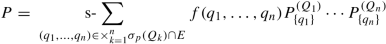
We have the following remarkable result, where we occasionally adopt the notation q := (q ₁, …, q _n) and $\sigma ({\mathfrak Q}):= \times _{k=1}^n \sigma _p(Q_k)$.

Proposition 6.31

Let H be a complex separable Hilbert and suppose that the von Neumann algebra ${\mathfrak R}$ in H satisfies (S1) and (S2). The following facts hold.

• (a) H admits the following Hilbert orthogonal decomposition into closed subspaces, called superselection sectors or coherent sectors ,

  

  (6.7)

  and each H _q is

  • (i) invariant under ${\mathfrak R}$ , i.e. A(H _q) ⊂H _q if $A\in {\mathfrak R}$ ;

  • (ii) irreducible under ${\mathfrak R}$ , i.e. there is no proper, non-trivial ${\mathfrak R}$ -invariant subspace of H _q.

• (b) Correspondingly ${\mathfrak R}$ splits as a direct sum:

  

  (6.8)

  is a von Neumann algebra on the Hilbert space H _q . Finally,

  $$\displaystyle \begin{aligned}{\mathfrak R}_{\mathbf{q}} = {\mathfrak B}({\mathsf H}_{\mathbf{q}}).\end{aligned}$$

• (c) The algebras ${\mathfrak R}_{\mathbf {q}}$ enjoy the following properties.

  • (i) Each map

    

    is a non-faithful (i.e. non-injective) representation of unital ^∗ -algebras of ${\mathfrak R}$ (Definition 2.27 ) which is both strongly and weakly continuous.

  • (ii) Representations associated with distinct values q are unitarily inequivalent: there is no isometric surjective linear map $U: {\mathsf H}_{\mathbf {q}}\to {\mathsf H}_{\mathbf {q}'}$ such that

    

Proof

As the reader can easily prove, since the charges Q _k have pure point spectra and hence each admits a Hilbert basis of eigenvectors, the joint spectral measure $P^{({\mathfrak Q})}$ on ${\mathbb R}^n$ has support given by the closure of $\times _{k=1}^n \sigma _p(Q_k)$ and, if $E \subset {\mathbb R}^n$,

(6.9)

where the spectral projector $P^{(Q_k)}_{\{q_k\}}$, according to Theorem 3.40, is nothing but the orthogonal projector onto the q _k-eigenspace of Q _k. Notice that every $P^{({\mathfrak Q})}_{E}$ is an observable as it belongs to ${\mathfrak R}$. In fact, using Proposition 3.70, $P^{({\mathfrak Q})}_{E}$ commutes with all bounded operators commuting with the PVMs of the Q _k which, by definition, belong to ${\mathfrak R}'$, so that $P^{({\mathfrak Q})}_{E} \in ({\mathfrak R}')'= {\mathfrak R}$. Not only that: as the Q _k commute with the whole ${\mathfrak R}$, we also have $P^{({\mathfrak Q})}_{E} \in {\mathfrak R}'$. In summary $P^{({\mathfrak Q})}_{E} \in {\mathfrak R}\cap {\mathfrak R}'$.

• (a) Since $P^{({\mathfrak Q})}_{\mathbf {q}} P^{({\mathfrak Q})}_{\mathbf {s}} =0$ if q ≠ s and $\sum _{\mathbf {q}\in \sigma _p({\mathfrak Q}) }P^{({\mathfrak Q})}_{\mathbf {q}}=I$, H decomposes as in (6.7). Since $P^{({\mathfrak Q})}_{\mathbf {q}}\in {\mathfrak R}'$, the subspaces of the decomposition are invariant under the action of each element of ${\mathfrak R}$ because $AP^{({\mathfrak Q})}_{\mathbf {q}} = P^{({\mathfrak Q})}_{\mathbf {q}}A$ for every $A\in {\mathfrak R}$, so $A({\mathsf H}_{\mathbf {q}}) = A( P^{({\mathfrak Q})}_{\mathbf {q}}({\mathsf H}_{\mathbf {q}})) = P^{({\mathfrak Q})}_{\mathbf { q}}(A({\mathsf H}_{\mathbf {q}})) \subset {\mathsf H}_{\mathbf {q}}\:.$ Let us pass to irreducibility. Suppose $P \in {\mathfrak R}'\cap {\mathfrak R}$ is an orthogonal projector. Then it must be a function of the Q _k since ${\mathfrak Q}'' = {\mathfrak R}'\cap {\mathfrak R}$ by hypothesis and Proposition 6.23 (H is separable). Therefore

  

  since P = PP ≥ 0 and P = P ^∗. Exploiting measurable functional calculus, we easily find that f(q) = χ _E(q) for some $E \subset \times _{k=1}^n \sigma _p(Q_k)$. In other words P is an element of the joint PVM of ${\mathfrak Q}$: that PVM exhausts all orthogonal projectors in ${\mathfrak R}'\cap {\mathfrak R}$. Now, if {0}≠ K ⊂H _s is an ${\mathfrak R}$-invariant closed subspace, its orthogonal projector P _K must commute with every $A\in {\mathfrak R}$. In fact P _K AP _K = AP _K, and taking the adjoint P _K A ^∗ P _K = P _K A ^∗. But since ${\mathfrak R}$ is ^∗-closed, that reads P _K AP _K = P _K A, for every $A\in {\mathfrak R}$. Comparing the relations found we have AP _K = P _K A. Therefore $P_{\mathsf K} \in {\mathfrak R}'={\mathfrak R}\cap {\mathfrak R}'$ and hence P _K is an element of the PVM $P^{({\mathfrak Q})}$. Furthermore $P_{\mathsf K} \leq P^{({\mathfrak Q})}_{\mathbf {s}}$ because K ⊂H _s. But there are no projectors smaller than $P^{({\mathfrak Q})}_{\mathbf {s}}$ in the PVM of ${\mathfrak Q}$. So $P_{\mathsf K} = P^{({\mathfrak Q})}_{\mathbf {s}}$ and K = H _s.

• (b) is a von Neumann algebra on H _q considered as a Hilbert space in its own right, because this is a strongly closed unital ^∗-subalgebra of ${\mathfrak B}({\mathsf H}_{\mathbf {q}})$. (Observe that $A_{\mathbf {q}} := P^{({\mathfrak Q})}_{\mathbf {q}}AP^{({\mathfrak Q})}_{\mathbf {q}} \in {\mathfrak R}$, and saying $A_n|{ }_{{\mathsf H}_{\mathbf {q}}}\psi \to B\psi$ for all ψ ∈H _q and some $B \in {\mathfrak B}({\mathsf H}_{\mathbf {q}})$ is equivalent to A _{n q} ϕ → B′ϕ for every ϕ ∈H, where B′ extends B by zero on ${\mathsf H}_{\mathbf {q}}^\perp$ and therefore defines an element of ${\mathfrak B}({\mathsf H})$. Since ${\mathfrak R}$ is a von Neumann algebra, $B'\in {\mathfrak R}$ and $B\in {\mathfrak R}_{\mathbf {q}}$.) Formula (6.8) holds by definition. Since H _q is ${\mathfrak R}$-irreducible it is evidently irreducible also under ${\mathfrak R}_{\mathbf {q}}$ by construction. Schur’s lemma (Theorem 6.19) implies that ${\mathfrak R}_{\mathbf {q}}^{\prime \prime } = {\mathfrak B}({\mathsf H}_{\mathbf {q}})$. As ${\mathfrak R}_{\mathbf {q}}^{\prime \prime }={\mathfrak R}_{\mathbf {q}}$ since we are dealing with a von Neumann algebra, necessarily ${\mathfrak R}_{\mathbf {q}} = {\mathfrak B}({\mathsf H}_{\mathbf {q}})$.

• (c) Each map is a strongly and weakly continuous representation of unital ^∗-algebras, as we can check directly. This representation cannot be faithful, because for instance $P^{({\mathfrak Q})}_{\mathbf {q}}\in {\mathfrak R}$ is represented by the zero operator on ${\mathsf H}_{\mathbf {q}'}$ if q ′≠ q. Furthermore, if q ≠ q ′—say $q_1 \neq q_1^{\prime }$—there is no isometric surjective linear map $U: {\mathsf H}_{\mathbf {q}}\to {\mathsf H}_{\mathbf {q}'}$ such that . If such an operator existed one would have $q_1I_{{\mathsf H}_{\mathbf {q}'}} = U Q_1|{ }_{{\mathsf H}_{\mathbf {q}}} U^{-1} = Q_1|{ }_{{\mathsf H}_{\mathbf {q}'}} =q_1^{\prime }I_{{\mathsf H}_{\mathbf {q}'}}$ so that $q_1=q^{\prime }_1$. (If Q ₁ is unbounded it suffices to consider the central bounded operator $Q_{1n} = \int _{[-n,n]} r dP^{(Q_1)}(r)$ with [−n, n] ∋ q ₁, q ₂.)

□

We have found that in presence of superselection charges the Hilbert space decomposes into pairwise orthogonal subspaces which are invariant and irreducible under the algebra of observables, thus giving rise to inequivalent representations of the algebra itself. There exist several superselection structures in physics beside the one we pointed out. The three most renowned ones are very different in nature (see Examples 6.32 and 7.19):

• the superselection structure of the electric charge,

• the superselection structure of integer/semi-integer angular momenta,

• the superselection rule of the mass in non-relativistic physics, i.e. Bargmann’s superselection rule.

These superselection rules take place simultaneously and can be described by pairwise compatible superselection charges so that the picture above is valid. Notice that, in each superselection sector, the physical description is essentially identical to the naive one where every selfadjoint operator is an observable (namely ${\mathfrak R} = {\mathfrak B}({\mathsf H})$) and the superselection charges appear just in terms of fixed parameters.

Example 6.32

The electric charge is the typical example of a superselection charge. For instance, referring to an electron the Hilbert space is $L^2({\mathbb R}^3, d^3x)\otimes {\mathsf H}_{s}\otimes {\mathsf H}_{e}$. The space of the electric charge is ${\mathsf H}_e= {\mathbb C}^2$, on which Q = eσ _z (see (1.12)). In principle several other observables could exist on H _e, but the electric charge’s superselection rule imposes that the only possible observables commute with Q and are functions of σ ₃. The centre of the algebra of observables is I ⊗ I ⊗ f(σ ₃) for every function $f : \sigma (\sigma _3) = \{-1,1\} \to {\mathbb C}$. We have the decomposition into coherent sectors

$$\displaystyle \begin{aligned}{\mathsf H} = (L^2({\mathbb R}^3, d^3x)\otimes {\mathsf H}_{s}\otimes {\mathsf H}_+ ) \bigoplus (L^2({\mathbb R}^3, d^3x)\otimes {\mathsf H}_{s}\otimes {\mathsf H}_-)\:,\end{aligned}$$

where H _± are the eigenspaces of Q relative to eigenvalues ± e, respectively. $\blacksquare$

Remark 6.33

A fundamental requirement is that the superselection charges have pure point spectra. If instead ${\mathfrak R}\cap {\mathfrak R}'$ contains an operator A having a continuous part in its spectrum with non-empty interior (A may also be the strong limit on D(A) of a sequence of elements in ${\mathfrak R}\cap {\mathfrak R}'$), the proposition does not hold, and H cannot be decomposed in a direct sum of closed subspaces. In this case it decomposes as a direct integral: this produces a much more complicated structure, whose physical meaning seems dubious. $\blacksquare$

6.3.2 Global Gauge Group Formulation and Non-Abelian Superselection

There are quantum physical systems with von Neumann algebra of observables ${\mathfrak R}$ for which ${\mathfrak R}'$ is not Abelian (think of chromodynamics, where ${\mathfrak R}'$ contains a faithful representation of SU(3)). In that case the centre of ${\mathfrak R}$ does not retain the full information about ${\mathfrak R}'$. A primary notion is here the group of unitary operators called the commutant group of ${\mathfrak R}$ (introduced in [JaMi61] and called gauge group there):

$$\displaystyle \begin{aligned}{\mathfrak G}_{\mathfrak R} := \{V\in {\mathfrak R}' \:|\: V\mbox{ is unitary}\}\:.\end{aligned}$$

It holds all the information about ${\mathfrak R}$ and ${\mathfrak R}'$ because (making use of ${\mathfrak R}''={\mathfrak R}$ and Proposition 3.55)

$$\displaystyle \begin{aligned} \begin{array}{rcl} {\mathfrak G}_{\mathfrak R}^{\prime}= {\mathfrak R}\quad \mbox{and} \quad {\mathfrak G}_{\mathfrak R}^{\prime\prime} = {\mathfrak R}'\:.{}\end{array} \end{aligned} $$

(6.10)

In the presence of Abelian superselection rules, ${\mathfrak G}_{\mathfrak R}$ is Abelian (${\mathfrak G}_{\mathfrak R} \subset {\mathfrak R}' ={\mathfrak R}\cap {\mathfrak R}'$). Similarly to (6.10), ${\mathfrak R}$ can be extracted from ${\mathfrak B}({\mathsf H})$: one employs the former in (6.10) and uses a subgroup of ${\mathfrak G}_{\mathfrak R}$ constructed out of a set of physically meaningful superselection charges Q ₁, …, Q _n. $A \in {\mathfrak R}$ if and only if A commutes with the PVMs of Q ₁, …, Q _n. Decomposing $A= \frac {1}{2}(A+A^*) + i\frac {1}{2i}(A-A^*)$ and exploiting Proposition 3.70, this is equivalent to saying

$$\displaystyle \begin{aligned} \begin{array}{rcl} U_{\mathbf{s}} A = A U_{\mathbf{s}}\:, \quad U_{\mathbf{s}} := e^{is_1Q_1}\cdots e^{is_nQ_n}\quad \mbox{for }\mathbf{s} :=(s_1,\ldots, s_n) \in {\mathbb R}^n{}\end{array} \end{aligned} $$

(6.11)

where $U: {\mathbb R}^n \ni \mathbf {s} \mapsto U_{\mathbf {s}}$ is a strongly-continuous unitary representation of the Abelian topological group ${\mathbb R}^n$ taking values in ${\mathfrak G}_{\mathfrak R}$. Looking at Remark 6.30, the occurrence of Abelian discrete superselection rules can be condensed in three facts: (a) H is separable, (b) Q ₁, …, Q _n have pure point spectra, and (c)

$$\displaystyle \begin{aligned} \begin{array}{rcl} {\mathfrak R} = U({\mathbb R}^n)'\:.{}\end{array} \end{aligned} $$

(6.12)

Observe that $U({\mathbb R}^n)$ is considerably smaller than ${\mathfrak G}_{\mathfrak R}$, since other choices for the charges Q _k and also for their number are possible. These would produce other subgroups of ${\mathfrak G}_{\mathfrak R}$ still satisfying (6.12): it is sufficient that the joint PVM of these charges is made of the same projectors P _q onto the sectors determined by the initial charges. We can do better if we use the separability of H: namely, out of the PVMs of the n charges Q _k we can construct the unique charge

$$\displaystyle \begin{aligned}Q:= s\mbox{-}\sum_{\mathbf{q}\in \sigma({\mathfrak Q})}m_{\mathbf{q}} P_{\mathbf{q}}\:,\end{aligned}$$

for some injective map $\mathbf {q} \mapsto m_{\mathbf {q}} \in {\mathbb Z}$, which must exist because there are at most countably many PVMs P _q, since H is separable. Now, by Remark 6.30 and Proposition 3.70, the representation U of ${\mathbb R}^n$ in (6.12) can be replaced by a faithful and strongly-continuous representation of the compact Abelian group U(1),

$$\displaystyle \begin{aligned} \begin{array}{rcl} {} U: U(1) \ni e^{is} \mapsto e^{isQ} \in {\mathfrak G}_{\mathfrak R}\:.\end{array} \end{aligned} $$

(6.13)

We stress that (6.13) is well defined and is a representation of U(1), not only of ${\mathbb R}$, simply because $\sigma (Q) \subset {\mathbb Z}$. (The charge Q has, however, no direct physical meaning in general, except perhaps for n = 1 with Q = e ⁻¹ Q ₁, where Q ₁ is the electric charge and e the elementary electric charge.) The splittings (6.7)–(6.8) hold and every ${\mathfrak R}$-invariant and ${\mathfrak R}$-irreducible closed subspace H _q is U-invariant too, since is a pure phase (however U-irreducibility fails unless $\dim ({\mathsf H}_{\mathbf {q}})=1$).

In the non-Abelian case, decompositions similar to (6.7)–(6.8) are expected to hold with reference to a strongly-continuous faithful representation $U: G \ni g \mapsto U_g \in {\mathfrak G}_{\mathfrak R}$ of some (compact) group G, called the global gauge group, such that $U'= {\mathfrak G}_{\mathfrak R}^{\prime } = {\mathfrak R}$ (here, and occasionally henceforth, U′ := U(G)′):

$$\displaystyle \begin{aligned} \begin{array}{rcl} {\mathsf H} = \bigoplus_{\chi \in K} {\mathsf H}_\chi\:, \quad {\mathfrak R} = \bigoplus_{\chi \in K} {\mathfrak R}_\chi\:, \quad U_g = \bigoplus_{\chi \in K} U^{(\chi)}_g\:.{}\end{array} \end{aligned} $$

(6.14)

Above, H _χ is a non-trivial closed subspace that is both ${\mathfrak R}$-invariant and U-invariant, determining corresponding (non-faithful, strongly and weakly continuous) representations

(6.15)

where the commutant refers to ${\mathfrak B}({\mathsf H}_\chi )$.

The fundamental difference with the Abelian case is that now ${\mathfrak R}_\chi$ is only a factor in ${\mathfrak B}({\mathsf H}_\chi )$ rather than the entire ${\mathfrak B}({\mathsf H}_\chi )$:

$$\displaystyle \begin{aligned} \begin{array}{rcl} {\mathfrak R}_\chi \cap {\mathfrak R}_\chi' = {\mathbb C} I_\chi = (U^{(\chi)})'\cap (U^{(\chi)})''\quad \mbox{for every }\chi\in K\:.{}\end{array} \end{aligned} $$

(6.16)

If everything we stated holds, the orthogonal projectors P _χ onto every subspace H _χ must commute with U and ${\mathfrak R}$, so they belong to the centre ${\mathfrak R} \cap {\mathfrak R}' = U' \cap U''$. Using the projectors P _χ we can still construct superselection charges whose joint PVM determines the generalized superselection sectors H _χ.

We have in fact the following general result where separability is not necessary.

Proposition 6.34

Let ${\mathfrak R}$ be a von Neumann algebra on the Hilbert space H ≠ {0}. Suppose there exists a faithful, strongly-continuous unitary representation $U: G \ni g \mapsto U_g \in {\mathfrak G}_{{\mathfrak R}}$ of the compact Hausdorff group G such that $U(G)'= {\mathfrak R}$ . Then

• (a) (6.14)–(6.16) hold, where K is a set of equivalence classes of irreducible strongly-continuous and unitarily-equivalent representations of G,

• (b) ${\mathfrak R}_\chi$ and ${\mathfrak R}_{\chi '}$ are unitarily inequivalent if χ ≠ χ′.

Proof

(a) Let us start by proving (6.14). If G is Hausdorff and compact, as G ∋ g↦U _g is strongly continuous, the Peter-Weyl Theorem (Theorem 7.35) gives an orthogonal Hilbert decomposition H =⊕_{χ ∈ K} H _χ where each H _χ is non-trivial, closed and U-invariant. K labels equivalence classes of irreducible strongly-continuous unitarily-equivalent representations of G. In particular we have a finer Hilbert orthogonal decomposition: ${\mathsf H}_\chi = \bigoplus _{\lambda \in \Lambda _\chi } {\mathsf H}^{(\lambda )}_\chi$, where every closed subspace ${\mathsf H}^{(\lambda )}_\chi$ is U-invariant, every restriction is finite-dimensional and irreducible, and the U ^(χλ) are unitarily equivalent as λ ∈ Λ_χ varies, for every fixed χ. By direct inspection, using the irreducibility and unitary equivalence of the U ^(χλ) for fixed χ, one finds $(U^{(\chi )})'' \cap (U^{(\chi )})' = {\mathbb C} I$, where the commutant is referred to H _χ. On the other hand, since the U ^(χ) with different χ are unitarily inequivalent and $U' = {\mathfrak G}_{\mathfrak R}^{\prime }= {\mathfrak R}$, every H _χ is ${\mathfrak R}$-invariant and the subrepresentation ${\mathfrak R}_\chi$ obtained by restriction satisfies ${\mathfrak R}_\chi = (U^{(\chi )})'$ where the commutant is referred to H _χ. In particular ${\mathfrak R}_\chi$ is a von Neumann algebra on H _χ. Hence $(U^{(\chi )})' \cap (U^{(\chi )})'' = {\mathbb C} I$ can be translated into ${\mathfrak R}_\chi \cap {\mathfrak R}_\chi ' = {\mathbb C} I$, and every ${\mathfrak R}_\chi$ is a factor, proving (6.16). (b) Let $P_\chi , P_{\chi '}\in {\mathfrak R}\cap {\mathfrak R}'$ be the orthogonal projectors onto H _χ and ${\mathsf H}_{\chi '}$ respectively, with χ ≠ χ′. We claim ${\mathfrak R}_\chi$, ${\mathfrak R}_{\chi '}$ are unitarily inequivalent. If there were an isometric surjective map $V: {\mathsf H}_\chi \to {\mathsf H}_{\chi '}$ with , we would find when representing the operator $A= P_\chi - P_{\chi '} \in {\mathfrak R}$. □

For Abelian discrete superselection rules, the existence of a global compact gauge group G as in the theorem is guaranteed by the separability of H, as we established above for G = U(1). In this case, decomposition (6.14) coincides with (6.7)–(6.8); additionally, we know that ${\mathfrak R}_\chi = {\mathfrak B}({\mathsf H}_\chi )$ and U ^(χ) is a pure phase. If ${\mathfrak G}_{\mathfrak R}$ is not Abelian the issue of whether such a G exists has to be examined case by case. In all physically interesting cases, G is a compact Lie group (hence a matrix group) and U(G) is considerably smaller than ${\mathfrak G}_{\mathfrak R}$.

The approach to superselection rules based on the notion of a global compact gauge group of internal symmetries G turns out to be powerful and deep if used in addition to the request of spacetime locality in algebraic quantum field theory in Minkowski spacetime formulated in terms of von Neumann algebras. These remarkable results are due to several authors and rely on the so-called Doplicher-Haag-Roberts (DHR) analysis and the Buchholz-Fredenhagen (BF) analysis of superselection sectors [Haa96] describing theories with short-range interactions and without topological charges in BF sense. A rather complete technical review including fundamental references is [HaMü06].

6.3.3 Quantum States in the Presence of Abelian Superselection Rules

Let us come to the problem of characterizing states when an Abelian superselection structure is turned on a complex separable Hilbert space H, in accordance with (S1) and (S2). In principle, we can extend Definition 4.43 given for ${\mathfrak R}$ with trivial centre. As usual ${\mathcal {L}}_{{\mathfrak R}}({\mathsf H})$ indicates the lattice of orthogonal projectors on ${\mathfrak R}$, which we know to be bounded by 0 and I, orthocomplemented, σ-complete, orthomodular and separable. It is not atomic and it does not satisfy the covering property in general. The atoms are one-dimensional projectors, exactly as pure states when ${\mathfrak R} = {\mathfrak B}({\mathsf H})$, so we should expect some differences when ${\mathfrak R} \neq {\mathfrak B}({\mathsf H})$. We start from the following general definition, valid also if H is not separable.

Definition 6.35

Let H be a complex Hilbert space. A quantum probability measure relative to the von Neumann algebra ${\mathfrak R}\subset {\mathfrak B}({\mathsf H})$, is a map $\rho : {\mathcal {L}}_{{\mathfrak R}}({\mathsf H}) \to [0,1]$ satisfying the following requirements:

• (1) ρ(I) = 1 .

• (2) If $\{Q_n\}_{n \in N}\subset {\mathcal {L}}_{{\mathfrak R}}({\mathsf H})$, N at most countable, satisfies Q _k ⊥ Q _h = 0 when h, k ∈ N, then

  $$\displaystyle \begin{aligned} \begin{array}{rcl} \rho(\vee_{k\in N}Q_k) = \sum_{k \in N} \rho(Q_k)\:.{}\end{array} \end{aligned} $$

  (6.17)

The set of the quantum probability measures relative to ${\mathfrak R}$ will be denoted by $\mathcal {M}_{{\mathfrak R}}({\mathsf H})$. $\blacksquare$

Remark 6.36

Provided N is at most countable, $\vee _{k\in N}Q_k\in {\mathcal {L}}_{{\mathfrak R}}({\mathsf H})$ if every $Q_k \in {\mathcal {L}}_{{\mathfrak R}}({\mathsf H})$, because this lattice is σ-complete (even if H is not separable). Without this fact the definition above would be meaningless. $\blacksquare$

Recall that a von Neumann algebra ${\mathfrak R}$ is strongly closed, and the strong topology is the one used to manipulate operators spectrally. Moreover A = A ^∗ is affiliated or belongs to ${\mathfrak R}$ if and only if its PVM belongs to $\mathcal {L}_{\mathfrak R}({\mathsf H})$. Because of all this the definitions of Sect. 4.5.1 can be given also in the presence of Abelian superselection rules, and they give a meaning to notions like the expectation value and standard deviation of an observable for a given quantum state viewed as a probability measure on $\mathcal {L}_{\mathfrak R}({\mathsf H})$.

The procedures presented in Sect. 4.5.1 to compute those statistical objects in terms of traces make sense when the quantum probability measures are represented by trace-class operators. This is possible also when we have superselection rules, as we shall prove, even if the picture is more complicated.

Assuming H separable, if there is an Abelian superselection structure, we can write simpler-looking decompositions:

$$\displaystyle \begin{aligned} \begin{array}{rcl} {\mathsf H} = \bigoplus_{k\in K} {\mathsf H}_{k} \:, \quad {\mathfrak R} = \bigoplus_{k\in K} {\mathfrak R}_{k}\:, \quad {\mathfrak R}_{k} = {\mathfrak B}({\mathsf H}_k)\:, \: k \in K{}\end{array} \end{aligned} $$

(6.18)

where K is some finite or countable set. The lattice ${\mathcal {L}}_{{\mathfrak R}}({\mathsf H})$, as a consequence of (6.17), splits as (the notation should be obvious)

$$\displaystyle \begin{aligned} \begin{array}{rcl} {\mathcal{L}}_{{\mathfrak R}}({\mathsf H}) = \bigoplus_{k\in K} {\mathcal{L}}_{{\mathfrak R}_k}({\mathsf H}_k) = \bigoplus_{k\in K} {\mathcal{L}}({\mathsf H}_k) \end{array} \end{aligned} $$

(6.19)

where ${\mathcal {L}}_{{\mathfrak R}_k}({\mathsf H}_k) \cap {\mathcal {L}}_{{\mathfrak R}_h}({\mathsf H}_h) = \{0\} \quad \mbox{if }k\neq h$.

In other words $Q \in {\mathcal {L}}_{{\mathfrak R}}({\mathsf H})$ can be written uniquely as Q = ⊕_{k ∈ K} Q _k where $Q_k \in {\mathcal {L}}({\mathfrak B}({\mathsf H}_k))$. In fact Q _k = P _k Q, where P _k is the orthogonal projector onto H _k.

Let us focus on the problem of characterizing quantum probability measures in terms of trace-class operators and unit vectors up to phase.

Remark 6.37

We shall avoid using already introduced terms like mixed states and pure states which correspond, in the absence of superselection rules, to quantum-state operators (positive trace-class operators of unit trace) and unit vectors modulo phase, respectively. We shall explain in a short while that these mathematical objects do not (yet) correspond one-to-one with extremal quantum probability measures and generic quantum probability measures. Physically, speaking, the safest approach is to assume that quantum states are nothing but quantum probability measures. $\blacksquare$

It is possible to adapt Gleason’s result simply by observing that $\rho \in \mathcal {M}_{\mathfrak R}({\mathsf H})$ defines an analogous quantum probability measure ρ _k on ${\mathcal {L}}_{{\mathfrak R}_k}({\mathsf H}_k) = {\mathcal {L}}({\mathsf H}_k)$ by

$$\displaystyle \begin{aligned}\rho_k (P) := \frac{1}{\rho(P_k)} \rho(P)\:, \quad P \in {\mathcal{L}}({\mathsf H}_k)\:,\end{aligned}$$

provided ρ(P _k) ≠ 0. If $\dim ({\mathsf H}_k)\neq 2$ we can exploit Gleason’s theorem. According to Proposition 4.45, the set $\mathcal {S}({\mathsf H})$ of quantum-state operators on H contains all operators $T \in {\mathfrak B}_1({\mathsf H})$ satisfying T ≥ 0 and tr(T) = 1.

Theorem 6.38

Let H be a complex separable Hilbert space, and assume that the von Neumann algebra ${\mathfrak R}$ on H satisfies (S1) and (S2). In the ensuing coherent decomposition (6.18) we suppose $\dim {\mathsf H}_k \neq 2$ for every k ∈ K. Then the following facts hold.

• (a) If $T\in \mathcal {S}({\mathsf H})$ , then $\rho _T \in \mathcal {M}_{{\mathfrak R}}({\mathsf H})$ if

  $$\displaystyle \begin{aligned}\rho_T : {\mathcal{L}}_{{\mathfrak R}}({\mathsf H}) \ni P \mapsto tr(T P)\:.\end{aligned}$$

• (b) For $\rho \in \mathcal {M}_{{\mathfrak R}}({\mathsf H})$ there exists $T \in \mathcal {S}({\mathsf H})$ such that ρ = ρ _T.

• (c) If $T_1, T_2 \in \mathcal {S}({\mathsf H})$ , then $\rho _{T_1}=\rho _{T_2}$ if and only if P _k T ₁ P _k = P _k T ₂ P _k for all k ∈ K, P _k being the orthogonal projector onto H _k.

• (d) A unit vector ψ ∈H defines an extremal measure if and only if it belongs to a coherent sector. More precisely, a measure $\rho \in \mathcal {M}_{{\mathfrak R}}({\mathsf H})$ is extremal if and only if there exist k ₀ ∈ K and a unit vector $\psi \in {\mathsf H}_{k_0}$ such that

  $$\displaystyle \begin{aligned}\rho(P)=0 \quad \mathit{\mbox{if }}P \in {\mathcal{L}}({\mathsf H}_{k}), k\neq k_0 \quad \mathit{\mbox{ and }}\quad \rho(P) = \langle \psi|P \psi \rangle\mathit{\mbox{ if }}P \in {\mathcal{L}}({\mathsf H}_{k_0})\end{aligned}$$

Proof

(a) is obvious from Proposition 4.45, as the restriction to ${\mathcal {L}}_{{\mathfrak R}}({\mathsf H})$ of a quantum probability measure ρ on ${\mathcal {L}}({\mathsf H})$ is a similar measure. Let us prove (b). Evidently, every $\rho |{ }_{{\mathcal {L}}({\mathsf H}_k)}$ is a positive measure with 0 ≤ ρ(P _k) ≤ 1. We can apply Gleason’s theorem to find a positive $T_k\in {\mathfrak B}({\mathsf H}_k)$ with tr(T _k) = ρ(P _k) such that ρ(Q) = tr(T _k Q) if $Q\in {\mathcal {L}}({\mathsf H}_k)$. Notice also that ||T _k||≤ ρ(P _k) because

$$\displaystyle \begin{aligned}||T_k||= \sup_{\lambda \in \sigma_p(T_k)} |\lambda| = \sup_{\lambda \in \sigma_p(T_k)} \lambda \leq \sum_{\lambda \in \sigma_p(T_k)} d_\lambda \lambda = tr(T_k) = \rho(P_k)\:.\end{aligned}$$

If $Q \in {\mathcal {L}}_{{\mathfrak R}}({\mathsf H})$, Q =∑_k Q _k, where $Q_k:= P_kQ \in {\mathcal {L}}({\mathsf H}_k)$, Q _k Q _h = 0 if k ≠ h. Therefore by σ-additivity

$$\displaystyle \begin{aligned}\rho(Q)= \sum_k \rho(Q_k) = \sum_k tr(T_kQ_k)\end{aligned}$$

since H _k ⊥H _h, which can be written ρ(Q) = tr(TQ) for $T := \oplus _{k}T_k\in {\mathfrak B}_1({\mathsf H})$. It is clear that $T \in {\mathfrak B}({\mathsf H})$ because, if x =∑_k x _k, x _k ∈H _k, is a unit vector, then ||Tx||≤∑_k||T _k|| ||x _k||≤∑_k||T _k||1 ≤∑_k ρ(P _k) = 1. In particular ||T||≤ 1. T ≥ 0 because each T _k ≥ 0. Hence $|T| = \sqrt {T^*T} = \sqrt {TT} = T$ via functional calculus, and also |T _k| = T _k. Moreover, using the spectral decomposition of T, whose PVM commutes with each P _k, one easily has |T| = ⊕_k|T _k| = ⊕_k T _k. The condition

$$\displaystyle \begin{aligned}1= \rho(I) =\sum_k \rho(P_k) = \sum_k tr(T_kP_k)= \sum_k tr(|T_k|P_k)\end{aligned}$$

is equivalent to saying tr |T| = 1, using a Hilbert basis of H made of the union of bases in each H _k. We have obtained, as we wanted, that $T \in {\mathfrak B}_1({\mathsf H})$, T ≥ 0, tr(T) = 1 and ρ(Q) = tr(TQ) for all $Q \in {\mathcal {L}}_{{\mathfrak R}}({\mathsf H})$.

(c) The proof is straightforward from ${\mathcal {L}}_{{\mathfrak R}_k}({\mathsf H}_k) = {\mathcal {L}}({\mathfrak B}({\mathsf H}_k))$, because ${\mathfrak R}_k = {\mathfrak B}({\mathsf H}_k)$ and, evidently, $\rho _{T_1} = \rho _{T_2}$ if and only if for all k ∈ K.

(d) It is clear that if ρ has more than one component, $\rho |{ }_{{\mathcal {L}}({\mathsf H}_k)}\neq 0$ cannot be extremal because it is, by construction, a convex combination of other states which vanish on some of the coherent subspaces. Therefore only states such that only one restriction does not vanish may be extremal. Now Proposition 4.51 (a) implies that among these states the extremal ones are precisely those of the form claimed in (d). □

Remark 6.39

• (a) Take ψ =∑_{k ∈ K} c _k ψ _k where the ψ _k ∈H _k are unit vectors, and suppose ||ψ||² =∑_k|c _k|² = 1. This vector induces a state ρ _ψ on ${\mathfrak R}$ by means of the standard procedure (which is merely a trace with respect to T _ψ := 〈ψ| 〉ψ)

  $$\displaystyle \begin{aligned}\rho_\psi(P) = \langle \psi|P \psi \rangle \quad P \in {\mathcal{L}}_{{\mathfrak R}}({\mathsf H})\:.\end{aligned}$$

  In this case however, since PP _k = P _k P and ψ _k = P _k ψ _k, we have

  $$\displaystyle \begin{aligned} \rho_\psi(P) &= \langle \psi|P \psi \rangle = \sum_{k}\sum_h \overline{c_k}c_h \langle \psi_k|P \psi_k \rangle\\ & = \sum_{k}\sum_h \overline{c_k}c_h \langle P_k\psi_k|PP_h \psi_k \rangle = \sum_{k}\sum_h \overline{c_k}c_h \langle \psi_k|P_kPP_h \psi_h \rangle\\ &= \sum_{k}\sum_h \overline{c_k}c_h \langle \psi_k|PP_kP_h \psi_k \rangle =\sum_{k}\sum_h \overline{c_k}c_h \langle \psi|PP_k \psi \rangle\delta_{kh}\\ &= \sum_k |c_k|{}^2 \langle \psi_k|P \psi_k \rangle = tr(T^{\prime}_\psi P)\end{aligned} $$

  where

  $$\displaystyle \begin{aligned}T^{\prime}_\psi = \sum_{k\in K} |c_k|{}^2 \langle \psi_k | \:\: \rangle \psi_k\:.\end{aligned}$$

  We conclude that the apparent pure state described by the vector ψ and the apparent mixed state described by the operator $T^{\prime }_\psi$ cannot be distinguished, simply because the algebra ${\mathfrak R}$ is too small to distinguish between them. Actually they define the same probability measure, i.e. the same quantum state, and this is an elementary case of (c) in the above theorem, with T ₁ = 〈ψ| 〉ψ and $T_2= T^{\prime }_\psi$. This fact is often stated as follows in the argot of physicists:

  no coherent superpositions ψ =∑_{k ∈ K} c _k ψ _k of pure states ψ _k ∈H _k from different coherent sectors are possible; only incoherent superpositions ∑_{k ∈ K}|c _k|²〈ψ _k| 〉ψ _k are allowed.

• (b) It should be clear that the one-to-one correspondence between extremal quantum measures and atomic elementary observables (one-dimensional projectors) here does not work. Consequently, notions like the probability amplitude must be handled with great care. In general, however, everything pans out—correspondence included—if one stays in a fixed superselection sector H _k.

• (c) We leave to the reader the easy proof of the fact that the Lüders-von Neumann postulate on post-measurement states (see Sect. 4.4.7) can be stated as it stands also in the presence of superselection rules, no matter which $T\in \mathcal {S}({\mathsf H})$ we use to describe a quantum probability measure ρ: the post-measurement probability measure ρ′ does not depend on the chosen representation of ρ by operators. Besides, it is worth stressing that since the PVM of an observable in ${\mathfrak R}$ (or affiliated to ${\mathfrak R}$) commutes with the central projectors P _k defining the superselection sectors H _k, if an extremal quantum state is initially represented by a vector belonging to a sector H _k, there is no chance to leave that sector by means of a subsequent measurement of any observable in ${\mathfrak R}$. $\blacksquare$

Example 6.40

Going back to Example 6.32, states (probability measures on $\mathcal {L}_{\mathfrak R}({\mathsf H})$) where Q takes the value − e with probability 1 are said states of electrons. When Q takes the value + e with probability 1 one talks about states of positrons, to be absolutely thorough. However, as soon as we measure Q, its value cannot later change due to measurements of other observables, since all physically meaningful observables commute with Q and the postulate of collapse leaves the state in the initial eigenspace of Q. This means that once the charge has been observed and the particle is baptized an electron or a positron, from that moment on it is impossible to put the system in a state where the value of Q is not defined and the particle is in an electron-positron superposition. In principle it could still be possible to put the system into a similar superposed state in view of time evolution. This is not the case however, since the conservation law of the electrical charge stipulates that the observable Q is a constant of motion. $\blacksquare$

6.3.4 The General Case ${\mathfrak R} \subset {\mathfrak B}({\mathsf H})$: Quantum Probability Measures, Normal and Algebraic States

Let us finally focus on the various notions of quantum state one can adopt in the completely general setup ${\mathfrak R} \subset {\mathfrak B}({\mathsf H})$, where H is not necessarily separable, and introduce the relevant terminology. In principle, amongst other possibilities, one can always define states in terms of quantum probability measures on $\mathcal {L}_{\mathfrak R}({\mathsf H})$, so that they form the convex body $\mathcal {M}_{\mathfrak R}({\mathsf H})$. In particular, due to Proposition 4.45, quantum state operators $T\in \mathcal {S}({\mathsf H})$ still represent (certain) quantum probability measures in the sense of Definition 6.35, namely σ-additive probability measures in $\mathcal {M}_{\mathfrak R}({\mathsf H})$. Obviously T and T′ := V TV ⁻¹, where $V \in {\mathfrak G}_{\mathfrak R}$, define the same measure if the global gauge group ${\mathfrak G}_{\mathfrak R}$ is not trivial (represented by pure phases), because

$$\displaystyle \begin{aligned}tr(AVTV^{-1})= tr(V^{-1}AVT)= tr(AV^{-1}VT)= tr(AT)\:, \quad \mbox{if }A\in {\mathfrak R}.\end{aligned}$$

So there are many ways to describe the same state in terms of quantum-state operators, and a meaningful definition of pure quantum states is again provided by extremal elements of $\mathcal {M}_{\mathfrak R}({\mathsf H})$, if any, rather than unit vectors.

Let us pass to the converse problem: can all σ-additive probability measures in $\mathcal {M}_{\mathfrak R}({\mathsf H})$ be written in terms of quantum-state operators, i.e., positive trace-class operators of trace one in the generic case ${\mathfrak R} \subset {\mathfrak B}({\mathsf H})$? The answer is only partially positive [Dvu92, Ham03].

• (1) If H is separable, and assuming that the type decomposition of ${\mathfrak R}$ does not include type-I ₂ summands, Gleason’s theorem still holds: positive trace-class operators of unit trace represent all σ-additive probability measures on $\mathcal {L}_{\mathfrak R}({\mathsf H})$, with the caveat that several distinct operators may represent the same measure if ${\mathfrak R} \subsetneq {\mathfrak B}({\mathsf H})$.

• (2) If H is not separable, and again dispensing with type-I ₂ factors in ${\mathfrak R}$, then positive trace-class operators of trace one represent all completely additive probability measures on $\mathcal {L}_{\mathfrak R}({\mathsf H})$ but only them. The latter’s set is denoted by $\mathcal {M}_{\mathfrak R}({\mathsf H})_{ca}$, cf. Remark 4.46. Again the proviso holds that many operators may represent the same measure if ${\mathfrak R} \subsetneq {\mathfrak B}({\mathsf H})$.

Notice that $\mathcal {M}_{\mathfrak R}({\mathsf H})_{ca} \subset \mathcal {M}_{\mathfrak R}({\mathsf H})$, with equality if and only if H is separable, for otherwise $\mathcal {M}_{\mathfrak R}({\mathsf H})_{ca}$ is properly included in $\mathcal {M}_{\mathfrak R}({\mathsf H})$. So, if we want to work with von Neumann algebras on non-separable Hilbert spaces with the intent to describe quantum states in terms of probability measures, it might be convenient to redefine quantum probability measures by restricting to the completely-additive ones if we also wish that these measures are represented by quantum-state operators. A far-reaching discussion on the structure of additive measures on von Neumann algebras in terms of operators can be found in [Ham03].

There is an alternative definition of quantum states on ${\mathfrak R}$ that does not identify them to (σ/completely-additive) probability measures on $\mathcal {L}_{\mathfrak R}({\mathsf H})$, but still captures all probability measures (σ/completely-additive) induced by quantum-state operators: these are the algebraic states. We will discuss the concept further in the last chapter, motivating its necessity in a more general context.

Definition 6.41

Let ${\mathfrak R}$ be a von Neumann algebra on H.

• (1) An algebraic state on ${\mathfrak R}$ is a linear map $\omega : {\mathfrak R} \to {\mathbb C}$ such that ω(I) = 1 and ω(A ^∗ A) ≥ 0 if $A\in {\mathfrak R}$

• (2) The algebraic states ω _T induced by quantum-state operators $T\in \mathcal {S}({\mathsf H})$:

  $$\displaystyle \begin{aligned}\omega_T(A) := tr(TA)\quad \mbox{ for }A\in {\mathfrak R},\end{aligned}$$

  are called normal (algebraic) states of ${\mathfrak R}$, and their set is the folium of ${\mathfrak R}$. A pure normal state is an extremal element of the convex body of normal states on ${\mathfrak R}$. $\blacksquare$

Remark 6.42

• (a) We stress that the map associating $T\in \mathcal {S}({\mathsf H})$ to the algebraic state $\omega _T:{\mathfrak R} \to {\mathbb C}$ is very far from being injective in general (it depends on how big ${\mathfrak R}$ is).

• (b) If ${\mathfrak R}={\mathfrak B}({\mathsf H})$ (also with H non-separable), as we already know, the set of pure normal states coincides with the set of vector states T = 〈ψ|⋅〉ψ for unit vectors ψ ∈H. For smaller von Neumann algebras this fact is usually false.

• (c) From the standpoint of the measure theory on $\mathcal {L}_{\mathfrak R}({\mathsf H})$, algebraic states define additive, but not necessarily σ-additive or completely additive probability measures. The set of additive measures on $\mathcal {L}_{\mathfrak R}({\mathsf H})$ is denoted by $\mathcal {M}_{\mathfrak R}({\mathsf H})_{a}$. Evidently $\mathcal {M}_{\mathfrak R}({\mathsf H})_{a}\supset \mathcal {M}_{\mathfrak R}({\mathsf H}) \supset \mathcal {M}_{\mathfrak R}({\mathsf H})_{ca}$.

• (d) Normal states are defined even if ${\mathfrak R}$ does contain type-I ₂ summands. In this case, however, they are not able to capture all completely-additive probability measures on $\mathcal {L}_{\mathfrak R}({\mathsf H})$.

• (e) Suppose $\rho \in \mathcal {M}_{\mathfrak R}({\mathsf H})_a$ and ${\mathfrak R}$ is free of type-I ₂ summands. If there exists $P\in \mathcal {L}_{\mathfrak R}({\mathsf H})$ such that ρ(Q) = 0 for $Q\in \mathcal {L}_{\mathfrak R}({\mathsf H})$ iff PQ = QP = 0, then P is called the support of ρ. It turns out that $\rho \in \mathcal {M}_{\mathfrak R}({\mathsf H})$ is induced by a normal state, i.e., $\rho \in \mathcal {M}({\mathsf H})_{ca}$ if and only if it admits a support [Ham03]. $\blacksquare$

Remark 6.43

If the Hilbert space is finite-dimensional, the various definitions of quantum state based on additive, σ-additive, completely-additive probability measures, rather than normal states or algebraic states all coincide. In view of the assorted inequivalent possibilities in the general case, in the rest of the book we shall always specify which notion of quantum state we are adopting in that specific situation. At any rate algebraic states will not show up until the last chapter. $\blacksquare$

6.4 Composite Systems and von Neumann Algebras: Independent Subsystems

When departing from elementary QM, the notion of independent subsystems is much more delicate than the picture presented in Sect. 4.4.8 and has to be discussed carefully. We refer the reader to [Tak10] for general technical results, to [Sum90, Ham03] for a discussion on the various notions of independence of subsystems in Quantum Theory and their interplay, and to [Sum90, Haa96, Red98] for Quantum Field Theory.

6.4.1 W ^∗-Independence and Statistical Independence

It is customary to work with von Neumann algebras of observables instead of lattices of orthogonal projectors, and the overall perspective of Sect. 4.4.8 to define independent subsystems is reversed: one starts from the overall system and defines the subsystems inside it. As a matter of fact, one demands that

• (A)′ there exist a von Neumann algebra of observables ${\mathfrak A}$ on H associated to the overall system, and two (or more) von Neumann algebras ${\mathfrak A}_1, {\mathfrak A}_2 \subset {\mathfrak A}$ describing subsystems;

• (B)′ the subsystems are compatible, in the sense that the algebras ${\mathfrak A}_1$ and ${\mathfrak A}_2$ commute: A ₁ A ₂ = A ₂ A ₁ for each pair of (selfadjoint) elements $A_1 \in {\mathfrak A}_1, A_2 \in {\mathfrak A}_2$;

• (C)′ every pair of normal states on ${\mathfrak A}_1$ and ${\mathfrak A}_2$, respectively described by quantum-state operators $T_1\in {\mathfrak B}_1({\mathsf H})$, $T_2\in {\mathfrak B}_1({\mathsf H})$, admits a common extension on $({\mathfrak A}_1 \cup {\mathfrak A}_2)''$ given by a quantum-state operator $T\in {\mathfrak B}_1({\mathsf H})$, satisfying tr(TA ₁) = tr(T ₁ A ₁) and tr(TA ₂) = tr(T ₂ A ₂) for $A_1 \in {\mathfrak A}_1$ and $A_2 \in {\mathfrak A}_2$.

Property (C)′ goes under the name of W ^∗ -independence ² of ${\mathfrak A}_1$ and ${\mathfrak A}_2$ [Sum90, Ham03] . What it means is we can fix states on ${\mathfrak A}_1$ and ${\mathfrak A}_2$ independently: for every choice of two independent states on the two parts of the system, there is a state of the overall system which encapsulates those choices.

If, in (C)′, for every given T ₁, T ₂ we can choose T so that tr(TA ₁ A ₂) = tr(T ₁ A ₁)tr(T ₂ A ₂) for every $A_1\in {\mathfrak A}_1$ and $A_2\in {\mathfrak A}_2$, then ${\mathfrak A}_1$ and ${\mathfrak A}_2$ are said to be statistically independent . In this case, T defines a normal product state of T ₁ and T ₂. Algebraic independence is a necessary condition for statistical independence [Sum90, Red98, Ham03]: if A ₁ A ₂ = 0 then either A ₁ = 0 or A ₂ = 0.

From [Ham03, Proposition 11.2.16] and the picture representing the various implications on p. 364 of that book, we have the following general result.

Proposition 6.44

Under hypotheses (A)′,(B)′, (C)′, the unital ^∗ -algebra in ${\mathfrak A}$ consisting of finite linear combinations of finite products of elements in ${\mathfrak A}_1, {\mathfrak A}_2$ is naturally isomorphic to the algebraic tensor product ${\mathfrak A}_1\otimes {\mathfrak A}_2$ (6.4) as a unital ^∗ -algebra. The isomorphism ϕ is the unique linear extension of A ₁ A ₂↦A ₁ ⊗ A ₂ , for $A_1\in {\mathfrak A}_1$ and $A_2\in {\mathfrak A}_2$.

The result can be strengthened when ${\mathfrak A}_1,{\mathfrak A}_2, {\mathfrak A}$ are factors, in accordance with [Tak10, vol. I, p. 228, Exercise 1].

Proposition 6.45

Assume (A)′, (B)′ and suppose that (C)′ holds true at least for one triple (T ₁, T ₂, T), where T is a product state of T ₁, T ₂ . If ${\mathfrak A}_1,{\mathfrak A}_2,{\mathfrak A}$ are factors , the von Neumann algebra $({\mathfrak A}_1\cup {\mathfrak A}_2)''\subset {\mathfrak A}$ generated by ${\mathfrak A}_1, {\mathfrak A}_2$ is isomorphic to ${\mathfrak A}_1 \overline {\otimes } \: {\mathfrak A}_2$ as unital ^∗ -algebra. Hence it is also completely and isometrically isomorphic to it as a von Neumann algebra (Proposition 6.9). The isomorphism Φ of unital ^∗ -algebras is a weakly-continuous extension of ϕ.

The most evident difference with the elementary case is that, in general, the isomorphisms ϕ and Φ do not force a tensor factorization of the Hilbert space itself. However there is an important situation discovered by von Neumann and Murray where this special decomposition takes place. See, e.g., the discussion in [Tak10, vol. I, p. 229, Notes].

Proposition 6.46

Assume that ${\mathfrak A}_1\subset {\mathfrak B}({\mathsf H})$ is a type- I factor , and ${\mathfrak A}_2 = {\mathfrak A}_1^{\prime }$ . Then H is isometrically isomorphic to H ₁ ⊗H ₂ for a suitable couple of Hilbert spaces H ₁, H ₂ and a Hilbert space isomorphism U : H →H ₁ ⊗H ₂ such that $U{\mathfrak A}_1U^{-1} = {\mathfrak B}({\mathsf H}_1)\overline {\otimes }\:{\mathbb C} I_2$ and $U{\mathfrak A}_2U^{-1} = {\mathbb C} I_1 \overline {\otimes } \:{\mathfrak B}({\mathsf H}_2)$ . (In particular, ${\mathfrak A}_2$ is a type-I factor too, ^∗ -isomorphic to ${\mathfrak B}({\mathsf H}_2)$ .)

It is easy to prove that the two maps arising from U, $\pi _1 : {\mathfrak A}_1 \ni A_1 \mapsto A^{\prime }_1\in {\mathfrak B}({\mathsf H}_1)$, where $U A_1 U^{-1} = A^{\prime }_1 \otimes I_2$, and the analogous π ₂ are unital ^∗-isomorphisms identifying the von Neumann algebras ${\mathfrak A}_i$ and ${\mathfrak B}({\mathsf H}_i)$. These ^∗-isomorphisms are actually isometric, weakly and strongly continuous due to Proposition 6.9. The claim of Proposition 6.46 can be rephrased by saying that the map A ₁ A ₂↦π ₁(A ₁) ⊗ π ₂(A ₂), with $A_1\in {\mathfrak A}_1$ and $A_2\in {\mathfrak A}_2$, extends to a spatial isomorphism of the von Neumann algebras ${\mathfrak B}({\mathsf H}) = ({\mathfrak A}_1 \cup {\mathfrak A}_2)''$ and $\pi _1({\mathfrak A}_1)\overline {\otimes }\: \pi _2({\mathfrak A}_2)$.

Remark 6.47

Under the hypotheses (and consequent thesis) of Proposition 6.46 with ${\mathfrak A} := {\mathfrak B}({\mathsf H})$, (A)′ and (B)′ are evidently true, while (C)′ holds in its stronger version of statistical independence. In fact, if $T_1\in {\mathfrak B}_1({\mathsf H})$ represents a normal state on ${\mathfrak A}_1$, then $T^{\prime }_1= U^{-1}T_1U \in {\mathfrak B}_1({\mathsf H}_1\otimes {\mathsf H}_2)$ represents a normal state on $\pi _1({\mathfrak A})\otimes {\mathbb C} I_2 = U^{-1}{\mathfrak A}_1U$ with $tr(T_1A_1) = tr(T^{\prime }_1 \pi _1(A_1)\otimes I_2)$ for every $A_1\in {\mathfrak A}_1$. There is however (exercise) another positive unit-trace operator $T_1^{\prime \prime }\in {\mathfrak B}_1({\mathsf H}_1)$ such that $tr(T^{\prime }_1 \pi _1(A_1)\otimes I_2) = tr(T_1^{\prime \prime }\pi _1(A_1))$ for every $A_1\in {\mathfrak A}_1$. Similarly for T ₂ and a corresponding pair $T^{\prime }_2,T_2^{\prime \prime }$. Eventually, $T:= U(T_1^{\prime \prime }\otimes T^{\prime \prime }_2)U^{-1}$ satisfies tr(TA ₁ A ₂) = tr(T ₁ A ₁)tr(T ₂ A ₂) due to the first formula in Proposition 4.56 (c). $\blacksquare$

Example 6.48

As elementary example of “hidden” independent subsystems, consider a quantum system with Hilbert space ${\mathsf H} := {\mathbb C}^4$ (e.g., a physical system whose Hamiltonian has four eigenvalues and one-dimensional eigenspaces) and define the algebras of observables of two subsystems as (I henceforth denotes the identity operator on ${\mathfrak B}({\mathbb C}^2)$)

$$\displaystyle \begin{aligned} {\mathfrak A}_1 := \left\{\left.\left[\begin{matrix} A & 0 \\ 0 & A \end{matrix}\right]\: \right| A \in {\mathfrak B}({\mathbb C}^2)\right\}\:, \quad \mbox{so that}\quad {\mathfrak A}_2 := {\mathfrak A}_1^{\prime} = \left\{\left.\left[\begin{matrix} \alpha I& \beta I \\ \gamma I & \delta I \end{matrix}\right] \: \right| \left[\begin{matrix} \alpha & \beta \\ \gamma & \delta \end{matrix}\right] \in {\mathfrak B}({\mathbb C}^2)\right\}\:.\end{aligned} $$

${\mathfrak A}_1$ is a factor as one immediately proves using that ${\mathfrak B}({\mathbb C}^2)$ is irreducible. It is necessarily of type I (in fact, type I ₂), since the overall space is finite-dimensional. Proposition 6.46 and Remark 6.47 imply that the two subalgebras represent independent subsystems (satisfying (A)′,(B)′,(C)′) which are statistically independent. As the reader can check, the unitary operator U of Proposition 6.46 is the unique linear map $U: {\mathbb C}^4 \to {\mathbb C}^2 \otimes {\mathbb C}^2$ such that U(1, 0, 0, 0)^t = (1, 0)^t ⊗ (1, 0)^t, U(0, 1, 0, 0)^t = (0, 1)^t ⊗ (1, 0)^t, U(0, 0, 1, 0)^t = (1, 0)^t ⊗ (0, 1)^t, and U(0, 0, 0, 1)^t = (0, 1)^t ⊗ (0, 1)^t. With these definitions,

$$\displaystyle \begin{aligned}U\left[\begin{matrix} A & 0 \\ 0 & A \end{matrix}\right] U^{-1} = A \otimes I \quad \mbox{and}\quad U\left[\begin{matrix} \alpha I& \beta I \\ \gamma I & \delta I \end{matrix}\right] U^{-1} = I \otimes \left[\begin{matrix} \alpha & \beta \\ \gamma & \delta \end{matrix}\right] \:,\end{aligned}$$

and the maps

$$\displaystyle \begin{aligned}\pi_1 : {\mathfrak A}_1\ni \left[\begin{matrix} A & 0 \\ 0 & A \end{matrix}\right] \mapsto A \in {\mathfrak B}({\mathbb C}^2)\quad \mbox{and}\quad \pi_2 : {\mathfrak A}_2 \ni \left[\begin{matrix} \alpha I& \beta I \\ \gamma I & \delta I \end{matrix}\right] \mapsto \left[\begin{matrix} \alpha & \beta \\ \gamma & \delta \end{matrix}\right] \in {\mathfrak B}({\mathbb C}^2)\end{aligned}$$

are injective unital ^∗-homomorphisms. Throughout, ${\mathsf H}_1 := {\mathbb C}^4$ and ${\mathsf H}_2 := {\mathbb C}^2$ are the standard Hermitian inner product spaces, and ${\mathbb C}^2\otimes {\mathbb C}^2$ comes equipped with the standard Hermitian inner product of Hilbert tensor products. It is worth stressing that, with the chosen subsystems, the unit vector Ψ₊ = 2^−1∕2(1, 0, 0, 1)^t ∈H is actually an entangled state for the subsystems: it is a Bell state (5.9) producing the maximum possible violation of the BCHSH inequality. This fact can be tested if we are able to give a physical meaning to the selfadjoint operators of the two subalgebras in terms of observables, and concoct the experimental procedure to evaluate them. $\blacksquare$

In elementary QM, statistical independence is natural. By reversing the construction of Sect. 4.4.8, the algebras of observables of the subsystems S _i are assumed to be the full ${\mathfrak B}({\mathsf H}_i)$ (here coinciding with $\pi _i({\mathfrak A}_i)$), hence type I factors, and the Hilbert space of the compound is supposed to be H ₁ ⊗H ₂ (here U(H)). The first formula in Proposition 4.56 (c) is just stating statistical independence.

It should be evident from this analysis that every definition of entangled state on a system described by the von Neumann algebra ${\mathfrak A}={\mathfrak A}({\mathsf H})$, which can be given in this general context, depends heavily on the choice of the possible independent subsystems ${\mathfrak A}_1$ (here a factor of type I) and ${\mathfrak A}_2= {\mathfrak A}_1^{\prime }$ in the decomposition of ${\mathfrak A}$. A given normal state on ${\mathfrak A}$ may be entangled for a certain choice of subsystems and not entangled for another. Actually, the entire discussion of Chap. 5 on the BCHSH inequality and its quantum failure can be lifted to this more abstract and general level, also for independent subalgebras which are not type-I factors [Sum90, Red98, Ham03].

6.4.2 The Split Property

If we keep all the assumptions of Proposition 6.46 except the request that the factor ${\mathfrak A}_1$ be of type I the pair ${\mathfrak A}_1,{\mathfrak A}_2$ turn out to be W ^∗-independent, but statistical independence necessarily fails [Ham03]. So, with reference to a composite quantum system as in Proposition 6.46, statistical independence holds only for type-I factors, and this fact separates general quantum theory and elementary QM rather starkly. As already pointed out, in Local Quantum Field Theory in Minkowski spacetime, the von Neumann algebras of observables associated to relevant regions of spacetime are not of type I, but rather type III [Sum90, Haa96, Ara09, Yng05]. Therefore, using Hilbert tensor products to describe independent subsystems associated to causally separated regions and supposing statistical independence may be mathematically and physically inappropriate, unless very peculiar technical conditions are in place. One such is the so-called split property [Sum90, Haa96, Ara09, Yng05, Ham03], which generalizes the hypotheses of Proposition 6.46.

Definition 6.49

Two commuting von Neumann algebras ${\mathfrak A}_1,{\mathfrak A}_2$ satisfy the split property if there exists a type-I factor ${\mathfrak R}$ with ${\mathfrak A}_1\subset {\mathfrak R}$ and ${\mathfrak A}_2 \subset {\mathfrak R}'$. $\blacksquare$

There is a technical result [Ham03] relating the split property to the tensor product. Let ${\mathfrak R}$ be a von Neumann algebra on a Hilbert space K (different from H in general). A homomorphism of unital ^∗-algebras $\pi : {\mathfrak R} \to {\mathfrak B}({\mathsf H})$ is said to be normal if for every unit vector x ∈H there exists a positive unit-trace operator $T_x \in {\mathfrak B}({\mathsf K})$ such that 〈x|π(A)x〉 = tr(T _x A) if $A\in {\mathfrak R}$. In this case $\pi ({\mathfrak R}) \subset {\mathfrak B}({\mathsf H})$ is a von Neumann algebra as well [Ham03, p. 64]. We have the following result [Ham03, Sum90].

Proposition 6.50

A pair of commuting von Neumann algebras ${\mathfrak A}_1,{\mathfrak A}_2$ on a common Hilbert space H satisfies the split property if and only if there exist Hilbert spaces H _i and normal, injective and unital ^∗ -homomorphisms $\pi _i: {\mathfrak A}_i \to {\mathfrak B}({\mathsf H}_i)$ , i = 1, 2, such that the map A ₁ A ₂↦π ₁(A ₁) ⊗ π ₂(A ₂), with $A_1\in {\mathfrak A}_1, A_2\in {\mathfrak A}_2$ , extends to a spatial isomorphism of the von Neumann algebras $({\mathfrak A}_1 \cup {\mathfrak A}_2)''$ and $\pi _1({\mathfrak A}_1)\overline {\otimes }\: \pi _2({\mathfrak A}_2)$.

Overlooking these issues is sometimes a source of misunderstandings when we deal with technically delicate subjects: for instance, the thermal properties of Minkowski vacuum restricted to the two causally separated Rindler wedges. Similar caution is recommended when one tries to construct quantum gravity theories within quantum information approaches based on finite-dimensional Hilbert spaces, where the tensor product of the subsystems’ Hilbert spaces is a natural tool.

Generally speaking, when one handles a composite quantum system, the overall system’s algebra of observables is always isomorphic to a tensor product, of some sort or other, of the algebras of observables of the subsystems. Which sort depends strictly on the kind of algebra one uses (^∗-algebra, C ^∗-algebra, von Neumann algebra) and the type of state (normal, algebraic) under requirements akin to (A)′, (B)′, (C)′. If the algebra of observables is defined in terms of unital C ^∗-algebras, as will happen in the last chapter, the notion of tensor product is even more delicate: for there exist many possibilities to define such an object, none physically more meaningful than the others [KaRi97, Tak10, BrRo02].

References

H. Araki, Mathematical Theory of Quantum Fields (Oxford University Press, Oxford, 2009)
O. Bratteli, D.W. Robinson, Operator Algebras and Quantum Statistical Mechanics, vols. I, II, 2nd edn. (Springer, Berlin, 2002)
A. Dvurecenskij, Gleason’s Theorem and Its Applications (Kluwer Academic Publishers, Dordrecht, 1992)
G.G. Emch, Algebraic Methods in Statistical Mechanics and Quantum Field Theory (Wiley-Interscience, New York, 1972)
R. Haag, Local Quantum Physics (Second Revised and Enlarged Edition) (Springer, Berlin, 1996)
J. Hamhalter, Quantum Measure Theory (Springer, Berlin, 2003)
H. Halvorson with an appendix by M. Müger, Algebraic Quantum Field Theory. Philosophy of Physics (Handbook of the Philosophy of Science), vol. 2, ed. by J. Butterfield, J. Earman (North Holland, Amsterdam, 2006)
J.M. Jauch, B. Misra, Supersymmetries and essential observables. Helv. Phys. Acta 34, 699–709 (1961)
R. Kadison, J.R. Ringrose, Fundamentals of the Theory of Operator Algebras. Graduate Studies in Mathematics, vols. I,II,III,IV (AMS, Providence, 1997)
K. Landsman, Foundations of Quantum Theory (Springer, New York, 2017)
V. Moretti, Spectral Theory and Quantum Mechanics, 2nd edn. (Springer, Cham, 2018)
M. Redéi, Quantum Logic in Algebraic Approach (Kluwer Academic Publishers, Dordrecht, 1998)
W. Rudin, Real and Complex Analysis, 3rd edn. (McGraw-Hill, New Delhi, 1986)
S.J. Summers, On the Independence of Local Algebras in Quantum Field Theory. Rev. Math. Phys. 02(02), 201–247 (1990)
M. Takesaki, Theory of Operator Algebras I, II, III (Springer, Berlin, 2002–2010)
A.S. Wightman, Superselection rules; old and new. Nuovo Cimento B 110, 751–769 (1995)
J. Yngvason, The role of type III factors in quantum field heory. Rep. Math. Phys. 55(1), 135–147 (2005)
Author information
Authors and Affiliations
Rights and permissions
Copyright information
© 2019 Springer Nature Switzerland AG
About this chapter
Cite this chapter
Moretti, V. (2019). von Neumann Algebras of Observables and Superselection Rules. In: Fundamental Mathematical Structures of Quantum Theory. Springer, Cham. https://doi.org/10.1007/978-3-030-18346-2_6
Download citation
DOI: https://doi.org/10.1007/978-3-030-18346-2_6
Published:
Publisher Name: Springer, Cham
Print ISBN: 978-3-030-18345-5
Online ISBN: 978-3-030-18346-2
eBook Packages: Physics and AstronomyPhysics and Astronomy (R0)