Hilbert Spaces and Classes of Operators

Abstract

The main goal of this and the next chapter is to lay out the mathematics sufficient to extend to infinite dimensions the elementary formulation of QM of the first chapter. As we saw in Sect. 1.3, the main issue concerns the fact that in the infinite-dimensional case there exist operators representing observables, think X and P, which do not have proper eigenvalues and eigenvectors. So, naive expansions such as (1.4) cannot be extended verbatim. They, together with eigenvalues viewed as values of an observable associated with a selfadjoint operator, play a crucial role in the mathematical interpretation of the quantum phenomenology of Sect. 1.1 discussed in Sect. 1.2.

The main goal of this and the next chapter is to lay out the mathematics sufficient to extend to infinite dimensions the elementary formulation of QM of the first chapter. As we saw in Sect. 1.3, the main issue concerns the fact that in the infinite-dimensional case there exist operators representing observables, think X and P, which do not have proper eigenvalues and eigenvectors. So, naive expansions such as (1.4) cannot be extended verbatim. They, together with eigenvalues viewed as values of an observable associated with a selfadjoint operator, play a crucial role in the mathematical interpretation of the quantum phenomenology of Sect. 1.1 discussed in Sect. 1.2. In particular we need a precise definition of selfadjoint operator and something on spectral decompositions in infinite dimensions. These tools are basic elements of the spectral theory of Hilbert spaces, which von Neumann created in order to set up Quantum Mechanics rigorously and first saw the light in his famous book [Neu32]. It was successively developed by various scholars and has since branched out in many different directions in pure and applied mathematics. As a matter of fact the notion of Hilbert space itself, as we know it today, appeared in the second chapter of that book, and was born out of earlier constructions by Hilbert and Riesz. Reference textbooks include [Ped89, Rud91, Schm12, Tes14, Mor18].

2.1 Hilbert Spaces: A Round-Up

We shall assume the reader is well acquainted with the basic definitions of the theory of normed, Banach and Hilbert spaces, including in particular orthogonality, Hilbert bases (also called complete orthonormal systems), their properties and use [Rud91, Mor18]. We shall nevertheless summarize a few results especially concerning orthogonal sets and Hilbert bases.

Remark 2.1

We shall only deal with complex Hilbert spaces, even if not mentioned explicitly. $\blacksquare$

2.1.1 Basic Properties

Definition 2.2

A Hermitian inner product on the complex vector space H is a map $\langle \cdot |\cdot \rangle : {\mathsf H} \times {\mathsf H} \to {\mathbb C}$ such that, for $a,b\in {\mathbb C}$ and x, y, z ∈H,

• (i) $\langle x|y\rangle = \overline {\langle y|x\rangle }$,

• (ii) 〈x|ay + bz〉 = a〈x|y〉 + b〈x|z〉,

• (iii) 〈x|x〉≥ 0, and x = 0 if 〈x|x〉 = 0.

The space H is a (complex) Hilbert space if it is complete for the norm $||x|| := \sqrt {\langle x|x \rangle }$, x ∈H. $\blacksquare$

Remark 2.3

A closed subspace H ₀ in a Hilbert space H is a Hilbert space for the restriction of the inner product, since it contains the limit points of its Cauchy sequences. $\blacksquare$

The mere (semi-)positivity of the inner product, regardless of completeness, guarantees the Cauchy-Schwartz inequality

$$\displaystyle \begin{aligned}|\langle x|y\rangle| \leq ||x||\:||y||\:,\quad x,y \in {\mathsf H}\:.\end{aligned}$$

Another easy, and purely algebraic observation is the polarization identity of the inner product (with H not necessarily complete)

$$\displaystyle \begin{aligned} \begin{array}{rcl} 4 \langle x| y \rangle = || x+y ||{}^2 - ||x-y||{}^2 -i||x+i y||{}^2 +i|| x-iy||{}^2{}\quad \mbox{for of}\ x,y \in {\mathsf H},\\\end{array} \end{aligned} $$

(2.1)

which immediately implies the following elementary fact.

Proposition 2.4

If H is a complex vector space with Hermitian inner product 〈 | 〉, any linear isometry L : H →H (||Lx|| = ||x|| for all x ∈H ) preserves the inner product: 〈Lx|Ly〉 = 〈x|y〉 for x, y ∈H.

The converse is obviously true. Similarly to the above identity, we have another useful formula for a linear map A : H →H, namely:

$$\displaystyle \begin{aligned} 4 \langle x|A y \rangle = \langle x+y|A (x+y)\rangle - \langle x-y|A (x-y)\rangle -i \langle x+i y|A (x+i y)\rangle\end{aligned}$$

$$\displaystyle \begin{aligned}\begin{array}{rcl} +i \langle x-iy|A (x-iy)\rangle{}\quad \mbox{for of}\ x,y \in {\mathsf H}.\end{array} \end{aligned} $$

(2.2)

From it one deduces the next fact in an easy way.

Proposition 2.5

Let A : H →H be a linear map on the complex vector space H with Hermitian inner product. If 〈x|Ax〉 = 0 for all x ∈H , then A = 0.

This is not always true if H is a real vector space with a symmetric real inner product.

Let us state another key result of the theory (e.g., see [Rud91, Mor18]):

Theorem 2.6 (Riesz’s Lemma)

Let H be a Hilbert space. A functional $\phi : {\mathsf H} \to {\mathbb C}$ is linear and continuous if and only if it has the form ϕ = 〈x| 〉 for some x ∈H . The vector x is uniquely determined by ϕ.

2.1.2 Orthogonality and Hilbert Bases

Notation 2.7

Given M ⊂H, the space M ^⊥ := {y ∈H | 〈y|x〉 = 0 ∀x ∈ M} denotes the orthogonal (complement) to M. When N ⊂ M ^⊥ (which is patently equivalent to M ⊂ N ^⊥), we write N ⊥ M. $\blacksquare$

Evidently M ^⊥ is a closed subspace of H because the inner product is continuous. The operation ^⊥ enjoys several nice properties, all quite easy to prove (e.g., see [Rud91, Mor18]). In particular,

$$\displaystyle \begin{aligned} \begin{array}{rcl} \overline{\mbox{span} M} = (M^\perp)^\perp\quad \mbox{ and }\quad {\mathsf H} = \overline{\mbox{span} M } \oplus M^\perp{}\end{array} \end{aligned} $$

(2.3)

where spanM indicates the set of finite linear combinations of vectors in M, the overline denotes the topological closure and ⊕ is the direct sum of (orthogonal) subspaces. (We remind that a vector space $\mathcal {X}$ is the direct sum of subspaces $\mathcal {X}_1,\mathcal {X}_2$, written $\mathcal {X} = \mathcal {X}_1 \oplus \mathcal {X}_2$, if every x ∈H can be decomposed as x = x ₁ + x ₂ for unique elements $x_1\in \mathcal {X}_1$ and $x_2\in \mathcal { X}_2$.)

Here is an elementary but important technical lemma [Mor18].

Lemma 2.8

Let H be a Hilbert space. If $\{x_n\}_{n\in {\mathbb N}}\subset {\mathsf H}$ is a sequence such that 〈x _k|x _h〉 = 0 for h ≠ k, then the following facts are equivalent.

• (a) $\sum _{n=0}^{+\infty } x_n := \lim _{N\to +\infty }\sum _{n=0}^{N} x_n$ exists in H ;

• (b) $\sum _{n=0}^{+\infty } ||x_n||{ }^2 <+\infty$.

If (a) and (b) hold, then

$$\displaystyle \begin{aligned}\sum_{n=0}^{+\infty} x_n = \sum_{n=0}^{+\infty} x_{f(n)} \in {\mathsf H}\:,\end{aligned}$$

for every bijective map $f: {\mathbb N} \to {\mathbb N}$ . In other words, the series in (a) can be rearranged arbitrarily and the sum does not change.

Definition 2.9

A Hilbert basis N of a Hilbert space H is a set of orthonormal vectors (i.e. ||u|| = 1 and 〈u|v〉 = 0 for u, v ∈ N with u ≠ v) such that if s ∈H satisfies 〈s|u〉 = 0 for every u ∈H, then s = 0. $\blacksquare$

Hilbert bases always exist as a consequence of Zorn’s lemma. (An explicit example in $L^2({\mathbb R},dx)$ is constructed in Example 2.59 (4) below.) As a consequence of (2.3),

Proposition 2.10

A set of orthonormal vectors N ⊂H is a Hilbert basis for H if and only if $\overline {\mathit{\mbox{span}} \:N}= {\mathsf H}$.

If M ⊂H is an orthonormal set, Bessel’s inequality

$$\displaystyle \begin{aligned}||x||{}^2\geq \sum_{u\in M}|\langle u| x\rangle|{}^2\quad \mbox{for every}\ x\in {\mathsf H}{}\:\end{aligned} $$

can be proved in a straightforward way. Hilbert bases are exactly orthonormal sets saturating the inequality. In fact, a generalized version of Pythagoras’ theorem holds.

Proposition 2.11

A set of orthonormal vectors N ⊂H is a Hilbert basis of H if and only if

$$\displaystyle \begin{aligned}||x||{}^2= \sum_{u\in N}|\langle u| x\rangle|{}^2\quad \mathit{\mbox{for every}}\ x\in {\mathsf H}.\end{aligned} $$

The above sum is understood as the supremum of ∑_{u ∈ F}|〈u|x〉|² over finite sets F ⊂ N.

Remark 2.12

• (a) If N is a Hilbert basis and x ∈H, at most countably many elements |〈u|x〉|², u ∈ N, are non-zero: only a finite number of values |〈u|x〉|² can belong in [1, +∞) for otherwise the sum would diverge, and the same argument tells only a finite number can belong in [1∕2, 1), in [1∕3, 1∕2) and so on. Since these sets form a countable partition of [0, +∞), the number of non-vanishing terms |〈u|x〉|² is either finite or countable. The sum ||x||² =∑_{u ∈ N}|〈u|x〉|² can therefore be interpreted as a standard series by summing over non-zero elements only. Furthermore, it may be rearranged without altering the sum because the series converges absolutely.

• (b) All Hilbert bases of H have the same cardinality and H is separable, i.e. it admits a dense countable subset, if and only if H has a Hilbert basis that is either finite or countable. $\blacksquare$

As a consequence of Lemma 2.8 and remark (a) above, if N ⊂H is a Hilbert basis, any x ∈H may be written as a sum

$$\displaystyle \begin{aligned} \begin{array}{rcl} x = \sum_{u\in N} \langle u| x\rangle u \:.{}\end{array} \end{aligned} $$

(2.4)

More precisely, since only finitely or countably many 〈u _n|x〉 do not vanish, the decomposition is either a finite sum or a series $\lim _{m\to +\infty } \sum _{n=0}^{m} \langle u_n| x\rangle u_n$, computed with respect to the norm of H, where the order of the u _n does not matter by Lemma 2.8. For this reason the terms are not labelled.

Decomposition (2.4) and the continuity of the inner product immediately imply, for every x, y ∈H,

$$\displaystyle \begin{aligned} \begin{array}{rcl} \langle x|y\rangle = \sum_{u\in N} \langle x|u \rangle \langle u|y\rangle {}\end{array} \end{aligned} $$

(2.5)

The sum is absolutely convergent (by the Cauchy-Schwartz inequality), another reason for why it can be rearranged.

2.1.3 Two Notions of Hilbert Orthogonal Direct Sum

Hilbert structures can be built by summing orthogonally a given family of Hilbert spaces. There are two such constructions (see, e.g., [Mor18]).

• (1) The first case is the Hilbert (orthogonal direct) sum of closed subspaces {H _j}_{j ∈ J} of a given Hilbert space H, with H _j ≠ {0} for every j ∈ J. Here J is a set with arbitrary cardinality and we suppose H _r ⊥H _s when r ≠ s. Let span{H _j}_{j ∈ J} denote the set of finite linear combinations of vectors in the H _j, j ∈ J. The Hilbert orthogonal direct sum of the H _j is the closed subspace of H

  $$\displaystyle \begin{aligned}\bigoplus_{j\in J} {\mathsf H}_j := \overline{\mbox{span}\{{\mathsf H}_j\}_{j\in J}}\:.\end{aligned}$$

  By Proposition 2.10 if N _j ⊂H _j is a Hilbert basis of H _j, then ∪_{j ∈ J} N _j is a Hilbert basis of ⊕_{j ∈ J} H _j. Decomposing x ∈⊕_{j ∈ J} H _j over every N _j, we have corresponding elements x _j ∈H _j such that

  $$\displaystyle \begin{aligned}\forall x\in \bigoplus_{j\in J} {\mathsf H}_j \:,\quad ||x||{}^2 = \sum_{j\in J}||x_j||{}^2\:.\end{aligned}$$

  Furthermore, by Lemma 2.8,

  $$\displaystyle \begin{aligned}\forall x\in \bigoplus_{j\in J} {\mathsf H}_j \:,\quad x = \sum_{j\in J}x_j\:,\quad x_j\in {\mathsf H}_j\ \mbox{for}\ j\in J\end{aligned}$$

  where the sum is a series, since at most countably many x _j do not vanish, and the sum can be rearranged. The sum is direct in the sense that every x ∈⊕_{j ∈ J} H _j can be decomposed uniquely as a sum of vectors x _j ∈H _j. If we take another decomposition, namely $x = \sum _{j\in J}x^{\prime }_j$ with $x^{\prime }_j\in {\mathsf H}_j$ for j ∈ J, then $0=x-x = \sum _{j\in J}(x^{\prime }_j-x_j)$. By computing the norm, and since for different j we have orthogonal vectors, $0 = \sum _{j\in J}||x^{\prime }_j-x_j||{ }^2$ hence $x^{\prime }_j=x_j$ for every j ∈ J.

• (2) If {H _j}_{j ∈ J} is a family of non-trivial Hilbert spaces, we can define a second Hilbert space ⊕_{j ∈ J} H _j, called Hilbert (direct orthogonal) sum of the {H _j}_{j ∈ J}. To this end, consider the elements x = {x _j}_{j ∈ J} of the standard direct sum of the complex vector spaces H _j whose norm $||x||:= \sqrt {\sum _{j\in J}||x_j||{ }^2_j}$ is finite. This defines a Hilbert-space structure for the inner product $\langle x| x^{\prime }\rangle = \sum _{j\in J} \langle x_j| x^{\prime }_j \rangle _j$, with obvious notation.

  The two definitions are manifestly interrelated. Indeed, according to the second definition, (a) every H _j is a closed subspace of ⊕_{j ∈ J} H _j, (b) H _j ⊥H _k if j ≠ k for the inner product 〈 | 〉, and (c) ⊕_{j ∈ J} H _j is also the Hilbert orthogonal direct sum according to the first definition.

2.1.4 Tensor Product of Hilbert Spaces

If {H _j}_j=1,2,…,N is a finite family of Hilbert spaces (which are not necessarily subspaces of a larger Hilbert space), their Hilbert tensor product is constructed as follows. First consider the standard ‘algebraic’ tensor product H ₁ ⊗_alg⋯ ⊗_alg H _N. We can endow this space with the inner product that extends

(2.6)

(linearly in the first slot, anti-linearly in the second one). It is easy to prove [Mor18] that there exists only one such Hermitian inner product on H ₁ ⊗_alg⋯ ⊗_alg H _N. The Hilbert tensor product H ₁ ⊗⋯ ⊗H _N of the family {H _j}_j=1,2,…,N is the completion of H ₁ ⊗_alg⋯ ⊗_alg H _N with respect to the norm induced by the inner product extending (2.6).

As a consequence, given Hilbert bases N _j ⊂H _j, the orthonormal set

$$\displaystyle \begin{aligned}\{ u_1 \otimes \cdots \otimes u_N\:|\: u_j\in N_j\:, j=1,\ldots, N\}\end{aligned}$$

is a Hilbert basis of H ₁ ⊗⋯ ⊗H _N [Mor18].

Remark 2.13

Consider the Hilbert spaces L ²(X _j, μ _j), j = 1, …, N, where each μ _j is σ-finite. The Hilbert space L ²(X ₁ ×⋯ × X _N, μ ₁ ⊗⋯ ⊗ μ _N) turns out to be naturally isomorphic to L ²(X ₁, μ ₁) ⊗⋯ ⊗ L ²(X _N, μ _N) [Mor18]. The Hilbert-space isomorphism is the unique continuous linear extension of

$$\displaystyle \begin{aligned}\begin{aligned} L^2(X_1, \mu_1)\otimes \cdots \otimes L^2(X_N, \mu_N)&\ni f_1 \otimes \cdots \otimes f_N\: \mapsto \: f_1\cdots f_N\\ &\in L^2(X_1 \times \cdots \times X_N, \mu_1 \otimes \cdots \otimes \mu_N) \:,\end{aligned}\end{aligned}$$

where f ₁⋯f _N is the pointwise product:

$$\displaystyle \begin{aligned}(f_1\cdots f_N)(s_1,\ldots,s_N) := f_1(s_1)\cdots f_n(s_N)\:,\end{aligned}$$

if (s ₁, …, s _n) ∈ X ₁ ×⋯ × X _N. $\blacksquare$

2.2 Classes of (Unbounded) Operators on Hilbert Spaces

Keeping in mind we are aiming for spectral analysis for its use in QM, we had better introduce a number of preparatory notions on operator algebras.

2.2.1 Operators and Abstract Algebras

From now on an operator will be a linear map A : X → Y  from a complex linear space X to another linear space Y . In case $Y={\mathbb C}$, we say that A is a functional on X.

As our interest lies in Hilbert spaces H, an operator A on H will implicitly mean a linear map A : D(A) →H, whose domain D(A) ⊂H is a subspace of H. In particular

$$\displaystyle \begin{aligned}I : {\mathsf H} \ni x \mapsto x \in {\mathsf H}\:\end{aligned}$$

denotes the identity operator defined on the whole space (D(I) = H). If A is an operator on H, Ran(A) := {Ax | x ∈ D(A)} is the image or range of A.

Notation 2.14

If A and B are operators on H

$$\displaystyle \begin{aligned}A\subset B \mbox{ means that}\ D(A) \subset D(B)\ \mbox{and}\ B|{}_{D(A)}=A,\end{aligned}$$

where |_S indicates restriction to S. We also adopt the usual conventions regarding standard domains for combinations of A, B:

• (i) D(AB) := {x ∈ D(B) | Bx ∈ D(A)} is the domain of AB,

• (ii) D(A + B) := D(A) ∩ D(B) is the domain of A + B,

• (ii) D(αA) = D(A) for α ≠ 0 is the domain of αA. $\blacksquare$

With these definitions it is easy to prove that

• (1) (A + B) + C = A + (B + C),

• (2) A(BC) = (AB)C,

• (3) A(B + C) = AB + BC,

• (4) (B + C)A ⊃ BA + CA,

• (5) A ⊂ B and B ⊂ C imply A ⊂ C,

• (6) A ⊂ B and B ⊂ A imply A = B,

• (7) AB ⊂ BA implies A(D(B)) ⊂ D(B) if D(A) = H,

• (8) AB = BA implies D(B) = A ⁻¹(D(B)) if D(A) = H (so A(D(B)) = D(B) if A is surjective).

In the next block we introduce abstract algebraic structures which describe spaces of operators on a Hilbert space.

Definition 2.15

Let ${\mathfrak A}$ be an associative algebra over ${\mathbb C}$.

• (1) ${\mathfrak A}$ is a Banach algebra if it is a Banach space such that ||ab||≤||a|| ||b|| for $a,b \in {\mathfrak A}$. A unital Banach algebra is a Banach algebra with multiplicative unit satisfying .

• (2) ${\mathfrak A}$ is a (unital) ^∗ -algebra if it is an (unital) algebra equipped with an anti-linear map ${\mathfrak A} \ni a \mapsto a^* \in {\mathfrak A}$, called involution, such that (a ^∗)^∗ = a and (ab)^∗ = b ^∗ a ^∗ for $a,b \in {\mathfrak A}$. The ^∗-algebra ${\mathfrak A}$ is said to be positive if a ^∗ a = 0 implies a = 0.

• (3) ${\mathfrak A}$ is a (unital) C ^∗ -algebra if it simultaneously is a (unital) Banach algebra and a ^∗-algebra satisfying ||a ^∗ a|| = ||a||² for $a \in {\mathfrak A}$. (A C ^∗-algebra is automatically positive.)

A ^∗-homomorphism $\mathcal {A}\to {\mathfrak B}$ of ^∗-algebras is an algebra homomorphism preserving involutions and units if present. A bijective ^∗-homomorphism is called ^∗-isomorphism.

A (unital C)^∗ -subalgebra is a subset ${\mathfrak B}$ of a given (unital C)^∗-algebra ${\mathfrak A}$ that is a (unital C)^∗-algebra for the restricted (unital C)^∗-algebra operations of ${\mathfrak A}$, provided they are well defined. If present, the unit of ${\mathfrak B}$ is the unit of ${\mathfrak A}$. In case ${\mathfrak B}$ is a (unital) C ^∗-subalgebra, the two norms agree. $\blacksquare$

Exercise 2.16

Prove that in a unital ^∗-algebra, and ||a ^∗|| = ||a|| if $a\in {\mathfrak A}$ when ${\mathfrak A}$ is a C ^∗-algebra.

Solution

From and the definition of ^∗, we immediately have . Since (b ^∗)^∗ = b, we have found that for every $b \in {\mathfrak A}$. The uniqueness of the unit implies . Regarding the second property, ||a||² = ||a ^∗ a||≤||a ^∗|| ||a|| so that ||a||≤||a ^∗||. Everywhere replacing a by a ^∗ and using (a ^∗)^∗, we also obtain ||a ^∗||≤||a||, so that ||a ^∗|| = ||a||.

We remind the reader that an operator A : X → Y , where X and Y  are normed complex vector spaces with respective norms ||⋅||_X and ||⋅||_Y, is said to be bounded if

$$\displaystyle \begin{aligned} \begin{array}{rcl} ||Ax||{}_Y \leq b||x||{}_X \quad \mbox{for some}\ b \in [0,+\infty)\ \mbox{and all}\ x\in X.{} \end{array} \end{aligned} $$

(2.7)

As is well known [Rud91, Mor18],

Proposition 2.17

An operator A : X → Y  of normed spaces is continuous if and only if it is bounded.

Proof

It is evident that bounded implies continuous because, for x, x ^′∈ X, ||Ax − Ax′||_Y ≤ b||x − x′||_X. Conversely, if A is continuous then it is continuous at x = 0, so ||Ax||_y ≤ 𝜖 for 𝜖 > 0 if ||x||_X < δ for δ > 0 sufficiently small. If ||x|| = δ∕2 we therefore have ||Ax||_Y < 𝜖 and hence, dividing by δ∕2, we also find ||Ax′||_Y < 2𝜖∕δ, where ||x′||_X = 1. Multiplying by λ > 0 gives ||Aλx′||_Y < 2λ𝜖∕δ, which can be rewritten $||Ax||{ }_Y < 2 \frac {\epsilon }{\delta }||x||$ for every x ∈ X, proving that A is bounded. □

For bounded operators it is possible to define the operator norm,

$$\displaystyle \begin{aligned}||A|| := \sup_{0 \neq x \in X} \frac{||Ax||{}_Y}{||x||{}_X} \qquad \left(= \sup_{ x \in X,\: ||x||{}_X=1} ||Ax||{}_Y \right)\:.\end{aligned}$$

It is easy to prove that this is a norm on the complex vector space ${\mathfrak B}(X,Y)$ of bounded operators T : X → Y , X, Y  complex normed, with linear combinations $\alpha A+ \beta B \in {\mathfrak B}(X,Y)$ for $\alpha ,\beta \in {\mathbb C}$ and $A,B \in {\mathfrak B}(X,Y)$ defined by (αA + βB)x := αAx + βBx for every x ∈ X.

An important, elementary technical result is stated in the following proposition.

Proposition 2.18

Let A : S → Y  be a bounded operator defined on the subspace S ⊂ X, where X, Y  are normed spaces with Y  complete. If S is dense in X, then A can be extended to a unique continuous, bounded operator A ₁ : X → Y . Moreover ||A ₁|| = ||A||.

Proof

Uniqueness is obvious from continuity: if S ∋ x _n → x ∈ X and $A_1,A_1^{\prime }$ are continuous extensions, $A_1x-A^{\prime }_1x = \lim _{n\to +\infty } A_1x_n-A_1^{\prime }x_n = \lim _{n\to +\infty } 0 =0$. Let us construct a linear continuous extension. If x ∈ X, there exists a sequence S ∋ x _n → x ∈ X since S is dense. But $\{Ax_n\}_{n\in {\mathbb N}}$ is Cauchy because $\{x_n\}_{n\in {\mathbb N}}$ is Cauchy and ||Ax _n − Ax _m||_Y ≤||A||||x _n − x _m||_X, so the limit A ₁ x :=lim_n→+∞ Ax _n exists because Y  is complete. The limit does not depend on the sequence: if $S\ni x^{\prime }_n \to x$, then $||Ax_n-Ax^{\prime }_n|| \leq ||A|| \: ||x_n-x^{\prime }_n|| \to 0$, so A ₁ is well defined. It is immediate to prove that A ₁ is linear from the linearity of A, hence A ₁ is an operator which extends A to the whole X. By construction, ||A ₁ x||_Y =lim_n→+∞||Ax _n||_Y ≤lim_n→+∞||A||||x _n||_X ≤||A||||x||_X, so ||A ₁||≤||A||, in particular A ₁ is bounded. On the other hand

$$\displaystyle \begin{aligned}||A_1|| = \sup\{ ||A_1 x||\: ||x||{}^{-1} \:|\: x\in X\setminus \{0\}\} \geq \sup\{ ||A_1 x||\: ||x||{}^{-1} \:|\: x\in S\setminus \{0\}\}\end{aligned}$$

$$\displaystyle \begin{aligned}= \sup\{ ||A x||\: ||x||{}^{-1} \:|\: x\in S\setminus \{0\}\} = ||A||\:,\end{aligned}$$

so that ||A ₁||≥||A|| as well, proving ||A ₁|| = ||A||. □

Notation 2.19

From now on, ${\mathfrak B}({\mathsf H}) := {\mathfrak B}({\mathsf H},{\mathsf H})$ will denote the space of bounded operators A : H →H on the Hilbert space H. $\blacksquare$

${\mathfrak B}({\mathsf H})$ acquires the structure of a unital Banach algebra: the complex vector space structure is the standard one of operators, the algebra’s associative product is the composition of operators with unit I, and the norm is the above operator norm,

$$\displaystyle \begin{aligned}||A|| := \sup_{0 \neq x \in {{\mathsf H}}} \frac{||Ax||}{||x||}\:.\end{aligned}$$

This definition of ||A|| holds also for bounded operators A : D(A) →H, if D(A) ⊂H but D(A) ≠ H. It immediately follows

$$\displaystyle \begin{aligned}||Ax|| \leq ||A||\:||x|| \quad \mbox{if}\ x\in D(A).\end{aligned}$$

As we already know, ||⋅|| is a norm on ${\mathfrak B}({\mathsf H})$. Furthermore, it satisfies

$$\displaystyle \begin{aligned}||AB||\leq ||A||\: ||B|| \quad A,B \in {\mathfrak B}({\mathsf H})\:.\end{aligned}$$

It is also evident that ||I|| = 1. Actually ${\mathfrak B}({\mathsf H})$ is a Banach space and hence a unital Banach algebra, due to the following fundamental result:

Theorem 2.20

If H is a Hilbert space, ${\mathfrak B}({\mathsf H})$ is a Banach space for the operator norm.

Proof

The only non-trivial property is the completeness of ${\mathfrak B}({\mathsf H})$, so let us prove it. Consider a Cauchy sequence $\{T_n\}_{n\in {\mathbb N}}\subset {\mathfrak B}({\mathsf H})$. We want to show that there exists $T\in {\mathfrak B}({\mathsf H})$ which satisfies ||T − T _n||→ 0 as n → +∞. Define Tx :=lim_n→+∞ Tx for every x ∈H. The limit exists because $\{T_nx\}_{n \in {\mathbb N}}$ is Cauchy from ||T _n x − T _m x||≤||T _n − T _m|| ||x||. The linearity of T is easy to prove from the linearity of every T _n. Next observe that ||Tx − T _m x|| = ||lim_n T _n x − T _m x|| =lim_n||T _n x − T _m x||≤ 𝜖||x|| if m is sufficiently large. Assuming that $T\in {\mathfrak B}({\mathsf H})$, dividing by ||x|| the inequality and taking the $\sup$ over ||x||≠ 0 proves that ||T − T _m||≤ 𝜖 and therefore ||T − T _m||→ 0 for m → +∞, as wanted. This ends the proof because $T\in {\mathfrak B}({\mathsf H})$ since ||Tx||≤||Tx − T _m x|| + ||T _m x||≤ 𝜖||x|| + ||T _m||||x||, and thus ||T||≤ (𝜖 + ||T _m||) < +∞. □

Remark 2.21

The same proof is valid for ${\mathfrak B}(X,Y)$, provided the normed space Y  is ||⋅||_Y-complete. In particular the topological dual of the normed space X, denoted by $X^* = {\mathfrak B}(X,{\mathbb C})$, is complete since ${\mathbb C}$ is complete. $\blacksquare$

Exercise 2.22

Prove that on a Hilbert space H ≠ {0} there are no operators $X_h, P_k \in {\mathfrak B}({\mathsf H})$, h, k = 1, 2, …, n satisfying the CCRs (1.22).

Solution

It is enough to consider n = 1. Suppose that [X, P] = iI (where we set ħ = 1 without loss of generality) for $X,P\in {\mathfrak B}({\mathsf H})$. By induction [X, P ^k] = kiP ^k−1 if k = 1, 2, …. Hence

$$\displaystyle \begin{aligned}k||P^{k-1}|| = ||[X,P^{k}]|| \leq 2 ||X||\: ||P^k|| \leq 2||X|| ||P|| ||P^{k-1}||\:.\end{aligned}$$

Dividing by ||P ^k−1|| (which cannot vanish, otherwise P ^k−2 = 0 from [X, P ^k−1] = (k − 1)iP ^k−2, and then P = 0 by induction, which is forbidden since [X, P] = iI ≠ 0), we have k ≤ 2||X|| ||P|| for every k = 1, 2, …. But this is impossible because $X,P\in {\mathfrak B}({\mathsf H})$.

2.2.2 Adjoint Operators

By introducing the notion of adjoint operator we can show ${\mathfrak B}({\mathsf H})$ is a unital C ^∗-algebra. To this end, we may consider, more generally, unbounded operators defined on non-maximal domains.

Definition 2.23

Let A be a densely-defined operator on the Hilbert space H. Define the subspace of H

$$\displaystyle \begin{aligned}D(A^*) := \left\{ y \in {\mathsf H} \:|\: \exists z_y \in {\mathsf H} \mbox{ s.t. } \langle y|Ax\rangle = \langle z_y|x\rangle \: \forall x \in D(A) \right\}\:.\end{aligned}$$

The linear map A ^∗ : D(A ^∗) ∋ y↦z _y is called the adjoint operator to A. $\blacksquare$

Let us explain why the definition is well posed. The element z _y is uniquely determined by y, since D(A) is dense. If $z_y, z_y^{\prime }$ satisfy 〈y|Ax〉 = 〈z _y|x〉 and $\langle y|Ax\rangle = \langle z^{\prime }_y|x\rangle$, then $\langle z_y-z_y^{\prime }|x\rangle =0$ for every x ∈ D(A). By taking a sequence $D(A)\ni x_n \to z_y-z_y^{\prime }$ we conclude that $||z_y-z_y^{\prime }||=0$. Therefore $z_y=z_y^{\prime }$ and A ^∗ : D(A ^∗) ∋ y↦z _y is a well-defined function. Next, by definition of D(A ^∗) we have that $az_y + bz_{y'}$ satisfies $\langle ay+by' |Ax\rangle = \langle az_y + bz_{y'}|x\rangle$ for y, y′∈ D(A ^∗) and $a,b \in {\mathbb C}$, by the inner product’s (anti-)linearity, so eventually A ^∗ : D(A ^∗) ∋ u↦z _u is linear too.

Remark 2.24

• (a) If D(A) is not dense, A ^∗ cannot be defined in general. As an example, consider a closed subspace $M \subsetneq {\mathsf H}$, so M ^⊥≠ {0}. Define A : D(A) = M ∋ x↦x ∈H. If 0 ≠ y ∈ M ^⊥ we have 〈y|Ax〉 = 〈y|x〉 = 0, and hence y ∈ D(A ^∗) and A ^∗ y = y. But this is inconsistent, for 〈y|Ax〉 = 0 = 〈2y|x〉 implies A ^∗ y = 2y. In this context the alleged function A ^∗ would necessarily be multi-valued.

• (b) By construction, we immediately have that

  $$\displaystyle \begin{aligned}\langle A^*y|x\rangle = \langle y|Ax\rangle\quad \mbox{for}\ x\in D(A)\ \mbox{and}\ y\in D(A^*)\:.\end{aligned}$$

  $\hfill \blacksquare$

Exercise 2.25

Prove that D(A ^∗) can equivalently be defined as the set (subspace) of y ∈H such that the functional D(A) ∋ x↦〈y|Ax〉 is continuous.

Solution

This is a simple application of the Riesz lemma, after extending D(A) ∋ x↦〈y|Ax〉 to a continuous functional on $\overline {D(A)}= {\mathsf H}$ by continuity.

Remark 2.26

• (a) If both A and A ^∗ are densely defined then A ⊂ (A ^∗)^∗. The proof follows from the definition of adjoint operator.

• (b) If A is densely defined and A ⊂ B then B ^∗⊂ A ^∗. The proof is immediate from the definition of adjoint.

• (c) If $A \in {\mathfrak B}({\mathsf H})$ then $A^* \in {\mathfrak B}({\mathsf H})$ and (A ^∗)^∗ = A. Moreover

  $$\displaystyle \begin{aligned}||A^*||{}^2=||A||{}^2=||A^*A|| = ||AA^*||\:.\end{aligned}$$

  (See Exercise 2.28.)

• (d) From the definition of adjoint one has, for densely defined operators A, B on H,

  $$\displaystyle \begin{aligned}A^*+B^* \subset (A+B)^*\quad \mbox{and} \quad A^*B^* \subset (BA)^*\:.\end{aligned}$$

  Furthermore

  $$\displaystyle \begin{aligned} \begin{array}{rcl} A^*+B^*= (A+B)^* \quad \mbox{and} \quad A^*B^* = (BA)^*\:,{}\end{array} \end{aligned} $$

  (2.8)

  whenever $B \in {\mathfrak B}({\mathsf H})$ and A is densely defined.

• (e) By (c), and (2.8) in particular, it is clear that ${\mathfrak B}({\mathsf H})$ is a unital C ^∗-algebra with involution ${\mathfrak B}({\mathsf H}) \ni A \mapsto A^* \in {\mathfrak B}({\mathsf H})$. $\blacksquare$

Definition 2.27

If ${\mathfrak A}$ is a (unital) ^∗-algebra and H a Hilbert space, a representation of ${\mathfrak A}$ on H is a ^∗-homomorphism $\pi : {\mathfrak A} \to {\mathfrak B}({\mathsf H})$ for the natural (unital) ^∗-algebra structure of ${\mathfrak B}({\mathsf H})$. The representation π is called faithful if it is injective.

Two representations $\pi _1 : {\mathfrak A} \to {\mathfrak B}({\mathsf H}_1)$ and $\pi _2 : {\mathfrak A} \to {\mathfrak B}({\mathsf H}_2)$ are said to be unitarily equivalent if there exists a Hilbert space isomorphism U : H ₁ →H ₂ such that

$$\displaystyle \begin{aligned}U\pi_1(a)U^{-1}= \pi_2(a) \quad \mbox{for all}\ a\in {\mathfrak A}.\end{aligned}$$

$\blacksquare$

Exercise 2.28

Prove that $A^* \in {\mathfrak B}({\mathsf H})$ if $A \in {\mathfrak B}({\mathsf H})$ and that, in this case, (A ^∗)^∗ = A, ||A|| = ||A ^∗|| and ||A ^∗ A|| = ||AA ^∗|| = ||A||².

Solution

If $A\in {\mathfrak B}({\mathsf H})$, for every y ∈H the linear map H ∋ x↦〈y|Ax〉 is continuous (|〈y|Ax〉|≤||y|| ||Ax||≤||y|| ||A|| ||x||), therefore Theorem 2.6 guarantees that there exists a unique z _y,A ∈H with 〈y|Ax〉 = 〈z _y,A|x〉 for all x, y ∈H. The map H ∋ y↦z _y,A is linear because z _y,A is unique and the inner product is anti-linear on the left. The map H ∋ y↦z _y,A fits the definition of A ^∗, so it coincides with A ^∗ and D(A ^∗) = H. Since 〈A ^∗ x|y〉 = 〈x|Ay〉 for x, y ∈H implies (conjugating) 〈y|A ^∗ x〉 = 〈Ay|x〉 for x, y ∈H, we have (A ^∗)^∗ = A. To prove that A ^∗ is bounded observe that ||A ^∗ x||² = 〈A ^∗ x|A ^∗ x〉 = 〈x|AA ^∗ x〉≤||x|| ||A|| ||A ^∗ x||, so that ||A ^∗ x||≤||A|| ||x|| and ||A ^∗||≤||A||. Using (A ^∗)^∗ = A, we have ||A ^∗|| = ||A||. Regarding the last identity, it is evidently enough to prove that ||A ^∗ A|| = ||A||². First of all, ||A ^∗ A||≤||A ^∗|| ||A|| = ||A||², so that ||A ^∗ A||≤||A||². On the other hand ||A||² = (sup_||x||=1||Ax||)² =sup_||x||=1||Ax||² =sup_||x||=1〈Ax|Ax〉 =sup_||x||=1〈x|A ^∗ Ax〉≤sup_||x||=1||x||||A ^∗ Ax|| =sup_||x||=1||A ^∗ Ax|| = ||A ^∗ A||. We have found that ||A ^∗ A||≤||A||² ≤||A ^∗ A||, so ||A ^∗ A|| = ||A||².

Exercise 2.29

Prove that if $A \in {\mathfrak B}({\mathsf H})$, then A ^∗ is bijective if and only if A is bijective. In this case (A ⁻¹)^∗ = (A ^∗)⁻¹.

Solution

If $A\in {\mathfrak B}({\mathsf H})$ is bijective we have AA ⁻¹ = A ⁻¹ A = I. Taking adjoints, (A ⁻¹)^∗ A ^∗ = A ^∗(A ⁻¹)^∗ = I ^∗ = I from Remark 2.26 (d), which implies (A ⁻¹)^∗ = (A ^∗)⁻¹ by the uniqueness of inverses. If A ^∗ is bijective, taking the adjoint of (A ^∗)⁻¹ A ^∗ = A ^∗(A ^∗)⁻¹ = I and using (A ^∗)^∗ = A shows that A is bijective as well. $\blacksquare$

2.2.3 Closed and Closable Operators

Definition 2.30

Let A be an operator on the Hilbert space H.

• (1) A is said to be closed if its graph

  $$\displaystyle \begin{aligned}G(A) := \{(x, Ax) \subset {\mathsf H} \times {\mathsf H} \:|\: x\in D(A)\}\:\end{aligned}$$

  is closed in the product topology of H ×H.

• (2) A is closable if it admits closed extensions. This is equivalent to saying that the closure of the graph of A is the graph of an operator, denoted by $\overline {A}$ and called the closure of A.

• (3) If A is closable, a subspace S ⊂ D(A) is called a core for A if $\overline {A|{ }_S} = \overline {A}$. $\blacksquare$

Referring to (2), given an operator A we can always define the closure of the graph $\overline {G(A)}$ in H ×H. In general this closure will not be the graph of an operator, because there may exist sequences D(A) ∋ x _n → x and $D(A) \ni x^{\prime }_n \to x$ such that Tx _n → y and Tx _n → y′ with y ≠ y′. However, both pairs (x, y) and (x, y′) belong to $\overline {G(A)}$. If this is not the case—this is precisely condition (a) below—$\overline {G(A)}$ is indeed the graph of an operator, written $\overline {A}$, that is closed by definition. Therefore A always admits closed extensions: at least there is $\overline {A}$. If, conversely, A admits extensions by closed operators, the intersection $\overline {G(A)}$ of the (closed) graphs of these extensions is still closed; furthermore, $\overline {G(A)}$ is the graph of an operator which must coincide with $\overline {A}$ by definition.

Remark 2.31

• (a) Directly from the definition and using linearity, A is closable if and only if there are no sequences of elements x _n ∈ D(A) such that x _n → 0 and Ax _n → y ≠ 0 as n → +∞. Since $\overline {G(A)}$ is on one hand the union of G(A) and its accumulation points in H ×H and on the other, if A is closable, it is also the graph of the operator $\overline {A}$, we conclude that

  • (i) $D(\overline {A})$ consists of the elements x ∈H such that x _n → x and Ax _n → y _x for some sequence $\{x_n\}_{n \in {\mathbb N}} \subset D(A)$ and some y _x ∈ D(A)

  • (ii) $\overline {A}x = y_x$.

• (b) As a consequence of (a), if A is closable then aA + bI is closable and $\overline {aA+bI} = a \overline {A} + b I$ for every $a,b\in {\mathbb C}$.

  Caution: this generally fails if we replace I with a closable operator B.

• (c) Directly by definition A is closed if and only if D(A) ∋ x _n → x ∈H and Ax _n → y ∈H imply x ∈ D(A) and y = Ax. $\blacksquare$

A useful proposition is the following.

Proposition 2.32

Consider an operator A : D(A) →H , with D(A) dense, on the Hilbert space H . The following facts hold.

• (a) A ^∗ is closed.

• (b) A is closable if and only if D(A ^∗) is dense, and in this case $\overline {A}= (A^*)^*$.

Proof

The Hermitian product ((x, y)|(x′y′)) := 〈x|x′〉 + 〈y|y′〉 makes the standard direct sum H ⊕H a Hilbert space. Now consider the operator

$$\displaystyle \begin{aligned} \begin{array}{rcl} \tau : {\mathsf H} \oplus {\mathsf H} \ni (x,y) \mapsto (-y,x) \in {\mathsf H}\oplus {\mathsf H}\:.\end{array} \end{aligned} $$

(2.9)

It is easy to check that $\tau \in {\mathfrak B}({\mathsf H}\oplus {\mathsf H})$ and

$$\displaystyle \begin{aligned} \begin{array}{rcl} \tau^* = \tau^{-1} = -\tau\:{}\end{array} \end{aligned} $$

(2.10)

(adjoints in H ⊕H). By direct computation one sees that τ and ^⊥ (on H ⊕H) commute

$$\displaystyle \begin{aligned} \begin{array}{rcl} \tau(F^\perp) = (\tau(F))^\perp \quad \mbox{if}\ F\subset {\mathsf H} \oplus {\mathsf H}.{}\end{array} \end{aligned} $$

(2.11)

Let us prove (a). The following noteworthy relation is true for every operator A : D(A) →H with D(A) dense in H (so A ^∗ exists)

$$\displaystyle \begin{aligned} \begin{array}{rcl} G(A^*) = \tau(G(A))^\perp {}\:.\end{array} \end{aligned} $$

(2.12)

Since the right-hand side is closed (it is the orthogonal space to a set), the graph of A ^∗ is closed and A ^∗ is therefore closed by definition. To prove (2.12) observe that, by definition of τ, τ(G(A))^⊥ = {(y, z) ∈H ⊕H | ((y, z)|(−Ax, x)) = 0 , ∀x ∈ D(A)} , that is

$$\displaystyle \begin{aligned} \tau(G(A))^\perp = \{(y,z) \in {\mathsf H} \oplus {\mathsf H} \:|\: \langle y| Ax \rangle = \langle z|x \rangle \:, \forall x \in D(A) \}\:.\end{aligned}$$

Since A ^∗ exists, the pair (y, z) ∈ τ(G(A))^⊥ can be written (y, A ^∗ y) by definition of A ^∗. Hence τ(G(A))^⊥ = G(A ^∗), proving (a).

(b) From the properties of ^⊥ we immediately have $\overline {G(A)}= (G(A)^\perp )^\perp$. Since τ and ^⊥ commute by (2.11), and ττ = −I (2.10),

$$\displaystyle \begin{aligned}\overline{G(A)}= -\tau \circ \tau((G(A)^\perp)^\perp) = -\tau(\tau(G(A))^\perp)^\perp = \tau(\tau(G(A))^\perp)^\perp= \tau(G(A^*))^\perp\:.\end{aligned}$$

The minus sign disappeared since the subspace is closed under multiplication by scalars and by (2.12). Now suppose that D(A ^∗) is dense, so that (A ^∗)^∗ exists. Using (2.12) again, we have $\overline {G(A)}= G((A^*)^*)$. The right-hand side is the graph of an operator, so if D(A ^∗) is dense, then A is closable. By definition of closure, $\overline {A}= (A^*)^*$.

Vice versa, suppose that A is closable, so that $\overline {A}$ exists and $G(\overline {A}) = \overline {G(A)}$. Then $\tau (G(A^*))^\perp =\overline {G(A)}$ is the graph of an operator and hence cannot contain pairs (0, y) with y ≠ 0, by linearity. In other words, if (0, y) ∈ τ(G(A ^∗))^⊥, then y = 0. This is the same as saying that ((0, y)|(−A ^∗ x, x)) = 0 for all x ∈ D(A ^∗) implies y = 0. Summing up, 〈y|x〉 = 0 for all x ∈ D(A ^∗) implies y = 0. As ${\mathsf H} = D(A^*)^\perp \oplus (D(A^*)^\perp )^\perp = D(A^*)^\perp \oplus \overline {D(A^*)}$, we conclude that $\overline {D(A^*)}= {\mathsf H}$, which proves the density. □

Corollary 2.33

Let A : D(A) →H an operator on the Hilbert space H . If both D(A) and D(A ^∗) are densely defined then

$$\displaystyle \begin{aligned}A^* = \overline{A}^* = \overline{A^*} = (((A^*)^*)^*\:.\end{aligned}$$

The Hilbert-space version of the closed graph theorem holds (e.g., see [Rud91, Mor18]).

Theorem 2.34 (Closed Graph Theorem)

Let A : H →H be an operator, H a Hilbert space. Then A is closed if and only if $A \in {\mathfrak B}({\mathsf H})$.

An important corollary is the Hilbert version of the bounded inverse theorem of Banach (e.g., see [Rud91, Mor18]).

Corollary 2.35 (Banach’s Bounded Inverse Theorem)

Let A : H →H be an operator, H a Hilbert space. If A is bijective and bounded its inverse is bounded.

Proof

The graph of A ⁻¹ : H →H is closed because A is bounded and a fortiori closed, and its graph is the same as that of A ⁻¹. Theorem 2.34 implies that A ⁻¹ is bounded. □

Exercise 2.36

Consider $B \in {\mathfrak B}({\mathsf H})$ and a closed operator A on H such that Ran(B) ⊂ D(A). Prove that $AB \in {\mathfrak B}({\mathsf H})$.

Solution

AB is well defined by hypothesis and D(AB) = H. Exploiting Remark 2.31 (c) and the continuity of B, one easily sees that AB is closed as well. Theorem 2.34 eventually proves $AB \in {\mathfrak B}({\mathsf H})$.

2.2.4 Types of Operators Relevant in Quantum Theory

Definition 2.37

An operator A on a Hilbert space H is called

• (0) Hermitian if 〈Ax|y〉 = 〈x|Ay〉 for x, y ∈ D(A),

• (1) symmetric if it is densely defined and Hermitian, which is equivalent to say A ⊂ A ^∗.

• (2) selfadjoint if it is symmetric and A = A ^∗,

• (3) essentially selfadjoint if it is symmetric and (A ^∗)^∗ = A ^∗.

• (4) unitary if A ^∗ A = AA ^∗ = I,

• (5) normal if it is closed, densely defined and AA ^∗ = A ^∗ A. $\blacksquare$

Remark 2.38

• (a) If A is unitary then $A, A^* \in {\mathfrak B}({\mathsf H})$. Furthermore an operator A : H →H is unitary if and only if it is surjective and norm-preserving. (See Exercise 2.43). Unitary operators are the automorphisms of the Hilbert space. An isomorphism of Hilbert spaces H, H ′ is a surjective linear isometry T : H →H ′. Any such also preserves inner products by Proposition 2.1.2.

• (b) A selfadjoint operator A does not admit proper symmetric extensions, and essentially selfadjoint operators admit only one selfadjoint extension. (See Proposition 2.39 below).

• (c) A symmetric operator A is always closable because A ⊂ A ^∗ and A ^∗ is closed (Proposition 2.32). In addition, by Proposition 2.32 and Corollary 2.33, the reader will have no difficulty in proving the following are equivalent for symmetric operators A:

  • (i) (A ^∗)^∗ = A ^∗ (A is essentially selfadjoint),

  • (ii) $\overline {A}= A^*$,

  • (iii) $\overline {A}= (\overline {A})^*$.

• (d) Unitary and selfadjoint operators are instances of normal operators. $\blacksquare$

The elementary results on (essentially) selfadjoint operators stated in (b) are worthy of a proof.

Proposition 2.39

Let A : D(A) →H be a densely-defined operator on the Hilbert space H . Then

• (a) if A is selfadjoint, it does not admit proper symmetric extensions.

• (b) If A is essentially selfadjoint, it admits a unique selfadjoint extension $A^* = \overline {A}$.

Proof

• (a) Let B be a symmetric extension of A. By Remark 2.26 (b) A ⊂ B implies B ^∗⊂ A ^∗. As A = A ^∗ we have B ^∗⊂ A ⊂ B. Since B ⊂ B ^∗, we conclude that A = B.

• (b) Let B be a selfadjoint extension of the essentially selfadjoint operator A, so that A ⊂ B. Therefore A ^∗⊃ B ^∗ = B and (A ^∗)^∗⊂ B ^∗ = B. Since A is essentially selfadjoint, we have A ^∗⊂ B. Here A ^∗ is selfadjoint and B is symmetric because selfadjoint, so (a) forces A ^∗ = B. That is, every selfadjoint extension of A coincides with A ^∗. Finally, $A^* = \overline {A}$ by Remark 2.38 (c).

□

Here is an elementary yet important result that helps to understand why in QM observables are very often described by unbounded selfadjoint operators defined on proper subspaces.

Theorem 2.40 (Hellinger-Toeplitz Theorem)

A selfadjoint operator A on a Hilbert space H is bounded if and only if D(A) = H (and hence $A\in {\mathfrak B}({\mathsf H})$ ).

Proof

Assume that D(A) = H. As A = A ^∗, we have D(A ^∗) = H. Since A ^∗ is closed, Theorem 2.34 implies A ^∗(= A) is bounded. Conversely, if A = A ^∗ is bounded, since D(A) is dense, we can extend it with continuity to a bounded operator A ₁ : H →H. The extension, by continuity, trivially satisfies 〈A ₁ x|y〉 = 〈x|A ₁ y〉 for all x, y ∈H, hence A ₁ is symmetric. Since $A^*=A\subset A_1 \subset A_1^*$, Proposition 2.39 (a) implies A = A ₁. □

Let us pass to unitary operators. The relevance of unitary operators is manifest from the fact that the nature of an operator does not change under Hermitian conjugation by a unitary operator.

Proposition 2.41

Let U : H →H be a unitary operator on the complex Hilbert space H and A another operator on H . The operators UAU ^∗ and U ^∗ AU (defined on U(D(A)) and U ^∗(D(A))) are symmetric, selfadjoint, essentially selfadjoint, unitary or normal if A is respectively symmetric, selfadjoint, essentially selfadjoint, unitary or normal.

Proof

Since U ^∗ is unitary when U is and (U ^∗)^∗ = U, it is enough to prove the claim for UAU ^∗. First of all notice that D(UAU ^∗) = U(D(A)) is dense if D(A) is dense since U is bijective and isometric, and U(D(A)) = H if D(A) = H because U is bijective. By direct inspection, applying the definition of adjoint operator, one sees that (UAU ^∗)^∗ = UA ^∗ U ^∗ and D((UAU ^∗)^∗) = U(D(A ^∗)). Now, if A is symmetric A ⊂ A ^∗, then UAU ^∗⊂ UA ^∗ U ^∗ = (UAU ^∗)^∗, so that UAU ^∗ is symmetric as well. If A is selfadjoint A = A ^∗, then UAU ^∗ = UA ^∗ U ^∗ = (UAU ^∗)^∗, so that UAU ^∗ is selfadjoint as well. If A is essentially selfadjoint it is symmetric and (A ^∗)^∗ = A ^∗, so UAU ^∗ is symmetric and U(A ^∗)^∗ U ^∗ = UA ^∗ U ^∗, that is (UA ^∗ U ^∗)^∗ = UA ^∗ U ^∗. This means ((UAU ^∗)^∗)^∗ = (UAU ^∗)^∗, and UA ^∗ U ^∗ is essentially selfadjoint. If A is unitary, we have A ^∗ A = AA ^∗ = I and hence UA ^∗ AU ^∗ = UAA ^∗ U ^∗ = UU ^∗. As U ^∗ U = I = UU ^∗, the latter is equivalent to UA ^∗ U ^∗ UAU ^∗ = UAU ^∗ UA ^∗ U ^∗ = U ^∗ U = I, that is (UA ^∗ U ^∗)UAU ^∗ = (UAU ^∗)UA ^∗ U ^∗ = I. Hence UAU ^∗ is unitary as well. At last if A is normal, UAU ^∗ is normal too, by the same argument of the unitary case. □

Remark 2.42

The same proof goes through if U : H →H ′ is an isometric and surjective linear map. A minor change allows to adapt the proof to U : H →H ′ isometric, surjective but anti-linear, that is $U(\alpha x + \beta y)= \overline {\alpha }Ux + \overline {\beta }Uy$ if $\alpha ,\beta \in {\mathbb C}$ and x, y ∈H. We leave to the reader these straightforward generalizations. $\blacksquare$

Exercise 2.43

• (1) Prove that $A, A^* \in {\mathfrak B}({\mathsf H})$ if A is unitary.

Solution

Since D(A) = D(A ^∗) = D(I) = H and ||Ax||² = 〈Ax|Ax〉 = 〈x|A ^∗ Ax〉 = ||x||² if x ∈H, it follows that ||A|| = 1. Due to Remark 2.26 (c), $A^* \in {\mathfrak B}({\mathsf H})$.

• (2) Prove that an operator A : H →H is unitary iff it is surjective and norm-preserving.

Solution

If A is unitary (Definition 2.37 (3)), it is manifestly bijective. As D(A ^∗) = H, moreover, ||Ax||² = 〈Ax|Ax〉 = 〈x|A ^∗ Ax〉 = 〈x|x〉 = ||x||², so A is also isometric. If A : H →H is isometric its norm is 1 and hence $A\in {\mathfrak B}({\mathsf H})$. Therefore $A^* \in {\mathfrak B}({\mathsf H})$. The condition ||Ax||² = ||x||² can be rewritten as 〈Ax|Ax〉 = 〈x|A ^∗ Ax〉 = 〈x|x〉, and so 〈x|(A ^∗ A − I)x〉 = 0 for x ∈H. Writing x = y ± z and x = y ± iz, the previous identity implies 〈z|(A ^∗ A − I)y〉 = 0 for all y, z ∈H. By taking z = (A ^∗ A − I)y we finally have ||(A ^∗ A − I)y|| = 0 for all y ∈H and thus A ^∗ A = I. In particular, A is injective for it admits left inverse A ^∗. Since A is also surjective it is bijective, and its left inverse (A ^∗) is also a right inverse, that is AA ^∗ = I.

• (3) Suppose A : H →H satisfies $\langle x|Ax \rangle \in {\mathbb R}$ for all x ∈H (and in particular if A ≥ 0, which means 〈x|Ax〉≥ 0 for all x ∈H ). Show that A ^∗ = A and $A\in {\mathfrak B}({\mathsf H})$.

Solution

We have $\langle x|Ax \rangle = \overline {\langle x|Ax \rangle } = \langle Ax|x \rangle =\langle x|A^*x \rangle$ where, as D(A) = H, the adjoint A ^∗ is well defined everywhere on H. Hence 〈x|(A − A ^∗)x〉 = 0 for every x ∈H. Writing x = y ± z and x = y ± iz we obtain 〈y|(A − A ^∗)z〉 = 0 for all y, z ∈H. We conclude that A = A ^∗ by choosing y = (A − A ^∗)z. Theorem 2.40 ends the proof.

Example 2.44

Recall the Fourier transform ${\mathcal {F}} : {\mathcal {S}}({\mathbb R}^n) \to {\mathcal {S}}({\mathbb R}^n)$ of $f\in {\mathcal {S}}({\mathbb R}^n)$ is defined as¹

$$\displaystyle \begin{aligned} \begin{array}{rcl}({\mathcal{F}}f)(k) := \frac{1}{(2\pi)^{n/2}}\int_{{\mathbb R}^n} e^{-ik\cdot x} f(x) d^nx,{}\end{array} \end{aligned} $$

(2.13)

where k ⋅ x is the Euclidean inner product of k and x in ${{\mathbb R}^n}$, see, e.g. [Rud91, Mor18]). It is a linear bijection with inverse ${\mathcal {F}}_- : {\mathcal {S}}({\mathbb R}^n) \to {\mathcal {S}}({\mathbb R}^n)$,

$$\displaystyle \begin{aligned} \begin{array}{rcl} ({\mathcal{F}}_-g)(x) := \frac{1}{(2\pi)^{n/2}}\int_{{\mathbb R}^n} e^{ik\cdot x} g(k) d^nk\:, {}\end{array} \end{aligned} $$

(2.14)

so that

$$\displaystyle \begin{aligned} \begin{array}{rcl} {\mathcal{F}} \circ {\mathcal{F}}_- = {\mathcal{F}}_- \circ {\mathcal{F}} = \imath_{{\mathcal{S}}({\mathbb R}^n)}\:. {} \end{array} \end{aligned} $$

(2.15)

It is known (e.g., [Rud91, Mor18]) that ${\mathcal {F}}$ and ${\mathcal {F}}_-$ preserve the inner product

$$\displaystyle \begin{aligned} \begin{array}{rcl} \langle {\mathcal{F}} f | {\mathcal{F}} g\rangle = \langle f |g\rangle\:, \quad \langle {\mathcal{F}}_- f | {\mathcal{F}}_- g\rangle = \langle f |g\rangle\quad \forall f,g \in {\mathcal{S}}({\mathbb R}^n){}\end{array} \end{aligned} $$

(2.16)

and therefore they also preserve the $L^2({\mathbb R}^n, d^nx)$-norm. In particular, $||{\mathcal {F}}|| =||{\mathcal {F}}_-||=1$. As a consequence of Proposition 2.18, the density of ${\mathcal {S}}({\mathbb R}^n)$ in $L^2({\mathbb R}^n, d^nx)$ [Rud91] implies that ${\mathcal {F}}$ and ${\mathcal {F}}_-$ extend to unique continuous bounded operators $\hat {\mathcal {F}} : L^2({\mathbb R}^n, d^nx) \to L^2({\mathbb R}^n, d^nk)$ and $\hat {\mathcal {F}}_- : L^2({\mathbb R}^n, d^nk) \to L^2({\mathbb R}^n, d^nx)$ such that $\hat {\mathcal {F}}^{-1}= \hat {\mathcal {F}}_-$, because also (2.15) trivially extends to $L^2({\mathbb R}^n, d^nx)$ by continuity. Since the inner product is continuous, from (2.16) we finally obtain

$$\displaystyle \begin{aligned} \begin{array}{rcl} \langle \hat{\mathcal{F}} f | \hat{\mathcal{F}} g\rangle = \langle f |g\rangle\:, \quad \langle \hat{\mathcal{F}}_- f | \hat{\mathcal{F}}_- g\rangle = \langle f |g\rangle\quad \forall f,g \in L^2({\mathbb R}^n, d^nx)\:.{}\end{array} \end{aligned} $$

(2.17)

To summarize, $\hat {\mathcal {F}}$ is an isometric, surjective linear map from $L^2({\mathbb R}^n, d^nx)$ to $L^2({\mathbb R}^n, d^nx)$, and therefore a unitary operator. The same properties are enjoyed by the inverse $\hat {\mathcal {F}}_-$. The unitary map $\hat {\mathcal {F}}$ is the Fourier-Plancherel operator. $\blacksquare$

Remark 2.45

Let X be a topological space, and indicate the space of continuous maps vanishing at infinity by

$$\displaystyle \begin{aligned}C_0(X):= \{f :X \to {\mathbb C} \mbox{ continuous } \:|\: \forall \epsilon>0\: \exists K_\epsilon \subset X \mbox{ compact with } |f(x)|< \epsilon \mbox{ if } x \not \in K_\epsilon \}.\end{aligned}$$

It is evident that the linear maps (2.13) and (2.14) are well defined if we allow $f \in L^1({\mathbb R}^n, d^nx)$, $g \in L^1({\mathbb R}^n, d^nk)$. The ranges of these extensions are not subsets of L ¹, however. They are called L ¹ -Fourier transform and inverse L ¹ -Fourier transform respectively, and satisfy the following properties (see, e.g., [Rud91, Mor18])

• (a) $\mathcal {F}(L^1({\mathbb R}^n, d^nx)) \subset C_0({\mathbb R}^n)$, the latter being the Banach space of complex continuous maps on ${\mathbb R}^n$ vanishing at infinity with norm ||⋅||_∞;

• (b) $||\mathcal {F}(f)||{ }_\infty \leq ||f||{ }_1$, and hence $\mathcal {F} :L^1({\mathbb R}^n, d^nx) \to C_0({\mathbb R}^n)$ is continuous;

• (c) $\mathcal {F} :L^1({\mathbb R}^n, d^nx) \to C_0({\mathbb R}^n)$ is injective and $\mathcal {F}_-(\mathcal {F}(f))=f$ if $\mathcal {F}(f) \in L^1({\mathbb R},d^nk)$ for any $f \in L^1({\mathbb R},d^nx)$.

Analogous properties hold by swapping $\mathcal {F}$ and $\mathcal {F}_-$. It is worth pointing out that (a) implies the famed Riemann-Lebesgue lemma: $\mathcal {F}(f)(k) \to 0$ uniformly as |k|→ +∞ provided $f \in L^1({\mathbb R}^n, d^nx)$. $\blacksquare$

2.2.5 The Interplay of Ker, Ran, ^∗, and ^⊥

Pressing on, we establish two technical facts which will be useful several times in the sequel.

Proposition 2.46

If A : D(A) →H is a densely-defined operator on the Hilbert space H ,

$$\displaystyle \begin{aligned} \begin{array}{rcl} Ker(A^*)= Ran(A)^\perp \:, \quad Ker(A)\subset Ran(A^*)^\perp\:.{}\end{array} \end{aligned} $$

(2.18)

The inclusion becomes an equality if $A \in {\mathfrak B}({\mathsf H})$.

Proof

By the definition of adjoint operator we know that

$$\displaystyle \begin{aligned} \begin{array}{rcl} \langle A^*y|x\rangle = \langle y|Ax\rangle\:, \quad \forall x\in D(A)\:, \forall y \in D(A^*)\:.{}\end{array} \end{aligned} $$

(2.19)

If y ∈ Ker(A ^∗), then 〈y|Ax〉 = 0 for all x ∈ D(A) due to (2.19), so that y ∈ Ran(A)^⊥. If, conversely, y ∈ Ran(A)^⊥, then 〈y|Ax〉 = 0 for all x ∈ D(A). This means that y ∈ D(A ^∗), by definition of D(A ^∗), and A ^∗ y = 0. We have proved that Ker(A ^∗) = Ran(A)^⊥. Regarding the second inclusion, if x ∈ Ker(A), we have from (2.19) that 〈A ^∗ y|x〉 = 0 for every y ∈ D(A ^∗) and therefore x ∈ Ran(A ^∗)^⊥. Hence Ker(A) ⊂ Ran(A ^∗)^⊥. To conclude, observe that the requirement x ∈ Ran(A ^∗)^⊥ entails from (2.19) that 〈y|Ax〉 = 0 for every y ∈ D(A ^∗) provided x ∈ D(A). If $A\in {\mathfrak B}({\mathsf H})$, then x ∈H belongs to D(A) = H, and 〈y|Ax〉 = 0 for every y ∈ D(A ^∗) = H. Therefore Ax = 0, and so Ker(A) ⊃ Ran(A ^∗)^⊥. □

For densely-defined operators A the domain D(A ^∗) is dense, and the first relation implies Ker(A ^∗∗) = Ran(A ^∗)^⊥. By Proposition 2.32 we can strengthen (2.18),

$$\displaystyle \begin{aligned} \begin{array}{rcl} Ker(A^*)= Ran(A)^\perp \:, \quad Ker(\overline{A}) = Ran(A^*)^\perp\:. {}\end{array} \end{aligned} $$

(2.20)

Replacing A with $A-\lambda I, \lambda \in {\mathbb C}$ in (2.18) we find the following useful relations,

$$\displaystyle \begin{aligned} \begin{array}{rcl} Ker(A^*-\overline{\lambda} I)= [Ran(A-\lambda I)]^\perp \:, \quad Ker(A -\lambda I)\subset [Ran(A^*-\overline{\lambda} I)]^\perp. {}\\ \end{array} \end{aligned} $$

(2.21)

Once again, the inclusion becomes an equality if $A \in {\mathfrak B}({\mathsf H})$, or if A is closable and A is replaced by $\overline {A}$.

2.2.6 Criteria for (Essential) Selfadjointness

Let us review common tools for studying the (essential) selfadjointness of symmetric operators, briefly. If A is a densely-defined symmetric operator on the Hilbert space H, define the deficiency indices [ReSi80, Rud91, Schm12, Tes14, Mor18]

$$\displaystyle \begin{aligned} n_\pm := \dim {\mathsf H}_\pm \quad \mbox{(cardinal numbers in general), where}\ {\mathsf H}_\pm := Ker(A^* \pm iI).\end{aligned}$$

Proposition 2.47

Let A be a symmetric operator on a Hilbert space H.

• (a) The following are equivalent:

  • (i) A is selfadjoint,

  • (ii) n ₊ = n ₋ = 0 and A is closed,

  • (iii) Ran(A ± iI) = H.

• (b) The following are equivalent as well:

  • (i) A is essentially selfadjoint,

  • (ii) n ₊ = n ₋ = 0.

  • (iii) $\overline {Ran(A\pm iI)} = {\mathsf H}$.

Proof

• (a) Assume (i) A = A ^∗. Then A is closed because A ^∗ is closed. Furthermore, if A ^∗ x _±± ix = 0 then 〈x|A ^∗ x〉 = ±i||x _±||². But 〈x _±|A ^∗ x _±〉 = 〈x _±|Ax _±〉 is real, so the only possibility is ||x _±|| = 0 and n _± = 0. We have proved that (i) implies (ii). Let us show that (ii) implies (iii). Suppose that A is symmetric, closed and n _± = 0. The latter condition explicitly reads Ker(A ^∗± iI) = {0}, which in turn means that Ran(A ± iI) is dense in H due to (2.21). Since A ± iI is closed because A is closed, we even have (iii) Ran(A ± iI) = H because Ran(A ± iI) is closed as well. Indeed, suppose that Ax _n + ix _n → y. As A ⊂ A ^∗ we get ||x _n||² ≤||Ax _n||² + ||x _n||² = ||Ax _n + ix _n||², and then $\{x_n\}_{n\in {\mathbb N}}$ is Cauchy, x _n → x ∈H. Since A + iI is closed, x ∈ D(A + iI) and y = (A + iI)x as we wanted. The case of A − iI is identical. To conclude, let us prove that (iii) implies (i) A ^∗ = A. Since A is symmetric it suffices to show D(A ^∗) ⊂ D(A). Take y ∈ D(A ^∗). Since Ran(A ± iI) = H, we must have A ^∗ y ± iy = Ax _±± ix _± for some x ₊, x ₋∈ D(A). As , we have (A ^∗± iI)(y − x _±) = 0. But we know that Ker(A ^∗± iI) = Ran(A ± iI)^⊥ = {0}, so y = x _±∈ D(A), concluding the proof of (a).

• (b) If (i) holds then A ^∗ is selfadjoint: A ^∗∗ = A ^∗, so (ii) holds by (ii) in part (a). Furthermore, (ii) is equivalent to (iii) by (2.21). To conclude, it is enough to demonstrate that (ii) forces the closure $\overline {A}$ to be selfadjoint ($\overline {A}$ exists because A ^∗⊃ A). But this is equivalent to claim (i) by Remark 2.38 (c). As $\overline {A}$ is symmetric we can use (a). We know that $\overline {A}^* = A^*$ from Corollary 2.33. Since A ^∗ satisfies (ii) by hypothesis, $\overline {A}^*$ satisfies (a)(ii) and $\overline {A}$ is closed, hence it is selfadjoint because (a)(ii) implies (a)(i).

□

When A ⊂ A ^∗ one has

$$\displaystyle \begin{aligned}D(A^*) = D(\overline{A}) \oplus_{A^*} {\mathsf H}_- \oplus_{A^*} {\mathsf H}_+\:,\end{aligned}$$

where the orthogonal sum is taken with respect to the inner product $\langle \psi |\phi \rangle _{A^*} := \langle \psi |\phi \rangle + \langle A^* \psi |A^*\phi \rangle$ and the three subspaces are closed in the induced norm topology. (This formula is proved in [ReSi75, p. 138], where A is also assumed closed. Here we exploit the fact that $\overline {A}^* = A^*$.) We are in a position to quote a celebrated theorem of von Neumann that relies on the above decomposition [ReSi75, Tes14, Mor18].

Theorem 2.48

A symmetric operator A : D(A) →H on a Hilbert space H admits selfadjoint extensions if and only if n ₊ = n ₋ . These extensions A _U are restrictions of A ^∗ and correspond one-to-one to surjective isometries U : Ker(A ^∗− iI) → Ker(A ^∗ + iI). In fact,

$$\displaystyle \begin{aligned}A_U(x + y+Uy) := \overline{A}x + A^*(y +Uy) = \overline{A}x + iy -iUy \:,\end{aligned}$$

with $D(A_U) := \{x + y+Uy\:|\: x \in D(\overline {A})\:, y \in {\mathsf H}_-\}$.

Remark 2.49

• (a) It is easy to prove from the theorem that $A^{\prime }_U : x+ y +Uy \mapsto Ax+iy-iUy$, x ∈ D(A), y ∈H ₋, is symmetric, essentially selfadjoint and that A _U is its unique selfadjoint extension.

• (b) The original version of Theorem 2.48 also assumed A closed. However, since: $\overline {A}$ is symmetric if A is symmetric; the deficiency indices of A and $\overline {A}$ are identical, as the reader easily proves; finally, A and $\overline {A}$ share the same selfadjoint extensions, then closedness can be dropped from the hypotheses [Mor18]. $\blacksquare$

In view of Theorem 2.48, there is a nice condition for symmetric operators to admit selfadjoint extensions due to von Neumann. Recall that by a conjugation we mean an isometric, surjective anti-linear map C with CC = I.

Proposition 2.50

If A : D(A) →H is a symmetric operator on a Hilbert space H and there is a conjugation C : H →H such that CA ⊂ AC, then A admits selfadjoint extensions.

Proof

Using the definition of A ^∗ and D(A ^∗) and observing that (from the polarization formula (2.1)) $\langle Cy|Cx\rangle = \overline {\langle y|x\rangle }$, the condition AC ⊃ CA implies the condition CA ^∗⊂ A ^∗ C . Therefore, remembering CC = I, we have that A ^∗ x = ±ix if and only if A ^∗ Cx = C(±ix) = ∓iCx. Since C preserves orthogonality and norms, it transforms a Hilbert basis of H ₊ into a Hilbert basis of H ₋ and vice versa. We conclude that n ₊ = n ₋. The claim then follows from Theorem 2.48. □

If we take C to be the standard conjugation of functions in $L^2(\mathbb R^n, d^nx)$, this result proves in particular that all operators in QM in Schrödinger form, such as (1.25), admit selfadjoint extensions when defined on dense domains.

Exercise 2.51

Relying on Proposition 2.47 and Theorem 2.48, prove that a symmetric operator that admits a unique selfadjoint extension is necessarily essentially selfadjoint.

Solution

By Theorem 2.48, n ₊ = n ₋ if the operator admits selfadjoint extensions. Furthermore, if n _±≠ 0 there are many selfadjoint extension, again by Theorem 2.48. The only possibility to have uniqueness is n _± = 0. Proposition 2.47 implies A is essentially selfadjoint.

Useful criteria to establish the essential selfadjointness of a symmetric operator are due to Nelson and Nussbaum. Both rely upon an important definition.

Definition 2.52

Let A be an operator on a Hilbert space H. A vector $\psi \in \cap _{n \in {\mathbb N}} D(A^n)$ such that

$$\displaystyle \begin{aligned}\sum_{n=0}^{+\infty} \frac{t^n}{n!}||A^n\psi||< +\infty\quad \mbox{for some}\ t>0,\quad \mbox{or } \quad \sum_{n=0}^{+\infty} \frac{t^n}{(2n)!}||A^n\psi||< +\infty\quad \mbox{for some}\ t>0,\end{aligned}$$

is respectively called analytic, or semi-analytic, for A. $\blacksquare$

Let us then state the criteria of Nelson and Nussbaum [ReSi80, Mor18, Schm12].

Theorem 2.53 (Nelson’s Criterion)

A symmetric operator A on a Hilbert space H is essentially selfadjoint if D(A) contains a dense set of analytic vectors or, equivalently, a set of analytic vectors whose finite span is dense in H.

The equivalence is due to the simple fact that a linear combination of analytic vectors is analytic. Recall that the (finite) span of a Hilbert basis is dense, and if Aψ = aψ then

$$\displaystyle \begin{aligned}\sum_{n=0}^{+\infty} \frac{t^n}{n!}||A^n\psi|| = \sum_{n=0}^{+\infty} \frac{a^n t^n}{n!}||\psi|| = e^{at}||\psi||< +\infty\quad \mbox{for some}\ t \in {\mathbb R}.\end{aligned}$$

Then

Corollary 2.54

If A is a symmetric operator admitting a Hilbert basis of eigenvectors in D(A), then A is essentially selfadjoint.

Theorem 2.55 (Nussbaum’s Criterion)

Let A be a symmetric operator on a Hilbert space H such that 〈ψ|Aψ〉≥ c||ψ||² for some constant $c\in {\mathbb R}$ and every ψ ∈ D(A). Then A is essentially selfadjoint if D(A) contains a dense set of semi-analytic vectors.

Another useful criterion to establish the essential selfadjointness of a symmetric operator is due to Nussbaum and (independently) Masson and McClary. It relies upon an important definition.

Definition 2.56

Let A be an operator on a Hilbert space H. A vector $\psi \in \cap _{n \in {\mathbb N}} D(A^n)$ such that

$$\displaystyle \begin{aligned}\sum_{n=0}^{+\infty} ||A^n\psi||{}^{-\frac{1}{n}}= +\infty\quad \mbox{or } \quad \sum_{n=0}^{+\infty} ||A^n\psi||{}^{-\frac{1}{2n}}= + \infty\end{aligned}$$

are respectively called quasi-analytic, or Stieltjes, for A. $\blacksquare$

Let us then state the criteria of Nussbaum and Masson-McClary [Sim71, ReSi80, Schm12].

Theorem 2.57 (Nussbaum-Masson-McClary Criterion)

Let A be a symmetric operator on a Hilbert space H such that 〈ψ|Aψ〉≥ c||ψ||² for some constant $c\in {\mathbb R}$ and every ψ ∈ D(A). Then A is essentially selfadjoint if D(A) contains a dense set of Stieltjes vectors.

Remark 2.58

The following implications hold

• analytic ⇒ quasi-analytic ⇒ Stieltjes;

• analytic ⇒ semi-analytic ⇒ Stieltjes.

2.2.7 Position and Momentum Operators and Other Physical Examples

In this section we shall exhibit selfadjoint operators of great relevance in quantum physics.

Example 2.59

• (1) Take m ∈{1, 2, …, n} and define operators $X^{\prime }_m$ and $X^{\prime \prime }_m$ in $L^2(\mathbb R^n, d^nx)$ with dense domains $D(X^{\prime }_m) = C_c^\infty (\mathbb R^n)$, $D(X^{\prime \prime }_m) = {\mathcal {S}}(\mathbb R^n)$ by

  $$\displaystyle \begin{aligned}(X^{\prime}_m\psi)(x) := x_m\psi(x)\:, \quad (X^{\prime\prime}_m\phi)(x) := x_m\phi(x)\:,\end{aligned}$$

  where x _m is the m-th component of $x\in {\mathbb R}^n$. Both are symmetric but not selfadjoint. They admit selfadjoint extensions because they commute with the standard complex conjugation of maps (see Proposition 2.50). It is possible to show that both are essentially selfadjoint, as we set out to do. First define the k -axis position operator X _m on $L^2(\mathbb R^n, d^nx)$ with domain

  $$\displaystyle \begin{aligned}D(X_m) := \left\{\psi \in L^2(\mathbb R^n, d^nx) \:\left|\: \int_{{\mathbb R}^n} |x_m\psi(x)|{}^2 d^nx\right. \right\}\end{aligned}$$

  and

  $$\displaystyle \begin{aligned} \begin{array}{rcl} (X_m\psi)(x) := x_m\psi(x)\:,\quad x \in {\mathbb R}^n\:. {}\end{array} \end{aligned} $$

  (2.22)

  Just by definition of adjoint $X_m^*=X_m$, so that X _m is selfadjoint [Mor18]. Similarly (see below) ${X^{\prime }_m}^*={X_m^{\prime \prime }}^* = X_m$, where we know the last is selfadjoint. Hence $X^{\prime }_m$ and $X_m^{\prime \prime }$ are essentially selfadjoint. By Proposition 2.39 (b), $X^{\prime }_m$ and $X_m^{\prime \prime }$ admit a unique selfadjoint extension which must coincide with X _m itself. We conclude that $C_c^\infty (\mathbb R^n)$ and ${\mathcal {S}}(\mathbb R^n)$ are cores (see Definition 2.30) for the m-axis position operator.

  Let us prove that ${X^{\prime }_m}^* = X_m$ (the proof for ${X^{\prime \prime }_m}^*$ is identical). By direct inspection one easily sees that ${X^{\prime }_m}^* \subset X_m$. Let us prove the converse inclusion. As $\phi \in D({X^{\prime }_m}^*)$ if and only if there exists $\eta _\phi \in L^2(\mathbb R^n, d^nx)$ such that $\int \overline {\phi (x)}x_m \psi (x) dx = \int \overline {\eta _\phi (x)} \psi (x) dx$, that is $\int \overline {(\phi (x)x_m- \eta _\phi (x))} \psi (x) dx = 0$, for every $\psi \in C_c^\infty ({\mathbb R}^n)$. Fix a compact set $K\subset {\mathbb R}^n$ of the form [a, b]ⁿ. The function K ∋ x↦ϕ(x)x _m − η _ϕ(x) clearly belongs in L ²(K, dx) (the same would not hold if K were ${\mathbb R}^n$). Since we can L ²(K)-approximate that function with a sequence $\psi _n \in C_c^\infty ({\mathbb R}^n;{\mathbb C})$ such that supp(ψ _n) ⊂ K, we conclude that ∫_K|ϕ(x)x _m − η _ϕ(x)|² dx = 0, so that K ∋ x↦ϕ(x)x _m − η _ϕ(x) is zero a.e. Since K = [a, b]ⁿ was arbitrary, we infer that ${\mathbb R}^n \ni x \mapsto \phi (x)x_m= \eta _\phi (x)$ a.e. In particular, both ϕ and ${\mathbb R}^n \ni x \mapsto x_m\phi (x)$ are in $L^2({\mathbb R}^n,dx)$ (the latter because it coincides a.e. with $\eta _\phi \in L^2({\mathbb R}^n,dx)$). Therefore $D({X_m^{\prime }}^*) \ni \phi$ implies ϕ ∈ D(X _m), and consequently ${X_m^{\prime }}^*\subset X_m$ as required.

• (2) For m ∈{1, 2, …, n}, the k -axis momentum operator P _m is obtained from the position operator using the unitary Fourier-Plancherel operator $\hat {\mathcal {F}}$ introduced in Example 2.44. On

  $$\displaystyle \begin{aligned}D(P_m) := \left\{\psi \in L^2(\mathbb R^n, d^nx) \:\left|\: \int_{{\mathbb R}^n} |k_m(\hat{\mathcal{F}}\psi)(k)|{}^2 d^nk\right. \right\}\:\end{aligned}$$

  it is defined by

  $$\displaystyle \begin{aligned} \begin{array}{rcl} (P_m\psi)(x) := (\hat{\mathcal{F}}^{-1} K_m \hat{\mathcal{F}}\psi)(x)\:,\quad x \in {\mathbb R}^n\:.{}\end{array} \end{aligned} $$

  (2.23)

  Above, K _m is the m-axis position operator written for functions (in $L^2({\mathbb R}^n, d^nk)$) whose variable, for pure convenience, is called k instead of x. Indicating by $\widehat {\psi }$ these functions (as is customary in quantum physics’ textbooks) we have

  $$\displaystyle \begin{aligned} \begin{array}{rcl} \left(K_m \widehat{\psi}\right)(k) := k_m \widehat{\psi}(k) \quad k \in {\mathbb R}^n\:.{}\end{array} \end{aligned} $$

  (2.24)

  Proposition 2.41, as a consequence of the fact that $\hat {\mathcal {F}}$ is unitary, guarantees that P _m is selfadjoint since K _m is. It is possible to describe P _m more explicitly if we restrict the domain. Taking $\psi \in C_c^\infty (\mathbb R^n)\subset {\mathcal {S}}(\mathbb R^n)$ or directly $\psi \in {\mathcal {S}}(\mathbb R^n)$, $\hat {\mathcal {F}}$ reduces to the standard integral Fourier transform (2.13) with inverse (2.14). Using these,

  $$\displaystyle \begin{aligned} \begin{array}{rcl} (P_m\psi)(x) = (\hat{\mathcal{F}}^{-1} K_m \hat{\mathcal{F}}\psi)(x) = - i \frac{\partial}{\partial x_m}\psi(x)\end{array} \end{aligned} $$

  (2.25)

  because in ${\mathcal {S}}(\mathbb R^n)$, which is invariant under the Fourier (and inverse Fourier) transformation,

  $$\displaystyle \begin{aligned}\int_{{\mathbb R}^n} e^{ik\cdot x} k_m (\mathcal{F} \psi)(k) d^nk = -i\frac{\partial}{\partial x_m} \int_{{\mathbb R}^n} e^{ik\cdot x} (\mathcal{F}\psi)(k) d^nk\:.\end{aligned}$$

  Hence we are led to consider the operators $P^{\prime }_m$ and $P^{\prime \prime }_m$ on $L^2(\mathbb R^n, d^nx)$ with

  $$\displaystyle \begin{aligned}D(P^{\prime}_m) = C_c^\infty(\mathbb R^n)\:, \quad D(P^{\prime\prime}_m) = {\mathcal{S}}(\mathbb R^n)\end{aligned}$$
  $$\displaystyle \begin{aligned}(P^{\prime}_m\psi)(x) :=- i \frac{\partial}{\partial x_m}\psi(x)\:, \quad (P^{\prime\prime}_m\phi)(x) :=- i \frac{\partial}{\partial x_m}\phi(x)\:\end{aligned}$$

  for $x\in {\mathbb R}^n$ and ψ, ϕ in the respective domains. These two operators are symmetric as one can easily prove by integrating by parts, but not selfadjoint. They admit selfadjoint extensions because they commute with the conjugation $(C\psi )(x) = \overline {\psi (-x)}$ (see Proposition 2.50). It is further possible to prove that they are essentially selfadjoint using Proposition 2.47 [Mor18]. However we already know that $P_m^{\prime \prime }$ is essentially selfadjoint for it coincides with the essentially selfadjoint operator $\hat {\mathcal {F}}^{-1} K^{\prime \prime }_m \hat {\mathcal {F}}$, because ${\mathcal {S}}(\mathbb R^n)$ is invariant under $\hat {\mathcal {F}}$. The unique selfadjoint extension of both operators turns out to be P _m. We conclude that $C_c^\infty (\mathbb R^n)$ and ${\mathcal {S}}(\mathbb R^n)$ are cores for the m-axis momentum operator.

  ${\mathcal {S}}(\mathbb R^n)$ is an invariant domain for the selfadjoint operators X _k and P _k, on which the CCRs (1.22) hold.

  As a final observation note that for n = 1 the domain D(P) coincides with (1.18). On that domain P is (−i) times the weak derivative.

• (3) The simplest manifestation of Nelson’s criterion occurs in L ²([0, 1], dx). Consider $A= -\frac {d^2}{dx^2}$ with domain D(A) given by the maps in C ²([0, 1]) such that ψ(0) = ψ(1) and $\frac {d\psi }{dx}(0)=\frac {d\psi }{dx}(1)$. The operator A is symmetric (just integrate by parts), in particular its domain is dense since it contains the Hilbert basis of exponential maps e ^i2πnx, $n\in {\mathbb Z}$, which are eigenvectors of A. Therefore A is also essentially selfadjoint on D(A).

• (4) A more interesting case is the Hamiltonian operator of the harmonic oscillator H [SaTu94]. The classical Hamiltonian of a one-dimensional harmonic oscillator of mass m > 0 and angular frequency ω > 0 is

  $$\displaystyle \begin{aligned}h = \frac{p^2}{2m} + \frac{m\omega^2 x^2}{2}\quad \mbox{where}\ (x,p) \in {\mathbb R}^2\:.\end{aligned}$$

  In terms of the momentum and position operators defined on the common invariant domain $\mathcal {S}({\mathbb R})$, one obtains the symmetric—but not selfadjoint—operator

  

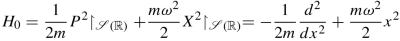
  where P := P ₁ in the notation of Example (2), $D(H_0) := {\mathcal {S}}({\mathbb R})$ (evidently), and both $\frac {d}{dx}$ and the multiplication by x ² act on $\mathcal {S}({\mathbb R})$.

  We claim H ₀ is essentially selfadjoint. It is convenient to define operators $A,A^\dagger , \mathcal {N} : \mathcal {S}({\mathbb R}) \to L^2({\mathbb R},dx)$ by

  

  (2.26)

  These operators have common domain ${\mathcal {S}}({\mathbb R})$ which is also invariant:

  $$\displaystyle \begin{aligned}A(\mathcal{S}({\mathbb R})) \subset \mathcal{S}({\mathbb R})\:, \:\: A^\dagger(\mathcal{S}({\mathbb R})) \subset \mathcal{S}({\mathbb R})\:, \:\: \mathcal{N}(\mathcal{S}({\mathbb R})) \subset \mathcal{S}({\mathbb R})\:.\end{aligned}$$

  Applying Definition 2.23 to the first two objects in (2.26) and integrating by parts gives $A^\dagger \subsetneq A^*$ and $A \subsetneq (A^\dagger )^*$. The inclusion is strict because D(A ^∗) and D((A ^†)^∗) also contain, for instance, C ¹ maps with compact support which do not belong to $\mathcal {S}({\mathbb R})$. The operator $\mathcal {N}$ is Hermitian and symmetric because $\mathcal {S}({\mathbb R})$ is dense in $L^2({\mathbb R}, dx)$. By direct computation

  $$\displaystyle \begin{aligned}H_0 = \hbar \left(A^\dagger A + \frac{1}{2}I\right) = \hbar \left(\mathcal{N} + \frac{1}{2}I\right)\:.\end{aligned}$$

  We have the commutation relation

  $$\displaystyle \begin{aligned} \begin{array}{rcl} [A, A^\dagger] = I_{\mathcal{S}({\mathbb R})}\:{} \end{array} \end{aligned} $$

  (2.27)

  (both sides are viewed as operators $\mathcal {S}({\mathbb R})\to \mathcal {S}({\mathbb R})$). Let us suppose that there exists $\psi _0 \in \mathcal {S}({\mathbb R})$ such that

  $$\displaystyle \begin{aligned} \begin{array}{rcl} ||\psi_0|| = 1\:, \quad A \psi_0 = 0{}\:. \end{array} \end{aligned} $$

  (2.28)

  Starting from (2.27) and using an inductive procedure on the vectors

  $$\displaystyle \begin{aligned} \begin{array}{rcl} \psi_n := \frac{1}{\sqrt{n!}} (A^\dagger)^n \psi_0\in \mathcal{S}({\mathbb R})\:,{} \end{array} \end{aligned} $$

  (2.29)

  it is easy to prove that (e.g., see [SaTu94, Mor18] for elementary details)

  $$\displaystyle \begin{aligned} \begin{array}{rcl} A \psi_n = \sqrt{n} \psi_{n-1}\:, \quad A^\dagger \psi_n = \sqrt{n+1} \psi_{n+1}\:, \quad \langle \psi_n|\psi_m\rangle = \delta_{nm}\:{}\end{array} \end{aligned} $$

  (2.30)

  for n, m = 0, 1, 2, …. Finally, the ψ _n are eigenvectors of H ₀ (and $\mathcal {N}$) since

  $$\displaystyle \begin{aligned} \begin{array}{rcl} H_0 \psi_n = \hbar \omega \left(A^\dagger A\psi_n + \frac{1}{2}\psi_n\right) = \hbar \omega \left(A^\dagger \sqrt{n} \psi_{n-1} + \frac{1}{2}\psi_n\right) =\hbar \omega\left(n + \frac{1}{2}\right) \psi_n\:.\qquad \end{array} \end{aligned} $$

  (2.31)

  As a consequence, if we can find ψ ₀, $\{\psi _n\}_{n\in {\mathbb N}}$ is an orthonormal set. It actually is a Hilbert basis called the Hilbert basis of Hermite functions. To prove it, by Definition 2.10 it suffices to demonstrate that the span of the ψ _n has trivial orthogonal complement:

  $$\displaystyle \begin{aligned}\mbox{if}\ f\in L^2({\mathbb R}, dx),\quad \int_{\mathbb R} f(x) \psi_n(x) dx =0\quad \mbox{for every}\ n\in {\mathbb N}\ \mbox{implies}\ f=0.\end{aligned}$$

  To this end, observe that (2.28) admits a unique solution in $\mathcal {S}({\mathbb R})$ up to constant unit factors, namely

  $$\displaystyle \begin{aligned}\psi_0(x) = \frac{1}{\pi^{1/4}\sqrt{s}}e^{-\frac{x^2}{2s^2}}\:, \quad s:= \sqrt{\frac{\hbar}{m\omega}}\:.\end{aligned}$$

  From (2.29), by rescaling the argument of ψ _n,

  $$\displaystyle \begin{aligned}\psi_n(x) = \sqrt{s}H_n(x/s)\:,\quad H_n(x):= \frac{1}{\sqrt{2^n \pi^{1/2} n!}}\left(x - \frac{d}{dx}\right)^n e^{-x^2/2}\:,\quad n=0,1,\ldots\:. \end{aligned}$$

  In particular $\psi _n \in \mathcal {S}({\mathbb R})$. Furthermore, since $H_n(x) e^{+\frac {x^2}{2}}$ is a polynomial of degree n, the condition $\int _{\mathbb R} f \psi _n dx =0$ for every $n\in {\mathbb N}$ implies by induction

  $$\displaystyle \begin{aligned}\int_{\mathbb R} f(x) x^n e^{-x^2/2} dx =0 \quad \mbox{ for every}\ n\in {\mathbb N}.\end{aligned}$$

  (Notice that the integrand is a product of L ² functions, and hence is L ¹). Hence, $\forall k\in {\mathbb R}$,

  $$\displaystyle \begin{aligned}\begin{aligned}\int_{{\mathbb R}}\hskip -3pt e^{-ikx}f(x) e^{-\frac{x^2}{2}} dx &= \hskip -3pt \int_{{\mathbb R}} \hskip -3pt \lim_{N\to+ \infty}\sum_{n=0}^{N}\frac{(-ik)^n}{n!} x^n f(x) e^{-\frac{x^2}{2}} dx\\ &= \hskip -3pt \lim_{N\to+ \infty}\hskip -3pt \sum_{n=0}^{N}\frac{(-ik)^n}{n!} \hskip -3pt \int_{{\mathbb R}}\hskip -3pt f(x) x^n e^{-\frac{x^2}{2}} dx =0\:.\end{aligned}\end{aligned}$$

  Integral and sum can be exchanged by dominated convergence, since

  $$\displaystyle \begin{aligned}\begin{aligned}\left|\sum_{n=0}^{N}\frac{(-ik)^n}{n!} x^n f(x) e^{-\frac{x^2}{2}}\right| &\leq \sum_{n=0}^{N}\frac{|k|{}^n}{n!} |x|{}^n |f(x)| e^{-\frac{x^2}{2}}\\ &= \sum_{n=0}^{+\infty}\frac{|k|{}^n}{n!} |x|{}^n |f(x)| e^{-\frac{x^2}{2}}= e^{|kx|-\frac{x^2}{2}} |f(x)| \end{aligned}\end{aligned}$$

  and the function ${\mathbb R} \ni x \mapsto e^{|kx|-\frac {x^2}{2}} |f(x)|$ is L ¹.

  We have shown that the L ¹-Fourier transform of ${\mathbb R} \ni x \mapsto f(x) e^{-x^2/2}$ vanishes everywhere. Since the L ¹-Fourier transform is linear and injective (see Remark 2.45), $f(x) e^{-x^2/2}=0$ a.e., and hence f = 0 in L ² as we wanted. We have established that the set of eigenvectors $\{\psi _n\}_{n \in {\mathbb N}}\subset \mathcal {S}({\mathbb R})$ of H ₀ is a Hilbert basis of $L^2({\mathbb R}, dx)$, as promised.

  Using Nelson’s criterion the symmetric operator H ₀ is essentially selfadjoint in $D(H_0) = \mathcal {S}({\mathbb R})$, because H ₀ admits a Hilbert basis of eigenvectors with corresponding eigenvalues $\hbar \omega (n + \frac {1}{2})$. It is worth stressing that, physically speaking, the Hamiltonian operator of the harmonic oscillator is the selfadjoint operator $H:= \overline {H_0} = H_0^*$. This is however completely determined by the non-selfadjoint operator H ₀.

• (5) Assume as usual ħ = 1. The operator

  $$\displaystyle \begin{aligned}P':= -i\frac{d}{dx} \quad \mbox{acting on}\quad f\in D(P') := \{ f \in C^2([0,1])\:|\: \mbox{supp}(f) \subset (0,1)\}\end{aligned}$$

  is sometimes called, improperly, momentum operator in a box. (Evidently at 0 and 1 only the right and the left derivatives are considered, and with little effort one may define it on [a, b] instead of [0, 1]). D(P′) is dense in L ²([0, 1], dx) and it is easy to prove that P′ is symmetric using integration by parts. Moreover P′ commutes with the conjugation $(C\psi )(x) := \overline {\psi \left (\frac {1}{2}-x\right )}$, so it admits selfadjoint extensions (n ₊ = n ₋) by Proposition 2.50. It is easy to see that n _±≥ 1 because χ _±(x) := e ^±x satisfies 〈χ _±|P′f〉 = ±i〈χ _±|f〉 for every f ∈ D(P′), which means P′ ^∗ χ _± = ±iχ _±. Actually a closer scrutiny (exercise!) shows that n _± = 1. In any case, Proposition 2.47 tells P′ is not essentially selfadjoint because n _± > 0. It is possible to find various selfadjoint extensions of P′ (the only ones admitted, by Theorem 2.48) as we proceed to illustrate. For $\alpha \in {\mathbb R}$, extend P′ to

  $$\displaystyle \begin{aligned} \begin{array}{rcl} P^{\prime}_\alpha f := -i\frac{df}{dx} \quad \mbox{for}\quad f \in D(P^{\prime}_\alpha) := \{ f \in C^2([0,1])\:|\: f(1) = e^{i\alpha}f(0)\}\\{}\end{array} \end{aligned} $$

  (2.32)

  and observe that $D(P^{\prime }_\alpha )=D(P^{\prime }_{\alpha '})$ if α′ = α + 2kπ, $k\in {\mathbb Z}$, so that we can restrict α to [0, 2π). By direct inspection, it is also evident that $P^{\prime }_\alpha \subset {P^{\prime }_\alpha }^*$, i.e., $P^{\prime }_\alpha$ is symmetric: boundary terms cancel out in the inner product and $\langle f|P^{\prime }_\alpha g\rangle = \langle P^{\prime }_\alpha f| g\rangle$ if $f,g \in D(P^{\prime }_\alpha )$. Actually $P^{\prime }_\alpha$ is essentially selfadjoint because it admits the Hilbert basis of eigenvectors

  $$\displaystyle \begin{aligned}u_{\alpha,n}(x) := e^{i2\pi(\alpha + n)x}\:,\quad n\in {\mathbb Z}\:.\end{aligned}$$

  That is indeed a Hilbert basis because u _α,n = U _α u _0,n where (U _α ψ)(x) := e ^iαx ψ(x), ψ ∈ L ²([0, 1], dx), defines a unitary operator, and u _0,n(x) = e ^i2πnx, $n\in {\mathbb Z}$, is a well-known Hilbert basis of L ²([0, 1], dx). Thus we have found a family of selfadjoint extensions of P′ labelled by α ∈ [0, 2π): $P_\alpha := \overline {P^{\prime }_\alpha } = {P^{\prime }_\alpha }^*$. If α, α′∈ [0, 2π) and α ≠ α′, then $P_\alpha \neq P_{\alpha '}$ since the eigenvalues are different: α + 2nπ and and α′ + 2nπ ($n \in {\mathbb Z}$) respectively. These selfadjoint extensions were constructed just by specializing the boundary conditions defining the domain of the original symmetric operator P′ according to (2.32). Using Theorem 2.48 and Remark 2.49 (a) it is easy to prove that (exercise!) P′ has no further selfadjoint extensions (i.e., other than the P _α, α ∈ [0, π)) [ReSi80, Tes14, Mor18]. In contrast to what happens for the momentum operator defined on the entire $L^2({\mathbb R},dx)$, P _α does not leave invariant its core $D(P^{\prime }_\alpha )$ (think of the core $\mathcal {S}({\mathbb R})$, which is invariant under the action of the momentum operator on $L^2({\mathbb R},dx)$). Given these domain issues, P _α fails in particular the Heisenberg commutation relations relatively to the natural definition of the selfadjoint position operator X,

  $$\displaystyle \begin{aligned}(Xf)(x) = xf(x)\quad \mbox{for}\quad f\in D(X) := \left\{f \in L^2([0,1],dx)\:\left|\: \int_0^1 |xf(x)|{}^2 dx\right. <+\infty\right\}\:,\end{aligned}$$

  restricted to the common core $D(P^{\prime }_\alpha )$. In fact, this space is a core for X as well but, again, it is not invariant under it: in general P _α Xf will not make sense if $f\in D(P^{\prime }_\alpha )$, so [X, P _α] cannot be computed on D(P _α), in contrast to the position and momentum operators on ${\mathbb R}$ and referring to the common core $\mathcal {S}({\mathbb R})$. $\blacksquare$

References

V. Moretti, Spectral Theory and Quantum Mechanics, 2nd edn. (Springer, Cham, 2018)
J. von Neumann, Mathematische Grundlagen der Quantenmechanik (Springer, Berlin, 1932)
G.K. Pedersen, Analysis Now. Graduate Texts in Mathematics, vol. 118 (Springer, New York, 1989)
M. Reed, B. Simon, Methods of Modern Mathematical Physics II: Fourier Analysis, Self-Adjointness (Academic, New York, 1975)
M. Reed, B. Simon, Methods of Modern Mathematical Physics I: Functional Analysis. Revised and Enlarged Edition (Academic, New York, 1980)
W. Rudin, Functional Analysis, reprinted edition (Dover, Mineola, 1990)
J.J. Sakurai, S.F. Tuan, Modern Quantum Mechanics, revised edition (Pearson Education, Delhi, 1994)
K. Schmüdgen, Unbounded Self-Adjoint Operators on Hilbert Space (Springer, Dordrecht, 2012)
B. Simon, The theorem of semi-analytic vectors: a new proof of a theorem of Masson and McClary. Indiana Univ. Math. J. 20(12), 1145–1151 (1971)
G. Teschl, Mathematical Methods in Quantum Mechanics with Applications to Schrödinger Operators. Graduate Studies in Mathematics, 2nd edn. (AMS, Providence, 2014)
Author information
Authors and Affiliations
Rights and permissions
Copyright information
© 2019 Springer Nature Switzerland AG
About this chapter
Cite this chapter
Moretti, V. (2019). Hilbert Spaces and Classes of Operators. In: Fundamental Mathematical Structures of Quantum Theory. Springer, Cham. https://doi.org/10.1007/978-3-030-18346-2_2
Download citation
DOI: https://doi.org/10.1007/978-3-030-18346-2_2
Published:
Publisher Name: Springer, Cham
Print ISBN: 978-3-030-18345-5
Online ISBN: 978-3-030-18346-2
eBook Packages: Physics and AstronomyPhysics and Astronomy (R0)