Applications to Plasma Spectroscopy

Abstract

Applications to plasma spectroscopy are presented for different types of plasmas that are currently of great interest for science and applications: low-density tokamak plasmas, dense optical laser-produced plasmas, high-current Z-pinch plasmas, and X-ray Free Electron Lasers interacting with solids. The general principles of plasma electron temperature and density measurements as well as the characterization of suprathermal (hot electrons) and non-equilibrium phenomena are presented. Particular attention is based on the innovative concepts of dielectronic satellite and hollow ion X-ray emission. The effect of a neutral background that is coupled to plasma ions via charge exchange is considered in the framework of nonlinear atomic kinetics. Transient phenomena in the start-up phase, impurity diffusion, sawtooth oscillations, and superthermal electrons are discussed for magnetic fusion plasmas. For dense laser-produced plasmas and charge exchange coupling of colliding plasmas, the dynamics of fast ions in space and energy distribution functions are presented. The interaction of XFEL with solids is considered in the framework of a new kinetic plasma theory, where generalized atomic processes provide a link from the cold solid until the hot diluted plasma. Three-body recombination and Auger electrons constitute a generalized three-body recombination that is identified to play also a new role as a direct heating mechanism. General principles and new theories are illustrated along with detailed comparisons with experimental data.

10.1 The Emission of Light and Plasma Spectroscopy

The emission of light is one of the most fascinating phenomena in nature. Everybody feels the beauty while looking at the colors appearing at sunset, when a bolt of lightning illuminates the night, or when the emission of the aurora moves like magic in the dark heaven. And every day, we are looking at something in order to read information from a computer screen, to drive not into but around an obstacle, to look into the eyes of the child to understand that it tries to hide that it just burned off fathers’ stamp collection in an unlucky physical experiment.

In general terms, we all use light to obtain information, to diagnose something, to control or optimize a process, or to understand what is true and what is right. And since the discovery of the spectral analysis, no one doubted that the problems of describing atoms and matter would be solved once we had learned to understand the language of atomic spectra and the emission of light.

Light also transports energy, and it is the flow of energy from sunlight that has so much impacted on the evolution of our blue planet.

The “Radiative properties of Matter” is the related basic science, and their analysis for diagnostic purposes is called “Spectroscopy”. Questions like “Why the heaven is blue?”, “What is the temperature in the flame of a candle?”, and “What makes the sun burning so wonderful?” have been the historical origin of scientific activity. We also might ask what light is by itself? This is a difficult question: Although almost everybody has some imagination what light is, it is difficult to say what it really is.

The light emission is accompanied by the transport of energy and the well-known formula

$$E_{\omega } = \hbar \omega$$

(10.1)

(where $\hbar$ is the Planck constant and $\omega$ the photon angular frequency) that manifests in a scientific manner the double role of light: the beauty of photons when looking at their various colors and the energy that is carried by them with their own velocity – the speed of light c.

That any radiating source loses consequently energy via its own radiation has a large impact on the evolution of the system itself. In general terms, the radiation losses influence on the energy balance of the system that is coupled to the motion of the particles from which the system is composed.

An impressive example of the importance of radiation losses is known from the early days of the fusion research based on the magnetic confinement invented in the 50s by the two Russians Igor Tamm and Andrei Sakharov: The term tokamak was likewise created by the Russians: “тopoидaльнaя кaмepa c мaгнитными кaтyшкaми” (toroïdalnaïa kamera s magnitnymi katushkami = toroidal chamber with magnetic coils). The radiation emission from the impurities in the tokamak had been so large that it overcompensated the energy input leading to a plasma disruption. Only after generations of very intense and successful material research, the number of impurity atoms and ions could drastically be reduced to maintain tokamak discharges for more than minutes. A milestone in the tokamak research can be attributed to the year 1969: The Kurchatov Institute in Russia, Moscow, has announced to have obtained a tokamak discharge with an electron temperature of kT_e > 1 keV (means that the level of the right order of magnitude was reached where fusion reactions become probable). The scientific western community did not believe these results, and in 1969, an experimental group from England went to the Kurchatov Institute to measure independently the electron temperature with Thomson scattering. This group could only confirm the results announced by the Russians, and in the following years, many countries followed the Russian way of magnetic fusion research building many tokamaks all over the world.

Plasma radiation plays likewise an important role in the inertial confinement fusion (ICF). Here, fusion of the DT capsule is envisaged by means of powerful laser installations like NIF, MEGAJOULE, and GEKKO. In the indirect drive, the radiation field in the hohlraum (initiated by megajoule laser irradiation of the inner surface of the hohlraum composed of an heavy element like gold) is supposed to deliver energy to the capsule to evaporate in a homogenous manner (assuming that the hohlraum radiation is very close to the blackbody radiation) the ablator surface that in turn compresses the fusion material to ignition relevant parameters. In the direct drive approach, laser radiation is directly interacting with the capsule. Today, many other schemes of compression are investigated like fast ignition or shock ignition.

In astrophysics, radiation phenomena are strongly connected with the energy transport in stars from the fusion source in the inner part of the star to its surface. Therefore, so-called radiation transport plays an important role in star evolution.

Today, the study of the radiative properties of matter has proven to be one of the most powerful methods to understand various physical phenomena. Plasma spectroscopy (Griem 1964, 1974, 1997; McWhirter 1965; Lochte-Holtgreven 1968; Michelis and Mattioli 1981; Boiko et al. 1985; Lisitsa 1994; Fujimoto 2004; Sobelman and Vainshtein 2006; Kunze 2009, Rosmej 2012a) provides essential information about basic parameters, like temperature, density, chemical composition, velocities, and relevant physical processes (“Why the aurora is green at low altitudes but red at larger ones?”, “Why can we look with X-rays into the human body but not with visible light ?”,…).

The accessible parameter range of spectroscopy covers orders of magnitude in temperature and (especially) density, because practically all elements of particular, selected isoelectronic sequences can be used for diagnostic investigations. These elements can occur as intrinsic impurities or may be intentionally injected in small amounts (so-called tracer elements). This makes plasma spectroscopy also a very interdisciplinary science.

The rapid development of powerful laser installations including X-ray Free Electron Lasers, intense heavy ion beams, and the fusion research (magnetic and inertial fusion) enable the creation of matter under extreme conditions never achieved in laboratories so far. An important feature of these extreme conditions is the non-equilibrium nature of the matter, e.g., a solid is heated by a fs-laser pulse and undergoes a transformation from a cold solid to warm dense matter to strongly coupled plasma and then to a highly ionized gas while time is elapsing. We might think about using time-dependent detectors to temporally resolve the light emission in the hope to have then resolved the problem. However, this is not so simple: There are not only serious technical obstacles but also basic physical principals to respect. A simple technical reason is that for 10 fs-laser radiation interacting with matter, we do not have any X-ray streak camera available (the current technical limit is about 0.5 ps). A simple principal reason is that the atomic system from which light originates has a characteristic time constant (see also Sect. 6.2) that might be much longer than 10 fs. The atomic system is therefore “shocked,” and any light emission is highly out of equilibrium even if the experimental observation is time resolved. Note, that only recently general studies of shocked atomic systems have begun (Deschaud et al. 2020).

In high-energy-density physics, laser-produced plasmas, and fusion research, the light emission in the X-ray spectral range is of particular interest: Only the X-ray emission is in general able to exit the volume without essential photoabsorption. Therefore, X-ray plasma spectroscopy is of particular interest to obtain information from objects that are not well understood or to control certain processes that are useful for applications (Renner and Rosmej 2019).

We are therefore looking to develop X-ray radiative properties and the related atomic and plasma physics to study non-equilibrium states of matter. This is a challenging field of activity for research and applications: Non-equilibrium atomic kinetics (see Chap. 6) involve fascinating topics in atomic physics of dense plasmas, like the study of exotic dense states of matter (like hollow ions and hollow crystals) with XFEL (Rosmej 2012a, b; Deschaud et al. 2020), the discovery by high-resolution spectroscopy of a new heating mechanism like Auger electron heating (Galtier et al. 2011; Rosmej 2012b; Petitdemange and Rosmej 2013), and three-body recombination assisted heating (Deschaud et al. 2014), see also Sect. 10.6.4.6. Radiative properties have likewise strong links and important impact to magnetic confinement fusion (MCF), inertial confinement fusion (ICF), and particular X-ray spectroscopy, and related atomic physics is a key element to study matter irradiated by X-ray Free Electron X-ray Lasers (XFEL).

It is often not quite clear what is meant with the word “Equilibrium.” Does this mean that the plasma parameters do not change in time, which means for a parameter X:

$$\partial X/\partial t = 0$$

(10.2)

or does the word “Equilibrium” mean that the particle statistics follows certain laws? Or something else?

In thermodynamics (Huang 1963; Reif 1965; Alonso and Finn 1968), the “Equilibrium” of an isolated system is characterized by the maximum entropy¹:

$$\delta S = \delta \left\{ {k\,\ln \,W} \right\} = 0.$$

(10.3)

k is the Boltzmann constant, and W is the microscopic probability (probability means “Wahrscheinlichkeit” in german) of a certain configuration which means the probability P(N, N₁, N₂ … N_M) to distribute N particles over M states with respective populations N₁, N₂ … N_M.

It is important to realize that conditions (10.2) and (10.3) are entirely different: Thermodynamic equilibrium is not determined by ∂/∂t = 0. In other words, the Saha–Boltzmann equation, the Planck radiation, the Maxwellian energy distribution function of free electrons,… are consequences of (10.3), and these laws cannot be obtained from (10.2). These laws are the solution of (10.3) for different particle statistics.

In most cases, laws obtained from (10.3) concern isolated systems, which means that external forces do not play a role for the particle statistics. What does it mean that external forces do not play an important role? In atomic physics, this means that external forces have to be compared with the “Atomic Forces.” Let us consider an example to illustrate this: the interaction of a high-intensity laser with a plasma. The external force is the laser electric field E_laser:

$$I_{\text{laser}} = c \varepsilon_{0} \left\langle {E_{\text{laser}}^{2} } \right\rangle.$$

(10.4)

I_laser is the laser intensity, c the speed of light, and ε₀ the electrical permittivity. Rewriting (10.4) in convenient units, we obtain:

$${E}_{\rm{laser}} \approx \sqrt {\left\langle {{E}^{2} } \right\rangle} = \sqrt {\displaystyle\frac{I}{{{c} {\varepsilon}_{0} }}} = 19.4 \sqrt {{I}\left( {\displaystyle\frac{{W}}{{cm}^{2}} }\right)} \left[ {\displaystyle\frac{\rm{V}}{\rm{cm}}} \right].$$

(10.5)

The relevant forces for an ion in a plasma are the atomic ones. They can be estimated with the simple Bohr atomic model:

$$E_{\rm{Atom}} \approx \displaystyle\frac{1}{{4\pi \varepsilon_{0}}} \displaystyle\frac{{Z \cdot {e}}}{{\left( {a_{0} n^{2} /Z} \right)^{2} }} = \displaystyle\frac{e}{{4\pi \varepsilon_{0} a_{0}^{2}}} \displaystyle\frac{{Z^{3} }}{{n^{4} }}$$

(10.6)

or, expressed in convenient units

$$E_{\rm{Atom}} \approx 5.14 \times 10^{9} \displaystyle\frac{{Z^{3}}}{{n^{4}}} \,\left[ {\displaystyle\frac{\rm{V}}{\rm{cm}}} \right].$$

(10.7)

The standard atomic field, i.e., E_a.u. = 5.14 × 10⁹ V/cm (see also Annex A.5) is therefore obtained for a laser intensity of I_a.u. = 7.0 × 10¹⁶ W/cm². This means, e.g., that the 1s level of atomic hydrogen is weakly perturbed for laser intensities being many orders of magnitudes lower than I_a.u..

Let us now consider the influence of the electrical laser field on the radiative properties of atoms and ions in a plasma. Due to the interaction of the laser electric field with the free electrons in the plasma, suprathermal electrons (or hot electrons) are generated. They seriously alter the light emission. First, there is an enhanced ionization due to hot electrons because ionization is more effective. The second change concerns the qualitative distortion of ionic charge stage distribution (Rosmej 1997). The visualization of the distortion of the charge stage distribution by high-resolution X-ray spectroscopy has been applied to inertial fusion hohlraums to determine the time-dependent hot electron fraction and the relevant mechanism of hot electron generation (Glenzer et al. 1998). Let us define the suprathermal electron fraction according to:

$$f_{\text{hot}} = \displaystyle\frac{{n_{\text{e}} \left( {{hot}} \right)}}{{n_{\text{e}} \left( {{bulk}} \right) + n_{\text{e}} \left( {{hot}} \right)}}.$$

(10.8)

n_e,hot is the hot electron density, n_e,bulk is the bulk electron density. n_e,hot + n_e,bulk is therefore the total electron density, and (10.8) fulfills the normalization condition. It is important to realize that even rather small amounts of hot electrons (low as of the order of 10⁻⁵) might have a considerable influence on the radiative properties, especially if the bulk electron temperature is low. This is due to the exponential temperature dependence of the excitation (C) and ionization (I) rate coefficients (see also Sects. 5.3.1 and 5.4.3), i.e.,

$$C \propto \displaystyle\frac{{\exp \left( { - \Delta E/kT_{\text{e}} } \right)}}{{\sqrt {kT_{\text{e}} } }},$$

(10.9)

$$I \propto \displaystyle\frac{{\exp \left( { - E_{\text{i}} /kT_{\text{e}} } \right)}}{{\sqrt {kT_{\text{e}} } }}.$$

(10.10)

ΔE is the excitation energy of an atomic transition, E_i is the ionization energy of a particular atomic level, and T_e is the electron temperature.

It should be realized that small fractions of hot electrons can be produced already with laser intensities of 10¹⁵ W/cm² (Gitomer et al. 1986; Beg et al. 1997) and therefore the value of the laser electric field above which an important influence on the radiative properties is expected might be well below I_a.u. = 7.0 × 10¹⁶ W/cm². We note that suprathermal electrons generated in ICF hohlraums (e.g., generated by SBS = Stimulated Brillouin Scattering) may lead to a preheat of the DT target which in turn prevents efficient compression necessary to reach ignition. Suprathermal electrons (hot electrons) are therefore a very actual problem in the laser-driven inertial fusion ignition campaigns (Lindl 1995, Lindl et al. 2004, 2014; Atzeni 2009). We note that in the more recently discussed shock ignition scheme (Betti et al. 2007), suprathermal electrons impact on the fusion performance as an important fraction of laser energy is coupled to hot electrons.

In tokamaks, much lower electric fields lead to the generation of suprathermal electrons: Due to the low electron density, the collisional drag is small and even electric field values of the order of some V/cm (the so-called Dreicer field, Wesson 2004) lead to runaway electrons: The collisional drag is insufficient to compensate the electron acceleration due to the electric field and numerous circulations in the tokamak may then lead to electron energies up to MeV. These MeV electrons seriously influence on the fusion performance (e.g., electrons accelerated by lower hybrid waves, investigation of suitable current drives). These two foregoing examples show that the importance of an external force is not specified by an absolute value but rather by the comparison of the external force with the relevant “internal” one.

Let us now consider the principle idea for spectroscopic diagnostics that is based on line intensity ratios. Having once calculated the non-LTE level populations according to (6.22), all combinations of line intensity ratios can be obtained:

$$\displaystyle\frac{{I_{\text{ji}} }}{{I_{{\text{j}^{\prime } \text{i}^{\prime } }} }} = \displaystyle\frac{{\omega_{\text{ji}} }}{{\omega_{{\text{j}^{\prime } \text{i}^{\prime } }} }} \displaystyle\frac{{A_{\text{ji}} }}{{A_{{\text{j}^{\prime } \text{i}^{\prime } }} }} \displaystyle\frac{{n_{\text{j}} }}{{n_{{\text{j}^{\prime } }} }}.$$

(10.11)

Of particular interest are those intensity ratios that depend only on one plasma parameter. The ideal case of a temperature diagnostic is therefore given by

$$\displaystyle\frac{{I_{\text{ji}} }}{{I_{{\text{j}^{\prime } \text{i}^{\prime } }} }} = G_{{\text{jij}^{\prime } \text{i}^{\prime } }} \left( {T_{\text{e}} } \right),$$

(10.12)

whereas the ideal case of a density diagnostic is represented by the relation

$$\displaystyle\frac{{I_{\text{kl}} }}{{I_{{\text{k}^{\prime } \text{l}^{\prime } }} }} = \gamma_{{\text{klk}^{\prime } \text{l}^{\prime } }} \left( {n_{\text{e}} } \right).$$

(10.13)

The functions G and γ are obtained from the solution of the system of rate equations (6.22). Having measured these intensity ratios with appropriate line emissions, the application of (10.12), (10.13) provides readily temperature and density. However, the solution of (6.22) shows that in general, the intensity ratio depends both on temperature and density:

$$\displaystyle\frac{{I_{\text{ji}} }}{{I_{{\text{j}^{\prime } \text{i}^{\prime } }} }} = \chi_{{\text{jij}^{\prime } \text{i}^{\prime } }} \left( {T_{\text{e}} ,n_{\text{e}} } \right).$$

(10.14)

One aim of spectroscopic research is to find line ratios whose dependence is close to those of the ideal (10.12), (10.13). The difficulty in doing so lies in the fact that (10.14) has multiple solutions, which means that for different sets of density and temperature the same line intensity ratio is obtained (note that the two-parameter dependence is a simplified case and opacity, hot electrons and transient plasma evolution might considerably increase the complexity). It is therefore necessary to employ several line ratios at the same time to avoid misleading parameter information from single line ratios.

10.2 Dielectronic Satellite Emission

10.2.1 Electron Temperature

10.2.1.1 Satellite to Resonance Lines

Gabriel has introduced the dielectronic satellite transitions (see also Chap. 5) as a sensitive method to determine the electron temperature in hot plasmas (Gabriel 1972) that is based on dielectronic capture and dielectronic recombination (see also Sect. 5.6 and review [Rosmej et al. 2020a]). In low-density plasmas, this method approaches the ideal picture of a temperature diagnostic according to (10.12). Numerical calculations show (see also Sect. 6.3.2 and following Figures 10.2 and 10.3) that also in high-density plasmas, this method is still applicable and one of the most powerful methods for electron temperature determination of hot dense plasmas.

Let us therefore consider the basic principles via an example: The dielectronic satellites 2l2l′ near the Lyman-alpha line of H-like ions (Fig. 5.1 show the relevant energy level diagram). As the He-like states 2l2l′ are located above the ionization limit, a non-radiative decay to the H-like ground state (autoionization) is possible:

$$\text{autoionization}: 2l2l^{\prime } \to 1s + e.$$

(10.15)

By first quantum mechanical principles, the reverse process, so-called dielectronic capture, must exist:

$$\text{dielectronic}\,\text{capture}: 1s + e \to 2l2l^{\prime }.$$

(10.16)

The radiative decay reads

$$\text{radiative}\,\text{decay}: 2l2l^{{\prime }} \to 1s2l + \hbar \omega_{\text{satellite}}.$$

(10.17)

The emitted photon is called a “satellite.” The satellite transition is of similar nature like the resonance transition ${Lyman}_{\alpha } = 2p \to 1s + \hbar \omega_{{{Ly}_{\alpha } }}$ except the circumstance that an additional electron is present in the quantum shell n = 2, the so-called spectator electron. As the spectator electron screens the nuclear charge, the satellite transitions are essentially located on the long wavelength side of the corresponding resonance line. However, due to intermediate coupling effects and configuration interaction, also satellites on the short wavelengths side are emitted (see Fig. 10.1), so-called blue satellites (Rosmej and Abdallah 1998).

As the number of possible angular momentum couplings increases rapidly with the number of electrons, usually numerous satellite transitions are located near the resonance line (which often cannot be resolved spectrally even with high-resolution methods). Figure 10.1 shows an example of the Lyman_α satellite transitions obtained in a dense laser-produced magnesium plasma. The experiment shows also higher-order satellites where the spectator electrons are located in quantum shells n > 2 (configurations 2lnl′).

Fig. 10.1

Dielectronic satellite emission near Lyman-alpha of H-like Mg ions in a dense laser-produced plasma (50 J, 15 ns, 1.064 μm). Spectral simulation of optically thick plasma has been carried out with the MARIA code for an electron temperature of kT_e = 210 eV, electron density of n_e = 3 × 10²⁰ cm⁻³, effective photon path length L_eff = 500 μm, inhomogeneity parameter s = 1.3

Let us now proceed to the genius idea of Gabriel to obtain the electron temperature from satellite transitions. In a low-density plasma, the intensity of the resonance line is given by

$$I_{{\text{k}^{{\prime }} ,\text{j}^{{\prime }} \text{i}^{{\prime }} }}^{\text{res}} = n_{\text{e}} n_{{\text{k}^{{\prime }} }} \displaystyle\frac{{A_{{\text{j}^{{\prime }} \text{i}^{{\prime }} }} }}{{\sum\nolimits_{{\text{l}^{{\prime }} }} {A_{{\text{j}^{{\prime }} \text{l}^{{\prime }} }} } }} \left\langle {C_{{\text{k}^{{\prime }} \text{j}^{{\prime }} }} } \right\rangle,$$

(10.18)

where n_e is the free electron density, n_k′ the ground state density from which electron collisional excitation proceeds (k′ is the 1s level in our example), A_j′i′ is the transition probability of the resonance transition j′→ i′ (the sum over A in the denominator accounts for possible branching ratio effects), and $\left\langle {C_{{\text{k}^{{\prime }} \text{j}^{{\prime }} }} } \right\rangle$ is the electron collisional excitation rate coefficient from level k′ to level  j′. The intensity of a satellite transition with a large autoionizing rate (and negligible collisional channel) is given by

$$I_{\text{k,ji}}^{\text{sat}} = n_{\text{e}} n_{\text{k}} \displaystyle\frac{{A_{\text{ji}} }}{{\sum\nolimits_{l} {A_{\text{jl}} + \sum\nolimits_{m} {\Gamma _{\text{jm}} } } }} \left\langle {D_{\text{kj}} } \right\rangle.$$

(10.19)

A_ji is the transition probability of the particular satellite transition, and $\left\langle {D_{\text{kj}} } \right\rangle$ is the dielectronic capture rate coefficient from level k to the level j. The sums over the radiative decay rates and autoionizing rates account for possible branching ratio effects (in our simple example, only m = k exist, a particular upper-level 2l2l′ may have more than one radiative decay possibilities j → l). We note that already for the He_β satellites, numerous autoionizing channels exist which are very important in dense plasmas (Rosmej et al. 1998). As both intensities of (10.18), (10.19) are proportional to the electron density n_e and to the same ground state density (k′ = k), the intensity ratio is a function of the electron temperature only, because the rate coefficients $\left\langle C \right\rangle$ and $\left\langle D \right\rangle$ depend only on the electron temperature but not on the density:

$$\displaystyle\frac{{I_{\text{k,ji}}^{\text{sat}} }}{{I_{{\text{k}^{{\prime }} \text{j}^{{\prime }} \text{i}^{{\prime }} }}^{\text{res}} }} = G\left( {T_{\text{e}} } \right).$$

(10.20)

The dielectronic capture rate (see also Chap. 5) is an analytical function and given by

$$\left\langle {D_{\text{kj}} } \right\rangle = \alpha\Gamma_{\text{jk}} \displaystyle\frac{{g_{\text{j}} }}{{g_{\text{k}} }}\displaystyle\frac{{\exp \left( { - E_{\text{kj}} /kT_{\text{e}} } \right)}}{{\left( {kT_{\text{e}} } \right)^{3/2} }}.$$

(10.21)

α = 1.6564 × 10⁻²² cm³ s⁻¹, g_j and g_k are the statistical weights of the states j and k, Γ_jk is the autoionizing rate in [s⁻¹], E_kj is the dielectronic capture energy in [eV] (see also Fig. 5.1), and kT_e is the electron temperature [eV]. The intensity of a satellite transition can therefore be written as

$$I_{\text{k,ji}}^{\text{sat}} = \alpha n_{\text{e}} n_{\text{k}} \displaystyle\frac{{Q_{\text{k,ji}} }}{{g_{\text{k}} }} \displaystyle\frac{{\exp \left( { - E_{\text{kj}} /kT_{\text{e}} } \right)}}{{\left( {kT_{\text{e}} } \right)^{3/2} }}.$$

(10.22)

Q_k,ji is the so-called dielectronic satellite intensity factor and given by

$$Q_{\text{k,ji}} = \displaystyle\frac{{g_{\text{j}} A_{\text{ji}}\Gamma _{\text{jk}} }}{{\sum\nolimits_{\text{l}} {A_{\text{jl}} + \sum\nolimits_{m} {\Gamma_{\text{jm}} } } }}.$$

(10.23)

The calculation of the dielectronic satellite intensity factors Q_k,ji requests rather complicated multiconfiguration relativistic atomic structure calculations which have to include intermediate coupling effects as well as configuration interaction.

For the ease of applications, we provide an analytical set of all necessary formulas for the most important cases to apply the temperature diagnostic via dielectronic satellite transitions near Ly_α and He_α of highly charged ions. For the dielectronic satellite intensity factor, the following formula can be employed:

$$Q = 10^{10}\, \text{s}^{ - 1} \displaystyle\frac{{C_{1} \left( {Z_{\text{n}} - C_{2} } \right)}}{{C_{3} Z_{\text{n}}^{{C_{4} }} + 1}}^{4}.$$

(10.24)

Table 10.1 provides the fitting parameters for the J-satellite near Ly_α as well as for the k-satellite and the j-satellite near He_α for all elements with nuclear charge 6 < Z_n < 30. We note that the k- and j-satellites are treated separately, as line overlapping may request their separate analysis. Note that g_k = 2 for the Ly_α-satellites and g_k = 1 for the He_α-satellites in (10.22). The dielectronic capture energies can be approximated by

Table 10.1 Z_n-scaled fitting parameters of dielectronic satellite intensity factors Q according to (10.24), the range of validity is 6 < Z_n < 30

$$E_{\text{kj}} \approx \delta \left( {Z_{\text{n}} + \sigma } \right)^{2} {Ry}.$$

(10.25)

For the Ly_α-satellites 2l2l′, δ = 0.5, σ ≈ 0.5, for the He_α-satellites 1s2l2l′, δ = 0.5, σ ≈ 0.1, and Ry = 13.6 eV. The electron collisional excitation rate coefficients have been calculated with the Coulomb–Born exchange method including intermediate coupling effects and effective potentials (using Vainshtein’s ATOM code (Vainshtein and Shevelko 1986; Sobelman and Vainshtein 2006)) and fitted into a simple Z- and β-scaled expression:

$$\left\langle {C,T_{\text{e}} } \right\rangle \approx \displaystyle\frac{{10^{ - 8} \,\text{cm}^{3}\, \text{s}^{ - 1} }}{{Z^{3} }} \left( {\displaystyle\frac{{E_{\text{u}} }}{{E_{\text{l}} }}} \right)^{3/2} \sqrt \beta\, A\,\displaystyle\frac{\beta + 1 + D}{\beta + \chi } \exp \left\{ { - \left( {E_{\text{l}} - E_{\text{u}} } \right)/kT_{\text{e}} } \right\}$$

(10.26)

with

$$\beta = \displaystyle\frac{{Z^{2} {Ry}}}{{kT_{\text{e}} }}.$$

(10.27)

Z is the spectroscopic symbol (Z = Z_n + 1 − N where Z_n is the nuclear charge and N the number of bound electrons), the fitting parameters A, χ, and D are given in Table 10.2.

Table 10.2 Fitting parameters for Z- and β-scaled electron collisional excitation rates of H-like Ly_α and He-like He_α, 1/32 < β < 32

E_l and E_u are the ionization energies of lower and upper states. If not particularly available, they can be approximated by the simple expression

$$E_{\text{j}} \approx \delta \left( {Z_{\text{n}} - \sigma } \right)^{2} {Ry}.$$

(10.28)

For the 1s-level, δ = 1, σ ≈ −0.05; for the 2p levels, δ = 0.25, σ ≈ −0.05; for the 1s² level, δ = 1, σ ≈ 0.6, and for the 1s2p ¹P₁ level, δ = 0.25, σ ≈ 1.

10.2.1.2 Rydberg Satellites

Higher-order satellites, namely 2lnl′ and 1s2lnl′, provide further possibilities for plasma diagnostics even if single transitions are not resolved. A rather tricky variant of electron temperature measurement which employs only satellite transitions has been proposed in (Renner et al. 2001):

$$\displaystyle\frac{{I_{\text{n}}^{\text{sat}} }}{{I_{2}^{\text{sat}} }} \approx \displaystyle\frac{{Q_{\text{n}} }}{{Q_{2} }} \exp \left\{ { - \displaystyle\frac{{\left( {Z_{\text{n}} - 0.6} \right)^{2} {Ry}}}{{4kT_{\text{e}} }}\left( {1 - \displaystyle\frac{4}{{n^{2} }}} \right)} \right\}.$$

(10.29)

Q_n and Q₂ are the total dielectronic satellite intensity factors for the 2lnl′ → 1snl′ and 2l2l′ → 1s2l′ transitions, respectively. The considerable advantage of this method is that it is even applicable, when the resonance line is absent due to high photoabsorption or due to very low electron temperatures—a typical situation in dense strongly coupled plasmas (Rosmej et al. 1997, 1998, 2000, 2003; Renner et al. 2001).

We note that another important excitation channel for satellite transitions is via electron collisional excitation from inner-shells. Concerning the above-discussed example of satellite transitions near Ly_α, this excitation channel reads

$$\text{inner{-}shell excitation}: 1s2l + e \to 2l2l^{\prime } + e.$$

This excitation channel is important for satellite transitions with low autoionizing rates but high radiative decay rates. It drives satellite intensities, which allow an advanced characterization of the plasma (determination of charge exchange effects in tokamaks, characterization of suprathermal electrons, to be discussed below). For electron temperature measurements, the inner-shell excitation channel should be avoided.

Figure 10.2 shows the simulations of the spectral distribution near Ly_α carried out with the MARIA code (Rosmej 1997, 1998, 2001, 2006, 2012a). Dielectronic satellites 2l2l′ as well as 2l3l′-satellites are included in the simulations for a dense plasma: n_e = 10²¹ cm⁻³. Several 2l3l′-satellites are located at the blue wavelength side of Ly_α. For these particular transitions, LS-coupling effects are as important as the screening effect originating from the spectator electron. As can be seen, numerous satellites are located at the blue wavelengths wing of the resonance line, so-called blue satellites (Rosmej and Abdallah 1998).

Fig. 10.2

MARIA simulations of the dielectronic satellite emission near Lyman-alpha of H-like Mg ions in dependence of electron temperature, n_e = 10²¹ cm⁻³

Figure 10.3 shows the MARIA simulations of the spectral distribution near He_α, dielectronic satellites 1s2l2l′, 1s2l3l′, 1s2l4l′, and 1s2l5l′ which are included in the simulations. In all cases (Figs. 10.2 and 10.3), a strong sensitivity to electron temperature is seen from dominating until vanishing dielectronic satellite contribution. The blue curve in Fig. 10.3 shows the impact of the higher-order satellite emission (n > 3) on the intensity near the resonance line Helium-alpha. It can clearly be seen that higher-order satellites may still contribute considerably to the overall line emission.

Fig. 10.3

MARIA simulations of the dielectronic satellite emission near Helium-alpha of He-like Mg ions in dependence of electron temperature, n_e = 10²¹ cm⁻³. The difference between the blue and black curve near Helium-alpha shows the impact of higher-order satellites 1s2lnl′ with n > 3

Figure 10.1 shows also the fitting of the experimental spectrum obtained in a dense laser-produced plasma experiment taking into account opacity effects (important only for the Ly_α-line). A good match to the experimental data is obtained for kT_e = 210 eV and n_e = 3 × 10²⁰ cm⁻³. The effective photon path length was L_eff = 500 μm (determined from the width of the Lyman-alpha lines as well as the intensity ratio of the Lyman-alpha components), and the inhomogeneity parameter (see (1.42)) was s = 1.3 (determined from the dip between the Lyman-alpha components). An ion temperature of kT_i = 100 eV is assumed, and a convolution with an apparatus function λ/δλ = 5000 has been made. We note that the opacity broadening of Ly_α has been used to stabilize the fitting of the radiation transport. In this case, the line center optical thicknesses of Lyman-alpha lines are τ₀(Ly_α1/2) ≈ 6, τ₀(Ly_α3/2) ≈ 12; those of the satellites are of the order of τ₀(2l2l′) ≈ 2 × 10⁻². Figures 10.2 and 10.3 demonstrate that even in high-density plasmas, the temperature diagnostic via dielectronic satellite transitions works very well.

10.2.2 Ionization Temperature

Gabriel has also introduced the “ionization temperature T_Z” to plasma spectroscopy in order to characterize ionizing and recombining plasmas (Gabriel 1972). In general terms, the ionization temperature is the temperature used to solve (6.7), (6.22) for a certain density setting the left-hand side to zero (stationary and non-diffusive). This provides a certain set of ionic populations $n_{\text{Z}}$. If in an experiment the electron temperature is known (e.g., by means of the dielectronic satellite method described above) and if, e.g., the ratio of the determined ionic populations $n_{\text{Z} + 1} /n_{\text{Z}}$ is smaller than it would correspond to the solution of (6.7), (6.22) (left-hand side is zero), the plasma is called ionizing. If $n_{\text{Z} + 1} /n_{\text{Z}}$ is larger, the plasma is called recombining. The physical picture behind this is as follows: Let us assume a rapid increase of the electron temperature that results in a subsequent plasma heating (e.g., a massive target is irradiated by a laser). Due to the slow relaxation time according to (6.48), the ionic populations need a considerable time to adopt their populations to the corresponding electron temperature. In the initial phase, the ionic populations are lagging behind the electron temperature and the plasma is called ionizing. Only after a rather long time (order of τ_Z,Z+1), the ionic populations correspond to the electron temperature. The simulations of Fig. 6.9 provide detailed insight for this example. At an electron density of 10²¹ cm⁻³, only after 1 ns the ionic populations have been stabilized. It is important to note that not the absolute time is important for the rapidity of the ionization but the inverse of the rates that are density dependent (see (6.48)). In more general terms, the ionic populations have stabilized after t > 10¹² cm³ s/n_e for the K-shell of highly charged ions (see (6.50)).

Let us now assume that the electron temperature is rapidly switched off. Also in this case, the ionic populations need the time according (6.48) to decrease the plasma ionization. The plasma is therefore called recombining because higher charge states disappear successively until the ionic populations correspond to the decreased electron temperature.

In the original work of Gabriel, the radiation emission of the Li-like 1s2l2l′-satellite transitions which had strong inner-shell excitation channels but low dielectronic capture (e.g., the qr-satellites) and strong dielectronic capture but low inner-shell excitation channel (e.g., the jk-satellites) have been employed to determine the ionic populations of the Li-like and He-like ions (note that the dielectronic capture channel for the Li-like 1s2l2l′-satellites is connected to the He-like ground state 1s^{2 1}S₀, whereas the inner-shell excitation channel is connected to the Li-like states 1s²2l). In the work (Yamamoto et al. 2005), satellite transitions near Ly_α have been employed to characterize the plasma regime. Also other emission lines can be used in order to characterize the ionizing/recombining nature of a plasma. The use of Rydberg line emission is another important example: In recombining plasmas, the Rydberg series emission is enhanced whereas in ionizing plasma, high n-members of the Rydberg series are barely visible.

The long time scale (6.48) to establish equilibrium in the ionic populations does not permit to employ standard temperature diagnostics which are based on the intensity ratio of resonance lines originating from different ionization stages, e.g., the line intensity ratio of the H-like Ly_α and the He-like He_α. For example, in ionizing plasmas, the intensity of the He-like He_α is enhanced due to ionization that is lagging behind the electron temperature, i.e., T_Z < T_e. Therefore, the electron temperature is underestimated if the transient evolution is not taken properly into account (if the time scale of characteristic changes of plasma parameters is much shorter than the characteristic time scale).

10.2.3 Relaxation Times

For the temperature diagnostic based on dielectronic satellite transitions (as discussed above), the obstacle of the long relaxation times according to (6.48) does practically not exist, because the employed line ratios concern only one ionization stage which then cancels in the line ratio method. Therefore, independent of any plasma regime (stationary, ionizing, recombining), the dielectronic satellite method allows to access the electron temperature and this is yet another reason why Gabriel’s idea to employ satellite intensities for the temperature diagnostic is really a genius one.

Moreover, the response time of satellite transitions is much faster than for resonance lines according to (6.62). The reason is connected with the large autoionizing rate that has a characteristic time scale of the order of some 1..10 fs for L-shell electrons. For atomic transitions of multiple excited states, (6.62) has therefore to be modified according to (see also discussion of 1.105)

$$\tau_{\text{ji}} = \displaystyle\frac{1}{{A_{\text{ji}} + C_{\text{ji}} + C_{\text{ji}} + \sum\nolimits_{k} {{\varGamma }_{\text{jk}} } }}.$$

(10.30)

This means that satellite transitions respond on a time scale of about some fs irrespective of any population mixing by collisional processes (Sect. 6.2.3). As the dielectronic capture population channel is proportional to an exponential temperature dependence (see (10.21), (10.22)), low electron temperatures are practically cut off because the dielectronic capture energy (e.g., (10.25)) is very large for highly charged ions:

$$I_{\text{ji}}^{\text{Sat}} \left( {{high}\, {\varGamma }_{\text{kj}} } \right) \propto \displaystyle\frac{{\exp \left( { - E_{\text{kj}} /kT_{\text{e}} } \right)}}{{\left( {kT_{\text{e}} } \right)^{3/2} }}.$$

(10.31)

In consequence, satellite transitions inherently cut off the low-density, low-temperature recombining regime. This is an extremely important and useful property in high-density plasma research as almost all high-density plasmas are very short living. This effect can clearly be seen from Fig. 1.11: The satellite transitions are confined near the target surface, whereas the He-like resonance and intercombination lines (W and Y, respectively) exist also far from the target surface.

10.2.4 Spatially Confined Emission

Inspection of the dielectronic capture channel and the correspondingly induced satellite line intensity (10.22) shows that the intensity is proportional to the square of the electron density (because the ground state n_k is proportional to the electron density):

$$I^{\text{sat}} \left( {{high}\, {\varGamma }} \right) \propto n_{\text{e}}^{2}.$$

(10.32)

Together with (10.31), the emission is therefore confined to high-density high temperature plasma areas. This effect is clearly seen on Figs. 1.11 and 1.12: Satellite transitions are visible just around the laser spot size. Line-of-sight integration effects are therefore minimized, as (10.31), (10.32) act like a “local emission source.”

For He_β 1s3l3l′-satellite transitions, an even stronger density dependence is expected. In high-density plasmas, their dominant excitation channel is dielectronic capture from the 1s2l-states (Rosmej et al. 1998) and even density dependences up to $\propto n_{\text{e}}^{3}$ are possible. Figure 1.12 shows this effect on a space-resolved X-ray image of Si. In the spectral range around the He-like He_β-line, the 1s3l3l′-satellites are much more confined to the target surface than the 1s2l3l′-satellites (the Z-direction is the direction of the expanding plasma).

There is yet another wonderful property of satellite transitions which minimizes line-of-sight integration effects with respect to photon–plasma interaction: Their line center opacity (see Sect. 1.1.4) is small because the absorbing ground states for, e.g., the 2l2l′ satellites transitions are the excited states 1s2l and not the atomic ground state 1s² (like it is the case for the He-like resonance line). The population ratio n(1s2l)/1s² is rather small even in high-density plasmas and the maximum upper limit can be estimated from the Boltzmann relation. This results in a corresponding very low line center opacity of the satellite transitions.

We note that radiation transport effects in satellite transitions have been observed for Li-like 1s2l2l′ transitions (Kienle et al. 1995; Elton et al. 2000; Rosmej et al. 2002a). This, however, is an exceptional case because their absorbing ground states coincide with the atomic ground and first excited states of the Li-like ions, namely the 1s²2l configuration. Also these obstacles can be avoided: employing higher-order satellite transitions from multiple excited states, other multiple excited configurations or even transitions from hollow ions (see also Sects. 10.6.4.2 and 10.6.4.3).

10.2.5 Electron Density

10.2.5.1 Collisional Redistribution

In dense plasmas, where electron collisions between the autoionizing levels become of increasing importance (compared to the radiative decay rates and autoionizing rates), population is effectively transferred between the autoionizing levels of a particular configuration (e.g., the 2l2l′- and 1s2l2l′-configuration). These angular momentum changing collisions (Vinogradov et al. 1977; Jacobs and Blaha 1980) result in characteristic changes of the satellite spectral distribution, i.e., their total contour (see also Sect. 5.6.3.3). In low-density plasmas, only those autoionizing levels are strongly populated which have a high autoionizing rate because in this case the dielectronic capture rate is large. This results in a high intensity of satellite transitions that do have high autoionizing rates and high radiative decay rates. Contrary, satellite transitions with high radiative decay rates but low autoionizing rates have small intensities (because the dielectronic capture is small). In high-density plasmas, population can be transferred via angular momentum changing collisions from highly populated levels to low populated ones, resulting in a density-dependent change of satellite line intensity. These characteristic changes of the spectral distribution can then be used for density diagnostics.

Figure 10.4 shows the effect of angular momentum changing collisions (“Density effect”) on the satellite transitions near Ly_α of highly charged Mg ions. The simulations have been carried out with the MARIA code taking into account an extended level structure: LSJ-split levels of different ionization stages for ground, single, and multiple excited states have simultaneously been included. Strong density effects are indicated by red errors. Not only the 2l2l′-satellites show strong density effects near λ ≈ 0.853 nm, but also the 2l3l′-satellites near λ ≈ 0.847 nm. The density sensitivity of the 2l3l′-satellites starts for lower densities, because the collisional rates between the 2l3l′-configurations are in general larger than those for the 2l2l′-configuration (collisional rates C(2lnl′–2lnl″) increase with principal quantum number n), whereas corresponding radiative rates (A ∝ 1/n³) and non-radiative rates (autoionization rate Γ ∝ 1/n³) are smaller. Also indicated the so-called blue satellite emission located on the blue wing of the resonance line Lyman-alpha. These satellite transitions have negative screening (Rosmej and Abdallah 1998) that is due to the strong effect of angular momentum coupling (F-states). As can be seen from the Fig. 10.4, angular momentum changing collisions have little effect on blue satellites.

Fig. 10.4

MARIA simulations of the dielectronic satellite emission near Lyman-alpha of H-like Mg ions in dependence of the electron density at kT_e = 100 eV. The red flashes indicate the intensity rise of particular satellite transitions with density. Blue satellites have effective negative screening due to strong angular coupling effects

Figure 10.5 shows the MARIA simulations of the spectral distribution for the Li-like satellites near He-like Helium-alpha in dependence of the electron density. Strong density effects are visible near λ ≈ 0.930 nm. Higher-order satellite transitions originating from the 1s2l3l′-, 1s2l4l′-, and 1s2l5l′-configurations have been included in the simulations, however, due to their large line overlap, density effects are not strongly pronounced.

Fig. 10.5

MARIA simulations of the dielectronic satellite emission near Helium-alpha of He-like Mg ions in dependence of electron density at kT_e = 100 eV. The red flashes indicate the intensity rise of particular satellite transitions with density

Fig. 10.6

Stark broadening simulations of the Lyman-alpha dielectronic satellite emission of He-like Mg ions in dependence of electron density at kT_e = 100 eV

Angular momentum changing collisions for the satellite transitions 1s2l3l′ → 1s²2l¹ + hν near the He_β-line (Rosmej and Abdallah 1998, Petitdemange and Rosmej 2013) are very useful: For aluminum, their density sensitivity is located in a very convenient interval of about 10¹⁹–10²² cm⁻³ (corresponding to the critical density of almost all optical laser systems). Note, as radiative decay and autoionizing rates of 1s2l2l′-satellites are higher while angular momentum changing collisions are smaller, their density sensitivity starts only at considerably higher densities.

Even lower densities can be accessed via Be-like satellites (Rosmej 1994, 1995a): Dielectronic capture is not only coupled to the Li-like ground state 1s²2s but likewise to the first excited state 1s²2p (see also Sect. 5.6.2.3). As the population of the 1s²2p-states increases with density, the spectral distribution of the dielectronic capture reflects likewise this density dependence. The critical density for the 1s²2p-states (i.e., when the radiative decay rate is equal to the collisional rate) can be estimated according to (Rosmej 1994) with the following simple analytical expression:

$$n_{\text{e}}^{{(\text{crit})}} \approx 2 \times 10^{14} \cdot \displaystyle\frac{{10^{{0.05 \cdot Z_{\text{n}} }} \cdot (Z_{\text{n}} - 2)^{3} \cdot (\beta + 1.53)}}{{\beta^{0.5} \cdot (\beta + 4.3)}}\,[\text{cm}^{ - 3} ],$$

(10.33)

$$\beta = \displaystyle\frac{{(Z_{\text{n}} - 2)^{2} \cdot {Ry}}}{{kT_{\text{e}} }}.$$

(10.34)

$Z_{\text{n}}$ is the nuclear charge, $kT_{\text{e}}$ the electron temperature in [eV] and ${Ry} = 13.6\,\text{eV}$. For example, for aluminum at $kT_{\text{e}} = 100\, \text{eV}$, we obtain $n_{\text{e}}^{{(\text{crit})}} \approx 2.5 \times 10^{17} \,\text{cm}^{3}$.

10.2.5.2 Stark Broadening of Dielectronic Satellites

In very-high-density plasmas (near solid density), the Stark broadening analysis of satellites is very useful and has firstly been demonstrated for the 2l2l′- and 1s2l2l′-satellites (Woltz et al. 1991).

Figure 10.6 shows the Stark broadening simulations for the 2l2l′-satellites of Mg carried out with the PPP code (Talin et al. 1995, 1997) assuming a statistical population between the autoionizing levels. It can clearly be seen that strong density sensitivities are obtained only for densities n_e > 10²² cm⁻³.

In order to access lower electron densities via Stark broadening analysis, Rydberg-satellite transitions of the type 1s2lnl′ → 1s²2l¹ + hν have been studied in dense laser-produced plasma experiments with high spectral and spatial resolution (Rosmej et al. 2001a; Skobelev et al. 2002). This has stimulated Stark broadening calculations of Rydberg-satellite transitions (Rosmej et al. 2003) (see also discussion in Sect. 1.5.2).

10.2.5.3 Stark Broadening of Hollow Ions

As discussed in Sect. 1.5.4, a hollow ion (HI) is an ion, where one or more internal shells are entirely empty whereas higher shells are filled with 2 or more electrons. The hollow ion configurations are multiple excited configurations and are therefore also autoionizing configurations. Hollow ion transitions originating from the configurations K⁰L^N of highly charged ions, i.e., K⁰L^N → K¹L^N−1 + hν_hollow, are of particular interest for dense plasmas research: The hollow ion X-ray transitions K⁰L^N → K¹L^N−1 + hν_hollow can be easily identified as they are well separated from other transitions and, due to the large autoionizing rate, they do have very small opacity, very short emission time scale, and are sensitive to suprathermal electrons and radiation fields (Rosmej et al. 2015). It is therefore of interest to supplement the forgoing discussion (Sect. 1.5.4) with corresponding Stark broadening calculations.

Despite these outstanding properties for advanced diagnostics, hollow ion emission is rather complex: The large number of levels and transitions does not really permit ab initio simulations with a LSJ-split level structure to achieve spectroscopic precision. When employing usual reduction methods, e.g., the super-configuration method (Bar-Shalom et al. 1989) or a hydrogen-like approximation, the number of levels is reduced to a manageable number; however, the number of transitions is also strongly reduced. This reduction considerably modifies the total contour of the hollow ion transitions (e.g., important for Stark broadening analysis, see below) due to an average of transitions and other atomic data (transition probabilities, autoionizing rates, line center positions, etc.). It is therefore very difficult, to obtain a spectroscopic precision (high-resolution analysis of the spectral distribution) with the traditional super-configuration method. This reduction problem of the traditional super-configuration method has recently been solved by the “Virtual Contour Shape Kinetic Theory VCSKT” (Rosmej 2006) that has been discussed in detail in Sect. 6.3.

Figure 10.7 shows detailed Stark broadening calculations (carried out with the PPP code) for the hollow Mg ion X-ray transitions K⁰L^N → K¹L^N−1 + hν, kT_e = 100 eV for N = 1–5. Line intensities within one configuration K⁰L^N have been calculated assuming a statistical population for all LSJ-split levels in order not to mask the Stark broadening with population effects for different plasma densities. All hollow ion electric dipole transitions and all energy levels have been included in the simulations (note that the minimum number of levels/transitions is 17/48 for the N = 2 configuration, 34/246 for the N = 3 configuration, 60/626 for the N = 4 configuration, and 65/827 for the N = 5 configuration; the number of Stark transitions is of the order of 10⁶). Transitions from different charge states have been normalized to maximum peak intensity. It can be seen from Fig. 10.7 that the emission from different ionization stages is essentially separated and that strong changes of the total contours emerge for near solid density plasmas. For densities less than 10²² cm⁻³, numerous single transitions are resolved (lower spectrum in Fig. 10.7). The low-density simulation indicates that the broadening of the total contour is not only determined by the Stark broadening of single transitions but also importantly by the oscillator strengths distribution over wavelengths. VCSKT provides also an appropriate answer here (see also Sect. 6.3.2.4): All line transitions are included in the simulations with their correct line center positions and oscillator strengths distribution over wavelengths (opposite to the traditional super-configuration method where new artificial line center positions are calculated from certain averages of LSJ-levels).

Fig. 10.7

Stark broadening simulations of the hollow ion X-ray transitions $K^{0} L^{X} \to K^{1} L^{X - 1} + \hbar \omega_{\text{HI}}$ in magnesium (normalized to peak) in dependence of electron density at kT_e = 100 eV

10.2.5.4 Interference Effects in Stark Broadening of Hollow Ions

Let us finish the Stark broadening analysis of HI with a discussion of interference effects (Griem 1964, 1974, 1997; Sobelman and Vainshtein 2006). As the lower states of the hollow ion configurations are autoionizing states by itself (states K¹L^N−1), the number of lower levels is also large and interference effects between upper and lower levels become important (see also Sect. 1.5.3).

Figure 10.8 compares Stark profile simulations for the hollow ion X-ray transitions K⁰L³ → K¹L² + hν with and without taking into account interference effects (intensities are normalized to peak). It can clearly be seen that interference effects lead to a considerable narrowing of the total contour as well as to a shift of the intensity peak of the total contour. Note that line narrowing effects due to interferences have originally been discussed for non-autoionizing levels (Aleseyev and Sobelman 1969).

Fig. 10.8

Stark broadening simulations of the hollow ion X-ray transitions $K^{0} L^{3} \to K^{1} L^{2} + \hbar \omega_{\text{HI}}$ in magnesium (normalized to peak) showing the impact of the interference effects on the total contour, n_e = 3 × 10²³ cm⁻³, kT_e = 100 eV

10.2.5.5 Non-statistical Line Shapes

The traditional method of line shape calculations employs the so-called statistical lines shapes where the atomic level population of the corresponding configurations is assumed to be in statistical equilibrium (Griem 1974, 1997). In dense plasmas, however, the use of intercombination lines or other forbidden lines is of interest due to their advantageous properties with respect to opacity because despite of their low oscillator strengths, non-statistical effects in level populations (see Chap. 6) might drive intensities that are of the order of usual resonance lines. It is therefore of great interest to study non-statistical effects for the line shape calculations (so-called dynamical line shapes).

Figure 10.9 demonstrates the effect of so-called dynamical line shapes for the He-like resonance and intercombination lines of aluminum when the non-statistical populations of the 1s2l-levels are taken into account. The line shape calculations have been performed with the PPP code; the dynamical properties of the level populations have been calculated with the MARIA code employing a relativistic atomic structure (LSJ-split), multipole transitions, cascading and ionization balance. Figure 10.9 demonstrates the case for He-like aluminum (spectral range of the He-like resonance line W = 1s2p ¹P₁−1s^{2 1}S₀ and intercombination line Y = 1s2p ³P₁−1s^{2 1}S₀) for an electron density of n_e = 10²¹ cm⁻³ and an electron temperature of kT_e = 100 eV. The simulations show that the intercombination line shape (Y) is essentially modified: Intensity and line wings are enhanced by about an order of magnitude providing a larger diagnostic potential as believed in the framework of the statistical line shape approach only. The two smaller peaks near 0.781 and 0.788 nm are due to Stark-induced transitions from the 1s2s ¹S₀ and 1s2s ³S₁ levels, respectively. Note that the PPP code does not include multipole transitions and the intensity of the transition originating from the 1s2s ³S₁ level is therefore entirely due to the Stark mixing but not due to the magnetic quadrupole contribution (see discussion in Sect. 1.2.2).

Fig. 10.9

Comparison of statistical and dynamical line shapes of the X-ray transitions $K^{1} L^{1} \to K^{2} + \hbar \omega$ in He-like aluminum for n_e = 10²¹ cm⁻³, kT_e = 100 eV. MARIA simulations of the dynamical level populations include LSJ-split level structure, electric and magnetic multipole transitions, and ionization balance calculation

10.3 Magnetic Fusion

10.3.1 Neutral Particle Background and Self-consistent Charge Exchange Coupling to Excited States

The confinement of the plasma is one of the most important issues in magnetic fusion research, and intensive efforts have therefore been devoted to the understanding of the particle transport. However, the physical processes that underlie plasma transport in toroidally confined plasmas are not so well understood. The plasma transport induced by Coulomb collisions (so-called classical or neo-classical transport) is often much less than what is actually observed (Engelhardt 1982; Hulse 1983; Pasini et al. 1990) and thus the transport is called anomalous.

Methods which determine the particle transport independent of theoretical plasma models are therefore of fundamental importance in the magnetic fusion research. Spectroscopic methods have turned out to be very effective, and one of the most powerful methods is based on the space- and time-resolved observation of the line emission from impurity ions (Engelhardt 1982; Hulse 1983; Pasini 1990). Emission spectroscopic methods (so-called passive methods) receive a renewed interest in view of the future installation ITER (International Thermonuclear Experimental Reactor, construction has begun in 2010 at Cadarache in France (ITER 2019)) because the strong radiation hazard during fusion operation combined with the large minor radius will not allow efficient use of many diagnostics (in particular active ones) that are currently in use at mid-sized tokamaks.

The radiation emission of the impurities (and also those from the neutral H/D/T) is simulated from an atomic physics model (see also Chap. 6):

$$\begin{aligned} \displaystyle\frac{{\partial n_{\text{Z}} }}{\partial t} + \nabla \left( {{\overset{\lower0.5em\hbox{$\smash{\scriptscriptstyle\rightharpoonup}$}} {\Gamma } }_{\text{Z}} } \right) & = - n_{\text{Z}} \left( {I_{\text{Z,Z} + 1} + T_{\text{Z,Z} - 1} + R_{\text{Z,Z} - 1} + D_{\text{Z,Z} - 1} } \right) \\ & \quad + n_{\text{Z} - 1} \left( {I_{\text{Z} - 1,\text{Z}} } \right) \\ & \quad + n_{\text{Z} + 1} \left( {T_{\text{Z} + 1,\text{Z}} + R_{\text{Z} + 1,\text{Z}} + D_{\text{Z} + 1,\text{Z}} } \right). \\ \end{aligned}$$

(10.35)

${\overset{\lower0.5em\hbox{$\smash{\scriptscriptstyle\rightharpoonup}$}} {\Gamma } }_{\text{Z}}$ is the particle flux (Z indicates the charge of the ion). With given temperature and density profiles, one tries to match the experimental observations by a best fit of ${\overset{\lower0.5em\hbox{$\smash{\scriptscriptstyle\rightharpoonup}$}} {\Gamma } }_{\text{Z}}$. For these purposes, it turned out to be convenient to split the flux into a diffusive and convective term according to ${\overset{\lower0.5em\hbox{$\smash{\scriptscriptstyle\rightharpoonup}$}} {\Gamma } }_{\text{Z}} = - D_{\text{Z}} \nabla n_{\text{Z}} + \overset{\lower0.5em\hbox{$\smash{\scriptscriptstyle\rightharpoonup}$}} {V}_{\text{Z}} n_{\text{Z}}$, D_Z is the diffusion coefficient (note that D_Z is the diffusion coefficient whereas D_Z,Z−1 is the dielectronic recombination rate coefficient connecting the charge states “Z” and “Z − 1”) and $\overset{\lower0.5em\hbox{$\smash{\scriptscriptstyle\rightharpoonup}$}} {V}_{\text{Z}}$ is the convective velocity. These parameters are then varied in a numerical procedure in order to best fit the spectral emission data. The importance in this type of analysis lies in the fact that it provides a plasma simulation-independent information (independent from, e.g., turbulence models) for the diffusion coefficient and the convective velocity (Hulse 1983).

Under real experimental conditions of magnetically confined fusion plasmas, the impurity ions do interact with the plasma background H/D/T via charge exchange. This in turn leads to a change of the radial charge state distribution of the impurity ions, an effect which has a large impact for the analysis and the interpretation of possible particle transport: Diffusion in space (particle transport) and diffusion in charge states (charge exchange) are of similar nature in the framework of the traditional particle transport analysis (via diffusion coefficients D and convective velocities V (Rosmej and Lisitsa 1998; Rosmej et al. 1999a, Shurygin 2004)). This can easily be seen from the more generalized equation

$$\begin{aligned} \displaystyle\frac{{\partial n_{\text{Z}} }}{\partial t} + \nabla \left( {{\overset{\lower0.5em\hbox{$\smash{\scriptscriptstyle\rightharpoonup}$}} {\Gamma } }_{\text{Z}} } \right) & = - n_{\text{Z}} \left( {I_{\text{Z,Z} + 1} + T_{\text{Z,Z} - 1} + R_{\text{Z,Z} - 1} + D_{\text{Z,Z} - 1} + \text{Cx}_{\text{Z,Z} - 1} } \right) \\ & \quad + n_{\text{Z} - 1} \left( {I_{\text{Z} - 1,\text{Z}} + \text{Cx}_{\text{Z} - 1,\text{Z}} } \right) \\ & \quad + n_{\text{Z} + 1} \left( {T_{\text{Z} + 1,\text{Z}} + R_{\text{Z} + 1,\text{Z}} + D_{\text{Z} + 1,\text{Z}} + \text{Cx}_{\text{Z} + 1,\text{Z}} } \right). \\ \end{aligned}$$

(10.36)

Cx_{Z, Z−1} etc., indicate possible charge exchange processes between the radiating test element (e.g., intrinsic impurities) and other species (namely, hydrogen, deuterium, tritium, and helium). Let us assume that the partial derivative is zero and integrate the set of (10.36) over space. The integration over space transforms the diffusion term into the so-called tau-approximation. Note that the tau-approximation is a rather powerful method of particle transport analysis which even permits to study details of the line emission not only of resonance lines but from forbidden lines too (Rosmej et al. 1999a; Rosmej and Lisitsa 1998). In the “tau-approximation” (10.36) takes the form

$$\begin{aligned} & n_{\text{Z}} \left( {I_{\text{Z,Z} + 1} + T_{\text{Z,Z} - 1} + R_{\text{Z,Z} - 1} + D_{\text{Z,Z} - 1} } \right) + n_{\text{Z}} \left( {\text{Cx}_{\text{Z,Z} - 1} + \displaystyle\frac{1}{{\tau_{\text{Z,Z} + 1} }}} \right) \\ & \quad= n_{\text{Z} - 1} \left( {I_{\text{Z} - 1,\text{Z}} } \right) + n_{\text{Z} - 1} \left( {\text{Cx}_{\text{Z} - 1,\text{Z}} + \displaystyle\frac{1}{{\tau_{\text{Z} - 1,\text{Z}} }}} \right) \\ & \quad\quad + n_{\text{Z} + 1} \left( {T_{\text{Z} + 1,\text{Z}} + R_{\text{Z} + 1,\text{Z}} + D_{\text{Z} + 1,\text{Z}} } \right) + n_{\text{Z} + 1} \left( {\text{Cx}_{\text{Z} + 1,\text{Z}} + \displaystyle\frac{1}{{\tau_{\text{Z} + 1,\text{Z}} }}} \right). \\ \end{aligned}$$

(10.37)

τ_{Z, Z+1} etc., are the respective diffusion times. It is clearly seen that diffusion/transport (represented by the tau-terms in (10.37)) are of the same origin as charge exchange processes (Cx-terms in (10.37)). It is therefore difficult to characterize the particle transport on the basis of (10.35): If the charge exchange is a free parameter as well as diffusion D_Z and convective velocity V_Z, their significance is not so evident as charge exchange (diffusion in charge states) and particle transport (diffusion in space) are overlapping effects.

In order to circumvent this difficulty, a self-consistent analysis has been proposed (Rosmej et al. 2006a, b) to eliminate the free parameters for the charge exchange: The coupling is a self-consisted excited states coupling of the tracer (impurity) kinetics to the plasma background (H,D,T) via atomic physics processes (charge exchange). The matrix coupling elements M_ji(H,D,T,X) can schematically be written

$$M_{\text{ji}} \left( {{H,D,T,X}} \right) = n_{\text{j}}^{{H,D,T}} n_{\text{i}}^{{X}} \left\langle {\sigma_{\text{ji}}^{\text{Cx}} V_{\text{rel}} } \right\rangle.$$

(10.38)

H, D, T indicate the hydrogen, deuterium, tritium, and X is a spectroscopic tracer element (e.g., He, an intrinsic impurity or any other element intentionally introduced for diagnostic purposes), $n_{\text{j}}^{{H,D,T}}$ is the population density of the elements (H,D,T) in state “j”, $n_{\text{i}}^{{X}}$ is the population density of the tracer element in state “i”, $\sigma_{\text{ji}}^{{Cx}}$ is the charge exchange cross section from state “j” to state “i” between the elements (H, D, T) and X, V_rel is the relative particle velocity, and the brackets indicate an average over the particle energy distribution functions. As the coupling matrix elements according to (10.38) contain the product of different population densities, the system of equations (H, D, T) and (X) is nonlinear (even in the optically thin plasma approximation). The self-consistent numerical simulation of multi-ion multilevel (LSJ-split) non-LTE atomic kinetic systems coupled by charge exchange processes via the excited states coupling matrix (10.38) has been realized in the numerical code “SOPHIA” (Rosmej et al. 2006a; Rosmej 2012a).

The coupling matrix approach according to (10.38) lies in the fact that the selection rules for the charge exchange processes are respected: Charge transfer from excited states is directly coupled to excited states. Therefore, the population flow due to charge exchange is consistently treated without any free parameter along with the population flow of usual collisional–radiative processes. The excited states coupling also avoids critical divergences which arise from the strong scaling of the charge exchange cross sections with principal quantum number “n”: σ^Cx ∝ n⁴ (classical scaling). In fact, under typical conditions of ITER, the hydrogen excited states populations increase rapidly due to the increasing statistical weights. Combined with the charge exchange scaling, this results finally in an effective divergence ∝ n⁶. This charge exchange-driven divergence is therefore much more pronounced than the well-known divergence of the partition sum (quadratic divergence).

Table 10.3 shows the importance of the excited state-driven charge exchange processes. The neutral fraction depends strongly on electron temperature but also on the neutral flow from the walls to the plasma center (to be discussed in detail below, Sect. 10.3.2). For about n > 15, excited state contributions become even more important than the ground state contribution. At n = 20, all charge exchange flow is driven by excited states rather than the ground state. Therefore, any level cutoff (see also Chap. 8) is highly critical and numerical simulations are rather instable. In this respect, also the effective rate coefficients proposed in (Abramov et al. 1985) have to be employed with caution.

Table 10.3 Population density n_H multiplied by the 4th power of the principal quantum number

In the framework of the self-consistent excited states coupling approach (Rosmej et al. 2006a), no critical level cutoff is present (or necessary) because charge exchange and collisions are treated on a unique footing: A large charge exchange flow into highly excited states is directly redistributed by collisions between even higher excited/next ionization states before radiative decay can populate the ground states. Figures 10.10a,b visualize schematically the relevant mechanisms in the self-consistent model. Figure 10.10a shows the thermal limit $n_{\text{thermal}}$ corresponding to usual collisional–radiative processes. Above this limit, Partial-Local-Thermodynamic-Equilibrium (PLTE) holds true, i.e., a Boltzmann-level population starting from a certain principal quantum number n. This corresponds to the condition that collisional de-excitation is much more important than radiative decay rates (indicated as “C ≫ A” in Fig. 10.10a). As radiative decay rates decrease strongly with principal quantum number (approximately $A \propto n^{ - 3}$ in the hydrogenic approximation) while collisional rates are strongly increasing (approximately $C \propto n^{4}$ between the states $n \to n + 1$ neglecting Gaunt-factor variations) PLTE starts from high lying levels. In the hydrogenic approximation, this condition can be formulated for a plasma consisting of electrons, ions, and atoms as follows:

$$n_{\text{e,crit}} \ge 6 \times 10^{19} Z^{7} \displaystyle\frac{{\left( {n_{\text{thermal}} - 1} \right)^{{2n_{\text{thermal}} - 2}} }}{{n_{\text{thermal}}^{3} \left( {n_{\text{thermal}} + 1} \right)^{{2n_{\text{thermal}} + 2}} }}\left( {\displaystyle\frac{{kT_{\text{e}} \left( {{eV}} \right)}}{{Z^{2} \,{Ry}}}} \right)^{1/2} \left[ {\text{cm}^{ - 3} } \right].$$

(10.39)

n_e,crit is the critical electrons density in [cm⁻³] above which a Boltzmann population of levels, i.e.,

$$\displaystyle\frac{{n_{\text{j}} }}{{n_{\text{i}} }} = \displaystyle\frac{{g_{\text{j}} }}{{g_{\text{i}} }} \exp \left\{ { - \left( {E_{\text{i}}^{Z} - E_{\text{j}}^{Z} } \right)/kT_{\text{e}}} \right\}$$

(10.40)

holds true for all levels with principal quantum number larger than $n_{\text{thermal}}$, kT is the electron temperature in [eV], Z is the ionic charge, Ry = 13.6 eV, g_i and g_j are the statistical weights of the lower and upper levels, $E_{\text{i}}^{Z}$ and $E_{\text{j}}^{Z}$ are the respective state energies (note, that $E_{\text{i}}^{Z}-E_{\text{j}}^{Z} > 0$). For hydrogen (Z = 1), n_thermal = 1 (corresponding that all levels are distributed according to a Boltzmann population) and kT_e = 1 eV from which it follows n_e,crit ≈ 1 × 10¹⁸ cm⁻³. Note that, e.g., for H-like molybdenum and kT_e = 2 keV the critical density is very high: n_e,crit ≈ 2 × 10²⁹ cm⁻³ showing that it is not the absolute density, which is of importance to obtain thermodynamic equilibrium conditions but rather the relation between the collisional and radiative decay rates. Equation (10.39) has a well-defined asymptote for large quantum numbers $n_{\text{thermal}}$:

$$\begin{aligned} & \mathop {\lim }\limits_{{n_{\text{thermal}} \to \infty }} \left\{ {\displaystyle\frac{{\left( {n_{\text{thermal}} - 1} \right)^{{2n_{\text{thermal}} - 2}} }}{{n_{\text{thermal}}^{3} \left( {n_{\text{thermal}} + 1} \right)^{{2n_{\text{thermal}} + 2}} }}} \right\} \\ & \quad = \mathop {\lim }\limits_{{n_{\text{thermal}} \to \infty }} \left\{ {\displaystyle\frac{1}{{n_{\text{thermal}}^{3} \left( {n_{\text{thermal}} + 1} \right)^{4} }}\left( {\displaystyle\frac{{n_{\text{thermal}} - 1}}{{n_{\text{thermal}} + 1}}} \right)^{{2n_{\text{thermal}} - 2}} } \right\} \approx \displaystyle\frac{0.0183}{{n_{\text{thermal}}^{7} }} \\ \end{aligned}$$

(10.41)

because

$$\mathop {\lim }\limits_{{n_{\text{thermal}} \to \infty }} \left\{ {\left( {\displaystyle\frac{{n_{\text{thermal}} - 1}}{{n_{\text{thermal}} + 1}}} \right)^{{2n_{\text{crit}} - 2}} } \right\} \approx \displaystyle\frac{1}{54.6}.$$

(10.42)

Therefore, we can write

$$\begin{aligned} n_{\text{e,crit}} & \approx 6 \times 10^{19} Z_{\text{eff}}^{7} \displaystyle\frac{1}{{n_{\text{thermal}}^{3} }}\displaystyle\frac{0.0183}{{n_{\text{thermal}}^{4} }}\left( {\displaystyle\frac{{kT_{\text{e}} \left( {{eV}} \right)}}{{Z_{\text{eff}}^{2} {Ry}}}} \right)^{1/2} \\ & \approx 10^{18} \displaystyle\frac{{Z_{\text{eff}}^{7} }}{{n_{\text{thermal}}^{7} }} \left( {\displaystyle\frac{{kT_{\text{e}} \left( {{eV}} \right)}}{{Z_{\text{eff}}^{2} {Ry}}}} \right)^{1/2} \left[ {\text{cm}^{ - 3} } \right]. \\ \end{aligned}$$

(10.43)

Equation (10.43) shows that the critical electron density scales with the 7th power of the principal quantum number and with the 7th power of the effective charge.

Figure 10.10b shows the case, when charge exchange flow (indicated by the blue arrows) populates the levels: The thermal limit $n_{\text{thermal}}$ is changed to $n_{\text{thermal}}^{\text{Cx}}$ because collisional rates have to be compared now not only to radiative decay but also to charge transfer rates (indicated by C ≫ A, Cx in Fig. 10.10b). As can be seen from Table 10.3, charge exchange from excited states strongly competes with the charge exchange from the ground state and at, e.g., n = 15, the contribution of excited states is already more than six times greater than the ground state, while, e.g., for n = 25, the contribution of excited states is more than 100 times greater than from the ground state. The contribution of excited states is therefore diverging (indicated schematically with $n_{\text{f}}^{\text{Cx}} ({div.})$ in Fig. 10.10b). Whether the diverging charge exchange contribution strongly perturbs the standard collisional–radiative model depends, whether the radiative decay rates from the states $n_{\text{f}}^{\text{Cx}} ({div.})$ transfer this diverging channel to the ground state or not. A diverging charge exchange contribution to the ground state would result into a strong perturbation of all collisional excitation–ionization processes, e.g., the ionization equilibrium and radiation loss. Therefore, a direct coupling of the excited states charge exchange contributions, via, e.g., effective charge exchange rates (Abramov et al. 1985) would be a highly critical and instable situation.

Fig. 10.10

Principle mechanisms of the self-consistent excited states coupling of charge exchange and thermalization by collisions, a standard collisional–radiative thermalization, b collisional–radiative thermalization perturbed by charge exchange flow

Let us therefore consider the situation more closely in the framework of the self-consistent model, where charge exchange from excited states is coupled to the excited states while all excited states (including the donor and target particles) are explicitly included in the collisional–radiative model. The final quantum number $n_{\text{f}}$ for the charge transfer process from the neutrals (H/D/T) to the impurity ions with effective charge $Z_{\text{eff}}$ can be estimated from the classical over barrier model as follows:

$$n_{\text{f}} \approx n_{\text{i}} \cdot \displaystyle\frac{{Z_{\text{eff}} }}{{\sqrt {1 + \sqrt {Z_{\text{eff}} } - 1/\sqrt {Z_{\text{eff}} } } }},$$

(10.44)

where $n_{\text{i}}$ is the principal quantum number of the donor projectile from which charge transfer proceeds (H/D/T in our case), $Z_{\text{eff}}$ is the effective charge of the acceptor ion before charge transfer. For example, charge transfer from the hydrogen ground state into H-like argon: $n_{\text{i}} = 1$, $Z_{\text{eff}} \approx 17$ resulting in $n_{\text{i}} \approx 8$ (note that different models provide slightly different principal quantum numbers, e.g., according to (Ostrovsky 1995; Cornelius et al. 2000) $n_{\text{i}} \approx 10$). From (10.43), it follows that for a certain electron density, PLTE is achieved for principal quantum numbers larger than

$$n_{\text{thermal}} \approx \displaystyle\frac{373}{{n_{\text{e}}^{1/7} ({cm}^{ - 3} )}} \cdot \left( {\displaystyle\frac{{kT_{\text{e}} \left( {{eV}} \right)}}{{Z_{\text{eff}}^{2} {Ry}}}} \right)^{1/14}.$$

(10.45)

This means that all charge exchange flow into principal quantum numbers $n_{\text{f}}$ that are larger than the thermal limit from (10.45) (for a certain fixed electron density and temperature) is rapidly thermalized and does not contribute to the ground state population, i.e., if the condition

$$n_{\text{f}} > n_{\text{thermal}}$$

(10.46)

holds true. In order to estimate whether condition (10.46) covers a parameter interval of practical interest for magnetically confined plasmas, let us assume an electron temperature $kT_{\text{e}} = 0.5 \cdot Z_{\text{eff}}^{2} {Ry}$ and the asymptotic scaling $n_{\text{f}} \approx n_{\text{i}} \cdot Z_{\text{eff}}^{3/4}$ of (10.44). We then obtain from relation (10.46) and (10.45)

$$Z_{\text{eff}} > \displaystyle\frac{2500}{{n_{\text{i}}^{4/3} \cdot n_{\text{e}}^{4/21} }}.$$

(10.47)

As Table 10.3 demonstrates, excited states contributions start to rise with increasing quantum number $n_{\text{i}}^{{({H/D/T})}} \ge 4$. This increase is physically connected with the transition to PLTE for a certain high-n-quantum number. Let us therefore estimate the thermal limit (10.45) for $n_{\text{e}} = 10^{13} \,\text{cm}^{ - 3}$ and $kT_{\text{e}} = 3\,\text{eV}$, i.e., the parameters of Table 10.3: $n_{\text{thermal}}^{{({H/D/T})}} \approx 4.4$. The thermal limit therefore corresponds approximately to the quantum number from which on excited states contributions start to diverge (see Fig. 10.10), i.e., $n_{\text{thermal}}^{{({H/D/T})}} \approx n_{\text{f}}^{\text{Cx}} (\text{div.})$. We therefore can approximate $n_{\text{i}}$ in (10.47) by $n_{\text{i}} \approx 355 \cdot n_{\text{e}}^{1/7}$ resulting into

$$Z_{\text{eff}}^{{(\text{thermalized} - \text{Cx})}} > 1,$$

(10.48)

where the upper index thermalized—Cx indicates that the divergent charge exchange flow is essentially thermalized rather than decaying to the ground state. From the kinetic point of view, the charge exchange flow decreases the impurity charge state from $Z + H \to (Z - 1) + p$ while the thermalization due to collisions (which is a thermalization with the continuum) increases the charge state from $(Z - 1) + e \to Z + 2e$. Therefore, the impurity charge state is essentially unchanged. As relation (10.48) demonstrates, for almost all impurities of interest thermalization takes place and is also approximately independent from the electron density.

Detailed numerical self-consistent calculations carried out with the SOPHIA code (Rosmej et al. 2006a; Rosmej 2012a) demonstrate that the thermal limit (10.39) is slightly increased if charge exchange is consistently coupled to excited states. This is indicated in Fig. 10.10b with the new thermal limit $n_{\text{thermal}}^{\text{Cx}}$. The increase, however, is rather moderate, and the general mechanism of thermalization according to (10.48) is not changed (indicated with “I ≫ Cx” for $n_{\text{f}}^{\text{Cx}} ({div.})$ in Fig. 10.10b). Therefore, the strong charge exchange flow into the excited state coupled system is naturally stabilized for almost all systems of practical interest. In consequence, this flow does not lead to a divergent population of the atomic levels. This means, that on the one hand, no artificial (and therefore uncertain) level cutoff is needed to stabilize the system and, on the other hand, the number of levels included in the simulations is not very critical (if a few principal quantum numbers are included that are larger than $n_{\text{thermal}}^{\text{Cx}}$). The last point is a very advantageous additional feature despite of the continuous controversial discussion of the ionization potential depression (see Chap. 8).

It is important to emphasize that (10.48) does NOT mean that excited states charge exchange contributions can effectively been neglected in fusion relevant plasmas. On the contrary, particle transport studies have to consider simultaneously charge exchange effects as both phenomena enter in a very similar manner in the general system of population equations (see 10.37). The drawback in standard methods that employ free parameters for particle transport and charge exchange is that these two parameters are very difficult to separate from each other because charge exchange effects and particle transport effects overlap (in other words: at fixed spatial position r₁ for a certain charge state Z₁ a change from Z₁ to (Z₁ − 1) can be induced by charge exchange with a neutral particle, however, the charge state (Z₁ − 1) can also be obtained at position r₁ if an ion with charge (Z₁ − 1) diffuses from a position r₂ to the position r₁). Therefore, both cases result into the same charge state (Z₁ − 1) at r₁, but their physical origin and interpretation is quite different (Rosmej et al. 2006a; Shurygin 2008). In the self-consistent model, charge exchange is not a free parameter but consistently calculated from the populations of the acceptor and donor particles and the “overlap of free parameters” does not exist. The calculations itself are stabilized including explicitly excited states for the impurity particles and also the neutral particles that are then coupled to each other via charge exchange (which is selective in n-quantum numbers). Therefore, the free parameter for charge exchange is removed from the system of equations (because it is calculated consistently along with all populations; see, e.g., (10.38)) and the only free parameter that remains in the system is related to the particle transport as desired for diagnostics.

10.3.2 Natural Neutral Background and Neutral Beam Injection: Perturbation of X-ray Impurity Emission

The particle transport discussion related to (10.35) was based on the ionic charge state distribution. X-ray spectroscopy, however, can provide a much more rich information via the high-resolution X-ray spectral distribution. In particular, it enables to distinguish with the help of particular selected atomic systems to extract detailed information of charge exchange and impurity transport. In this context, a dedicated experimental and theoretical analysis of the He-like lines W, X, Y, Z, the He-beta resonance line (W3: = 1s3p ¹P₁−1s^{2 1}S₀), intercombination line (Y3: = 1s3p ³P₁−1s^{2 1}S₀) as well as the Li-like satellites 1s2l2l′–1s²2l″ of highly charged impurity ions have been undertaken (Rosmej 1998; Rosmej et al. 1999a, 2006a, b; Rice et al. 2018; Rosmej and Lisitsa 1998).

Figure 10.11 shows the time-resolved soft X-ray impurity spectrum (Rosmej et al. 1999a) from the TEXTOR tokamak (solid black curve) of gas puff injected argon during neutral beam injection with 1.2 MW. The high spectral resolution enables the distinct observation of the He-like lines W = 1s²–1s2p ¹P₁, X = 1s²–1s2p ³P₂, Y = 1s²–1s2p ³P₁, Z = 1s²–1s2s ³S₁ and also to separate numerous Li-like satellites from the 1s2l2l′-configuration (indicated in Fig. 10.11 as m = 1s[2p^{2 1}S] ²S_1/2–1s²2p ²P_3/2, n = 1s[2p^{2 1}S] ²S_1/2–1s²2p ²P_1/2, s = 1s[2s2p ¹P] ²P_3/2–1s²2s ²S_1/2, t = 1s[2s2p ¹P] ²P_1/2–1s²2s ²S_1/2, q = 1s[2s2p ³P] ²P_3/2–1s²2s ²S_1/2, r = 1s[2s2p ³P] ²P_1/2–1s²2s ²S_1/2, a = 1s[2p^{2 3}P] ²P_3/2–1s²2p ²P_3/2, b = 1s[2p^{2 3}P] ²P_3/2–1s²2p ²P_1/2, c = 1s[2p^{2 3}P] ²P_1/2–1s²2p ²P_3/2, d = 1s[2p^{2 3}P] ²P_1/2–1s²2p ²P_1/2, k = 1s[2p^{2 1}D] ²D_3/2–1s²2p ²P_1/2, j = 1s[2p^{2 1}D] ²D_5/2–1s²2p ²P_3/2, and 1s2lnl′–1s²nl′). The dotted blue curve shows the spectral collisional–radiative MARIA simulations when charge exchange is not included in the simulations. The resonance line W and the higher-order 1s2lnl′-satellites are very well described indicating that the electron temperature is about kT_e = 1700 eV.

Fig. 10.11

Time-resolved X-ray impurity spectrum (t = 3.5–3.6 s) of gas puff injected argon during neutral beam injection. The red flash indicates a strong rise of Li-like satellite emission when charge exchange is included in the theory bringing the MARIA simulations in very close agreement to the data

However, important discrepancies between theory and experiment are likewise observed: The qr-satellite emissions are much to low (indicated by the left red flash) and also the (Z, j)-intensity is too low (see right red flash). The MARIA simulations including line-of-sight integration effects (Rosmej 1998; Rosmej et al. 1999a) and charge exchange coupling to the neutral background result in an almost perfect agreement: The qr-satellite intensities are very well described and also the (Z, j)-intensity is in excellent agreement. Atomic structure calculations indicate that the qr-satellites have high radiative decay rates (A(q) = 1.01 × 10¹⁴ s⁻¹, A(r) = 8.73 × 10¹³ s⁻¹) while their autoionizing rates are rather moderate (Γ(q) = 1.86 × 10¹² s⁻¹, Γ(r) = 1.28 × 10¹³ s⁻¹) compared to the strongest ones (Γ(j) = 1.42 × 10¹⁴ s⁻¹). Therefore, these satellite transitions have strong contributions from electron collisional inner-shell excitation and small dielectronic recombination contribution. As charge exchange processes shift the ionic charge state distribution to lower values, Li-like population increases thereby increasing the qr-satellite intensities via inner-shell excitation. As charge exchange in the MARIA code (Rosmej 1997, 1998, 2001, 2006, 2012a, b) is not only coupled to the ground states but to excited states too, charge exchange from the H-like ground state to the 1snl-states drives additional cascading flow (Rosmej and Lisitsa 1998) that terminates in the triplet system essentially with the states 1s2l ³L (from which the forbidden lines X, Y, and Z originate; see also Chap. 1). This effect is strongest for the Z-line as the comparison with the blue- and green-dotted lines demonstrate (see also right red flash indicating the relative intensity difference).

Let us outline below the framework of the self-consistent simulation of X-ray impurity spectra where the impurity ions are coupled to the neutral background by charge transfer processes. The line-of-sight integrated spectral distribution I(ω) of the impurity ions is calculated according to

$$I\left( \omega \right) = \int\limits_{ - \infty }^{\infty } {\left\{ {\sum\limits_{\text{ji}} {\int\limits_{r = 0}^{a} {I_{\text{ji}} \left( {r,x} \right){\text{d}}r} } } \right\}\Phi\left( {x - \omega } \right){\text{d}}x} .$$

(10.49)

The summation is performed over the various line transitions from “i” to “j”; the convolution integral takes into account the apparatus profile $\Phi (\omega)$ which can be assumed for almost all practical purposes to be a Voigt profile with user specified Gaussian and Lorentzian widths. The integration in space is carried out over the central line of sight along the minor radius a. The local spectral distribution for a single transition is given by

$$I_{\text{ji}} \left( {r,\omega } \right) = n_{\text{j}} \left( r \right)A_{\text{ji}}\varphi_{\text{ji}} \left( {r,\omega } \right).$$

(10.50)

n_j is the upper-level density, A_ij is the spontaneous transition probability, and φ_ij(ω) is the local emission profile. The upper-level population density is obtained from the solution of the system of rate equations taking into account the temperature and density profile along the minor radius, T_e(r) and n_e(r):

$$\displaystyle\frac{{{\text{d}}n_{\text{j}} \left( r \right)}}{{{\text{d}}t}} = \sum\limits_{i = 1}^{N} {n_{\text{i}} \left( r \right)W_{\text{ji}} \left( r \right) - n_{\text{j}} \left( r \right)\sum\limits_{k = 1}^{N} {W_{\text{jk}} } \left( r \right)}$$

(10.51)

with

$$W_{\text{ji}} = C_{\text{ji}} + A_{\text{ji}} + I_{\text{ji}} + T_{\text{ji}} + D_{\text{ji}} +\Gamma_{\text{ji}} + R_{\text{ji}} + Cx_{\text{ji}}.$$

(10.52)

The matrix C describes the collisional excitation/de-excitation, A the spontaneous radiative decay, I the ionization, T the three-body recombination, D the dielectronic capture, Γ the autoionization, R the radiative recombination, and Cx the charge exchange process. The rates Cx_ij themselves depend not only on the cross sections and corresponding rate coefficients but also on the level populations of the neutral particles. If a matrix element does not exist physically, its value is zero. The sum extends over all ground and excited states (that are explicitly taken into account in the simulations). Therefore, the spectral emission is calculated simultaneously with the proper ionization balance. The convective derivative d/dt on the left-hand side of (10.51) contains the partial derivative $\partial/\partial t$ and the impurity transport that is consistently applied to all ground, single, and double excited states.

Charge exchange processes are incorporated in the system of rate equations for the impurity ions through the matrix elements Cx_ij (10.52). These elements are proportional to the population densities of a particular state of the neutral species. Because only relative changes in the experimental spectrum are analyzed here (relative to the electron density), these processes can be conveniently described with an effective charge exchange parameter:

$${Cx}_{\alpha \beta }^{\text{eff}} = \displaystyle\frac{{\sum\nolimits_{j = 1}^{{n_{{\max} }^{N} }} {n_{\text{j}}^{N} \left\langle {{Cx}_{\alpha \beta } ,j} \right\rangle } }}{{n_{\text{e}} }} = \displaystyle\frac{{{Cx}_{\alpha \beta } }}{{n_{\text{e}} }}.$$

(10.53)

n_e is the electron density, n ^N_j are the population densities of the neutrals, n ^N_max is the maximum number of high n-states present in a real plasma (typically n ^N_max  = 20–25), $\left\langle {{Cx},\,j} \right\rangle$ are the charge exchange rate coefficients from the neutral state n ^H_j (j = 1 ground state, j > 1 excited states). The last expression in (10.53) relates the effective charge exchange parameter ${Cx}_{\alpha \beta }^{{\rm{eff}}}$ to the rate matrix Cx_αβ in (10.52). It is further convenient to define the dimensionless relative effective fraction f_eff of neutrals through the relationship

$$\left\langle {{Cx}_{\alpha \beta } } \right\rangle_{\text{eff}} \,= f_{\text{eff}} \left\langle {{Cx}_{\alpha \beta } ,1} \right\rangle$$

(10.54)

with

$$\begin{aligned}f_{\text{eff}} \; =& \; \displaystyle\frac{{n_{1}^{N} \left( {1 + \sum\nolimits_{i = 2}^{{n_{{\max} }^{N} }} {\displaystyle\frac{{n_{\text{i}}^{N} }}{{n_{1}^{N} }}\displaystyle\frac{{\left\langle {{Cx}_{\alpha \beta } ,i} \right\rangle }}{{\left\langle {{Cx}_{\alpha \beta } ,1} \right\rangle }}} } \right)}}{{n_{\text{e}} }} \\ = & \;\displaystyle\frac{{n_{1}^{N} }}{{Z_{\text{mean}}\, n_{0}^{N} }}\left( {1 + \sum\limits_{i = 2}^{{n_{{\max} }^{N} }} {\displaystyle\frac{{n_{\text{i}}^{N} }}{{n_{1}^{N} }}\displaystyle\frac{{\left\langle {{Cx}_{\alpha \beta } ,i} \right\rangle }}{{\left\langle {{Cx}_{\alpha \beta } ,1} \right\rangle }}} } \right) \end{aligned}$$

(10.55)

and

$$Z_{\text{mean}} = \displaystyle\frac{{n_{\text{e}} }}{{n_{0}^{N} }}.$$

(10.56)

Z_mean is the average charge with respect to all types of impurity ions present in the plasma:

$$n_{\text{e}} = \sum\limits_{\text{i}} {Z_{\text{i}} n_{\text{i}} = n_{0}^{N} Z_{\text{mean}} }.$$

(10.57)

The last expression in (10.57) expresses the number of free electrons per neutral particle density n ^N₀ and Z_mean. With this definition, the last expression of (10.55) has the advantage that it depends only on relative populations of the neutrals (total number of neutrals and neutrals in the ground state) and is, therefore, independent of the normalization condition. Note, that if all excited states are neglected, f_eff is the relative fraction of the neutrals compared to the electrons. The brackets $\left\langle {} \right\rangle$  denote the averaging over the ion distribution function. In the case of H/D/T (hydrogen/deuterium/tritium), n ^N₀ is the population of the neutral H/D/T.

The sum inside the brackets of (10.55) describes the influence of the charge exchange from excited states of the neutrals. The factor f_eff determines the contribution of charge exchange processes to the impurity kinetic system according to (10.51).

Figure 10.12 shows the sensitivity of the X-ray impurity spectra to the charge exchange parameter f_eff. Due to the large cross sections for the charge exchange processes, the sensitivity starts already with about f_eff = 10⁻⁶. As the charge exchange cross sections scale with the 4th power of the principal quantum number of the neutral species, excited state contributions can significantly contribute to the effective cross section (Abramov et al. 1985; Rosmej and Lisitsa 1998) as demonstrated in Table 10.3. The parameter f_eff is, therefore, not strictly equal to the neutral fraction. The fraction of neutrals

Fig. 10.12

MARIA spectral charge exchange—cascading modeling of X-ray argon impurity spectra in dependence of the effective neutral fraction f_eff. The electron temperature is kT_e = 1.5 keV, electron density n_e = 2 × 10¹³ cm⁻³, heavy particle temperature kT_i = 0.9 keV. The spectral resolution is λ/δλ = 5000

$$f_{\text{neutral}} = \displaystyle\frac{{\sum\nolimits_{j = 1}^{{n_{{\max} }^{N} }} {n_{\text{j}}^{N} } }}{{n_{\text{e}} }}$$

(10.58)

can be calculated from the collisional–radiative rate equations for the neutrals because the relevant local temperature and density are usually known from various diagnostics. This, however, is not so simple as the penetration of neutrals from the wall to the center significantly increases the fraction of neutrals in the plasma center (typically many orders of magnitude). Let us therefore investigate the modeling of the neutral systems in more detail. The population densities n ^N_j of the neutrals have to be determined from a system of rate equations including the penetration of neutrals from the wall to the center:

$$\displaystyle\frac{{{\text{d}}n_{\text{j}}^{N} }}{{{\text{d}}t}} = \sum\limits_{\text{j}}^{{n_{{\max} }^{N} }} {n_{\text{i}}^{N} W_{\text{ji}}^{N} } - n_{\text{j}}^{N} \sum\limits_{k}^{{n_{{\max} }^{N} }} {W_{\text{jk}}^{N} },$$

(10.59)

$$W_{\text{ji}}^{N} = A_{\text{ji}}^{N} + C_{\text{ji}}^{N} + R_{\text{ji}}^{N} + I_{\text{ji}}^{N} + I_{\text{p},\,\text{ij}}^{N} + T_{\text{ji}}^{N} + D_{\text{ji}}^{N} + Cx_{\text{ji}}^{\text{N,imp}},$$

(10.60)

$$D_{\text{ji}}^{N} = n_{\text{e}} C_{{\text{ij},\,\text{eff}}}.$$

(10.61)

The matrix D specifies the neutral particle penetration in a global sense. A more detailed transport analysis is given below. Level populations are normalized according to

$$\sum\limits_{i = 0}^{{n_{{\max} }^{N} }} {n_{\text{i}}^{N} = 1}.$$

(10.62)

Normalization according to (10.62) means that the probability p_j for the population of the level j is n ^N_j  = p_j. In this case, the matrix A describes the spontaneous radiative decay rates, C the collisional excitation/de-excitation rates, R the radiative recombination rates, I the ionization rates, T the three-body recombination rates, I_p the proton ionization rates, Cx the charge exchange rates between the neutral species and the impurity ions. Introducing an “effective impurity ion” with density n_imp and charge Z_imp according to

$$1 + \displaystyle\frac{{n_{\text{imp}} }}{{n_{0}^{N} }}Z_{\text{imp}} = Z_{\text{mean}}$$

(10.63)

we can derive an explicit expression for the Cx-rate in the frame of the classical picture for charge exchange cross sections (Rosmej and Lisitsa 1998):

$${Cx}^{\text{N,imp}} = n_{\text{imp}} \sigma_{\text{Cx}} V_{\text{imp}} = 8\pi a_{0}^{2} n^{4} V_{\text{imp}} \left( {Z_{\text{mean}} - 1} \right)n_{0}^{N}.$$

(10.64)

where V_imp is the relative velocity between the neutrals and the impurity ions. The charge exchange rates according to (10.64) have the advantage that they do not explicitly contain the impurity density n_imp (which is rather difficult to determine experimentally) and are instead proportional to (Z_mean − 1). Note that in the numerical calculations, any charge exchange cross sections and semi-empirical formulas (Nakai et al. 1989) can be employed. It is important to note that proton collisions (in particular proton-induced ionization I_p of highly excited states) have an important impact on the collisional–radiative modeling of the neutral system and have therefore been included for all states in the quasi-classical approach (Garcia et al. 1969; Gryzinski 1965). Numerical studies of the neutral system show (Rosmej and Lisitsa 1998) that one can choose C_01,eff > 0 and all other C_ij,eff = 0 while d/dt = 0.

Then C_eff: = C_{01, eff} can be determined in a self-consistent manner together with f_eff and in turn permits to extract the fraction of neutral atoms f_neutral (see also (10.58)) and the characterization of the penetration of the neutral species from the wall to the center through C_eff (see also (10.61)). Physically, C_eff: = C_{01, eff} can be interpreted as follows. We have an inflow of neutral particles in the ground state (1s ²S_1/2) from the wall to the center into a volume element containing protons and neutrals with given n_e and T_e. The continuous inflow causes an effective increase of the neutral density and changes therefore the effective ionization balance for given n_e and T_e in that volume element. The normalization condition (10.62) puts into proper weight the effect of the inflow for all populations n_j.

The inflow of neutrals from the wall to the center leads to an accelerated convergence of the self-consistent model due to the effective reduction of excited state populations that originate from the three-body recombination p + e + e → H(n) + e. In practice, the proton population decreases considerably as the fraction of neutrals may rise many orders of magnitude (e.g., from about 10⁻⁸ to 10⁻⁵ for ohmic discharges at the TEXTOR tokamak (Rosmej et al. 1999a)). Writing

$$\tau_{\text{p}} = \displaystyle\frac{1}{{n_{\text{e}} C_{\text{eff}} }}$$

(10.65)

the physical meaning of τ_p is an effective proton lifetime. Due to the relation (10.56), we can formulate also an expression for the electron lifetime $\tau_{{n_{\text{e}} }}$:

$$\tau_{{n_{\text{e}} }} = \displaystyle\frac{1}{{n_{\text{e}} C_{\text{eff}} Z_{\text{mean}} }}.$$

(10.66)

The neutral fraction is thus self-consistently obtained by coupling the population kinetics of the neutrals and the impurities via charge exchange:

$$f_{\text{neutral}} = \displaystyle\frac{1}{{Z_{\text{mean}} n_{0}^{N} }}\sum\limits_{j = 1}^{{n_{{\max} }^{N} }} {n_{\text{j}}^{N} (n_{\text{e}} ,T_{\text{e}} ,C_{\text{eff}} ,f_{\text{eff}} )}.$$

(10.67)

As mentioned in relation with (10.58) in a self-consistent simulation, the fraction according to

$$f_{\text{H}} = \displaystyle\frac{{n_{\text{H}} (1s)}}{{n_{\text{e}} }}$$

(10.68)

is not strictly equivalent to the relative number of neutral particles (Rosmej and Lisitsa 1998). In fact, in a self-consistent simulation, the neutral system is simultaneously also calculated in a collisional–radiative modeling in order to calculate charge exchange from excited states (see (10.38) and the discussion in relation to Table 10.3). These neutral particle simulations may likewise include also particle transport, e.g., a neutral flux from the wall to the center (Rosmej et al. 1999a; Rosmej and Lisitsa 1998). As the total number of neutrals is different from the number of neutrals in the ground state 1s, (10.68) is not identical to the relative number of neutral particles. Simulations show (Rosmej et al. 1999a, 2006a; Rosmej and Lisitsa 1998) that (10.68) is, however, a very convenient simulation parameter: In fact, X-ray spectra can be first fitted with the help of the parameter (10.68) and then, this parameter is recalculated in the self-consistent simulation to obtain excited states contributions from the donor atoms and the neutral density according to (10.58) that may include neutral flow from the wall to the center. The best fit to the data presented in Fig. 10.11 has been obtained for f_H = 1.7 × 10⁻⁵.

We note that radiative cascading contributions to the q-satellite intensity from the 1s2lnl′-states in the simple standard Corona approximation have been studied (Bernshtam et al. 2009), and it was found that it contributes considerably if compared with the dielectronic recombination channel. This is not surprising because the q-satellite has a rather ineffective dielectronic recombination channel (low satellite intensity Q-factor) and the radiative cascading contribution for the q-satellite (and also for other satellite transitions that have low Q-factors). Therefore, the cascading has to be compared rather with the inner-shell excitation channel (which is the dominating one for the q-satellite) than with the dielectronic capture channel. In this case, one can see that for typical parameters of the spectra of Fig. 10.11 cascading contributions are negligible. Moreover, the cascading contributions for the r-satellite are entirely negligible (Bernshtam et al. 2009) even if compared to the dielectronic recombination channel only. However, as the spectrum of Fig. 10.11 demonstrates, the r-satellite shows a very similar behavior as the q-satellite, and therefore, cascading properties are not at the cause of their intensity rise (left red flash in Fig. 10.11) discussed here.

We note that the general case of cascading contributions to satellite transitions including charge exchange has been investigated theoretically and experimentally (Rosmej et al. 2006c) and it was found that it gives rise to a considerable enhancement of the intercombination satellite transitions originating from the 1s2p^{2 4}P states, i.e., the transitions h = 1s[2p^{2 3}P] ⁴P_1/2–1s²2p ²P_3/2, i = 1s[2p^{2 3}P] ⁴P_1/2–1s²2p ²P_1/2, f = 1s[2p^{2 3}P] ⁴P_3/2–1s²2p ²P_3/2, g = 1s[2p^{2 3}P] ⁴P_3/2–1s²2p ²P_1/2, e = 1s[2p^{2 3}P] ⁴P_5/2–1s²2p ²P_3/2. The physical origin of the strong cascading contribution in the triplet system of the autoionizing states is that they accumulate in the lowest configuration 1s[2p^{2 3}P] ⁴P.

Figure 10.13 shows a sensitivity study of the charge exchange enhanced q-satellite intensity. For these purposes, the intensity line ratios between the q- and k-satellites are depicted because the k-satellite is well separated in the experimental spectra from Fig. 10.11 and because it has low charge exchange sensitivity due to small inner-shell excitation channel (high autoionizing rate Γ(k) = 1.34 × 10¹⁴ s⁻¹). As Fig. 10.13 demonstrates charge exchange sensitivity starts already from fractions as low as 10⁻⁷ (see also Fig. 10.12). This strong sensitivity is due to the very large value of charge exchange cross sections in the classical over barrier regime (see also Annex A.1 that presents a summary of numerous elementary processes).

Fig. 10.13

MARIA simulations of satellite intensities in dependence of the neutral beam fraction, kT_e = 1700 eV, n_e = 2 × 10¹³ cm⁻³

Also included in Fig. 10.13 is a curve that shows the intensity ratio of the k-satellite and with the He-like resonance line W. The W-line intensity is essentially driven by electron collisional excitation from the He-like ground state 1s^{2 1}S₀ while the k-satellite intensity is essentially due to dielectronic capture from the He-like ground state. Therefore, charge exchange-driven shifts of the ionic distribution have almost no effect on this line ratio as confirmed by the simulations.

Figure 10.14 shows the time-resolved argon X-ray emission after the neutral beam injection NBI was switched off. As can be seen, the dashed blue curve (where charge exchange is not included in the simulations) results already in a rather good agreement with the data for an electron temperature of kT_e = 1300 eV. As indicated by the red flash, the q-satellite intensity, however, is again not in good agreement, albeit less pronounced as compared to Fig. 10.11. This indicates that although the neutral beam injection is switched off still charge exchange from neutrals impact on the X-ray emission, i.e., there exists an important residual neutral background. Quantification of the residual neutral background is demonstrated with the green curve that shows the MARIA simulations including charge exchange: Excellent agreement is obtained for f_H = 6 × 10⁻⁶.

Fig. 10.14

Time-resolved X-ray argon impurity spectrum (t = 3.9–4.0 s) after switching off the neutral beam injection at t = 3.7 s. The red flash indicates that even after neutral beam injection an enhanced neutral background remains

Figure 10.15 shows the experimental peak intensity ratio of the q- and k-satellites in dependence of the neutral beam injection power. This demonstrates that with increasing NBI-power, the ratio continuously rises (solid and open squares) and relaxes to a common level (solid and open circles) after switching off the NBI injection.

Fig. 10.15

Experimental satellite intensities in dependence of different intensities of neutral beam injection and different line of sights (NBI1 and NBI2)

For the NBI 1 (solid symbols) the line of sight for the X-ray emission crosses the injection direction, while for NBI 2, no geometrical crossing occurs (open symbols). As can be seen, open and sold circles coincide within the error bars. These results suggest that the neutral beam is rapidly thermalized creating an enhanced neutral background. Due to the large sensitivity of this method, even the neutral background in purely ohmic discharges could successfully be determined (Rosmej et al. 1999a).

As Figs. 10.11 and 10.14 demonstrate, the self-consistent charge exchange MARIA simulations provide excellent agreement between theory and experiment (Rosmej 1998, 2012a; Rosmej et al. 1999a). The impact of charge exchange on impurity spectra has later also been found to be of importance in other experiments of magnetically confined plasmas (Beiersdorfer et al. 2005). However, the statements of (Beiersdorfer et al. 2005) that large enhancement factors of 6 and more for the Z-line were found in (Rosmej et al. 1999a) that disagree with their measurements are incorrect. In addition, the analysis (Beiersdorfer et al. 2005) did not include any self-consistent consideration and an incomplete discussion of the Z-line intensity. In fact, it should be remembered that opposite to the W-line, the Z-line intensity is strongly plasma parameter dependent due to its cascade sensitivity and inner-shell ionization population channel (e.g., see above discussion of charge exchange). Therefore, the surprises announced in (Beiersdorfer et al. 2005) that their observations show quite different Z-line intensities as compared to (Rosmej et al. 1999a) are also irrelevant as the plasma temperatures in (Beiersdorfer et al. 2005) and (Rosmej et al. 1999a) are quite different: Much higher electron temperatures result in an entirely different proportion of recombination and inner-shell ionization contributions, and the same holds true for the different intensities of the qr-satellites (Rosmej and Lisitsa 1998).

Further serious discrepancies between simulations and experimental data for the W3 and Y3 argon line emission in a well-diagnosed tokamak have also been stated by (Beiersdorfer et al. 1995). However, these statements and related discussions turned out also to be in error and consistently performed multilevel multi-ion stage simulations carried out with the MARIA code (Rosmej 1997, 1998, 2001, 2006, 2012a) that included cascading, line-of-sight integration, spectral simulations including overlapping 1s2l3l′- and 1s3lnl′-satellites, advanced intermediate coupling, and configuration interaction demonstrated excellent agreement with the data (Rosmej 1998).

The W3 and Y3 lines have attracted renewed attention in recent very-high-resolution X-ray spectroscopic measurements for advanced confinement mode studies at the C-mod tokamak at MIT (Rice et al. 2018). The key issues concerning the X-ray diagnostics has been the simultaneous observation of the W3 and Y3 lines and the two types of satellites transitions 1s3l3l′–1s²3l′ and 1s2l3l′–1s²2l. The important point in this simultaneous observation of satellite transitions is that temperature can be fixed with rather high precision while studying the impact of impurity transport, charge exchange, and cascading. As has been demonstrated, the MARIA simulations provide very good agreement with the data (Rice et al. 2018). Moreover, it should be emphasized that the MARIA code analysis was based on the complete simulation of the spectral distribution that permits increased stability in the analysis. On the other hand, line ratios provide only limited information as in almost all practical applications, simultaneously several effects have to be studied: temperature, density, particle impurity transport, charge exchange, flow of neutral from the wall to the center, …. These effects are very difficult to take into account simultaneously via line ratios. For example, as demonstrated in Figs. 10.11 and 10.14, line overlap from different type of transitions can be very important (the overlap of higher-order satellites 1s2lnl′ with the W-line, the overlap of the 1s3lnl′-satellites with the W3 line, the overlap of the j-satellite with the Z-line, etc.). Due to this line-overlap problematic, corrected line ratios (corrected for overlapping satellite transitions) have emerged in the literature. However, these line ratios are not of great practical use because the primary line ratio becomes multiparameter dependent. If line overlap is important, only total spectral simulations (Rosmej 1998; Rosmej et al. 1999a, b, 2000, 2001c; Rosmej and Lisitsa 1998) as demonstrated with the MARIA code provide an efficient analysis.

Finally we note that charge exchange processes turned out to be also important in dense hot plasmas, e.g., in laser-produced plasmas (Rosmej et al. 1999b, 2002a, 2006c, Monot et al. 2001), Z-pinches (Rosmej et al. 2001b, 2015). Also hollow ion X-ray emission has been identified with charge exchange between highly charged ions and low-charged ions (Rosmej et al. 2015).

10.3.3 Transient Phenomena in the Start-up Phase

Figure 10.16 shows the time-resolved X-ray impurity spectra for an inductively heated tokamak discharge with residual argon (argon that remained in the machine from the gas puff injected argon of the previous discharge). Figure 10.16a shows the start-up phase at t = 0.1–0.2 s. Strong enhancements (indicated by red flashes) of the qr-satellites and the (Z, j)-lines are observed. The qr- and (Z, j)-intensities decrease continuously with time (Fig. 10.16b,c) and approach an almost stationary case for t > 0.4 s (see Fig. 10.16d).

Fig. 10.16

Time-resolved X-ray impurity spectra from residual argon gas in the heating phase of an inductively driven tokamak discharge. a At t = 0.1–0.2 s, the Li-like satellites qr show up with large intensity that is continuously decreasing with time, b t = 0.2–0.3 s, and c t = 0.3–0.4 s. At t = 0.4–0.5 s d almost stationary conditions are reached

In the start-up phase, increased intensities of the qr- and (Z, j)-lines are due to charge exchange processes and also due to transient effects. Figure 10.17 displays therefore the transient calculation (∂n_j/∂t ≠ 0; see (10.51)) of the Argon impurity spectra carried out with the MARIA code. The simulations employ the measured values of electron temperature T_e(r = 0, t) and electron density n_e(r = 0, t). Time-resolved spectral emission has been summed in the intervals from t = 0.1–0.2 s and t = 0.2–0.3 s in order to be compared with the time-resolved measurements of Fig. 10.16. For better demonstration of the transient effects, the spectra for both time intervals have been normalized to the peak intensity of the W-line. It should be emphasized that the time-dependent simulations include not only the ground states, but also all excited (single and double excited) states. Therefore, the simulations keep also track of the photon relaxation effects discussed in Sect. 6.2 along with the relaxation effects of the ionization balance.

Fig. 10.17

Time-dependent MARIA simulations of argon X-ray impurity spectra from residual argon gas in the heating phase of an inductively driven tokamak discharge. The simulations take into account the experimentally measured temperature and density evolution. Time-dependent spectra have been summed up in the time intervals from 0.1 to 0.2 s and 0.2 to 0.3 s and normalized to the W-line peak intensity for better demonstration of transient effects

Due to the fast rising electron temperature (e.g., kT_e = 380 eV at t = 0.1 eV, kT_e = 1100 eV at t = 0.3 s), the ionization balance lags behind the corresponding electron temperature resulting in an increased fraction of Li-like ions compared to stationary calculations. This creates the condition for a rise of the relative intensity of the qr-satellites (inner-shell excitation) and the Z-line (inner-shell ionization). In addition, other satellites, that have strong dielectronic recombination channels, are relatively enhanced because the electron temperature is on the average lower in the interval t = 0.1–0.2 s compared to the interval t = 0.2–0.3 s. As can be seen from the comparison of the different simulations, the satellite enhancement effects for the time interval starting from t = 0.1–0.2 s are rather small (see Fig. 10.17) and for t = 0.2–0.3 s and for later times (until the end of the discharge), these effects are found to be negligible (Fig. 10.17).

As can be seen from the comparison of the experimentally measured X-ray spectra (Fig. 10.16a) and the simulations (green curve in Fig. 10.17), the transient relaxation effects do not allow to fully explain the strong intensity increase of the qr-satellites (red flash in Fig. 10.16a). Therefore, most of the intensity rise can be attributed to charge exchange with the neutral background; see Fig. 10.12 green curve. The determined neutral fraction for the time interval t = 0.1–0.2 s is about (2 ± 1) · 10⁻⁵, and the determined electron lifetime is about (0.1 ± 0.05) s. These results are also in good agreement with Monte Carlo simulations of the neutrals (Rosmej et al. 1999a).

If the intensity rise of the qr-satellites in Fig. 10.16 is essentially attributed to charge exchange, the continuous decrease of the qr-satellites after the start-up phase until the stationary case (Fig. 10.16d) indicates that the neutral fraction in the start-up phase is much larger than in the stationary phase of the discharge. This is understandable because in the start-up phase, the electron temperature is much lower than in the stationary phase.

10.3.4 Impurity Diffusion and τ-Approximation

Also impurity diffusion impacts on the spectral distribution, in particular on the relative intensities of the qr-satellites and the X-, Y-, Z-lines discussed above. As has been demonstrated with detailed numerical calculations of the exact radial diffusion equation (Rosmej et al. 1999a), the intensities of the qr-satellites and even the complex interplay of the X-, Y-, Z-line intensities can be reasonably described by the so-called τ-approximation. In this approximation, the diffusion term is replaced by

$$\nabla \left( {n_{\text{j}} V} \right) \to \displaystyle\frac{{n_{\text{j}} }}{{\tau_{\text{D}} }}$$

(10.69)

in the population kinetic system (10.51). From the comparison of the numerical calculations of the exact diffusion equation and the τ-approximation, one can deduce the approximate relation (Rosmej et al. 1999a)

$$D \approx \alpha_{\text{D}} \cdot \displaystyle\frac{{\Delta x^{2} }}{{\tau_{\text{D}} }},$$

(10.70)

where D is the impurity diffusion coefficient (Hulse 1983), $\Delta x$ is the characteristic width of the particular charge state, $\alpha_{\text{D}}$ is a constant that depends on the geometrical parameters of the magnetically confined plasma and $\tau_{\text{D}}$ is the characteristic time scale for the diffusion in tau-approximation (10.69) to be used in (10.51).

Figure 10.18a shows the impact on the X-ray spectral distribution for different parameters $\tau_{\text{D}}$ in a self-consistent charge exchange simulation described above. For the simulations of the spectra of Fig. 10.18, $\alpha_{\text{D}} \approx 0.16$ and $\Delta x \approx 35\,\text{cm}$ have been deduced from numerical calculations (Rosmej et al. 1999a); therefore, $D(1/\tau_{\text{D}} = 20/\text{s} ) \approx 4 \times 10^{3} \,\text{cm}^{2} /\text{s}$ while $D(1/\tau_{\text{D}} = 100/\text{s} ) \approx 2 \times 10^{4} \,\text{cm}^{2} /\text{s}$. Taking into account the experimental errors, the value $D(1/\tau_{\text{D}} = 20/\text{s} ) \approx 4 \times 10^{3} \,\text{cm}^{2} /\text{s}$ represents an upper limit (compare the blue solid curve with the dotted black curve). As a noticeable influence on the X-ray spectra starts only with this value but this value is much larger than previously measured diffusion values $D \approx 100 - 1000\,\,\text{cm}^{2} /\text{s}$ (Rapp et al. 1997; Tokar 1995; Ongena et al. 1995), the essential rise of the intensity is due to charge exchange as demonstrated with Fig. 10.18b that shows excellent agreement with the data for an effective charge exchange parameter f_eff = 5.7 × 10⁻⁶. Note, that the simulations include the spatial variation of the plasma parameters. Figure 10.19 visualizes the local emission (note that the local emission is correlated to the dependence on major radius, the emission presented starts at the minor radius r = 0 that corresponds to a major radius of R = 183 cm) from the simulations that have been summed up for the final fit of the line-of-sight integrated data of Fig. 10.18b. It is important to note that all spectral details are very well reproduced: (a) higher-order satellite intensities and k-satellite intensity with respect to the W-line (indicating a correct description of the electron temperature), (b) perfect agreement with the intensities of the X-, Y-, and Z-lines indicating that cascading driven by charge exchange and other processes are well described, (c) perfect agreement with the qr-satellites indicating a correct description of the charge exchange-induced shift of the ionization balance.

Fig. 10.18

Self-consistent MARIA simulations of charge exchange and impurity diffusion. a Influence of impurity diffusion on the self-consistent charge exchange simulations. Noticeable diffusion effects start only for τ-parameters 1/τ_D > 20 s, b self-consistent simulations of an inductively heated discharge. Excellent agreement with the time-resolved data in the interval t = 0.8–1.8 s is obtained for f_eff = 5.7 × 10⁻⁶

Fig. 10.19

Space-resolved self-consistent charge exchange simulation of an inductively heated discharge. Noticeable diffusion effects start only for τ-parameters 1/τ_D > 20 s

It is important to note that the detailed description of the X-, Y-, and Z-line intensities and the satellites identify and distinguish charge exchange and impurity diffusion effects. This important diagnostic property of the high-resolution X-ray diagnostic is demonstrated in Table 10.4.

Table 10.4 Line-of-sight integrated intensity ratios between the Z-line and the W-line (R_Z = I(Z)/I(W)), the intercombination line Y and the W line (R_Y = I(Y)/I(Y)) and the Li-like q-satellite and the W-line (R_q = I(q)/I (W)) for various diffusion coefficients D (normalized to the case D = 0, index “D = 0”) taking into account the spatial variations of the electron density and temperature

The Y-line continuously decreases with increasing impurity diffusion parameters D, while the Z-line firstly decreases and then increases. The decrease is related with the fact that with rising diffusion parameters D, the recombination source (from the H-like ground state) is reduced thereby reducing the cascading contributions to the line intensity. In this respect, the Y- and X-lines behave very similar because of the similar upper state configurations 1s2p ³P_J. The same holds true for the Z-line, however, for larger D-values inner-shell ionization contribution from the Li-like ground state 1s²2s ²S_1/2 for the Z-line comes into play that finally enhances the intensity. This contribution is negligible for the X- and Y-lines because here inner-shell ionization proceeds from the excited states 1s²2p ²P_3/2,1/2 that have very low population; see (10.33). The qr-satellite intensity rises continuously with increasing D-values because of increasing population of the Li-like ground state that enhances the inner-shell excitation channel 1s²2s + e–1s2s2p + e.

Table 10.5 shows the corresponding simulations in the τ-approximation. It is impressive to observe that even the subtle details of the line intensities (continuous decrease of the Y-line, decrease and increase of the Z-line, continuous increase of the qr-satellites) are well described in the τ-approximation. One therefore observes that the τ-approximation has spectroscopic/diagnostic precision.

Table 10.5 Same like Table 10.4, however, calculations are performed in the framework of the τ-approximation, T_e(r = 0) = 1600 eV and n_e(r = 0) = 2 × 10¹³ cm⁻³

Therefore, the excellent agreement in all spectral features of the X-, Y-, and Z-lines as demonstrated in Fig. 10.18b points on the importance of charge exchange in the data as X-, Y-, and Z-lines are increased and not decreased.

Finally we note that the relative interplay between cascading, inner-shell ionization, and inner-shell excitation depends on the electron temperature: For large temperatures, dielectronic satellite intensities are decreased relative to the W-line and the reduced population of the Li-like ionization stage reduces inner-shell ionization and inner-shell excitation channels, while recombination channels might be increased due to increased H-like ionic population. In the opposite case, i.e., small electron temperatures, dielectronic satellite contributions are enhanced relative to the X-line, inner-shell ionization and inner-shell excitation are enhanced due to high populations in the Li-like ionization stage while recombination channels are small due to small populations of the H-like ions.

10.3.5 Non-equilibrium Radiative Properties During Sawtooth Oscillations

The detailed description of the radiative properties of non-stationary and non-equilibrium plasmas plays a key role in modern tokamak research. The complexity arises due to the simultaneous presence of external sources for plasma heating and magnetic hydrodynamic plasma activity that results in sawtooth oscillations. Figure 10.20 shows an example of time-resolved measurements of the electron temperature (Fig. 10.20a, measured with the electron cyclotron method) and density (Fig. 10.20b, measured with HCN-interferometry) at a mid-size tokamak for the total period of the discharge including the ramp up phase, neutral beam heating, and the plasma disruption. During neutral beam injection, important sawtooth oscillations in temperature and density are observed that are depicted in Fig. 10.20c, d with very high temporal resolution. For the inductively driven regime, no such regular oscillations are observed. The sawtooth amplitude during neutral beam injection is very large, $\delta (kT_{\text{e}} ) \approx 0.5\,\text{keV}$ at a mean temperature of about $kT_{\text{e}} \approx 1.75\, \text{keV}$ while the amplitude for the electron density is about $\delta (n_{\text{e}} ) \approx 1.5 \times 10^{12} \text{cm}^{ - 3}$ at a mean electron density of about $n_{\text{e}} \approx 2.85 \times 10^{13}\, \text{cm}^{ - 3}$. The oscillation period is about $T_{\text{sawtooth}} \approx 50\,\text{ms}$. The rising phase of the sawtooth is well resolved (see Fig. 10.20c, d), while the so-called sawtooth crash is essentially unresolved.

Fig. 10.20

Time-resolved temperature and density measurements for neutral beam-heated TEXTOR tokamak discharges. a and b show the total time interval of the discharge, c and d show the saw tooth oscillations in temperature and density with high temporal resolution

The simulation of the associated non-equilibrium radiative properties is important for spectroscopic diagnostics and also for the correct prediction of the maximum radiation heat load on the inner walls. The correct description of atomic kinetics and radiative properties for these conditions requests a self-consistent solution of the kinetic equations for the electron distribution function as well as for atomic energy state populations. The fundamental quantities are the time-dependent-level populations, and we therefore start with the consideration of fluctuations in the atomic and ionic levels (Rosmej and Lisitsa 2011).

10.3.5.1 Fluctuations and Atomic Level Populations

Let us start from the Boltzmann-type kinetic equation for the seven-dimensional single-particle distribution function $f_{1} \left( {\vec{V},\,\vec{r},\,t} \right)$ ($\vec{r}$ is the particle position vector and $\vec{V}$ the particle velocity vector):

$$\displaystyle\frac{{{\text{d}}f_{1} \left( {\vec{V},\vec{r},t} \right)}}{{{\text{d}}t}} = \displaystyle\frac{{\partial f_{1} \left( {\vec{V},\vec{r},t} \right)}}{\partial t} + \vec{V}\displaystyle\frac{{\partial f_{1} \left( {\vec{V},\vec{r},t} \right)}}{{\partial \vec{r}}} + \displaystyle\frac{{\vec{F}}}{m}\displaystyle\frac{{\partial f_{1} \left( {\vec{V},\vec{r},t} \right)}}{{\partial \vec{V}}} = C_{\text{f}}.$$

(10.71)

C_f indicates the collisional term which cuts the hierarchy of the many-particle distribution function. The single-particle distribution function is normalized to the total number of particles

$$n\left( {\vec{r},t} \right) = \int {\text{d}^{3}r\,f_{1} \left( {\vec{V},\vec{r},t} \right)}.$$

(10.72)

The particle distribution function according to (10.71) leads to a direct link to the atomic level populations n_j via the rate coefficient matrix W_ij (see also (10.51), (10.52)):

$$\displaystyle\frac{{{\text{d}}n_{\text{j}} }}{{{\text{d}}t}} = - n_{\text{j}} \sum\limits_{i = 1}^{N} {W_{\text{ji}} + \sum\limits_{k = 1}^{N} {n_{\text{k}} W_{\text{kj}} } },$$

(10.73)

$$W_{\text{ji}} = C_{\text{ji}} + A_{\text{ji}} + I_{\text{ji}} + T_{\text{ji}} + D_{\text{ji}} +\Gamma_{\text{ji}} + R_{\text{ji}}.$$

(10.74)

The collisional rate coefficients are linked via the particle distribution function (in particular the electron energy distribution function) according to

$$\left( {C,I,R} \right)_{\text{ji}} \,= \int\limits_{{\Delta E_{\text{ji}} }}^{\infty } {{\text{d}}E \,\sigma_{\text{ji}}^{{\left( {C,I,R} \right)}} \left( E \right)V\left( E \right)F\left( E \right)}$$

(10.75)

with

$$E = \displaystyle\frac{1}{2}m\vec{V}^{2},$$

(10.76)

$$F\left( E \right) = \displaystyle\frac{1}{{n\left( {\vec{r},t} \right)}}f_{1} \left( {\vec{V},\vec{r},t} \right)\displaystyle\frac{\partial V}{\partial E}.$$

(10.77)

For the dielectronic capture process and the three-body recombination, these expressions differ because the dielectronic capture is a resonance process and the three-body recombination involves the energy distribution of two particles (with energies E₁ and E₂ after ionization, energy E before ionization and double differential cross section $\sigma_{\text{ji}}^{I}$, to be discussed in more detail in Sect. 10.4):

$$D_{\text{ji}} = \displaystyle\frac{{\pi^{2} \hbar^{3} }}{{\sqrt 2 m_{\text{e}}^{3/2} }}\displaystyle\frac{{g_{\text{j}} }}{{g_{\text{i}} }}\Gamma _{\text{ji}} \int\limits_{0}^{\infty } {{\text{d}}E \,\delta \left( {E_{\text{S}} ,E} \right)\displaystyle\frac{F\left( E \right)}{{\sqrt {E_{\text{S}} } }}},$$

(10.78)

$$T_{\text{ji}} = \displaystyle\frac{{\pi^{2} \hbar^{3} }}{{m_{\text{e}}^{3/2} }}\displaystyle\frac{{g_{\text{i}} }}{{g_{\text{j}} }}\int\limits_{0}^{\infty } {{\text{d}}E_{1} \int\limits_{0}^{\infty } {{\text{d}}E_{2} \displaystyle\frac{E}{{\sqrt {E_{1} E_{2} } }}\sigma_{\text{ji}}^{I} \left( {E,E_{1} } \right)F\left( {E_{1} } \right)F\left( {E_{2} } \right)} }.$$

(10.79)

Equations (10.71)–(10.79) provide a complete link of the atomic level populations to the kinetic description of any time- and space-dependent phenomena. In optically thin plasmas, the local radiative emission of the atomic system is then given by

$$I\left( {\omega ,\vec{r},t} \right) = \sum\limits_{i = 1}^{N} {\sum\limits_{j = 1}^{N} {\hbar \omega_{\text{ji}} } n_{\text{j}} A_{\text{ji}} \varphi_{\text{ji}} \left( \omega \right)},$$

(10.80)

where ω_ji is the transition frequency, $\varphi_{\text{ji}} (\omega )$ the local emission line profile, and N the total number of levels. The observed emission is given by the integration over the line of sight and the convolution of the spectral distribution with the apparatus profile $\Phi (\omega )$:

$$I\left( {\omega ,t} \right) = \int\limits_{ - \infty }^{ + \infty } {{\text{d}}\omega^{{\prime }} \int\limits_{r = 0}^{R} {{\text{d}}r} \,I \left( {\omega^{{\prime }} ,r,t} \right)}\, \Phi \left( {\omega^{{\prime }} - \omega } \right). $$

(10.81)

The spatial and temporal dependences of temperature $T\left( {\vec{r},t} \right)$ and density $n\left( {\vec{r},t} \right)$ can be directly obtained from the particle distribution function $f_{1} \left( {\vec{V},\vec{r},t} \right)$

$$T\left( {\vec{r},t} \right) = \displaystyle\frac{m}{3\,k}\int {\vec{V}^{2} f_{1} \left( {\vec{V}, \vec{r},t} \right)\,{\text{d}}^{3} r}.$$

(10.82)

10.3.5.2 Histogram Technique

The temporal distribution of the density is given by (10.72). If the variation of temperature and density in time are independent of each other, a histogram technique can be applied to $T\left( {\vec{r},t} \right)$ and $n\left( {\vec{r},t} \right)$ to obtain the distribution functions of temperature and density, $G_{\text{T}} \left( {T,\vec{r}} \right)$ and $G_{\text{n}} \left( {n,\vec{r}} \right)$, respectively. The distribution functions G_T and G_n can then be measured in experiments, e.g., by means of probe measurements, cyclotron emission, interferometry or spectroscopic measurements of the atomic radiation emission.

For observations sufficiently long compared to the fluctuation time scale, the emission of a single bound–bound transition is given by

$$\begin{aligned} I_{\text{ji}} \left( {\omega ,t} \right) = \int\limits_{ - \infty }^{ + \infty } {{\text{d}}\omega^{{\prime }} \int\limits_{r = 0}^{R} {{\text{d}}r} \int\limits_{T = 0}^{\infty } {{\text{d}}T} \int\limits_{n = 0}^{\infty } {{\text{d}}n} \; G_{\text{T}} \left( {T,r} \right)G_{\text{n}} \left( {n,r} \right) \times B_{\text{ji}} \left( {r,T,n,\omega_{\text{ji}},\omega^{{\prime }} } \right)}\, \Phi \left( {\omega^{{\prime }} - \omega } \right), \end{aligned}$$

(10.83)

$$B_{\text{ji}} \left( {r,T,n,\omega_{\text{ji}} ,\omega^{\prime} } \right) = \hbar \omega_{\text{ji}} A_{\text{ji}} n_{\text{j}} \left( {r,T,n} \right)\varphi_{\text{ji}} \left( {\omega_{\text{ji}} ,\omega^{{\prime }} ,r,T,n} \right). $$

(10.84)

In order to provide practical use of the functions G_T and G_n and the expressions according to (10.83), (10.84), density and temperature fluctuations have to be independent and the time constant of the response function of the “observation system” has to be small compared to the time constant of the fluctuations. For spectroscopic measurements, the relevant relaxation constants are those of the system of differential equations (10.73).

Two classes of relaxation constants turn out to play an important role for the response function of the radiation to fluctuations: (a) the relaxation of the photon emission itself (see Sect. 6.2.2) and (b) the relaxation of the ion charge state distribution (see Sect. 6.2.1). The relaxation of the photon field is given by (see also (6.62)):

$$\tau_{\text{ji}} = \displaystyle\frac{1}{{A_{\text{ji}} + C_{\text{ji}} + C_{\text{ji}} }}.$$

(10.85)

A_ji is the radiative decay rate from level j to level i and C_ji at C_ij are the corresponding collisional processes. This means that even at extremely low-density plasmas, the relaxation time is rather fast due to the usually high radiative decay rate. For the hydrogen Balmer-alpha transitions (n = 3, n′ = 2) (10.85) gives τ < 7.6 × 10⁻⁹ s⁻¹. This time is usually much shorter than the fluctuation time. Therefore, photon relaxation does usually not play a role in turbulent plasmas. However, collisional processes from metastable levels can considerably enhance (orders of magnitude) the relaxation constant as this couples a “slow” time constant of forbidden transitions to the atomic level from which the resonance line origins. A characteristic example is the magnetic quadrupole transition Z = 1s2s ³S₁–1s^{2 1}S₀. For example, for neon (used for radiative cooling in mid-size tokamaks), the radiative decay rate is τ(Z) = 1.3 × 10⁻⁴ s, whereas for the resonance transition W = 1s2p ¹P₁–1s^{2 1}S₀ the time constant is τ(W) = 1.1 × 10⁻¹¹ s. Therefore, the photon emission of the Z-line is not relaxed on the usual time scale of turbulence, whereas the photon emission of the W-line represents almost instantaneously compared to the fluctuation time (if collisional coupling (see Sect. 6.2.3) between the singlet and triplet levels is negligible). The relaxation behavior of the ion charge state distribution is quite different (see also (6.48)):

$$\tau_{\text{Z,Z} + 1} = \displaystyle\frac{1}{{I_{\text{Z,Z} + 1} + T_{\text{Z} + 1,\text{Z}} + R_{\text{Z} + 1,\text{Z}} + D_{\text{Z} + 1,\text{Z}} }}.$$

(10.86)

I is the ionization rate, T the three-body recombination rate, R the radiative recombination rate, and D the dielectronic recombination rate. In low-density plasmas, these rates are very small and the corresponding time constant is very large.

The relaxation of the ionization balance is of importance if the intensity I of a particular line is intended to be used for turbulence analysis. The reasons are manifold: The intensity is not only given by the collisional excitation rate coefficient from the ground state, but also by the ionic fraction of the ground state itself, determined in turn by ionization and recombination processes. For highly charged ions, numerical calculations show (see (6.50)) that the K-shell emission has reached quasi-stationary conditions if

$$n_{\text{e}} \tau \ge 3 \times 10^{11}\, \text{cm}^{ - 3}\, \text{s},$$

(10.87)

where n_e is the electron density in [cm⁻³] and τ is the time after which the ionic fractions are in equilibrium. For magnetically confined fusion plasmas, the quasi-stationary condition (10.87) is usually a rather stringent condition for the radiation emission of highly charged impurity ions, because the density is of the order of 10¹²–10¹⁵ cm⁻³ providing a relaxation time of the ionic fraction of about τ = 3 × 10⁻¹ to 3 × 10⁻⁴ s. This time constant is usually much larger than the fluctuation time scale.

The distribution functions G_T and G_n can be directly linked to the energy distribution function F(E) via the single rate coefficients of the W-matrix:

$$\begin{aligned} & \int\limits_{T = 0}^{\infty } {{\text{d}}T\int\limits_{n = 0}^{\infty } {{\text{d}}n\int\limits_{\Delta \text{E}}^{\infty } {{\text{d}}E \,\sigma^{X} \left( {E,n} \right)V\left( E \right)F_{\text{M}} \left( {E,T} \right)G_{\text{T}} \left( T \right)G_{\text{n}} \left( n \right)} } } \\ & \quad\;= n_{\text{tot}} \int\limits_{\Delta E}^{\infty } {{\text{d}}E \,\sigma^{X} \left( {E,n} \right)} V\left( E \right)F\left( E \right) . \\ \end{aligned}$$

(10.88)

The integral equation relates the distribution functions G_T and G_n to the particle energy distribution function F(E). A solution to (10.88) can be found, expanding F(E) to multiple Maxwellians:

$$F\left( E \right) = \sum\limits_{i = 1}^{N} {f_{\text{i}} F_{\text{M}} \left( {E,T_{\text{i}} } \right)}.$$

(10.89)

Inserting (10.89) into (10.88), we obtain

$$G_{\text{T}} \left( T \right)G_{\text{n}} \left( n \right) = \sum\limits_{i = 1}^{N} {f_{\text{i}} \delta \left( {T - T_{\text{i}} } \right)} \delta \left( {n - n_{\text{i}} } \right).$$

(10.90)

We note that an arbitrary distribution function might not be expanded in terms of Maxwellian functions. However, with respect to the radiative properties of the atomic system it turns out to be very useful to approximate the energy distribution function by multiple Maxwellians. In particular, the approximation by three Maxwellian distribution functions provides an effective approximation and also a clear physical interpretation:

$$F\left( E \right) = f_{1} F^{{M}} \left( {E,T_{1} } \right) + f_{2} F^{{M}} \left( {E,T_{2} } \right) + f_{3} F^{{M}} \left( {E,T_{3} } \right),$$

(10.91)

where F_M is the Maxwellian energy distribution function according to

$$F_{\text{M}} \left( E \right) = \displaystyle\frac{2\sqrt E }{\sqrt \pi }\displaystyle\frac{{\exp \left( { - E/kT} \right)}}{{\left( {kT} \right)^{3/2} }}.$$

(10.92)

The first term in (10.91) is the “bulk electron temperature T₁ = T_bulk”, the second the “hot electron temperature T₂ = T_hot”, and the third the “recombination temperature T₃ = T_rec”. The bulk electron fraction is given by

$$f_{1} = f_{\text{bulk}} = \displaystyle\frac{{n_{\text{e}} \left( {{bulk}} \right)}}{{n_{\text{e}} \left( {{bulk}} \right) + n_{\text{e}} \left( {{hot}} \right) + n_{\text{e}} \left( {{rec}} \right)}}.$$

(10.93)

The hot electrons fraction is defined by

$$f_{2} = f_{\text{hot}} = \displaystyle\frac{{n_{\text{e}} \left( {{hot}} \right)}}{{n_{\text{e}} \left( {{bulk}} \right) + n_{\text{e}} \left( {{hot}} \right) + n_{\text{e}} \left( {{rec}} \right)}},$$

(10.94)

whereas the recombination fraction is defined by

$$f_{3} = f_{\text{rec}} = \displaystyle\frac{{n_{\text{e}} \left( {{rec}} \right)}}{{n_{\text{e}} \left( {{bulk}} \right) + n_{\text{e}} \left( {{hot}} \right) + n_{\text{e}} \left( {{rec}} \right)}}.$$

(10.95)

In order to ensure the normalization of the total distribution function F(E), (10.91), namely

$$\int\limits_{0}^{\infty } {F\left( E \right){\text{d}}E} = 1,$$

(10.96)

the fraction f₁ is determined by the relation

$$f_{1} = 1 - f_{2} - f_{3}.$$

(10.97)

We note that the temperatures T₁, T₂, and T₃ are not temperatures in a thermodynamic sense but just the parameters of the distribution function according to (10.92).

If f₂ = f₃ = 0, F(E) according to (10.92) describes a Maxwellian energy distribution function with the temperature T_bulk. Hot electrons do have a considerable effect on ionization, excitation, and inner-shell processes and are described by the hot electron temperature T_hot. An excess of low energy electron will lead to enhanced recombination processes, and this effect is described by T_rec. The respective rate coefficients are given by

$$X_{\text{ji}} = \left( {1 - f_{2} - f_{3} } \right)X_{\text{ji}}^{{M}} \left( {T_{1} } \right) + f_{2} X_{\text{ji}}^{{M}} \left( {T_{2} } \right) + f_{3} X_{\text{ji}}^{{M}} \left( {T_{3} } \right).$$

(10.98)

For the three-body recombination, this expression differs due to the double integration over the double differential ionization cross section:

$$T_{\text{ji}} = \left( {1 - f_{2} - f_{3} } \right)^{2} T_{\text{ji}} \left( {T_{1} } \right) + f_{2}^{2} T_{\text{ji}} \left( {T_{2} } \right) + f_{3}^{2} T_{\text{ji}} \left( {T_{3} } \right) + \xi_{\text{ji}},$$

(10.99)

$$\begin{aligned} \xi_{\text{ji}} = 2f_{2} \left( {1 - f_{2} - f_{3} } \right)\left\langle {V_{1} V_{2} \sigma_{\text{ji}}^{T} } \right\rangle & + 2f_{3} \left( {1 - f_{2} - f_{3} } \right)\left\langle {V_{1} V_{3} \sigma_{\text{ji}}^{T} } \right\rangle \\ & + 2f_{2} f_{3} \left\langle {V_{2} V_{3} \sigma_{\text{ji}}^{T} } \right\rangle. \end{aligned}$$

(10.100)

Even in the case of multiple Maxwellians, the “mixed term” $\left\langle {V_{\text{a}} V_{\text{b}} \sigma_{\text{ji}}^{T} } \right\rangle$ cannot be reduced analytically and has to be evaluated numerically. This numerical integration is extremely time consuming. Numerical calculations carried out with non-Maxwellian simulations of the MARIA code show that the “mixed term” can be reasonably approximated by

$$\left\langle {V_{\text{a}} V_{\text{b}} \sigma_{\text{ji}}^{T} } \right\rangle \approx 0.95\sqrt {T_{\text{ji}} \left( {T_{\text{a}} } \right) \cdot T_{\text{ji}} \left( {T_{\text{b}} } \right)} \cdot \left( {\displaystyle\frac{{T_{\text{ji}} \left( {T_{\text{a}} } \right)}}{{T_{\text{ji}} \left( {T_{\text{b}} } \right)}}} \right)^{0.1},$$

(10.101)

where T_a < T_b.

10.3.5.3 Time-Dependent Charge State Evolution

Figures 10.20 have shown that the neutral beam injection induces a rather periodic part of the oscillation while a small stochastic part is onset on these oscillations. In order to investigate the effect of the periodic oscillations on the radiative properties, we employ two different types of “model sawtooth” that are presented in Fig. 10.21. Figure 10.21a shows a model sawtooth, where initial and final temperatures are identical while for the model sawtooth shown in Fig. 10.21b, the final temperature is the maximum temperature of the oscillation. Similar model sawtooths are applied for the density oscillations. The time-dependent parameters n_e(t) and T_e(t) are then employed in the MARIA simulations to calculate time-dependent atomic populations, (10.73)–(10.80).

Fig. 10.21

Model sawtooth of the electron temperature, a initial and final temperature are identical and b the final temperature ends at the maximum temperature of the oscillation

The two types of model sawtooths according to Fig. 10.21a, b allow explaining the basic principles of the transient radiative properties, the evolution of the charge state distribution, and spectroscopic diagnostics. Figure 10.22 shows the oscillations of the average charge Z_eff of argon ions under sawtooth oscillations from Fig. 10.21 taking into account temperature and also density oscillations (see Fig. 10.20). It can be seen that about 2 oscillations after the onset of the sawtooth activity are needed to obtain regular charge state oscillations (indicated by the red flash in Fig. 10.22). During the oscillation, the average charge is highly out of equilibrium and oscillates (green flash in Fig. 10.22) about between Z_eff = 16.5–16.6. As can be seen from the simulation for the model sawtooth (b), the average charge never reaches the value that corresponds to the highest temperature in the oscillation (indicated with blue flash in Fig. 10.22) and also never reaches the average charge values that correspond to the lowest temperature in the oscillation (indicated by the lower horizontal dotted line). This demonstrates that at any instant of the oscillation, the charge state is highly out of equilibrium. Moreover, as can be seen from the rise and fall of the oscillations in Fig. 10.22, the charge state evolution is not able to follow the sawtooth crash, instead a rather smooth decrease of Z_eff is observed.

Fig. 10.22

Evolution of the average charge Z_eff of argon under sawtooth oscillation, a initial and final temperature are identical and b the final temperature ends at the maximum temperature of the oscillation

The “out of equilibrium features” are a consequence of the characteristic ionization time scale, (10.86). It should be emphasized that these non-equilibrium effects have nothing to do with a limited time resolution, but rather with the “internal” atomic time scale that does not allow to respond quickly enough to external forces. In other words, these relaxation effects are still observed even if the time resolution is infinitely large.

10.3.5.4 Time-Dependent Evolution of Line Intensities

The temporal emission of impurity lines is of great interest for diagnostic purposes, e.g., for impurity transport investigations via temporal decay of line intensity studies, certain temporal behavior of line emissions signaling the development of a plasma disruption. Figures 10.23 and 10.24 show the temporal evolution of the H-like Lyman-alpha emission of argon under sawtooth oscillations type (a) and type (b) (Fig. 10.21). Figure 10.23 shows an almost instantaneous fall off of the intensity when the sawtooth crash appears because the photon relaxation time is very small due to the strong Z-scaling of the photon transition probability $\left( {A \propto Z_{\text{eff}}^{4} } \right)$. The oscillations in the fall-off phase do not completely return due to non-relaxed ion charge state distribution as discussed in relation with Fig. 10.22. In order to position the time-dependent results with respect to the stationary limits of the extreme parameters of the oscillation, Fig. 10.24 shows the Lyman-alpha emission for the model sawtooth of Fig. 10.21b. It can clearly be seen that the Lyman-alpha intensity oscillates between the stationary limits corresponding to kT_e = 1.6 and 2.0 keV. Also indicated in Fig. 10.24 is the analysis about the capacity to resolve the sawtooth oscillation. The two dashed vertical green lines indicate that the sawtooth crash can be well resolved; however, the slope of the Lyman-alpha intensity (solid black line) is not fully corresponding to the original slope indicated by the red dashed line. Therefore, the evolution of the absolute intensity of the H-like resonance line is not able to fully “resolve” the sawtooth oscillations.

Fig. 10.23

Evolution of the intensity of Lyman-alpha of argon under sawtooth oscillation where initial and final temperatures are identical (Fig. 10.21a). The relaxation of the Lyman-alpha photons permits to follow the sawtooth crash

Fig. 10.24

Evolution of the intensity of Lyman-alpha of argon under sawtooth oscillation where the final temperature is identical to the maximum temperature of the oscillation (Fig. 10.21b). The sawtooth crash can be followed; however, the sawtooth emission slope is perturbed and not identical to the original one

10.3.5.5 Enhanced Radiation Heat Load

Depending on the plasma parameters with respect to the radiating atom/ion, the oscillatory behavior of electron temperature and density may also induce a considerable increase of the radiation heat load (Rosmej and Lisitsa 2011). This is demonstrated in Fig. 10.25 with the help of the He-like resonance line W of argon. It can be seen that with the onset of the oscillation, an increased radiation heat load is observed, indicated as “heat load type 1” in Fig. 10.25. After stabilization of the oscillatory response, an oscillatory increase of the radiation heat load is observed, indicated as “heat load type 2” in Fig. 10.25. During the oscillatory phase, also reduced radiation heat load is observed. The increased radiation heat load (means increased compared to the stationary case indicated with dotted lines in Fig. 10.25) is due to the characteristic time scale of the ionic distribution (see (10.86)): The temperature rises more rapidly than the characteristic time scale of the ionic distribution; therefore, instantaneous electron collisional excitation at high temperatures takes place from non-relaxed (enhanced) ground states (in the current example the He-like ground state 1s^{2 1}S₀).

Fig. 10.25

MARIA simulations of the temporal evolution of the radiation heat load. The start of the sawtooth oscillation leads to a considerable increase of the radiation heat load “heat load 1” compared to the stationary case at 2 keV while during the oscillatory phase, periodic radiation heat load increases “heat load 2” are observed

The increased radiation heat load of type 1 and type 2 may have dramatic consequences for the plasma confinement as material damages can be induced. It is therefore of great interest for the future experimental reactor ITER to have temporally resolved line emissions available that are calibrated in the sense of a “precursor diagnostic” to shut off the machine before destructive radiation heat load develops.

We note that Fig. 10.25 demonstrates the principle mechanisms of the increased radiation heat load via a transparent example. In practice, the increased radiation heat load can develop for any other ionization stage, line emission, and impurity atom/ion in dependence of the electron temperature. For heavy element impurities (such as tungsten), increased radiation heat load can therefore develop in many different spectral ranges.

10.3.5.6 Time-Dependent Line Intensity Ratios

For spectroscopic and diagnostic applications, it is of great interest to study diagnostic line ratios during sawtooth oscillations. Figure 10.26 shows the temporal evolution of the intensity ratio of the H-like Lyman-alpha line and He-like resonance line W of argon that is frequently employed for temperature diagnostics. It can be seen that during sawtooth oscillation of type (b) (Fig. 10.21b), the line intensity ratio oscillates between the stationary values corresponding to kT_e = 1.6 keV and kT_e = 2.0 keV (dotted lines indicated with “1.6 keV” and “2.0 keV” in Fig. 10.26) while these limits are never reached during the oscillation. Therefore, this line ratio has not the capacity to serve as a time-resolved temperature diagnostic during sawtooth oscillation.

Fig. 10.26

Evolution of the line intensity ratio of Lyman-alpha and Helium-alpha of argon under sawtooth oscillation where the final temperature is identical to the maximum temperature of the oscillation (Fig. 10.21b). Neither the sawtooth crash nor the slope can correctly be followed via the line ratio

As can also be seen from Fig. 10.26, the line ratio displays only a limited capacity to resolve the slope of the sawtooth and entirely fails to describe the sawtooth crash.

Figure 10.27 shows the temporal evolution of the satellite-to-resonance line ratio, i.e., the intensity ratio of the transition J = 2p^{2 1}D₂–1s2p ¹P₁ and the corresponding H-like Lyman-alpha line 2p ²P_1/2,3/2–1s ²S_1/2. This line ratio is a very convenient temperature diagnostic as discussed above (see Sect. 10.2.1.1). It can be seen from Fig. 10.27 that this line ratio has a great capacity to resolve even the oscillatory phase of the sawtooth: rising slope and sawtooth crash are well described and close to the original form (Fig. 10.21b) of the sawtooth. Note that the sawtooth crash leads to a rise of the ratio because the satellite-to-resonance line ratio increases with decreasing temperature.

Fig. 10.27

Evolution of the line intensity ratio of the He-like dielectronic satellite J = 2p^{2 1}D₂–1s2p ¹P₁ and Lyman-alpha of argon under sawtooth oscillation where the final temperature is identical to the maximum temperature of the oscillation (Fig. 10.21b). Sawtooth crash and slope can approximately be followed via the satellite resonance line ratio

Figure 10.28 demonstrates the temporal evolution of the He-like intercombination Y and resonance line W ratio during sawtooth oscillation. It can clearly be seen that this ratio is highly out of equilibrium: The ratio may be considerably smaller and larger than the corresponding stationary values (indicated with dashed lines “1.6 keV” and “2.0 keV” in Fig. 10.28). Also slope and crash of the line ratio do not well correspond to the original sawtooth.

Fig. 10.28

Evolution of the line intensity ratio of the He-like intercombination line Y and resonance line W of argon under sawtooth oscillation where the final temperature is identical to the maximum temperature of the oscillation (Fig. 10.21b). Sawtooth crash and slope are strongly perturbed and differ strongly from the original model sawtooth (Fig. 10.21b) while the oscillatory amplitudes are strongly outside the interval corresponding to the stationary values for kT_e = 1.6 keV and kT_e = 2.0 keV

10.4 Suprathermal Electrons

10.4.1 Non-Maxwellian Elementary Atomic Physics Processes

According to (10.73), (10.74), the atomic populations n_j are related to the elementary atomic physics processes via the transition matrix W_ij. Each matrix element W_ij is the sum over the rates of all relevant elementary atomic physics processes. If particle correlations can be neglected in the calculation of the elementary atomic physics processes, the rates (units of [s⁻¹]) can be composed into a product of particle densities and rate coefficients, i.e.,

$$\displaystyle\frac{{{\text{d}}n_{\text{j}} }}{{{\text{d}}t}} = - n_{\text{j}} \sum\limits_{i = 1}^{N} {W_{\text{ji}} + \sum\limits_{k = 1}^{N} {n_{\text{k}} W_{\text{kj}} } }$$

(10.102)

with

$$W_{\text{ji}} = n_{\text{e}} \cdot C_{\text{ji}} + A_{\text{ji}} + n_{\text{e}} \cdot I_{\text{ji}} + n_{\text{e}}^{2} \cdot T_{\text{ji}} + n_{\text{e}} \cdot D_{\text{ji}} +\Gamma_{\text{ji}} + n_{\text{e}} \cdot R_{\text{ji}} + \cdots .$$

(10.103)

Equation (10.103) explicitly lists the most important elementary processes in a plasma, i.e., electron collisional excitation/de-excitation rate coefficients C_ij and C_ji (in units of [cm³ s⁻¹]), if the electron density is in units of [cm⁻³]), radiative decay rates A_ij (units of [s⁻¹]), electron collisional ionization I_ij (units of [cm³ s⁻¹]), electron-induced three-body recombination rate coefficient (units of [cm⁶ s⁻¹]), dielectronic capture D_ij (in units of [cm³ s⁻¹]), autoionization Γ_ij (in units of [s⁻¹]), and radiative recombination rate coefficient R_ij (in units of [cm³ s⁻¹]). The dots on the right-hand side of (10.103) indicate further processes that might be important for particular applications (e.g., charge exchange as discussed in Sect. 10.3, heavy particle processes, radiation field terms). The rate coefficients X = C_ij, I_ij, D_ij, R_ij, T_ij have to be determined from integrals over the respective cross sections and the electron energy distribution functions F(E). For X ≠ T, we have

$$X_{\text{ji}} = \int\limits_{{E_{0} }}^{\infty } {{\text{d}}E \,\sigma_{\text{ji}}^{X} \left( E \right)V\left( E \right)F\left( E \right)}.$$

(10.104)

$\sigma_{\text{ji}}^{X}$ is the cross section for the process “X” for the transition i → j, V is the relative velocity of the colliding particles and E₀ is the threshold energy (if no threshold exist E₀ = 0). The energy distribution function is normalized according to

$$\int\limits_{0}^{\infty } {F\left( E \right)} \cdot {\text{d}}E = 1.$$

(10.105)

In the nonrelativistic approximation

$$V\left( E \right) = \sqrt {\displaystyle\frac{2E}{{m_{\text{e}} }}}.$$

(10.106)

For the three-body recombination coefficient T_ij, one has to take care of the fact that the energy distribution function of simultaneously 2 particles (“1” and “2”) has to be taken into account:

$$T_{\text{ji}} = \displaystyle\frac{{\pi^{2} \hbar^{3} }}{{m_{\text{e}}^{2} }}\displaystyle\frac{{g_{\text{i}} }}{{g_{\text{j}} }}\int\limits_{0}^{\infty } {{\text{d}}E_{1} \int\limits_{0}^{\infty } {{\text{d}}E_{2} \displaystyle\frac{E}{{\sqrt {E_{1} E_{2} } }}\sigma_{\text{ji}}^{I} \left( {E,E_{1} } \right)F\left( {E_{1} } \right)F\left( {E_{2} } \right)} }$$

(10.107)

or, in convenient units

$$T_{\text{ji}} = 1.3949 \times 10^{ - 26} \cdot \displaystyle\frac{{g_{\text{i}} }}{{g_{\text{j}} }} \cdot \int\limits_{0}^{\infty } {{\text{d}}E_{1} \int\limits_{0}^{\infty } {{\text{d}}E_{2} \displaystyle\frac{E}{{\sqrt {E_{1} E_{2} } }}\sigma_{\text{ji}}^{I} \left( {E,E_{1} } \right)F} } \left( {E_{1} } \right)F\left( {E_{2} } \right)\,[\text{cm}^{6}\, \text{s}^{ - 1} ]$$

(10.108)

with E, E₁, and E₂ in [eV] and σ in [cm²]. $\sigma_{\text{ji}}^{I} \left( {E,E_{1} } \right)$ is the double differential ionization cross section for the transition i → j, g_i and g_j are the statistical weights of the level i and j, respectively, and

$$E = \Delta E_{\text{ji}} + E_{1} + E_{2}, $$

(10.109)

where $\Delta E_{\text{ji}}$ is the ionization energy. Numerical calculations have shown (Green and Sawada 1972; Clark et al. 1991; Faucher et al. 2000) that the double differential cross section can be cast into a product of a single ionization cross section $\sigma_{\text{ji}}^{I} \left( E \right)$ and a probability $\Omega \left( {E,E_{1} } \right)$:

$$\sigma_{\text{ji}}^{I} \left( {E,E_{1} } \right) = \sigma_{\text{ji}}^{I} \left( E \right) \cdot\Omega \left( {E,E_{1} } \right)$$

(10.110)

with

$$\int\limits_{0}^{{(E - E_{1} )/2}} {\Omega \left( {E,E_{1} } \right){\text{d}}E_{1} = 1}.$$

(10.111)

The advantage in the decomposition of the double differential cross sections according to (10.110) lies in the fact that the single ionization cross section $\sigma_{\text{ji}}^{I} \left( E \right)$ is readily provided by atomic physics codes while the probability function $\Omega \left( {E,E_{1} } \right)$ can be approximated by an analytical function:

$$\Omega \left( {E,E_{1} } \right) = \displaystyle\frac{1}{{\left( {E - E_{\text{i}} } \right) \cdot \left( {E^{2} + aE_{\text{i}}^{2} } \right)}} \cdot \left\{ {2 \cdot \left( {a + 1} \right) \cdot E_{\text{i}}^{2} + \displaystyle\frac{{b \cdot \left( {E + E_{\text{i}} } \right) \cdot \left( {E_{1} - 0.5 \cdot \left( {E - E_{\text{i}} } \right)} \right)^{4} }}{{\left( {E - E_{\text{i}} } \right)^{3} }}} \right\},$$

(10.112)

where E_i is the ionization energy. From the analysis of H-like Coulomb–Born exchange ionization cross sections from 1s until 6 h, the fitting parameters “a” and “b” can be approximated with a ≈ 14.4 and b ≈ 160 (Clark et al. 1991) and also be applied for non-hydrogenic ions. For highly charged ions, the fitting parameters describe in general well (within 20%) the double differential cross sections; however, for neutral or near neutral atoms/ions and multiple-filled shells, the agreement is less accurate in particular at small parameters E₁/(E − E_i).

For practical application of (10.104), it is necessary to establish the link between the direct and inverse cross sections because in non-Maxwellian plasmas, the principle of detailed balance cannot be employed to extract the inverse rate coefficient from the direct rate coefficient. For the cross section of the rate coefficient C_ij, we need to relate the collisional excitation cross section to the collisional de-excitation cross section (see also Sect. 7.7.2):

$$\sigma_{\text{ji}}^{{}} \left( {E^{{\prime }} } \right) = \displaystyle\frac{{g_{\text{i}} }}{{g_{\text{j}} }}\sigma_{\text{ji}}^{{}} \left( {E^{{\prime }} + \Delta E_{\text{ji}} } \right)\displaystyle\frac{{E^{{\prime }} + \Delta E_{\text{ji}} }}{{E^{{\prime }} }},$$

(10.113)

where $E$ and $E^{{\prime }}$ are the electron energies before and after scattering, respectively. These two energies are related to each other via the excitation energy $\Delta E_{\text{ji}}$:

$$E = E^{{\prime }} + \Delta E_{\text{ji}}.$$

(10.114)

Relation (10.113) is known as “Klein–Rosseland equation.” For a Maxwellian electron energy distribution, direct and inverse rate coefficients are directly related by

$$C_{\text{ji}} = C_{\text{ji}} \cdot \displaystyle\frac{{g_{\text{i}} }}{{g_{\text{j}} }} \cdot \exp\left( {\Delta E_{\text{ji}} } \right).$$

(10.115)

Applying the same method outlined in Sect. 7.6.2, we can relate the ionization cross section for the ionization rate coefficient I_ij to the three-body recombination equivalent cross section (note that the index characterizes a state “i” before ionization and the index “j” a state after ionization):

$$\sigma_{\text{ji}}^{T} \left( {E_{1} ,E_{2} } \right) = \displaystyle\frac{{\pi^{2} \hbar^{3} }}{{m_{\text{e}}^{2} }} \cdot \displaystyle\frac{{g_{\text{i}} }}{{g_{\text{j}} }} \cdot \displaystyle\frac{E}{{\sqrt {E_{1} \cdot E_{2} } }} \cdot \sigma_{\text{ji}}^{I} \left( {E,E_{1} } \right), $$

(10.116)

where E is the electron energy before ionization and E₁ and E₂ are the electron energies after ionization. These three energies are related to each other via the ionization energy E_i:

$$E = E_{\text{i}} + E_{1} + E_{2}.$$

(10.117)

Comparing (10.107) and (10.116), the three-body recombination rate coefficient can be represented as a double integral over the three-body recombination equivalent cross section, i.e.,

$$T_{\text{ji}} = \int\limits_{0}^{\infty } {{\text{d}}E_{1} \int\limits_{0}^{\infty } {{\text{d}}E_{2} \,\sigma_{\text{ji}}^{T} \left( {E_{1} ,E_{2} } \right)F\left( {E_{1} } \right)F\left( {E_{2} } \right)} }.$$

(10.118)

For a Maxwellian energy distribution function, the three-body recombination coefficient can be directly expressed via the ionization rate coefficient, i.e.,

$$\begin{aligned} T_{\text{ji}} & = I_{\text{ji}} \cdot \displaystyle\frac{{g_{\text{i}} }}{{2g_{\text{j}} }} \cdot \left( {\displaystyle\frac{{2\pi \hbar^{2} }}{{m_{\text{e}} kT_{\text{e}} }}} \right)^{3/2} \cdot \exp\left( {E_{\text{i}} /kT_{\text{e}} } \right) \\ & = 1.6564 \times 10^{ - 22} \cdot I_{\text{ji}} \cdot \displaystyle\frac{{g_{\text{i}} }}{{g_{\text{j}} }} \cdot \displaystyle\frac{{\exp\left( {E_{\text{i}} /kT_{\text{e}} } \right)}}{{\left( {kT_{\text{e}} } \right)^{3/2} }}\, [\text{cm}^{6} \,\text{s}^{ - 1} ]. \\ \end{aligned}$$

(10.119)

For the last relation in (10.119), I_ij in [cm³ s⁻¹], kT_e and E_i in [eV] (n_e in [cm⁻³] in (10.103)).

Concerning the radiative recombination rate coefficient R_ij, it is conveniently expressed in terms of the photoionization cross section that is related to the radiative recombination cross section

$$g_{\text{i}} \cdot \sigma_{\text{ji}}^{iz} \left( {\hbar \omega } \right) = \displaystyle\frac{{2m_{\text{e}} c^{2} E}}{{\hbar^{2} \omega^{2} }} \cdot g_{\text{j}} \cdot \sigma_{\text{ji}}^{r} \left( E \right),$$

(10.120)

where E is the energy of the photoionized electron and $\hbar \omega$ is the photon energy. These energies are related to each other via the ionization energy E_i:

$$\hbar \omega = E_{\text{i}} + E.$$

(10.121)

Relation (10.120) is known as the “Milne equation.” The radiative recombination rate coefficient is therefore given by

$$R_{\text{ji}} = \int\limits_{0}^{\infty } {\sigma_{\text{ji}}^{r} \left( E \right) \cdot V\left( E \right) \cdot F\left( E \right)} \cdot {\text{d}}E$$

(10.122)

or, expressed in terms of the photoionization cross section:

$$R_{\text{ji}} = \displaystyle\frac{{g_{\text{i}} }}{{g_{\text{j}} }} \cdot \displaystyle\frac{1}{{\sqrt 2 \cdot m_{\text{e}}^{3/2} \cdot c^{2} }} \cdot \int\limits_{0}^{\infty } {\sigma_{\text{ji}}^{\text{iz}} \left( {E_{\text{i}} + E} \right) \cdot \displaystyle\frac{{\left( {E_{\text{i}} + E} \right)^{2} }}{\sqrt E } \cdot F\left( E \right)} \cdot {\text{d}}E$$

(10.123)

or, in convenient units

$$R_{\text{ji}} = 2.8616 \times 10^{19} \cdot \displaystyle\frac{{g_{\text{i}} }}{{g_{\text{j}} }} \cdot \int\limits_{0}^{\infty } {\sigma_{\text{ji}}^{\text{iz}} \left( {E_{\text{i}} + E} \right) \cdot \displaystyle\frac{{\left( {E_{\text{i}} + E} \right)^{2} }}{\sqrt E } \cdot F\left( E \right)} \cdot {\text{d}}E\,(\text{cm}^{3}\; \text{s}^{ - 1} )$$

(10.124)

with E and E_i in [eV] and σ in [cm²] (n_e in [cm⁻³] in (10.103)).

Because the dielectronic capture is the inverse process of autoionization, we can apply a similar method than in Sect. 7.6.2 to determine the dielectronic capture rate coefficient:

$$D_{\text{ji}} = \displaystyle\frac{{\pi^{2} \hbar^{3} }}{{\sqrt 2 m_{\text{e}}^{3/2} }}\displaystyle\frac{{g_{\text{j}} }}{{g_{\text{i}} }}\Gamma _{\text{ji}} \int\limits_{0}^{\infty } {\delta \left( {E_{\text{S}} ,E} \right) \cdot \displaystyle\frac{F\left( E \right)}{{\sqrt {E_{\text{S}} } }}} \cdot {\text{d}}E.$$

(10.125)

E_s is the dielectronic capture energy. The δ-function in (10.125) appears because the dielectronic capture is a resonance processes: Only continuum electrons that meet exactly the atomic resonance energy can take part in a capture process. Therefore, (10.125) takes the form

$$D_{\text{ji}} = \displaystyle\frac{{\pi^{2} \hbar^{3} }}{{\sqrt 2 m_{\text{e}}^{3/2} }} \cdot \displaystyle\frac{{g_{\text{j}} }}{{g_{\text{i}} }} \cdot\Gamma _{\text{ji}} \cdot \displaystyle\frac{{F\left( {E_{\text{S}} } \right)}}{{\sqrt {E_{\text{S}} } }}$$

(10.126)

or, in convenient units (Γ_ji in [s⁻¹], E_S in [eV], F in [1/eV])

$$D_{\text{ji}} = 2.9360 \times 10^{ - 40} \cdot \displaystyle\frac{{g_{\text{j}} }}{{g_{\text{i}} }} \cdot\Gamma _{\text{ji}} \cdot \displaystyle\frac{{F\left( {E_{\text{S}} } \right)}}{{\sqrt {E_{\text{S}} } }}[\text{cm}^{3} \,\text{s}^{ - 1} ].$$

(10.127)

For a Maxwellian energy distribution function, (10.126) takes the form

$$D_{\text{ji}} = 1.6564 \times 10^{ - 22} \cdot \displaystyle\frac{{g_{\text{j}} }}{{g_{\text{i}} }} \cdot\Gamma _{\text{ji}} \cdot \displaystyle\frac{{\exp ( - E_{\text{S}} /kT_{\text{e}} )}}{{\left( {kT_{\text{e}} } \right)^{3/2} }}\,(\text{cm}^{3} \,\text{s}^{ - 1} )$$

(10.128)

with kT_e and E_S in [eV] (n_e in [cm⁻³] in (10.103)).

10.4.2 Pathological Line Ratios

Due to the increased parameter space for non-Maxwellian electrons, it is difficult to derive general conclusions like for Maxwellian plasma. An important insight into non-Maxwellian atomic kinetics, however, can be obtained in the framework of the “Hot Electron Approximation”. In this approximation, only f_bulk and f_hot (see (10.93), (10.94)) are retained to approximate the non-Maxwellian energy distribution function F(E), i.e.,

$$F\left( {E,T_{\text{bulk}} ,T_{\text{hot}} } \right) = \left( {1 - f_{\text{hot}} } \right)F_{\text{M}} \left( {E,T_{\text{bulk}} } \right) + f_{\text{hot}} F_{\text{M}} \left( {E,T_{\text{hot}} } \right).$$

(10.129)

F_M(E,T_bulk) and F_M(E,T_hot) are Maxwellian energy distribution functions with the parameters T_bulk and T_hot (note that T_bulk and T_hot are not temperatures in a thermodynamic sense but just convenient parameters), f_hot is the fraction of the hot electrons which are described by the energy distribution function F_M(E,T_hot). Many experiments with hot dense plasmas have shown (e.g., dense laser-produced plasmas, dense pinch plasmas) that (10.129) is a reasonable approximation to the measured distribution function (e.g., obtained by means of the bremsstrahlung). Moreover, T_hot is often much larger than T_bulk. In this case, it is convenient to speak of a “bulk” electron temperature T_bulk and to interpret T_hot as a hot electron temperature T_hot, while f_hot is the hot electron fraction that is defined by

$$f_{\text{hot}} = \displaystyle\frac{{n_{\text{e}} \left( {{hot}} \right)}}{{n_{\text{e}} \left( {{bulk}} \right) + n_{\text{e}} \left( {hot} \right)}}.$$

(10.130)

n_e(bulk) is the density of the “bulk” electrons and n_e(hot) those of the hot or suprathermal electrons.

The introduction of the “bulk” and “hot” electron temperature permits to understand the basic effects of suprathermal electrons on the radiation emission, the spectral distribution, and line intensity ratios. Figure 10.29 shows the intensity line ratios of the He-like J-satellite and the H-like Ly_α of argon for different fractions of hot electrons, kT_hot = 20 keV, n_e(hot) + n_e(bulk) = 10²² cm⁻³. The case f_hot = 0 corresponds to a Maxwellian plasma, and the numerical simulations are close to the analytical model discussed above (10.18)–(10.28). Deviations from the analytical model for very low temperatures are due to collisional–radiative effects. The monotonic dependence on the electron temperature indicates a strong sensitivity for electron temperature measurements. Hot electron fractions, however, lead to a non-monotonic behavior. This is connected with the different asymptotic behavior of the cross sections for the collisional excitation and the dielectronic capture: For the collisional excitation, all electrons whose energy is larger than the excitation energy contribute to the excitation; the dielectronic capture, however, is a resonance processes and only those electrons in the continuum contribute to the cross section which match the resonance energy (see (10.125)). Therefore, hot electrons contribute strongly to the collisional excitation of the resonance line but only little to the dielectronic capture of the satellite lines. As for low bulk electron temperatures, the hot electron-induced collisional excitation is large compared to those of the bulk electrons; the intensity ratio is much lower than for a Maxwellian plasma. For high bulk electron temperatures, the hot electrons do not contribute much compared to the bulk electrons and the curves for f > 0 approach those for f = 0.

Fig. 10.29

MARIA simulations of the intensity ratio of the J-satellite and H-like Ly_α of Ar for different hot electron fractions f_hot in dependence of the bulk electron temperature, n_e = 10²² cm⁻³, kT_hot = 20 keV

The red arrows in Fig. 10.29 show the principle difficult for diagnostics: The same line ratio can be obtained for three different sets of parameters: (1) kT_bulk = 0.5 keV, f = 3%, (2) kT_bulk = 1.17 keV, f = 3%, (3) kT_bulk = 1.24 keV, f = 0. Of particular importance is the difference between the solutions (1) and (3): low bulk temperature and hot electrons versus a high electron temperature without hot electrons. This example indicates the general difficult to interpret the measurements: This difficulty is not connected with the particular selection of the resonance line and the satellite transitions but is based on the general asymptotic dependence of the cross sections (resonance process and threshold process). Therefore, all line ratios of any resonance line and its satellite transitions are affected in a similar manner.

Figure 10.30 shows the line ratios of the H-like Ly_α and He-like He_α of argon, n_e = 10²² cm⁻³, kT_hot = 20 keV. In a Maxwellian plasma (f_hot = 0), the strong monotonic dependence is very convenient for temperature diagnostics. The presence of hot electrons, however, rises considerably the intensity ratio for lower bulk electron temperatures due to increased ionization induced by hot electrons: 1s² + e(hot) → 1s + 2e.

Fig. 10.30

MARIA simulations of the intensity ratio of the H-like Ly_α-line and the He-like resonance line W of Ar for different hot electron fractions f_hot in dependence of the bulk electron temperature, n_e = 10²² cm⁻³, kT_hot = 20 keV

The red arrows in Fig. 10.30 indicate an example of the principle difficult for diagnostics due to multiple solutions for the same line intensity ratio: (1) kT_bulk = 400 eV, f_hot = 0.1, (2) kT_bulk = 930 eV, f_hot = 0. Also this example shows that the neglect of hot electrons leads to a considerable overestimation of the bulk electron temperature. It should be noted that the intensity ratio of Fig. 10.30 poses other difficulties in transient plasmas: In ionizing plasmas, the ionic populations are lagging behind the electron temperature and therefore the Ly_α emission is lower than it would correspond to the given electron temperature. In other words, using the stationary line intensity ratio (i.e., neglecting the ionizing nature of the plasma) underestimates the electron temperature. In recombining plasmas, the electron temperature is overestimated because the Ly_α intensity is too large for the given electron temperature. The line intensity ratio of Ly_α and He_α is therefore more indicative for the ionization temperature and not for the electron temperature as often erroneously stated.

Figure 10.31 shows the line intensity ratio of the He-like intercombination line Y = 1s2p ³P₁ → 1s^{2 1}S₀ + hν and the He-like resonance line W = 1s2p ¹P₁ → 1s^{2 1}S₀ + hν, kT_bulk = 600 eV. The continuous decrease of the line intensity ratio with increasing density is due to an effective collisional population transfer from the triplet system to the singlet system. As the intercombination transition has a rather low transition probability compared to the resonance line (spin forbidden transition in the LS-coupling scheme), the population of the triplet system is much larger than those of the singlet system. Therefore, the transfer of population from the singlet to the triplet system is smaller than opposite resulting in an effective population transfer from the triplet to the singlet levels. This in turn results in a decrease of the line intensity ratio. As Fig. 10.31 indicates, the density sensitivity of this line intensity ratio is strong and can therefore be used as an electron density diagnostic.

Fig. 10.31

MARIA simulations of the intensity ratio of the He-like intercombination line Y and the He-like resonance line W of Ar for different hot electron fractions f_hot in dependence of the total electron density, kT_bulk = 600 eV, kT_hot = 20 keV

Hot electrons, however, result in an overall decrease of the intensity ratio for all electron densities. This effect is due to the different asymptotic dependence of direct and exchange excitation cross sections (see also discussion in Sect. 5.5.2):

$$\sigma_{\text{direct}} \propto \displaystyle\frac{\ln E}{E},$$

(10.131)

$$\sigma_{\text{exchange}} \propto \displaystyle\frac{1}{{E^{3} }}.$$

(10.132)

In a pure LS-coupling scheme, the collisional excitation from the ground state to the triplet levels is carried only by the exchange part of the cross section. Due to the strong decrease of the exchange cross sections with increasing impact energy (compared to the direct cross section), the hot electron-induced excitation for the singlet levels is much larger than for the triplet levels. This results in a strong decrease of the line ratio and in turn to a large overestimation of the electron density when hot electrons are neglected. We note that this effect is not connected with the particular line ratio of the Y- and W-lines: It is a consequence of the general asymptotic dependence of the cross sections according to (10.131), (10.132). Therefore, all line ratios which are based on resonance and intercombination line transitions are perturbed in a similar manner. The red arrows in Fig. 10.31 (calculated for kT_bulk = 600 eV, kT_hot = 20 keV) indicate an example of the principle difficult of density diagnostics due to multiple solutions for the same line intensity ratio: (1) n_e = 2 × 10²⁰ cm⁻³, f_hot = 3%, 2) n_e = 1.2 × 10²¹ cm⁻³, f_hot = 0.0. This example shows that the neglect of hot electrons leads to a considerable overestimation (order of magnitude) of the electron density.

Let us consider the influence of intermediate coupling effects. For the transitions 1s² + e → 1s2l ^1,3L + e, the excitation cross sections in intermediate coupling $\sigma_{\text{IC}}$ can be written (see Sect. 5.5.2) as follows:

$$\sigma_{\text{IC}} = Q_{\text{d}} \sigma_{\text{direct}} + Q_{\text{e}} \sigma_{\text{exchange}}.$$

(10.133)

For example, for the excitation of the resonance line W (cross section 1s^{2 1}S₀ + e → 1s2p ¹P₁ + e) and the intercombination line Y (cross section 1s^{2 1}S₀ + e → 1s2p ³P₁ + e), we have in the pure LS-coupling scheme: $Q_{\text{d}}^{\text{LS}} \left( W \right) = 2$, $Q_{\text{e}}^{\text{LS}} \left( W \right) = 0.5$, $Q_{\text{d}}^{\text{LS}} \left( Y \right) = 0$, $Q_{\text{e}}^{\text{LS}} \left( Y \right) = 0.5$. For argon, the angular factors are only slightly different in the intermediate coupling scheme: $Q_{\text{d}}^{\text{IC}} \left( W \right) = 1.9684$, $Q_{\text{e}}^{\text{LS}} \left( W \right) = 0.5$, $Q_{\text{d}}^{\text{LS}} \left( Y \right) = 0.0316$, $Q_{\text{e}}^{\text{LS}} \left( Y \right) = 0.5$. The intermediate coupling angular factors Q indicates that the triplet levels have a small admixture of the direct cross section. This admixture is, however, of importance for rather heavy elements, e.g., for molybdenum we have $Q_{\text{d}}^{\text{IC}} \left( W \right) = 1.515$, $Q_{\text{e}}^{\text{LS}} \left( W \right) = 0.5$, $Q_{\text{d}}^{\text{LS}} \left( Y \right) = 0.485$, $Q_{\text{e}}^{\text{LS}} \left( Y \right) = 0.5$. In conclusion, even in the intermediate coupling scheme (note that the above simulations presented in Fig. 10.31 include intermediate coupling effects), the discussion concerning the asymptotic behavior of the excitation cross sections (10.131), (10.132) remains valid.

What is the general conclusion from Figs. 10.29, 10.30 and 10.31? The standard line ratios are excellent methods for density and temperature diagnostics in stationary Maxwellian plasmas. However, for plasmas containing hot electrons, the development of other methods is mandatory. Of primary importance are the stable determination of the bulk electron temperature and the hot electron fraction.

10.4.3 Bulk Electron Temperature

Let us consider a plasma whose electron energy distribution function is given by (10.129), (10.130). The rate coefficients for the processes “X” are then given by

$$\left\langle X \right\rangle = \left( {1 - f_{\text{hot}} } \right) \left\langle {X,T_{\text{bulk}} } \right\rangle + f_{\text{hot}} \left\langle {X,T_{\text{hot}} } \right\rangle.$$

(10.134)

For the three-body recombination rate coefficient $\left\langle T \right\rangle$, the expression is more complicated due to the need for simultaneously two energy distribution functions of the continuum electrons:

$$\begin{aligned}\left\langle {{TR}} \right\rangle = \left( {1 - f_{\text{hot}} } \right)^{2} \left\langle {{TR},T_{\text{bulk}} } \right\rangle & + f_{\text{hot}}^{2} \left\langle {{TR},T_{\text{hot}} } \right\rangle \\ & + 2f_{\text{hot}} \left( {1 - f_{\text{hot}} } \right)\left\langle {{TR},T_{\text{bulk}} ,T_{\text{hot}} } \right\rangle. \end{aligned}$$

(10.135)

The first term describes the usual three-body recombination at a temperature T_bulk ($\left\langle {{TR},T_{\text{bulk}} } \right\rangle$ being the three-body recombination rate coefficient at temperature T_bulk) the second one those at a temperature T_hot ($\left\langle {{TR},T_{\text{hot}} } \right\rangle$ being the three-body recombination rate coefficient at temperature T_hot). The last term is a mixed term which requests the integration over the double differential cross section (see (10.118)). This term cannot be expressed by simple combinations of usual three-body coefficients with T_bulk and/or T_hot like the first and second terms of (10.135). As discussed in relation with (10.101), this is very inconvenient for numerical simulations because the double integration in a multilevel multi-ion stage atomic system requests considerable computational resources. The “mixed” term of (10.135) can be roughly approximated by

$$\left\langle {{TR},T_{\text{bulk}} ,T_{\text{hot}} } \right\rangle \approx 0.95 \sqrt {\left\langle {{TR},T_{\text{bulk}} } \right\rangle \left\langle {{TR},T_{\text{hot}} } \right\rangle } \left( {\displaystyle\frac{{T_{\text{bulk}} }}{{T_{\text{hot}} }}} \right)^{0.1},$$

(10.136)

where T_bulk < T_hot.

Let us now consider an innovative method to determine the electron bulk temperature in dense plasmas containing hot electrons (Rosmej 1995b) that is based on the analysis of the X-ray line emission of a He-like satellite and the He-like Rydberg series 1snp ¹P₁ → 1s^{2 1}S₀ + hν of highly charged ions. The intensity of a He-like satellite with high radiative and high autoionizing rate is given by (see also Fig. 5.1)

$$I_{\text{k,ji}}^{\text{sat}} = \hbar \omega_{\text{ji}} n_{\text{e}} n_{\text{k}} \left( {k = 1{s}} \right)\left\{ {\left( {1 - f_{\text{hot}} } \right)\left\langle {{DR},T_{\text{bulk}} } \right\rangle + f\left\langle {{DR},T_{\text{hot}} } \right\rangle } \right\}\, . $$

(10.137)

The rate coefficient of the dielectronic recombination is given by (see also (10.20)–(10.23))

$$\left\langle {\text{DR},T} \right\rangle = \alpha \displaystyle\frac{{Q_{\text{k,ji}} }}{{g_{\text{k}} }} \displaystyle\frac{{\exp \left( { - E_{\text{kj}} /kT} \right)}}{{\left( {kT} \right)^{3/2} }},$$

(10.138)

where Q_k,ji is the satellite intensity factor defined in (10.23), E_kj is the capture energy.

If the electron density is sufficiently high to ensure a balance between the levels “1s” and “1snp ¹P₁” via collisional ionization and three-body recombination, we can determine the population density of the 1snp ¹P₁-level analytically:

$$\begin{aligned} & n_{\text{e}} n\left( {1{snp} {}^{1}{P}_{1} } \right)\left\{ {\left( {1 - f_{\text{hot}} } \right)\left\langle {I,T_{\text{bulk}} } \right\rangle + f\left\langle {I,T_{\text{hot}} } \right\rangle } \right\} \\ & \approx n_{\text{e}}^{2} n\left( {1{s}} \right)\left\{ {\left( {1 - f_{\text{hot}} } \right)^{2} \left\langle {{TR},T_{\text{bulk}} } \right\rangle + f_{\text{hot}}^{2} \left\langle {{TR},T_{\text{hot}} } \right\rangle + 2f_{\text{hot}} \left( {1 - f_{\text{hot}} } \right)\left\langle {{TR},T_{\text{bulk}} ,T_{\text{hot}} } \right\rangle } \right\}. \\ \end{aligned}$$

(10.139)

From (10.137) and (10.139), the intensity ratio of the dielectronically captured satellite and the He-like Rydberg series is given by [note that the term $\left\langle {{TR},\, T_{\text{hot}}} \right\rangle$ is rather small because $\left\langle {{TR},\, T} \right\rangle$ decreases strongly with increasing temperature; see (5.50):

$$\displaystyle\frac{{I_{\text{k,ji}}^{\text{sat}} }}{{I_{\text{n}} }} = \displaystyle\frac{{\omega_{\text{ji}} }}{{\omega_{\text{n}} }}\displaystyle\frac{{n_{\text{e}} n\left( {1s} \right)\left\{ {\left( {1 - f_{\text{hot}} } \right)\left\langle {{DR},T_{\text{bulk}} } \right\rangle + f_{\text{hot}} \left\langle {{DR},T_{\text{hot}} } \right\rangle } \right\}\left\{ {\left( {1 - f_{\text{hot}} } \right)\left\langle {I,T_{\text{bulk}} } \right\rangle + f\left\langle {I,T_{\text{hot}} } \right\rangle } \right\}}}{{A_{\text{n}} n_{\text{e}} n\left( {1s} \right)\left\{ {\left( {1 - f_{\text{hot}} } \right)^{2} \left\langle {{TR},T_{\text{bulk}} } \right\rangle + f_{\text{hot}}^{2} \left\langle {{TR},T_{\text{hot}} } \right\rangle + 2f_{\text{hot}} \left( {1 - f_{\text{hot}} } \right)\left\langle {{TR},T_{\text{bulk}} ,T_{\text{hot}} } \right\rangle } \right\}}}.$$

(10.140)

A_n is the spontaneous transition probability of the Rydberg series 1snp ¹P₁ → 1s^{2 1}S₀; ω_J and ω_n are the transition frequencies of the satellite and Rydberg transitions. Developing (10.140) in the series of f_hot gives

$$\displaystyle\frac{{I_{\text{k,ji}}^{\text{sat}} }}{{I_{\text{n}} }} =\displaystyle\frac{{\omega_{\text{ji}} }}{{\omega_{\text{n}} }} \displaystyle\frac{{\left\langle {{DR},T_{\text{bulk}} } \right\rangle \cdot \left\langle {I,T_{\text{bulk}} } \right\rangle }}{{A_{\text{n}} \cdot \left\langle {{TR},T_{\text{bulk}} } \right\rangle }} \cdot \left\{ {1 + f_{\text{hot}} \cdot G_{1} + \cdots } \right\}$$

(10.141)

with

$$G_{1} = \displaystyle\frac{{\left\langle {I,T_{\text{hot}} } \right\rangle }}{{\left\langle {I,T_{\text{bulk}} } \right\rangle }} + \displaystyle\frac{{\left\langle {{DR},T_{\text{hot}} } \right\rangle }}{{\left\langle {{DR},T_{\text{bulk}} } \right\rangle }} - 2\displaystyle\frac{{\left\langle {{TR},T_{\text{bulk}} ,T_{\text{hot}} } \right\rangle }}{{\left\langle {{TR},T_{\text{bulk}} } \right\rangle }}.$$

(10.142)

With

$$\left\langle {{DR},T_{\text{bulk}} } \right\rangle = \displaystyle\frac{1}{{g\left( {1{s}} \right)}} \cdot \displaystyle\frac{{\left( {2\pi } \right)^{3/2} \hbar^{3} }}{{2\left( {m_{\text{e}} kT_{\text{bulk}} } \right)^{3/2} }} \cdot Q_{\text{k,ji}} \cdot \exp \left( { - E_{\text{kj}} /kT_{\text{bulk}} } \right)$$

(10.143)

and

$$\left\langle {{TR},T_{\text{bulk}} } \right\rangle = \left\langle {I,T_{\text{bulk}} } \right\rangle \cdot \displaystyle\frac{{g_{\text{n}} }}{{2g\left( {1{s}} \right)}} \cdot \displaystyle\frac{{\left( {2\pi } \right)^{3/2} \hbar^{3} }}{{\left( {m_{\text{e}} kT_{\text{bulk}} } \right)^{3/2} }} \cdot \exp \left( {E_{\text{n}} /kT_{\text{bulk}} } \right)$$

(10.144)

the intensity ratio of (10.141) can be written as

$$\displaystyle\frac{{I_{\text{k,ji}}^{\text{sat}} }}{{I_{\text{n}} }} = \displaystyle\frac{{\omega_{\text{ji}} }}{{\omega_{\text{n}} }}\displaystyle\frac{{Q_{\text{k,ji}} }}{{A_{\text{n}} g_{\text{n}} }}\exp \left( { - \displaystyle\frac{{E_{\text{kj}} + E_{\text{n}} }}{{kT_{\text{bulk}} }}} \right) \cdot \left\{ {1 + f \cdot G_{1} + \cdots } \right\}.$$

(10.145)

Calculations show that for almost all practical cases, G₁ < 1. This indicates that the zero-order approximation of (10.145), namely

$$\left. {\displaystyle\frac{{I_{\text{k,ji}}^{{\text{sat}}} }}{{I_{\text{n}} }}} \right|_{{0 - {\text{order}}}} = \displaystyle\frac{{\omega_{\text{ji}} }}{{\omega_{\text{n}} }} \cdot \displaystyle\frac{{Q_{\text{k,ji}} }}{{A_{\text{n}} \cdot g_{\text{n}} }} \cdot {\exp}\left( { - \displaystyle\frac{{E_{\text{kj}} + E_{\text{n}} }}{{kT_{{\text{bulk}}} }}} \right)$$

(10.146)

is of extraordinary importance: (10.146) represents the ideal case of a bulk electron temperature diagnostic in non-Maxwellian plasmas, i.e., (see also (10.12), (10.13))

$$\displaystyle\frac{{I_{\text{ji}} }}{{I_{{\text{j}^{{\prime }} \text{i}^{{\prime }} }} }} = G_{{\text{jij}^{{\prime }} \text{i}^{{\prime }} }} \left( {T_{\text{bulk}} } \right).$$

(10.147)

With respect to (10.147), it is important to note that the zero-order approximation does not depend on the hot electron fraction but still describes the line ratios very accurately: That is why this approximation is of great interest to determine the bulk electron temperature in non-Maxwellian plasmas. An extremely useful He-like satellite transition is the J-satellite (2p^{2 1}D₂ → 1s2p ¹P₁ + hν) because of its large autoionizing rate, high radiative decay rate, and its simplicity in experimental registration (see, e.g., Fig. 10.1).

A further advantage of (10.146) is that it contains only a few atomic data. These data can be expressed in an analytical manner with high precision. For A_n, we propose the following expression:

$$A_{\text{n}} = \left( {A_{0} - \alpha Z_{\text{eff}}^{2} } \right) \cdot \displaystyle\frac{{n(n - 1)^{2n - 2} }}{{(n + 1)^{2n + 2} }}Z_{\text{eff}}^{4} \, \left[ {{s}^{ - 1} } \right],$$

(10.148)

$$Z_{\text{eff}} = Z_{\text{n}} - \sigma.$$

(10.149)

Note that the first factor in (10.148) takes into account intermediate coupling effects which strongly depend on the nuclear charge Z_n. With A₀ = 4.826 × 10¹¹, α = 7.873.10⁷, σ = 0.8469, a precision better than 6% is reached for all n for elements in the interval Z_n = 6–32 (practically all elements of practical interest for diagnostics). The dielectronic satellite intensity factor for the J-satellite has already been described by (10.24). The energies in (10.146) can be approximated by

$$E_{{1\text{s},\text{J}}} + E_{\text{n}} = 13.6\, \text{eV}\left[ {\displaystyle\frac{3}{4}Z_{\text{n}}^{2} + \displaystyle\frac{3}{4}\left( {Z_{\text{n}} - 0.4} \right)^{2} - \left( {Z_{\text{n}} - 0.5} \right)^{2} \cdot \left( {1 - \displaystyle\frac{1}{{n^{2} }}} \right)} \right]$$

(10.150)

with a precision better than 2%. For example, for Z_n = 18 and n = 4, the exact data are: A₄ = 1.21 × 10¹³ s⁻¹, Q_J = 4.30 × 10¹⁴ s⁻¹, E_1s,J + E₄ = 2.55 keV, whereas the analytical formulas (10.148)–(10.150) provide A₄ = 1.19 × 10¹³ s⁻¹, Q_J = 4.36 × 10¹⁴ s⁻¹, E_1s,J + E_i,4 = 2.56 keV. This indicates a sufficiently high precision of the simple analytical expressions for diagnostic applications.

Figure 10.32 shows the numerical simulations of the intensity ratio of the He-like J-satellite line and the Rydberg series for n = 2–7 (solid black lines) in dependence of the hot electron fraction f_hot, the bulk electron temperature is kT_bulk = 600 eV, the total electron density is n_e = 10²² cm⁻³, and the hot electron temperature is kT_hot = 20 keV. Also shown in Fig. 10.32 are the intensity ratios of Ly_α/W and J/Ly_α which has been discussed in connection with Figs. 10.29 and 10.30. Figure 10.32 demonstrates an impressive stability of the intensity ratios J/1snp ¹P₁ even for very large hot electron fractions up to 10%. For such large hot electron fractions, the standard line intensity ratios are already off by an order of magnitude which means that they are meaningless for a temperature diagnostics. Figure 10.32 also indicates that for higher Rydberg series transitions, the intensity ratio is only very weakly dependent on the hot electron fraction because the thermalization threshold to ensure PLTE has already been reached. This is demonstrated schematically in Fig. 10.33 which also explains the basic characteristics of the bulk electron temperature diagnostic with the help of an energy level diagram.

Fig. 10.32

MARIA simulations of the intensity ratios Ly_α/W, J/Ly_α and J/1snp ¹P₁ of Ar in a dense plasma containing hot electrons, n_e = 10²² cm⁻³, kT_bulk = 600 eV, kT_hot = 20 keV. Also indicated the analytical zero-order approximation for the ratio J/1s4p ¹P₁ of (10.146) to determine the bulk electron temperature. Red dashed and red dotted curves are the standard line ratios for the determination of the electron temperature that shows a strong dependence with respect to the hot electron fraction

Fig. 10.33

Energy-level diagram showing the collisional coupling of Rydberg states 1snl with the continuum (see (10.139)), the dielectronic capture to the 2l2l′-states from the H-like ground state 1s ²S_1/2 (see (10.137)) and the relevant radiative decay rates

Figure 10.32 presents also the results of the zero-order approximation (10.146) for the 1s4p ¹P₁-line. Excellent agreement is seen between the numerical non-Maxwellian simulations and the zero-order analytical approximation. This confirms the great importance of the zero-order approximation to determine the bulk electron temperature and the practical realization of (10.147).

Let us apply the bulk electron temperature measurement to the X-ray emission spectra of a dense Mega-Ampere Pinch driven with argon (Rosmej et al. 1993). Figure 10.34 shows the soft X-ray spectrum in the spectral range from the H-like Lyman-alpha line with corresponding satellites until the He-like series limit of 1snp ¹P₁−1s^{2 1}S₀. Table 10.6 shows the electron temperatures deduced from the line ratios of (10.146). It can be seen that the bulk electron temperature stabilizes at about kT_bulk = 1.3 keV. This indicates that the collisional coupling of the 1snl-states with the continuum (see Fig. 10.33) is effective starting with principal quantum number of about n = 7. The last column of Table 10.6 presents the critical densities obtained from (10.39) for Z = 17 and kT_bulk = 1.3 keV. As the line ratios stabilize at about n = 7, the right column can be used to estimate the electron density that are in agreement with density measurements of different methods (Rosmej et al. 1993).

Fig. 10.34

Experimental X-ray spectrum from a dense Mega-Ampère Z-pinch driven with argon showing the H-like Lyman-alpha line (2p), Lyman-beta line (3p), the He-like J-satellite, and the He-like series 1snp ¹P₁−1s^{2 1}S₀

Table 10.6 Bulk electron temperatures deduced from the experimental spectrum of Fig. 10.34 with the help of the zero-order approximation of (10.146)

We note that the satellite to Rydberg transition method for the determination of the bulk electron temperature can be transferred to different satellite transitions in order to optimize the application under various experimental constraints, e.g., the use of the Lyman-beta satellites (Rosmej et al. 2009).

10.4.4 Hot Electron Fraction

10.4.4.1 Hot Electron Perturbed Satellite and Resonance Line Intensities

Having once determined the bulk electron temperature, the intensity ratios of the He-like 2l2l′-satellites with the Ly_α line can be used for the determination of the hot electron fraction if resonance line intensity and satellite intensity are well approximated by

$$I_{{\text{k}^{\prime},\text{j}^{\prime}\text{i}^{\prime}}}^{\text{res}} \approx n_{\text{e}} n_{{\text{k}^{\prime}}} \displaystyle\frac{{A_{{\text{j}^{\prime}\text{i}^{\prime}}} }}{{\sum\nolimits_{{\text{l}^{\prime}}} {A_{{\text{j}^{\prime}\text{l}^{\prime}}} } }} \left\langle {C_{{\text{k}^{\prime}\text{j}^{\prime}}} } \right\rangle,$$

(10.151)

$$I_{\text{k,ji}}^{\text{sat}} \approx \alpha n_{\text{e}} n_{\text{k}} \displaystyle\frac{{Q_{\text{k,ji}} }}{{g_{\text{k}} }} \displaystyle\frac{{\exp \left( { - E_{\text{kj}} /kT_{\text{e}} } \right)}}{{\left( {kT_{\text{e}} } \right)^{3/2} }}.$$

(10.152)

If the energy distribution function is described by (10.129), (10.130) and the rate coefficients by (10.134) the fraction of hot electrons is then given by

$$f_{\text{hot}} \approx \displaystyle\frac{1}{{1 + \displaystyle\frac{{R \left\langle {{CR},T_{\text{hot}} } \right\rangle - \left\langle {{DR},T_{\text{hot}} } \right\rangle }}{{\left\langle {{DR},T_{\text{bulk}} } \right\rangle - R\left\langle {{CR},T_{\text{bulk}} } \right\rangle }}}},$$

(10.153)

where the line intensity ratio R is

$$R = \displaystyle\frac{{I_{\text{k,ji}}^{\text{sat}} }}{{I_{{\text{k}^{{\prime }} ,\text{j}^{{\prime }} \text{i}^{{\prime }} }}^{{\rm{res}}} }}.$$

(10.154)

The relevant rate coefficients of (10.153) are given by

$$\left\langle {{CR},T} \right\rangle = \displaystyle\frac{{A_{{\text{j}^{{\prime }} \text{i}^{{\prime }} }} }}{{\sum\nolimits_{{\text{l}^{{\prime }} }} {A_{{\text{j}^{{\prime }} \text{l}^{{\prime }} }} } }} \left\langle {C_{{\text{k}^{{\prime }} \text{j}^{{\prime }} }} ,T} \right\rangle,$$

(10.155)

$$\left\langle {{DR}, T} \right\rangle = \alpha \displaystyle\frac{{Q_{\text{k,ji}} }}{{g_{\text{k}} }} \displaystyle\frac{{\exp \left( { - E_{\text{kj}} /kT} \right)}}{{\left( {kT} \right)^{3/2} }}.$$

(10.156)

In order to best fulfill the parameter range of validity of (10.156), the use of the He-like J-satellite (see also discussion above) is recommended. Equations (10.24)–(10.28) provide the necessary data for the 2l2l′- and 1s2l2l′-satellites and their corresponding resonance lines. In high-density plasmas, the range of validity of (10.151)–(10.156) might be limited (in fact, (10.151), (10.152) are strictly valid only in the framework of the Corona model and negligible inner-shell contribution of the dielectronic satellite emission) and other methods have to be developed.

10.4.4.2 Qualitative Distortion of the Ionic Charge State Distribution

Suprathermal electrons are routinely excited in high-intensity laser-produced plasmas via instabilities driven by nonlinear laser–plasma interaction. Their accurate characterization is crucial for the performance of inertial confinement fusion as well as astrophysical and high-energy-density experiments.

In view of the pathological line ratios in non-Maxwellian plasmas discussed above, it is therefore mandatory to develop alternative spectroscopic methods for the determination of the hot electron fraction. Let us therefore consider the ionic fractions in dense plasmas with and without fractions of hot electrons. Fig. 10.35 shows the MARIA simulations for n_e = 10²¹ cm⁻³, L_eff = 300 μm and f_hot = 0.0 (solid curves) and f_hot = 0.09 (dashed curves), kT_hot = 20 keV. The comparison between the solid and the dashed curves shows that a qualitative deformation of the ionic fractions has taken place. The arrow indicates a particular strong rise of the H-like abundance for lower bulk electron temperatures, whereas other ionic fractions (He-, Li-, Be-like) are much less influenced. This qualitative deformation can in turn be used for the determination of the hot electron fraction by visualizing the various fractions via the X-ray line emissions from the H-, He-, Li-, Be-, B-, C-like ions (Rosmej 1997).

Fig. 10.35

MARIA simulations of the ionic fractions of titanium in dense optically thick plasmas containing hot electrons, n_e = 10²¹ cm⁻³, L_eff = 300 μm for different hot electron fractions, f_hot = 0.0 (solid curves), f_hot = 0.09, kT_hot = 20 keV (dashed curves)

Experimentally, it is difficult to observe simultaneously the line emission from H- and He-like ions (K-shell emission) and those of Li-, Be-, B-, C-like ions (L-shell emission) due to the strongly different spectral ranges (requesting a) different types of spectrometers and b) their relative intensity calibration). However, by means of inner-shell satellite transitions 1s2sⁿ2p^m → 1s²2sⁿ2p^m−1 + hν this drawback can be circumvented (Rosmej 1997): The wavelength interval of all line transitions is located in a similar spectral range (K-shell), and all transitions are therefore simultaneously observable with one type of spectrometer.

Figure 10.36 show the MARIA simulations of the soft X-ray emission spectra of titanium in a dense optically thick plasma, n_e = 10²¹ cm⁻³, L_eff = 300 μm. Figure 10.36a shows the simulation for f_hot = 0.0, kT_e = 2.3 keV, Fig. 10.36b shows the simulation for f_hot = 0.0, kT_e = 1.0 keV, and Fig. 10.36c shows the MARIA simulation for f_hot = 0.09, kT_bulk = 800 eV, and kT_hot = 20 keV. As Fig. 10.36b demonstrates the Ly_α emission is practically absent for low electron temperatures, whereas the K_α-satellite series is strongly pronounced. At high electron temperatures (Fig. 10.36a), the Ly_α-emission is strong; however, the K_α-satellites series of Be- B- and C-like ions is practically absent. This reflects the general behavior of the ionic charge state distribution depicted in Fig. 10.35 (see also Fig. 6.5): The ionic populations of highly charged ions (nuc, H-like) are never at the same time as large as those for low-charged ions (Be-, B-, C-like). In non-Maxwellian plasmas, however, large fractions of highly and low-charged ions (see arrow in Fig. 10.35) can exist simultaneously. This circumstance is related to the fact that for hot electrons, the exponential factor in the expression for the rate coefficients is close to 1 because kT_hot is larger than the threshold energies (excitation, ionization). Therefore, the shell structure is not anymore strongly reflected in the distribution of ionic populations. The “admixture” of a considerable fraction of H-like ions simultaneously with Li-, Be-like ions is then connected with the following: the ionization rate for the bulk electrons is in strong competition with the hot electron-induced rate. However, the ionization of the He- and H-like ions is essentially driven by the hot electrons as the rate coefficients for the bulk electrons are exponentially small. Therefore, hot electrons lead only to a minor decrease of the low-charged ions (Be-, B-, C-like) but to a strong increase of the H-like ions with corresponding simultaneously strong Ly_α emission and K_α-satellite series emission.

Fig. 10.36

MARIA simulations of the spectral distribution (linear scale, normalized) of titanium in dense optically thick non-Maxwellian plasmas, n_e = 10²¹ cm⁻³, L_eff = 300 μm, a f_hot = 0.0, kT_e = 2.3 keV, b f_hot = 0.0, kT_e = 1.0 keV, c f_hot = 0.09, kT_bulk = 800 eV, kT_hot = 20 keV

The characteristic distortion of the ion charge stage distribution can in turn be used for the determination of the hot electron fraction (Rosmej 1997). This method has successfully been applied in laser-driven inertial fusion experiments to determine the time- and space-resolved hot electron fraction in the NOVA-hohlraums (Glenzer et al. 1998). For these purposes, tracer elements of titanium have been mounted into the hohlraum and time-resolved X-ray spectra (spectral interval as shown in Fig. 10.36) have been recorded. Figure 10.37 shows the time-dependent hot electron fraction as inferred from the non-Maxwellian time-dependent MARIA simulations. The maxima correspond to the rise of the pulse-shaped laser irradiation of the hohlraum and reach hot electron fractions up to about 10% (Fig. 10.37, left scale). Simultaneous measurements of the stimulated Raman scattering (SRS), Fig. 10.37 (right scale), indicate a clear correlation with the spectroscopic inferred hot electron fraction. This allowed identifying the parametric SRS instability as the main source of hot electron production.

Fig. 10.37

Hot electron fraction f_hot as inferred from the time-dependent MARIA simulations of titanium X-ray spectra. The hot electron fractions correlate with the SRS losses and reaches fractions up to about 10%

10.4.4.3 Temporal Shifts of the Hot Electron Fraction

Suprathermal electron production driven by instabilities in laser–plasma interaction (Kruer 1988) is of paramount interest for the inertial confinement fusion (ICF) science and high-energy-density physics (HEDP). In the direct drive scheme, hot electrons can cause degradation in the performance of ICF capsules by fuel preheat and reduced compressibility of the capsule (Glenzer et al. 1998; Lindl 1995; Lindl et al. 2004, 2014). In the fast ignition scheme (Tabak et al. 2005), laser coupling to fast electrons determines the efficiency of the energy delivery to the ignition region. In the shock ignition scheme (Betti et al. 2007), the fuel is ignited from a central hot spot heated by a strong spherically convergent shock. The laser intensities required to launch this shock exceed the threshold of parametric instabilities (such as stimulated Raman scattering or two-plasmon decay), which couple a significant fraction of the laser energy to hot electrons.

Hydrodynamic simulations of laser–plasma interactions for pulse durations of the order of 0.1–10 ns and intensities $I \cdot \lambda^{2} = 10^{13} {-} 10^{16}\; \text{W/cm}^{2}$ are highly challenging as nonlinear processes play an important role. These kinetic processes cannot be directly incorporated into large-scale hydrodynamic models because of a large disparity of temporal and spatial scales. A detailed characterization of hot electrons as well as the plasma evolution via independent methods is therefore mandatory to validate large-scale hydrodynamic approaches that are at its infancy. In this context, X-ray spectroscopy and non-thermal atomic physics are of particular interest due to their potential for a unique characterization of hot electrons inside the relevant plasma.

As demonstrated in relation with Fig. 10.37, the time evolution of the hot electron generation is also of great interest. These timing issues receive a renewed interest for the shock ignition scheme as recent experiments have demonstrated that hot electron onset has a strong influence on the shock strength (Theobald et al. 2015).

Due to the typical ns-time scale in high-energy-density research and inertial fusion applications, time-resolved information can also be extracted from the spatial evolution of the X-ray emission as the radiating ions propagate in space of the order of $V_{\text{ion}} \cdot \tau_{\text{laser}} \approx 10^{7}\, \text{cm/s} \cdot 1\,\text{ns} = 100\,\upmu\text{m}$. Such displacements can be easily resolved with space-resolved X-ray spectroscopy employing curved X-ray Bragg crystals (Renner and Rosmej 2019). Figure 10.38 shows an example of the space-resolved K-alpha emission of copper produced by the irradiation of copper foils with a ns kilojoule laser (Smid et al. 2019). Due to the vertical Johann geometry, registration of a double-sided image is possible (Renner et al. 1997) that greatly increases the experimental precision (see also Chap. 8). Due to kilojoule energy, intensities up to 10¹⁶ W/cm² are achieved that generate hot electrons. The hot electrons propagate into the cold copper foil and drive K-shell ionization of rather low-charged ions which results into the typical K-alpha radiation (indicated with K_α1 and K_α2 in Fig. 10.38). Due to the backward ion acceleration, the K-alpha emission extends far behind the original target position of the order of 50 μm; see Fig. 10.38. In front of the target, the plasma is strongly heated resulting in higher charge states and corresponding satellite emission from higher charge states (indicated as “satellite emission” in Fig. 10.38). Due to the high spectral resolution, the satellite emission originating from open M-shell configurations (indicated as “ionized” in Fig. 10.38) can be separated from open L-shell emission (indicated as “highly ionized” in Fig. 10.38).

Fig. 10.38

Space-resolved X-ray spectrum of copper irradiating a solid copper foil with a ns kilojoule laser. K-alpha emission is excited by hot electrons and extends far behind the original target surface due to the fast-propagating ions. The double image is a particular advantageous feature of the vertical Johann geometry

The simulations demonstrate that the spatial evolution of these satellites and K_α1 and K_α2 emission is sensitive to the hot electron evolution due to the qualitative distortion of the ionic populations as discussed above (Sect. 10.4.4.2). Moreover, due to the backward acceleration of the ions, timing issues of the hot electrons can be addressed: Ions propagate backwards but X-ray emission is only excited if the hot electrons propagate into the backward moving ions. The extension of the K-alpha emission behind the original target position and its relative displacement to the “heated emission” is therefore characteristic for the onset of the hot electrons as demonstrated with the simulations in Fig. 10.39. This method includes the spatial grid variation obtained from two-dimensional hydrosimulations which have been employed to deduce relative time shifts for the onset of the hot electron generation with respect to the laser pulse maximum (Smid et al. 2019). The temporal information deduced from high-resolution X-ray spectroscopy is of great interest to test and develop large-scale hydrodynamic simulations that are currently at its infancy (Smid et al. 2019).

Fig. 10.39

Space-resolved simulation of the X-ray spectrum of copper irradiated with a 0.35 ns, 700 J laser pulse with λ = 1.315 μm. Cold K-alpha emission extends far backwards (positive axial position) with respect to the “heated emission” when the onset of the hot electrons generation is displaced relative the maximum of the laser pulse by 400 ps

10.5 Space-Resolved Measurements of Fast Ions

10.5.1 Spatial Resolution of Plasma Jets

Large efforts are made to create homogenous dense plasmas under extreme conditions to provide samples and emission properties, which can be directly compared with theory. Unfortunately, dense hot laboratory plasmas show almost always large variations of the plasma parameters over space, and, in consequence a large variation of the spectral emission (see, e.g., Fig. 10.38). As spatial parameter grid reconstructions are difficult to implement for grid averaged data, X-ray spectroscopy with spatial resolution is frequently applied to obtain supplementary information. Spatial resolution can be realized with a slit mounted at a suitable distance between the source and the X-ray crystal; however, luminosity is drastically reduced. Space resolution can also be obtained without slits employing X-ray-focusing optics realized with curved X-ray crystals. The most commonly used curved crystal arrangements are the Johann geometry, the vertical Johann geometry, the Johannson geometry, the Chauchois geometry that employ cylindrically curved crystals while two-dimensional curved crystals (including the spherical ones) allow to achieve at the same time high spectral and spatial resolution while maintaining high luminosity (Renner and Rosmej 2019). Two particular methods turned out to be extremely useful for dense plasma research:

• (1) the vertical Johann geometry (Renner et al. 1997) which is extremely suitable for line profile investigations: Spatial resolution of some μm can be achieved (therefore, image plates with about 50 μm resolution seriously limit high-resolution spectroscopy and line shape analysis becomes a very critical issue; note that even in case of Charged Coupled Devices CCD the 13 μm pixel size sets a serious limitation for high-resolution spectroscopy), while simultaneous extremely high spectral resolution of about λ/δλ ≈ 6000 can be realized. The spectral range, however, is rather limited, permitting only to observe, e.g., the H-like aluminum Lyman_α line and corresponding satellite transitions. Due to the appearance of double-sided spectra, the geometry can provide line shift measurements without reference lines,

• (2) the spherical X-ray crystals (Faenov et al. 1994; Skobelev et al. 1995) which do provide simultaneously high spectral (λ/δλ ≈ 1000–6000, dependent on the large geometrical variations) and spatial resolution (about 10–30 μm), large spectral windows (permitting, e.g., to observe all the K_α-satellite series until the He-like resonance line W for aluminum (Rosmej et al. 2001c)) and large spatial window (up to cm with 10 μm resolution) and the possibility of X-ray microscopic applications (two-dimensional X-ray imaging). For example, the two-dimensional imaging permits to determine the angle of laser-produced plasma jet diffusion in space in dependence of the ionic charge state; see Fig. 10.40.

  Fig. 10.40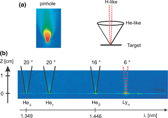

  

  Space-resolved plasma jets consisting of highly charged radiating aluminum ions. a X-ray pinhole image (left) and schematic geometry of the jet emission (right), b two-dimensional X-ray imaging realized with a spherically curved Bragg crystal

The two-dimensional X-ray imaging realizes a two-dimensional spatial resolution with one axis in the Z-direction of the laser propagation while the other direction is along the wavelengths scale. Therefore, the spectral resolution is limited. The key point in the experimental realization is to slightly defocus the spectrometer so that spatial resolution along the wavelengths axis is obtained but to tune the defocusing in a manner to maintain still a spectral resolution that allows identifying the line transitions of interest.

Figure 10.41 shows the spatial variation of the plasma jet emission in colliding plasmas when a highly ionized plasma jet interacts with the residual gas in the target chamber (Rosmej et al. 2006c). The upper part of Fig. 10.41 shows the geometry and the X-ray pinhole emission of the rear-side and front-side emissions. The lower part of Fig. 10.41 shows the two-dimensional X-ray imaging that allows resolving particular line emission (spectral resolution) along with spatial resolution. The spatial variation of the resonance and intercombination lines is drastically different. Moreover, usually very weak intercombination satellite transitions originating from the 1s[2p^{2 3}P] ⁴P-states show very large intensities. These changes are induced by charge transfer process from the low-charged residual gas to the highly ionized plasma jets (Rosmej et al. 2006c). Therefore, space-resolved X-ray spectroscopy has identified charge exchange coupling between the colliding plasmas (jet and residual gas).

Fig. 10.41

X-ray pinhole emission and two-dimensional X-ray imaging of highly charged aluminum plasma jet interaction with the residual gas. Rear-side and front-side emission show characteristic differences that depend on the particular X-ray transition

The detailed spatial information of the radiating plasma jets provides a unique characterization of (a) the interaction between the jet and the residual gas, and (b) their mutual coupling via charge transfer. Therefore, charge exchange is also of considerable interest in high-density plasmas to shed more light into the complex theory of colliding plasmas.

10.5.2 Energy Distribution of Fast Ions

A further important application of space-resolved spectroscopy is the experimental determination of the energy distribution function of fast ions in dense laser-produced plasmas measured via line shifts of spectrally highly resolved resonance lines. These shifts are induced by the directionally Doppler shift. Figure 10.42a shows schematically the principal geometrical arrangement of the measurement. The measurements request two identical spectrometers positioned at very small and at large angles. The comparison of these two spectra then allows attributing the observed relative shift to the fast ion velocity. Figure 10.42b shows the line profile of the H-like fluorine Ly_α and the strongly pronounced “blue” line wing. The Doppler shifted position which corresponds to an ion energy of E = 3.6 MeV is indicated.

Fig. 10.42

a Schematic geometrical arrangement of fast ion Doppler shift measurements of X-ray spectral lines. The first spectrometer is positioned at very low angle $\alpha \approx 0$ while the second spectrometer is located typically at angles $\alpha > 30^\circ$. b The comparison of these two spectra allows deducing shifts originating from the fast ion velocities

Fast ion velocity distribution functions can then be deduced from the optically thin part of the Doppler shifted emission. Figure 10.43 shows that the ion velocity distribution function is reasonably approximated by a unidirectional Maxwellian function with a temperature parameter of kT_ion = 1.35 MeV (Rosmej et al. 1999c, 2002b). These types of measurements provide critical information to test kinetic plasma simulations.

Fig. 10.43

Experimental determination of the fast ion distribution function from the optically thin part of the Doppler shifted emission. The distribution function is reasonably well approximated with a Maxwellian function with a temperature parameter kT_ion = 1.35 MeV

Figure 10.44 shows the space-resolved Doppler line shift measurements for different laser irradiation conditions employing a laser pulse with duration 15 ns, laser wavelength 1.06 μm, and laser energy of 10–60 J. The different focus conditions are realized via different positions of the focusing lens. Also seen from Fig. 10.44 is a correlation of the spatial extension of the spectrally resolved plasma jets (Z-axis, direction of the expanding plasma) and the X-ray pinhole measurements (Fig. 10.44).

Fig. 10.44

Space-resolved X-ray emission (left) and X-ray pinhole emission (right) of highly charged fluorine plasma jet in dependence of different focal lens positions. At highest intensities, the Doppler shift of the He-like resonance line W is very pronounced

Fast ion velocities in dense plasmas lead to differential shifts of emission and absorption coefficients which may lead to considerable modification of optically thick lines shapes as discussed in Sect. 1.1.4 (Fig. 1.4). For this reason, the analysis of the energy distribution function as discussed in Fig. 10.43 has been limited to the line wings, which are optically thin.

Fast ion velocities may also contribute directly to excitation and ionization processes via the W-matrix in the atomic population kinetics. Important examples are the redistribution of population in the fine structure of H-like ions (2s ²S_1/2, 2p ²P_1/2, 2p ²P_3/2) due to a collisional coupling of the 2s ²S_1/2 and 2p ²P_1/2 levels. Their energy difference is very small (Lamb shift), and heavy particle collisions are therefore effective. Other examples are the collisional proton ionization of hydrogen levels with large principal quantum numbers, which turned out to be an important effect in magnetic fusion research (Rosmej and Lisitsa 1998) to analyze charge exchange processes (see Sects. 10.3.1 and 10.3.2).

A very rough estimate of the importance of collisional cross sections induced by fast ions can be made (in some cases) via the classical approach: If the ion velocity V_ion is much smaller than the effective Bohr velocity V_n for an electron with principal quantum number n, the ion-induced cross section might be negligible:

$$\sigma \approx 0: V_{\text{ion}} \ll V_{\text{n}} = V_{0} \displaystyle\frac{{Z_{\text{eff}} }}{n}.$$

(10.157)

V₀ is the Bohr velocity (2.19 × 10⁸ cm/s) and Z_eff is the effective charge of the target ion where the atomic transitions are induced. More detailed calculations of heavy particle collisional cross sections are proposed (Sobelman and Vainshtein 2006; Gryzinsky 1965).

10.6 Atomic Physics in Dense Plasmas with X-ray Free Electron Lasers

XUV and X-ray Free Electron Lasers (XFELs) have provided the high-energy-density physics community with outstanding tools to investigate and to create matter under extreme conditions never achieved in laboratories so far. The key parameters of existing XFEL installations (LCLS in USA, EU-XFEL in Germany, SACLA in Japan) are micro- and even sub-microfocusing to achieve intensities in access to 10¹⁶ W/cm², short pulse lengths (10–100 fs), tunable photon energy (1–30 keV), small bandwidth (some 10 eV at about 10 keV in SASE mode and about 1 eV in self-seeded mode), and high repetition frequency (some 10 Hz up to 100 Hz), allowing to accumulate thousands of shots to improve signal-to-noise ratios.

This makes XFEL installations distinct different from well-known synchrotron radiation facilities. The brilliance of XFEL’s is more than ten orders of magnitude higher than modern synchrotrons, and this allows to photoionize inner-shells of almost every atom in a solid crystal in a single pulse. As the pulse duration is of the order of the Auger time scale an exotic state of matter, a “Hollow Crystal” can be created. The decay of crystalline order can be initiated by a burst of Auger electrons with energies in the X-ray range that heat up the hollow crystal as identified with high-resolution spectroscopy (Galtier et al. 2011) in the first high-energy-density experiment at the XUV–FEL FLASH (Riley et al. 2009). This is distinct different to synchrotrons: Auger electron production is rare compared to the total number of atoms, and Auger electrons do not allow changing the physical properties of the crystal.

Next, the tunable photon energy combined with the small bandwidth permits to pump selected atomic transitions in the X-ray range. Compared to the well-known pumping of low energy transitions by optical lasers, X-ray pumping will allow outstanding steps forward. The first experiment of X-ray pumping of dense plasmas that have been produced by a powerful auxiliary optical laser has been performed at LCLS at SXR (Seely et al. 2011). In this experiment, it has successfully been demonstrated that efficient changes in the atomic populations of highly charged ions induced by XFEL can be achieved (Moinard et al. 2013; Rosmej et al. 2016). As it has been the case for laser-induced fluorescence (LIF) with standard optical lasers, a revolutionary impact is expected via the photopumping of X-ray transitions. In addition to standard LIF, X-LIF will allow to study isoelectronic sequences due to the large range of tunability of the XFEL photons. As synchrotrons might not allow selective efficient X-ray pumping (drastic change of atomic populations), XFEL facilities have opened a new world for scientific activity.

An important further technical process has been made at XFEL’s by reducing the width of the energy distribution function: In the so-called seeded-mode, a bandwidth down to some eV is reached at some keV photon energies. This has led to the first experiment to scan X-ray line shapes in dense plasmas (created with a powerful auxiliary optical laser) at LCLS at MEC (Rosmej et al. 2018).

10.6.1 Scaling Laws to Move Atomic Populations with XFEL

10.6.1.1 Description of Time- and Energy-Dependent XFEL Radiation

Let us assume that time and energy dependence of the XFEL radiation are independent from each other and can therefore be described by the functions $f_{\text{FEL}} \left( t \right)$ and $\tilde{N}_{\text{FEL}} \left( E \right)$. The number of photons per volume/time/energy is then given by:

$$\tilde{N}_{\text{FEL}} \left( {E,t} \right) = \tilde{N}_{\text{FEL}} \left( E \right)f_{\text{FEL}} \left( t \right),$$

(10.158)

$$\int\limits_{ - \infty }^{ + \infty } {f_{\text{FEL}} \left( t \right){\text{d}}t = 1}.$$

(10.159)

We assume a Gaussian energy dependence to simulate the narrow bandwidth of the XFEL:

$$\tilde{N}_{\text{FEL}} \left( E \right) = \tilde{N}_{0} \displaystyle\frac{1}{{\sqrt \pi\Gamma _{\text{FEL}} }}\exp \left( { - \displaystyle\frac{{\left( {E - E_{\text{FEL}} } \right)^{2} }}{{\Gamma _{\text{FEL}}^{2} }}} \right),$$

(10.160)

$$\Gamma _{\text{FEL}} = \delta E/2\sqrt {\ln 2}.$$

(10.161)

$E_{\text{FEL}}$ is the central energy of the radiation field, $\tilde{N}_{\text{FEL}} \left( E \right)$ is the number of photons/volume/energy, $\tilde{N}_{0}$ is the peak number of photons/volume, δE is the bandwidth. Assuming a Gaussian time dependence, the number of photons $N_{{\text{tot},\tau }}$ per pulse length $\tau$ is given by

$$N_{{\text{tot},\tau }} = \int\limits_{0}^{\infty } {{\text{d}}E\int\limits_{\text{volume}}^{{}} {{\text{d}}V} \int\limits_{ - \tau /2}^{ + \tau /2} {{\text{d}}t \,\tilde{N}_{\text{FEL}} \left( {E,t} \right)} }\, \ \approx 2A c \tau \tilde{N}_{0} \,{erf}\left( {\sqrt {\ln 2} } \right) \approx 0.761 \cdot A c \tau \tilde{N}_{0}.$$

(10.162)

$A$ is the focal spot area, $\tau$ is the XFEL pulse width (FWHM). For estimations, the error function can be approximated by

$$\begin{aligned} {erf}(x) & = \displaystyle\frac{1}{\sqrt \pi }\int\limits_{0}^{x} {{e}^{{ - t^{2} }} \cdot {\text{d}}t} \\ & \approx \displaystyle\frac{1}{2} - \displaystyle\frac{{{e}^{{ - x^{2} }} }}{2} \cdot \left[ {\displaystyle\frac{0.3480242}{1 + 0.47047 \cdot x} - \displaystyle\frac{0.0958798}{{\left( {1 + 0.47047 \cdot x} \right)^{2} }} + \displaystyle\frac{0.7478556}{{\left( {1 + 0.47047 \cdot x} \right)^{3} }}} \right]. \\ \end{aligned}$$

(10.163)

The laser intensity $\tilde{I}_{\text{FEL}} \left( {E,t} \right)$ per bandwidth energy and time interval is related to the photon density $\tilde{N}_{\text{FEL}} \left( {E,t} \right)$ via

$$\tilde{I}_{\text{FEL}} \left( {E,t} \right){\text{d}}E{\text{d}}A{\text{d}}t = \tilde{N}_{\text{FEL}} \left( {E,t} \right)E \cdot {\text{d}}E{\text{d}}V{\text{d}}t.$$

(10.164)

Integrating the XFEL beam over a full width at half maximum with respect to energy and time, $\bar{I}_{{\text{FEL},\delta E,\tau }}$ (energy/time/surface) is given by (assuming a Gaussian time dependence):

$$\bar{I}_{{\text{FEL},\delta E,\tau }} = \int\limits_{ - \delta E/2}^{\delta E/2} {{\text{d}}E\int\limits_{ - \tau /2}^{\tau /2} {c\cdot{\text{d}}t} }\,\, E \cdot \tilde{N}\left( {E,t} \right) \approx 4E_{\text{FEL}} c\tilde{N}_{0} {erf}^{2} \left( {\sqrt {\ln 2} } \right) \approx 0.579 \cdot c \cdot E_{\text{FEL}} \cdot \tilde{N}_{0}$$

(10.165)

or, in convenient units

$$\bar{I}_{{\text{FEL},\delta E,\tau }} \approx 2.8\times 10^{ - 9} \left( {\displaystyle\frac{{\tilde{N}_{0} }}{{{cm}^{3} }}} \right)\left( {\displaystyle\frac{{E_{\text{FEL}} }}{{eV}}} \right)\left[ {\displaystyle\frac{\text{W}}{{\text{cm}^{2} }}} \right].$$

(10.166)

The number of photons $N_{{\text{tot},\tau }}$ is related to the intensity $\bar{I}_{{\text{FEL},\tau }}$ via (d is the focal spot diameter)

$$\bar{I}_{{\text{FEL},\tau }} = 2 \cdot {erf}\left( {\sqrt {\ln 2} } \right) \cdot \displaystyle\frac{{N_{{\text{tot},\tau }} \cdot E_{\text{FEL}} }}{{\pi \tau \cdot d^{2} /4}} \approx \displaystyle\frac{{N_{{\text{tot},\tau }} \cdot E_{\text{FEL}} }}{{\tau \cdot d^{2} }}.$$

(10.167)

10.6.1.2 Photoionization

In order to change atomic populations by irradiation of matter with XFEL, photoionization rates need to be larger than corresponding electron ionization rates and, in case of photopumping, photoexcitation rates need to be larger than corresponding spontaneous radiative decay rates. In order to obtain analytical formulas, we consider the hydrogen-like approximation for an arbitrary atom with effective charge $Z_{\text{eff}}$ and an atomic level with principal quantum number $n$ and energy

$$E_{\text{n}} = \displaystyle\frac{{Z_{\text{eff}}^{2} \cdot {Ry}}}{{n^{2} }},$$

(10.168)

where ${Ry} = 13.6057\,{\rm eV}.$ For the case of photoionization this leads to the following relation:

$$\int\limits_{ - \tau /2}^{ + \tau /2} {{\text{d}}t} \int\limits_{{E_{\text{n}} }}^{\infty } {{\text{d}}E \sigma_{\text{n}}^{iz} \left( E \right) c \tilde{N}_{\text{FEL}} \left( {E,t} \right)} > n_{\text{e}} I_{\text{n}}.$$

(10.169)

$\sigma_{\text{n}}^{iz} \left( {E_{\text{FEL}} } \right)$ is the photoionization cross section from level $n,n_{\text{e}}$ is the electron density, $I_{\text{n}}$ is the electron collisional ionization rate, $c$ the speed of light. Employing the Kramers classical cross section for the photoionization (see also Sects. 3.3 and 3.7 and review [Rosmej et al. 2020b]),

$$E > E_{\text{n}} : \sigma_{\text{n}}^{\text{iz}} \left( E \right) = 2.9 \times 10^{ - 17} \displaystyle\frac{{E_{\text{n}}^{5/2} }}{{Z \cdot E^{3} }} \,\left[ {\text{cm}^{2} } \right]$$

(10.170)

and the Lotz-formula for the electron collisional ionization (see Sect. 5.3.1), i.e.,

$$I_{\text{n}} = 6 \times 10^{ - 8} \cdot \left( {\displaystyle\frac{{Ry}}{{E_{\text{n}} }}} \right)^{3/2} \cdot \sqrt {\beta_{\text{n}} } \cdot {e}^{{ - \beta_{\text{n}} }} \cdot \ln \left[ {1 + \displaystyle\frac{{0.562 + 1.4\beta_{\text{n}} }}{{\beta_{\text{n}} \left( {1 + 1.4\beta_{\text{n}} } \right)}}} \right] \left[ {\text{cm}^{3} \text{s}^{ - 1} } \right],$$

(10.171)

$$\beta_{\text{n}} = \displaystyle\frac{{E_{\text{n}} }}{{kT_{\text{e}} }}.$$

(10.172)

Equations (10.168)–(10.172) provide the following estimate (peak intensity $I_{\text{FEL}} = cE_{\text{FEL}} \tilde{N}_{0}$):

$$I_{\text{FEL}} > 3 \times 10^{ - 8} \cdot n_{\text{e}} \left( {\text{cm}^{ - 3} } \right) \cdot Z \cdot \sqrt {\beta_{\text{n}} } \cdot {e}^{{ - \beta_{\text{n}} }} \cdot \ln \left[ {1 + \displaystyle\frac{{0.562 + 1.4\beta_{\text{n}} }}{{\beta_{\text{n}} \left( {1 + 1.4\beta_{\text{n}} } \right)}}} \right] \, \left[ {\displaystyle\frac{\text{W}}{{\text{cm}^{2} }}} \right]$$

(10.173)

assuming $E_{\text{FEL}} = E_{\text{n}} + 3\delta E(\delta E \ll E_{\text{FEL}} )$ for effective photoionization. For $n_{\text{e}} = 10^{21} \,\text{cm}^{ - 3}$, $Z_{\text{eff}} = 13$, $\beta_{\text{n}} = 2$ (10.173) delivers $I_{\text{FEL}} > 3 \times 10^{13}\, \text{W/cm}^{2}$.

10.6.1.3 Photoexcitation

Let us now consider the relations for the X-ray photopumping of line transitions (i.e., resonant photopumping). In order to influence strongly via photoexcitation on the atomic populations, photoexcitation rates need to be larger than corresponding spontaneous radiative decay rates:

$$\int\limits_{ - \tau /2}^{ + \tau /2} {{\text{d}}t} \int\limits_{{\Delta E_{\text{nm}} - \delta \tilde{E}/2}}^{{\Delta E_{\text{nm}} + \delta \tilde{E}/2}} {{\text{d}}E \, \sigma_{\text{nm}}^{\text{abs}} \left( E \right) c \tilde{N}_{\text{FEL}} \left( {E,t} \right)} \ge A_{\text{mn}}.$$

(10.174)

$\sigma_{\text{nm}}^{\text{abs}} \left( E \right)$ is the photoabsorption cross section for the transition from level $n$ to level $m$ and $A_{\text{mn}}$ is the spontaneous radiative decay rate from level $m$ to level $n,\delta \tilde{E}$ is an effective width for the XFEL interaction with the atomic transition. The photoabsorption cross section is given by

$$\sigma_{\text{nm}}^{\text{abs}} \left( E \right) = \displaystyle\frac{E}{4\pi }B_{\text{nm}} \varphi_{\text{nm}} \left( E \right).$$

(10.175)

$B_{\text{nm}}$ is the Einstein coefficient of stimulated absorption that is related to the Einstein coefficient of spontaneous radiative decay according to

$$B_{\text{nm}} = \displaystyle\frac{{4\pi^{3} \hbar^{3} c^{2} }}{{E^{3} }}\displaystyle\frac{{g_{\text{m}} }}{{g_{\text{n}} }}A_{\text{mn}},$$

(10.176)

$\varphi_{\text{nm}} \left( E \right)$ is the normalized local absorption line profile:

$$\int\limits_{ - \infty }^{ + \infty } {\varphi_{\text{nm}} \left( E \right){\text{d}}E} = 1.$$

(10.177)

We assume a Gaussian line profile with full width at half maximum, i.e.,

$${FWHM} = 2\sqrt {\ln 2 }\,\Gamma _{\text{G}}$$

(10.178)

and a width parameter

$$\Gamma _{\text{G}} = \Delta E_{\text{nm}} \sqrt {2kT_{\text{i}} /Mc^{2} }$$

(10.179)

corresponding to a Doppler profile to obtain analytical estimates:

$$\varphi_{\text{nm}} \left( E \right) = \displaystyle\frac{1}{{\sqrt\pi \,\Gamma _{\text{G}} }}\exp \left[ { - \left( {\displaystyle\frac{{E - \Delta E_{\text{nm}} }}{{\Gamma _{\text{G}} }}} \right)^{2} } \right]$$

(10.180)

and ($\delta {\tilde E}$ is the bandwidth)

$$\displaystyle\frac{4\ln 2}{{\delta \tilde{E}^{2} }} = \displaystyle\frac{1}{{\Gamma _{\text{G}}^{2} }} + \displaystyle\frac{1}{{\Gamma _{\text{FEL}}^{2} }}.$$

(10.181)

If the XFEL photon energy is exactly tuned to the transition energy, e.g., $E_{\text{XFEL}} = \Delta E_{\text{nm}}$ $E_{\text{XFEL}} = \Delta E_{\text{nm}}$, (10.160), (10.161), (10.174)–(10.181) provide the following estimate:

$$I_{\text{FEL}} > 2 \times 10^{5} \Delta E_{\text{nm}}^{3} \displaystyle\frac{{g_{\text{n}} }}{{g_{\text{m}} }}\sqrt {{FWHM}_{\text{FEL}}^{2} + {FWHM}_{\text{G}}^{2} } \,\left[ {\displaystyle\frac{\text{W}}{{\text{cm}^{2} }}} \right]$$

(10.182)

with $\Delta E_{\text{nm}}$ and FWHM in [eV]. For H-like Al Ly_α, $\Delta E_{\text{nm}} = 1728\,\text{eV}$, $g_{\text{n}} = 2$, $g_{\text{m}} = 6$, we obtain $I_{\text{XFEL}} = 4 \times 10^{15} \,\text{W/cm}^{2}$ (assuming $\sqrt {{FWHM}_{\text{FEL}}^{2} + {FWHM}_{G}^{2} } = 10\,\text{eV}$). The relation (10.182) indicates an important scaling law:

$$I_{\text{FEL}} \propto Z^{6}.$$

(10.183)

Therefore, extremely high brilliance of XFEL’s is needed to pump X-ray transitions. Assuming a spot diameter of $d = 2\,\upmu \text{m}$, pulse length $\tau = 100\,\text{fs}$, photon energy $E_{\text{XFEL}} = 1.7\,\text{keV}$ and a laser intensity of $\bar{I}_{{\text{FEL},\tau }} = 10^{16} \,\text{W/cm}^{2}$, a minimum of about $N_{{\text{tot},\tau }} = 2 \times 10^{11} \,\text{photons}$ in the XFEL pulse is requested according (10.167) to effectively move atomic populations in the X-ray energy range. Currently operating/planed Free Electron Laser facilities fulfill these requirements. We note that relation (10.183) does not depend on the electron density and the intensity estimate holds therefore true for low- and high-density plasmas.

10.6.2 Atomic Kinetics Driven by Intense Short Pulse Radiation

Radiation field quantum mechanics in second quantization (Heitler 1954; Pike and Sarkar 1995) and quantum kinetics (Rautian and Shalagin 1991) is the most general approach to study the interaction of radiation fields with atoms while the quantum kinetic approach via the density matrix theory (see Chap. 7) is the most general approach to determine atomic populations (that are at the heart of almost all properties of matter). On a unique footing, these approaches allow describing atomic population and coherences and provide all necessary quantum matrix elements to take into account the relevant elementary atomic processes (cross sections) and field-atom interactions.

Under the assumption of broadband illumination and/or large collisional broadening, the non-diagonal density matrix elements are negligible compared to the diagonal ones (atomic populations) and the so-called rate equation atomic population kinetic approach becomes valid (Loudon 2000). In order to keep the presentation transparent, we employ for the below presentation the rate equation kinetics in its most general form as outlined in Chap. 6. This approach will be supplemented below to take into account an external intense short pulse radiation field to describe the XFEL interaction with matter. We therefore start from (6.22)–(6.28); however, the transition matrix elements have to be supplemented with a radiation field term driven by the XFEL, i.e.,

$$W_{\text{ji}} = W_{\text{ji}}^{\text{col}} + W_{\text{ji}}^{\text{rad}} + W_{\text{ji}}^{\text{FEL}}.$$

(10.184)

The radiation field matrix elements $W_{\text{ji}}^{\text{FEL}}$ for the external XFEL radiation are given by

$$W_{\text{ji}}^{\text{FEL}} = W_{\text{ji}}^{\text{FEL,PI}} + W_{\text{ji}}^{\text{FEL,SR}} + W_{\text{ji}}^{\text{FEL,SA}} + W_{\text{ji}}^{\text{FEL,SE}},$$

(10.185)

$$W_{\text{ji}}^{\text{FEL,PI}} = \int\limits_{{\hbar \omega_{\text{ji}} }}^{\infty } {{\rm{d}}\left( {\hbar \omega } \right)\sigma_{\text{ji}}^{\text{PI}} \left( {\hbar \omega } \right)c\tilde{N}\left( {\hbar \omega } \right)},$$

(10.186)

$$W_{\text{ji}}^{\text{FEL,SR}} = n_{\text{e}} \displaystyle\frac{{\pi^{2} c\hbar^{3} }}{{\sqrt 2 m_{\text{e}}^{3/2} }}\displaystyle\frac{{g_{\text{i}} }}{{g_{\text{j}} }}\int\limits_{0}^{\infty } {{\text{d}}E \,\displaystyle\frac{F\left( E \right)}{\sqrt E }\,\sigma_{\text{ji}}^{\text{PI}} \left( {\hbar \omega_{\text{ji}} + E} \right)\tilde{N}\left( {\hbar \omega_{\text{ji}} + E} \right)},$$

(10.187)

$$W_{\text{ji}}^{\text{FEL,SA}} = \pi^{2} c^{3} \hbar^{3} A_{\text{ji}} \displaystyle\frac{{g_{\text{j}} }}{{g_{\text{i}} }}\int\limits_{0}^{\infty } {\text{d}\left( {\hbar \omega } \right)\displaystyle\frac{{\varphi_{\text{ji}} \left( \omega \right)}}{\hbar }\displaystyle\frac{{\tilde{N}\left( {\hbar \omega } \right)}}{{\left( {\hbar \omega } \right)^{2} }}},$$

(10.188)

$$W_{\text{ji}}^{\text{FEL,SE}} = \pi^{2} c^{3} \hbar^{3} A_{\text{ji}} \int\limits_{0}^{\infty } {\text{d}\left( {\hbar \omega } \right)\displaystyle\frac{{\varphi_{\text{ji}} \left( \omega \right)}}{\hbar }\displaystyle\frac{{\tilde{N}\left( {\hbar \omega } \right)}}{{\left( {\hbar \omega } \right)^{2} }}}.$$

(10.189)

$W_{\text{ji}}^{\text{FEL,PI}}$ describes photoionization, W^FEL,SR stimulated radiative recombination, $W_{\text{ji}}^{\text{FEL,SA}}$ stimulated photoabsorption, $W_{\text{ji}}^{\text{FEL,SE}}$ stimulated photoemission. $\sigma_{\text{ji}}^{\text{PI}}$ is the photoionization cross section, $F\left( E \right)$ the energy distribution function of the continuum electrons, $A_{\text{ji}}$ the Einstein coefficient of spontaneous emission, $\varphi_{\text{ji}}$ the line profile, $c$ the speed of light, $\hbar$ is the Planck constant, $g_{\text{i}}$ the statistical weight of a bound state, $\omega$ the angular frequency of the external radiation field, $\omega_{\text{ji}}$ the atomic transition frequency, and $\tilde{N}$ is the number of external photons (those of the Free Electron Laser) per unit volume and energy. We note, that (10.186–10.189) assume that the concept of standard ionization and excitation probability per unit time in Fermi’s golden rule and in Einstein’s theory of stimulated emission and absorption is still valid. This assumption breaks down for ultra-short pulses [Rosmej et al. 2021]: numerical calculations carried out in terms of a generalized probability for the total duration of pulses in the near-threshold regime demonstrate essentially non-linear behavior, while absolute values may change by orders of magnitude for typical ultra-short XFEL and High-Harmonic Generated HHG pulses [Rosmej et al. 2021].

In optically thick plasmas, the spectral intensity distribution of an atomic transition $i \to j$ with frequency $\omega_{\text{ji}}$ is given by (see also Sect. 1.1.4):

$$I_{{j_{\text{Z}} i_{\text{Z}} }} \left( \omega \right) = \displaystyle\frac{{\hbar \omega_{{j_{\text{Z}} i_{\text{Z}} }} }}{4\pi } \cdot n_{{j_{\text{Z}} }} \cdot A_{{j_{\text{Z}} i_{\text{Z}} }} \cdot\Lambda _{{j_{\text{Z}} i_{\text{Z}} }} \cdot \Phi_{{j_{\text{Z}} i_{\text{Z}} }} \left( {\omega ,\omega_{{j_{\text{Z}} i_{\text{Z}} }} } \right).$$

(10.190)

$n_{{j_{\text{Z}} }}$ is the population of the upper-level j, $A_{{j_{\text{Z}} i_{\text{Z}} }}$ is the spontaneous transition probability for the transition $j \to i$, $\Lambda _{{j_{\text{Z}} i_{\text{Z}} }}$ is the lambda-operator to describe radiation transport effects [Sect. 1.1.4, e.g., (1.33)] and $\Phi_{{j_{\text{Z}} i_{\text{Z}} }} \left( {\omega ,\omega_{{j_{\text{Z}} i_{\text{Z}} }} } \right)$ is the associated optically thick emission line profile (see Sect. 1.1.4, (1.34)). Equation (10.190) indicates a strong interplay between the atomic structure (means transition probabilities $A_{{j_{\text{Z}} i_{\text{Z}} }}$) and atomic populations kinetics (population densities $n_{{j_{\text{Z}} }}$). The total spectral local distribution is then given by

$$I\left( \omega \right) = \sum\limits_{Z = 0}^{{Z_{\text{n}} }} {\sum\limits_{{j_{\text{Z}} = 1}}^{{N_{\text{Z}} }} {\sum\limits_{{i_{\text{Z}} = 1}}^{{N_{\text{Z}} }} {I_{{j_{\text{Z}} i_{\text{Z}} }} \left( \omega \right)} } }.$$

(10.191)

Equation (10.191) is of great practical interest: It is the spectral distribution that is accessible via X-ray spectroscopic measurements. In plasmas where opacity in line transitions is important $\Lambda _{{j_{\text{Z}} i_{\text{Z}} }} < 1$ and a generalized optically thick line profile has to be invoked (see (1.34) of Sect. 1.1.4). If also radiation transport in the continuum is important, the generalized radiation transport equation has to be solved (Mihalas 1978). Such experimental situations, however, should be avoided: The photon absorption in the continuum of a line transition is not at all redistributed in the line itself, but redistributed in a large spectral interval due to the large “width” of the continuum (in other words the “line photon” is lost). Therefore, under such circumstances diagnostic ratios would rather be meaningless than useful. In order to properly design experiments that avoid radiation transport in the continuum, the continuum opacities $\tau_{\text{ff}}$ (free–free opacity) and $\tau_{\text{fb}}$ (free–bound opacity) should be $\tau_{\text{ff}} < 0.01$ and $\tau_{\text{fb}} < 0.01$ (the opacities can be estimated from (1.54) and (1.55). It is also desirable to avoid as much as possible the bound–bound opacity and ensure $\tau_{\text{ji}} \, <\, 0.1$ (see, e.g., (1.56), (1.57)). This strong estimate is related to the fact that in most cases of XFEL research, X-ray transitions from autoionizing states are recorded: Radiation transport related to autoionizing levels is very harmful for spectroscopic diagnostic studies, as the reemission after absorption is almost suppressed due to the large autoionizing rates (Kienle et al. 1995), i.e., a small branching factor

$$p_{\text{ji}} = \left( {\displaystyle\frac{{A_{\text{ji}} }}{{\sum\nolimits_{l} {A_{\text{jl}} } + \sum\nolimits_{k} {\Gamma _{\text{jk}} } + \sum\nolimits_{m} {C_{\text{jm}} } }}} \right)^{{N_{\text{ji}} }}.$$

(10.192)

$p_{\text{ji}}$ is the probability that a photon from a line transition $j \to i$ is reemitted, $A_{\text{ji}}$ is the radiative decay, $\sum\nolimits_{l} {A_{\text{jl}} } ,\sum\nolimits_{k} {\Gamma _{\text{jk}} }$ and $\sum\nolimits_{m} {C_{\text{jm}} }$ are the total radiative decay rates, autoionizing rates and collisional rates leading to a depopulation of the upper-level $j ,$ and $N_{\text{ji}}$ is the number of photon scatterings. As an example let us consider aluminum and the j-dielectronic satellite (discussed in Table 10.1): $A_{\text{ji}} = 1.31 \times 10^{13}\, \text{s}^{ - 1} ,\Gamma _{\text{jk}} = 1.29 \times 10^{14}\, \text{s}^{ - 1}$. Even if we set $\sum\nolimits_{m} {C_{\text{jm}} } = 0$ the remission probability is very low, $p_{\text{ji}} = 9.18 \times 10^{ - 2}$.

Finally we note that bound–bound opacity of a transition that is emitted, absorbed, and reemitted in a dense plasma should not be confused with the opacity of XFEL-induced resonant pumping.

10.6.3 Interaction of XFEL with Dense Plasmas

10.6.3.1 General Features of XFEL Interaction with Dense Plasmas: Simulations

Figure 10.45 shows an experimental scheme for a typical pump probe experiment. A powerful optical laser is irradiating a solid target to create a dense plasma plume. The target is mounted on a rotating cylinder in order to accumulate spectra to improve the signal-to-noise ratio. The XFEL is then triggered with respect to the optical laser and focused into the dense plasma plume to pump X-ray transitions. A high-resolution (high spectral and spatial) X-ray spectrometer is employed to record the spectral distribution of the pumped X-ray transitions in dependence of the target distance (along Y-axis in Fig. 10.45).

Fig. 10.45

Principle scheme of a pump probe experiment when intense XFEL radiation interacts with dense plasma produced by a powerful auxiliary optical laser

Let us follow the principle steps of XFEL interaction with a dense plasma with the MARIA simulations described above taking also into account all radiation field terms of (10.184)–(10.189) and a detailed LSJ-split atomic atomic/ionic level system including ground, single, and multiple excited and hollow ion states from various charge states (Rosmej and Lee 2007).

Figure 10.46 shows the evolution of the average charge (solid curve) when an intense pulsed radiation field (dashed curve) is interacting with dense magnesium plasma:

Fig. 10.46

MARIA simulations of the temporal evolution of the XFEL pulse and the average charge state of a dense Mg plasma, E_FEL = 1850 eV, τ = 100 fs, I_max = 2.2 × 10¹⁷ W/cm², n_e = 10²¹ cm⁻³, kT_e = 40 eV, L_eff = 10 μm

$$\left\langle Z \right\rangle = \sum\limits_{Z = 0}^{{Z_{\text{n}} }} {n_{\text{Z}} Z},$$

(10.193)

where $n_{\text{Z}}$ is the ionic population of charge Z (see (6.29)). The plasma density is $n_{\text{e}} = 10^{21}\, \text{cm}^{ - 3}$, the temperature $kT_{\text{e}} = 40\,\text{eV}$. Opacity effects of the internal atomic/ionic radiation are included via an effective photon path length of L_eff = 10 µm (see Sect. 1.1.4). The XFEL pulse duration is $\tau = 100\,\text{fs}$, photon energy $E_{\text{XFEL}} = 1850\,\text{eV}$ and the photon density is $\tilde{N}_{0} = 10^{23} \,\text{cm}^{ - 3}$. The maximum laser intensity is then

$$I_{{\max} } = cEf_{{\text{FEL},{\max} }} \cdot \tilde{N}_{0} = 4.8\,\times\,10^{ - 9} f_{{\text{FEL},{\max} }} \left( {\displaystyle\frac{{\tilde{N}_{0} }}{{\text{cm}^{3} }}} \right)\left( {\displaystyle\frac{E}{\text{eV}}} \right)\left[ {\displaystyle\frac{\text{W}}{{\text{cm}^{2} }}} \right],$$

(10.194)

where $f_{{\text{XFEL},\,{\max} }}$ is the maximum value ($f_{{\text{XFEL},\,{\max} }} = 0.246$ in Fig. 10.46) of the normalized time-dependent function of the laser intensity; see (10.158), (10.159), $I_{{\max} } = 2.2 \times 10^{17} \,\text{W/cm}^{2}$. Before the XFEL pulse interacts with the Mg plasma plume, the average charge state is about $\left\langle Z \right\rangle \approx 7.4$ that rises dramatically during the interaction with the XFEL pulse. The system shows shock characteristics: After laser pulse maximum, the average charge state is still increasing (at about $t = 10^{ - 13} \,\text{s}$), then stays almost constant for a few ps, then decreases on a 100 ps time scale followed by a very slow final equilibration phase (10–100 ns). We note, that general characteristics of shocked atomic systems have been explored in [Deschaud et al. 2020].

Let us follow the shock characteristics in more detail via the ionic populations. Figure 10.47 shows the charge state evolutions of the bare nucleus (nuc), H-like ions (H), He-like ions (He), and Li-like ions (Li). Figure 10.47a shows the case when the photon energy $E_{\text{XFEL}} = 1850\,\text{eV}$ is larger than the ionization potential of the He-like Mg ground state $\left( {E_{\text{i}} \left( {1{s}^{2} \,{}^{1}{S}_{0} } \right) = 1762\,\text{eV}} \right)$. Before the XFEL pulse, the ionic fractions nuc, H, and He are negligibly small due to the low electron temperature of the plasma plume. With the onset of the XFEL pulse, He-like and H-like ionic fractions rise rapidly. The population of the fully stripped Mg (“nuc” in Fig. 10.47a) stays very small, because the XFEL photon energy does not allow direct photoionization of the H-like ground state. The slight rise at the beginning of the XFEL pulse is connected with collisional excitation–ionization processes in the dense plasma.

Fig. 10.47

MARIA simulations of the temporal evolution of the ionic fractions after interaction of the XFEL pulse with a dense Mg plasma plume, a E_FEL = 1850 eV, τ = 100 fs, $\tilde{N}_{0} = 10^{23} \text{cm}^{ - 3}$, I_max = 2.2 × 10¹⁷ W/cm², n_e = 10²¹ cm⁻³, kT_e = 40 eV, L_eff = 30 μm, b E_FEL = 3100 eV, τ = 100 fs, $\tilde{N}_{0} = 10^{23} \text{cm}^{ - 3}$, I_max = 3.7 × 10¹⁷ W/cm², n_e = 10²¹ cm⁻³, kT_e = 30 eV, L_eff = 30 μm

Figure 10.47b shows a simulation when the photon energy is larger than the ionization potential of the H-like ground state. Like in Fig. 10.47a, before the XFEL pulse, the ionic fractions of the bare nucleus, H- and He-like ions are negligibly small due to the low electron temperature of the plasma plume. With the onset of the XFEL pulse, Li-like, He-like, and H-like ionic fractions rise rapidly. At about laser pulse maximum, the fraction of H-, He-, and Li-like ions drop again because the XFEL photons are photoionizing the H-like ground state 1s ²S_1/2 because the photon energy of $E_{\text{XFEL}} = 3100\,\text{eV}$ keV is larger than the ionization potential of H-like Mg ground state $\left ( E_{\text{i}} \left( {1{s}\,{}^{2}{S}_{1/2} } \right) = 1963\,\,\text{eV} \right)$. The depletion of almost all electrons from the atomic system makes the plume transparent to the XFEL radiation as no more absorption is possible: The absorption is saturated. When the pulse is off, H-like, He-like, and Li-like ionic fractions increase as recombination starts from the bare nucleus. At even later times (about t = 10⁻¹⁰ s), all ionic fractions (nuc, H, He, Li) decrease due to the overall cooling of the plume (rise of ionic fractions of low-charged ions not shown in Fig. 10.47b).

Figures 10.47 demonstrate that in the photoionization regime, the tuning of the XFEL beam allows selection of different charge states (i.e., cutoff of charge states that have ground state ionization energies above the photon pumping energy).

10.6.3.2 X-ray Pumping of Dense Plasmas

In the resonant pumping scheme, the tuning of the XFEL energy allows to selectively pump bound–bound transitions and induce corresponding fluorescence, so-called X-ray laser-induced fluorescence, so-called X-LIF (Rosmej et al. 2016, 2022).

Figure 10.48 presents the first X-LIF spectra of dense aluminum plasma observed at LCLS for different X-ray pumping energies and for X-ray pulses delayed by 100 ps (Moinard et al. 2013; Rosmej et al. 2016, 2022). For reference, the upper spectrum (red curve) shows the spectral emission of the Al plasma created by the optical YAG laser only (i.e., X-ray pump was absent). Dominating transitions are the He-like resonance line 1s^{2 1}S₀–1s2p ¹P₁ and the intercombination line 1s^{2 1}S₀–1s2p ³P₁ (W and Y in Fig. 10.48) of 11 times ionized aluminum. XFEL pumping at 1597 eV (curve labeled as “He-like” for pumping of helium-like atomic states) matches the atomic transition W that in turn results in a strong intensity increase (factor 4) of the W-line (note that all spectra have been normalized to the peak intensity).

Fig. 10.48

Experimental spectra of resonant XFEL pumping of dense plasmas produced with an auxiliary optical laser. The upper spectrum (red, linear scale) shows the X-ray emission from the optical laser-produced plasma only that is dominated by the He-like resonance line W and intercombination line Y. The pumping energies (blue numbers, spectral positions indicted with flashes) fall into the spectral window of the X-ray spectral distribution of the K²L^N + E_XFEL → K¹L^N+1 transitions (N = 1–4). The induced emission (solid black curves, linear scale, normalized to peak emission) from the He-like to C-like charge states corresponds to emission from ionic core hole states K¹L^N+1. When the X-ray pump is on, strong intensity rises of X-ray transitions (X-ray laser-induced fluorescence X-LIF) from Li-like until C-like ions are observed. The X-ray pumping moves the intensities by many orders of magnitude

The pumping at lower energies introduces abrupt changes in the spectral distribution. In particular, the pumping at 1587 eV corresponds to the transitions K²L¹ + hν_XFEL → K¹L². The pumped states are therefore the Li-like (10 times ionized aluminum) autoionizing levels 1s2l2l′. Although the transitions that originate from these states are of very low intensity for the upper red curve (no pump), the X-ray pumping results in a strong intensity increase. X-ray pumping at 1570, 1551, and 1531 eV corresponds to X-LIF of the autoionizing Be-like (nine times ionized aluminum) states K¹L³, the B-like (eight times ionized aluminum) states K¹L⁴, and C-like (seven times ionized aluminum) states K¹L⁵. Here, K and L denote the population of the inner atomic shells.

It is important to emphasize that emission lines, being weak or entirely absent in the dense optical laser-produced plasma (e.g., the Be-, B-, and C-like transitions) have been pumped to intensities that exceed even those of the resonance line W (that is not pumped and its occurrence is only due to thermal excitation inside the dense optical laser-produced plasma, upper red curve in Fig. 10.48).

The possibility of strong signal rise in the X-ray range from non-observable intensities to excellent signal-to-noise ratios is further demonstrated in Fig. 10.49. The figure demonstrates a rise in signal levels for the Be-like satellite X-ray transitions by a factor of 300 (the lower red spectrum has been shifted down by a factor of 10 for better comparison) implying that the charge state distribution can be probed in low-temperature dense plasmas (strongly coupled) that would not be observable otherwise.

Fig. 10.49

Experimental spectrum of XFEL pumped dense aluminum plasma at E_XFEL = 1570 eV (indicated with dashed blue line). X-LIF increases the Be-like satellite intensity by about two–three orders of magnitude (compared to the emission from optical laser only, red dotted curve) moving even non-detectable transitions (e.g., the two-electron transitions indicated by blue flash) to excellent signal-to-noise ratios

Figure 10.49 demonstrates likewise that X-LIF can move non-observable bound–bound transitions to excellent signal levels. The two-electron transitions of the Be-like satellites, i.e., 1s2s²2p^{1 1}P₁−1s²2p^{2 1}D₂ are not observable in the spectrum from the dense optical laser-produced plasma (red dotted curve in Fig. 10.49) but moves to a good signal-to-noise ratio due to X-ray pumping.

Figure 10.50 demonstrates transient resonant pumping by setting different delay times between the maximum of the optical laser pulse and the XFEL pulse in the range of Δt = −50 ps to +300 ps. Figure 10.50a shows the spectral distribution in the high-quality X-ray emission spectra of aluminum for Δt = 0 ps. The blue curve shows the best fit from a transient non-LTE simulation carried out with the MARIA collisional–radiative kinetics code described above. The simulations include the exact overlap integrals of line profiles of the atomic transitions and the energy distribution function of the XFEL for resonant and non-resonant pumping. In addition, the XFEL pulse was resolved in time and brought to interaction with the plasma at a given temperature and density. A spectral distribution was then calculated at every time step and then summed up until convergence was reached to compare simulations with data. The simulations presented in Fig. 10.50a (blue curve) are obtained for an electron temperature of 100 eV and electron density of 1 × 10²¹ cm⁻³. Despite a simple zero-dimensional model, the blue curve provides a rather good fit to the measured data. We note that the plasma density is distinctly higher (order of magnitude) than that obtained from the non-LTE fit of the optical laser-produced plasma (upper red curve in Fig. 10.48). This is consistent because XFEL absorption and subsequent X-LIF take place at higher densities for the geometry shown in Fig. 10.45. The spectral distribution is far from LTE, as demonstrated by the comparison of the blue and green curves, cf. Figure 10.50a. Non-LTE effects are therefore important even for high densities because high autoionizing rates and fs time scales do not permit effective collisional redistribution.

Fig. 10.50

Experimental spectra of transient X-ray pumping at different delay times Δt with respect to the optical laser pulse. a Time-dependent non-LTE simulations for Δt = 0 ps carried out with the MARIA code, b experimental X-LIF spectra for Δt = −50 ps and +300 ps

In conclusion, the first transient X-ray pumping of dense optical laser-produced plasmas presented in Figs. 10.48 and 10.49 demonstrates the great potential of X-ray laser-induced fluorescence (X-LIF) in dense plasma atomic physics and high-energy-density physics (Rosmej et al. 2016, 2022).

10.6.4 Beating the Auger Clock

10.6.4.1 Photoionization Versus Autoionization

Photoionization of inner atomic shells creates multiple excited states that can decay via non-radiative transitions. Let us consider the photoionization from the K-shell:

$$K^{2} L^{X} M^{Y} N^{Z} + h\nu_{\text{XFEL}} \to K^{1} L^{X} M^{Y} N^{Z} + e_{\text{photo}}$$

(10.195)

(e.g., iron is described by the configuration K²L⁸M¹⁴N²). The photoionized state is multiple excited and can decay via radiative and non-radiative (autoionization, known as Auger effect in solid-state physics) transitions. Let us consider a simple example (Y = 0, Z = 0):

$$K^{1} L^{X} \to \left\{ {\begin{array}{*{20}l} {{radiative\;decay}:} \hfill & {K^{2} L^{X - 1} + h\nu_{{K_{\alpha } }} } \hfill \\ {{non{-}radiative\;decay}: } \hfill & {K^{2} L^{X - 2} + e_{\text{Auger}} } \hfill \\ \end{array} } \right\}.$$

(10.196)

Radiative and non-radiative decay processes in the X-ray energy range have extensively been studied in the very past (Flügge 1957). Particularly synchrotrons have been employed for advanced studies of X-ray interaction with solid matter. Synchrotron radiation, however, is not very intense, allowing occurrence of photoionization of inner-shells only as a rare process (means a negligible fraction of the atoms in the crystal are photoionized thereby leaving the solid system almost unperturbed). This situation is quite different for XFEL’s outlined above: Their brilliance is more than ten orders of magnitude higher than those of most advanced synchrotrons. Photoionization of inner-shells may therefore concern almost every atom in the crystal structure leading to essential perturbations and corresponding dramatic changes in the physical properties of matter.

In terms of elementary processes, XFEL-driven photoionization rates allow to compete even with the Auger rates (autoionizing rates Γ are very large, order of 10¹²–10¹⁶ s⁻¹). The necessary XFEL intensities to “compete“ with the Auger effect can be estimated according to (see also (10.169)):

$$\int\limits_{ - \tau /2}^{ + \tau /2} {{\text{d}}t} \int\limits_{{E_{\text{n}} }}^{\infty } {{\text{d}}E \sigma_{\text{n}}^{\text{iz}} \left( E \right) c \tilde{N}_{\text{FEL}} \left( {E,t} \right)} >\Gamma.$$

(10.197)

Assuming a photon energy E_FEL of the XFEL which is sufficient to proceed toward effective photoionization, namely E_FEL = E_n + 3δE, (δE ≪ E_n, E_n is the ionization energy of the inner-shell with principal quantum number “n”), we obtain the following estimate:

$$I_{\text{FEL}} > 4 \times 10^{ - 1} \cdot\Gamma \cdot \displaystyle\frac{{Z^{4} }}{{n^{3} }} \left[ {\displaystyle\frac{\text{W}}{{\text{cm}^{2} }}} \right].$$

(10.198)

As autoionizing rates scale approximately like $\Gamma \propto Z^{0}$ (means almost independent of Z in the hydrogenic approximation) the Z-scaling of (10.198) is approximately given by

$$I_{\text{FEL}} \propto Z^{4}.$$

(10.199)

Let us consider the photoionization of the K-shell of Al I as an example: Z ≈ 10.8, n = 1, Γ ≈ 10¹⁴ s⁻¹, I_FEL > 5 × 10¹⁷ W/cm². As microfocusing is a standard setup at the XFEL installations (usually realized with Beryllium lenses), intensities of the order of 10¹⁷ W/cm² can be achieved allowing photoionization of inner-shells to compete with the Auger rate. Also sub-microfocusing was demonstrated employing a four-mirror focusing system in Kirkpatrick–Baez geometry. This allowed to reach focal spot sizes down to 0.05 μm and intensities up to 10²⁰ W/cm² (achieved at the SACLA XFEL (Mimura et al. 2014)). We note that the competition between the photoionization of inner-shells and the autoionization means that the change in atomic populations due to photoionization is essential compared to the Auger rate that destroys the inner-shell excited autoionizing state.

10.6.4.2 Hollow Ion Formation

Apart the threshold intensity of (10.198), the characteristic Auger time scale is another important issue. Before XFEL’s became available for dense plasma physics experiments, it was proposed (Rosmej 2007, Rosmej and Lee 2007) on the basis of simulations carried out with the MARIA code that “beating the Auger clock” will allow massive creation of hollow ions and permit their observation via the characteristic X-ray emission. Let us consider the relevant physics via an example: creation of hollow ion K⁰L^X configurations and corresponding characteristic inner-shell X-ray emission. We start from the K²L^X configurations. Photoionization of the K-shell creates the state

$$K^{2} L^{N} + \hbar \omega_{\text{XFEL}} \to K^{1} L^{N} + e_{{\text{photo},1}}.$$

(10.200)

In order to proceed with interesting processes from the XFEL-produced single hole state K¹L^X, the duration of the XFEL pulse (being responsible for the first photoionization) must be of the order of the characteristic Auger time scale. As the operating VUV/X-ray FEL facilities propose the requested pulse durations (order of 10–100 fs), photoionization may further proceed from the single K-hole state to produce a second K-hole (hollow ion):

$$K^{1} L^{N} + \hbar \omega_{\text{XFEL}} \to K^{0} L^{N} + e_{{\text{photo},2}}.$$

(10.201)

The existence of the double K-hole configuration K⁰L^X can easily be identified via the characteristic hollow ion X-ray transitions that are located approximately between Ly_α and He_α of highly charged ions (Faenov et al. 1999; Rosmej et al. 2015):

$$K^{0} L^{N} \to K^{1} L^{N - 1} + \hbar \omega_{\text{hollow}}.$$

(10.202)

Ab initio calculations with the MARIA code that include radiation field physics (see Sect. 10.6.2) demonstrate that hollow ion production is effective and observable levels of characteristic X-ray emission are achieved. These simulations have lead to a proposal for hollow ion research in dense plasmas at planed XFEL installations (Rosmej 2007, Rosmej and Lee 2007).

The central wavelengths of hollow ion emission groups can be approximated by (Rosmej et al. 2015):

$$\lambda (K^{0} L^{N} \to K^{1} L^{N - 1} ) \approx \displaystyle\frac{{1.215 \times 10^{ - 7}\, {m}}}{{\left( {Z_{\text{n}} - \sigma_{{{Ly}_{\alpha } }} - \sigma_{\text{L}} \times (N - 1)} \right)^{2} }},$$

(10.203)

$$\sigma_{{{Ly}_{\alpha } }} = - a_{1} (Z_{\text{n}} - 3) - a_{3} (Z_{\text{n}} - 3)^{3}$$

(10.204)

with a₁ = 6.17094 × 10⁻⁴ and a₃ = 9.15902 × 10⁻⁶ resulting in an approximation with spectroscopic precision for Z_n = 3–56 (Z_n is the nuclear charge). Equation (10.204) includes the negative screening that is important for higher Z-elements, e.g., for Z_n = 56, σ_Lyα = −1.397. From Hartree–Fock calculations, we obtain a screening constant for the L-shell electrons, σ_L ≈ 0.07 for He-like until O-like ions for each supplementary electron in the L-shell.

In order to estimate which hollow ion transitions are located between the H-like Ly_α and He-like He_α transitions, we can estimate the transition energies in the optical electron model:

$$\Delta E = \displaystyle\frac{3}{4}Z_{\text{eff}}^{2} {Ry},$$

(10.205)

where Ry = 13.6058 eV and the effective charge is given by

$$Z_{\text{eff}} = Z_{\text{n}} - \sigma.$$

(10.206)

Z_n is the nuclear charge and σ is a screening constant. For the He-like resonance line He_α = 1s2p ¹P₁–1s^{2 1}S₀, the screening constant can be approximated by

$$\sigma_{{He_{\alpha } }} = \sigma_{0} - a_{1} (Z_{\text{n}} - 8) - a_{3} (Z_{\text{n}} - 8)^{3},$$

(10.207)

where σ₀ = 0.50417, a₁ = 3.4565 × 10⁻³, a₃ = 1.16632 × 10⁻⁵. The application of this formula results in wavelength calculations with spectroscopic precision for Z_n = 6–56 (note that the approximation according to (10.207) includes also negative screening effects for high Z-elements).

Figure 10.51 shows the time evolution of the characteristic X-ray emission of H-like Ly_α (2p–1s), He-like resonance line (1s2p ¹P₁–1s^{2 1}S₀) as well as the X-ray emission originating from hollow ions: K⁰L²–K¹L¹ and K⁰L³–K¹L². The MARIA simulations have been carried out for an intense XFEL beam that is interacting with a dense Mg plasma (see Fig. 10.45) with electron density n_e = 10²¹ cm⁻³ and electron temperature kT_e = 30 eV. The photon energy is E_FEL = 3100 eV, pulse duration τ = 100 fs, and a photon density $\tilde{N}_{0} = 10^{23} \,\text{cm}^{ - 3}$ (corresponding to an intensity of I_max = 3.7 × 10¹⁷ W/cm²). As can be seen from Fig. 10.51, the intensity of the hollow ion X-ray emission is of the order of the H-like and He-like resonance line emissions that are known to be observable.

Fig. 10.51

MARIA simulations of the temporal evolution of various line intensities after interaction of the XFEL pulse with a dense Mg plasma plume, E_FEL = 3100 eV, τ = 100 fs, $\tilde{N}_{0} = 10^{23} \,\text{cm}^{ - 3}$, I_max = 3.7 × 10¹⁷ W/cm², n_e = 10²¹ cm⁻³, kT_e = 30 eV

Let us clearly identify the real importance of the successive photoionization for the hollow ion X-ray emission (10.200)–(10.202). Figure 10.52 shows the temporal evolution when all photoionization channels are included in the simulations (solid curves) and when photoionization from and to the states that involve a K¹-electron are artificially switched off (dashed curves in Fig. 10.52). It can clearly be seen that the hollow ion X-ray emission is practically absent when photoionization from K¹ is off: The remaining intensities are due to collisional effects. This means that in a proof of principal simulation with the MARIA code, hollow ion production and corresponding X-ray emission have been identified as driven by successive photoionization from K² and K¹-electron states (see flash in Fig. 10.52). This is equivalent to say that the XFEL allows beating the Auger clock to proceed toward successive K-shell ionization before the autoionization/Auger effect disintegrates the upper states.

Fig. 10.52

MARIA simulations of the temporal evolution of various line intensities after interaction of the XFEL pulse with a dense Mg plasma plume, E_FEL = 3100 eV, τ = 100 fs, $\tilde{N}_{0} = 10^{23} \,\text{cm}^{ - 3}$, I_max = 3.7 × 10¹⁷ W/cm², n_e = 10²¹ cm⁻³, kT_e = 30 eV

The above-predicted double K-hole states produced via double inner-shell photoionization (see relations (10.200)–(10.202)) (Rosmej 2007; Rosmej and Lee 2007) had later been observed in experiments at the XFEL LCLS (Cryan et al. 2010).

Hollow ions can also be excited in a regime where photoionization is followed by resonant photoexcitation (Rosmej et al. 2015):

$$K^{2} L^{N} + \hbar \omega_{\text{XFEL}} \to K^{1} L^{N} + e_{{\text{photo},1}},$$

(10.208)

$$K^{1} L^{N} + \hbar \omega_{\text{XFEL}} \to K^{0} L^{N + 1},$$

(10.209)

$$K^{0} L^{N + 1} \to K^{1} L^{N} + \hbar \omega_{\text{hollow}}.$$

(10.210)

Contrary to the regime of double photoionization (10.200)–(10.202), photoionization followed by resonant photoexcitation depends strongly on the photon energy because the photon energy has to be large enough for single K-shell photoionization and, at the same time, need to match the resonance energy. In this respect, ionization potential depression may therefore have an important influence on the spectral distribution as it may permit to excite emission from higher charge states. This has been extensively explored in [Deschaud et al. 2020] where a general method of ionization potential depression analysis has been proposed that was based on a 2-dimensional map (frequency of target emission versus XFEL photon frequency) of highly resolved hollow ion X-ray emission.

Figure 10.53 shows a simulation of the hollow ion X-ray emission of aluminum coupling the time-dependent atomic population kinetics (see (10.184)–(10.189) and (6.22)–(6.28)) of the energy balance equation (Deschaud et al. 2014; Rosmej et al. 2015)

Fig. 10.53

Hollow ion X-ray emission excited by a combination of photoionization–resonance photoexcitation, E_XFEL = 1660 eV, τ_XFEL = 80 fs, I_XFEL = 10¹⁷ W/cm² including the temporal evolution of the plasma

$$\displaystyle\frac{{{\text{d}}E}}{{{\text{d}}t}} = P_{\text{abs}} - P_{\text{rad}} ,$$

(10.211)

where P_abs is the power absorbed from the radiation field and P_rad is the power emitted via radiative recombination, spontaneous and stimulated emission. A photon energy of E_XFEL = 1660 eV was chosen permitting strong emission around the inner-shell transitions originating from the K⁰L⁵ configuration (see blue bar in Fig. 10.53). In dense plasmas, collisional ionization may further populate higher charge states and emission up to K⁰L³ is therefore observed. Also shown in Fig. 10.53 is a simulation for E_XFEL = 3000 eV (dashed line). The comparison between the solid black and dashed line in Fig. 10.53 demonstrates that the regime of photoionization-excitation (10.208)–(10.210) can strongly increase the population of a certain hollow ion state.

10.6.4.3 X-ray Emission Switches for Ultrafast Dense Matter Investigations

The X-ray emission of hollow ions discussed in the forgoing paragraph provides outstanding possibilities to investigate dense exotic states of matter that just exist during the interaction of the XFEL pulse with matter (Rosmej et al. 2007). Figure 10.54 shows the temporal evolution of the hollow ion X-ray emission $K^{0} L^{3} \to K^{1} L^{2} + h\nu_{{\text{Hollow}\; {ion}}}$ of Fig. 10.51 on a linear intensity scale (Rosmej and Lee 2007). The simulations demonstrate that the FWHM of the X-ray emission is only 50 fs and temporally located very close to the XFEL pulse. Therefore, dense matter properties that are just produced during the XFEL interaction can be studied via the hollow ion X-ray emission emitted from the matter under study.

Fig. 10.54

MARIA simulations of the temporal evolution of the hollow ion X-ray emission induced by the interaction of a XFEL pulse with a dense Mg plasma plume, E_FEL = 3100 eV, τ = 100 fs, $\tilde{N}_{0} = 10^{23} \text{cm}^{ - 3}$, I_max = 3.7 × 10¹⁷ W/cm², n_e = 10²¹ cm⁻³, kT_e = 30 eV

Let us discuss in more detail the outstanding properties of the characteristic hollow ion X-ray emission for the K⁰L^X-configurations for dense matter investigations:

• (a) Small opacity of hollow ion X-ray transitions

  Spectroscopic investigations of dense matter suffer usually from opacity effects because even in the X-ray range, a line photon can be absorbed and reemitted many times. In this respect, X-ray hollow ion transitions have the advantageous feature of almost negligible opacity. This can be understood as follows. The hollow ion opacity effects can be estimated considering a simple balance equation for the populations K¹L^N (absorbing lower states) and K²L^N−2 (atomic ground state) that is driven by dielectronic capture:

  $$n\left( {K^{1} L^{N} } \right)\left\{ {A +\Gamma } \right\} \approx n\left( {K^{2} L^{N - 2} } \right)n_{\text{e}} \left\langle {{DC}} \right\rangle,$$

  (10.212)

where n_e$\left\langle {{DC}} \right\rangle$ (where n_e is the electron density) is the dielectronic capture rate into the state K²L^N−2 that is balanced by radiative decay A and autoionization Γ of state K¹L^N. This provides

$$\displaystyle\frac{{n\left( {K^{1} L^{N} } \right)}}{{n\left( {K^{2} L^{N - 2} } \right)}} \approx n_{\text{e}} \cdot \displaystyle\frac{{g\left( {K^{1} L^{N} } \right)}}{{g\left( {K^{2} L^{N - 2} } \right)}} \cdot \alpha \cdot \displaystyle\frac{\Gamma }{{A +\Gamma }} \cdot \displaystyle\frac{{\exp \left( { - E_{\text{C}} /kT_{\text{e}} } \right)}}{{\left( {kT_{\text{e}} } \right)^{3/2} }},$$

(10.213)

where α is the constant for dielectronic capture $\left( {\alpha = 1.66 \times 10^{ - 22}\, \text{cm}^{3} \,\text{s}^{ - 1} } \right)$, n_e the electron density in [cm⁻³], the electron temperature kT_e in [eV], E_C is the capture energy in [eV], autoionizing rate Γ in [s⁻¹] and radiative decay rate A in [s⁻¹]. Let us estimate the right-hand side of (10.213):

$$\displaystyle\frac{{n\left( {K^{1} L^{N} } \right)}}{{n\left( {K^{2} L^{N - 2} } \right)}} \approx \displaystyle\frac{{n_{\text{e}} }}{{\text{cm}^{ - 3} }} \cdot 10 \cdot 2 \times 10^{ - 22} \cdot 1 \cdot \left( {10^{ - 5} \ldots 10^{ - 9} } \right).$$

(10.214)

Therefore even for an electron density of 10²³ cm⁻³, the population of K¹L^N is about three–seven orders of magnitude smaller than those of the states K²L^N−2. The line center bound–bound opacity for a Doppler broadened line can then be estimated by (see also Sect. 1.1.4)

$$\tau_{0,\text{ij}} \approx 1.08 \times 10^{ - 10} \displaystyle\frac{{\lambda_{\text{ji}} }}{(\text{m})}\sqrt {\displaystyle\frac{{M({amu})}}{{T_{\text{i}} \left( {{eV}} \right)}}} f_{\text{ji}} \displaystyle\frac{{n(K^{1} L^{N} )}}{{(\text{cm}^{ - 3} )}}\displaystyle\frac{{L_{\text{eff}} }}{{(\upmu \text{m})}},$$

(10.215)

where T_i is the ion temperature, M the number of nucleons, λ the wavelength, f the oscillator strength, n(K¹L^N) the absorbing lower-level density, and L_eff the effective photon path length. Let us assume a dense laser-produced plasma with an electron density of n_e = 10²³ cm⁻³, ion temperature of T_i = 1 keV, and the plasma dimension of L_eff = 30 μm. Assuming an aluminum plasma, M = 27, λ = 7 × 10⁻¹⁰ m, f = 0.2, average charge state of 10, a fraction of 0.1 in the charge states K²L^N−2 (resulting in a density n(K²L^N−2) ≈ 0.1 × 10²³ cm⁻³/10 = 10²¹ cm⁻³ and, according to (10.124), in an absorbing ground state density of n(K¹L^N) ≈ 10¹⁴–10¹⁸ cm⁻³). The line center opacity is therefore about $\tau_{0} \left( {\text{hollow}} \right) \approx 10^{ - 6} \ldots 10^{ - 1} \ll 1$. Note that at the same time resonance line opacity is many orders of magnitude larger, $\tau_{0} \left( {\text{resonance}} \right) \approx 10^{3} \gg 1$. Hollow ion X-ray emission is therefore expected to escape even from a super-dense plasma, whereas resonance line emission is strongly absorbed.

• (b) Suppression of low-density recombining plasmas

  A further advantageous property concerns the transient evolution (Rosmej et al. 2007). Resonance line emission is not only sensitive to collisional excitation at high densities but to the low-density recombination regime too (due to radiative cascades). Therefore, interesting high-density features that usually appear at the beginning of the laser pulse may be seriously masked by high intensity but low-density emission.

K⁰L^N-Hollow ion formation (N = 3–8), however, is rather insensitive to the radiative recombination regime because this population process has to proceed from the hollow ion states K⁰L^N−1: $X(K^{0} L^{N - 1} ) + e \to X(K^{0} L^{N} ) + \hbar \omega_{\text{rad.recom}}$. The states K⁰L^N−1 are barely populated as dielectronic capture $X(K^{1} L^{N - 2} ) + e \to X(K^{0} L^{N} )$ and collisional inner-shell excitation $X(K^{1} L^{N - 1} ) + e \to X(K^{0} L^{N} ) + e$ have to proceed from single K-hole states (rather than from highly populated ground states). In addition, dielectronic capture rate coefficients $\left\langle {{DC}} \right\rangle$ are very small at low temperatures (radiative recombination regime) because in the X-ray spectral range the capture energy E_C is very large (order of keV). This results practically in an almost exponential cutoff of the capture rate

$$\left\langle {{DC}} \right\rangle \propto \left( {kT_{\text{e}} } \right)^{ - 3/2}\, \cdot \,{ \exp }\left( { - E_{\text{C}} /kT_{\text{e}} } \right).$$

(10.216)

Therefore, single K-hole configurations are barely populated and in turn double K-hole configurations too. The same holds true for inner-shell excitation from K- to L-shell. Therefore, the population of hollow ion configurations is not expected to be sensitive to the long lasting radiative recombination regime (see also Fig. 10.51).

In conclusion due to small opacity, negligible influence of overlapping low-density recombining regimes and the short time scale (some 10 fs, see Fig. 10.54) hollow ion X-ray emission is a very suitable diagnostic for the study of short living dense matter samples because interesting properties of dense matter samples exist essentially only during the period of laser-matter interaction itself (Rosmej and Lee 2007; Rosmej et al. 2007, 2009; Deschaud et al. 2020). We note that X-ray streak cameras may help to suppress emission from the recombination regime, see Fig. 10.51; however, they will hardly be able to streak down to 50 fs (current limits are about 0.5 ps).

10.6.4.4 Transparent Materials and Saturated Absorption

A material is transparent to photons at certain energies, if neither photoabsorption nor photopumping is effective at these photon wavelengths. As the photon absorption is related to the various photon opacities (see (1.54)–(1.56)), this effect is strongly related to the density of the atomic populations: In the case of photoionization, it is the population density of the state that is photoionized, in the case of photopumping it is the lower state of the atomic transition.

As has been shown in the forgoing paragraphs, XFEL radiation allows to effectively change atomic populations in the X-ray energy range. This permits also to selectively deplete atomic populations. If these populations are related to photoionization/photopumping transparency to the XFEL radiation itself is induced and a so-called saturated absorption regime is achieved.

Saturated absorption has been observed at the XUV–FEL FLASH (Nagler et al. 2009) in the framework of the spectroscopic beam time proposal at FLASH (Riley et al. 2009) irradiating solid Al foils with a 92 eV FEL beam in the photoionization regime:

$$1{s}^{2} 2{s}^{2} 2{p}^{6} 3{s}^{2} 3{p}^{1} + \hbar \omega_{\text{XFEL}} \to 1{s}^{2} 2{s}^{2} 2{p}^{5} 3{s}^{2} 3{p}^{1} + e_{\text{photo}}.$$

(10.217)

As photoionization of a 2p-electron from the 2p⁶-configuration is the most effective and a second photoionization (means the creation of a 2p⁴-configuration) seems energetically not probable the ionization of almost all 2p⁶-configurations will induce transparence to the 92 eV XUV-laser radiation. Solid aluminum has therefore turned transparent for 92 eV photons. We note that transparency is limited by the principle of detailed balance: Stimulated photoemission (10.189) and stimulated radiative recombination (10.187) sets a definite limit to that what can actually be observed. Also three-body recombination in dense matter will destroy the hole states, thereby driving the saturation regime to higher intensities (see also Sect. 10.6.4.6).

Saturated absorption implies enhanced homogeneity of the irradiated material, as no more geometrical energy deposition peaks exist. This effect is well known from the stopping of relativistic heavy ion beams in matter: If the Bragg peak is placed outside the target, almost homogenous parameter conditions are meet (Kozyreva et al. 2003; Tauschwitz et al. 2007).

The term “transparent aluminum” is also known to the non-scientific society from the science fiction series “Stark Trek” (Wiki 2021): The chief engineer M. Scott has invented transparent aluminum to fabricate windows that have the strength and density of solid aluminum for its use to transport whales in an aquarium. This has moved XFEL research to the frontiers of science fiction (Larousserie 2009).

10.6.4.5 Exotic States of Dense Matter: Hollow Crystals

According to (10.165), a typical XFEL intensity at some keV photon energy implies a photon density $\tilde{N}_{0}$ of the order of solid density:

$$\tilde{N}_{0} = \displaystyle\frac{{I_{{\text{FEL},\delta E,\tau }} }}{{4 \cdot c \cdot {erf}^{2} \left( {\sqrt {\ln 2} } \right) \cdot E_{\text{FEL}} }} \approx 3.6 \times 10^{8} \cdot \displaystyle\frac{{I_{{\text{FEL},\delta E,\tau }} \left( {{\text{W}/\text{cm}}^{2} } \right)}}{{E_{\text{FEL}} \left( {{eV}} \right)}}\left[ {1/\text{cm}^{3} } \right].$$

(10.218)

E.g., for $I_{{\text{FEL},\delta E,\tau }} = 10^{17} \,\text{W/cm}^{2}$ and $E_{\text{FEL}} = 2000\,\text{eV}$ we obtain $\tilde{N}_{0} = 1.8\, \times\, 10^{22} \,\text{cm}^{ - 3}$. Therefore, inside the XFEL light pencil there exists a photon for almost every atom in the lattice structure. Due to X-ray pulse durations that are of the order of (or even smaller) than the characteristic Auger time scale, the irradiation of solids with XFEL allows a sudden photoionization of inner-shells for almost all atoms in the lattice. Consequently, almost every atom is transformed to an autoionizing state followed by a massive burst of Auger electrons on the time scale of some 10 fs.

Figure 10.55 schematically illustrates these processes and the subsequent evolution. In Fig. 10.55a, a high-intensity XFEL beam interacts with the solid and creates for almost every atom a photoelectron. Therefore, almost every atom has lost one electron in the inner-shell leading to the creation of a very exotic state, a dense hollow crystal (Fig. 10.55b). Due to the core hole vacancies, the hole states are autoionizing and decay on the Auger time scale (some 10 fs). Therefore, the hollow crystal is a very short living exotic state of matter with subsequent transitions to Warm Dense Matter (Fig. 10.55c) and strongly coupled plasmas (Fig. 10.55d).

10.6.4.6 New Role of Elementary Processes: Auger Electron and Three-Body Recombination Heating

As demonstrated by (10.218), almost every atom in the lattice structure is concerned by the creation of photo- and Auger electrons. Therefore, Auger and photoelectrons have also near solid density. The photoelectrons have kinetic energy E_photo given by the difference of the XFEL photon energy E_XFEL and the ionization energy E_core of the core electron, i.e.

$$E_{\text{photo}} = E_{\text{XFEL}} - E_{\text{core}},$$

(10.219)

while the Auger electrons have characteristic energies that correspond to the dielectronic capture energy (see also Fig. 5.1). The photoelectron kinetic energy can therefore be close to zero if the XFEL is tuned exactly to the ionization energy. This is distinct different for the Auger electrons that have kinetic energies corresponding to the capture energy that is independent of the photon energy (if the photon energy exceeds the ionization energy to create a core hole state). As the capture energy of core hole states is of the order of $0.5 \cdot Z_{\text{eff}}^{2} {Ry}$, the Auger electron kinetic energy is very large because it is of the order of the core hole ionization energy. Therefore, Auger electron kinetic energy constitutes an important contribution to the material heating in XFEL solid matter interaction.

Due to the high density, Auger and photoelectrons equilibrate rapidly with the “cold” conduction band electrons (fs…10 fs time scale) thereby creating a common “bath” of dense electrons with a temperature much less than the original kinetic energies. Therefore, efficient three-body recombination (due to high density and low temperature) into the original hole states can take place from this bath of dense electrons. As can be seen from (10.117), three-body recombination between the atom/ion and the two continuum electrons with energies E₁ and E₂ transfers back the ionization energy E_i to the continuum electron with energy E, i.e.,

$$E - E_{1} - E_{2} = E_{\text{i}}.$$

(10.220)

Three-body recombination influences therefore on the heating of dense matter (Deschaud et al. 2015) as indicated schematically in Fig. 10.55b, c. Therefore, the well-known elementary processes photoionization, autoionization, and three-body recombination contribute also directly to the material heating and attribute a new role to these elementary atomic physics cross sections in the XFEL-induced material heating.

Fig. 10.55

Schematic evolution of XFEL interaction with matter. a Interaction with cold solid, b interaction with heated solid, c–d evolution of dense matter; see text

The importance of three-body recombination for the material heating is demonstrated in Fig. 10.56. via a zero-dimensional simulation of the XUV–FEL interaction with solid aluminum (Deschaud et al. 2015) solving (10.184)–(10.189), (10.211) for an intensity of I_FEL = 10¹⁶ W/cm², photon energy of E_XFEL = 92 eV, and pulse duration of τ = 15 fs. The solid black curve shows the time evolution of the electron temperature, while the dashed red curve shows the electron temperature when the three-body recombination rates are reduced by a factor of 10. The green dashed-dot curve shows the electron temperature when the collisional ionization rates are reduced by a factor of 10. The comparison of the red dashed curve and the solid black curves identifies the important role of three-body recombination as a heating mechanism: Suppressing the three-body recombination by a factor of 10 reduces the maximum temperature considerably (note that changing one elementary processes in a consistent simulation may induce also changes for other processes; therefore, the change in the electron temperature as shown in Fig. 10.56 is only presented to qualitatively indicate the influence of three-body recombination). Therefore, turning back the ionization energy to the continuum according to (10.220) is important for the material heating. At the same time, the absorbing ground states are recreated from which further photoabsorption in the light pencil can take place. This phenomenon strongly influences on the absorption of the material and at high intensities, one atom can even absorb more than one photon during the FEL pulse duration.

Fig. 10.56

Simulation of the time evolution of the electron temperature in XUV–FEL interaction with solid aluminum (solid black curve). Dashed red curve shows a simulation suppressing the three-body recombination rates by a factor of 10. The dramatic difference between the red dashed and solid black curves identifies three-body recombination as an important mechanism in the material heating. Simulation parameters: I_FEL = 10¹⁶ W/cm², E_FEL = 92 eV, τ_FEL = 15 fs

A corresponding effect is seen for collisional ionization. If it is reduced by a factor of 10 (see green dashed-dotted line in Fig. 10.56), the electron temperature increases. This indicates that collisional ionization is an important energy loss mechanism for the energy balance (10.211).

In order to study and validate the various heating mechanisms with independent methods, high-resolution spectroscopic studies have been undertaken (Galtier et al. 2011) in the framework of the first high-energy-density experiment at the XUV–FEL FLASH (Riley et al. 2009). Figure 10.57 shows the experimental spectrum of aluminum in the spectral range from 12 to 20 nm. The blue curve in Fig. 10.57a shows a simulation of the Ne-like transitions $1{s}^{2} 2{s}^{2} 2{p}^{5} 3l \to 1{s}^{2} 2{s}^{2} 2{p}^{6} + \hbar \omega_{{\text{Al\,VI}}}$ of Al IV. The comparison of the data (back curve) with the simulations (blue curve) identifies the principal transitions near 16 nm that are originating from the resonance transitions $1{s}^{2} 2{s}^{2} 2{p}^{5} 3{s} \to 1{s}^{2} 2{s}^{2} 2{p}^{6} + \hbar \omega$ but shows strong discrepancies near 13 nm where potentially the resonance transitions $1{s}^{2} 2{s}^{2} 2{p}^{5} 3{d} \to 1{s}^{2} 2{s}^{2} 2{p}^{6} + \hbar \omega$ are located. Also systematic discrepancies are observed on the red wings of both types of resonance transitions (indicated with red flashes in Fig. 10.57a). Atomic structure calculations show that the experimentally observed intensities on the red wing of the 3s- and 3d-resonance transitions near 13 and 16 nm can be attributed to Na-like (red dashed curve in Fig. 10.57b) and Mg-like (red solid curve in Fig. 10.57b) dielectronic satellite transitions of the type $K^{2} L^{7} M^{2} \to K^{2} L^{8} M^{1} + \hbar \omega_{\text{sat}}$ and $K^{2} L^{7} M^{3} \to K^{2} L^{8} M^{2} + \hbar \omega_{\text{sat}}$, respectively. Taking into account these satellite transitions results in a perfect agreement with the data as demonstrated in Fig. 10.57b (green solid curve).

Fig. 10.57

MARIA simulations of the XUV spectra induced by XUV–FEL interaction with solid aluminum. a Simulations taking into account only the Ne-like transitions K²L⁷M¹–K²L⁸ (blue solid curve), b simulations taking into account the Ne-like transitions K²L⁷M¹–K²L⁸ as well as transitions from dielectronic satellites of Na-like (red dashed curve) and Mg-like (red solid curve) aluminum, K²L⁷M²–K²L⁸M¹ and K²L⁷M³–K²L⁸M² respectively

The simulations show that the spectral distributions of these Na- and Mg-like satellite transitions are very sensitive to the electron temperature. Figure 10.58 demonstrates this temperature sensitivity for the Na-like satellites. The best fit to the data (Fig. 10.57b) is obtained for $kT_{\text{e}} = 25\,\text{eV} \pm 10\, \text{eV}$. The intriguing point of the use of the Na-like and Mg-like dielectronic satellite transitions is that their corresponding upper states are autoionizing with very large Auger rates to ground and excited states (Petitdemange and Rosmej 2013). Therefore, the characteristic time of photon emission $\tau_{\text{ji}}$ is very small as it is dominated by the Auger rates:

Fig. 10.58

MARIA simulation of the spectral distribution of the Na-like dielectronic satellites K²L⁷M²–K²L⁸M¹ of aluminum in dependence of the electron temperature

$$\tau_{\text{ji}} = \displaystyle\frac{1}{{A_{\text{ji}} + C_{\text{ji}} + C_{\text{ji}} + \sum\nolimits_{k} {\Gamma _{\text{jk}} } }} \approx \displaystyle\frac{1}{{\sum\nolimits_{k} {\Gamma _{\text{jk}} } }} \approx 1 \ldots 10\,\text{fs}.$$

(10.221)

Consequently, the corresponding emission is closely related to the instants of XUV–FEL interaction with the near solid matter (see also discussion in relation with Figs. 10.51 and 10.54). It is important to note that for the temperature determination, only the spectral distribution of the Na-like and Mg-like dielectronic satellites has been used while the intensity contribution from the Ne-like resonance lines (blue curve in Fig. 10.57a) is only taking into account to obtain the correct contribution of the Na-like and Mg-like satellites. In fact, the simulations demonstrate that the Ne-like resonance contributions show emission at about 8 eV, which is significantly lower than the temperature obtained from the satellite contribution (Galtier et al. 2011). This is understandable because the resonance line intensities have also contributions from the low-density, low-temperature recombining regime (see also discussion in relation with Fig. 10.51) because their radiative decay rates are of the order of 10⁹–10¹¹ s indicating self emission about 0.1 ns after interaction, i.e., much after the XFEL-pulse interaction with matter.

In order to develop a consistent picture for the spectral interpretation, we can estimate the electron density from the Saha–Boltzmann equation (see (6.11)) applied to the two different charge states corresponding to the upper states of the Na- and Mg-like dielectronic satellite transitions. This can be realized because the best fit of the data presented in Fig. 10.57b delivers likewise the integral intensity ratio of the Na- and Mg-like satellite emission. This results in a density estimate of $n_{\text{e}} \approx 5 \times 10^{22} \,\text{cm}^{ - 3}$ (Galtier et al. 2011) and indicates that the emission spectra have been recorded while the material density is still at a significant fraction of the solid density (but still some expansion of the heated solid aluminum has already taken place). Assuming a simple adiabatic model for the plasma expansion, electron temperature decreases about a factor of 0.42 (assuming a density decrease from solid density to $n_{\text{e}} \approx 5 \times 10^{22} \,\text{cm}^{ - 3}$) compared to the case where immobile matter (zero-dimensional model) is heated. Therefore, the maximum temperature of the simulations presented in Fig. 10.56 has to be decreased by about a factor of 0.42 to be compared with the data. With these corrections, we obtain from the simulations (Fig. 10.56) of the experiment (Fig. 10.57) an electron temperature of about $kT_{\text{e}} \approx 0.42 \times \left( {40{-}50} \right)\,\text{eV} = 17{-}21\,\text{eV}$ (note that the experimentally measured intensity is uncertain by about a factor 2 resulting in the given temperature interval of about 40–50 eV for the simulations (Deschaud et al. 2014). This value is in reasonable agreement with the spectroscopic measurement of $kT_{\text{e}} \approx \left( 25 \pm 10 \right)\,\text{eV}$.

The particular remarkable point in this agreement is that the spectroscopically determined temperature is significantly higher than expected from a model that invokes photoelectron heating only. Assuming an ionization potential of the 2p⁶ electron of E_core = 73 eV (L_II- and L_III-edges of solid cold aluminum), the photoelectrons have kinetic energies of E_photo = E_XFEL − E_core = 92 eV − 73 eV = 19 eV. Assuming photoionization to the bottom of the valence band (due to heating the Fermi distribution creates free places below the Fermi energy) results in a kinetic energy of E_photo = E_XFEL −E_core + ε_F = 92 eV − 73 eV + 12 eV = 31 eV (ε_F = 12 eV is the Fermi energy of solid cold aluminum). Thus, a kinetic energy of 19–31 eV is rapidly distributed among the four electrons in the valence band (because cold solid aluminum has three valence band electrons). Assuming an equal distribution of the kinetic energy among the four electrons results in an electron temperature of about 8 eV. This value is significantly lower than the spectroscopic measurements.

Therefore, for the first time spectroscopic analysis has identified a new heating mechanisms, Auger electron and three-body recombination heating, as important processes in the material heating in FEL interaction with solids (Galtier et al. 2011) while reasonable agreement with emerging simulations was obtained.

It is interesting to see from the simulations of Fig. 10.56 that an electron temperature of about 28 eV is obtained at maximum pulse (see blue dashed line in Fig. 10.56). This value is close to a temperature, obtained from photoelectron and Auger heating only. This can be seen as follows. The Auger kinetic energy is about 70 eV resulting into an additional heating of the valence band electrons that have already been heated to about 8 eV from the photoelectron kinetic access energy. Assuming equal energy partition between 3 electrons at 8 eV and one electron at 70 eV results into an average electron temperature of about 24 eV.

With respect to Fig. 10.55, we arrive therefore at the following approximate qualitative picture of solid material heating in XUV- and X-ray FEL interaction. After intense XFEL irradiation of a solid, almost every atom has a core hole from photoionization, Fig. 10.55a. Photoelectron kinetic energy preheats the valence band electrons. As the core hole states are autoionizing, Auger electron kinetic energy rapidly contributes to the material heating, Fig. 10.55b. As almost every atom is concerned, photoelectrons and Auger electrons have near solid density and three-body recombination from the valence band heated electrons refills the core holes resulting into a further material heating, Fig. 10.55c. The three-body recombination results also into a recreation of absorbing states thereby increasing further absorption and heating. After the laser pulse is off, a warm dense matter sample and ion displacements develop (Fig. 10.55c) resulting finally in a strongly coupled plasma, Fig. 10.55d. The various steps shown in Fig. 10.55a–d are selected in order to roughly guide the origin of some physical mechanism. Really, there is considerably overlap between these regimes and impact of other phenomena (e.g., non-Maxwellian energy distributions).

We finally note that in principle synchrotron radiation may also produce Auger electrons via photoionization of inner-shells; however, the low intensity makes Auger emission a rare process compared to an important number of atoms that are not concerned (note that this is not a contradiction to the fact that Auger electron spectra can be well measured). Therefore, no heating of the crystal is induced via Auger electron heating. Moreover, synchrotron radiation does not allow photoionization on the Auger time scale. Therefore, creation of exotic states of matter such as “hollow crystals” and “transparent solids” are almost impossible.

10.6.5 Generalized Atomic Physics Processes

Numerical atomic structure calculations show that transitions in solids involving hole states are reasonably approximated by the free atom approach. For example, for aluminum, that has been discussed above Hartree–Fock calculations (Cowan 1981) that contain only the Al II configurations 1s²2s²2p⁶3s², 1s²2s²2p⁵3s²3p¹, 1s²2s¹2p⁶3s²3p¹, and 1s¹2s²2p⁶3s²3p¹ provide for the K_α-transitions a wavelength of about 0.833 nm whereas the measured values are about 0.834 nm. Even for the K_β-transition, the calculated value of 0.793 nm is in reasonable agreement with the measurements of 0.796 nm. This indicates that the framework of the standard atomic population kinetics as outlined in Chap. 6 might be useful (including some corrections) for the populations of inner-shells that play a key role for the energy deposition in the XFEL interaction with matter (and also for spectroscopic diagnostic).

10.6.5.1 Generalized Three-Body Recombination and Autoionization

In order to maintain the standard rate equation approach for the core hole population kinetics, it looks therefore reasonable for the above-discussed example of aluminum to designate the atomic structure of the solid according to 1s²2s²2p⁶(VB)³ where (VB)³ indicates the valence band that is occupied with three electrons (i.e., the conduction band for the present case of aluminum). In order to make this spectroscopic designation meaningful, we need to establish a population kinetic link between the core 1s²2s²2p⁶ and the valence band (VB)³. This link has to be established from the cold solid to the heated solid. This is equivalent to the definition of transition matrix elements $W_{{k_{{\text{Z}^{{\prime }} }} j_{\text{Z}} }}$ that create this link via generalized atomic physics processes (Deschaud et al. 2014) in order to establish the core hole kinetics via the set of equations

$$\displaystyle\frac{{{\text{d}}n_{{j_{\text{Z}} }} }}{{{\text{d}}t}} = - n_{{j_{\text{Z}} }} \sum\limits_{{Z^{{\prime }} = 0}}^{{Z_{\text{n}} }} {\sum\limits_{{i_{{\text{Z}^{{\prime }} }} = 1}}^{{N_{{\text{Z}^{{\prime }} }} }} {W_{{j_{\text{Z}} i_{{\text{Z}^{{\prime }} }} }} } } + \sum\limits_{{Z^{{\prime }} = 0}}^{{Z_{\text{n}} }} {\sum\limits_{{k_{{\text{Z}^{{\prime }} }} = 1}}^{{N_{{\text{Z}^{{\prime }} }} }} {n_{{k_{{\text{Z}^{{\prime }} }} }} W_{{k_{{\text{Z}^{{\prime }} }} j_{\text{Z}} }} }},$$

(10.222)

where the levels $j_{\text{Z}}$ are generalized levels that contain the core hole states and the valence band while the corresponding matrix elements $W_{{k_{{\text{Z}^{{\prime }} }} j_{\text{Z}} }}$ are generalized matrix elements. For transparence of the discussion, let us first consider the Auger effect (directly related to core hole states) that has been identified above as an direct important heating mechanism:

$$(1{s}^{2} 2{s}^{2} 2{p}^{5} ,1{s}^{2} 2{s}^{1} 2{p}^{6} ,1{s}^{1} 2{s}^{2} 2{p}^{6} )({VB})^{3} \to 1{s}^{2} 2{s}^{2} 2{p}^{6} ({VB})^{1} + e_{\text{Auger}}.$$

(10.223)

The processes according to relation (10.223) are important characteristic transitions in the cold solid state. These processes need to be matched to the free atom and extended up to high temperatures. For these purpose, let us consider for a moment the valence band electrons (VB)³ as “free” electrons that recombine via three-body recombination with the cores 1s²2s²2p⁵, 1s²2s¹2p⁶, and 1s¹2s²2p⁶. For better transparency, we split the valence band (VB)³ into (VB)²(VB)¹ in order to depict two electrons that recombine with the cores:

$$(1{s}^{2} 2{s}^{2} 2{p}^{5} ,1{s}^{2} 2{s}^{1} 2{p}^{6} ,1{s}^{1} 2{s}^{2} 2{p}^{6} )({VB})^{2} ({VB})^{1} \to 1{s}^{2} 2{s}^{2} 2{p}^{6} ({VB})^{1} + e.$$

(10.224)

Comparing relation (10.223) with (10.224), we realize that left-hand sides and right-hand sides are formally equivalent for the same core hole states. This hints to the idea that the characteristic Auger process in solids might be described by a “generalized three-body recombination”:

$$(1{s}^{2} 2{s}^{2} 2{p}^{5} ,1{s}^{2} 2{s}^{1} 2{p}^{6} ,1{s}^{1} 2{s}^{2} 2{p}^{6} )({VB})^{2} ({VB})^{1} \to 1{s}^{2} 2{s}^{2} 2{p}^{6} ({VB})^{1} ({VB})^{1}.$$

(10.225)

The generalization consists of two parts: First, the three-body recombination turns into the Auger rate for cold solid matter, and, second, turns into the standard three-body recombination if the temperature is high. Is it possible to generalize also other atomic physics processes in order to be consistent for the whole population kinetics?

10.6.5.2 Generalized Collisional Excitation, Ionization, and Dielectronic Capture

Let us continue with collisional excitation. Excitation from the core to the valence band (VB) has to be considered as ionization:

$$1{s}^{2} 2{s}^{2} 2{p}^{6} ({VB})^{1} ({VB})^{1} \to (1{s}^{2} 2{s}^{2} 2{p}^{5} ,1{s}^{2} 2{s}^{1} 2{p}^{6} ,1{s}^{1} 2{s}^{2} 2{p}^{6} )({VB})^{1} ({VB})^{2}.$$

(10.226)

Within the same philosophy resonant capture to the VB according to

$$1{s}^{2} 2{s}^{2} 2{p}^{6} ({VB})^{1} ({VB})^{1} \to (1{s}^{2} 2{s}^{2} 2{p}^{5} ,1{s}^{2} 2{s}^{1} 2{p}^{6} ,1{s}^{1} 2{s}^{2} 2{p}^{6} )({VB})^{2} ({VB})^{1}$$

(10.227)

is therefore a generalized ionization process for the core 1s²2s²2p⁶. This is consistent with the principle of detailed balance: Resonant capture is the inverse process of autoionization; autoionization is considered as a generalized three-body recombination.

10.6.5.3 Generalized Fluorescence and Radiative Recombination

What remains is fluorescence of an electron from the VB to a core level:

$$(1{s}^{2} 2{s}^{2} 2{p}^{5} ,1{s}^{2} 2{s}^{1} 2{p}^{6} ,1{s}^{1} 2{s}^{2} 2{p}^{6} )({VB})^{1} ({VB})^{2} \to 1{s}^{2} 2{s}^{2} 2{p}^{6} ({VB})^{2} + \hbar \omega.$$

(10.228)

This corresponds to a generalized radiative recombination process. This generalized process represents therefore fluorescence at low temperature and turns into standard radiative recombination for high temperatures.

Relations (10.223)–(10.228) indicate that the link from the core to the valence band is realized by generalized processes while they are readily modified for different ionization stages. We note that transitions within the core, such as radiative decay (e.g., K-alpha transitions), are incorporated in the standard manner as motivated above.

10.6.5.4 The Heated Solid and Generalized Atomic Fermi–Dirac Rate Coefficients

We now need to treat the case of a heated solid. As the Pauli principle drives the behavior of the VB electrons in the cold solid, the Fermi–Dirac statistics for the electron energy distribution function and also for the calculation of the rate matrix elements $W_{{j_{\text{Z}} \,i_{{\text{Z}^{{\prime }} }} }}$ of (10.222) has been proposed for the calculation of the W-matrix elements (Deschaud et al. 2014, 2020). The use of the Fermi–Dirac distribution function leads to important differences compared to the Maxwell–Boltzmann statistics that is usually employed in atomic population kinetics. The Fermi–Dirac distribution function of electrons in the valence band is given by

$$F_{\text{FD}} (\varepsilon ,T_{\text{e}} ) = \displaystyle\frac{1}{{2\pi^{2} n_{\text{e}} }}\left( {\displaystyle\frac{{2m_{\text{e}} }}{{\hbar^{2} }}} \right)^{3/2} \displaystyle\frac{\sqrt \varepsilon }{{{e}^{{\left[ {\varepsilon - \mu \left( {T_{\text{e}} } \right)} \right]/kT_{\text{e}} }} + 1}},$$

(10.229)

where μ(T) is the chemical potential that is determined from the normalization condition

$$\int\limits_{0}^{\infty } {F_{\text{FD}} \cdot {\text{d}}\varepsilon = 1}.$$

(10.230)

At high temperatures, the Fermi–Dirac electron energy distribution function naturally tends to the Maxwell–Boltzmann distribution function ensuring the connection between the solid state and the plasma state. Thus, the notation 1s²2s²2p⁶(VB)³ (see relation (10.223)) corresponding to the cold solid state will designate, in the plasma picture, the configuration 1s²2s²2p⁶ with three free electrons per atom in the electron energy distribution function.

Particular attention must be paid to the Pauli exclusion principle. For each process of the transition matrix element $W_{{k_{{\text{Z}^{{\prime }} }} j_{\text{Z}} }}$ of (10.222), the vacancy of the free states has to be accounted for. For example, in the cold solid, all the free states are occupied with energy located below the Fermi energy $\varepsilon_{\text{F}}$. Therefore, any transition into these states is forbidden. The solution to the Pauli principle in atomic kinetics is the use Pauli-blocking factors according to

$$P\left( {E,T_{\text{e}} } \right) = \left\{ {1 - \displaystyle\frac{1}{{1 + \exp \left( {\left[ {E - \mu \left( {T_{\text{e}} } \right)} \right]/kT_{\text{e}} } \right)}}} \right\}.$$

(10.231)

At high temperature, (10.231), it is equal to one $\left(\text{note that the high temperature limit of the chemical potential is given by} \ \mu \left( {T_{\text{e}} } \right) \approx - kT_{\text{e}} \cdot \ln \left[ {\left( {m_{\text{e}} kT_{\text{e}} } \right)/\left( {2\pi \hbar^{2} n_{\text{e}}^{2/3} } \right)} \right]^{3/2}\right)$ and the model reproduces the classical one but is smaller than one for low temperatures where the occupation of the free states below the Fermi edge decreases. At kT_e = 0, there is no space in the distribution below $\varepsilon_{\text{F}}$ and thus, the factor is equal to 0 and blocks every rate transferring electrons below $\varepsilon_{\text{F}}$.

Let us illustrate the introduction of this factor for the process of collisional excitation included in (10.222). Its rate coefficient between the state configurations $i_{{\text{Z}^{{\prime }} }}$ and $j_{\text{Z}}$ is calculated from

$$C_{{i_{{\text{Z}^{{\prime }} }} j_{\text{Z}} }} = \int\limits_{{\Delta E_{{i_{{\text{Z}^{{\prime }} }} j_{\text{Z}} }} }}^{\infty } {\sigma_{{i_{{\text{Z}^{{\prime }} }} j_{\text{Z}} }}^{\text{ex}} \left( \varepsilon \right)} \cdot \sqrt {\displaystyle\frac{2\varepsilon }{{m_{\text{e}} }}} \cdot F_{\text{FD}} \left( \varepsilon \right) \cdot P\left( {\varepsilon - \Delta E_{{i_{{\text{Z}^{{\prime }} }} j_{\text{Z}} }} } \right) \cdot {\text{d}}\varepsilon,$$

(10.232)

where $\sigma_{{j_{\text{Z}} i_{{\text{Z}^{{\prime }} }} }}^{\text{ex}} \left( \varepsilon \right)$ is the collisional excitation cross section and $\Delta E_{{i_{{\text{Z}^{{\prime }} }} j_{\text{Z}} }}$ is the difference of energy between the two configurations. A free electron with energy $\varepsilon$ collides with a bound electron and loses a part of its energy. In this process, the electron moves in the electron energy distribution function from the energy $\varepsilon$ to the energy $\varepsilon^{{\prime }} = \varepsilon - \Delta E_{{i_{{\text{Z}^{{\prime }} }} j_{\text{Z}} }}$. The Pauli-blocking factor accounts here for the space available in the EEDF at $\varepsilon^{{\prime }}$.

Let us investigate the principle of detailed balance if Fermi–Dirac distribution function and Pauli-blocking factor are involved. The number of collisional excitations $N_{{i_{{\text{Z}^{{\prime }} }} j_{\text{Z}} }}^{\text{ex}}$ per unit time and unit volume between the states $i_{{\text{Z}^{{\prime }} }}$ and $j_{\text{Z}}$ driven by electron collisions with electrons of energy ε in the energy interval dε and secondary electrons of energy ε′ in the interval dε′ is given by (n_e is the electron density)

$$N_{{i_{{\text{Z}^{{\prime }} }} j_{\text{Z}} }}^{\text{ex}} = n_{\text{e}} \cdot n_{{i_{{\text{Z}^{{\prime }} }} }} \cdot \sigma_{{i_{{\text{Z}^{{\prime }} }} j_{\text{Z}} }}^{\text{ex}} \left( \varepsilon \right) \cdot \sqrt {\displaystyle\frac{2\varepsilon }{{m_{\text{e}} }}} \cdot F_{\text{FD}} \left( \varepsilon \right) \cdot P\left( {\varepsilon^{{\prime }} } \right) \cdot {\text{d}}\varepsilon.$$

(10.233)

In the same manner, the number of collisional de-excitations per unit time from $j_{\text{Z}}$ to $i_{{\text{Z}^{{\prime }} }}$ is given by

$$N_{{j_{\text{Z}} i_{{\text{Z}^{{\prime }} }} }}^{{\text{de-ex}}} = n_{\text{e}} \cdot n_{{j_{\text{Z}} }} \cdot \sigma_{{j_{\text{Z}} i_{{\text{Z}^{{\prime }} }} }}^{{\text{de-ex}}} \left( {\varepsilon^{{\prime }} } \right) \cdot \sqrt {\displaystyle\frac{{2\varepsilon^{{\prime }} }}{{m_{\text{e}} }}} \cdot F_{\text{FD}} \left( {\varepsilon^{{\prime }} } \right) \cdot P\left( \varepsilon \right) \cdot {\text{d}}\varepsilon^{{\prime }}.$$

(10.234)

In local thermodynamic equilibrium (LTE), these two quantities (10.233) and (10.234) are equal. Using the relation $\varepsilon = \varepsilon^{{\prime }} + \Delta E_{{i_{{\text{Z}^{{\prime }} }} j_{\text{Z}} }}$ with gives ${\text{d}}\varepsilon = {\text{d}}\varepsilon^{{\prime }}$ we obtain

$$\displaystyle\frac{{N_{{i_{{\text{Z}^{{\prime }} }} }} }}{{N_{{j_{\text{Z}} }} }} \cdot \sigma_{{i_{{\text{Z}^{{\prime }} }} j_{\text{Z}} }}^{\text{ex}} \left( \varepsilon \right) \cdot \sqrt {\displaystyle\frac{\varepsilon }{{\varepsilon^{{\prime }} }}} \cdot \displaystyle\frac{{F_{\text{FD}} \left( \varepsilon \right)}}{{F_{\text{FD}} \left( {\varepsilon^{{\prime }} } \right)}} \cdot \displaystyle\frac{{P\left( {\varepsilon^{{\prime }} } \right)}}{P\left( \varepsilon \right)} = \sigma_{{j_{\text{Z}} i_{{\text{Z}^{{\prime }} }} }}^{{\text{de-ex}}} \left( {\varepsilon^{{\prime }} } \right).$$

(10.235)

If we substitute the population ratio $N_{{i_{{\text{Z}^{{\prime }} }} }} /N_{{j_{\text{Z}} }}$ by the Boltzmann population (that holds true in thermodynamic equilibrium), we obtain from (10.235)

$$\sigma_{{j_{\text{Z}} i_{{\text{Z}^{{\prime }} }} }}^{{\text{de-ex}}} \left( {\varepsilon^{{\prime }} } \right) = \sigma_{{i_{{\text{Z}^{{\prime }} }} j_{\text{Z}} }}^{\text{ex}} \left( \varepsilon \right) \cdot \displaystyle\frac{{g_{{i_{{\text{Z}^{{\prime }} }} }} }}{{g_{{j_{\text{Z}} }} }} \cdot \displaystyle\frac{\varepsilon }{{\varepsilon^{{\prime }} }}.$$

(10.236)

Relation (10.236) is equivalent to the Klein–Rosseland formula of (10.113) and does not anymore depend on the electron temperature (see also discussion in Sect. 7.7.2). Therefore, the Fermi–Dirac electron energy distribution function combined with the Pauli-blocking factor from (10.231) is consistent with the principle of microreversibility. In the classical case, i.e., using a Maxwell–Boltzmann electron energy distribution function without Pauli-blocking factors, we obtain exactly the same relation, namely (10.113). In the degenerate case, the Pauli-blocking factors are necessary to assure the principle of microreversibility.

We can also verify that a consistent introduction of the Pauli-blocking factors, for all the other processes of the transition matrix $W_{{i_{{\text{Z}^{{\prime }} }} j_{\text{Z}} }}$ involving the VB, allows one to maintain detailed balance from low to high temperatures. In particular, two Pauli-blocking factors have to be invoked for the collisional ionization process as two electrons are ejected. The inverse processes are then calculated using the principle of detailed balance, as in the Maxwell–Boltzmann classical case.

The number of collisional ionization events per second and unit volume $N_{{i_{{\text{Z}^{{\prime }} }} j_{\text{Z}} }}^{iz}$ from the configurations $i_{{\text{Z}^{{\prime }} }}$ to $j_{\text{Z}}$ driven by impacting electrons in the energy interval ${\text{d}}\varepsilon$ with energy $\varepsilon$ and secondary electrons in the interval ${\text{d}}\varepsilon^{{\prime }}$ with energy $\varepsilon^{{\prime }}$ is given by:

$$N_{{i_{{\text{Z}^{{\prime }} }} j_{\text{Z}} }}^{\text{iz}} = n_{\text{e}} n_{{i_{{\text{Z}^{{\prime }} }} }} \cdot \displaystyle\frac{{{\text{d}}\sigma_{{i_{{\text{Z}^{{\prime }} }} j_{\text{Z}} }}^{\text{iz}} }}{{{\text{d}}\varepsilon^{{\prime }} }} \cdot \sqrt {\displaystyle\frac{2\varepsilon }{{m_{\text{e}} }}} \cdot F_{\text{FD}} \left( \varepsilon \right) \cdot P\left( {\varepsilon^{{\prime }} } \right) \cdot P\left( {\varepsilon^{{\prime \prime }} } \right) \cdot {\text{d}}\varepsilon \cdot {\text{d}}\varepsilon^{{\prime }}.$$

(10.237)

${\text{d}}\sigma_{{i_{{\text{Z}^{{\prime }} }} j_{\text{Z}} }}^{\text{iz}} /{\text{d}}\varepsilon^{{\prime }}$ is the differential collisional ionization cross section. The two Pauli-blocking factors in expression (10.237) account for the available space at the energies of the secondary electrons. In the same manner, the number of three-body recombination events $N_{{j_{\text{Z}} i_{{\text{Z}^{{\prime }} }} }}^{3b}$ from configuration $j_{\text{Z}}$ to $i_{{\text{Z}^{{\prime }} }}$ is given by

$$N_{{j_{\text{Z}} i_{{\text{Z}^{{\prime }} }} }}^{3b} = n_{\text{e}}^{2} \cdot n_{{j_{\text{Z}} }} \cdot \displaystyle\frac{{{\text{d}}\sigma_{{j_{\text{Z}} i_{{\text{Z}^{{\prime }} }} }}^{3b} }}{{{\text{d}}\varepsilon^{{\prime }} }} \cdot P\left( \varepsilon \right) \cdot \sqrt {\displaystyle\frac{{2\varepsilon^{{\prime }} }}{{m_{\text{e}} }}} \cdot \sqrt {\displaystyle\frac{{2\varepsilon^{{\prime \prime }} }}{{m_{\text{e}} }}} \cdot F_{\text{FD}} \left( {\varepsilon^{{\prime }} } \right) \cdot F_{\text{FD}} \left( {\varepsilon^{{\prime \prime }} } \right) \cdot {\text{d}}\varepsilon^{{\prime }} \cdot {\text{d}}\varepsilon^{{\prime \prime }},$$

(10.238)

where ${\text{d}}\sigma_{{j_{\text{Z}} i_{{\text{Z}^{{\prime }} }} }}^{3b} /{\text{d}}\varepsilon^{{\prime }}$ is the three-body differential cross section, $\varepsilon^{{\prime }}$ and $\varepsilon^{{\prime \prime }}$ the energies of two incoming electrons, and $\varepsilon$ the energy of the secondary electron. For a system in thermodynamic equilibrium, the two quantities from (10.237) and (10.238) are equal. Employing the relation of energy conservation $\varepsilon = \Delta E_{{i_{{\text{Z}^{{\prime }} }} j_{\text{Z}} }} + \varepsilon^{{\prime }} + \varepsilon^{{\prime \prime }}$ (see also (10.117)) where for a fixed value of ${\text{d}}\varepsilon^{{\prime }}$, one has ${\text{d}}\varepsilon = {\text{d}}\varepsilon^{{\prime \prime }}$, we obtain

$$\displaystyle\frac{1}{{n_{\text{e}} }} \cdot \displaystyle\frac{{N_{{i_{{\text{Z}^{{\prime }} }} }} }}{{N_{{j_{\text{Z}} }} }} \cdot \displaystyle\frac{{F_{\text{FD}} \left( \varepsilon \right)}}{{F_{\text{FD}} \left( {\varepsilon^{{\prime }} } \right) \cdot F_{\text{FD}} \left( {\varepsilon^{{\prime \prime }} } \right)}} \cdot \displaystyle\frac{{P\left( {\varepsilon^{{\prime }} } \right) \cdot P\left( {\varepsilon^{{\prime \prime }} } \right)}}{P\left( \varepsilon \right)} \cdot \displaystyle\frac{{{\text{d}}\sigma_{{i_{{\text{Z}^{{\prime }} }} j_{\text{Z}} }}^{iz} }}{{{\text{d}}\varepsilon^{{\prime }} }} \cdot \sqrt {\displaystyle\frac{{m_{\text{e}} \cdot \varepsilon }}{{2\varepsilon^{{\prime }} \cdot \varepsilon^{{\prime \prime }} }}} = \displaystyle\frac{{{\text{d}}\sigma_{{j_{\text{Z}} i_{{\text{Z}^{{\prime }} }} }}^{3b} }}{{{\text{d}}\varepsilon^{{\prime }} }}.$$

(10.239)

In thermodynamic equilibrium, the relation between the populations of two configurations of different ionization stages is given by the generalized Saha–Boltzmann law, i.e.,

$$\displaystyle\frac{{n_{{i_{{\text{Z}^{{\prime }} }} }} }}{{n_{{j_{\text{Z}} }} }} = \displaystyle\frac{{g_{{i_{{\text{Z}^{{\prime }} }} }} }}{{g_{{j_{\text{Z}} }} }} \cdot \exp \left[ {\left( {\Delta E_{{i_{{\text{Z}^{{\prime }} }} j_{\text{Z}} }} + \mu \left( {T_{\text{e}} } \right)} \right)/kT_{\text{e}} } \right].$$

(10.240)

Using (10.231), (10.237)–(10.240), we obtain the following relation between the differential cross sections of ionization and three-body recombination:

$$\displaystyle\frac{{g_{{i_{{\text{Z}^{{\prime }} }} }} }}{{g_{{j_{\text{Z}} }} }} \cdot \displaystyle\frac{\varepsilon }{{\varepsilon^{{\prime }} \cdot \varepsilon^{{\prime \prime }} }} \cdot \displaystyle\frac{{\pi^{2} \hbar^{3} }}{{2m_{\text{e}} }} \cdot \displaystyle\frac{{{\text{d}}\sigma_{{i_{{\text{Z}^{{\prime }} }} j_{\text{Z}} }}^{iz} }}{{{\text{d}}\varepsilon^{{\prime }} }} = \displaystyle\frac{{{\text{d}}\sigma_{{j_{\text{Z}} i_{{\text{Z}^{{\prime }} }} }}^{3b} }}{{{\text{d}}\varepsilon^{{\prime }} }}.$$

(10.241)

This expression is equivalent to the microreversibility relation and therefore provides the proof of a consistent implementation of the Fermi–Dirac distribution function and the Pauli principle. Indeed, the microreversibility relation does not depend on the plasma parameters. One can verify that the same microreversibility relation is obtained with a classical treatment, i.e., a Maxwell–Boltzmann distribution, the classical Saha–Boltzmann law and without Pauli-blocking factors (see also (10.107), (10.116), note that expression (10.116) employs the single electron ionization cross section rather than the differential one as in (10.241)). In the framework of the Fermi–Dirac statistics, it can only be obtained with the inclusion of the Pauli-blocking factors. The total rate for the collisional ionization is therefore given by

$$I_{{i_{{\text{Z}^{{\prime }} }} j_{\text{Z}} }} = n_{\text{e}} \cdot \int\limits_{0}^{\infty } {\int\limits_{{\Delta E_{{i_{{\text{Z}^{{\prime }} }} j_{\text{Z}} }} }}^{\infty } {\displaystyle\frac{{{\text{d}}\sigma_{{i_{{\text{Z}^{{\prime }} }} j_{\text{Z}} }}^{\text{iz}} }}{{{\text{d}}\varepsilon^{{\prime }} }} \cdot \sqrt {\displaystyle\frac{2\varepsilon }{{m_{\text{e}} }}} \cdot F_{\text{FD}} \left( \varepsilon \right) \cdot P\left( {\varepsilon^{{\prime }} } \right) \cdot P\left( {\varepsilon^{{\prime \prime }} } \right) \cdot {\text{d}}\varepsilon^{{\prime }} \cdot {\text{d}}\varepsilon } }\, ,$$

(10.242)

whereas the three-body recombination rate is given by

$$T_{{j_{\text{Z}} i_{{\text{Z}^{{\prime }} }} }} = n_{\text{e}}^{2} \cdot \int\limits_{0}^{\infty } {\int\limits_{0}^{\infty } {\displaystyle\frac{{{\text{d}}\sigma_{{j_{\text{Z}} i_{{\text{Z}^{{\prime }} }} }}^{3b} }}{{{\text{d}}\varepsilon^{{\prime }} }} \cdot \sqrt {\displaystyle\frac{{4\varepsilon^{{\prime }} \varepsilon^{{\prime \prime }} }}{{m_{\text{e}}^{2} }}} \cdot F_{\text{FD}} \left( {\varepsilon^{{\prime }} } \right) \cdot F_{\text{FD}} \left( {\varepsilon^{{\prime \prime }} } \right) \cdot P\left( \varepsilon \right) \cdot {\text{d}}\varepsilon^{{\prime }} \cdot {\text{d}}\varepsilon^{{\prime \prime }} } }.$$

(10.243)

In the classical case (high temperature), the Pauli-blocking factors are P = 1 and the Fermi–Dirac distribution function turns into the Maxwell–Boltzmann distribution. In order to establish a link between the cold and heated solid based on relations (10.223)–(10.228), we employ the probability formalism discussed in Sect. 6.3.2. The generalized three-body recombination rate can therefore be written as

$$T_{{j_{\text{Z}} i_{{\text{Z}^{{\prime }} }} }}^{(G)} = \left( {1 - f(T)} \right) \cdot\Gamma _{{j_{\text{Z}} i_{{\text{Z}^{{\prime }} }} }} + f(T) \cdot T_{{j_{\text{Z}} i_{{\text{Z}^{{\prime }} }} }}.$$

(10.244)

$\Gamma _{{j_{{\text{Z}^{{\prime }} }} i_{{\text{Z}^{{\prime }} }} }}$ is the Auger rate for the cold solid from state $j_{\text{Z}}$ to state $i_{{\text{Z}^{{\prime }} }}$ and $T_{{j_{\text{Z}} i_{{\text{Z}^{{\prime }} }} }}$ is the free atom three-body recombination rate. The driving term for the probability is the “free space” determined from the Fermi–Dirac statistics:

$$f(T) = \int\limits_{\mu (T)}^{\infty } {F_{\text{FD}} (\varepsilon ,T){\text{d}}\varepsilon }.$$

(10.245)

At zero temperature f(T = 0) = 0, the rate (10.244) is equal to $\Gamma _{{j_{\text{Z}} i_{{\text{Z}^{{\prime }} }} }}$ while at high temperatures f(T) approaches 1 and the rate tends to $T_{{j_{\text{Z}} i_{{\text{Z}^{{\prime }} }} }}$ as it should be.

Figure 10.59 shows the generalized three-body recombination rate coefficient from (10.244) using a solid-state Auger rate. For comparison, the three-body coefficient TBRC integrated over a Fermi–Dirac distribution (10.243) is also shown. It can clearly be seen that the probability formalism provides the transition from the cold solid to the heated solid. With this new approach, we generalize the role of the Auger decay presented above: From a state with an inner-shell hole, the generalized three-body recombination recombines an electron and provides a new target for a further photoionization. At high temperature, the collisional ionization can compete with the three-body recombination and take out this electron. The equilibrium between the three-body recombination, the photoionization, and the collisional ionization is very important to properly calculate the energy deposition.

Fig. 10.59

Generalized three-body recombination rate coefficient “TBRC” of Al. The Fermi–Dirac and Maxwell–Boltzmann rates are also displayed

We now consider radiative recombination and apply likewise the probability method for the generalized processes depicted in relation (10.228):

$$R_{{j_{\text{Z}} i_{{\text{Z}^{{\prime }} }} }}^{(G)} = \left( {1 - f(T)} \right) \cdot A_{{j_{\text{Z}} i_{{\text{Z}^{{\prime }} }} }} + f(T) \cdot R_{{j_{\text{Z}} i_{{\text{Z}^{{\prime }} }} }},$$

(10.246)

where $A_{{j_{\text{Z}} i_{{\text{Z}^{{\prime }} }} }}$ is the fluorescence probability in the cold solid from state $j_{\text{Z}}$ to state $i_{{\text{Z}^{{\prime }} }}$ and $R_{{j_{\text{Z}} i_{{\text{Z}^{{\prime }} }} }}$ is the radiative recombination rate given by (see also (10.122)):

$$R_{{j_{\text{Z}} i_{{\text{Z}^{{\prime }} }} }} = \int\limits_{0}^{\infty } {\sigma_{{j_{\text{Z}} i_{{\text{Z}^{{\prime }} }} }}^{r} } \left( \varepsilon \right) \cdot \sqrt {\displaystyle\frac{2\varepsilon }{{m_{\text{e}} }}} \cdot F_{\text{FD}} \left( \varepsilon \right) \cdot {\text{d}}\varepsilon.$$

(10.247)

The radiative recombination cross section is related to the photoionization cross section via the Milne relation of (10.120).

Finally, we note that Fermi–Dirac rate coefficients have also been considered by (Aslanyan and Tallents 2015), however, all essential calculations concerning the Fermi–Dirac rates and the Pauli-blocking factors as well as their impact on the XFEL interaction with matter is essentially a repetition of the work of (Deschaud et al. 2014).

10.6.5.5 Fluorescence Emission of Warm Dense Matter

Figure 10.60 shows the simulations (Deschaud et al. 2015) of the XUV fluorescence spectra and the comparison with the measurements. Despite of the simplicity of the generalized approach that employs a simple Fermi–Dirac distribution function (instead of the much more complex molecular dynamics (MD) or density functional theory (DFT) simulations of the solid electronic structure and density), the simulation of the spectral distribution of the fluorescence spectra (using (10.245)) demonstrates very good agreement with the data [Vinko et al. 2010] obtained during the FLASH experimental campaign [Riley et al. 2009]. Note, that the calculations based on the density functional theory DFT [Vinko et al. 2010] have been questioned [Iglesias 2011] and the critics to the DFT calculations of [Vinko et al. 2014] have been renewed by [Rosmej 2018, Karasiev and Hu 2021]).

The simulations include the full time history for a certain irradiation intensity from which then the final electron temperature (see, e.g., Fig. 10.56) has been deduced. Note that in the experiments, the variation of the irradiation intensity has been realized by defocusing the focusing optics and experimental measurements of the irradiation intensity are somewhat uncertain (within a factor of about two). The simulations for different intensities shown in Fig. 10.60 provide a quite good match for the various fluorescence spectra (spectra have different offset for better presentation). For the two lowest intensities (first two spectra from bottom), simulations for different intensities have been presented to demonstrate the sensitivity of the spectral distribution with respect to the data. At the highest intensities shown in Fig. 10.60 (spectrum at the top), line intensity develops due to the strong heating of the solid. The line emission near 16 nm corresponds to those observed for very high irradiation intensities as demonstrated in Fig. (10.57) and is due to 3s–2p transitions.

Fig. 10.60

Experimental XUV fluorescence spectra of aluminum irradiated with XUV–FEL photons at 92 eV and pulse duration of 15 fs in dependence of the irradiation intensity. Ab initio simulations with the generalized atomic physics approach that only varies the XUV–FEL intensity results in a good agreement with the data

Figure 10.60 demonstrates that the electron excitation due to the XUV–FEL irradiation of a solid changes considerably the electron band structure. At temperatures much above 1 eV, line emission of ionized aluminum develops indicating that the heated valence band structure starts to disappear while for temperatures below some eV, a warm dense matter sample that emits fluorescence radiation exists.

References

V.A. Abramov, V.S. Lisitsa, AYu. Pigarov, Changes in effective charge-exchange cross sections in a plasma. JETP Lett. 42, 356 (1985)
V.A. Aleseyev, I.I. Sobelman, Influence of collisions on stimulated random scattering in gases. JETP 28, 991 (1969)
M. Alonso, E.J. Finn, Quantum and Statistical Physics (Addison-Wesly Publishing Company, 1968). http://books.pakchem.net/fundamental-university-physics—quantum-and-statistical-physics-by-alonso-finn.html
V. Aslanyan, G.J. Tallents, Ionization rate coefficients in warm dense plasmas. Phys. Rev. E 91, 063106 (2015)
S. Atzeni, Laser driven inertial fusion: the physical basis of current and recently proposed ignition experiments. Plasma Phys. Control. Fusion 51, 124029 (2009)
A. Bar-Shalom, J. Oreg, W.H. Goldstein, D. Shvarts, A. Zigler, Super-transition-arrays: a model for the spectral analysis of hot, dense plasma. Phys. Rev. A 40, 3183 (1989)
P. Beiersdorfer, A.L. Osterheld, T.W. Phillips, M. Bitter, K.W. Hill, S. von Goeler, High-resolution measurement, line identification, and spectral modeling of the Kβ spectrum of heliumlike Ar16+. Phys. Rev. E 52, 1980 (1995)
P. Beiersdorfer, M. Bitter, M. Marion, R.E. Olson, Charge-exchange-produced K-shell X-ray emission from Ar16+ in a tokamak plasma with neutral-beam injection. Phys. Rev. A 72, 032725 (2005)
F.N. Beg, A.R. Bell, A.E. Dangor, C.N. Danson, A.P. Fews, M.E. Glinsky, B.A. Hammel, P. Lee P, P.A. Norreys, M. Tatarakis, A study of picosecond laser-solid interactions up to 1019 W cm−2. Phys. Plasmas 4, 447 (1997)
V.A. Bernshtam, Yu. Zarnitsky, Yu. Ralchenko, L.A. Vainshtein, L. Weingarten, Y. Maron, Effect of radiative cascades on intensitites of dielectronic satellites to Heα. Phys. Scr. 79, 035303 (2009)
R. Betti, C.D. Zhou, K.S. Anderson, L.J. Perkins, W. Theobald, A.A. Solodov, Shock ignition of thermonuclear fuel with high areal density. Phys. Rev. Lett. 98, 155001 (2007)
V.A. Boiko, V.A. Vinogradov, S.A. Pikuz, IYu. Skobelev, A.Ya. Faenov, X-ray spectroscopy of laser produced plasmas. J. Sov. Laser Res. 6, 82 (1985)
R.E.H. Clark, J. Abdallah Jr., J.B. Mann, Integral and differential cross section for electron impact ionization. Astrophys. J. 381, 597 (1991)
K.R. Cornelius, K. Wojtkowski, R.E. Olson, State-selective cross section scalings for electron capture collisions. J. Phys. B 33, 2017 (2000)
R.B. Cowan, The Theory of Atomic Structure and Spectra (University of California Press, 1981)
J.P. Cryan, J.M. Glownia, J. Andreasson, A. Belkacem, N. Berrah, C.I. Blaga, C. Bostedt, J. Bozek, C. Buth, L.F. DiMauro, L. Fang, O. Gessner, M. Guehr, J. Hajdu, M.P. Hertlein, M. Hoener, O. Kornilov, J.P. Marangos, A.M. March, B.K. McFarland, H. Merdji, V.S. Petrovic, C.S. Raman, D. Ray, D. Reis, F. Tarantelli, M. Trigo, J. White, W. White, L. Young, P.H. Bucksbaum, R.N. Coffee, Auger electron angular distribution of double core-hole states in the molecular reference frame. Phys. Rev. Lett. 105, 083004 (2010)
B. Deschaud, O. Peyrusse, F.B. Rosmej, Generalized atomic physics processes when intense femtosecond XUV- and X-ray radiation is interacting with solids. Europhys. Lett. 108, 53001 (2014)
B. Deschaud, O. Peyrusse, F.B. Rosmej, Atomic kinetics for isochoric heating of solid aluminum under short intense XUV free electron laser irradiation. HEDP 15, 22 (2015)
B. Deschaud, O. Peyrusse, F.B. Rosmej, Simulations of XFEL induced fluorescence spectra of hollow ions and studies of dense plasma effects, Physics of Plasmas 27, 063303 (2020)
R.C. Elton, J.A. Cobble, H.R. Griem, D.S. Montgomery, R.C. Mancini, V.L. Jacobs, E. Behar, Anomalous satellite-line intensities form a TRIDENT laser-produced plasma. JQSRT 65, 185 (2000)
W. Engelhardt, in Course on diagnostics for fusion reactor conditions, vol. 1, p. 1, Varenna, Italy, 1982, EUR 8351-IEN
A.Y. Faenov, S.A. Pikuz, A.I. Erko, B.A. Bryunetkin, V.M. Dyakin, G.V. Ivanenkov, A.R. Mingaleev, T.A. Pikuz, V.M. Romanova, T.A. Shelkovenko, High-performance X-ray spectroscopic devices for plasma microsources investigations. Phys. Scr. 50, 333 (1994)
A.Y. Faenov, A.I. Magunov, T.A. Pikuz, I. Yu Skobelev, S.A. Pikuz, A.M. Urnov, J. Abdallah, R.E.H. Clark, J. Cohen, R.P. Johnson, G.A. Kyrala, M.D. Wilke, A. Maksimchuk, D. Umstadter, N. Nantel, R. Doron, E. Behar, P. Mandelbaum, J.J. Schwob, J. Dubau, F.B. Rosmej, A. Osterheld, High-resolved X-ray spectra of hollow atoms in a femtosecond laser-produced solid plasma. Phys. Scr. T80, 536 (1999)
P. Faucher, N. Peyraud-Cuenca, F.B. Rosmej, Effect of a highly energetic electron beam on the electron distribution function in a hot dense plasma. Application to an argon plasma. J. Plasma Physics 63, 255 (2000)
E. Flügge, Encyclopedia of Physics, vol. XXX (X-rays) (Springer, 1957)
T. Fujimoto, Plasma Spectroscopy (Clarendon Press, Oxford, 2004)
A.H. Gabriel, Dielectronic satellite spectra for highly-charge helium-like ion lines. Mon. Not. R. Astron. Soc. 160, 99 (1972)
E. Galtier, F.B. Rosmej, D. Riley et al., Decay of crystalline order and equilibration during solid-to-plasma transition induced by 20-fs microfocused 92 eV free electron laser pulses. Phys. Rev. Lett. 106, 164801 (2011)
D. Garcia, E. Gerjuoy, J.E. Welker, Classical approximation for ionization by proton impact. Phys. Rev. 165, 66 (1969) and Erratum: Phys. Rev. A 3, 2150 (1971)
S.J. Gitomer, R.D. Jones, F. Begay et al., Fast ions and hot-electrons in laser plasma interactions. Phys. Phys. Fluids 29, 2679 (1986)
S.H. Glenzer, F.B. Rosmej, R.W. Lee, C.A. Back, K.G. Estabrook, B.J. MacCowan, T.D. Shepard, R.E. Turner, Measurements of suprathermal electrons in hohlraum plasmas with X-ray spectroscopy. Phys. Rev. Lett. 81, 365 (1998). http://journals.aps.org/prl/abstract/10.1103/PhysRevLett.81.365
A.E.S. Green, T. Sawada, Ionisation cross sections and secondary electron distributions. J. Atomos. Terr. Phys. 34, 1719 (1972)
H.R. Griem, Plasma Spectroscopy (McGraw-Hill, New York, 1964)
H.R. Griem, Spectral Line Broadening by Plasmas (Academic Press, New York, 1974)
H.R. Griem, Principles of Plasma Spectroscopy (Cambridge University Press, New York, 1997)
M. Gryzinski, Classical theory of atomic collisions. I. Theory of inelastic collisions. Phy. Rev. 138, A336 (1965)
W. Heitler, The Quantum Theory of Radiation, 3rd edn. (Oxford University Press, 1954)
K. Huang, Statistical Mechnanics (Wiley, New York, 1963)
R.A. Hulse, Numerical studies of impurities in fusion plasmas. Nucl. Technol./Fusion 3, 259 (1983)
C.A. Iglesias, Comment on “Free-free opacity in warm aluminum”. HEDP 7, 38 (2011)
ITER, https://www.iter.org/construction/construction (2021)
V.J. Jacobs, M. Blaha, Effects of angular-momentum-changing collisions on dielectronic satellite spectra. Phys. Rev. A 21, 525 (1980)
V.V. Karasiev, S.X. Hu, Unraveling the intrinsic atomic physics behind x-ray absorption line shifts in warm dense silicon plasmas, Phys. Rev. E 103, 033202 (2021)
S. Kienle, F.B. Rosmej, H. Schmidt, Investigation of photoabsorption effects of Li-like satellites in inhomogenous hot dense pinching plasmas. J. Phys. B: At. Mol. Opt. Phys. 28, 3675 (1995)
A. Kozyreva, M. Basko, F.B. Rosmej, T. Schlegel, A. Tauschwitz, D.H.H. Hoffmann, Dynamic confinement of targets heated quasi-isochorically with heavy ion beam. Phys. Rev. E 68, 056406 (2003)
W.L. Kruer, The Physics of Laser Plasma Interactions (Redwood City, CA, Addison-Wesley, 1988)
H.-J. Kunze, Introduction to Plasma Spectroscopy (Springer, Berlin, 2009)
D. Larousserie, L’aluminium devient transparent aux rayons X. Science et Avenir 09, 20 (2009)
J.D. Lindl, Development of the indirect drive approach to inertial confinement fusion and the target physics basis for ignition and gain. Phys. Plasmas 2, 3933 (1995)
J.D. Lindl, P. Amendt, R.L. Berger, S.G. Glendinning, S.H. Glenzer, S.W. Haan, R.L. Kauffman, O.L. Landen, L.J. Suter, The physics basis for ignition using indirect-drive targets on the national ignition facility. Phys. Plasmas 11, 339 (2004)
J. Lindl, O. Landen, J. Edwards, E. Moses, N.I.C. Team, Review of the National ignition campaign 2009-2012. Phys. Plasmas 21, 020501 (2014)
V.S. Lisitsa, Atoms in Plasmas (Springer, 1994)
W. Lochte-Holtgreven, Plasma Diagnostics (North-Holland Publishing Company, Amsterdam, 1968)
R. Loudon, The Quantum Theory of Light (Oxford University Press, New York, 2000). ISBN 0-19-8501767-3
R.W.P. McWhirter, Spectral intensities, in Plasma Diagnostic Techniques, ed. by R.H. Huddelstone, S.L. Leonard (Academic Press, New York, 1965)
C. de Michelis, M. Mattioli, Soft X-ray spectroscopic diagnostics of laboratory plasmas. Nucl. Fusion 21, 677 (1981)
D. Mihalas, Stellar Atmospheres, 2nd edn. (W.H. Freeman, San Francisco, 1978)
H. Mimura, H. Yumoto, S. Matsuyama, T. Koyama, K. Tono, Y. Inubushi, T. Togashi, T. Sato, J. Kim, R. Fukui, Y. Sano, M. Yabashi, H. Ohashi, T. Ishikawa, K. Yamauchi, Generation of 1020 W/cm−2 hard X-ray laser pulses with two-stage reflective focusing system. Nat. Commun. 5, 3539 (2014)
A. Moinard, F.B. Rosmej, O. Renner, E. Galtier, H. J. Lee, B. Nageller, P. A. Heimann, W. Schlotter, J. J. Turner, R.W. Lee, M. Makita, D. Riley, J. Seely, XFEL resonant photo-pumping of dense plasmas and dynamic evolution of autoionizing core hole states, in 12th International Conference on Fusion Science and Applications—IFSA, Nara, Japan (2013)
P. Monot, P. D’ Oliveira, S. Hulin, A. Ya. Faenov, S. Dobosz, T. Auguste, T. A. Pikuz, A. I. Magunov, I. Yu. Skobelev, F. B. Rosmej, N. E. Andreev, E. Lefebvre, Study of the interaction of a 10 TW femtosecond laser with a high-density long-scale pulsed gas jet. Phys. Plasmas 8, 3766 (2001)
B. Nagler, U. Zastrau, R. Fäustlin, S.M. Vinko, T. Whitcher, A.J. Nelson, R. Sobierajski, J. Krzywinski, J. Chalupsky, E. Abreu, S. Bajt, T. Bornath, T. Burian, H. Chapman, J. Cihelka, T. Döppner, S. Düsterer, T. Dzelzainis, M. Fajardo, E. Förster, C. Fortmann, E. Galtier, S.H. Glenzer, S. Göde, G. Gregori, V. Hajkova, P. Heimann, L. Juha, M. Jurek, F.Y. Khattak, A.R. Khorsand, D. Klinger, M. Kozlova, T. Laarmann, H.J. Lee, R.W. Lee, K.-H. Meiwes-Broer, P. Mercere, W.J. Murphy, A. Przystawik, R. Redmer, H. Reinholz, D. Riley, G. Röpke, F.B. Rosmej, K. Saksl, R. Schott, R. Thiele, J. Tiggesbäumker, S. Toleikis, T. Tschentscher, I. Uschmann, H.J. Vollmer, J. Wark, Transparency induced in solid density aluminum by ultra-intense XUV radiation. Nat. Phys. 5, 693 (2009)
Y. Nakai, T. Shirai, T. Tabata, R. Ito, A semiempirical formula for single-electron-capture cross sections of multiply charged ions colliding with H, H2, He. Phys. Scr. T28, 77 (1989)
V.N. Ostrovsky, Rydberg atom-ion collisions: classical overbarrier model for charge exchange. J. Phys. B 28, 3901 (1995)
J. Ongena, A.M. Messiaen, M. Tokar, U. Samm, B. Unterberg, N. Schoon, P. Dumortier, H.G. Esser, F. Durodie, H. Euringer, G. Fuchs, E. Hintz, F. Hoenen, R. Koch, L. Könen, A. Krämer-Flecken, A. Pospieszczyk, B. Schweer, H. Soltwisch, G. Telesca, P.E. Vandenplas, R. Van Nieuwenhove, G. Van Ost, G. Van Wassenhove, R.R Weynants, G. Waidmann, J. Winter, G.H. Wolf, Results and modelling of high power edge radiation cooling in Textor. Phys. Scr. 52, 449 (1995)
D. Pasini, M. Mattioli, A.W. Edwards, R. Gianella, R.D. Gill, N.C. Hawkes, G. Magyar, B. Saoutic, Z. Wang, D. Zasche, Impurity transport in JET using laser injected impurities in ohmic and radiofrequency heated plasmas. Nucl. Fusion 30, 2049 (1990)
F. Petitdemange, F.B. Rosmej, Dielectronic satellites and Auger electron heating: irradiation of solids by intense XUV-free electron laser radiation, in New Trends in Atomic & Molecular Physics - Advanced Technological Applications, vol. 76, ed. by M. Mohan (Springer, 2013), p. 91–114. ISBN 978-3-642-38166-9. http://www.springer.com/de/book/9783642381669
E.R. Pike, S. Sarkar, The Quantum Theory of Radiation (Oxford Science Publications, Clarendon Press, Oxford, 1995)
S.G. Rautian, A.M. Shalagin, Kinetic Problems of Non-linear Spectroscopy (North-Holland, Amsterdam, 1991)
J. Rapp, M.Z. Tokar, L. Könen, H.R. Koslowski, G. Bertschinger, M. Brix, H. Claassen, R. Jaspers, A. Krämer-Flecken, K. Ohya, V. Philipps, A. Pospieszczyk, U. Samm, T. Tanabe, G. Telesca, B. Unterberg, G. Van Ost, Transport studies of high-Z elements in neon edge radiation cooled discharges in TEXTOR-94. Plasma Phys. Controlled Fusion 39, 1615 (1997)
F. Reif, Fundamentals of Statistical and Thermal Physics (McGraw Hill, 1965). https://ourphysics.org/wiki/index.php/File:Fundamentals_of_Statistical_And_Thermal_Physics-F_Reif.pdf
O. Renner, E. Krouský, F.B. Rosmej, P. Sondhauss, M.P. Kalachnikov, P.V. Nickles, I. Uschmann, E. Förster, Observation of H-like Al Lyα disappearance in dense cold laser produced plasmas. Appl. Phys. Lett. 79, 177 (2001)
O. Renner, T. Missalla, P. Sondhauss, E. Krousky, E. Förster, C. Chenais-Popovics, O. Rancu, High luminosity, high resolution X-ray spectroscopy of laser produced plasma by vertical geometry Johann spectrometer. Rev. Sci. Instrum. 68, 2393 (1997)
O. Renner, F.B. Rosmej, Challenges of X-ray spectroscopy in investigations of matter under extreme conditions. Matter Radiat. Extremes, Review 4, 024201 (2019)
J.E. Rice, F.B. Rosmej, N. Cao, M. Chilenski, N.T. Howard, A.E. Hubbard, J.W. Hughes, J.H. Irby, Y. Lin, P. Rodriguez-Fernandez, S.M. Wolfe, S.J. Wukitch, M. Bitter, L. Delgado-Aparicio, K. Hill, M.L. Reinke, X-ray observations of K-beta emission from medium Z He-like Ions in C-Mod Tokamak plasmas. J. Phys. B. 51, 035702 (2018)
D. Riley, F.B. Rosmej, R.W. Lee, M. Farjado, J. Wark, L. Juha, S. Toleikis, K-shell X-ray spectroscopy of FEL irradiated solids, approved beam time proposal at FLASH at BL3 n° F-20080259, experiment performed in 2009
F.B. Rosmej, Diagnostic properties of Be-like and Li-like satellites in dense transient plasmas under the action of highly energetic electrons. JQSRT 51, 319 (1994)
F.B. Rosmej, Spectra simulations of Be-like 1s2x2ynz-1s22xnz satellite transitions of highly ionized ions. Nuc. Instr. Meth. Phys. Res. B 98, 33 (1995a)
F.B. Rosmej, A spectroscopic method for the determination of the bulk-electron temperature in highly ionized plasmas containing Non-Maxwellian electrons. J. Phys. B Lett.: At. Mol. Opt. Phys. 28, L747 (1995b)
F.B. Rosmej, Hot electron X-ray diagnostics. J. Phys. B. Lett.: At. Mol. Opt. Phys. 30, L819 (1997). http://iopscience.iop.org/0953-4075/30/22/007/pdf/b722l7.pdf
F.B. Rosmej, Kβ-line emission in fusion plasmas. Rapid Commun. to Phys. Rev. E 58, R32 (1998)
F.B. Rosmej, A new type of analytical model for complex radiation emission of hollow ions in fusion and laser produced plasmas. Europhys. Lett. 55, 472 (2001)
F.B. Rosmej, An alternative method to determine atomic radiation. Europhys. Lett. 76, 1081 (2006)
F.B. Rosmej, Hollow ion emission, in The European X-Ray Free-Electron Laser Technical Design Report, Chap. 6.4.2 (DESY 2007), pp. 290–291. ISBN: 978-3-935702-17-1. http://xfel.desy.de/technical_information/tdr/tdr/
F.B. Rosmej, X-ray emission spectroscopy and diagnostics of non-equilibrium fusion and laser produced plasmas, in Highly Charged Ion Spectroscopic Research, ed by Y. Zou, R. Hutton (Taylor and Francis, 2012a), pp. 267–341. ISBN: 9781420079043. http://www.crcnetbase.com/isbn/9781420079050
F.B. Rosmej, Exotic states of high density matter driven by intense XUV/X-ray free electron lasers, in Free Electron Laser, ed. by S. Varró (InTech, 2012b). ISBN: 978-953-51-0279-3. The download from the webside is free of charge: https://www.intechopen.com/books/free-electron-lasers/exotic-states-of-high-density-matter-driven-by-intense-xuv-x-ray-free-electron-lasers
F.B. Rosmej, Ionization potential depression in an atomic-solid-plasma picture, J. Phys. B. Lett.: At. Mol. Opt. Phys. 51, 09LT01 (2018)
F.B. Rosmej, O.N. Rosmej, S.A. Komarov, V.O. Mishensky, J.G. Utjugov, Soft X-ray spectra analysis in a high current Z-Pinch. AIP Conf. Proc. 299, 552 (1993)
F.B. Rosmej, A.Y. Faenov, T.A. Pikuz, I.Yu. Skobelev, A.E. Stepanov, A.N. Starostin, B. S. Rerich, B.A. Makhrov, F. Flora, S. Bollanti, P. Di Lazzaro, T. Letardi, K. Wigli-Papadaki, A. Nottola, A. Grilli, L. Palladino, A. Reale, A. Scafati, L. Reale, Dominant role of dielectronic satellites in the radiation spectra of a laser plasma near the target surface. JETP Lett. 65, 708 (1997)
F.B. Rosmej, J. Abdallah Jr, Blue satellite structure near Heα and Heβ and redistribution of level populations. Phys. Lett. A 245, 548 (1998)
F.B. Rosmej, V.S. Lisitsa, A self-consistent method for the determination of neutral density from X-ray impurity spectra. Phys. Lett. A 244, 401 (1998)
F.B. Rosmej, A.Y. Faenov, T.A. Pikuz, F. Flora, P. Di Lazzaro, S. Bollanti, N. Lizi, T. Letardi, A. Reale, L. Palladino, O. Batani, S. Bossi, A. Bornardinello, A. Scafati, L. Reale, Line formation of high intensity Heβ-Rydberg dielectronic satellites 1s3lnl’ in laser produced plasmas. J. Phys. B Lett.: At. Mol. Opt. Phys. 31, L921 (1998)
F.B. Rosmej, V.S. Lisitsa, D. Reiter, M. Bitter, O. Herzog, G. Bertschinger, H.-J. Kunze, Influence of charge exchange processes on X-ray spectra in tokamak plasmas: experimental and theoretical investigation. Plasma Phys. Control. Fusion 41, 191 (1999a)
F.B. Rosmej, A.Ya. Faenov, T.A. Pikuz, A.I. Magunov, I.Yu. Skobelev, T. Auguste, P.D’Oliveira, S. Hulin, P. Monot, N.E. Andreev, M.V. Chegotov, M.E. Veisman, Charge exchange induced formation of hollow atoms in high intensity laser produced plasmas. J. Phys. B. Lett. : At. Mol. Opt. Phys. 32, L107 (1999b)
F.B. Rosmej, D.H.H. Hoffmann, W. Süß, M. Geißel, P. Pirzadeh, M. Roth, W. Seelig, A.Ya. Faenov, I.Yu. Skobelev, A.I. Magunov, T.A. Pikuz, R. Bock, U.N. Funk, U. Neuner, S. Udrea, A. Tauschwitz, N.A. Tahir, B.Yu. Sharkov, N.E. Andreev, Observation of MeV-ions in long pulse large-scale laser produced plasmas. JETP Lett. 70, 270 (1999c)
F.B. Rosmej, U.N. Funk, M. Geißel, D.H.H. Hoffmann, A. Tauschwitz, A.Ya. Faenov, T.A. Pikuz, I.Y. Skobelev, F. Flora, S. Bollanti, P.D. Lazzaro, T. Letardi, A. Grilli, L. Palladino, A. Reale, A. Scafati, L. Reale, T. Auguste, P. D’Oliveira, S. Hulin, P. Monot, A. Maksimchuk, S.A. Pikuz, D. Umstadter, M. Nantel, R. Bock, M. Dornik, M. Stetter, S. Stöwe, V. Yakushev, M. Kulisch, N. Shilkin, X-ray radiation from ions with K-shell vacancies. JQSRT 65, 477 (2000)
F.B. Rosmej, D.H.H. Hoffmann, M. Geißel, M. Roth, P. Pirzadeh, A.Ya. Faenov, T.A. Pikuz, I.Yu. Skobelev, A.I. Magunov, Space resolved observation of Si Li-like high energy Rydberg-transitions from autoionizing levels in dense laser produced plasmas. Phys. Rev. A 63, 063409 (2001a)
F.B. Rosmej, D.H.H. Hoffmann, W. Süß, M. Geißel, O.N. Rosmej, A.Ya. Faenov, T.A. Pikuz, T. Auguste, P. D’Oliveira, S. Hulin, P. Monot, J.E. Hansen, G. Verbookhaven, High resolution X-ray imaging spectroscopy diagnostic of hollow ions in dense plasmas. Nuc. Instrum. Methods A 464, 257 (2001b)
F.B. Rosmej, D.H.H. Hoffmann, W. Süß, M. Geißel, A.Ya. Faenov, T.A. Pikuz, Direct observation of forbidden X-ray transitions from autoionizing levels in dense laser produced plasmas. Phys. Rev. A 63, 032716 (2001c)
F.B. Rosmej, H.R. Griem, R.C. Elton, V.L. Jacobs, J.A. Cobble, A.Y. Faenov, T.A. Pikuz, M. Geißel, D.H.H. Hoffmann, W. Süß, D.B. Uskov, V.P. Shevelko, R.C. Mancini, Investigation of charge exchange induced formation of two electron satellite transitions in dense laser produced plasmas. Phys. Rev. E 66, 056402 (2002a)
F.B. Rosmej, D.H.H. Hoffmann, W. Süß, A.E. Stepanov, Y.A. Satov, Y.B. Smakovskii, V.K. Roerich, S.V. Khomenko, K.N. Makarov, A.N. Starostin, A.Y. Faenov, I.Y. Skobelev, A.I. Magunov, M. Geissel, P. Pirzadeh, W. Seelig, T.A. Pikuz, R. Bock, T. Letardi, F. Flora, S. Bollanti, P.D. Lazarro, A. Reale, A. Scafati, G. Tomassetti, T. Auguste, P. D’Oliveira, S.Hulin, P. Monot, B.Y. Sharkov: Study of electron and ion energy distribution in nanosecond laser-produced plasma by combination of X-ray and time-of-flight diagnostics. JETP 94, 60 (2002b)
F.B. Rosmej, A. Calisti, R. Stamm, B. Talin, C. Mossé, S. Ferri, M. Geißel, D.H.H. Hoffmann, A.Ya. Faenov, T.A. Pikuz, Strongly coupled laser produced plasmas: investigation of hollow ion formation and line shape analysis. JQSRT 81, 395 (2003)
F.B. Rosmej, R. Stamm, V.S. Lisitsa, Convergent coupling of Helium to the H/D background in magnetically confined plasmas. Europhys. Lett. 73, 342 (2006a)
F.B. Rosmej, R. Stamm, V.S. Lisitsa, Convergent coupling of helium to the H/D background in magnetically confined plasmas, in Symposium on the 18th International Conference on Spectal Line Shapes ICSLS, Auburn, USA, AIP 874, 276 (2006b)
F.B. Rosmej, V.S. Lisitsa, R. Schott, E. Dalimier, D. Riley, A. Delserieys, O. Renner, E. Krousky, Charge exchange driven X-ray emission from highly ionized plasma jets. Europhys. Lett. 76, 815 (2006c)
F.B. Rosmej, R.W. Lee, Hollow ion emission driven by pulsed X-ray radiation fields. Europhys. Lett. 77, 24001 (2007)
F.B. Rosmej, R.W. Lee, D.H.G. Schneider, Fast X-ray emission switches driven by intense X-ray free electron laser radiation. High Energy Density Phys. 3, 218 (2007)
F.B. Rosmej, R. Schott, E. Galtier, P. Angelo, O. Renner, F.Y. Khattak, V.S. Lisitsa, D. Riley, Lyman-β satellite emission in dense non-Maxwellian laser produced plasmas. High Energy Density Phys. 5, 191 (2009)
F.B. Rosmej, V.S. Lisitsa, Non-equilibrium radiative properties in fluctuating plasmas. Plasma Phys. Rep. 37, 521 (2011)
F.B. Rosmej, R. Dachicourt, B. Deschaud, D. Khaghani, M. Dozières, M. Smîd, O. Renner, Exotic X-ray emission from dense plasmas. J. Phys. B: Rev. Spec. Top. 48, 224005 (2015). Available online: http://iopscience.iop.org/article/10.1088/0953-4075/48/22/224005
F.B. Rosmej, A. Moinard, O. Renner, E. Galtier, H.J. Lee, B. Nagler, P.A. Heimann, W. Schlotter, J.J. Turner, R.W. Lee, M. Makita, D. Riley, J. Seely, XFEL resonant photo-pumping of dense plasmas and dynamic evolution of autoionizing core hole states. J. Phys: Conf. Ser. 688, 012093 (2016)
F.B. Rosmej (PI), S. Glenzer, F. Condamine, D. Khaghani, E. Galtier, O. Renner, in Solving solar opacity problems, approved beam time proposal at LCLS (MEC), LR21, experiment performed in 2018
F.B. Rosmej, V.A. Astapenko, V.S. Lisitsa, L.A. Vainshtein, Dielectronic recombination in non-LTE plasmas, Review on Atomic and Molecular Physics for Controlled Fusion and Astrophysics, Matter and Radiation at Extremes (Review) 5, 064201 (2020a)
F.B. Rosmej, L.A. Vainshtein, V.A. Astapenko, V.S. Lisitsa, Statistical and quantum photoionization cross sections in plasmas: analytical approaches for any configurations including inner shells, Matter and Radiation at Extremes (Review) 5, 064202 (2020b)
F.B. Rosmej, V.A. Astapenko, E. Khramov, XFEL and HHG interaction with matter: effects of ultrashort pulses and random spikes, Letter to Matter and Radiation at Extremes 6, 034001 (2021).
F.B. Rosmej, O. Renner, E. Galtier, H.J. Lee, B. Nagler, W.F. Schlotter, M.P. Minitti, J.J. Turner, R.W. Lee, S.H. Glenzer, J.F. Seely, X-ray pumping of dense transient matter. Submitted (2022)
J. Seely, F.B. Rosmej, R. Shepherd, D. Riley, R.W. Lee, in Proposal to Perform the 1st High Energy Density Plasma Spectroscopic Pump/Probe Experiment, approved beam time proposal at LCLS (SXR), L332, performed in (2011)
V.A. Shurygin, Kinetics of impurity charge-state distributions in tokamak plasmas. Plasma Phys. Rep. 30, 443 (2004)
V.A. Shurygin, Analytical impurity transport model: Coupling between particle and charge state transports in tokamak plasmas. Phys. Plasmas 15, 012506 (2008)
I.Yu. Skobelev, A.Ya. Faenov, B.A. Bryunetkin, V.M. Dyakin, Investigating the emission properties of plasma structures with x-ray imaging spectroscopy. JETP 81, 692 (1995)
I.Yu. Skobelev, A.Ya. Faenov, T.A. Pikuz, A.I. Magunov, F. Flora, S. Bollanti, P. DiLazzaro, D. Murra, A. Reale, L. Reale, G. Tomassetti, A. Ritucci, G. Petrocelli, S. Martellucci, N. Lisi, F.B. Rosmej, Spectral Transitions from the Rydberg autoionization states of a Li-like Mg X ion. JETP 95, 421 (2002)
M. Smid, O. Renner, A. Colaitis, V.T. Tikhonchuk, T. Schlegel, F.B. Rosmej, Characterization of suprathermal electrons inside a laser accelerated near solid-density-matter via highly-resolved K-alpha emission. Nature Communications 10, 4212 (2019)
I.I. Sobelman, L.A. Vainshtein, Excitation of Atomic Spectra (Alpha Science, 2006). ISBN 978-1842652336
M. Tabak, D.S. Clark, S.P. Hatchett, M.H. Key, B.F. Lasinski, R.A. Snavely, S.C. Wilks, R.P.J. Town, Review of progress in fast ignition. Phys. Plasmas 12, 057305 (2005)
B. Talin, A. Calisti, L. Godbert, R. Stamm, R.W. Lee, L. Klein, Frequency-fluctuation model for line-shape calculations in plasma spectroscopy. Phys. Rev. 51, 1918 (1995)
B. Talin, A. Calisti, S. Ferri, M. Koubiti, T. Meftah, C. Mossé, L. Mouret, R. Stamm, S. Alexiou, R.W. Lee, L. Klein, Ground work supporting the codes based upon the frequency fluctuation model. JQSRT 58, 953 (1997)
A. Tauschwitz, J.A. Maruhn, D. Riley, G. Shabbir Naz, F.B. Rosmej, S. Borneis, A. Tauschwitz, Quasi-isochoric ion beam heating using dynamic confinement in spherical geometry for X-ray scattering experiments in WDM regime. High Energy Density Phys. 3, 371 (2007)
W. Theobald, R. Nora, W. Seka, M. Lafon, K.S. Anderson, M. Hohenberger, F.J. Marshall, D.T. Michel, A.A. Solodov, C. Stöckl, D.H. Edgell, B. Yaakovi, A. Casner, C. Reverdin, X. Ribeyre, A. Shvydky, A. Vallet, J. Peebles, F.N. Beeg, M.S. Wei, R. Betti, Spherical strong-shock generation for shock-ignition inertial fusion. Plasma Phys. 22, 056310 (2015)
M.Z. Tokar, Non-linear phenomena in textor plasmas caused by impurity radiation. Phys. Scr. 51, 665 (1995)
L.A. Vainshtein, V.P. Shevelko, The structure and characteristics of ions in hot plasmas. Physika i Technika Spektroscopii (1986) (in Russian)
S.M. Vinko, G. Gregori, B. Nagler, T.J. Whitcher, J.S. Wark, U. Zastrau, E. Förster, S. Mazevet, J. Andreasson, S. Bajt, R.R. Fäustlin, S. Toleikis, T. Tschentscher, J. Chalupsky, J. Cihelka, V. Hajkova, L. Juha, H. Chapman, T. Dzelzainis, D. Riley, E. Galtier, F.B. Rosmej, P.A. Heimann, M. Jurek, J. Krzywinski, R.W. Lee, A.J. Nelson, R. Sobierajski, Electronic structure of an XUV photo-generated solid-density aluminum plasma. Phys. Rev. Lett. 104, 225001 (2010)
S.M. Vinko, O. Ciricosta, J.S. Wark, Density functional theory calculations of continuum lowering in strongly coupled plasmas, Nature Communications 5, 3533 (2014)
V.A. Vinogradov, I.Yu. Skobelev, E.A. Yukov, Effect of collisions on the intensities of the dielectronic satellites of resonance lines of hydrogenlike ions. Sov. Phys. JETP 45, 925 (1977)
J. Wesson, Tokamaks, 4th edn. (Oxford University Press, 2004). ISBN 978-0-19-959223-4
Wiki, https://en.wikipedia.org/wiki/Star_Trek, https://en.wikipedia.org/wiki/Star_Trek:_The_Original_Series (2021)
L.A. Woltz, V.L. Jacobs, C.F. Hooper, R.C. Mancini, Effects of electric microfields on argon dielectronic satellite spectra in laser-produced plasmas. Phys. Rev. A 44, 1281 (1991)
N. Yamamoto, T. Kato, F.B. Rosmej, X ray spectral diagnostics for satellite lines of H-like Mg ions measured by high resolution spectrometer. JQSRT 96, 343 (2005)
Author information
Authors and Affiliations
Corresponding author
Rights and permissions
Copyright information
© 2021 Springer Nature Switzerland AG
About this chapter
Cite this chapter
Rosmej, F.B., Astapenko, V.A., Lisitsa, V.S. (2021). Applications to Plasma Spectroscopy. In: Plasma Atomic Physics. Springer Series on Atomic, Optical, and Plasma Physics, vol 104. Springer, Cham. https://doi.org/10.1007/978-3-030-05968-2_10
Download citation
DOI: https://doi.org/10.1007/978-3-030-05968-2_10
Published:
Publisher Name: Springer, Cham
Print ISBN: 978-3-030-05966-8
Online ISBN: 978-3-030-05968-2
eBook Packages: Physics and AstronomyPhysics and Astronomy (R0)