Source Code Analysis with a Temporal Extension of First-Order Logic

Abstract

Formal methods and static analysis are widely used in software development, in particular in the context of safety-critical systems. They can be used to prove that the software behavior complies with its specification: the software correctness. In this article, we address another usage of these methods: the verification of the quality of the source code, i.e., the compliance with guidelines, coding rules, design patterns.

Such rules can refer to the structure of the source code through its Abstract Syntax Tree (AST) or to execution paths in the Control Flow Graph (CFG) of functions. AST and CFGs offer complementary information and current methods are not able to exploit both of them simultaneously. In this article, we propose an approach to automatically verifying the compliance of an application with specifications (coding rules) that reason about both the AST of the source code and the CFG of its functions. To formally express the specification, we introduce $FO^{++}$, a logic defined as a temporal extension of many-sorted first-order logic. In our framework, verifying the compliance of the source code comes down to the model-checking problem for $FO^{++}$. We present a correct and complete model checking algorithm for $FO^{++}$ and establish that the model checking problem of $FO^{++}$ is PSPACE-complete. This approach is implemented into Pangolin, a tool for analyzing C++ programs. We use Pangolin to analyze two middle-sized open-source projects, looking for violations of six coding rules and report on several detected violations.

1 Introduction

In today’s complex systems, software is often a central element. It must be correct (because any miscalculation can have severe consequences in human or financial terms) but also meet other criteria in term of quality such as readability, complexity, understandability, uniformity .... Whereas formal methods and static analysis (such as abstract interpretation, (software) model checking or deductive methods) are effective means to ensure software correctness, code quality is often dealt with by manual peer-review, which is a slow and costly process as it requires to divert one or several programmers to perform the review. However, formal methods and static analysis can also be used to improve code quality. They can perform automatic and exhaustive code queries, looking for bug-prone situations that hinder quality [4], enforcing the use of API functions in Linux code [16] or statically estimating test coverage [3].

It is essential that end-users can specify what they are looking for since each project has conventions, norms, and specificity that must be taken into account. There are many existing formalisms to specify queries, and they either use the Abstract Syntax Tree (AST) as their source of information [4, 10, 12, 14, 20] or the Control Flow Graph (CFG) of functions [6]. However, each one provides additional and complementary information. CFGs provide an over-approximation of the possible executions of a function as some paths may never be taken. Conversely, the AST allows finding additional structural properties that are not present in the CFG. These structural properties can be about a function (its name, its declared return type, possible class membership, ...) but they can also be related to classes and objects of the software (inheritance relationship, class attributes, global variables, ...). However, there is currently no framework for reasoning simultaneously and adequately over these two sources of information.

This is why we propose an approach to verifying the compliance of source code with user properties that refer both to the CFG of functions and to structural information, which is related to the AST. To formally express the user properties, we introduce in Sect. 2 the logic $FO^{++}$. It is a temporal extension of many-sorted first-order logic. On the one hand, many-sorted first-order logic is used to handle structural information. The use of a sorted logic makes it easier to manipulate the variety of possible structural elements that may be found (classes, attributes, types, ...). On the other hand, temporal logics are used to specify properties on the ordering of statements in the different paths within the CFGs of functions. Each statement description within a temporal formula, i.e., each atom of a temporal formula, is a syntactic pattern of a statement (no value analysis is addressed).

The source code verification procedure is then reduced to the $FO^{++}$ model-checking problem on an $FO^{++}$ interpretation structure extracted from the source code to analyze.

Illustrating Example. To illustrate our approach, we consider the C++ source code shown in Listing 1.1 which represents a monitoring system (Fig. 1).

Fig. 1.

Extract of the AST of B

Fig. 2.

CFG of serB

In this source code, the values of the attributes are recorded and formatted through objects of type Log, which have a log function. We want to make sure that for each class that has an attribute of type Log, each private attribute is logged in each public function, and not modified after being logged. Property 1 expresses this requirement more precisely, in natural language.

Property 1

(Correct usage of logger). For each class C that has an attribute of type Log, there is a single function that logs all private attributes. That function must always be called in each public function, and the attributes must not be modified later on.

In Property 1, the text in italics refers to aspects of the property that are related to the AST whereas aspects related to paths within the CFG of functions are underlined.

Notice that in Listing 1.1, class A does not have a Log attribute and thus is not concerned by the property, whereas B does. In B, store fulfills the requirements of logging all privates attributes (namely a and b), and serA is compliant with the property. However, serB is not because b can be reset after the call to store. This is clearly visible on Fig. 2, which illustrates serB’s CFG. Indeed, on the control flow path s1-s2-s3, b is assigned in s3 whereas store was called in s1. We show in this article that $FO^{++}$ allows the user to express formally Property 1 in a natural way, and Pangolin is then able to detect automatically that Listing 1.1 is not compliant.

Article Layout. The rest of the article is organized as follows: Sect. 2 defines the syntax and semantics of $FO^{++}$. Section 3 presents a model checking algorithm for $FO^{++}$ and establishes its correctness and termination. The model checking problem for $FO^{++}$ is also proved to be PSPACE-complete. Section 4 details $FO^{++}$ specialization for C++ and Sect. 5 presents the architecture of our prototype Pangolin. Then Sect. 6 details the result of some experiments we conducted with Pangolin and Sect. 7 details the related work.

2 $FO^{++}$ Definition

$FO^{++}$ is defined as a temporal extension of many-sorted first-order logic. Two temporal logics are available within $FO^{++}$: Linear Temporal Logic (LTL) and Computation-Tree Logic (CTL). LTL considers discrete linear time whereas CTL is a discrete branching time logic (at each instant, it is possible to quantify over the paths that leave the current state). Both are well-established logics and tackle different issues. CTL is natural over graph-like structure as it offers path quantification, whereas LTL offers a path-sensitive analysis, and its ability to refer to the past of an event is convenient.

The extension is done through a process close to parametrization [8]. Intuitively, the parametrization of a formal logic $L_1$ by a formal logic $L_2$ consists of using complete $L_2$ formulas as atoms for $L_1$. When evaluating $L_1$ formulas, $L_2$ atoms are evaluated according to $L_2$ rules. Here, the process is more complicated since some of the elements in the first-order domain (intuitively, the functions in the source code) are associated with interpretation structures for temporal formulas (intuitively, the CFGs of functions). Syntactically, the temporal extension is done by adding two specific binary predicates ${\text {models}}_{\text {LTL}}$and ${\text {models}}_{\text {CTL}}$. If f is a first-order variable and $\varphi$ is an LTL formula (resp. a CTL formula) then ${\text {models}}_{\text {LTL}}(f, \varphi )$ (resp. ${\text {models}}_{\text {CTL}}(f, \varphi )$) is true if f denotes a function in the source code and if the CFG of f satisfies the formula $\varphi$ according to LTL (resp. CTL) semantic rules. This yields a very modular formalism as it is easy to incorporate new logics for specifying properties over CFGs.

2.1 Syntax

Terms. Let $S_i$ be a collection of sorts, V a finite set of variables, and $\textsc {F}$ a set of function¹ symbols. Each variable and constant belongs to a unique sort and each function symbol f has a profile $S_{1}, \times \ldots \times S_{n} \rightarrow S_{n+1}$, where n is the arity of f (a 0-arity function is a constant) and each $S_i$ is a sort.

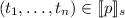
The set $\textsc {T} _S$ of $FO^{++}$ terms of sort S is defined inductively as follows: if x is a variable of sort S then $x\in \textsc {T} _S$; if $f \in \textsc {F}$ has the profile $S_1, \times \ldots \times S_n \rightarrow S$, and for each $i\in 1..n, t_i \in \textsc {T} _{S_i}$ then $f(t_1,\dots ,t_n) \in \textsc {T} _S$. The set $\textsc {T} = \bigcup T_{S_i}$ denotes all $FO^{++}$ terms.

Atoms. The set $\textsc {P}$ of predicate symbols consists of (1) classical predicate symbols, each of which is associated with a profile $S_1,\times \ldots \times S_n$, where n is the arity of the predicate and each $S_i$ is a sort, and (2) two special 2-arity predicates symbols: ${\text {models}}_{\text {LTL}}$ and ${\text {models}}_{\text {CTL}}$. An atom in $FO^{++}$ consists of either a usual predicate applied to $FO^{++}$ terms, or the special predicate ${\text {models}}_{\text {LTL}}$ (resp. ${\text {models}}_{\text {CTL}}$) applied to an $FO^{++}$ term and an LTL (resp. CTL) formula. Considering the latter case, i.e., ${\text {models}}_{\text {LTL}}$ and ${\text {models}}_{\text {CTL}}$, the first argument of both predicates is a term (in practice: a variable representing a function in the source code under analysis). The second argument of ${\text {models}}_{\text {LTL}}$ (resp. ${\text {models}}_{\text {CTL}}$) is an LTL (resp. CTL) formula as defined in Sect. 2.2.

Formulas. $FO^{++}$ formulas are defined as follows: $\top ,\bot$ are formulas, if a is an atom then a is also a formula; if S is a sort and Q is a formula, then $\lnot {Q}, Q \vee Q, Q \wedge Q, Q \iff Q, Q \implies Q, \forall x :S~Q, \exists x:S~Q$ are also formulas.

A sentence is an $FO^{++}$ formula without free-variable. In the rest of the paper, all formulas are sentences.

Semantics

Interpretation Structure. An $FO^{++}$ formula is interpreted over a structure $M = (\mathcal {D}, \mathcal {EKS}, \text {eks}, \mathrm {has\_eks}, I_F, I_P)$. The domain $\mathcal {D}$ is a set in which terms are interpreted. It is partitioned into disjoint sub-domains $\mathcal {D} _S$, one for each sort S; $\mathcal {EKS}$ is a set of Enhanced Kripke Structures ($\textsc {EKS}$) as defined in Sect. 2.2, which are used to interpret temporal formulas. $\mathrm {has\_eks} (x) :\mathcal {D} \rightarrow \{\text {true},\text {false} \}$ is a function, which indicates whether a value in the domain has an associated $\textsc {EKS}$. $\text {eks} :\mathcal {D} \rightarrow \mathcal {EKS}$ is a partial function, which maps some elements of $\mathcal {D}$ to an $\textsc {EKS}$². $I_F$ defines an interpretation for functions in $\textsc {F}$ such that if $f \in \textsc {F}$ has a profile $S_{1}, \times \ldots \times S_{n} \rightarrow S_{n+1}$ then $I_F(f) : \mathcal {D} _{S_{1}}, \times \ldots \times \mathcal {D} _{S_{n}} \rightarrow \mathcal {D} _{S_{n+1}}$. $I_P$ defines an interpretation for predicates in $\textsc {P}$ such that if $p \in \textsc {P}$ has a profile $S_1 \times \ldots \times S_n$ then $I_p(p) \subseteq \mathcal {D} _{S_1} \times \ldots \times \mathcal {D} _{S_n}$ is the set of all tuples of domain values for which p is true.

$I_F$ and $I_P$ are specific to the programming language used for the project under analysis, whereas $\mathcal {D}$ and $\mathcal {EKS}$ are even specific to the program itself.

Environment. An environment is a partial function from the set V of variables to the domain $\mathcal {D}$. If $\sigma$ is an environment, x a variable in V and d a value in $\mathcal {D}$, then $\sigma [x\leftarrow d]$ denotes the environment $\sigma _1$ where $\sigma _1(x)=d$ and for every $x \ne y,\sigma _1(y)=\sigma (y)$.

From an environment $\sigma$ and an interpretation $I_F$ for functions, we define an interpretation $K_{\sigma } : \textsc {T} \rightarrow \mathcal {D}$ for terms in the following way: $\text {for each variable } x \text { in } V, K_{\sigma }(x) = \sigma (x)$ and for an arbitrary term $f(t_1,\dots ,t_n)$, $K_{\sigma }(f(t_1,\dots ,t_n)) = I_F(f)(K_{\sigma }(t_1),\dots ,K_{\sigma }(t_n))$

Satisfaction Rules. Let M be an interpretation structure, $\sigma$ an environment and $K_{\sigma }$ an interpretation for terms according to this environment. We define the satisfaction relation of $FO^{++}$ as follows³:

$$\begin{aligned} \begin{aligned} M,K_{\sigma }&\models \lnot Q \text { iff } M,K_{\sigma } \not \models Q \\ M,K_{\sigma }&\models Q_1\wedge Q_2 \text { iff } M,K_{\sigma } \models Q_1 \text { and } M,K_{\sigma } \models Q_2 \\ M,K_{\sigma }&\models \exists x :S~Q \text { iff } \text {there is an } a \in \mathcal {D} _S \text { such that } M,K_{\sigma [x \leftarrow a]} \models Q \\ M,K_{\sigma }&\models p(t_1,\dots ,t_1) \text { iff } (K_{\sigma }(t_1),\dots ,K_{\sigma }(t_n)) \in I_P(p) \\ M,K_{\sigma }&\models {\text {models}}_{\text {CTL}}(x,\psi ) \text { iff } \mathrm {has\_eks} (x) \text { and } \text {eks} (x),K_{\sigma } \models _{CTL} \psi \\ M,K_{\sigma }&\models {\text {models}}_{\text {LTL}}(x,\psi ) \text { iff } \mathrm {has\_eks} (x) \text { and } \text {eks} (x),K_{\sigma } \models _{LTL} \psi \\ \end{aligned} \end{aligned}$$

If Q is a formula without any free variable, we write $M\models Q$ for $M, K_{\emptyset } \models Q$ where $\emptyset$ denotes an empty environment.

2.2 Temporal Formulas

Syntax. The syntax of LTL and CTL slightly differs from their standard definition, in which atoms are atomic propositions (see, e.g., [19]). Here, since we are in a first-order context, an atom is a predicate in a set $\textsc {PredEKS}$ (disjoint from $\textsc {P}$) applied to terms. We call $\textsc {TAtoms}$ the set of atoms of temporal formulas. The predicates in $\textsc {PredEKS}$ describe syntactic properties of the statements within a CFG (whereas predicates in $\textsc {P}$ denotes (static) structural properties about the source code under study). For instance, in order to reason about the fact the current statement of a CFG contains a call to a certain function, we can define a predicate call($\cdot$) in $\textsc {PredEKS}$, such that call(x) is true if there is a call to the function denoted by the first-order variable x in the current statement of the CFG.

The syntax of LTL is inductively defined as follows: $\textsc {TAtoms}$ are valid LTL formula. If $\psi _1, \psi _2$ are valid LTL formulas, so are $\psi _1 \circ \psi _2$, $\lnot {\psi _1}$, $\mathbf {X}\psi _1$, $\mathbf {G}\,\psi _1$, $\mathbf {F}\,\psi _1$, $\psi _1\mathbin {\mathbf {U}}\psi _2$, $\mathbf {Y}\psi _1$, $\mathbf {O}\,\psi _1$, $\mathbf {H}\,\psi _1$ and $\psi _1\,\mathbin {\mathbf {S}}\,\psi _2$ where $\circ$ is a binary Boolean connective.

CTL syntax is similar to LTL syntax, except that the temporal operators are $\mathbf A \circ {-}$, $\mathbf E \circ {-}$, $\mathbf {A}[-\mathbin {\mathbf {U}}-]$, $\mathbf {E}[-\mathbin {\mathbf {U}}-]$ with $\circ \in \{\mathbf {X},\mathbf {F}\,,\mathbf {G}\,\}$.

Semantics. The slight change of formalism is reflected into the interpretation structures used. Instead of using traditional Kripke structures, $FO^{++}$ uses Enhanced Kripke structures. An Enhanced Kripke structure is simply a Kripke structure where the valuation function associates each state with the interpretation of predicates in $\textsc {PredEKS}$, instead of a set of atomic propositions.

$\textsc {EKS}$ Formal Definition. Let be an $\textsc {EKS}$. S is a set of states, $\rightarrow \subseteq S \times S$ is the transition relation between states (written $\circ \rightarrow \circ$), $I_{_\textsc {EKS}} \subseteq S$ is the set of initial states and associates a predicate p of arity n with its interpretation in a state s, denoted (i.e., the set of all tuples of concrete values for which the predicate is true).

Interpretation Rules for Temporal Formulas. The satisfaction of LTL and CTL formulas is defined in the standard way (see, e.g., [19]), except for atoms, which are built from predicates instead of atomic propositions, as explained above. Given an environment $\sigma$, an interpretation $K_\sigma$, a predicate $p \in \textsc {PredEKS}$, a state s and some terms $v_1,\dots ,v_n$, the satisfaction relation for temporal atoms is defined as follows⁴:

(1)

An example of $FO^{++}$ formula is given in Sect. 4.3.

Remark 1

(Difference with FO-CTL and FO-LTL). Notice that a more classical way of combining first-order and temporal logics results in FO-LTL [15] and FO-CTL [5]. Intuitively, FO-LTL allows a free combination of LTL and first-order symbols and is evaluated on a succession of states on which the value of some variables depends. FO-LTL adds to LTL the possibility to quantify on the values that variables in a given state. FO-CTL is used to specify property on a single first-order Kripke structures. These structures have transitions with conditional assignments and FO-CTL offers to quantify over the variable used in those conditional assignments.

Strictly speaking, we cannot compare their expressive power with respect to $FO^{++}$ because the interpretation structures are different. The main difference is due to the mapping of some domain elements to temporal interpretation structures, which is called $\text {eks}$ in $FO^{++}$ semantics. In $FO^{++}$, a quantification over the elements that are mapped to temporal interpretation structures comes to an indirect quantification over these temporal interpretation structures, which is not possible in the case of FO-LTL and FO-CTL. On the other hand, for pragmatic reasons, we restrict $FO^{++}$ syntax not to allow quantifiers in the scope of temporal operators, whereas they are allowed in FO-CTL and FO-LTL.

3 $FO^{++}$ Model Checking

In this section, we investigate the model checking problem for $FO^{++}$.

3.1 Model Checking Algorithm

Given an $FO^{++}$ formula $\phi$ and an interpretation structure M, the model checking algorithm $\textsc {MC}^{++}(M,\phi )$ returns $\mathtt {true}$ if M satisfies $\phi$, and $\mathtt {false}$ otherwise. To do so, we chose to rely on an approach that is similar to rewriting systems. This way, we can decouple the basic steps of the algorithm (rewriting rules) from the way these steps are ordered (the strategy). This offers a flexible and modular presentation of the algorithm. In our implementation, we also took advantage of this structure to log the different steps of the algorithm for a potential offline review. Notice, however, that we are not strictly in the scope of higher-order rewriting systems such as defined in [18] because some of our rules include conditions that refer to the interpretation structure.

$\textsc {MC}^{++}$ Terms. The terms that are handled by the algorithm $\textsc {MC}^{++}$, called $\textsc {MC}^{++}$ terms, are similar to $FO^{++}$ formulas but include elements of the semantic domain, which are useful for quantifier unfolding. The $FO^{++}$ formula $\phi$ is first translated into an $FO^{++}$ term, which is then successively rewritten until reaching $\mathtt {true}$ or $\mathtt {false}$.

For each sort S, any element $d\in D_S$ is considered as a constant of sort S. Then, if p is a predicate symbol of profile S and $d\in D_S$ is an element of the semantic domain associated with S in M, then p(d) is a valid $\textsc {MC}^{++}$ term. Besides, a quantified formula is represented by a term in which all values that are necessary for the quantifier unfolding are listed. For example, considering a sort S with an associated semantic domain $D_S=\{d_1, \ldots , d_n \}$, the formula $\forall x:s~Q$ is represented by the term $\mathtt {all}_{\textsc {D}}(x.Q, <d_1, \ldots , d_n>)$, and the formula $\exists x:s~Q$ is represented by the term $\mathtt {some}_{\textsc {D}}(x.Q, <d_1, \ldots , d_n>)$.

Rewriting First-Order Terms. The rewriting rules for the first-order part of the logic are split into three categories: the rules related to the evaluation of $FO^{++}$ functions and non temporal predicates, the rules that perform unfolding of quantifiers and the rules that evaluate Boolean connectives.

Functions and Predicates. Functions and predicates are evaluated once all their arguments are domain constants. The values are determined by their respective interpretation functions. The rewriting rules are $p(t_1,\dots t_n) \leadsto \mathtt {true} \text { if }(t_1,\dots ,t_n)\in P(p)$, $p(t_1,\dots t_n) \leadsto \mathtt {false} \text { if }(t_1,\dots ,t_n)\notin P(p)$ and $f(t_1, \dots t_n ) \leadsto I(f)(t_1,\dots ,t_n)$, where each $t_i$ denotes a value in the domain $D_{S_i}$.

Unfolding Quantifiers. Unfolding a universal quantifier (respectively an existential one) transforms the quantified expression x.Q into a conjunction (respectively disjunction) of an expression where the bounded variable x is replaced by a constant d of the domain which has not been considered yet (denoted $Q[x \slash d]$), and the original quantified expression without $d_1$ in the list of values to consider. Quantifiers with an empty list of values are treated in a classical way. Formally, the following four rules are defined:

$\begin{array}{llll} \mathtt {all}_{\textsc {S}}(x.Q,<d,Y>) &{} \leadsto Q[x/d] \wedge \mathtt {all}_{\textsc {S}}(x.Q,<Y>) &{} \mathtt {all}_{\textsc {S}}(x.Q,<~>) &{}\leadsto \mathtt {true} \\ \mathtt {some}_{\textsc {S}}(x.Q,<d,Y>) &{} \leadsto Q[x/d] \vee \mathtt {some}_{\textsc {S}}(x.Q,<Y>) &{}\mathtt {some}_{\textsc {S}}(x.Q,<~>) &{}\leadsto \mathtt {false} \end{array}$

Constant Propagation. Boolean constants $\mathtt {true}$ and $\mathtt {false}$ are propagated upward also in classical manner. And, Or and Imply connectives are evaluated in short-circuit manner from left to right and if short-circuit evaluation is not conclusive, then the term is rewritten into its right subterm. Rules for equivalence connective only applies if both subterms are boolean constants and so do rules for negations.

Rewriting Temporal Predicates. Rewriting a temporal predicate ${\text {models}}_{\text {LTL}}(f,\psi )$ or ${\text {models}}_{\text {CTL}}(f,\psi )$ into a Boolean value is done in two steps:

• 1. a reduction algorithm generates a classical temporal model checking problem out of f and $\psi$;

• 2. the application of a model checking algorithm to this new problem.

Reduction Algorithm. For generating an equivalent model checking problem from ${\text {models}}_{\text {LTL}}(f,\psi )$ or ${\text {models}}_{\text {CTL}}(f,\psi )$ (when f has an $\textsc {EKS}$), the reduction algorithm operates in three steps:

• 1. for each call to a predicate in $\textsc {PredEKS}$ with a unique set of parameters, it generates an atomic proposition. For instance, for $p \in \textsc {PredEKS}$, $t_1 :\mathcal {D},\dots ,t_n :\mathcal {D}$, a call to $p(t_1,\dots ,t_n)$ gives an atomic proposition $id(p,t_1,\dots ,t_n)$. Notice that at this step, because of previous rewriting rules, the parameters of these predicates are necessarily constants (corresponding to values in the domain) and not first-order variables;

• 2. a classical interpretation structure for temporal logic formulas $M_f$ (a transition system, the states of which are labeled with atomic propositions) is built out of $\text {eks}$ (f), the CFG associated with f. The structure of $M_f$ copies the graph from $\text {eks}$ (f), with an extra final state that loops back to itself. For a state s in $\text {eks}$ (f), if , its dual in $M_f$ is labeled with the atomic proposition $id(p,t_1,\dots ,t_n)$;

• 3. the new formula $\phi '$ to analyze over $M_f$ is $\phi$ where each call $p(t_1,\dots ,t_n)$ is substituted by $id(p,t_1,\dots ,t_n)$.

Strategy Used. The algorithm $\textsc {MC}^{++}$ uses a leftmost-outermost strategy to rewrite the formula, which can be described as follows. (1) Try to apply some rule to the toplevel term. (2) If it is not possible then recursively apply the strategy to the leftmost subterm (considered as the new toplevel term), and then (3) try again to apply a rule to the toplevel term. If it is still not possible then apply a rule to the right-hand side subterm.

3.2 Correctness and Termination

In this section, we establish that the algorithm $\textsc {MC}^{++}$ is correct and terminates.

Proposition 1

(Correctness). Let M be an interpretation structure and $\phi$ an $FO^{++}$ formula. If $\textsc {MC}^{++}(M,\phi )$ returns $\mathtt {true}$ then $M \models \phi$, and if $\textsc {MC}^{++}(M,\phi )$ returns $\mathtt {false}$ then $M \nvDash \phi$.

Proof

(sketch). It is straightforward to define a semantics for $\textsc {MC}^{++}$ terms similarly to $FO^{++}$ formulas. Then, we can easily prove that each rewriting rule preserves the semantics of $\textsc {MC}^{++}$ terms. $\square$

Proposition 2

(Termination). Let M be an interpretation structure and $\phi$ an $FO^{++}$ formula. $\textsc {MC}^{++}(M,\phi )$ terminates and returns either $\mathtt {true}$ or $\mathtt {false}$.

Proof

We show that any application of the first-order logic evaluation rules ends (which therefore stands for the chosen strategy). To do so, we consider the following function s as defined in Eq. (2), the value of which decreases with each application of the rules.

$$\begin{aligned} s(\phi ) {\left\{ \begin{array}{ll} (s(\psi ) + 1)^{n+1} &{}\text {if } \phi = \circ (x.\psi ,[d_1,\dots ,d_n]) \text { for } \circ \in \{\mathtt {all}_{\textsc {S}},\mathtt {some}_{\textsc {S}}\}\\ s(\psi _1) + s(\psi _2) &{} \text {if } \phi = \psi _1 \circ \psi _2, \text {for any binary} \circ \text {operator} \\ s(\psi ) + 1 &{} \text {if } \phi = \lnot \psi \\ 1+\sum _{i=1}^n s(d_i) &{} \text {if } \phi = f(d_1,\dots ,d_n),\, f \text { either a function or predicate}\\ 1 &{} \text {otherwise} \\ \end{array}\right. } \end{aligned}$$

(2)

Proof (sketch). For conciseness, we only show the demonstration for the evaluation of functions and predicates (Eq. (3)), as well as for quantifiers unfolding (Eqs. (4) and (5)). Other cases are similar and straightforward. First of all, notices that s is minored by 1.

$$\begin{aligned} \begin{aligned} s(p(d_1,\dots ,d_n)) = 1+\sum \limits _{i=1}^n s(d_i)> 1&= s(\mathtt {false}) = s(\mathtt {true}) \\ s(f(d_1,\dots ,d_n)) = 1+\sum \limits _{i=1}^n s(d_i) > 1&= s(I(f)(d_1,\dots ,d_1)) \end{aligned} \end{aligned}$$

(3)

The second inequality holds because $I(f)(d_1,\dots ,d_1)$ is a constant for the domain and its value by s is 1. By similarity between $\mathtt {all}_{\textsc {S}}$ and $\mathtt {some}_{\textsc {S}}$ for unfolding the quantifiers, we only consider the case of $\mathtt {all}_{\textsc {S}}$.

$$\begin{aligned} \begin{aligned} s(\mathtt {all}_{\textsc {S}}(x.P,<d_1,d2,\dots ,d_n>))&=(s(P)+1)^{n+1} \\&= s(P)(s(P)+1) + (s(P)+1)^n \\&> s(P[x/d_1])+(s(P)+1)^n \\&= s(P[x/d_1] \wedge \mathtt {all}_{\textsc {S}}(x.P,<d_2,\dots ,d_n>)) \end{aligned} \end{aligned}$$

(4)

$$\begin{aligned} \begin{aligned} s(\mathtt {all}_{\textsc {S}}(x.P,<~>))&=(s(P)+1)^{1} > 1 = s(\mathtt {true}) \end{aligned} \end{aligned}$$

(5)

Moreover, generating the equivalent classical temporal model checking problem ends, just as its evaluation with a classical temporal model checking algorithm. This proves that the algorithm ends. Besides, since for every $\textsc {MC}^{++}$ term different from $\mathtt {true}$ and $\mathtt {false}$, some rewriting rule is applicable (this can be proved by induction on $\textsc {MC}^{++}$ terms) then $\textsc {MC}^{++}$ terminates either with $\mathtt {true}$ or with $\mathtt {false}$. $\square$

The completeness directly follows from Proposition 1 and Proposition 2.

Corollary 1

(Completeness). Let M be an interpretation structure and $\phi$ an $FO^{++}$ formula. If $M\models \phi$ then $\textsc {MC}^{++}(M,\phi ) = \mathtt {true}$ and if $M\nvDash \phi$ then $\textsc {MC}^{++}(M,\phi ) = \mathtt {false}$.

3.3 Complexity

Proposition 3

The model checking problem of $FO^{++}$ is PSPACE-complete.

Proof

Hardness: $FO^{++}$ subsumes first-order logic, whose model-checking problem (also called query evaluation) is PSPACE-complete [22]. Hence $FO^{++}$ model-checking is at least as hard as FO model-checking $FO^{++}$ model (i.e. $FO^{++}$ model-checking is PSPACE-hard).

Membership: Let us consider the algorithm $\textsc {MC}^{++}$ presented above with inputs M (an interpretation structure) and $\phi$ (an $FO^{++}$ formula). We consider n as the size of the problem input, i.e., the size of $\phi$ (number of connectives, $FO^{++}$ terms and atoms) plus the size of M (size of the domain, of predicate and function interpretation, plus the number of nodes of the different $\textsc {EKS}$).

The size of the initial $\textsc {MC}^{++}$ term is in O(n). An application of an unfolding rule to an $\textsc {MC}^{++}$ term introduces a larger $\textsc {MC}^{++}$ term and increases the memory space by at most n. Indeed, at most n new memory is required for the new expression ($Q[x \slash d]$ in the unfolding rules). All other rules decrease the memory consumption as they reduce the number of $\textsc {MC}^{++}$ terms. By using the leftmost-outermost strategy and our two unfolding rules the algorithm unfolds the quantifiers in depth-first manner. Let k be the maximum number of nested quantifiers. The algorithm uses at most $(k+1)*n$ space to represent “unfolded” terms before reaching a term where all the first-order variables are substituted by a domain constant. For such a term, the only possible applicable rewriting rules are either the rules for Boolean connectives (which decrease the space needed to represent the term) or the rule for functions and predicates. Functions and non temporal predicates required a constant space to be evaluated. Evaluating temporal predicates is a two steps process. The first step is the reduction algorithm that produces a classical temporal model-checking problem. Its overall size m is smaller than n as both the Kripke structure and the temporal formula mimics the inputs of reduction algorithm and as their respective sizes are components of n. Evaluating this problem is done with a polynomial amount of memory with respect to m (and therefore with respect to n) since model checking for CTL (resp. LTL) is PTIME-complete (resp. PSPACE-complete). Therefore, the space needed for the whole algorithm is polynomial in n, hence the result. $\square$

4 Application to C++ Source Code Analysis

$FO^{++}$ construction remains generic as it does not mention any particular programming language. To be used as a specification language, it must be instantiated for a specific programming language. This means defining appropriate sets for sorts, functions and predicate symbols, as well as a method for extracting an interpretation structure (including interpretation for functions and predicates) from the source code. In this section, we detail the instantiation of $FO^{++}$ for C++.

4.1 $FO^{++}$ for C++

Sort. The sorts indicate the nature of the different structural elements we can reason about. In a C++ program, the different structural elements are declarations such as functions, classes, variables or types. Both classes and types have their own sort. Within functions, we distinguish between free functions and member functions, and operate a further distinction for constructors and destructors. We also operate a distinction on variables between attributes, local variables, and global variables. Hence, $FO^{++}$ for C++ has a total of 9 sorts.

Functions and Non Temporal Predicates. $FO^{++}$ functions are used to designate an element in the code from another related element, such as the unqualified version of a const-qualified type or the class in which an attribute was defined. Non-temporal predicates are used to query information about the structural elements. This includes for instance parenthood relationship between elements (i.e. an attribute a belongs to class c), visibility, inheritance relationship between classes, types and their qualification (const or volatile for instance). The semantics of functions and non-temporal predicates complies with the C++ standard [1]. Table 1 lists some functions and predicates with their informal semantics. The full list of functions and predicates is available on the Pangolin repository⁵.

Table 1. Small subset of structural predicates in the $FO^{++}$ instantiation for C++

4.2 Extracting an Interpretation Structure

Domain. Extracting the domain $\mathcal {D}$ from an AST consists of traversing the AST and collecting the various declarations in order to know the sort of each domain element. Figure 3a shows domain $\mathcal {D}$ obtained from the source code shown in Listing 1.1, partitioned into four sub-domains (one for each relevant sort).

Fig. 3.

Semantic domain partially illustrated

Generating $\mathcal {EKS}$ . If the full definition of a C++ function f is present in the AST of the C++ source code, then $\mathrm {has\_eks} (f)$ is true and $\text {eks} (f)$ is defined in the following manner. We consider the CFG of f, where each node only contain a single statement (a basic block is not included into a node, but is split into a succession of nodes instead). The $\textsc {EKS}$ states and transitions of $\text {eks} (f)$ are then directly taken from the nodes and edges of the CFG of f, except that the state corresponding to the exit node of the CFG has an infinite loop on itself to ensure infinite traces and comply with LTL and CTL semantics. Function calls are considered like any other statement, hence there is neither interprocedural analysis nor specific recursive calls handling. In each state of the $\textsc {EKS}$, the valuation of the predicates in $\textsc {PredEKS}$ directly follows from the syntax of the statement that is in this state. Notice that some paths of the $\textsc {EKS}$ may never be taken by the program execution, because, e.g., a condition of a while loop is always evaluated to false during execution. Since we do not perform value analysis, our method still considers such paths. This is in accordance with our objective to analyze the quality of the code, instead of checking its semantic correctness.

Figure 3b shows the $\textsc {EKS}$ for serB with two elements from $\textsc {PredEKS}$: $call$, and $assign$. The predicate $call(x)$ is true on states such that there is a call to function x (the arguments do not matter) and $assign (x)$ is true on states such that there is an assignment to x (i.e. $x = \dots$).

4.3 Example: Formalizing Log Correct Usage

To illustrate concretely $FO^{++}$ for C++, we formalize Property 1 in Eq. (6). The universal quantification on c indicates that the property applies to all classes. We then look for a private attribute l whose type is Log. (The symbol Log is here an $FO^{++}$ constant.) We then look at all attributes of class c, and if there is one whose type is Log, then we look for a function s such that

• Each private attribute a from class c (whose type is not Log) is logged in s (i.e. there is a call to log on l with a as argument in s). The formalization of this relies on the predicate $call\_log$ of $\textsc {PredEKS}$ such that $call\_log(x,y)$ is true on a CFG state if there is call of the shape x.log(y) in this state. The CTL formula $\mathbf {AF} call\_log(l,a)$ states that in all paths within the CFG of s, there is finally a state in which $call\_log(l,a)$ is true.

• For all public functions f, in all paths in the CFG of f, there is at some point a call to s, and the attribute a is no longer assigned after this call.

$$\begin{aligned} \begin{aligned}&\forall c :\textsc {class} ~\forall l :\textsc {attr} ~\big ( isAttributeOf (l,c) \wedge type (l,Log) \implies \\&\exists s:\textsc {memfct} ~( isMemFctOf (s,c) \wedge name (s,\texttt {store}) \wedge \\&\forall a :\textsc {attr} ~( isAttributeOf (a,c) \wedge isPrivate (a) \wedge \lnot type (a,\texttt {Log}) \implies \\&~~~~~~~~~~{\text {models}}_{\text {CTL}}(s,\mathbf {AF} call\_log(l,a) ) \wedge \\&\forall f:\textsc {memfct} ~( isMemFctOf (f,c) \wedge isPublic (f) \implies \\&~~~~~~~~~~{\text {models}}_{\text {CTL}}(f, \mathbf {AF} call (s) \wedge \mathbf {AG} ( call (s) \implies \mathbf {AX}\mathbf {AG} \lnot assign (a)) ))))\big ) \end{aligned} \end{aligned}$$

(6)

5 Pangolin

Pangolin⁶ is a verification engine for C++ programs based on the ideas developed in Sects. 2 to 4. Given a rule as a formula in $FO^{++}$ for C++, Pangolin checks whether the specification holds on the program. Figure 4 illustrates this process as well as some of the internal aspects of Pangolin.

Fig. 4.

Pangolin overview

From the user point of view, the specification is written in a concrete syntax of $FO^{++}$ for C++ as it is presented in Sect. 4.1. The code to analyze must compile in order to be examined as Pangolin needs to traverse the code AST to extract an $FO^{++}$ interpretation structure. This implies that a simple extract of code taken out of its context cannot be analyzed. For each formula and each file, Pangolin returns true if the formula holds on the file and false otherwise. It also prints a complete trace of the evaluation process that can be reviewed. If the formula does not hold, it is possible to find with this trace the values of the quantified variables that explain algorithm output, hence providing a counter-example. It also increases the user’s confidence in the correctness of the implementation.

From an internal point of view, Pangolin consists of two parts: an interpretation structure extractor and a model checking engine. The extractor follows the specification given Sect. 4.2, and is based on Clang and its API libtooling [17]. Clang provides an up-to-date and complete support for C++, direct access to the code AST and facilitates the computation of the CFG of a function. Pangolin implements the model checking algorithm presented in Sect. 3, and it relies on nuXmv [9] for evaluating model checking problems resulting from the reduction algorithm. However, because of short-circuit evaluation of logical connectives, the model-checking algorithm stops at the first counter-example found. With this algorithm, to find the next counter-example, it is necessary either to change the formula to exclude the counter-example that was found, or to correct the code and then start over the analysis. To find all the possible counter-examples, Pangolin also implements an alternative algorithm where quantifiers are unfolded less efficiently, so that all the values for the different quantifiers are explored, which makes it possible to find all the counter-examples at once.

6 Experiments

We study the conformity of two open-source projects with respect to six generic properties that address good programming practices accepted for C++. The first project is ZeroMQ, a high-performance asynchronous messaging framework. The second is MiniZinc [21], a solver agnostic modeling language for combinatorial satisfaction and optimization problems. We picked these two projects because they are active popular C++ projects with a middle size code base (around 50k SLOC each).

6.1 Properties to Test

Table 2 lists the six properties we want to verify on ZeroMQ and Minizinc. P1 mainly ensures that the version of a function that can be executed from anywhere in a class hierarchy is unambiguous, hence bringing clarity for maintainers and reviewers. Rule P2 forbids to mix into a single class virtual functions and overloaded arithmetic operators. Indeed, a class with virtual functions is meant to be used in polymorphic context. But it is difficult to write foolproof and useful arithmetic operators that behave coherently in a polymorphic context.

P3 ensures that there no unused private elements (function and attributes) within a class. Indeed, they are only accessible from within the class, and unused private elements are either superfluous (and hindering code quality) or symptom of a bug. P4 must be enforced because the C++ programming language specifies that virtual function resolution is not performed within constructors and destructors. Hence, when there is a call to a virtual function in either the constructors or destructors, the callee is likely not to be the intended function.

The last two rules are to enforce const-correctness. The driving idea behind the const correctness is to prevent the developer from modifying by accident a variable or an object because it would result in a compilation error. Variables marked as const are immutable whereas const member functions cannot alter the internal state of an object. Thus, any non-constant element must be justified: a variable assigned at most once must be constant (P5), and objects with only calls to constant member functions must also be constant as well (P6).

For the sake of conciseness, we only show (in Eq. (7)) the formal translation of property P5⁷. The rule uses the word modified, whose meaning must be specified by the formalization. Here, we say that a variable x is modified when it is to the left of a binary operator (i.e. x $= where $ is (eventually) one operator among , +, -, , *, $\mathtt { \& }$, $\mathtt {|}$, $\texttt {<<}$, $\texttt {>>}$) or is the argument of an unary operator among increment, decrement or addressof (i.e. x++, ++x, x–, –x, $\mathtt { \& x}$). For clarity, in Eq. (7), $modified (x)$ is an abbreviation for a disjunction of 15 predicates (one for each operator). Also, the formalization is done in a “negative” way: we look for a function f in which a not constant variable v is modified at least once (the first $\mathbf {AF} \dots$ part) and never again afterwards $\mathbf {AG} \dots \implies \mathbf {AX}\mathbf {AG} \lnot {\dots }$.

Table 2. Properties to verify

$$\begin{aligned} \begin{aligned} \exists f&:\textsc {FreeFct} \Big ( \exists v :\textsc {LocalVar} \big ( locallyDeclared (v,f) \wedge \lnot { isConst (v)} \wedge \\&{\text {models}}_{\text {CTL}}(f, \mathbf {AF} modified (v) \wedge \mathbf {AG} ( modified (v) \implies \mathbf {AX}\mathbf {AG} \lnot { modified (v)}))\big )\Big ) \end{aligned} \end{aligned}$$

(7)

6.2 Results and Analysis

Table 3 summarizes the experiments on ZeroMQ and MiniZinc. For each rule and each project, columns CE shows the total number of counter-examples found and column Timing the average time over 10 runs with its standard deviation, both in seconds.

Table 3. Summary of the defects found in ZeroMQ and MiniZinc with the average required time to perform the analysis

Defects Found. For property P1, all counter-examples found are real violations of the rule. Pangolin found no counter-example for property P2. Regarding P3, Pangolin found for ZeroMQ 3 unused attributes and 1 for MiniZinc. Many of the functions that Pangolin found, many were, in fact, called. Two were virtual and inherited from a parent class but with reduced visibility as it is allowed by C++. They were therefore called from a function of the parent class. The rest of the functions were used but not as specified. For instance, they were used as callbacks or called on an object of the same type as the class (this is allowed in C++ because between 2 objects of the same type, there is no encapsulation). Concerning P4, Pangolin found one counter-example on MiniZinc, which was a true violation. Many of the results for rules P5 and P6 are real counter-examples for the specification but are legitimate code. Indeed, for P5 does not take into account that a variable may change through a pointer or a reference, while rule P6 does not take into account public attributes of a class that may change.

With hindsight, these false alarms could have been removed with a more precise rule. For instance, for property P6, there two approaches to design a more precise rule. On the one hand, one could exclude classes with public attributes from the property (i.e. in all functions, any locally declared object whose class does not have public attributes and on which only const member functions are called must also be marked as constant). On the other hand, one could into account the public attributes for determining if an object should be constant (In all functions, any locally declared object on which only const member functions are called and no public attributes are changed must also be marked as constant).

Performance. The tests were performed on Intel(R) Xeon(R) CPU E5-1607 v3 @ 3.10 GHz with 32 GB of memory. Properties involving temporal properties are slower than sheer structural properties. Indeed, there is an overhead to evaluate temporal predicates. This overhead is the sum of the time spent to evaluate of the classical model-checking problem on the one hand and of communication time on the other hand. The former varies with the complexity of the formula and of the $\textsc {EKS}$, whereas the latter is constant. The execution time of P5 and P6 is radically different between the 2 projects (despite a comparable size) because a particular Minizinc function contains more than 3000 lines and temporal predicates are long to evaluate over it. This shows that Pangolin can scale and find defects in real code bases.

7 Related Work

There are many existing code representations and associated formalisms to specify queries. A more detailed comparison of existing code query technologies can be found in [2] or in [11]. ASTLOG [10] is a project for examining directly a program AST with a Prolog-based language. Thus, it allows to directly examine the very structure of the AST, whereas our approach exploits the AST to gain information and does not directly analyze it. In [20], the authors generate UML models from the AST of the code and use Object Constraint Language [7] to perform queries. HERCULES/PL [14] is a pattern specification language for C and Fortran programs on top of the HERCULES framework. It uses the target language and HERCULES specific compiler annotations (such as pragma in C) for specifying the code to match. In [12], the authors define TGraphs, a graph representation of the whole AST of the program, and they define GReQL, a graph querying language for performing queries. QL [4] uses a special relational database that contains a representation of the program extracted from its AST. Queries are expressed in a programming language similar to SQL, and are compiled to Datalog. Like all these methods (expect ASTLOG), our method works with a code representation that is built from the AST outside the functions. However, unlike all the above-mentioned methods, in addition to the AST, our approach also examines the body of functions through paths within their CFG, and allows for sophisticated reasoning about these paths through temporal logics.

On the other hand, Coccinelle [6] focuses on the CFG of a C function instead of its AST. It uses CTL-VW (a variant of FO-CTL) to describe and retrieve a sequence of statements within a CFG. This reasoning about execution paths within a CFG was an inspiration for the temporal aspect of $FO^{++}$. But, unlike Coccinelle, $FO^{++}$ can specify a property about several functions through the first-order reasoning over the code AST. However, Coccinelle has a code transformation feature, which $FO^{++}$ does not offer.

In [13], the authors detect design patterns described in formalism based on a combination of predicate logic and Allen’s interval-based temporal logic. The complete formalism is latter translated into Prolog to effectively search the design pattern. However, its semantic model is not provided (especially how functions are handled). $FO^{++}$ offers a more modular combination mechanism for logics and integrates two discrete temporal logics (CTL and LTL), which we think are more natural to use than the Allen’s temporal logic, given that the statements are discrete events.

8 Conclusion

This paper presents a formal approach to source code verification in which the requirements can simultaneously refer to execution paths in the CFG of functions and to structural information that comes from the source code AST. To formalize the requirements, we introduce the logic $FO^{++}$, which is a temporal extension of many-sorted first-order logic. We propose a model checking algorithm for $FO^{++}$ and prove its correctness, termination and that $FO^{++}$ model checking problem is PSPACE complete. This approach has been implemented in Pangolin, a tool for analyzing C++ programs. With it, we analyzed two middle-sized open-source projects (ZeroMQ and MiniZinc), looking for violations of 6 good-practice coding-rules and found several occurrences of them.

As future works, there are two directions: user interaction, and expressive power. An input language closer to real code and better user feedback would improve user interaction. The expressive power of the method would be increased with interprocedural and multi-file analysis and the adequate specification formalism to handle it.

References

ISO International Standard ISO/IEC 14882:2014(E) Programming Language C++
Alves, T.L., Hage, J., Rademaker, P.: A comparative study of code query technologies. In: Proceedings - 11th IEEE International Working Conference on Source Code Analysis and Manipulation, SCAM 2011, pp. 145–154 (2011)
Alves, T.L., Visser, J.: Static estimation of test coverage. In: 2009 Ninth IEEE International Working Conference on Source Code Analysis and Manipulation, pp. 55–64, September 2009
Avgustinov, P., De Moor, O., Jones, M.P., Schäfer, M.: QL: object-oriented queries on relational data. In: Ecoop 2016, pp. 1–25 (2016)
Bohn, J., Damm, W., Grumberg, O., Hungar, H., Laster, K.: First-order-CTL model checking. In: Arvind, V., Ramanujam, S. (eds.) FSTTCS 1998. LNCS, vol. 1530, pp. 283–294. Springer, Heidelberg (1998). https://doi.org/10.1007/978-3-540-49382-2_27
Brunel, J., Doligez, D., Hansen, R.R., Lawall, J.L., Muller, G.: A foundation for flow-based program matching. ACM SIGPLAN Not. 44(1), 114 (2009)
Cabot, J., Gogolla, M.: Object Constraint Language (OCL): a definitive guide. In: Bernardo, M., Cortellessa, V., Pierantonio, A. (eds.) SFM 2012. LNCS, vol. 7320, pp. 58–90. Springer, Heidelberg (2012). https://doi.org/10.1007/978-3-642-30982-3_3
Caleiro, C., Sernadas, C., Sernadas, A.: Parameterisation of logics. In: Fiadeiro, J.L. (ed.) WADT 1998. LNCS, vol. 1589, pp. 48–63. Springer, Heidelberg (1999). https://doi.org/10.1007/3-540-48483-3_4
Cavada, R., et al.: The nuXmv symbolic model checker. In: Biere, A., Bloem, R. (eds.) CAV 2014. LNCS, vol. 8559, pp. 334–342. Springer, Cham (2014). https://doi.org/10.1007/978-3-319-08867-9_22
Crew, R.F.: ASTLOG: a language for examining abstract syntax trees. In: Proceedings of the Conference on Domain-Specific Languages on Conference on Domain-Specific Languages (DSL), DSL 1997, p. 18. USENIX Association, Berkeley (1997)
Dit, B., Revelle, M., Gethers, M., Poshyvanyk, D.: Feature location in source code: a taxonomy and survey. J. Softw. Evol. Process. 25(1), 53–95 (2013)
Ebert, J., Bildhauer, D.: Reverse engineering using graph queries. In: Engels, G., Lewerentz, C., Schäfer, W., Schürr, A., Westfechtel, B. (eds.) Graph Transformations and Model-Driven Engineering. LNCS, vol. 5765, pp. 335–362. Springer, Heidelberg (2010). https://doi.org/10.1007/978-3-642-17322-6_15
Huang, H., Zhang, S., Cao, J., Duan, Y.: A practical pattern recovery approach based on both structural and behavioral analysis. J. Syst. Softw. 75(1–2), 69–87 (2005)
Kartsaklis, C., Hernandez, O.R.: HERCULES/PL: the pattern language of HERCULES. In: Proceedings of the 1st Workshop on Programming Language Evolution, pp. 5–10 (2014)
Kuperberg, D., Brunel, J., Chemouil, D.: On finite domains in first-order linear temporal logic. In: Artho, C., Legay, A., Peled, D. (eds.) ATVA 2016. LNCS, vol. 9938, pp. 211–226. Springer, Cham (2016). https://doi.org/10.1007/978-3-319-46520-3_14
Lawall, J.L., Muller, G., Palix, N.: Enforcing the use of API functions in Linux code. In: Proceedings of the 8th Workshop on Aspects, Components, and Patterns for Infrastructure Software - ACP4IS 2009, p. 7 (2009)
Lopes, B.C., Rafael, A.: Getting Started with LLVM Core Libraries (2014)
van Raamsdonk, F.: Higher-order rewriting. In: Narendran, P., Rusinowitch, M. (eds.) RTA 1999. LNCS, vol. 1631, pp. 220–239. Springer, Heidelberg (1999). https://doi.org/10.1007/3-540-48685-2_17
Huth, M., Ryan, M.: Logic in Computer Science (2004)
Seifert, M., Samlaus, R.: Static source code analysis using OCL. Electron. Commun. EASST 15 (2008)
Stuckey, P.J., Feydy, T., Schutt, A., Tack, G., Fischer, J.: The MiniZinc challenge 2008–2013. AI Mag. 35(2), 55–60 (2014)
Vardi, M.Y.: The complexity of relational query languages (extended abstract). In: Proceedings of the Fourteenth Annual ACM Symposium on Theory of Computing, STOC 1982, pp. 137–146. ACM, New York (1982)
Author information
Authors and Affiliations
Corresponding author
Editor information
Editors and Affiliations
Rights and permissions
Copyright information
© 2018 Springer Nature Switzerland AG
About this paper
Cite this paper
Come, D., Brunel, J., Doose, D. (2018). Source Code Analysis with a Temporal Extension of First-Order Logic. In: Massoni, T., Mousavi, M. (eds) Formal Methods: Foundations and Applications. SBMF 2018. Lecture Notes in Computer Science(), vol 11254. Springer, Cham. https://doi.org/10.1007/978-3-030-03044-5_3
Download citation
DOI: https://doi.org/10.1007/978-3-030-03044-5_3
Published:
Publisher Name: Springer, Cham
Print ISBN: 978-3-030-03043-8
Online ISBN: 978-3-030-03044-5
eBook Packages: Computer ScienceComputer Science (R0)