Single-Degree-of-Freedom Oscillator

Abstract

Single-degree-of-freedom oscillators are often found as such in musical acoustics. It is important to understand their behavior because they are elementary building blocks of more complicated (discrete or continuous) systems in the context of the modal theory. In this chapter, a number of basic results are summarized. Fundamental methods, based on the use of Green’s functions, are introduced and applied to the harmonic oscillator. Their relevance and efficiency for treating more complex systems will appear throughout this book. Whenever possible, conclusions are drawn concerning practical examples. Two important notions, that are not always intuitively well understood by musicians, are addressed: resonance and reverberation. In addition, three different definitions of the quality factor are given, and the analysis of the harmonic oscillator in terms of energetic quantities is emphasized.

These keywords were added by machine and not by the authors. This process is experimental and the keywords may be updated as the learning algorithm improves.

1 Introduction

For this introductory chapter, the most common example of a standard mechanical oscillator is chosen. We have seen how to switch from mechanical to acoustical resonators by means of analogies (see Table 1.1). The example of the Helmholtz resonator without dissipation, in particular, has been studied in Chap. 1 (Sect. 1.5). Consider a mechanical oscillator of mass M, stiffness K, and with a viscous damping coefficient R, driven by a force f(t) and whose moving part has a velocity v(t) (see Fig. 2.1). The motion of this oscillator is described by the differential equation:

$$\displaystyle{ M \frac{dv} {dt} + Rv + K\int vdt = f, }$$

(2.1)

which can be written equivalently with respect to displacement y(t) ($v(t) = dy(t)/dt$) and usual scaled parameters:

$$\displaystyle{ \frac{d^{2}y} {dt^{2}} + 2\alpha _{0}\frac{dy} {dt} +\omega _{ 0}^{2}y = \frac{f} {M}, }$$

(2.2)

where

$$\displaystyle{ \omega _{0}^{2} = \frac{K} {M}\quad \text{and}\quad \alpha _{0} =\zeta _{0}\omega _{0} = \frac{\omega _{0}} {2Q_{0}} = \frac{R} {2M}. }$$

(2.3)

Fig. 2.1

Single-degree-of-freedom mechanical oscillator

The resonance angular frequency is denoted by ω ₀, which, because of the damping coefficient R, is not necessarily equal to the eigen (or natural) angular frequency: both angular frequencies will be defined later in this chapter. Q ₀ is the second basic parameter describing the sharpness of the resonance: it is called “quality factor,” and plays an essential role in several properties of the oscillator. One should remember that its limit is infinite when damping approaches zero. It may appear cumbersome to define three quantities to express damping, α ₀, ζ _o , and Q ₀. However, each quantity has its own meaning and use, as it will be seen later.

The damping model has not been discussed yet. In Chap. 5 it will be shown that damping often depends on frequency, which of course strongly modifies the time-domain equation (2.2). It is assumed that it is not the case here. Similarly, the damping coefficient is chosen positive so that free oscillations decrease exponentially: in fact, for self-oscillating instruments (see Part III), the sound starts with an exponential growth, because the energy source is proportional to the term R, which can be either positive or negative.

2 Solution With and Without a Source: Green’s Function

2.1 Solution Without a Source; Eigenfrequency

The first step is to write the solutions of Eq. (2.2) without source terms, i.e., after the extinction (f(t) = 0). This corresponds therefore to the case of free oscillations. Complex solutions in the form Ae ^{j ω t} are sought, where ω is the angular eigenfrequency.¹ The equation to be solved is derived from Eq. (2.2):

$$\displaystyle{ \left [ \frac{\omega } {\omega _{0}}\right ]^{2} - j \frac{1} {Q_{0}} \frac{\omega } {\omega _{0}} - 1 = 0, }$$

(2.4)

and the solutions are given by:

$$\displaystyle{ \omega _{0}^{\pm } = j\alpha _{ 0} \pm \omega _{p}\;\text{where}\;\omega _{p} =\omega _{0}\delta _{0},\ \ \text{with }\delta _{0} = \sqrt{1 -\zeta _{ 0 }^{2}} = \sqrt{1 - \frac{1} {4Q_{0}^{2}}}. }$$

(2.5)

If ζ ₀ is greater or equal to unity, i.e., if Q ₀ is lower or equal to 1∕2, the two solutions $\omega _{0}^{\pm }$ are purely imaginary, and there is no oscillations. Discarding this case, two complex eigenfrequencies are found, which have the same real part ω _p , in absolute value. The real part is often called (angular) eigenfrequency of the oscillator, even if the signal is pseudo-periodic, when it is attenuated. In the following, the term “eigenfrequency” will be used for $\omega _{0}^{+}$ and $\omega _{0}^{-}$ as well as for ω _p , because there is generally no ambiguity. The general solution is written as:

$$\displaystyle{ y(t) = e^{-\alpha _{0}t}\left [A^{+}e^{j\omega _{p}t} + A^{-}e^{-j\omega _{p}t}\right ]\;\text{ or }\;y(t) = Ae^{-\alpha _{0}t}\sin (\omega _{ p}t+\varphi ). }$$

(2.6)

The first expression involves two complex coefficients, A ^±, but only the real part is of interest for us. The second expression involves two real coefficients: A and $\varphi$. The signal has a pseudo-period $T = 2\pi /\omega _{p}$, and is exponentially attenuated, the exponent being proportional to ζ ₀. During a pseudo-period, the amplitude of the signal is divided by a factor:

$$\displaystyle{ e_{T} =\exp \left [-\text{}\frac{2\pi } {\delta _{0}} \zeta _{0}\right ] =\exp \left [- \frac{\pi } {Q_{0}\delta _{0}}\right ]\text{. } }$$

(2.7)

The larger the quality factor, the longer the oscillation. If it is large enough ($\delta _{0} \simeq 1$), an approximate definition for the oscillation to decrease by a factor e = 2. 7 is given by the number of pseudo-periods, divided by π. Table 2.1 gives some typical values of quality factors encountered in some musical instruments.

Table 2.1 Some typical values of the quality factor Q in musical acoustics

The coefficients A and $\varphi$ in (2.6) can be found provided that initial values of the function y(t) and its first derivative v(t) are known. The following results are obtained by setting t = 0 in Eq. (2.6) and in the corresponding expression for dy∕dt:

$$\displaystyle{ y(t) = e^{-\alpha _{0}t}\left [\frac{1} {\omega _{p}}\left [v(0) +\alpha _{0}y(0)\right ]\sin \omega _{p}t + y(0)\cos \omega _{p}t\right ], }$$

(2.8)

and

$$\displaystyle{ v(t) = e^{-\alpha _{0}t}\left [v(0)\cos \omega _{ p}t -\delta _{0}^{-1}\left [\zeta _{ 0}v(0) +\omega _{0}y(0)\right ]\sin \omega _{p}t\right ]. }$$

(2.9)

A special case of initial conditions, which is important for future considerations, is the case where the oscillator is released without initial velocity and with an initial displacement y(0). This means that a force $f^{-}(t) = F^{-} = Ky(0)$ was applied during negative time. The velocity (see Fig. 2.2) is expressed by:

$$\displaystyle{ v(t) = -\frac{F^{-}} {M\omega _{p}}e^{-\alpha _{0}t}\sin (\omega _{ p}t). }$$

(2.10)

Fig. 2.2

Oscillator released at t = 0 without initial velocity. On the left the displacement and on the right the velocity. y(0) = 1; f ₀ = 30 Hz; Q ₀ = 18. 85. In this case it takes 6 pseudo-periods for the oscillation to decrease by a factor e

and the displacement:

$$\displaystyle{ y(t) = y(0)e^{-\alpha _{0}t}\left [\cos (\omega _{ p}t) + \frac{\zeta _{0}} {\delta _{0}}\sin (\omega _{p}t)\right ] = \frac{y(0)} {\delta _{0}} e^{-\alpha _{0}t}\cos (\omega _{ p}t+\varphi ) }$$

(2.11)

where $\tan \varphi = -\zeta _{0}/\delta _{0}$ (or $\cos \varphi =\delta _{0}).$

2.2 Solution with an Elementary Source: Green’s Function

Expression (2.11) is a first illustration of an oscillator with a source switched off at t = t ₀. Looking also at negative times, it can be written as a solution of the following equation, with a source term:

$$\displaystyle{ \frac{d^{2}y} {dt^{2}} + 2\alpha _{0}\frac{dy} {dt} +\omega _{ 0}^{2}y = \frac{F^{-}} {M} H(t_{0} - t), }$$

(2.12)

where H(t) is the Heaviside step function. The velocity is a solution of the following equation:

$$\displaystyle{ \frac{d^{2}v} {dt^{2}} + 2\alpha _{0}\frac{dv} {dt} +\omega _{ 0}^{2}v = -\frac{F^{-}} {M} \delta (t - t_{0}). }$$

It is therefore, to within the multiplicative factor $-F^{-}/M$, a solution of the equation with an elementary source δ(t − t ₀). The solution is called Green’s function. This function and its first derivative are assumed to be equal to zero at time t < t ₀. It allows expressing a solution for any source (see the following section). The Green’s function is denoted g(t | t ₀), and is a solution of the following equation:

$$\displaystyle{ \left [ \frac{d^{2}} {dt^{2}} + 2\alpha _{0} \frac{d} {dt} +\omega _{ 0}^{2}\right ]g(t\vert t_{ 0}) =\delta (t - t_{0}), }$$

(2.13)

and, according to (2.10), is equal to:

$$\displaystyle{ g(t\vert t_{0}) = \frac{1} {\omega _{p}}H(t - t_{0})e^{-\alpha _{0}(t-t_{0})}\sin [\omega _{ p}(t - t_{0})]. }$$

(2.14)

t ₀ is the pulse emission time, and t is the observation time. Note that the Green’s function is a function of (t − t ₀): it does not change if the emission time t ₀ is changed to − t, and the observation time from t to − t ₀. This is the property of temporal reciprocity. ² Except for a multiplying factor, its shape is that of the velocity in Fig. 2.2, if t ₀ = 0.

A direct solution of Eq. (2.13) is now shown. To simplify the problem it is assumed that t ₀ is zero. The method is similar to the one developed for the solution without a source (2.8), by matching solutions at t = 0. It is known that, for t > 0, the solution has the form (2.6). Both coefficients A and $\varphi$ are found by matching this solution to the solution for negative time, which is equal to zero, as it is the case for its first derivative. It can be shown, and at least it can be a posteriori checked, that the presence of the Dirac delta function in Eq. (2.13) implies the continuity of the solution at t = 0, hence $\varphi = 0$, and the discontinuity of its first derivative. By integrating Eq. (2.13) between $t-\varepsilon$ and $t+\varepsilon$, the following results are obtained:

$$\displaystyle{ \left [ \frac{d} {dt}g(t,0)\right ]_{t-\varepsilon }^{t+\varepsilon } = 1\;\text{ hence }\;A = \frac{1} {\omega _{p}}\,, }$$

and Eq. (2.14) is obtained again for t ₀ = 0.

2.3 General Solution with a Source Term

2.3.1 Solution by Fourier Transform

From the Green’s function, the general equation (2.2) can be solved. We first derive the Fourier transforms of the equation with y(t) and of the Green’s function equation:

$$\displaystyle\begin{array}{rcl} \left [-\omega ^{2} + 2\alpha _{ 0}j\omega +\omega _{ 0}^{2}\right ]\mathcal{Y}& =& \frac{F} {M}{}\end{array}$$

(2.15)

$$\displaystyle\begin{array}{rcl} \left [-\omega ^{2} + 2\alpha _{ 0}j\omega +\omega _{ 0}^{2}\right ]G& =& 1{}\end{array}$$

(2.16)

where $\mathcal{Y}(\omega )$, F(ω), and G(ω) are the Fourier transforms of y(t), f(t), and g(t | 0). Calculating the ratio of the two previous equations yields

$$\displaystyle{ \mathcal{Y}(\omega ) = \frac{F(\omega )} {M} G(\omega ). }$$

(2.17)

Therefore, by returning to the time domain, and considering that the convolution product is the inverse Fourier transform of the ordinary product in the frequency domain, we get

$$\displaystyle\begin{array}{rcl} y(t)& =& \frac{1} {2\pi M}\int _{-\infty }^{+\infty }F(\omega )G(\omega )e^{j\omega t}d\omega = \frac{1} {M}\int _{-\infty }^{+\infty }f(t^{{\prime}})g(t - t^{{\prime}}\vert 0)dt^{{\prime}}, \\ \text{or }y(t)& =& \frac{1} {M}\int _{-\infty }^{+\infty }f(t^{{\prime}})g(t\vert t^{{\prime}})dt^{{\prime}} = \frac{1} {M}\int _{-\infty }^{t}f(t^{{\prime}})g(t\vert t^{{\prime}})dt^{{\prime}}. {}\end{array}$$

(2.18)

In fact, because the Green’s function $g(t\vert t^{{\prime}})$ is a function of $(t - t^{{\prime}})$, the convolution becomes a simple product, and the Green’s function is equal to zero for $t^{{\prime}} > t$.

2.3.2 Solving by Laplace Transform

For a source starting at a given time, the force can be written $f(t) = H(t)\tilde{f}(t)$, and the previous result (2.18) is applicable. But it is often more convenient to use the Fourier transform of the product rather than the convolution product. It is then easier to use the Laplace transform, which involves the initial conditions [see Eq. (1.118)]. Equation (2.17) is replaced by:

$$\displaystyle{ \mathcal{Y}(s) = G(s)\left [F(s)/M + (s + 2\alpha _{0})y(0) + v(0)\right ] }$$

(2.19)

and the integral equation (2.18) becomes

$$\displaystyle{ y(t) = \frac{1} {M}\int _{0}^{t}f(t^{{\prime}})g(t\vert t^{{\prime}})dt^{{\prime}} + \left [2\alpha _{ 0}y(0) + v(0)\right ]g(t\vert 0) + y(0)\frac{dg(t\vert 0)} {dt}. }$$

(2.20)

If there is no source f(t), the solution without a source (2.8) is found again, which can be verified.³

3 Examples of Free and Forced Oscillations

This section aims at studying some examples of solutions, in the case of a steady-state excitation, or for an excitation which is either starting or stopping at a given time. One can easily imagine a vibrating string, acting as an oscillating source for a sound box that would have a single-degree-of-freedom: the starting and stopping of the sound box’s vibration is of great interest, even if the present study will provide qualitative results only. Similarly one can easily transpose these simple situations to any instrument producing a sound in a room: it also acts as an oscillating source. This illustration implies that the oscillation produced is not influenced by the room itself; this is reasonable, except maybe in the case of an organ (because of the size of the pipes).

3.1 Displacement of a System from Equilibrium

We first treat the case of the displacement of a system from equilibrium, because it is very simple and complementary to the case of a system released without initial velocity [Eq. (2.11)]. Let the force be f(t) = F _M H(t), the system being at equilibrium at t = 0: y(0) and v(0) are zero. We do not discuss the method for producing such a force. We can use the linearity of the problem, and therefore the superposition principle, and observe that $f(t) + f^{-}(t) = F_{M}$, if $f^{-}(t) = F_{M}H(-t)$, which is a case we have already described in Eq. (2.11). Now the solution for f(t) = F _M (constant) is known: it is $y(t) = F_{M}/M\omega _{0}^{2}$. Subtracting the solution (2.11) from this result, we obtain the complete solution:

$$\displaystyle{ y(t) = \frac{F_{M}} {M\omega _{0}^{2}}\left [1 - e^{-\alpha _{0}t}\left (\cos (\omega _{ p}t) + \frac{\zeta _{0}} {\delta _{0}}\sin (\omega _{p}t)\right )\right ]. }$$

(2.21)

The expected initial conditions are satisfied. However, we find that it was not needed to use them for this new problem! In fact all the information is contained in the evolution of the force from $t = -\infty$ to $+\infty$: f(t) = F _M H(t). The important fact is that a sudden change of excitation in one direction or the other produces a free oscillation which is attenuated exponentially, in addition to the steady term F _M ∕M ω ₀ ² (see Fig. 2.3).

Fig. 2.3

Displacement of the system from equilibrium: the displacement is calculated with the same parameters as in Fig. 2.2, but y(0) = 0

3.2 Excitation (Forced) by a Steady Sinusoidal Force

Consider, for example, $f(t) = F_{M}\cos \omega t$. The solution is the real part of the solution for f(t) = F _M e ^{j ω t}. For steady forced oscillations, the solution can be sought in the form A(ω)e ^{j ω t}. The derivatives are then derived in a straightforward way. The oscillating response has the same frequency as the excitation. Now, the eigenfrequency intervenes in the amplitude only: this point will be discussed in detail later. Using Eq. (2.16), one obtains

$$\displaystyle{ y(t) = F_{M}M^{-1}G(\omega )e^{j\omega t}. }$$

(2.22)

Taking the real part of this result yields

$$\displaystyle\begin{array}{rcl} y(t) = \frac{F_{M}} {M} \mathfrak{R}e\left [ \frac{e^{j\omega t}} {-\omega ^{2} + 2j\alpha _{0}\omega +\omega _{ 0}^{2}}\right ] = \frac{F_{M}} {MD^{1/2}(\omega )}\sin (\omega t+\varphi )& &{}\end{array}$$

(2.23)

where

$$\displaystyle\begin{array}{rcl} D(\omega ) = \left [(\omega ^{2} -\omega _{ 0}^{2})^{2} + 4\alpha _{ 0}^{2}\omega ^{2}\right ]\text{; }\tan \varphi = (-\omega ^{2} +\omega _{ 0}^{2})/2\alpha _{ 0}\omega.& &{}\end{array}$$

(2.24)

The velocity is given by:

$$\displaystyle{ v(t) = A\cos (\omega t+\varphi )\text{ where }A = \frac{\omega F_{M}} {MD^{1/2}(\omega )}. }$$

(2.25)

3.3 Excitation by a Sinusoidal Force Starting at t = 0

Consider now the particular case when the starting time of the source is taken into account. Let us roughly suppose that it starts abruptly: the force is, for example, $f(t) = F_{M}H(t)\cos \omega t$. We now calculate the velocity by using the Laplace Transform. The transform of the force is $F(s) = F_{M}s/(s^{2} +\omega ^{2})$, and that of the derivative is $F_{M}s^{2}/(s^{2} +\omega ^{2}) - f(0^{+}) = -F_{M}\omega ^{2}/(s^{2} +\omega ^{2})$. Since the initial velocity and the acceleration are zero (velocity is zero for all negative times), the transform of the velocity is

$$\displaystyle{ V (s) = -\frac{F_{M}} {M} \frac{\omega ^{2}} {(s^{2} +\omega ^{2})(s^{2} + 2\alpha _{0}s +\omega _{ 0}^{2})}. }$$

(2.26)

The standard method for calculating the inverse transform is the partial fractions expansion in terms of the form $(s - s_{n})^{-1}$, which leads to simple poles. It is actually more efficient to group the conjugate poles (we expect to find the combination of two signals of angular frequency ω and ω _p ). We are therefore looking to write V (s) as:

$$\displaystyle{ V (s) = \frac{as + b} {s^{2} +\omega ^{2}} + \frac{a^{{\prime}}s + b^{{\prime}}} {s^{2} + 2\alpha _{0}s +\omega _{ 0}^{2}}. }$$

(2.27)

The result is obtained, after identification and inverse transform, but the calculation remains heavy. A lighter approach is based on the observation that, given the form of Eq. (2.27), the solution is of the type:

$$\displaystyle{ v(t) = H(t)\left [A\cos (\omega t+\varphi ) + A_{p}e^{-\alpha _{0}t}\cos (\omega _{ p}t +\varphi _{p})\right ], }$$

(2.28)

and thus only the first term remains when time goes to infinity. In other words, the first term is equal to the solution (2.25), multiplied by H(t). To find the other two parameters, we can simply use the initial conditions (zero velocity and acceleration), which gives

$$\displaystyle{ \omega \tan \varphi =\alpha _{0} +\omega _{p}\tan \varphi _{p}\text{; }A\cos \varphi = -A_{p}\cos \varphi _{P}, }$$

and, after some calculations, $A_{p} = A\omega /\omega _{p}$.

The second term in the right-hand side of (2.28) is not negligible compared to the first as long as the observation period is small compared to the characteristic damping time $\alpha _{0}^{-1}$. For some weakly damped structural modes of musical instruments, this characteristic time can be of the order of magnitude of 0.1 ms or higher. Therefore, assuming that the exponential becomes negligible after a time of five to ten times larger, it appears that this second term cannot be neglected for 0.5 to 1 s after the excitation has started, if we want to correctly estimate the average power dissipated.

3.4 Excitation by a Sinusoidal Force Stopping at t = 0

What happens for a force stopping at t = 0, i.e., $f(t) = F_{M}H(-t)\cos \omega t$? One can use the Fourier Transform, with the necessary precautions concerning the function H(−t), but a simpler method exists. We use the principle of superposition applied to the previous problem, which gives a sinusoidal steady source, and we derive by simple subtraction between (2.25) and (2.28):

$$\displaystyle{ v(t) = AH(-t)\cos (\omega t+\varphi ) - A_{p}H(t)e^{-\alpha _{0}t}\cos (\omega _{ p}t +\varphi _{p}). }$$

(2.29)

The form (2.29) is interesting because it exhibits the reverberation: after the pulsation source ω stops, the oscillator vibrates at its eigenfrequency, with free oscillations. The phenomenon that occurs when the source starts [see Eq. (2.28)] can also be called reverberation: however, it overlaps with the oscillation produced by the source. The reverberation is a phenomenon triggered by the non-stationarity of a source: it is an oscillation whose frequency is the eigenfrequency of the system, and which decreases because of damping. These results are qualitatively very general, since they can be extended to any vibrating system with several degrees of freedom (DOF). The only phenomenon that cannot occur with a single DOF (i.e., a single mode) is the phenomenon of echo, due to delays: in a room, there is a very large number of modes (or DOF), which combine together and produce successive reflections on the walls. In Chap. 4 the relationship between modes and waves will be presented.

4 Forced Oscillations: Frequency Response

Forced sinusoidal motions are often used in experimental devices, in order to estimate the mechanical losses of a structure, in particular. It is therefore necessary to understand their main aspects and their theoretical limitations. In a steady sinusoidal regime, it is convenient to use the complex notation, what we adopt hereafter. We wish to study the response of the displacement (Eq. 2.15), and, above all, the velocity due to a sinusoidal force $f(t) = F_{M}\exp (j\omega t)$, since the product of force by velocity determines the power. We must therefore consider the response, called mechanical admittance, when the frequency varies

$$\displaystyle{ Y (\omega ) = \frac{V (\omega )} {F(\omega )} = \frac{1} {M} \frac{j\omega } {-\omega ^{2} + 2j\omega \alpha _{0} +\omega _{ 0}^{2}}, }$$

(2.30)

the Fourier Transform of f(t) being $F(\omega ^{{\prime}}) = F_{M}\delta (\omega ^{{\prime}}-\omega )$. A function of ω of this form is often called “Lorentzian.” We are interested in the quantities: modulus, argument (which is a phase difference), real and imaginary parts of the admittance, for which the evolution versus frequency can be seen in Figs. 2.4 and 2.5. We limit the study to the response in velocity, because in musical acoustics the input admittance (or impedance) is the most useful response. However the responses in displacement or in acceleration are interesting too, and show other variations with frequency.

Fig. 2.4

Oscillator’s admittance modulus and argument versus frequency, for Q ₀ = 18. 85; f ₀ = 30 Hz, M = 1

Fig. 2.5

Real (dotted line) and imaginary part (solid line) of the oscillator’s admittance versus frequency, for Q ₀ = 18. 85; f ₀ = 30 Hz, M = 1

It will be shown in Chap. 3 that for any discrete or continuous system, under certain conditions, the response is simply the sum of quantities of the type (2.30), each corresponding to a mode. For forced oscillations, we are interested in the maximum of this quantity; for self-sustained oscillations, our interest is in the zeros of the imaginary part (this will be explained in Chap. 9), the two kinds of frequencies being very close. For the present case (single mode), they are identical.

To study the admittance variation versus frequency, the easiest way is to start by considering the inverse quantity, i.e., the impedance

$$\displaystyle{ Z(\omega ) = j\omega M + R + \frac{K} {j\omega } = M\omega _{0}\left [j \frac{\omega } {\omega _{0}} - j\frac{\omega _{0}} {\omega } + \frac{1} {Q_{0}}\right ]. }$$

(2.31)

Z is real when ω = ω ₀, which implies that the admittance also is real. For ω > ω ₀, the leading term is the mass term, otherwise it is the stiffness term $M\omega _{0}^{2}/j\omega$. The real parts of Z and Y are always positive for a passive system, as explained in Chap. 1. The imaginary part is either positive or negative.

The modulus Z is minimum when ω = ω ₀, the so-called resonance angular frequency. For a given amplitude of excitation F (the cause), it corresponds to the angular frequency for which the amplitude of the response V (the effect) is maximum.⁴ It differs from the angular eigenfrequency ω _p , unless the damping is low [large Q ₀, see Eq. (2.5)]. If Q ₀ is large, impedance and admittance are almost purely imaginary at any frequency, except very close to the resonance.

Two other frequencies are interesting⁵: these are those for which the imaginary part is equal or opposite to the real part (the argument of Z is then ±π∕4). This gives the following values:

$$\displaystyle{ \frac{\tilde{\omega }^{\pm }} {\omega _{0}} = \sqrt{1 + \frac{1} {4Q_{0}^{2}}} \pm \frac{1} {2Q_{0}} = 1 \pm \frac{1} {2Q_{0}} + O\left ( \frac{1} {Q_{0}^{2}}\right ). }$$

(2.32)

For very large Q ₀, they are very close to the resonance frequency. It is easy to show that they correspond to extrema of the imaginary part of admittance, which can be written as:

$$\displaystyle{ Y = \frac{1} {M\omega _{0}}Q_{0} \frac{1 - j\mu Q_{0}} {1 +\mu ^{2}Q_{0}^{2}}\text{ where }\mu = \frac{\omega } {\omega _{0}} -\frac{\omega _{0}} {\omega }. }$$

(2.33)

At these frequencies, the modulus of Y is thus equal to its value at the resonance (μ = 0), divided by $\sqrt{2}$. We note that

$$\displaystyle{ \frac{\tilde{\omega }^{+} -\tilde{\omega }^{-}} {\omega _{0}} = \frac{1} {Q_{0}}\sqrt{1 + \frac{1} {4Q_{0}^{2}}}. }$$

(2.34)

This quantity is the relative width of the peak of the quantity $\left \vert Y \right \vert ^{2}$ at half maximum: for large Q ₀, it is close to 1∕Q ₀. This is a second definition of the quality factor, the first one being the decay rate by period for free oscillations [see (2.7)]. However the two definitions only coincide at the third order of Q ₀ ⁻¹. We still have to examine the variation of the real part of the admittance: Equation (2.33) shows that it reaches a maximum at the resonance, and it is then equal to:

$$\displaystyle{ \mathfrak{R}e(Y ) = \left \vert Y \right \vert = \frac{Q_{0}} {M\omega _{0}} = \frac{1} {R}. }$$

(2.35)

4.1 Remarks on the Determination of the Resonance Frequency

We notice that the resonance frequency ω ₀ does not depend on the quality factor. This is why in the case where we are only interested in resonance frequencies, the quality factor can be taken to be infinite, i.e., the damping equal to zero. We then have a purely imaginary admittance, which approaches $\pm \infty$ when the frequency approaches the resonance. In this case, the shape of the curve of the imaginary part of Y becomes very different, since the two extrema are infinite, and it does not cross 0 (Fig. 2.6). If we consider Eq. (2.33), we see that the limit of the imaginary part of Y when $Q_{0}\longrightarrow \infty$ is not straightforward for small μ. On the other hand, the modulus of the impedance Z shows little change.

Fig. 2.6

Imaginary part of the admittance when Q ₀ tends to infinity: there is no zero-crossing. The dotted curve represents the case Q ₀ = 18. 85. The two curves merge far from resonances

It turns out that the imaginary part of the impedance is a very good candidate for determining the resonance frequency by interpolation. A simple calculation shows that if $\mathfrak{I}m(Z)$ is known at two angular frequencies ω ₁ and ω ₂, the resonance is given by:

$$\displaystyle{ \omega _{0}^{2} = \frac{\omega _{1}\omega _{2}\left [\omega _{2}\mathfrak{I}m(Z_{1}) -\omega _{1}\mathfrak{I}m(Z_{2})\right ]} {\omega _{1}\mathfrak{I}m(Z_{1}) -\omega _{2}\mathfrak{I}m(Z_{2})}. }$$

(2.36)

This method can be used even if other modes are present, since the admittance is then the sum of terms of type (2.33). In the presence of modes, some of them may have an amplitude such that the imaginary part of Y does not vanish anymore. Nevertheless if we ignore the damping terms, each term goes to infinity at resonance, and this problem does not arise. Ignoring damping to find the resonance frequencies is therefore very usual and this approximation is very useful in musical acoustics, regardless of the number of modes. Finally, what happens when damping, and therefore the quality factor depends on frequency (in this case, the initial time-domain equation can be greatly modified)? If we look at the cancelation of the imaginary part, the resonance frequency remains independent of the variation of damping with frequency, as seen in the expression of the impedance (2.31). Conversely if we look at the maximum of the modulus of Y for forced oscillations, it is a bit more complicated but it can be shown that the variation of Q ₀(ω) leads to a variation of magnitude 1∕Q ₀ ² only, for both the resonance frequency and the⁶ maximum.

Simplification of the response around the resonance: “simple” modesWe saw in Sect. 2.2.1 that a single-degree-of-freedom oscillator has two complex eigenfrequencies denoted $\omega _{0}^{\pm }$ [Eq. (2.5)]. These frequencies are the (simple) poles of the admittance (2.30). We have

$$\displaystyle{ \omega ^{2} - j\omega \omega _{ 0}/Q_{0} -\omega _{0}^{2} = (\omega -\omega _{ 0}^{+})(\omega -\omega _{ 0}^{-}). }$$

Hence if $Y _{M0} = Q_{0}/M\omega _{0}$ is the maximum of the modulus of Y:

$$\displaystyle{ Y = \frac{1} {M} \frac{j\omega } {\omega _{0}^{2} -\omega ^{2} + j\omega \omega _{0}/Q_{0}} = -\frac{j} {2} \frac{Y _{M0}} {Q_{0}\delta _{0}} \left [ \frac{\omega _{0}^{+}} {\omega -\omega _{0}^{+}} - \frac{\omega _{0}^{-}} {\omega -\omega _{0}^{-}}\right ]. }$$

(2.37)

Each term can be seen as a mode that we will call “simple mode.” Around $\omega =\omega _{0}$, we can ignore the term of negative eigenfrequency (more specifically the term with a negative real part), which gives, if $Z_{m0} = 1/Y _{M0}$ is the minimum of the impedance:

$$\displaystyle\begin{array}{rcl} Z=1/Y \simeq 2jQ_{0}\delta _{0}Z_{m0}\left [\frac{\omega -\omega _{0}^{+}} {\omega _{0}^{+}} \right ]= \frac{1} {1+j/(2Q_{0}\delta _{0})}Z_{m0}\left [1+2jQ_{0}\frac{\omega -\omega _{0}\delta _{0}} {\omega _{0}} \right ].& & \\ & &{}\end{array}$$

(2.38)

If the quality factor Q ₀ is large enough, this reduces to:

$$\displaystyle{ Z \simeq Z_{m0}\left [1 + 2jQ_{0}\frac{\omega -\omega _{0}} {\omega _{0}} \right ] \simeq 2jZ_{m0}Q_{0}\frac{\omega -\omega _{0}^{+}} {\omega _{0}}. }$$

(2.39)

This highlights that such an approximation is convenient for representing a Lorentz resonance near its maximum, at the cost of a first-order approximation in 1∕Q ₀. A more direct approximation method is to write $\omega =\omega _{0}(1+\varepsilon )$ in Eq. (2.37) and expand it to the first order in $\varepsilon$. This approximation is justified as well as the truncation of a modal series to a single mode, under the condition that the frequency is close to the resonance of this mode, with a high quality factor.

5 Energy, Power, and Efficiency

5.1 Energy and Power

The instantaneous mechanical power p _m (t) of the oscillator is given by the scalar product of f and v (see Chap. 1), which leads to:

$$\displaystyle{ p_{m} = \frac{d} {dt}\left [\frac{1} {2}Mv^{2} + \frac{1} {2}Ky^{2}\right ] + Rv^{2}. }$$

(2.40)

The three terms on the right-hand side of (2.40) represent the temporal variations of the kinetic energy of mass M, the elastic energy of spring K, and the power dissipated in the resistance R, respectively.

In most applications, the time average of p _m (t), i.e., its slow fluctuations, is more interesting than its fine details and rapid evolution in time. In audible acoustics, for instance, the human ear is sensitive to the sound level which is well correlated to the average value of the sound power, after integration over a period of 50 ms. This is typically the kind of information that can be read on a sound level meter. In room acoustics, the reverberation time is defined in the same way as the decay of the slow fluctuations of the energy density in the room after the excitation has stopped.

We define below an integration time T whose selection criteria will be discussed later. Using Eq. (2.40) we calculate the average mechanical power $\mathcal{P}_{m}(T)$:

$$\displaystyle{ \mathcal{P}_{m}(T) = \frac{1} {2T}\left [Mv^{2}(T) + Ky^{2}(T) - Mv^{2}(0) - Ky^{2}(0)\right ] + \frac{1} {T}\int _{0}^{T}Rv^{2}(t)dt. }$$

(2.41)

For free oscillations the average power $\mathcal{P}_{m}(T)$ is zero. We derive

$$\displaystyle{ \frac{1} {2}\left [Mv^{2}(T) + Ky^{2}(T)\right ] = \frac{1} {2}\left [Mv^{2}(0) + Ky^{2}(0)\right ] -\int _{ 0}^{T}Rv^{2}(t)dt, }$$

(2.42)

which quantifies the average power $\mathcal{P}_{s}(T) =\int _{ 0}^{T}Rv^{2}(t)dt$ dissipated during the given time interval T. This power $\mathcal{P}_{s}(T)$ is also the power needed by the system to ensure a periodic motion of period T. We notice, in this case, that the quantity between brackets in (2.41) vanishes.

5.1.1 Special Case: Steady Sinusoidal Movement

For an excitation force $f(t) = F_{M}\cos \omega t$, it has been shown in Eq. (2.25) that the velocity is given by $v(t) = V _{M}\cos (\omega t+\varphi )$. Therefore, the average power is written as follows:

$$\displaystyle{ \mathcal{P}_{m}(T) = \frac{1} {T}\int _{0}^{T}F_{ M}V _{M}\cos \omega t\cos (\omega t+\varphi )dt }$$

(2.43)

The oscillation period is denoted $\tau = \tfrac{2\pi } {\omega }$. The integration time is then given by $T = n\tau +\tau _{o}$, where n is a positive integer. The average power becomes

$$\displaystyle{ \mathcal{P}_{m}(T) = \frac{1} {2}F_{M}V _{M}\cos \varphi + \frac{F_{M}V _{M}} {4(2\pi n +\tau _{o}\omega )}\left [\sin (2\omega \tau _{o}+\varphi )-\sin \varphi \right ]. }$$

(2.44)

5.1.1.1 Discussion

• Equation (2.44) shows that the average power $\mathcal{P}_{m}(T)$ is approximately equal to $\frac{1} {2}F_{M}V _{M}\cos \varphi$ only if the average integration period involves a sufficiently large number n of oscillation periods. For the special case where T equals τ, the equality is strict. In what follows, we consider that this condition is satisfied, so that the dependence of the terms of the average power on the integration period is suppressed.

• For a given force, the expression of the velocity was found (see Sect. 2.3.2). The average power can be written using complex quantities:

  $$\displaystyle{ \mathcal{P}_{m} = \frac{1} {2}\mathfrak{R}e\left [f(t)v^{{\ast}}(t)\right ] = \frac{1} {2}F_{M}^{2}\mathfrak{R}e(Y ). }$$

  (2.45)

  This result, which is consistent with Eq. (1.131), confirms the well-known result that the maximum of dissipated power is obtained when the excitation frequency is equal to the resonance frequency of the oscillator, namely for ω = ω ₀. Then, following Eq. (2.35) we can write:

  $$\displaystyle{ \mbox{ Max}\left \{\mathcal{P}_{m}\right \} = \frac{F_{M}^{2}} {2R} . }$$

  (2.46)

• As a consequence, from Eq. (2.46), if F _M is known, we can easily derive R by power measurements.

• For forced oscillations with angular frequency ω, the calculation of the power $\mathcal{P}_{m}$ exhibits terms in ω +ω ₀ δ ₀ and $\left \vert \omega -\omega _{0}\delta _{0}\right \vert$, where δ ₀ is defined in Eq. (2.5). Consequently, the average power exhibits low frequency variations before the steady state emerges (see Fig. 2.7). Experimentally, this transient state may take some time if ω is close to ω ₀, which might pose some difficulty for practical measurements of the average power.

  Fig. 2.7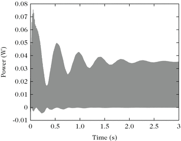

  

  Variation with time of the average dissipated power for an excitation angular frequency ω close to the angular eigenfrequency ω ₀

5.1.2 Third Definition of the Quality Factor

It is possible to link the average power supplied to the energy of the system, averaged over a period, through the quality factor Q ₀. The total energy, which is the sum of kinetic energy and potential energy, is given in Eq. (2.40). Using complex quantities for force and velocity, we have $f(t) = F_{M}\exp (j\omega t)$ and $v(t) = V _{M}\exp (j\omega t+\varphi )$. Using the results of Chap. 1, the power and the total energy averaged over a period are given by:

$$\displaystyle{ \mathcal{P}_{m} = \frac{1} {2}R\left \vert v\right \vert ^{2}\text{ et }\mathcal{E} = \frac{1} {4}\left [M\left \vert v\right \vert ^{2} + K\left \vert y\right \vert ^{2}\right ]. }$$

We get the ratio

$$\displaystyle{ \frac{\mathcal{E}} {T\mathcal{P}_{m}} = \frac{\omega } {4\pi } \frac{M\left \vert v\right \vert ^{2} + K\left \vert y\right \vert ^{2}} {R\left \vert v\right \vert ^{2}} = \frac{Q_{0}} {4\pi } \frac{\omega } {\omega _{0}}\left [1 + \frac{\omega ^{2}} {\omega _{0}^{2}}\right ]. }$$

This shows that at the resonance, it is equal to Q ₀∕2π. This definition complements the definitions based on the decay rate (2.7) and on the relative width of the resonance peak (2.34). These three definitions coincide for small damping values only. When a more general response is considered, expressed as the sum of several modes, the situation becomes even more complicated. Finally, at the resonance, the average energy is equally distributed between potential and kinetic energy.

5.2 Mechanical Air Loaded Oscillator

The following example is the simplest model of acoustic radiation by a structure with a single-degree-of-freedom. As in the previous paragraph, we examine its properties in terms of energy, and we define its efficiency in terms of power.

To illustrate the model, imagine a mechanical single-degree-of-freedom oscillator loaded by a semi-infinite tube of cross section S, filled with air of density ρ and where the sound speed is denoted c (see Fig. 2.8). A wave travels in the tube whose specific characteristic impedance ρ c was found in Chap. 1 (Sect. 1.2.4). The pressure force is simply proportional to velocity. The equation of this oscillator is written as:

$$\displaystyle{ f\!=\! M \frac{dv} {dt} + Rv + K\int vdt + R_{a}v\quad \mbox{ with}\quad R_{a} =\rho cS. }$$

(2.47)

The instantaneous power supplied to the system is written as follows:

$$\displaystyle{ p_{m}(t) = \frac{d} {dt}\left [\frac{1} {2}Mv^{2} + \frac{1} {2}Ky^{2}\right ] + (R + R_{ a})v^{2}. }$$

(2.48)

Hence the average power (per period) is

$$\displaystyle{ \mathcal{P}_{m}(T) = \frac{1} {T}\int _{0}^{T}Rv^{2}(t)dt + \frac{1} {T}\int _{0}^{T}R_{ a}v^{2}(t)dt = \mathcal{P}_{ s}(T) + \mathcal{P}_{a}(T), }$$

(2.49)

Fig. 2.8

Mechanical single-degree-of-freedom oscillator loaded by air

where $\mathcal{P}_{a}(T)$ is the average acoustic power radiated into the tube. We define the acoustical efficiency by:

$$\displaystyle{ \eta = \frac{\mathcal{P}_{a}(T)} {\mathcal{P}_{m}(T)} = \frac{\mathcal{P}_{a}(T)} {\mathcal{P}_{s}(T) + \mathcal{P}_{a}(T)} = \frac{R_{a}} {R + R_{a}}. }$$

(2.50)

This last result requires some comments.

• We observe in (2.50) that the efficiency is independent of T.

• Although the form of η here appears to be very simple, its experimental determination is not straightforward because it requires to estimate R, for example, through measurements in vacuo.

• In the academic example presented above, R _a is obtained analytically, which is rarely the case for structures with complex materials and geometry such as musical instruments. In the general case, $\mathcal{P}_{a}(T)$ is obtained experimentally (or numerically) by computing the flow of the acoustic intensity vector over a closed surface surrounding the source.

• In general, the efficiency may depend on frequency, which is not the case here, but when there are no losses (this corresponds here to setting R = 0) it is always, by definition, equal to unity! Conversely, we have seen that the response of a resonant system always depends on frequency, especially when the losses are small (see, for example, Fig. 2.4). Efficiency and response are therefore quantities whose physical meaning is very different.

5.2.1 Link Between Radiated Power and Damping Factor

For a radiating single-degree-of-freedom system, it is possible to estimate the sound power from the measurement (or numerical simulation) of the damping factor, in free oscillations. In Chap. 13, we will examine the conditions for extending this result to systems with multiple DOF. The equation of the mechanical oscillator loaded by air can be written in a reduced form:

$$\displaystyle{ \frac{d^{2}y} {dt^{2}} + 2\zeta \omega _{0}\frac{dy} {dt} +\omega _{ 0}^{2}y = 0\ \ \ \mbox{ with}\ \ \ \zeta = \frac{R + R_{a}} {2M\omega _{0}}, }$$

(2.51)

for which it is known that the solution is written as (assuming ζ < 1):

$$\displaystyle{ y(t) =\exp (-\zeta \omega _{0}t)\left [\cos (\omega _{0}\sqrt{1 -\zeta ^{2}}t) + \frac{\zeta } {\sqrt{1 -\zeta ^{2}}}\sin (\omega _{0}\sqrt{1 -\zeta ^{2}}t)\right ]. }$$

(2.52)

Equation (2.52) shows that the damping factor (equal to the inverse of the time constant) is equal to:

$$\displaystyle{ \alpha =\zeta \omega _{0} = \frac{R + R_{a}} {2M} . }$$

(2.53)

In conclusion, considering the definition (2.3), we note that, for the simple case of a single-degree-of-freedom oscillator, the acoustical efficiency can be estimated in the time domain by using the expression:

$$\displaystyle{ \eta = \frac{\alpha -\alpha _{0}} {\alpha } . }$$

(2.54)

Note It should, however, be emphasized that one of the damping effects is to slightly modify the frequency of the oscillator, compared to the in vacuo case. This effect has no consequence here because, concerning a “monochromatic” signal, the determination of α from the exponential envelope is independent of the oscillation frequency. Furthermore, in the present example, the air load is considered as purely resistive. If, however, we are in a situation where the fluid load also includes a mass or elastic component, we could not obtain the efficiency from a formula as simple as Eq. (2.54). This point of view will be developed in more detail in Chap. 13.