Radiation of Complex Systems

Abstract

The fundamental properties of the constitutive elements of musical instruments were presented in the previous chapters: vibrating systems, holes, and air columns. Some fundamental coupling situations between such elements, as well as their radiation in free space were also described. In this last chapter, a detailed presentation of some selected instruments is given (vibraphone, timpani, guitar, and piano). In the previous approach made on simple systems, one goal was to give a general view on several order of magnitudes for the involved physical quantities, in order to identify general laws in terms of time, space, and frequency. Here, a complementary point of view is adopted: the geometry, material and frequency range of a given instrument are fixed, and the interaction between its elements is examined for this particular configuration. The objective is to build a complete model of an instrument and to study the vibratory and acoustical phenomena from the initial excitation (mallet impact, struck or plucked string) to the acoustic radiation. The modeling complexity of these sound sources is due to several causes: complex structural geometry, coupling between different components with distinct mechanical properties, broad frequency range, and required accuracy. Finally, the previous presentation of wind instruments is supplemented here by the analysis of radiation by both the tone holes and apertures, and by the resulting interferences.

These keywords were added by machine and not by the authors. This process is experimental and the keywords may be updated as the learning algorithm improves.

1 Example of the Vibraphone

1.1 Introduction

The vibraphone belongs to the family of mallet percussion instruments , as the xylophone , the marimba , and the glockenspiel [47]. All these instruments work in a similar way: horizontal beams are excited by the impact of a mallet and radiate sound. In most cases, a tubular resonator is put under each beam. The function of such resonators is to capture a fraction of the sound energy radiated by the beam and, in turn, to radiate again after amplification and filtering of some frequencies. The instruments of this family differ from each other both by their geometry (size) and material. A vibraphone is made of metallic beams, whereas marimba and xylophone beams are usually made of wood. The case of the vibraphone, which is presented here, can be generalized to the other mallet instruments.

From the point of view of radiation, the vibraphone is a typical example of interaction between a field radiated by an impacted beam and a tubular resonator placed in its vicinity (see Fig. 14.1).¹

Fig. 14.1

Left: vibraphone (Courtesy of Rythmes et Sons). Right: schematic representation of a vibraphone beam and tube. The pressure at point $M(r,\theta )$ is the sum of the pressure radiated by the beam and the pressure radiated by the open end of the tube at a distance r _T

In Chap. 1, the flexural equations of motion for an Euler–Bernoulli beam were presented. The eigenmodes were calculated in Chap. 3, for beams of constant and variable sections. The damping mechanisms in both the tubes and beam materials were presented in Chap. 5 Here, the radiation of the complete instrument is described. According to the usual geometry and materials of the instrument, the following simplifying assumptions are made:

• 1. The vibrations of the beam are not affected by the radiated field. It has been shown in the previous chapters that this assumption is reasonable, as long as the ratio between air and material density is small and, in addition, for a sufficiently rigid beam, as it is the case here. This amounts to assuming that the coefficient $\varepsilon$ in Eq. (13.67) is small compared to unity.

• 2. The transverse dimension (width) b of the beam is small compared to the acoustic wavelength: kb ≪ 1. For a typical beam of width b = 3 cm, this yields an upper limit of 11 kHz for the frequency. In most mallet instruments, the spectral energy is below this limit, except for the highest notes of the xylophone. In what follows, this condition is assumed to be fulfilled, so that some approximations can be made for calculating the radiated pressure field, according to the results presented in Chap. 12.

• 3. The radiation of the tube, at its open end, is not affected by the presence of the beam. It has been shown experimentally that this assumption remains valid as long as the end-beam distance remains small: d∕b ≫ 1. Otherwise, the eigenfrequencies of the tube might be modified, due to the change in the boundary conditions [25].

• 4. Only the flexural vibrations of the beam contribute to the radiation significantly. This is almost true in practice, except if the impact is located near the corners. In this latter case, additional torsional vibrations are generated. These vibrations are generally unpleasant and unwanted, since they are not in harmonic relationships with the flexural modes. In what follows, it is thus assumed that the vibraphone is struck by a talented player who is able to control the impact point of the mallets with precision! Denoting y ₀ the distance between the symmetry axis of the beam and the impact point, the condition y ₀∕b ≪ 1 is assumed (see Fig. 14.2).

  Fig. 14.2

  

  Excitation of the beam near the symmetry axis, in order to avoid the generation of torsional waves (y ₀ ≪ b)

• 5. Finally, it is assumed that the diameter D of the tube is sufficiently small so that only the longitudinal modes exist. This is true under the condition $D/\lambda \ll 1$, where $\lambda$ is the acoustic wavelength (see Chap. 7). It is also admitted that the walls of the tube are rigid and do not contribute to the radiation.

The physical behavior of the vibraphone can be summarized as follows (see Fig. 14.3):

Fig. 14.3

Physical principles of the vibraphone. The beam radiates due to the impact of the mallet. A part of the radiated field excites the air column in the tubular resonator. The resonator radiates, in turn, a sound field where its own eigenfrequencies are dominant in the spectrum. The beam-tube coupling is efficient only if the tube is tuned so that some of its eigenfrequencies are close to the eigenfrequencies of the beam (see Fig. 14.4)

• The impact of the mallet induces flexural vibrations in the beam . The excited eigenfrequencies are close to those of a beam with free boundary conditions. The suspension of the beam by a cord can be viewed as a flexible spring, so that the eigenfrequency of the oscillator made of the complete beam mass and the cord is equal to a few Hz, and thus is far below the first flexural mode. This rigid-body mode is very weakly coupled to the flexural modes, and does not radiate sound.

• From the point of view of radiation, the oscillating beam can be viewed as a linear array of dipoles (see the next section).

• A fraction of the acoustic energy radiated by the beam is captured by the tubular resonator. This resonator acts as an acoustic filter. Only the spectral components of the input field which are close to the eigenfrequencies of the tube can persist. The other components are subject to destructive interferences inside the tube, and are attenuated progressively.

• A fraction of the acoustic energy stored in the tube is radiated to the external field through the open end. The resonator thus acts as a secondary source. An observer in space receives the pressure contributions of both the beam and tube. The spectral content of the tube pressure is dominated by the eigenfrequencies of the tube: the amplitude of these components is significant only if some of the input components (the eigenfrequencies of the beam ) coincide with some eigenfrequencies of the tube: the tube is then said to be tuned to the beam (see Fig. 14.4).

  Fig. 14.4

  

  Basic principles of tuning between a beam and a tubular resonator. (a) shows the spectral content of a tuned beam where the three first flexural modes are tuned to f ₁, 4f ₁, and 10f ₁, respectively. (b) shows the spectrum of a tube closed at one end and open at the other, for which only the odd harmonics exist. It can be seen on this example that the beam and the tube are tuned if both fundamental frequencies are equal. The upper harmonics of the beam do not excite the tube

1.2 Radiation of the Beam

If the acoustic wavelength $\lambda$ is large compared to the width b of the beam, then the reflection of waves radiated by the beam on its surface is negligible. As a consequence, it has been shown in Chap. 12 that the monopolar terms can be neglected in the Kirchhoff–Helmholtz integral (12.61). The only remaining terms are the dipolar terms due to the oscillation of the beam [34]. The total field radiated by the beam is then the sum of elementary dipoles distributed along its length L. A discrete formulation of this sum is given below. Each elementary dipole has a width $\varDelta x = L/N$, where N is the number of elements, length b, and thickness h(x) (see Fig. 14.5).

Fig. 14.5

Decomposition of the beam into an equivalent linear array of elementary oscillating spheres

In order to benefit from simple known results, it is convenient to represent each element of the beam by an equivalent oscillating sphere. This is achieved by considering each element as a sphere with identical volume. The error made by using such an approximation becomes noticeable when the acoustic wavelength is less than or equal to Δ x, which corresponds here to typically 1–5 mm. The radius a(x) of the equivalent sphere is given by:

$$\displaystyle{ \frac{4} {3}\pi a^{3}(x) = bh(x)\varDelta x =\varDelta V (x), }$$

(14.1)

where x ∈ [0, L]. Under the assumptions of far field, as seen in Chap. 12, the field radiated by each equivalent oscillating sphere is written in the time domain [see Eq. (12.40)]:

$$\displaystyle\begin{array}{rcl} \varDelta p[r(x),\theta (x),t]& =& \frac{3\rho \varDelta V (x)\cos \theta (x)} {8\pi r(x)} \\ & & \times \left [ \frac{1} {r(x)}\gamma \left (x,t -\frac{r(x)} {c} \right ) + \frac{1} {c} \frac{\partial \gamma } {\partial t}\left (x,t -\frac{r(x)} {c} \right )\right ],{}\end{array}$$

(14.2)

where γ is the beam acceleration at point x, r(x) and $\theta (x)$ are the polar coordinates of the listening point. In total, the pressure field p _B radiated by the beam is written

$$\displaystyle{ p_{B}(r,\theta,t) =\sum _{x}\varDelta p[r(x),\theta (x),t], }$$

(14.3)

where the reference coordinates r and $\theta$ correspond to the location of the listening point with regard to the center of the beam (see Fig. 14.1). One main property of the dipole array lies in the pronounced directivity of the radiated pressure along the axis $\theta = 0$ (see also the discussion on the linear arrays in Chap. 12), which is confirmed experimentally. Another property is that the pressure is zero in the beam plane.

1.3 Radiation of the Resonator

The tubular resonator with cross-section S _T is oriented along the z-axis (see Fig. 14.6). v(0, t) and p(0, t) are the acoustic velocity and sound pressure at the open end, respectively, and p _T (r _T , t) is the pressure radiated by the open end at a given point in space (see Fig. 14.6).

Fig. 14.6

Tubular resonator

It is assumed that the pressure radiated by the tube is similar to the one of a monopole , as long as the diameter of the tube remains smaller than the acoustic wavelength. In what follows, the diffraction of the tube is also ignored. Using the results demonstrated in Chap. 12, the pressure radiated by the tube is written

$$\displaystyle{ p_{T}(r_{T},t) = \frac{\rho S_{T}} {4\pi r_{T}} \frac{\partial v} {\partial t} \left (0,t -\frac{r_{T}} {c} \right ), }$$

(14.4)

or, equivalently, using Euler equation:

$$\displaystyle{ p_{T}(r_{T},t) = \frac{S_{T}} {4\pi r_{T}} \frac{\partial p} {\partial z}\left (0,t -\frac{r_{T}} {c} \right ). }$$

(14.5)

The pressure can be determined at any point in space provided that the pressure at the end of the tube is known. This end tube pressure is the sum of both the beam pressure p _B and the tube pressure p _T . Such a superposition corresponds to the case of two tubes explained in Sect. 12.6.3 of Chap. 12.

In the frequency domain, denoting Z _r (ω) the radiation impedance of the tube, and taking further the orientation of the z axis into account, we get

$$\displaystyle{ P(0,\omega ) = -Z_{r}(\omega )S_{T}V (0,\omega ) + P_{B}(\omega ). }$$

(14.6)

where P(r, ω) is the Fourier transform of p(r, t). Since the tube is unbaffled and radiates in the unbounded space, we can use the Levine–Schwinger expression for the impedance (see Chap. 12).

Converting Eq. (14.6) into the time domain is not an easy task [26]. One possible method consists in expressing the impedance under the form of a fraction of two polynomials in jω of the form:

$$\displaystyle{ Z_{r}(\omega ) = \frac{\rho c} {S_{T}} \frac{b_{0} + b_{1}j\omega + b_{2}(j\omega )^{2} + \cdots } {a_{0} + a_{1}j\omega + a_{2}(j\omega )^{2} + \cdots }, }$$

(14.7)

as it has already been done for Eq. (12.132). As a result, a time-domain formulation of Eq. (14.6) is obtained

$$\displaystyle\begin{array}{rcl} \left [a_{0} + a_{1} \frac{\partial } {\partial t} + a_{2} \frac{\partial ^{2}} {\partial t^{2}}\right ]\left (p_{B}(t) - p(0,t)\right ) =\rho c\left [b_{0} + b_{1} \frac{\partial } {\partial t} + b_{2} \frac{\partial ^{2}} {\partial t^{2}}\right ]v(0,t).& &{}\end{array}$$

(14.8)

Finally, the time-domain evolution of both internal and external tube field can be obtained by combining the boundary condition (14.8), the boundary condition at the other end of the tube (either closed end or another open end though without interaction with beam), and the wave equation inside the tube (1.111). In contrast with the beam field, the tube field is almost omnidirectional.

Figure 14.7 shows, on the left, an example of recorded pressure waveform radiated by a vibraphone beam tuned to its resonator and struck by a mallet. The measurements were made in an anechoic chamber. This waveform is compared (on the right) with the pressure waveform simulated with the help of the model presented above, using finite differences [24] . One can see on this figure that the contribution of the beam reaches first the observation (listening) point, and that the tube contribution arrives a few milliseconds later. This delay is due to the fact that the resonator behaves here like an harmonic oscillator forced in the vicinity of its eigenfrequency. As a consequence (as seen in Chap. 2), a rather slow growth is observed. Contrary to what is usually thought, this delay is not due to the propagation between the beam and the open end. The beam-tube distance is usually equal to a few centimeters: thus, the propagation delay should be equal to 1 or 2 ms. This value is about ten times smaller than the observed delay.

Fig. 14.7

Pressure waveform radiated by a vibraphone beam with a tuned tubular resonator. (Left) Measurements. (Right) Simulation. One can see an abrupt initial pressure jump due to the beam, followed by a slow growth due to the resonator and a slow decrease due to damping

From a musical viewpoint, tubular resonators should be used if slowly growing “aftersound” is wanted. In contrast, the tubes should be (totally or partially) closed if the purpose is to emphasize the clarity and suddenness of the initial transients. Finally, it should be noticed that, in the complete instruments, the tubes are very close to each other and that the differences in tuning are only one semitone. As a consequence, they often interact together (see also Sect. 4.3), which contribute to enrich the sound of the instrument.

2 Example of the Kettledrum

2.1 Introduction

The kettledrums (or timpani), as other drums like the snare drums or the bass drums, belong to family of membranophones. As indicated in this classification name, these instruments are made of one (or two) membrane(s) (or head(s)) stretched over a cavity filled with air and struck by a mallet. Originally, the heads were made of calfskin. Today, Mylar (polyethylene terephthalate) is the most common material used for the heads, because of its better homogeneity, tensile strength, and relatively smaller sensitivity to humidity changes. However, a number of orchestras today still prefer using timpani with calfskin heads, especially for playing music of the past centuries, because of their characteristic tone color. One physical property of calfskin lies in its higher internal damping, compared to Mylar. An interesting feature of timpani is due to the fact that these instruments together have a decisive rhythmic function and a well-defined pitch.

The equations of motion for a stretched membrane were presented in Chap. 1. Their modes of vibration were calculated in Chap. 3 for a homogeneous circular membrane in vacuo. However, in order to understand the observations and experiments made on timpani, it is necessary to take further the coupling of the membrane with both external air and cavity into account. One-dimensional examples of coupling between a vibrating structure and a cavity were presented in Chap. 6 Here, the example of timpani gives us the opportunity to generalize these results to the case of a 2-D structure (the membrane) coupled to a 3-D cavity (Fig. 14.8). In Chap. 13 it was shown, in addition, to what extent the vibrations of a structure are modified by its radiated field. The case of timpani yields a situation where the density, the rigidity, and thickness of the membrane are relatively small, so that the reaction of the acoustic field cannot be neglected. One can easily be convinced of this fact by doing the simple experiments which consist in speaking (or singing!) in front of a timpani head: by lightly touching the head with the fingers, the vibrations of the membrane are clearly felt. In addition, the modifications of the tone color due to the additional sound field of the membrane excited by the speech also are clearly heard.

Fig. 14.8

Geometry of the kettledrum, and notations. The head $\varSigma$ is bounded by its contour $\partial \varSigma$. $\mathcal{C}$ is the external surface of the bowl with normal vector $\boldsymbol{n}$. Ω _i is the internal volume delimited by the bowl and the membrane . Ω _e is the external volume

The joint action of both external and internal (cavity) pressure on the membrane also contributes to modify its eigenfrequencies compared to the in vacuo case. Since the membrane oscillates freely after the impact of the mallet, the spectrum of the emitted sound is composed of the eigenfrequencies of the complete coupled system (see Fig. 14.15).

It has been shown in Chap. 3 that the eigenfrequencies of a circular membrane in vacuo are not integer multiples of a fundamental frequency. In contrast, the spectral content of timpani sounds shows that the eigenfrequencies of timpani sounds, for an impact excitation close to the edge, are almost integer multiples of a missing fundamental (2f, 3f, 4f, 5f,…) as shown in Fig. 14.15. This is the reason why the instrument has a well-defined pitch, though it is a bit less clearly defined as, for example, the pitch of a violin or of a piano sound.² A number of authors have shown that both the external and internal pressure field acting on the membrane are responsible for these frequency shifts (see, for example, [5]). However, due to mathematical difficulties, accurate calculations of the coupled modes of the complete instruments were obtained only recently [44, 45]. In what follows, emphasis is put on the physical modeling of the kettledrum and on its corresponding time-domain numerical formulation. Notice that another technique is possible, based on the use of Green’s functions [18]. However, the use of this technique is restricted to simple geometrical shapes of the bowl (cylinder or half-sphere) with standard systems of coordinates.

In the following paragraph, it is also shown, as an interesting application, how to take advantage of the air-membrane-cavity coupling for determining the tension of the membrane experimentally. This determination is based on the simple measurements of the eigenfrequencies, when direct mechanical measurements of the tension usually are cumbersome and not very precise. Finally, a perturbation method is briefly presented, whose aim is to obtain a direct approximation of the eigenfrequencies of the instrument. This method can be viewed as a generalization of the results presented in Chap. 13.

2.2 Presentation of the Physical Model

It is supposed here, as a simplifying assumption, that only the head of the kettledrum vibrates, consecutive to the impact of the mallet, and not the bowl. In the reality, vibrations of the bowl can be sometimes observed, especially for light bowls in fiberglass. A small hole is drilled at the bottom of the cavity (with a diameter of typically 1–2 cm) in order to equalize the static pressure on both sides of the membrane . This hole plays the same role as the Eustachian tube in the middle ear: a difference in static pressure on both sides would restrict the motion of the membrane [31]. Apart from this function, the hole has no effect on the acoustic behavior of the instrument, because of its small dimensions compared to the acoustic wavelengths of the main spectral components. It is currently observed that timpani spectra do not have significant energy above 1 kHz, which corresponds to an acoustic wavelength of 34 cm.

Another function of the cavity is to enclose the acoustic wave generated by the membrane on its back side, as it is observed on other systems like loudspeaker cabinets, for example. This prevents the system from destructive interferences between forward and backward sound fields, which would otherwise reduce its acoustical efficiency .

In what follows, m _s  = ρ _s h denotes the surface density of the membrane of density ρ _s and thickness h, and $c_{f} = \sqrt{ \tfrac{\tau }{m_{ s}}}$ is the wave speed of the flexural waves on the membrane for a tension τ in N m⁻¹ (see Chap. 1). In timpani , a typical order of magnitude for c _f is 100 m/s, and the surface density of Mylar is 0.1 kg/m².

2.2.1 Equations of Vibrations

To a first approximation, one can consider that the initial velocity condition for the displacement $\xi (t)$ of the mallet’s center of gravity reduces to $\dot{\xi }(0) = -V _{0}$, where the origin of time is taken as the mallet just reaches the membrane .³ In addition, we have $\xi (0) =\delta$, where δ is the thickness of the felt before the compression (see Fig. 14.9). During the contact phase, the mallet’s head of mass m is subjected to the compression force F(t) resulting from its interaction with the membrane which yields (if we neglect the gravity force):

$$\displaystyle{ m \frac{d^{2}\xi } {dt^{2}} = F(t). }$$

(14.9)

Fig. 14.9

Impact of the mallet on the membrane. At time t = 0, the mallet comes in contact with the membrane with an initial normal velocity V ₀. At this time, both the compression of the felt and the interaction force are assumed to be zero. δ denotes the thickness of the felt before its compression. During the contact phase, this thickness decreases and becomes equal to $(W-\xi )(t)$, where W is the mean displacement of the membrane on the contact area, and $\xi$ the center of gravity of the rigid mallet’s head. An interaction force then exists between mallet and membrane

F(t) can be conveniently described by a nonlinear function of the felt compression of the form (see Chap. 1):

$$\displaystyle{ F(t) = K\left [\left (\delta -\xi (t) + W(t)\right )^{+}\right ]^{\alpha } }$$

(14.10)

where K is a stiffness coefficient, and α an exponent. Both constants are derived from experiments by curve-fitting procedures. For typical timpani mallets, α usually lies in the range 2–4 [13]. The symbol “+” in Eq. (14.10) means that the force is zero in the absence of contact. W(t) is the mean value of the membrane’s displacement over the contact area, defined as:

$$\displaystyle{ W(t) =\int _{\varSigma }w(x,y,t)g(x,y)\ dS. }$$

(14.11)

In (14.11), w(x, y, t) is the transverse displacement of a given point of the membrane of surface $\varSigma$, and g(x, y) is a normalized distribution function so that $\int _{\varSigma }g(x,y)\ dS = 1$. In practice, a good approximation of the size of g can be obtained experimentally by measuring the spot drawn on the head by a felt pre-soaked with dark ink.⁴ Strictly speaking, this function g should vary with time, since the felt does not press instantaneously on the head. This effect is not taken into account here.⁵

The model presented below is restricted to the linear transverse vibrations of a damped membrane without stiffness. The assumption of linearity might be questionable during the impact since a motion with an amplitude 10–100 times higher than the thickness of the membrane can be observed as the mallet is in contact with it. The linear equation of motion is written [45]:

$$\displaystyle{ m_{s}\frac{\partial ^{2}w} {\partial t^{2}} = \text{div}\left [\tau \nabla \left (w +\eta \frac{\partial w} {\partial t} \right )\right ] - f(t)g -\left [p\right ]\vert _{\varSigma }, }$$

(14.12)

where $\left [p\right ]\vert _{\varSigma } = (p_{e} - p_{i})_{\varSigma }$ is the pressure jump acting on the membrane . In comparison with the membrane model presented in Chap. 1, notice the introduction of the force density f(t) which represents the action of the mallet and, in addition, the viscoelastic damping coefficient η which accounts for the average losses in polymer (such as the Mylar, commonly used for timpani heads). The viscoelastic term yields an increase of damping with frequency, as observed experimentally. For nonuniform membranes, m _s and τ depend on the spatial coordinates. The tension then becomes a tensor of order 2 (as seen in Chap. 1). The force density f(t) is related to the interaction force by the relation:

$$\displaystyle{ F(t) = f(t)\int _{\varSigma }g(x,y)\ dS = f(t). }$$

(14.13)

It is further assumed that the membrane is fixed at its periphery, which implies

$$\displaystyle{ w(x,y,t) = 0\ \ \ \forall (x,y) \in \partial \varSigma,\ \ \ \ \forall t> 0. }$$

(14.14)

The condition (14.14) does not account for the losses at the boundary. This is probably wrong, since the head of a kettledrum is usually stretched over a dissipative rubber ring, and should be revisited in future models. In order to calculate the time evolution of the motion, starting from the membrane at rest, we write the initial conditions:

$$\displaystyle{ w(x,y,0) = \frac{\partial w} {\partial t} (x,y,0) = 0\ \ \ \ \forall (x,y) \in \partial \varSigma . }$$

(14.15)

2.2.2 Acoustic Equations

Both the internal (inside the cavity Ω _i ) and external acoustic field (in Ω _e ) are governed by the basic linear acoustic equations (see Chap. 1):

$$\displaystyle{ \left \{\begin{array}{lcll} & \frac{\partial p} {\partial t} = -c^{2}\rho \ \text{div}\boldsymbol{v}_{ j}\ \ \ &\text{in}\ \ \varOmega _{j},\ \ \ &\text{for}\ j = e,i\ \; \\ &\rho \frac{\partial \boldsymbol{v}_{j}} {\partial t} = -\mathbf{grad}p_{j}\ \ \ &\text{in}\ \ \varOmega _{j},\ \ \ &\text{for}\ j = e,i\end{array} \right. }$$

(14.16)

where $\boldsymbol{v}_{j}$ is the acoustic velocity.

The problem imposes boundary conditions on the surface Γ of the kettledrum composed of the membrane $\varSigma$ and the bowl $\mathcal{C}$, so that $\varGamma =\varSigma \cup \mathcal{C}$. On the surface $\varSigma$ (in the plane z = 0) we write the continuity equation for the normal velocity:

$$\displaystyle{ \boldsymbol{v}_{j}(x,y,0,t).\mathbf{n} = \frac{\partial w} {\partial t} (x,y,t)\ \ \forall (x,y) \in \varSigma,\ \ \forall t> 0,\ \ \ \ \text{for}\ j = e,i. }$$

(14.17)

It is supposed, in addition, that the bowl with surface $\mathcal{C}$ delimiting the air cavity is perfectly rigid, which can be considered as justified for copper bowls. However, it is observed experimentally that fiberglass bowls (used for study instruments) vibrate significantly, especially during the impact . The assumption made here imposes the condition:

$$\displaystyle{ \boldsymbol{v}_{j}(x,y,z,t).\boldsymbol{n} = 0\ \ \ \ \forall (x,y,z) \in \mathcal{C},\ \ \forall t> 0,\ \ \ \ \text{for}\ j = e,i, }$$

(14.18)

where $\boldsymbol{n}$ is the unitary vector normal to $\mathcal{C}$ (see the Fig. 14.8). Finally, the following initial conditions are imposed:

$$\displaystyle{ p_{j}(x,y,z,0) = 0,\ \ \boldsymbol{v}_{j}(x,y,z,0) = 0\ \ \text{in}\ \ \varOmega _{j},\ \ \ \text{for}\ j = e,i. }$$

(14.19)

2.2.3 Energy Balance

The system of coupled equations presented above has the property that the total energy decreases with time. Through integration of Eq. (14.9) to Eq. (14.18), it can be shown that the different contributions of the system to the total energy are written [44]:

$$\displaystyle{ \left \{\begin{array}{ll} &\text{for the mallet}:\ \ \ E_{m}(t) = \frac{m} {2} \left ( \frac{d\xi } {dt}\right )^{2} + \frac{K} {\alpha +1}\left [\left (\delta -\xi (t) + W(t)\right )^{+}\right ]^{\alpha +1}, \\ &\text{for the undamped membrane}:\ \ \ E_{w}(t) = \frac{1} {2}\int _{\varSigma }m_{s}\left (\frac{\partial w} {\partial t} \right )^{2}ds + \frac{1} {2}\int _{\varSigma }\tau \left (\mathbf{grad}\ w\right )^{2}ds, \\ &\text{for the air}:\ \ \ E_{a}(t) = \frac{1} {2}\int _{\mathbb{R}^{3}}\rho \boldsymbol{v}^{2}d\varOmega + \frac{1} {2}\int _{\mathbb{R}^{3}} \frac{p^{2}} {\rho c^{2}} d\varOmega .\end{array} \right. }$$

(14.20)

Adding now a viscoelastic damping term with coefficient η in the membrane equation, then the total energy $E = E_{m} + E_{w} + E_{a}$ is governed by [44]:

$$\displaystyle{ \frac{dE} {dt} (t) = -\eta \int _{\varSigma }\tau \left (\mathbf{grad}\frac{\partial w} {\partial t} \right )^{2}ds. }$$

(14.21)

In practice, as shown in Fig. 14.10, a slow decrease of the total energy is observed, starting from the initial value $E(0) = \tfrac{1} {2}mV _{0}^{2}$. This initial energy is transferred from the mallet to the air-membrane system. Beyond its physical interest, this continuous energy balance is a necessary preliminary step for guaranteeing the stability of the numerical approximation [44].

Fig. 14.10

Energy balance for the kettledrum. A time evolving energy exchange is observed between the mallet (dashed line), the membrane (dotted line), and the acoustic field (solid line) during the first 20 ms of the sound. The total energy of the system (dash-dotted line) is slowly decreasing with time

2.3 Eigenfrequencies, Damping Factors, and Tuning of the Instrument

For an undamped membrane in vacuo, it was shown in Chap. 3 that the eigenfrequencies are real solutions of the equation:

$$\displaystyle{ -c_{f}^{2}\varDelta w_{ mn} =\omega _{ mn}^{2}w_{ mn}, }$$

(14.22)

(with a condition of nullity for the displacement at the edge), and the eigenfrequencies were calculated for a circular membrane, explicitly. In the case of a kettledrum, the coupling of the membrane with both the external air and cavity has to be taken into account [18]. As a consequence, the eigenfrequencies become complex, and their imaginary part represents the time decay of the spectral components. In what follows, ω ₀ = 2π f ₀ denotes any eigenfrequency of the undamped membrane in vacuo, and $\tilde{\omega }=\omega +j\alpha = 2\pi \tilde{f} = 2\pi (f + j\alpha /2\pi )$ is the corresponding complex frequency when the same membrane is coupled to external air and cavity.⁶ In order to characterize the time decay of the eigenmodes, some authors use the quantity τ ₆₀ (decay time of a free oscillation corresponding to an attenuation of − 60 dB of the amplitude), whose definition is identical to the reverberation time in room acoustics [18]. We have

$$\displaystyle{ \tau _{60} = -\frac{\ln 10^{-3}} {\alpha } = \frac{6,9} {\alpha } . }$$

(14.23)

Table 14.1 Typical eigenfrequencies for the first ten modes of a kettledrum (Premier 25″)

In summary, the practical consequences of air coupling are the following:

• 1. The real part of the eigenfrequencies are modified substantially. In timpani, these real parts are almost harmonically related (though with a missing fundamental), whereas it is not the case for in vacuo membranes (see Chap. 3). These modifications are clearly seen in Table 14.1, which shows that the real parts of the eigenfrequencies are lowered consecutive to the air loading. In some cases, a reduction of 50 % can be observed.

• 2. The radiation of the instruments induces an additional damping (radiation losses) to the internal losses of the membrane. As shown in Table 14.1, the radiation yields decay times which do not vary monotonically with the rank of the partial. This is a consequence of the fact that the radiation losses depend on the eigenvalue. Notice that a simple structural damping is not able to take such variations into account. One can see, for example, that the symmetrical modes 01, 02, and 03 with a strong monopolar character radiate quite efficiently and, in turn, have a smaller decay time than the anti-symmetrical modes 11, 21, 31, 41, and 51.

Determination of the Eigenfrequencies Using a Perturbation Method

In Table 14.1, the eigenfrequencies were obtained by time-frequency analysis performed on the simulated pressure based on the time-domain model described in Sect. 14.2.2. However, it might be also interesting to calculate these frequencies directly, without the intermediate step of time-domain computation.

For bowls of simple shapes (cylindrical, hemispherical, parabolic,…), the eigenfrequencies of the complete system can be obtained with the help of Green’s functions [18]. Alternatively, a general method based on perturbation theory is presented here [44].⁷ As for the nonlinear vibrations shown in Chap. 8, the leading idea consists in expanding the eigenfrequencies in series of terms with increasing power of a small dimensionless parameter $\varepsilon$. Here, this parameter is defined as the ratio between air and membrane densities:

$$\displaystyle{ \varepsilon = \frac{\rho } {\rho _{s}}. }$$

(14.24)

For Eqs. (14.12) and (14.16), leaving aside the source term due to the action of the mallet, we search solutions of the form $e^{j\tilde{\omega }t}$. As a consequence, the dispersion relation for the membrane loaded on both sides by air and cavity, respectively, is given by⁸:

$$\displaystyle{ -c_{f}^{2}\varDelta w =\tilde{\omega } ^{2}w +\varepsilon \tilde{\omega } ^{2}D(\tilde{\omega })w, }$$

(14.25)

where $\tilde{\omega }$ iscomplex. $D(\tilde{\omega })$ is an operator accounting for the radiation. Both the eigenshapes and the eigenfrequencies are expanded onto the in vacuo modes as follows:

$$\displaystyle{ \left \{\begin{array}{ll} &\tilde{w}_{mn}^{\varepsilon } = w_{ mn} +\varepsilon \sum _{kl\neq mn}\lambda _{kl}^{mn}w_{ kl} +\varepsilon ^{2}\sum _{ kl\neq mn}\gamma _{kl}^{mn}w_{ kl} + o(\varepsilon ^{3}), \\ &\tilde{\omega }_{mn}^{\varepsilon } =\omega _{mn} +\varepsilon \ \tilde{\omega }_{mn}^{a} +\varepsilon ^{2}\tilde{\omega }_{mn}^{b} + O(\varepsilon ^{3}).\end{array} \right. }$$

(14.26)

where we limit ourselves here to the order 2, for simplicity. As mentioned previously in Chap. 5, the eigenmodes also become complex: therefore, we write $\tilde{w}$. Inserting (14.26) in (14.25), and taking advantage of the orthogonality of the in vacuo modes (see the general method in Chaps. 3 and 13), the coefficients of order 1 of the expansion are given by:

$$\displaystyle{ \left \{\begin{array}{ll} &\lambda _{kl}^{mn} = \frac{\omega _{mn}^{2}} {\omega _{kl}^{2}-\omega _{mn}^{2}} \langle D(\omega _{mn})w_{mn},w_{kl}\rangle \ \ \ \forall (k,l)\neq (m,n), \\ &\omega _{mn}^{a} = -\frac{\omega _{mn}} {2} \langle D(\omega _{mn})w_{mn},w_{mn}\rangle,\end{array} \right. }$$

(14.27)

where the scalar products are indicated by the usual symbol $\langle \ \ \rangle$. The reader can refer to [44] for the coefficients of order 2. For the example reported in Table 14.1, the results of this perturbation method are in excellent agreement with the values obtained by time-frequency analysis [44].

Application: Experimental Determination of a Timpani Head’s Tension

One interesting application of the dispersion relation of the air-loaded membrane is the experimental determination of its tension τ. It is assumed here that the membrane is uniform.

The direct static measurements of the tension are usually difficult to achieve, and suffer from insufficient precision. Its main principle is based on the vertical deflexion η of a weight M put in the center of the membrane. With a the radius of the membrane and b the radius of the cylindrical mass, we have (see Fig. 14.11) [39]:

$$\displaystyle{ \eta (b) = \frac{Mg} {2\pi \tau } \ln \frac{a} {b}. }$$

(14.28)

Fig. 14.11

Static determination of the tension for a circular membrane. The deflexion η is measured, consecutive to the action of a mass M put at the center. The size of the mass is assumed to be small compared to the radius of the membrane

One drawback of the static method is that η must be kept sufficiently small so that the assumption of linearity is fulfilled and, in turn, that the increase of the tension due to the vertical deflexion η is negligible (see Chap. 8). In addition, it was shown that the deflexion must be measured with a precision equal at least to 0. 1 mm, for a typical 1 % accuracy on the tension [12].

The alternative method presented below is based on a comparison between the wave velocity on the air-loaded membrane and the wave velocity in vacuo. The tension can be then estimated from the measurements of the eigenfrequencies of the air-loaded membrane, which corresponds to the real conditions of use of the instrument.

The dispersion relation for the infinite membrane loaded by the air on both sides is written

$$\displaystyle{ \tau = c_{F}^{2}(\omega )\left [m_{ s} + \frac{2\rho } {\omega \sqrt{ \frac{1} {c_{F}^{2}(\omega )} - \frac{1} {c_{f}^{2}}} } \right ], }$$

(14.29)

where c _F is the flexural wave speed in the presence of fluid, and $c_{f} = \sqrt{\tau /m_{s}}$ the wave speed in vacuo. For typical values of kettledrum’s parameters, the dispersion curve of the membrane takes the shape shown in Fig. 14.12. One can check that the fluid–structure coupling primarily affects the wave speed of the lowest frequencies. As the frequency f increases, the speed c _F asymptotically tends to c _f while remaining always smaller. Returning now to (14.29), one can see that the tension can be estimated from the estimation of c _F . One remaining question is to know to what extent the model of an infinite membrane loaded on both sides can be applicable to the case of timpani. The answer is given by examining the perturbation terms calculated in (14.27). These terms show that:

Fig. 14.12

Dispersion curve for an infinite membrane. The effect of the fluid loading is essentially pronounced in the low-frequency range

• The presence of the cavity primarily affects the axisymmetrical modes ω _0n of the membrane which produces a change of volume in the cavity and, in turn, a stiffness-like effect. In contrast, the model (14.29) well accounts for the asymmetrical modes and, in particular, for the modes ω _m1 (simply denoted m1-modes hereinafter) which are dominant in the pressure spectrum.

• The coefficients $\lambda _{kl}^{mn}$ are small for the asymmetrical modes, which means that the modal shapes are weakly perturbed by the fluid.

As a consequence, provided that only the asymmetrical modes are considered, the following relation (3.147) obtained in Chap. 3 can be used:

$$\displaystyle{ c_{F}(\omega _{mn}^{\varepsilon }) = \frac{\omega _{mn}^{\varepsilon }} {\beta _{mn}}, }$$

(14.30)

where the coefficients β _mn a are the roots of the Bessel functions , with a the radius of the membrane.

As shown in Fig. 14.13, it can be seen that an almost constant value of the tension is derived from the measurements of the asymmetrical modes of the kettledrum. However, a small increase of the estimate with frequency is to be noted.⁹

Fig. 14.13

Estimation of the tension of a kettledrum’s head from measurements of its eigenfrequencies. The symbols open circle designate the axisymmetrical modes, and the symbols asterisk the asymmetrical modes

2.4 Acoustic and Vibratory Fields: Time-Domain Analysis

2.4.1 Vibration of the Head

The fictitious domain method (see Sect. 14.2.6) is a convenient tool for solving the complete set of equations that govern the kettledrum model (14.9)–(14.18). The results of these simulation were validated by comparisons with measurements performed on real instruments [45]. A few representative examples of these comparisons are described below. These examples illustrate the vibroacoustics of timpani in the time domain, from the initial impact of the mallet on the head taken as the origin of time.

Figure 14.14 shows the vibrations of the head during the first 12 ms of the sound. It is assumed that the head is uniformly stretched, and at rest at the origin of time. Due to the impact , transversal waves propagate on the membrane and are reflected at the edge with change of sign. During this period of time, the felt of the mallet is decompressing, and the mallet’s head is pushed back by the waves returning from the edge: this succession of stages is similar to the interaction between hammer and string in a piano (see Chaps. 1 and 3). Here, the interaction between the mallet and the membrane ends approximately 12 ms after the initial impact (see the picture on the right in Fig. 14.14). Then, the transverse waves evolve freely on the membrane. Due to the interferences between outgoing and returning waves, only a few number of discrete frequencies are present in the vibration (and in the acoustic) spectrum. The usual bandwidth of the sound radiated by timpani is usually restricted to the interval [0,  1] kHz, due to the combined effects of excitation spectrum, internal and radiation damping.

Fig. 14.14

Profile of the timpani’s head during the first 12 ms of the sound. The successive vibratory states of the displacement are separated by a time interval of 2 ms (increasing time scale from left to right)

For a uniformly stretched circular membrane, the observed modes are modes correspond to those listed in Table 14.1. In practice, it is difficult to obtain a perfectly uniform tension, because this implies to have a perfect control on the boundary conditions at the edge. As an illustration, Fig. 14.15 shows an example of heterogeneous tension field obtained on a kettledrum tuned with the help of six screws equally distributed on the edge. In this particular simulated case, two of the screws were deliberately more tightened than the four others: as a consequence, the tension field shows a nonuniform tension field, between 3100 N m⁻¹ (in white) and 3317 N m⁻¹ (in dark grey).

Fig. 14.15

(a) Heterogeneous distribution of tension of the membrane of a kettledrum. (b) Simulated spectrum. (c) Measured pressure spectrum radiated by a real kettledrum

Simulating a kettledrum with such a tension distribution yields the spectrum shown in Fig. 14.15.

• One can check that the simulation yields a spectrum which is very close to the measured spectrum.

• Here, the membrane is struck close to its edge. In all, the frequencies with the highest amplitude correspond to the modes m1 (11, 21, 31,…), which is in accordance with the prediction of small damping factors for these modes (see Table 14.1). Recall that these modes are characterized by a single nodal circle ($n = 1$) at the edge, and m nodal diameters.

• As predicted by the simulation of the air-membrane-cavity coupling, the eigenfrequencies ω _m1 form a quasi-harmonic series with a missing fundamental (around 75 Hz).

• Finally, the heterogeneous tension is reflected in the spectrum by a number of peak doubling. In the time domain, these peak doubling result in clearly audible beats. Systematic and progressive canceling of these beats is one of the techniques used by the percussionists for tuning their instruments.

2.4.2 Internal and External Acoustic Fields

The time-domain evolution of both the internal and external pressure fields are shown in Fig. 14.16. The successive snapshots are synchronized with the representations of the membrane vibrations in Fig. 14.14 .

Fig. 14.16

Simulated pressure field inside and outside the cavity of the bowl, during the first 12 ms of the sound

• At the time of impact , an overpressure is generated inside the air cavity, due to the reduction of air volume. As a consequence, a reduction of pressure is generated outside the bowl.

• Both the internal and external acoustic waves propagate at sound speed c, which is approximately three times faster than the elastic waves on the membrane. It can be seen on the second picture from the left (4 ms after the impact), for example, that the pressure inside the cavity already has reached the other side of the instrument, while the elastic wave on the membrane did not even reach its center.

• Due to the rigidity of the bowl, the internal wave is restrained by the shape of the cavity. Microphone measurements show that the internal pressure field is significantly more intense than the outside pressure. This property is confirmed by the representations of the pressure jump in Fig. 14.17.

  Fig. 14.17

  

  Pressure jump between external air and cavity at the surface of the membrane during the first 12 ms of the sound

• Finally, during this transient regime, it is observed that the external radiated field is subjected to significant and rapid variations of directivity.

2.5 Spatial Distribution of the Radiated Pressure. Radiation Efficiency

After the transient regime, only a limited number of modes contribute to the radiation. Ignoring the damping temporarily, then one can admit that the oscillations of the membrane are almost stationary. Under this assumption, the method presented in Chap. 13 for calculating the power radiated by the instrument, and its associated directivity, can be applied.

As for the finite plates in Chap. 13, we consider first the radiation of a single isolated mode, assuming that it is decoupled from the others. It is also assumed hereafter that the observation (listening) point is in the far field, and that the membrane is inserted in a rigid baffle.¹⁰ The radiated pressure is then given by:

$$\displaystyle{ P(r,\theta,\varPhi,\omega ) = -\rho \ \omega ^{2}\frac{e^{-jkr}} {2\pi r} \int _{\varSigma }W(x',y',\omega )e^{j(k_{x}x'+k_{y}y')}dx'dy', }$$

(14.31)

with $k_{x} = k\sin \theta \cos \varPhi$ and $k_{y} = k\sin \theta \sin \varPhi$ which yields

$$\displaystyle{ P(r,\theta,\varPhi,\omega ) = - \frac{\omega ^{2}\rho } {2\pi r}e^{-jkr}\tilde{W } (k_{ x},k_{y},\omega ), }$$

(14.32)

where $\tilde{W } (k_{x},k_{y},\omega )$ is the spatial Fourier transform of the head’s transverse displacement. From these expressions, all the radiation properties of the membrane can be calculated. One can get, in particular, the radiated pressure per unit solid angle at a given angular frequency ω [21]:

$$\displaystyle{ \frac{d\langle \mathcal{P}_{a}\rangle (\omega )} {d\varOmega } = \frac{r^{2}} {2\rho c}\left \vert P(r,\theta,\varPhi )\right \vert ^{2} = \frac{\rho \omega ^{4}} {8\pi ^{2}c}\left \vert \tilde{W } (k_{x},k_{y},\omega )\right \vert ^{2}. }$$

(14.33)

The radiated pressure then is written

$$\displaystyle{ \langle \mathcal{P}_{a}\rangle (\omega ) = \frac{\rho \omega ^{4}} {8\pi ^{2}c}\int _{\varSigma }\left \vert \tilde{W } (k_{x},k_{y},\omega )\right \vert ^{2}\sin \theta \ d\theta \ d\varPhi . }$$

(14.34)

Finally, the radiation efficiency is obtained in a similar way as for the radiating plate in Chap. 13:

$$\displaystyle{ \sigma (\omega ) = \frac{\langle \mathcal{P}_{a}\rangle (\omega )} {\frac{1} {2}\rho c\langle \vert \dot{W}\vert ^{2}\rangle (\omega )}. }$$

(14.35)

Compared to plates, the main difference here is due to the fact that both the air and membrane are non dispersive media, if the stiffness of the membrane is ignored. As a consequence, no critical frequency exists, since both dispersion curves do not cross each other. Following situations can occur:

• The wave speed c _F of the flexural waves on the membrane is smaller than the speed of sound c. This is the most common case for timpani, where c _F is of the order of magnitude of 100 m s⁻¹. In this case, the radiation efficiency is weak [21]. As for the plate, this follows from the fact that, over a distance corresponding to one acoustic wavelength, the different spatial contributions of the membrane (due to each elementary dipole) interfere in a destructive way. The radiation field is almost omnidirectional.

• c _F  > c: this case can be observed in some drums, or, more generally, for instruments with stiff skins and under high tensions. This is a situation of strong radiation efficiency with $\sigma \approx 1$. The instrument radiates in a cone with an half top angle equal to $\theta =\arccos \frac{c} {c_{F}}$ [21].

• c _F is close to c. Here, the acoustic wavelength is close to the elastic wavelength. This corresponds to an hyper-radiating case. The radiation efficiency might take values higher than unity. The radiation field is concentrated in the plane tangent to the membrane .

For timpani, a compromise must be found between sound power and tone duration. In particular, the duration must be sufficient (i.e., a sufficiently high number of oscillations) so that the human ear can attribute a pitch to the tone. This explains why a weakly radiating case is preferred for this category of instruments. In such a situation, the radiated energy at each cycle is relatively small so that the vibrational energy of the flexural waves on the membrane can last longer. For some other drums (toms, djembe,…) it is either the emergence of the sound over a whole orchestra which is sought, or the transmission of the sound at a large distance (notice that the sound of a djembe in free field can be heard at distances up to hundred of meters). In this latter cases, the head is heavily stretched so that the instrument is strongly radiating.

2.6 Numerical Simulation of the Coupled Problem

The numerical resolution of the coupled system composed of the mallet, the membrane, the cavity, and the external air might pose a number of practical difficulties.

• 1. The first difficulty is due to the size of the problem. Since the wanted accuracy requires a 3D-modeling, the number of elements rapidly increases with the considered volume of space and with the refinement of the spatial mesh. In addition, for a radiation in free space, the required volume increases with the propagation of the wavefront (theoretically, there is no limit for this!). Then, in order to restrict the volume, a cube of air of 1 m³ is selected around the instrument. Absorbing Boundary Conditions (ABC) are simulated on the edges of the cube, in order to suppress the reflected waves, and thus to simulate a free field. The size of the mesh inside the cubic domain is directly linked to the maximum frequency $f_{\max }$ of the calculated variables. With a spatial step equal to 2.5 cm, and assuming the currently admitted accuracy criterion of 10 points per wavelength, then $f_{\max } = 340/0.25 = 1360$ Hz. This value is compatible with timpani sound spectra, which do not contain significant energy above 1 kHz, as seen in Fig. 14.15.

• 2. A second difficulty is due to the approximation made of the shape of the bowl. In order to keep a regular mesh, defined in a simple system of coordinates (Cartesian coordinates, for example), one could imagine to use different discretization schemes for the internal and for the external pressure field, respectively (see Fig. 14.18).¹¹

  Fig. 14.18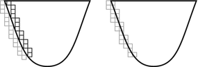

  

  Mesh of the kettledrum. (Left) Separated meshes yielding numerical diffraction. (Right) Fictitious domains method

However, this solution must be rejected because it generates spurious diffraction effects due to the discontinuous (“staircase”) approximation of the bowl’s shape. In order to overcome this difficulty, it is preferable to use the fictitious domain method [32]. In this method (see below) the acoustic variables are calculated in a unique domain Ω, instead of the two separated domains Ω _i and Ω _e , thanks to the introduction of a new “pressure jump” variable across the boundary of the instrument.

2.6.1 Fictitious Domain Method

The fictitious domain method is based on a variational formulation of the problem. Multiplying Eq. (14.12) by an admissible test function w ^∗, and integrating it over the surface $\varSigma$ of the membrane, we get

$$\displaystyle{ \frac{d^{2}} {dt^{2}}\int _{\varSigma }m_{s}ww^{{\ast}}dS =\int _{\varSigma }\text{div}\left [\tau \nabla \left (w +\eta \frac{d} {dt}\right )\right ]w^{{\ast}}dS -\int _{\varSigma }f(t)gw^{{\ast}}dS -\int _{\varSigma }[p]\vert _{\varSigma }w^{{\ast}}dS. }$$

(14.36)

Since the test function w ^∗ must fulfill the boundary conditions of the problem, this function vanishes on the edge $\partial \varSigma$ of the membrane. It can then be checked that the integration by parts of (14.36) yields

$$\displaystyle\begin{array}{rcl} \frac{d^{2}} {dt^{2}}\int _{\varSigma }m_{s}ww^{{\ast}}dS =\int _{\varSigma }\tau \nabla \left (w +\eta \frac{d} {dt}\right )\nabla w^{{\ast}}dS -\int _{\varSigma }f(t)gw^{{\ast}}dS -\int _{\varSigma }[p]\vert _{\varSigma }w^{{\ast}}dS.& & \\ & &{}\end{array}$$

(14.37)

A similar method is applied to the acoustic equations (14.16), through introduction of the test functions p ^∗ and v ^∗, for both the pressure and velocity, for which the boundary conditions are fulfilled. After integration by parts, we get (see [45]):

$$\displaystyle{ \rho \frac{d} {dt}\int _{\varOmega }\boldsymbol{v}\boldsymbol{v}^{{\ast}}d\mathcal{V}-\int _{\varOmega }p\ \text{div}\boldsymbol{v}^{{\ast}}d\mathcal{V} =\int _{\varGamma }[p]\vert _{\varGamma }\boldsymbol{v}^{{\ast}}.\boldsymbol{n}\ dS }$$

(14.38)

and

$$\displaystyle{ \frac{1} {\rho c^{2}} \frac{d} {dt}\int _{\varOmega }pp^{{\ast}}d\mathcal{V} +\int _{\varOmega }\text{div}v\ p^{{\ast}}d\mathcal{V} = 0\, }$$

(14.39)

where $\varGamma =\varSigma \cup \mathcal{C}$ is the total surface of the kettledrum (membrane + bowl), and Ω is the complete space $\mathbb{R}^{3}$. A new variable $\lambda = [p]\vert _{\varGamma }$ appears in Eq. (14.38). This variable is the pressure jump across the surface of the instrument with normal vector $\boldsymbol{n}$. Thanks to the introduction of this new variable, it is as if the unknown pressures p _i and p _e were replaced by the unique variable p and, similarly, the unknown velocities $\boldsymbol{v}_{i}$ and $\boldsymbol{v}_{e}$ were replaced by the unique velocity field $\boldsymbol{v}$. The formulation of the problem is completed by expressing the boundary conditions on the surface Γ:

$$\displaystyle{ \left \{\begin{array}{cl} \boldsymbol{v}.\boldsymbol{n} = \frac{\partial w} {\partial t} \ \ \ \text{in}\ \ \ \varSigma,\\ \boldsymbol{v}.\boldsymbol{n} = 0\ \ \ \text{in} \ \ \ \mathcal{C}.\end{array} \right. }$$

(14.40)

Through integration on Γ, with the introduction of another test function $\lambda ^{{\ast}}$, we get

$$\displaystyle{ \frac{d} {dt}\int _{\varSigma }w\lambda ^{{\ast}}dS -\int _{\varGamma }\boldsymbol{v}.\boldsymbol{n}\lambda ^{{\ast}}dS = 0. }$$

(14.41)

In summary, the fluid–structure problem corresponding to the acoustics of timpani is entirely defined by the system of four equations (14.37)–(14.39) and (14.41), where the four unknowns are the displacement w of the membrane, the pressure p and the acoustic velocity v in space, and the pressure jump $\lambda$ across the surface of the instrument. The numerical formulation of this problem is presented later in this section.

2.6.2 Absorbing Boundary Conditions

The purpose of ABC is to simulate a free space. In this context, the leading idea consists of inserting artificial absorbing conditions at the border of the computational domain. The basic principles of this method are presented here, for the simple case of an half-space. For a cube, additional conditions on the edges and on the corners are necessary [19]. The posed problem is the following: given the wave equation

$$\displaystyle{ \frac{\partial ^{2}p} {\partial t^{2}} - c^{2}\left (\frac{\partial ^{2}p} {\partial x^{2}} + \frac{\partial ^{2}p} {\partial y^{2}} + \frac{\partial ^{2}p} {\partial z^{2}}\right ) = 0\ \ \ \forall (x,y,z) \in \mathbb{R}^{3}, }$$

(14.42)

the aim is to limit the computation in the half-plane z < 0 by imposing a perfectly (totally, or transparent) absorbing condition in z = 0 (see Fig. 14.19). Denoting $\tilde{P } (k_{x},k_{y},z,\omega )$ the Fourier transform of the pressure (in time and space), the conditions amounts to impose:

$$\displaystyle{ \frac{\partial \tilde{P } } {\partial z} + j \frac{\omega } {c}\sqrt{1 - \frac{c^{2 } (k_{x }^{2 } + k_{y }^{2 })} {\omega ^{2}}} \tilde{P }= 0\ \ \ \text{in}\ \ \ z = 0. }$$

(14.43)

Fig. 14.19

Principle of absorbing boundary conditions (ABC) on an half-space

One drawback of the formulation (14.43) is that it is nonlocal in time and space (x, y). As a consequence, the ABC cannot be expressed in the time domain using partial differential equations. In order to overcome this difficulty, the function $\sqrt{ 1 - u}$ (where $u = c^{2}(k_{x}^{2} + k_{y}^{2})/\omega ^{2} <1$) is expanded onto a series of rational functions:

$$\displaystyle\begin{array}{rcl} \sqrt{ 1 - u} \simeq 1 -\sum _{l=1}^{L}\beta _{ l} \frac{u} {1 -\alpha _{l}u} =\gamma -\sum _{l=1}^{L}\frac{\beta _{l}} {\alpha _{l}} \frac{1} {1 -\alpha _{l}u}\ \ \ \text{with}\ \ \ \gamma = 1 +\sum _{ l=1}^{L}\frac{\beta _{l}} {\alpha _{l}},& & \\ & &{}\end{array}$$

(14.44)

where, for stability reasons, the parameters α _l and β _l must fulfill the conditions

$$\displaystyle{ \alpha _{l}> 0,\ \ \beta _{l} \geq 0,\ \ \sum _{l=1}^{L} \frac{\beta _{l}} {1 -\alpha _{l}} <1. }$$

(14.45)

One possible alternative consists of selecting the Padé coefficients defined by:

$$\displaystyle{ \beta _{l} = \frac{2} {2L + 1}\sin ^{2}\left ( \frac{l\pi } {2L + 1}\right )\ \ \text{and}\ \ \alpha _{l} =\cos ^{2}\left ( \frac{l\pi } {2L + 1}\right ). }$$

(14.46)

Auxiliary variables are the defined:

$$\displaystyle{ \tilde{\varPhi }_{l} = \frac{\omega ^{2}} {\omega ^{2} -\alpha _{l}c^{2}(k_{x}^{2} + k_{y}^{2})} \tilde{P } . }$$

(14.47)

The ABC can then be rewritten on the form of the following system:

$$\displaystyle{ \left \{\begin{array}{cl} &\frac{d\tilde{P } } {dz} + j \frac{\omega } {c}\left (\gamma \tilde{P }-\sum _{l=1}^{L}\frac{\beta _{l}} {\alpha _{l}} \tilde{\varPhi } _{l}\right ) = 0 \\ &\left [\omega ^{2} -\alpha _{l}c^{2}(k_{x}^{2} + k_{y}^{2})\right ]\tilde{\varPhi }_{l} =\omega ^{2}\tilde{P } .\end{array} \right. }$$

(14.48)

Finally, returning back to the time domain through inverse Fourier transform, we get

$$\displaystyle{ \left \{\begin{array}{cl} &c\frac{\partial p} {\partial z} +\gamma \frac{\partial p} {\partial t} -\sum _{l=1}^{L}\frac{\beta _{l}} {\alpha _{l}} \frac{\partial \phi _{l}} {\partial t} = 0, \\ &\frac{\partial ^{2}\phi _{ l}} {\partial t^{2}} -\alpha _{l}c^{2}\left ( \frac{\partial ^{2}\phi _{ l}} {\partial x^{2}} + \frac{\partial ^{2}\phi _{ l}} {\partial y^{2}} \right ) = \left.\frac{\partial ^{2}p} {\partial t^{2}} \right \vert _{z=0}\ \ \ \ \text{for}\ \ l = 1,\ldots,L. \end{array} \right. }$$

(14.49)

In practice, approaching the condition of perfect transparency (i.e., no wave returning from z = 0) as close as possible depends on the order L of the expansion (the higher the number of auxiliary variables ϕ _l , the better the approximation). The system (14.49) can be seen as a transport equation along z coupled to L 2-D wave equations in the plane z = 0.

2.6.3 Numerical Discretization

The numerical resolution of the timpani model consists of seeking for discrete approximations ($p_{h},\mathbf{v_{h}},w_{h},\lambda _{h},\xi _{h}$) for the variables of the problem: the pressure p, the acoustic velocity v, the displacement of the membrane w, the pressure jump $\lambda$, and the mallet’s displacement $\xi$. The index h indicates that we are dealing here with a spatial discretization obtained from the meshes of the constituting elements of the the kettledrum coupled to the free space. For these approximations, the finite element method is used (see Chap. 1).

Figure 14.20 shows the meshes used by Rhaouti [44]. The space Ω is discretized with a cubic mesh. The pressure p _h and the velocity v _h are associated with each elementary cube. For the pressure jump $\lambda _{h}$, P1 finite elements are used. These elements can be viewed as a 2-D generalization of the hat functions presented in Chap. 1. A triangular mesh is selected on the surface of the instrument. Finally, a triangular mesh and P1 finite elements also are used for the displacement w _h of the membrane. Since the speed of the flexural waves is usually three to four times smaller than the speed of sound, the elastic wavelength also is three to four times smaller than the acoustic wavelength, for a given frequency. In order to ensure the coherence between all numerical schemes, a similar ratio between wavelength and mesh size must be selected for the variables. For this reason, the size of the mesh elements on the surface for w _h is selected here so that the spatial step is four times smaller than for the pressure jump $\lambda _{h}$.

Fig. 14.20

Mesh of the different constitutive elements of the kettledrum. (a) Cubic mesh for the pressure p _h and the acoustic velocity v _h. (b) Finite elements P1 for the pressure jump $\lambda _{h}$. (c) Refine previous P1 mesh for the displacement w _h on the membrane

After the space discretization, the equations of the problem are reduce to a matrix system of time differential equations, similar to the example shown in Chap. 1. We have

$$\displaystyle{ \left \{\begin{array}{cl} &f_{h} = K\left [(\delta -\xi _{h} + \mathbf{G^{t}}w_{h})^{+}\right ]^{\alpha }, \\ &m\frac{d^{2}\xi _{ h}} {dt^{2}} = f_{h}, \\ &\mathbb{M}_{w}\frac{d^{2}w_{ h}} {dt^{2}} + \mathbb{R}_{w}w_{h} +\eta \mathbb{R}_{w}\frac{dw_{h}} {dt} + \mathbb{A}_{w}\lambda _{h} = -\mathbf{G}f_{h}, \\ &\mathbb{M}_{p}\frac{dp_{h}} {dt} + \mathbb{D}_{v}^{t}\mathbf{v_{h}} = 0, \\ &\mathbb{M}_{v}\frac{d\mathbf{v_{h}}} {dt} - \mathbb{D}_{v}p_{h} - \mathbb{B}_{v}\lambda _{h} = 0, \\ &\mathbb{B}_{v}^{t}\mathbf{v_{h}} - \mathbb{A}_{w}^{t}\frac{dw_{h}} {dt} = 0, \end{array} \right. }$$

(14.50)

where $\mathbb{M}_{w}$, $\mathbb{R}_{w}$, $\mathbb{M}_{v}$, $\mathbb{D}_{v}$, $\mathbb{B}_{v}^{t}$, and $\mathbb{A}_{w}^{t}$ are matrices, and where G is a vector accounting for the spatial extent of the mallet’s impact on the membrane. This system can be discretized in time using finite differences , as seen in Chap. 1.

3 Example of the Guitar

3.1 Introduction

Various aspects of the acoustics of guitars have been addressed a number of times in the previous chapters of this book. The vibrations of plucked strings, for example, were presented in detail in Chap. 3. In Chap. 5, the dissipation mechanisms encountered in the different constitutive parts of the instruments were analyzed. The coupling between string and soundboard , and the soundboard-cavity coupling were studied in Chap. 6 Finally, the general results on the radiation of plates, and the plate-air interaction studied in Chap. 13 are also applicable to the guitar. These previous investigations are pursued here where the interaction between air and soundboard is now extended to the whole spectrum of the instrument (up to 5 kHz) and not only limited to the low-frequency range as in Chap. 6 ¹² Another new feature of the model presented here is that the complex interactions between cavity, soundboard, and the external air are taken into account. This additional feature is made possible through application of the fictitious domain method (presented in the previous section devoted to the timpani), which allows to consider the fluid domain (internal cavity and external space of the guitar) as a whole.

The classical guitar (in contrast to the electric guitars without an air cavity) has the particularity to show a sound hole in the soundboard . As a consequence, the air cavity is not closed, and the acoustic field has no discontinuity between inside and outside. An appropriate model should account for this specificity. The average diameter of the sound hole is 10 cm, which corresponds to an half acoustic wavelength at a frequency of 1.7 kHz. In comparison, the spectrum of guitar sounds usually shows significant energy up to 5 kHz. Thus, it is not possible to ignore the presence of this hole, in contrast with the previous case of timpani where the diameter of the hole was significantly smaller than the smallest acoustic wavelength of timpani sounds.

As for timpani, we have to consider the interaction between the vibrating parts of the guitar and the acoustic field. The soundboard is the main radiating part of the instrument, though, in some circumstances, the back plate also might contribute to the total sound. The radiation of the other parts will be ignored in this section. Compared to a membrane, the guitar soundboard is heavier and stiffer. However, as discussed later, the acoustic pressure can affect its vibratory behavior. It should be noticed that the pressure inside the cavity can be very high.¹³

In what follows, a recent guitar model is presented [22]. This presentation is complemented by considerations on the acoustic intensity radiated by the instrument [1]. Finally, a summary of power balance between all the constitutive parts of the instrument is conducted. In this section, the equations of the model that present similarities with the timpani model are not detailed. We content ourselves with the presentation of the specificity of the guitar model, and we rather focus on the significant physical results of the instrument (admittance, intensity, sound power, damping factors, and decay times) that the model is able to account for. The relevance of fluid–structure interaction in the case of the guitar is particularly emphasized. Most of these results can be generalized to other stringed instruments.

3.2 Physical Model

In the guitar model presented below, several elements are coupled together:

• The string(s). The flexural motion of the string is assumed to be perpendicular to the soundboard plane (one polarization). The internal damping is represented by the association of a viscous (“fluid”) damping term and a viscoelastic term (see Chap. 5). The excitation of the string by the finger is represented by a idealized impulse localized in time h(t) and space g(x), see Fig. 14.21. The impulse h(t) is made of the association of two cosine functions accounting for a slow increase followed by a fast decrease, and is inspired by experimental results (see [11]). Is also accounts, to a first approximation, for stick-slip mechanisms between the finger and the string (see Chap. 1). The function g(x) is here a Gaussian function (though other smooth functions could be used) and accounts for the finite width of the finger on the string [23].

  Fig. 14.21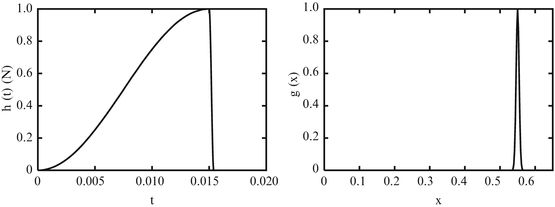

  

  Idealized force impulse on the string. (Left) Time dependence h(t). (Right) Spatial extent g(x)

  Fig. 14.22

  

  Mesh used for the string, the soundboard and the pressure jump

• The soundboard . An orthotropic plate model is used for the soundboard (see Chap. 1). The shape of the plate is that of a standard guitar. The presence of the bridge and of the ribs is represented by spatial heterogeneities of both the density ρ _p (x, y) and thickness h(x, y). The amount of internal damping depends on the material, and is derived from experiments. The soundboard is assumed to be clamped at its periphery, and free on the edge of the sound hole. Considering the small mean value of the thickness, it is further assumed that the Kirchhoff–Love model is applicable. The soundboard is excited by the force transmitted by the string to the bridge, and by the pressure force on its both sides. The other parts of the instrument are supposed to be perfectly rigid.

• The acoustic field. Here, the model is close to the one presented in Sect. 14.2 for timpani [see Eq. (14.16)]. A condition of continuity for the velocity normal to the soundboard is added, as well as a null condition for the normal velocity on the other constitutive parts of the instrument.

Limitations of the Present Model

The present coupled model shows an additional degree of complexity, compared to other elementary models where each constitutive part (soundboard, cavity, …) is treated separately. In this chapter, attention is put on radiation, and thus we focus on the soundboard-acoustic field coupling. However, with the objective to model a real instrument more accurately, then several refinements should be added. Without pretending to be exhaustive, several possible additional features are the following:

• (1) As indicated in the previous Chaps. 6 and 8, the motion of the string is complex and cannot be reduced to a single polarization perpendicular to the soundboard. Several factors also induce a parallel component: the motion of the bridge, the slipping of the string along the fret, and nonlinearities due to large amplitude motion.

• (2) The modal analysis of a guitar shows that one of the lowest modes corresponds to a flexural mode of the neck (free at one end, and loaded by the body at the other end). The corresponding eigenfrequency is of the order of magnitude of a few Hz. As a consequence, this mode does not directly contribute to the audible radiated acoustic pressure. However, the flexion of the neck induces fluctuations of length (and, in turn, fluctuations of tension) in the attached strings. In conclusion, the coupling between the neck and the strings should be taken into account in a future model.

3.3 Specificity of the Numerical Guitar Model

3.3.1 Spatial Discretization

A six strings guitar model that couples the soundboard with the air has been solved numerically with a method similar to the one used for timpani [3]. Both models are briefly compared and summarized below.

• The main difference between both instruments is due to the presence of a plate operator for the guitar soundboard, compared to a 2-D wave equation in the case of timpani membrane. This operator contains fourth-order space derivatives (see Chaps. 1, 3 and 13). In order to use standard finite elements , the fourth-order equations are replaced by second-order systems of equations where the new variables are the velocity and the flexural moment.

• As for the kettledrum, the fluid–structure interaction problem is solved with the fictitious domain method . For the guitar, this method has two main advantages: it allows to avoid distinct pressures meshes inside and outside the cavity and, in addition, it facilitates the treatment of the pressure continuity through the sound hole. In this context, the present method is more efficient than those where the cavity is considered separately (see, for example, [46]), or those requiring an artificial ectoplasm (a massless vibrating element) at the sound hole [6].

• The string equation is replaced here by a system of first-order partial differential equations, where both unknowns (force and velocity) are discretized with finite elements.

• The acoustic field (inside and outside the cavity) is discretized with the same scheme as for the kettledrum.

3.3.2 Time-Domain Discretization

The time-domain discretization of both the string and acoustic equations is achieved with second-order centered finite difference schemes , as for the kettledrum. The main difficulty arises from the soundboard equation .

The stability condition for the plate, with explicit second-order finite differences , is of the form Δ t ≤ A∕h _p ², where A is a parameter depending on the material used for the plate, and h _p is the spatial step. This means, for example, that the sampling frequency must be multiplied by 4, if the spatial mesh is refined by a factor 2. Such a condition rapidly becomes very cumbersome as soon as the objective is to extend the spectral domain of the sound to be simulated. By comparison, we have the condition $\varDelta t_{\max } \propto 1/h$ for the wave (or the string) equation, which is less demanding.

In order to overcome this difficulty, one can use a pseudo-spectral method [22]. The method consists, first, in calculating the in vacuo modes of the soundboard, using spatial finite elements. This yields a system of decoupled differential equations where the damping terms can be added separately for each mode. For each damped oscillator equation, the source term is the projection of the forces exerted by the string and the pressure on the soundboard. These source terms are updated at each time step. Notice that the time step for the soundboard must be compatible with the time steps selected for the other constitutive parts of the instrument (string and air).

In practice, computing the first 50 modes of the soundboard yields a satisfactory simulation of the sound field up to 3 kHz. The average distance between consecutive modes is then Δ f = 60 Hz. As an illustration, Eq. (13.142) in Chap. 13 yields Δ f = 57 Hz with the following data: $\rho _{p} = 350\,\text{kg/m}^{3}$, E ₁ = 15. 10⁹ Pa, $E_{2} = E_{1}/17$, ν = 0. 3, h = 2. 9 mm, S = 0. 1 m².

3.4 Admittance at the Bridge

The admittance at the bridge is a key variable influencing the coupling between the “engine” of the instrument (the strings) and the resonator (the soundboard coupled to both the air cavity and external air). Therefore, computing this quantity is an appropriate means of quantifying the effects of coupling. The following results were obtained by using Derveaux’s model described in Sect. 14.3.2. The values of the geometrical and material parameters are extracted from the literature (see, for example, [28, 29]). One advantage of the model is to compare the behavior of the guitar successively in vacuo and in air.

Figure 14.23 shows the simulated admittances at the bridge for a guitar with a soundboard of thickness 2.9 mm, and a cavity of height 10.4 cm. The two first figures show a comparison between the simulated admittances between 0 and 800 Hz, at the point of the bridge corresponding to the position of the lowest E-string (with fundamental 83 Hz), in vacuo and in air, respectively. One can see that the influence of both external air and cavity is reflected in a shift of the spectral peaks, and by the emergence of additional peaks.

Fig. 14.23

Admittance at the bridge of a guitar at the attachment point of the 6th E-string (83 Hz). (a) In vacuo soundboard. (b) Soundboard coupled to air and cavity: [0–800] Hz. (c) Soundboard coupled to air and cavity: [0–3000] Hz. Simulation based on the model by Derveaux et al. [23]

Below 250 Hz, the admittance curve in air shows the same shape as for the simplified low-frequency two-oscillators model presented in Chap. 6 [17]. The third figure shows the simulated admittance up to 3 kHz. Its general shape is similar to those observed experimentally (see, for example, [8] or [49]). With the selected parameters, the mean value of the admittance between 0 and 1 kHz is approximately 10 dB above its mean value between 1 and 2.5 kHz, which shows a higher mobility in the low-frequency domain. The peaks are clearly separated for f < 1 kHz, whereas they overlap more and more with increasing frequency. This overlapping can be attributed to both the air-structure coupling and damping phenomena (material damping and radiation). The imbalance between low and high frequency domains is reinforced if the thickness of the soundboard decreases. With an average thickness divided by a factor of 2 (1.45 mm), the mean value of the admittance between 0 and 500 Hz is roughly 15 dB below its mean value between 500 and 2500 Hz [23].

3.5 Damping Factors

The admittance curves are complemented by the damping factors shown in Fig. 14.24. These factors are the imaginary parts of the eigenfrequencies which govern their decay times. The damping factors α of the in vacuo soundboard (asterisk symbol), and of the soundboard coupled to air and cavity (inverted triangle symbol), are represented on the left figure. These values are derived from time-frequency analysis of the impulse responses of the bridge velocity, at the attachment point of the 6th E-string (83 Hz). Not surprisingly, the curve α(f) for the in vacuo soundboard is in accordance with the linear law selected for the structural damping in the model. For the soundboard coupled to external air and cavity, the mean value of the damping factors is higher than in the previous case. However, the variations from one mode to the next is more erratic. Due to multiple coupling between soundboard and air modes, some of the modes even show a smaller global damping factor than the structural damping factor (at the same frequency), whereas the neighboring frequencies are more damped. It is as if some of the modes receive energy from their neighboring modes through air-structure coupling.

Fig. 14.24

Damping factors α (in s⁻¹). (Left) Comparison between the damping factors of the in vacuo soundboard modes (asterisk symbol), and of the soundboard coupled to external air and cavity (inverted triangle symbol). (Right) Comparison between the damping factors of the isolated open E2 string modes (asterisk symbol), the string modes coupled to the in vacuo soundboard (square symbol), and the string modes coupled to the complete guitar (inverted triangle symbol). Simulations based on the model by Derveaux et al. [23]

Similar conclusions can be drawn for the strings. Figure 14.24 (right) shows a comparison between the damping factors α of a isolated open E2 string (asterisk symbol), with fundamental 83 Hz, and of the same string coupled to the in vacuo soundboard (square symbol) and to a complete guitar (inverted triangle symbol), successively. The curve α(f) is a parabola, which is coherent with the selected damping model made of the association of a fluid damping term and a viscoelastic damping term. Due to the coupling of the string with the in vacuo soundboard , the damping factors globally increase. However, the increase in damping fluctuates from one mode to the next, depending on the degree of proximity between soundboard and string modes (see Chap. 6). Finally, the coupling of the soundboard with air and cavity yields an additional increase of the average damping, though with significant variations from one mode to the next. Such fluctuations are currently observed on real guitars [50].

3.6 Radiated Sound Field

Figure 14.25 shows five successive snapshots of the pressure field radiated by a simulated guitar in its symmetry plane, right after the initial plucking of the 1st open string (E4: fundamental 330 Hz). The delay between consecutive snapshots is 0.36 ms. At first (snapshots 1 and 2), the pressure field is omnidirectional and is mainly due to the vibration of the soundboard. In the meantime, the magnitude of the pressure field inside the cavity increases progressively. From snapshot 3, the cavity radiates through the sound hole. The internal field is partially in phase with the motion of the soundboard, and partially in antiphase. On snapshots 4 and 5, the cavity field progressively becomes in total antiphase with the external field. As a result, a decrease of pressure followed by an inversion of the outside pressure is observed. The instantaneous directivity of the pressure field is complex and evolves rapidly with time. This is a consequence of the large number of excited modes (between 0 and 3 kHz), where each mode has its own directivity pattern and its own temporal evolution. As observed in timpani, the global directivity of the instrument stabilizes after a certain amount of time (typically within one second). At this time, the sound of the guitar is governed by a relatively low number of string’s partials.

Fig. 14.25

Successive snapshots of the pressure field radiated by the guitar, right after an initial pluck of the 1st open string (E4: fundamental 330 Hz). Simulations based on the model by Derveaux et al. [22]

3.7 Acoustic Intensity and Power Balance

3.7.1 Acoustic Intensity

In the model used in the section for illustrating the acoustics of guitars through simulations, we take benefit from having at our disposal both the pressure and the acoustic velocity field to compute the acoustic intensity $\mathbf{I} = p\boldsymbol{v}$. Figure 14.26 shows an example of the useful information provided by this variable. In this Figure, the intensity I is shown in three perpendicular planes, successively: the symmetry plane of the instrument, one horizontal plane close to the soundboard , and one vertical plane perpendicular to the neck and passing through the box. The acoustic intensity is here averaged over one period, for a forced sinusoidal excitation close to one mode of the complete guitar (272 Hz). As shown in Chap. 1, the acoustic intensity is linked to the energy density through its divergence. As a consequence, the intensity vectors are oriented towards the regions of space with increasing acoustic energy. A “source” is characterized by a set of diverging vectors, whereas a “sink” is a region where the intensity vectors converge. In Fig. 14.26, one can see both the internal and external sources and the regions of space (above the soundboard, in particular) where the energy density vanishes, due to opposition of phase between sources.

Fig. 14.26

Acoustic intensity for the guitar mode at 272 Hz. (Left) Plane perpendicular to the neck. (Middle) Symmetry plane of the guitar. (Right) Horizontal plane, 1 cm above the soundboard. After [1]

Fig. 14.27

General configuration of the piano model

3.7.2 Radiated Power and Acoustical Efficiency

At this point, we are now able to compute the acoustical efficiency of the guitar (see also Chaps. 2 and 13), defined as:

$$\displaystyle{ \zeta = \frac{\langle \mathcal{P}_{a}\rangle } {\langle \mathcal{P}_{i}\rangle }, }$$

(14.51)

where $\mathcal{P}_{a}$ is the mean value of the radiated power, and $\mathcal{P}_{i}$ is the mean value of the total power dissipated in the instrument. For simplicity, only one string is considered. We have

$$\displaystyle{ \langle \mathcal{P}_{i}\rangle =\langle \mathcal{P}_{a}\rangle +\langle \mathcal{P}_{c}\rangle +\langle \mathcal{P}_{s}\rangle }$$

(14.52)

where $\langle \mathcal{P}_{c}\rangle$ is the mean power dissipated in the string, and $\langle \mathcal{P}_{s}\rangle$ is the mean power dissipated in the body.

Let us now consider one particular frequency component ω _n of the string’s spectrum for which the mean power dissipated over one period $T_{n} = 2\pi /\omega _{n}$ is calculated. We denote V _n the modal amplitude of the string’s velocity, and r _n the modal resistance corresponding to the internal losses. The quality factor is then given by $Q_{n} =\omega _{n}m_{n}/r_{n}$, where m _n is the modal mass [33]. The mean power dissipated in the string for this partial is written

$$\displaystyle{ \langle \mathcal{P}_{c}\rangle (\omega _{n}) = \frac{1} {2}r_{n}V _{n}^{2}. }$$

(14.53)

When the string is coupled to the soundboard (at position x = L), it was shown in Chap. 6 that the mean power dissipated at the end (or, equivalently, the power transferred from string to soundboard) is written

$$\displaystyle{ \langle \mathcal{P}_{L}\rangle (\omega _{n}) = \frac{1} {2}Z_{c}^{2}\mathfrak{R}e\left \{Y (\omega _{ n})\right \}V _{n}^{2}. }$$

(14.54)

In (14.54), Y is the driving point admittance of the bridge at the attachment point, for the soundboard loaded by the air. $\langle \mathcal{P}_{L}\rangle$ accounts for all acoustic and structural losses in the loaded body at frequency ω _n : $\langle \mathcal{P}_{L}\rangle =\langle \mathcal{P}_{a}\rangle +\langle \mathcal{P}_{s}\rangle$. In summary, the mean power dissipated in the guitar at frequency ω _n is written

$$\displaystyle{ \langle \mathcal{P}_{i}\rangle (\omega _{n}) =\langle \mathcal{P}_{c}\rangle (\omega _{n}) +\langle \mathcal{P}_{L}\rangle (\omega _{n}). }$$

(14.55)

Experimentally, r _n can be derived from measurements performed on an isolated string, or, alternatively, on a guitar where the soundboard is blocked. The quantity Y (ω) can be obtained from standard admittance measurements (see Chap. 3). Using finally Eqs. (14.53) and (14.54), one can calculate the efficiency for a given ω _n .

Table 14.2 shows the values obtained for the acoustical efficiency, at some particular frequencies, using the guitar model by Derveaux et al. These values are coherent with measurements performed on real guitars by Boullosa et al. These authors have shown, among other things, that a link exists between the acoustical efficiency of the guitar and the subjective evaluation of its quality for both the players and listeners. From the point of view of the player, the input mechanical energy that can be transmitted to the guitar is limited in terms of maximum force and string displacement. Thus, it is essential that a significant part of this energy can be converted into sound power without excessive effort that would deteriorate the sound quality. A noticeable efficiency is necessary so that the guitarist can have enough dynamic range at its disposal in order to introduce subtleties in the played music. However, one must keep in mind that other quality factors of the instrument are essential for playing “good” music, such as the spectral balance between bass and treble sounds, and the clarity of the attack. Last but not least, the talent of the player cannot be ignored!

Table 14.2 Acoustical efficiency of the guitar

In conclusion, a guitar tone is a free oscillation: the total dissipated power is the sum of the power dissipated by both the strings and the air-loaded body. The power dissipated by the soundboard modes takes place during the initial part of the sound, since their quality factors are significantly smaller than those of the strings (see Chap. 6). After this transient part, the main part of the radiated power is concentrated in the partials of the strings. Audibly, a guitar tone is schematically made of a short “body” sound followed by a long “string” tone.

In this section, attention was mostly paid on classical guitars with nylon strings. Electric guitars are characterized, in particular, by a more massive body and the use of steel strings, which induce a significantly different tone quality. For more information on electric and steel strings guitars, one can refer to [38, 40–42].

4 Example of the Piano

4.1 General Presentation of the Model

A piano sound is the result of free oscillations, as for guitars and timpani in their normal use. As the player presses a key, a complex mechanism is activated whose main effect is to project the hammer against the strings with an impact velocity that depends on the depression conditions of the key [48]. In what follows, the key mechanism is ignored. The consecutive vibrations of the hammer shank also are ignored. A recent study by Chabassier and Duruflé highlights the relevance of these vibrations [10].

The model starts as the very instant where the hammer hits the strings, taken as the origin of time. The purpose is to model the succession of vibratory and acoustic phenomena in hammer, strings, soundboard, and surrounding air.

The strings are set into motion by the blow of the hammer. Their motion is a combination of transverse and longitudinal waves. These waves are nonlinearly coupled, due to the variation of the tension with amplitude, as shown in Chap. 8. These nonlinear phenomena greatly influence the properties of piano sounds: they are responsible for the presence of pitch glide and phantom partials. In this section, the nonlinear equations of strings presented in Eq. (8.62) will be used. Another nonlinear feature exists in the hammer–string interaction, due to the compression of the felt, as seen in Chap. 1. The interaction force is modeled here as a power law, as for the interaction between a mallet and a timpani head. The main consequence of this nonlinearity is to widen the excited spectral domain (due to shortening of the force impulse) as the hammer impact velocity increases.

An orthotropic Reissner–Mindlin (or thick plate) model is selected for the piano soundboard [9]. Such a model can be viewed as equivalent to the Timoshenko model for plates, in the sense that it accounts for the shear stresses, so that the transverse displacement is coupled to the rotation of the cross-sections [43]. Such a model, which is more complex than the Kirchhoff–Love model used for the guitar , is firstly justified by the spectral extent of most piano sounds (up to 15 kHz and even more) and, secondly, because of the presence of bridge and ribs. Due to these elements, the assumption of thin plate is no longer valid. The ribs and the bridge are taken into account as heterogeneities in thickness and material properties of the soundboard, as for the guitar model presented in the previous section. Figure 14.28 illustrates this method in the case of a grand piano (Steinway D).

Fig. 14.28

Grand piano soundboard model. The thin grey stripes indicate the direction of the fibers. The ribs (in dark grey) and the bridge (in black) are treated as heterogeneities

The coupling between the soundboard and a string has to be expressed by dual conditions, in order to conserve the energy: one condition for the force and another for the velocity. The force exerted by the string is given in Eq. (8.64) in Chap. 8. Assuming that the motion of the bridge is purely vertical (an assumption that could eventually be revised), then one has to write a condition of continuity for the vertical components of both string and bridge velocities, and a condition of nullity for the horizontal motion of the bridge.

The conditions of coupling between the structure of the piano and the acoustic field can be written with a similar method as for the guitar and the kettledrum. The linear acoustic equations in the surrounding air are the same as in Eq. (14.16). It is supposed here that only the soundboard vibrates, all other parts of the instrument remaining rigid. Thus, a continuity of the normal velocity is written on the soundboard, and a condition of nullity of the normal acoustic velocity is written on the other parts. We are aware of the fact that this is an approximation since, in reality, one can clearly feel with the fingers that the rim of a grand piano vibrates, especially when playing notes in the bass range.

The free space is simulated here using perfectly matched layers (PML). The method consists of simulating a fictitious layer of absorbing material along the boundaries of the computational domain, in order to limit as much as possible the reflected waves [2].

An equation of energy conservation can be written for the complete model composed by the hammer, the strings, the soundboard, and the acoustic field, as illustrated in Fig. 14.29. This energy conservation is then used for deriving numerical schemes with the guarantee of stability.

Fig. 14.29

Temporal evolution of the energy for note C2 (fundamental f = 65. 4 Hz). Thin solid line: total energy; dashed line: hammer energy; dash-dotted line: string energy; dotted line: soundboard energy; thick solid line: air (acoustic) energy. (Left) Linear scale; (Right) logarithmic scale

4.2 Modal Analysis of the Soundboard

The dynamics of the soundboard is governed by a plate operator. As for the guitar [23], it is preferable to solve this part of the model in two steps because of the required accuracy in the calculation of the frequencies (numerical dispersion). In a first step, a modal analysis is conducted on the undamped soundboard (i.e., the terms of losses are not considered in the equations). The soundboard equations are discretized in space, using high-order finite elements . For a grand piano, typically 2400 modes are necessary for predicting accurately the vibrations of the soundboard between 0 and 10 kHz.

Figure 14.30 shows a few calculated modes for a Steinway D soundboard, with fourth-order finite elements and 450,000 degrees of freedom. Examining the shapes of the higher modes confirms the results presented in Chap. 3 for an upright piano: here also, the vibrational energy is localized in relatively narrow areas, frequently bounded by the ribs and/or the bridge.

Fig. 14.30

Examples of some simulated modes of a grand piano soundboard (Steinway D)

In a second step, once the soundboard modes are obtained, each modal amplitude X _n (t) associated to the modal frequency f _n is governed by a second-order differential equation, as shown several times in Chap. 3. Then, a convenient way to account for the observed damping in the soundboard material (wood) is to introduce in these oscillator equations a damping term whose value is derived either from experiments or from available data in the literature for the appropriate species. We get

$$\displaystyle{ \frac{d^{2}X_{n}} {dt^{2}} +\alpha (f_{n})\frac{dX_{n}} {dt} + \left (2\pi f_{n}\right )^{2}X_{ n} = F_{n}, }$$

(14.56)

where the terms F _n are the modal projections of the source terms. These terms are composed by both the string forces and acoustic pressure due to the radiated field. Recall that introducing a posteriori damping terms in the decoupled equations (14.56) is justified as long as the damping factors are reasonably small compared to the eigenfrequencies (see Chap. 5). Usually, this assumption of diagonal damping is justified for the wood species of current use for making the soundboard, for which the damping coefficients are of the order of a few percents [27].

The damped oscillator equations (14.56) yield analytical solutions which can be discretized with any time step, without altering the dispersion, and with no risk of instability. The appropriate selected time step must be synchronized with those used for the other constitutive parts of the piano (strings and acoustic space).

Recent studies on the vibroacoustics of the piano soundboard were made by Boutillon and Ege [7]. Mamou-Mani et al. investigated the influence of prestress on the eigenfrequencies of piano soundboards [37].

4.3 Results of the Simulations

Figure 14.31 shows the temporal evolution of some simulated variables for the note C2 (fundamental f = 65. 4 Hz) during the first milliseconds of the sound, using the piano model presented above [9].

Fig. 14.31

Temporal evolution of some simulated variables for the note C2 (fundamental f = 65. 4 Hz) using a grand piano model (Steinway D). The transverse displacement of the string is shown on the top of the figures, the longitudinal displacement is drawn in gray color in the line thickness. The displacement field of the soundboard is shown in the bottom of the figures, and the pressure field is shown in two planes perpendicular to the soundboard. The snapshots are calculated at the successive instants of time: (a) 0.4 ms; (b) 1.1 ms; (c) 2.1 ms; (d) 3.1 ms; (e) 4.1 ms; (f) 5.1 ms; (g) 7.1 ms; (h) 8.1 ms; (i) 16.1 ms

The transverse displacement of the string is shown on the top of the figures, the longitudinal displacement is drawn in gray color in the line thickness. It can be seen that the longitudinal perturbation reaches the end (bridge side) well before the transverse wave, in accordance with the ratio between the speed of these waves (around 14). The displacement field of the soundboard is shown in the bottom of the figures, and the pressure field is shown in two planes perpendicular to the soundboard . These planes cross at the attachment point of the string (C2) on the bridge. It can be seen that the soundboard starts to vibrate in picture (b), approximately one millisecond after the impact of the hammer: this initial vibration is due to the longitudinal wave, since the transverse wave has not reached the bridge at that time. From Fig. 14.31b–f, the longitudinal wave excites the soundboard modes, which yield a significant contribution to the attack of piano tones. On the waveforms, this contribution takes the form of the so-called precursor whose magnitude increases with the loudness of the tone, which is in accordance with the nonlinear model of the string [15]. This property is illustrated in Fig. 14.32, for the note D$\sharp 1$.

Fig. 14.32

(Left) Measurements and (Right) simulations of the acoustic pressure radiated by a grand piano (Steinway D) for different levels of excitation: (top) forte; (middle) mezzoforte; (bottom) piano. Note D$\sharp$ 1 (fundamental f = 39 Hz)

Figure 14.33 shows the spectral analysis of measured and simulated piano tones for the note D$\sharp$ 1 played on a Steinway D, for different levels of attack.

Fig. 14.33

Spectra of the sound pressure radiated by a Steinway D grand piano for different levels of excitation: (top) forte; (middle) mezzoforte; (bottom) piano. Note D$\sharp$ 1 (fundamental f = 39 Hz). Left: measurements; Right: simulations

It can be seen first that the domain of excited frequencies increases towards the high frequencies as the initial velocity of the hammer increases. This is a consequence of the decrease of the impulse duration due to stiffening of the hammer’s felt. In each spectrum, the presence of a dense packet of frequencies between 0 and 800 Hz superimposed to the string’s partials is also observed. This packet, which remains almost unchanged from one spectrum to another, is made of the lowest modes of the soundboard. These modes are excited by the strings: the lowest soundboard modes are less damped than those in the medium and high range, and this is the reason why they are more visible on the spectra. Although all soundboard modes are significantly more damped than the strings’ modes, they are clearly audible during the attack transients. Cutting artificially the first milliseconds of a piano tone, then a rather poor “string” tone is obtained. Finally, Fig. 14.33 shows that the spectra are enriched in some specific frequency bands, as the amplitude increases. In the present case, such an enrichment is visible around 1.2, 1.7, 2.3, 2.8, 3.3, 3.7, and 3.9 kHz. As shown in Chap. 8, these additional peaks are phantom partials, due to nonlinear combination of both the transverse and longitudinal waves on the string.

4.4 Radiation and Directivity of the Piano

In this section, the purpose is to investigate the influence of ribs and bridge on the radiation of the piano, with special emphasis on the directivity of the instrument in the medium and high frequency range. This study is related to the localization of modes presented in Chap. 3 [16].

The problem is illustrated here by simulations of directivity performed on a model of upright piano soundboard with equally spaced ribs, without the bridge. Figure 14.34 shows the directivity of the pressure field in two (almost perpendicular) particular planes in the direction of the ribs, and in the direction of the fibers, respectively. At frequency f = 2078 Hz, the inter-ribs distance corresponds here exactly to the half of a vibratory wavelength. The sound field is calculated on a hemisphere with radius r = 3 m. Both directivity patterns show a number of narrow peaks, which means that the radiated energy is concentrated in narrow solid angles. This is nothing but a particular case of antenna effect, comparable to those seen in the previous chapters for plates and wind instruments: in all these situations, the directivity is reinforced for equally spaced arrays of identical sources.

Fig. 14.34

(Top) Calculated displacement field for an upright piano soundboard with equally spaced ribs, at frequency f = 2078 Hz. (Middle) Directivity D($\theta$) in the direction of the ribs (X axis). (Bottom) Directivity D(ψ) in the direction of the fibers (Y axis)

By contrast, Fig. 14.35 shows the directivity patterns obtained from a measured velocity field on an upright piano soundboard, at a forcing frequency f = 1542 Hz. The real soundboard here has a slightly irregular distribution of ribs and two bridges. As a consequence, localized modes, and also localized operating deflexion shapes (ODS) are observed. Recall that ODS are combination of modes with close eigenfrequencies, that are currently observed for forced excitation (see Chap. 3). Due to damping, the modes of a real structure generally cannot be separated beyond a certain frequency (usually beyond 1–1.2 kHz for piano soundboards), and ODS are measured. In a recent paper, it was shown that the localization of modes also can lead to localization of ODS, which corresponds to experiments [16]. As a result of this localization, the array equivalent to the soundboard is made of a significantly small number of sources, compared to the case presented in Fig. 14.34. Thus, the directivity patterns show only one main lobe (along ψ) and two main lobes (along $\theta$). In addition, these calculated patterns are very well predicted by those resulting from an equivalent array of 4 × 2 monopoles (see Fig. 14.35). In conclusion, one practical result of mode localization in the piano, which occurs primarily in the medium and high frequency range, is that the opening of the main lobe is wider as with a regularly spaced ribs pattern. In consequence, the spectral distribution of the radiated sound is not subjected to strong variations, as the direction of observation changes around the instrument, which is rather a favorable property. At this stage, one remaining question is to know whether this interesting effect is really wanted (and controlled) by the piano makers.

Fig. 14.35

(a) Measured velocity field on an upright piano at f = 1542 Hz. (b) Array of 4 × 2 monopoles presenting the same geometrical properties as the vibratory zones of the soundboard. (c) Directivity pattern D($\theta$) along the X-axis (direction of the ribs) and (d) along the Y-axis (direction of the fibers): these patterns were calculated from the measured velocity field (solid line) and from the array of monopoles (dashed line), respectively

5 Radiation of Wind Instruments with Several Orifices

In Chap. 12, we explained that at low frequencies the orifices of wind instruments radiate as monopoles , because their dimensions are small compared to the wavelength. This is true, in particular, for woodwinds, even for saxophones which belong to this category, although these instruments have rather wide orifices. The present section aims to show how multiple sources can radiate. Two simple examples are considered: the two orifices of an open flute , which are rather far apart from each other, and the lattice of woodwind toneholes , which are close to each other. We add the problem, which is slightly different in nature, of two tubes having their radiating ends close to each other; this allows a global understanding of the sound production and radiation for a self-oscillation instrument.

As mentioned in the introduction of Chap. 12, we do not study the effect of the room, or even the reflection on the floor, and assume that instruments radiate into an anechoic room. Indeed it is useful, if only for the sound engineers, to understand the essentials of the interference fields created by wind instruments, before studying how they are modified by the rooms.

5.1 Open Flute at Low Frequencies

Among woodwinds the flutes are a particular case, because the exciter system directly radiates. For a Boehm flute, radiation is due at least to two sources.¹⁴ We choose to investigate the particular case of an open flute without toneholes , with a limitation to low frequencies. In chap. 7 we obtained the amplitude ratio of the two sources for the mode n [Eq. (7.72)], and here we simplify this ratio. At low frequencies, it is approximately equal to:

$$\displaystyle{ \frac{U_{2}} {U_{1}} \simeq (-1)^{n+1}. }$$

(14.57)

For clarity we deliberately changed the notation: the outgoing flow rates from the orifices are considered as positive¹⁵: for the mouth-hole $U_{1} = -U(0)$ and for the passive end of the instrument U ₂ = U(ℓ). We are interested in the playing frequencies and in their harmonics, assuming that they are very close to the modal frequencies: as an example, the mth harmonic of the playing frequency n is at the frequency mn. 

• In Chap. 12 (Sect. 12.6.3), we examined the problem of the interaction of orifices of two tubes, and here we discuss it for the present case by choosing the example of the passive end, with flow rate U ₂. The pressure created by this flow rate at this end is equal to P ₂₂ = Z ₂₂ U ₂, where Z ₂₂ is the (self-)impedance of this source, while the pressure created by the mouth-hole, which is at the distance ℓ, is given by P ₂₁ = Z ₂₁ U ₁. The mutual impedance Z ₂₁ is given in Eq. (12.146), with d = ℓ. The determination of the influence of one source on the other is reduced to the ratio $\left \vert Z_{21}/Z_{22}\right \vert$, because the two flow rates have the same order of magnitude. This ratio is equal to R∕(2. 4ℓ), where R is the tube radius, and therefore it is small (in general R∕ℓ < 10, and it is possible to ignore the interaction between the two sources).

• In order to calculate the directivity in the far field (the distance being much larger than the tube length), we can directly use Eq. (12.27), with the following result (see Fig. 12.6):

  $$\displaystyle{ U(\theta ) = (U_{1} + U_{2})\cos \left [\frac{k\ell} {2}\cos \theta \right ] - j(U_{1} - U_{2})\sin \left [\frac{k\ell} {2}\cos \theta \right ], }$$

  or, alternatively, if Eq. (14.57) is used

  $$\displaystyle{ \left \vert U(\theta )\right \vert ^{2} = 2\left \vert U_{ 1}\right \vert ^{2}\left [1 - (-1)^{n}\cos \left (k\ell\cos \theta \right )\right ]. }$$

  (14.58)

  Because the distance of the sources is not small compared to the wavelength, the behavior is very different to that of a simple monopole (for odd n) or dipole (for even n). Figure 14.36 shows an experimental result, obtained with a loudspeaker excitation, and the corresponding theoretical result. The interference field created by an open flute is very complicated, even for the lowest playing frequencies, and even when the toneholes are closed.

  Fig. 14.36

  

  Directivity of a Boehm flute near the fundamental frequency of the lowest note, C4, 261 Hz (there are two sources only: the mouth-hole and the open end). Solid line: theoretical result; dotted line: experimental result when exciting the instrument with a small loudspeaker at the location of the head joint cork. The scale is linear. The angles $\theta = 180^{\circ }$ and $\theta = 0^{\circ }$ correspond to the mouth-hole and the open end, respectively (Courtesy of R. Caussé)

For the lowest playing frequency around kℓ = π, the radiation is maximum in the direction which is transverse to the instrument ($\theta = 90^{\circ }$), and minimum in the longitudinal direction. Measurements during playing were made for an organ pipe [20], with an excellent agreement with theory, which shows the very weak influence of the mean flow at low frequencies.

5.2 Instruments with Toneholes

In order to analyze the radiation by a lattice of toneholes, we first ignore the external interaction, starting from the approach of Chap. 7, then we show how to state the numerical problem when interaction is taken into account.

5.2.1 Radiation of a Regular Lattice of Toneholes Without External Interaction

The theory proposed by Benade [4] for a periodic lattice of toneholes allows showing the behavior difference between the frequency ranges below and above the cutoff, when the lattice is supposed to be infinite.¹⁶ If the lattice is infinite, all quantities of the cell n (see Fig. 7.27) are proportional to $\exp (-n\varGamma )$, where the propagation constant Γ(ω) is real in the stop band and purely imaginary in the pass band [see Eq. (7.193)]. This applies in particular to the flow rate of the holes, arranged in a regular antenna of monopoles , studied in Chap. 12 (see Fig. 12.7). We denote the flow rate of the hole $n\ U_{n} = U\exp \left [-(n - 1)\varGamma \right ]$. The pressure produced is given in Eq. (12.29), with $\varGamma = j\varphi$; in the far field, it is proportional to $U\exp \left [(n - 1)(2jk\ell\cos \theta -\varGamma )\right ]$, where 2ℓ is the hole interval, and $\theta$ is the azimuth of the considered point with respect to the tube axis.

• Below the cutoff, Γ is real and the flow rates decrease exponentially from the first open hole. If it is assumed that the distance between two holes is smaller than the wavelength (2kℓ < < 1), the superposition of the different monopoles is still a monopole and there is no directivity. Thus the woodwinds (except the flutes!) radiate in an omnidirectional way at low frequencies. The first open hole plays the main role: this is consistent with the analysis given in Chap. 7: to a first approximation, it is if the tube was cut at the first open hole.

• The case of frequencies above cutoff is more complex: Eq. (12.30) can be used for the directivity pattern:

  $$\displaystyle{ D(\theta ) = \frac{\sin N\varTheta } {N\sin \varTheta }\text{ where }\varTheta = k\ell\cos \theta - \frac{\varphi } {2}. }$$

  (14.59)

  Therefore there are directivity lobes, corresponding to $\varTheta = 0$; if we write $\varphi = 2\ell\omega /v_{\varphi }$, where $v_{\varphi }$ is the phase velocity inside the lattice, they are obtained in particular for¹⁷:

  $$\displaystyle{ \cos \theta = c/v_{\varphi }. }$$

  (14.60)

  When the frequency decreases to the cutoff, $\varphi$ tends to 0 ($v_{\varphi }$ tends to infinity), and the lobe angle tends to $\theta =\pi /2$ perpendicularly to the tube axis. When the frequency increases beyond cutoff, it can be shown that the phase velocity becomes close to the free space sound velocity and that the lobe becomes close to the tube axis. At very high frequencies, it can be observed that the radiation mainly occurs from the tube end: this explains why saxophonists, when playing with amplification, play with a microphone close to the instrument bell in order to reinforce the highest frequencies.

• In the stop band, the behavior of a finite lattice is rather similar to that of an infinite lattice, because the amplitude of the growing exponential is significant near the end only and is often negligible as explained in Chap. 7. Conversely, above the cutoff, the incoming wave term needs to be added to $D(\theta )$, but with a multiplication factor corresponding to the flow rate reflection coefficient, and an angle $\varTheta _{R} = k\ell\cos \theta + \tfrac{\varphi } {2}.$ Therefore we find lobes that are symmetrical to the lobes of the outgoing wave with respect to the vertical axis, though with a slightly smaller amplitude because the modulus of the reflection coefficient is less than unity.

  Figure 14.37 shows an example of result with front and rear lobes. The discrepancies between theory and experiment can be explained by the difficulty to obtain an accurate computation at higher frequencies, but the qualitative agreement between the results is rather satisfactory. However one difference between theory and experiment is understood: the amplitude difference between the front and rear lobes is underestimated by the theory, because the external interaction of the holes is ignored, as explained in the next paragraph.

  Fig. 14.37

  

  Directivity of an oboe, at f = 2366 Hz near the 9th harmonic of one of the lowest notes (C4, fundamental 261 Hz): two holes are open, in addition to the bell. Solid line: theoretical calculation. Dotted line: experiments (which was done by exciting the instrument with a small loudspeaker at its input). The scale is linear. The angle $\theta = 0^{\circ }$ corresponds to the instrument bell (Courtesy of R. Caussé)

• Beforehand we notice that the generalization presented in Sect. 7.8.2.5 of Chap. 7 cannot be easily applied to radiation. For a lattice built with cells of different geometry but with equal cutoff frequency , the input and output quantities (pressure and flow rate) remain proportional to $\exp (\mp n\varGamma ),$ and it can be shown that this is also true for the pressures at the input of the holes. However, the relevant quantity for the radiated pressure is the flow rate: it is proportional to the pressure at the input of a hole divided by the hole impedance, jω m _t [see Eq. (7.196)], and this impedance is not constant in the considered lattice. In the pass band, the modulus of $\exp (\mp n\varGamma ) =\exp (\mp jn\varphi )$ is unity, and the flow rates therefore are inversely proportional to the total mass of a hole, which decreases with the hole radius. Consequently the flow rates increase with the hole radius, and the analysis requires the examination of each particular case. The considered lattice behaves as a periodic lattice for the internal field of the tube, but not for the radiated pressure field. Nevertheless we conclude that qualitatively the radiation structure keeps directivity lobes above the cutoff.

5.2.2 Radiation of a Tonehole Lattice with External Interaction

The previous analysis assumes that the holes radiate in separate spaces. A method of computation of the interaction is given hereafter (see [35]; notice that another method can be found in [36]). We start by giving the main qualitative results as obtained by a numerical computation.

• In the stop band, the main attenuation from one hole to the following one is not exactly exponential because the radiation is inversely proportional to the hole spacing and comes to compensate the exponential attenuation. Thus, the attenuation is rather linear and slow.

• In the pass band, there is a reflection at the end of the tube, and therefore there are maxima and minima (i.e., antinodes and nodes) of flow rate. In other words there is a non-zero standing wave ratio. A perturbation reasoning is possible: because of the external interaction the strong flow rates compensate for the weak flow rates, and the standing wave ratio decreases. This yields a small effective reflection coefficient. The following phenomena result:

  • The input impedance peaks are very attenuated above cutoff. Thus the experimental determination of the cutoff frequency is justified. When interaction is ignored, it has been seen in Chap. 7 that, on the one hand, the peaks are very inharmonic above cutoff, and, on the other hand, they are rather low in amplitude since the attenuation near the walls occurs over the whole tube length (instead of below the first open hole as in the stop band). When interaction is considered, the magnitude of the peaks is even lower.

  • As the effective reflection coefficient is low because of external interaction, the rear lobes are smaller than when interaction is ignored. It is a part of the explanation of the discrepancy between the theory (without interaction) and the experiments shown in Fig. 14.37.

Above cutoff, we conclude that there are directivity lobes mainly in the front direction, and their orientation comes closer to the axis perpendicular to that of the tube as frequency tends to cutoff. It should be specified that this analysis is linear and ignores the particular effects existing at high level for narrow holes (see Chap. 8).

Computation Method for the External Interaction of Toneholes

The flow rates of the toneholes are sought with respect to one input reference quantity, such as the input flow rate, denoted U _s0, the subscript s indicating a source. In order to generalize the calculation, we assume that there is also a flow rate source U _sn , emitting inside the tube at tonehole n (this can be a small loudspeaker). The principle presented hereafter does not assume any particular regularity of the holes. We also assume that it is a flute , which radiates by the mouth with a flow rate U ₀ (the handling of the reed instrument case is easy). For the sake of simplicity, we consider each hole as a shunt admittance, ignoring the effect of the anti-symmetrical masses. For each hole the flow rate conservation is written as:

$$\displaystyle{ U_{sn} = U_{n} + U_{rn} + U_{\ell n}. }$$

(14.61)

U _n is the flow rate which radiates from each hole and contributes to the radiated pressure. U _rn and U _{ℓ n} are the flow rates entering the main tube on the right and on the left, respectively, both defined with the orientation coming out from the hole. At the output of the main tube, with subscript N, the radiating flow rate is denoted U _N , and U _rN  = 0. At the input (subscript 0), we write U _g0 = 0. The flow rates U _rn and U _{ℓ n} are related to the pressure of the corresponding hole and that of the following one, p _n and p _n+1. Using (7.119), it can be written

$$\displaystyle\begin{array}{rcl} U_{rn}& =& Y _{n}p_{n} + Y _{\mu n}p_{n+1}.{}\end{array}$$

(14.62)

$$\displaystyle\begin{array}{rcl} U_{\ell n}& =& Y _{\mu n-1}p_{n-1} + Y _{n-1}^{{\prime}}p_{ n}.{}\end{array}$$

(14.63)

The admittances Y are given in Eq. (7.119) with respect to the coefficients of the transfer matrix of the main tube between the two holes. A matrix relationship between flow rate vectors and pressure vectors is derived

$$\displaystyle{ \boldsymbol{U}_{s} =\boldsymbol{ U} + \mathbb{Y}\boldsymbol{P,} }$$

(14.64)

where the admittance matrix $\mathbb{Y}$ of the hole lattice is tridiagonal, including the known elements Y _n , Y _{μ n} , and $Y _{n}^{{\prime}}$. The dimension is equal to the radiating element number (mouth, holes, and tube end). It remains to express the radiation impedance matrix $\mathbb{Z}_{R}$, which generalizes the relationship (12.139) valid for two orifices:

$$\displaystyle{ \boldsymbol{P} = \mathbb{Z}_{R}\boldsymbol{U}. }$$

(14.65)

In order to take the pressure difference between the input and output of the holes into account, Eq. (7.188) is used, and the acoustic mass which is denoted ρ L ₃∕S ₃ is added to the diagonal element of the matrix $\mathbb{Z}_{R}$. The solution of the problem is therefore given by:

$$\displaystyle{ \boldsymbol{U} = (\mathbb{I} + \mathbb{Y}\mathbb{Z}_{R})^{-1}\boldsymbol{U}_{ S} }$$

(14.66)

In practice there is a unique source at the input and therefore the vector U _s involves a unique non-zero element. The flow rates at every orifice is deduced with respect to U _s0. The method can be used also when the interaction is ignored, the matrix $\mathbb{Z}_{R}$ being diagonal, but it is less efficient than the transfer matrix method. Conversely, when interaction is taken into account, the matrix $\mathbb{Z}_{R}$ is full, and a numerical solution is required.

5.3 Interaction of Two Tubes

5.3.1 Statement of the Problem

The problem of two tubes interacting through radiation is somewhat similar to that of a vibraphone (see Sect. 14.1). A typical example is that of two juxtaposed organ pipes, which can have a mutual influence. This complex problem is interesting because it can help understanding the effect of the interaction on the sound production itself, thanks to the analysis of the input impedance and the radiation. In order to simplify the problem, we consider the example of two cylindrical tubes having a unique opening. One tube is provided with a reed, and the second one is passive, with a closed extremity (see Fig. 14.38). The distance between the two orifices is d. In order to calculate the input impedance of the reed tube, we use the formula of the impedance projected at its input, and the radiation impedance matrix which is given by Eq. (12.139).

Fig. 14.38

Two tubes interacting: one is a reed tube and the other one is passive with a closed end. The lengths are ℓ ₁ and ℓ ₂, the radii r ₁ and r ₂, and the spacing of the openings d

The mutual impedance is assumed to be given in Eq. (12.146). In order to calculate the impedance at the open end of Tube 1, we simply need the knowledge of the input impedance of Tube 2:

$$\displaystyle{ Z_{2} = -P_{2}/U_{2} = j \frac{\rho c} {S_{2}}\cot k\ell_{2}. }$$

(14.67)

The sign − is a consequence of the orientation choice and of the definition of a passive system impedance (see Sect. 1.3.3.1, Chap. 1). The flow rate ratio and the radiation impedance of Tube 1 as modified by Tube 2 can be deduced as follows:

$$\displaystyle\begin{array}{rcl} \frac{U_{1}} {U_{2}}& =& -\frac{Z_{22} + Z_{2}} {Z_{12}};{}\end{array}$$

(14.68)

$$\displaystyle\begin{array}{rcl} \frac{P_{1}} {U_{1}}& =& Z_{11} - \frac{Z_{12}^{2}} {Z_{22} + Z_{2}}.{}\end{array}$$

(14.69)

If Tube 2 was closed at its input (infinite Z ₂), Tube 2 would not perturb Tube 1, because of the assumed approximations in the expression of the mutual impedance, when ignoring the diffraction effects on the external walls of the tubes. It appears that Tube 2 influences Tube 1 only if the mutual impedance is large enough, therefore if the distance d is small enough, and if the impedance Z ₂₂ + Z ₂ is small enough: this corresponds to the natural frequencies of Tube 2 when open at its input. The first one is $f = c/4(\ell_{2} +\varDelta \ell _{2}),$ where Δ ℓ ₂ is the radiation length correction of Tube 2. If the natural frequencies of Tube 2 differ from those of Tube 1, the influence of the passive tube is weak, as it is expected for two tubes of different lengths, and as it is often the case for two juxtaposed organ pipes.

5.3.2 Eigenmodes

The natural frequencies of the set of tubes can be calculated by considering Tube 1 closed at its input. This leads to the impedance seen from the output equal to $P_{1}/U_{1} = j \frac{\rho c} {S_{1}} \cot k\ell_{1} = -Z_{1}$ (if the orientation choice above presented for Tube 2 is used). Using (14.69), we get

$$\displaystyle{ (Z_{11} + Z_{1})(Z_{22} + Z_{2}) = Z_{12}^{2}. }$$

When ignoring losses, the impedances become purely imaginary, and the solution of this equation is the natural frequencies. The case of two symmetrical tubes (with the same radius and above all the same length) is especially interesting. The equation is written in the following form:

$$\displaystyle{ Z_{11} + Z_{1} = Z_{22} + Z_{2} = \pm Z_{12}. }$$

Thus the natural frequencies are duplicated, with respect to the case where the tubes are isolated (Z ₁₂ = 0). At low frequencies the mutual impedance can be written as follows: $Z_{12} = jk\varDelta \ell_{12}\rho c/S_{1}$, with $\varDelta \ell_{12} = r_{1}^{2}/4d$. The two twin modes have the following frequencies:

$$\displaystyle{ f_{n}^{-} = \frac{(2n + 1)c} {4(\ell_{1} +\varDelta \ell _{1} +\varDelta \ell _{12})}\text{ and }f_{n}^{+} = \frac{(2n + 1)c} {4(\ell_{1} +\varDelta \ell _{1} -\varDelta \ell_{12})}. }$$

They are very close together and are located on both sides of the non-perturbed frequencies. Using Eq. (14.68), we find that they correspond to $U_{2}/U_{1} = +1$ and $U_{2}/U_{1} = -1$, respectively. The first ones correspond to a symmetrical field, while the second correspond to an anti-symmetrical field, in accordance with the symmetry of the geometry. The first ones are related to a monopole radiation, while the second are related to a dipole radiation , which is very weak. This very weak radiation corresponds to the same phenomenon than the quarter-wavelength rejection observed when a closed chimney is at its resonance (see Chap. 7).

5.3.3 Input Impedance

In order to interpret the theoretical result for the input impedance curve, it is not necessary to calculate the modes when losses (either visco-thermal or radiation) are taken into account. We can use the fact that the peaks are inversely proportional to the power entering the tube. Figure 14.39 shows a case where coupling is important, because the tube radii are wide, and the distance d between the two openings is small. It is limited to the first peak, which is split into two peaks. The first (sub-)peak corresponds to a symmetrical field, with a rather strong radiation, while the second (sub-)peak corresponds to an anti-symmetrical field, with a very weak radiation. This explains why the second peak is higher than the first. Moreover it can be noticed that:

• If Tube 1 does not radiate, the amplitude of the (unique) peak is almost twice that of the 2nd peak, because when interaction excites Tube 2 the boundary layer losses are equal in the two tubes. Acoustic power enters Tube 2 in order to compensate for losses;

• If Tube 1 radiates in the absence of Tube 2, the amplitude of the (unique) peak is almost twice the one of the first peak, because when interaction excites Tube 2, the boundary layer losses are equal in both tubes which radiate symmetrically in the surrounding space. The power entering Tube 2 is the difference between the compensation for the losses and the radiated power .

Fig. 14.39

Modification of the first impedance peak of a cylindrical tube of length ℓ ₁ = 0. 3 m, radius r ₁ = 2 cm, put close to another identical tube, which is closed. The extremities are set at distance d = 5 cm apart. The solid line shows the duplication of the peak. The dotted lines correspond to the case of Tube 1 with Tube 2 removed: for the higher curve, the radiation is ignored (the real part of the radiation impedance is zero), while for the lower curve, it is considered. The effect of the passive tube is very weak far from its natural frequency. The unit of | Z | in ordinate is arbitrary

In practice, Tube 1 is excited by a reed and produces the frequency of the 2nd peak, which is the highest peak, and the radiation is weak. But quasi-periodic regimes can also be expected because of the proximity of both peaks. This example is particularly simple, and highlights the coupling effect of radiation. For the peaks of higher frequencies, the phenomenon is more important because the ratio of the radiated power to boundary layer losses increases and thus the first “sub-peak” strongly decreases, and might even disappear.

References

Balanant, N.: Numerical modeling of the acoustic guitar: applications and improvements (in French). Master thesis, ENSTA (2003)
Bécache, E., Fauqueux, S., Joly, P.: Stability of perfectly matched layers, group velocities and anisotropic waves. J. Comput. Phys. 188, 399–403 (2003)
Bécache, E., Chaigne, A., Derveaux, G., Joly, P.: Numerical simulation of a guitar. Comput. Struct. 83(1–2), 107–126 (2005)
Benade, A.H.: On the mathematical theory of woodwind finger holes. J. Acoust. Soc. Am. 32(12), 1591–1608 (1960)
Benade, A.H.: Fundamentals of Musical Acoustics. Oxford University Press, Londres (1976)
Beslin, O.: Radiation and acoustic transparency of plates with holes (in French). Ph.D. thesis, INSA Lyon (1993)
Boutillon, X., Ege, K.: Vibroacoustics of the piano soundboard: Reduced models, mobility synthesis, and acoustical radiation regime. J. Sound Vib. 332(18), 4261–4279 (2013)
Caldersmith, G.: Designing a guitar family. Appl. Acoust. 46, 3–17 (1995)
Chabassier, J., Chaigne, A., Joly, P.: Modeling and simulation of a grand piano. J. Acoust. Soc. Am. 134(1), 648–665 (2013)
Chabassier, J., Duruflé, M.: Energy based simulation of a Timoshenko beam in non-forced rotation. Influence of the piano hammer shank flexibility on the sound. J. Sound Vib. 333(26), 7198–7215 (2014)
Chaigne, A.: On the use of finite differences for musical synthesis. Application to plucked string instruments. J. Acoustique 5, 181–211 (1992)
Chaigne, A.: Determining the surface tension of a kettledrum head experimentally (in French). In: Actes du 5ème Congrès Français d’Acoustique, pp. 251–253 (2000)
Chaigne, A., Ramdane, A.: Numerical simulations of membrane-mallet interaction in kettledrums. Tech. Rep. 98D010, ENST Paris (1998)
Chaigne, A., Derveaux, G., Balanant, N.: Sound power and efficiency in stringed instruments. In: Proceedings of the 18th ICA, Kyoto (2004)
Chaigne, A., Chabassier, J., Burban, N.: Acoustics of pianos: physical modeling, simulations and experiments. In: Proceedings of SMAC’13. Stockholm, Sweden (2013)
Chaigne, A., Cotté, B., Viggiano, R.: Dynamical properties of piano soundboards. J. Acoust. Soc. Am. 133(4), 2456–2466 (2013)
Christensen, O., Vistisen, R.B.: Simple model for low-frequency guitar function. J. Acoust. Soc. Am. 68, 758–766 (1980)
Christian, R.S., Davis, R.E., Tubis, A., Anderson, C.A., Mills, R.I., Rossing, T.D.: Effects of air loading on timpani membrane vibrations. J. Acoust. Soc. Am. 76, 1336–1345 (1984)
Collino, F.: Higher-order absorbing boundary conditions for the 3D wave equation (in French). Research report 2932, INRIA (1996)
Coltman, J.: Sound radiation from the mouth of an open pipe. J. Acoust. Soc. Am. 46, 477 (1969)
Delande, D., Sornette, D.: Acoustic radiation from membranes at high frequencies: the quantum chaos regime. J. Acoust. Soc. Am. 101(4), 1793–1807 (1997)
Derveaux, G.: Numerical modeling of the acoustic guitar (in French). Ph.D. thesis, Ecole polytechnique (2002)
Derveaux, G., Chaigne, A., Joly, P., Becache, E.: Time-domain simulation of guitars: model and method. J. Acoust. Soc. Am. 114(6), 3368–3383 (2003)
Doutaut, V.: Experimental study and numerical simulation of keyboard percussion instruments (in French). Ph.D. thesis, ENST Paris (1996)
Doutaut, V., Chaigne, A., Bedrane, G.: Time-domain simulation of the sound pressure radiated by mallet percussion instruments. In: Proceedings of the International Symposium on Musical Acoustics, pp. 518–524 (1995)
Doutaut, V., Matignon, D., Chaigne, A.: Numerical simulations of xylophones. II. Time-domain modeling of the resonator and of the radiated sound pressure. J. Acoust. Soc. Am. 104(3), 1633–1647 (1998)
Ege, K., Boutillon, X., Rébillat, M.: Vibroacoustics of the piano soundboard: (non)linearity and modal properties in the low- and mid-frequency ranges. J. Sound Vib. 332, 1288–1305 (2013)
Elejabarrieta, M.J., Santamaria, C.: Air cavity modes in the resonance box of the guitar: the effect of the sound hole. J. Sound Vib. 252(3), 584–590 (2002)
Elejabarrieta, M.J., Ezcurra, A., Santamaria, C.: Coupled modes of the resonance box of the guitar. J. Acoust. Soc. Am. 111(5), 2283–2292 (2002)
Fahnline, J.B.: Computing fluid-coupled resonance frequencies, mode shapes, and damping loss factors using the singular value decomposition. J. Acoust. Soc. Am. 115(4), 1474–1482 (2004)
Fastl, H., Zwicker, E.: Psychoacoustics: Facts and Models. Springer, Berlin (1990)
Glowinski, R., Pan, T.W., Periaux, J.: A fictitious domain method for Dirichlet problem and applications. Comput. Methods Appl. Mech. Eng. 111, 283–304 (1994)
Gough, C.E.: The theory of string resonances on musical instruments. Acustica 49, 124–141 (1981)
Junger, M.C.: Sound radiation by resonances of free-free beams. J. Acoust. Soc. Am. 52, 332–334 (1972)
Lefebvre, A., Scavone, G., Kergomard, J.: External tonehole interactions in woodwind instruments. Acta Acust. United Acust. 99, 975–985 (2013)
Leppington, F.: On the theory of woodwind finger holes. J. Sound Vib. 83, 521–532 (1982)
Mamou-Mani, A., Le Moyne, S., Ollivier, F., Besnainou, C., Frelat, J.: Prestress effects on the eigenfrequencies of the soundboards: experimental results on a simplified string instrument. J. Acoust. Soc. Am. 131(1), 872–877 (2012)
Mansour, H., Fréour, V., Saitis, C., Scavone, G.P.: Post-classification of nominally identical steel-string guitars using bridge admittances. Acta Acust. United Acust. 101(2), 394–407 (2015)
Morse, P.M., Ingard, K.: Theoretical Acoustics. McGraw Hill, New York (1968)
Paté, A., Le Carrou, J.L., Fabre, B.: Predicting the decay time of solid body electric guitar tones. J. Acoust. Soc. Am. 135(5), 3045–3055 (2014)
Paté, A., Le Carrou, J.L., Navarret, B., Dubois, D., Fabre, B.: Influence of the electric guitar’s fingerboard wood on guitarists’ perception. Acta Acust. United Acust. 101(2), 347–359 (2015)
Paté, A., Le Carrou, J.L., Teissier, F., Fabre, B.: Evolution of the modal behaviour of nominally identical electric guitars during the making process. Acta Acust. United Acust. 101(3), 567–580 (2015)
Reissner, E.: The effect of transverse shear deformation on the bending of elastic plates. J. Appl. Mech. 12, 69–77 (1945)
Rhaouti, L.: Fictitious domains for the modeling of a fluid-structure interaction problem. simulation of a kettledrum (in French). Ph.D. thesis, Université Paris Dauphine (1999)
Rhaouti, L., Chaigne, A., Joly, P.: Time-domain simulation and numerical modeling of the kettledrum. J. Acoust. Soc. Am. 105(6), 3545–3562 (1999)
Richardson, B.E., Brooke, M.: Modes of vibration and radiation fields of guitars. In: Proceedings of the I. O. A., vol. 15(3), pp. 686–696 (1995)
Rossing, T.D.: Science of Percussion Instruments. World Scientific, Singapore (2000)
Thorin, A., Boutillon, X., Lozada, J.: Modelling the dynamics of the piano action: Is apparent success real? Acta Acust. United Acust. 100(6), 1162–1171 (2014)
Woodhouse, J.: Plucked guitar transients: comparison of measurements and synthesis. Acta Acust. United Acust. 90, 945–965 (2004)
Wright, H.: The acoustics and psychoacoustics of the guitar. Ph.D. thesis, University of Wales, College of Cardiff (1996)
Author information
Authors and Affiliations
Corresponding author
Rights and permissions
Copyright information
© 2016 Springer-Verlag New York
About this chapter
Cite this chapter
Chaigne, A., Kergomard, J. (2016). Radiation of Complex Systems. In: Acoustics of Musical Instruments. Modern Acoustics and Signal Processing. Springer, New York, NY. https://doi.org/10.1007/978-1-4939-3679-3_14
Download citation
DOI: https://doi.org/10.1007/978-1-4939-3679-3_14
Published:
Publisher Name: Springer, New York, NY
Print ISBN: 978-1-4939-3677-9
Online ISBN: 978-1-4939-3679-3
eBook Packages: Physics and AstronomyPhysics and Astronomy (R0)