Ice Skating

Abstract

What we are proposing in this chapter is an overview of the ice skating. We are now not considering the figurative ice skating, but only the ice speed-skating. Furthermore, only few hints will be provided about the outdoor skating, focusing then on the indoor competitions. After an historical reconstruction of the origins of this sport, the analysis will be divided into two main blocks: the dynamical model and the aerodynamic analysis of a speed skater (both numerical and experimental). Few notes about the track will be discussed along the chapter.

These keywords were added by machine and not by the authors. This process is experimental and the keywords may be updated as the learning algorithm improves.

What we are proposing in this chapter is an overview of the ice skating. We are now not considering the figurative ice skating, but only the ice speed-skating. Furthermore, only few hints will be provided about the outdoor skating, focusing then on the indoor competitions. After an historical reconstruction of the origins of this sport, the analysis will be divided into two main blocks: the dynamical model and the aerodynamic analysis of a speed skater (both numerical and experimental). Few notes about the track will be discussed along the chapter.

8.1 Introduction

8.1.1 Historical Notes

As many other sports (for example, the bobsleigh), the origins of this discipline are more related to real and concrete needs with respect to recreation. Dating back one millennium, the first ice skates were used by natives to travel on frozen rivers, canals, and lakes, especially in Northern Europe, Scandinavia, and the Netherlands: they were nothing more than shoes with some bones added on, used to ease the deambulation along these slippery lands [1]. Even if there are some previous testimonies,¹ only starting from the sixteenth century people really began to consider skating as fun, and this activity had some developments also outside the above mentioned lands: in 1592 a Scotsman designed a skate with an iron blade. The Skate Club of Edinburgh, born in 1642, was the first official skating club, mostly devoted to figure skating. There are some discrepancies with the real foundation date, and the most part of people accept 1742 or 1744 (see [3]), whereas the above-mentioned date is reported only one time in a small book published by the club council in 1865 [4].

The first ice speed skating competition dates from 1763 on the Fens in England and, in the same period, in Netherlands people set up competitions along the waterways connecting the 11 cities of Friesland. Later, during the half of 1800, also North America started to appreciate this activity succeeding in the construction of an all-steel blade, which was both lighter and sharper with respect to the others [1]. The Netherlands arranged the first world championship in 1889 [1] and, subsequently, the ISU (International Skating Union) was born in 1892 (see [5, 6]). Along the nineteenth century lot of competitions arose, with athletes from Northern Europe, United Kingdom, the Netherlands, North America, and also Russia. Furthermore, standard lengths for the competitions were established: 500, 1500, 5000, and 10,000 m.

After the inclusion of the figure skating at the Olympics Games of 1908, the delegates decided to include speed skating in the 1916 Olympics: World War I forced to suspend these Games, so the first official appearance was in 1924 at the Chamonix Olympics Games. First official competitions for women were organized by ISU in 1936 [1].

8.1.2 Rules

We are now referring to the official regulation of the speed skating [7], the most up to date at this moment was approved in 2012, and can be freely consulted on the ISU website [6].

The standardized distances for races are: 100, 500, 1000, 1500 m (called short distances), 3000, 5000, 10,000 m (called long distances). Sometimes also different distances are accepted. There are specific rules for each competition (that is, European, World,… championship), which fixes a set of races with different lengths.

About the equipment, racing suits must not change the natural shape of athlete body, no insertions or attachments are allowed (except for some permanently attached stripes with strict rules on dimensions): this is made in order to avoid unfair improvements from an aerodynamic point of view. Nowadays a real step in performances for this discipline is gained with an improvement of the apparel textile: we will discuss it in Sect. 8.3.

An obvious problem arises: how to ensure safety and protection for athletes. In fact this lack of authorized equipment has the consequence to not prevent the skaters from injuries, particularly critic if one thinks that sometimes velocities can reach even more than 50 km/h. To protect the most delicate part of the body, that is the head, an helmet is allowed, but it has to respect specific shapes (the head’s one) and rules: the reader may refer to [7], Rule 291, paragraph 1a. A pair of glasses is allowed in order to reduce the glare due to the light on the track, to improve the visibility and to protect eyes from ice chips. Further equipments like gloves, shinguard, neck and knee protections are allowed.

The skates are an important part of the equipment: they are a passive mechanical extension of the leg providing the contact of the athlete with the ice, meant to facilitate the gliding technique. As written in [7]: “The skate consists of a blade and a shoe of any material with dimensions which do not change significantly during a competition, and a construction which connects the shoe to the blade. This construction may allow any translation and rotation of the shoe relative to the blade, in order to enable an optimal utilization of the physical capacity of the Skater, as far as it does not jeopardize the safety of the Skaters.” An important specification is that heating the blades by means of whichever solution is totally prohibited. The part of the blade which comes in contact with the ice forms a straight line, and the ending part of the blade must be rounded off, with a minimum radius of 10 mm. Generally, blades used by male skater are 42–46 mm long. The longer the blade, the faster the skate up to a point where length would become an obstacle. The underside of the blade is only about 1 mm thick [8].

A regular skate has two rigid connection points between the blade and the boot, but for ice skating, allowed only for long tracks, a different kind of skate can be used, called clap skate. In this pair of skates, the blade is attached to the boot by a hinge at the front (see [8, 9]): the blade briefly disconnects from the heel of the boot, thereby keeping the blade on the ice longer and increasing the skater’s pushing power. Reaching the blade maximum extension, a spring mechanism (typically mounted on the front of the boot) snaps the blade back, causing the typical sound which gives name to these skates. First developments of this technology are at the end of nineteenth century, with the first patent in 1894 by Karl Hannes. This model was totally re-invented by Gerrit Jan van Ingen Schenau in the 1980s (the reader can see the patent [10]), and it has experienced further changes during recent years (a more modern patent is, for example, [11]). The history of the use of this kind of skates has experienced several phases, but nowadays the use of them is quite common and an effective increase in final result is demonstrated. Research completed in 2001 showed that the speed gain from using the clap skate does not originate in using the calf muscle to stretch the ankle, as was assumed in the creation of the clap skate, but in the fact that the point of rotation is moved from the tip of the skate to the hinge, facilitating the transfer of power to the ice (see [9]).

8.1.3 Track

The construction of a skating arena is not an easy task, and there is a long history behind on construction techniques to reach the actual knowledge and regulation.² The related bibliography is quite vast, and a lot of “side aspects” of the construction are also analyzed: examples of rink building [13–17], more specifically on the external structure [18–21], and finally some focus on the refrigerating system [22–26].

A standard (see [7]) speed skating track is an open, covered, or enclosed ice rink with a double-laned competition track. The length of a circuit must be enclosed between a minimum of 333 1/3 and 400 m (which is the official length for World Cup and Olympic Games), with two curves of 180^∘ and a curvature radius included between 25 and 26 m. The length of the track is rigorously measured by a qualified surveyor, with details about the position of all starting and finishing lines. Starting and finishing points must be denoted by colored lines: a pre-start line is placed 2 m before the starting lines and the last 5 m before the end must be clearly marked.

A strict regulation on safety measures is stated by the Rules [7]: before each competition, the organizers must provide a technical report of all planned or still existing safety installations, including relevant data obtained from tests.

The protection mats (padding) must have rectangular or trapezoidal shape and are composed by a superposition of layer made with different densities, to ensure a high level of safety for the athletes, that must be proven through scientific tests. The protection minimum thick is at least 60 cm, with a minimum height of 100 cm (and a maximum one of 120 cm to allow an adequate viewing angle for spectators) and must be placed all along the track.

Also the ice condition is subordinate to a strict analysis and continually monitored. “The ice technical expert of the ice rink must submit to the ISU Ice Commission all information that is relevant to decide the ice preparation schedule and to monitor the ice and racing conditions at all stages during the competition. […] On in-door tracks the ice technical expert has to provide information also on wind or air-flow conditions at any time during racing, and is responsible that the ventilation system of the track is controlled so as to avoid unequal conditions due to differences in air-flow on the level of the competition track” [7].

8.2 Dynamic Model

8.2.1 Primary Observations

It is not an easy task to get a propulsion on an icy surface: by ordinary experience we will know the risks correlated with a slippery ground. So the way in which an ice skater can get a strong and “controlled” motion is something fascinating, which deserves to be at least some investigations.

The motion of an ice skater is basically composed by a gliding on ice and by the use of edges to push off the ice so that to obtain a gain in speed [27]. In order to get a propulsion, the skater cannot directly rely upon the friction between skate blades and ice, which is inherently close to zero, so the only way to propel himself on the ice is to tilt a bit the skate with respect to the forward direction of motion, generating a force perpendicular to the edge (see Fig. 8.1).

Fig. 8.1

The position of skates during the motion and the pushing force acting on the rear skate (adapted from [27])

While the rear skate is pushing, the other one is gliding on ice (or is raised). The only component of F which can effectively propel the skater is projected on the direction of motion, depending on the skate angle of inclination $\theta$: raising this angle, an athlete increases the useful part of the force, reaching higher accelerations [27]. During the motion, an athlete does not maintain the body upright, but bends/crouch in the direction of motion. An intuitive consequence is a benefit from the aerodynamic point of view: a reduction of the frontal area corresponds to a smaller coefficient of drag. Anyway, this body position is fundamental to maintain the body equilibrium: this prevents the athlete from falling backwards because of the torque generated by force forward component. Moving the center of mass (COM) a counter-torque provides balancing for the athlete [27]. Observing a skater, this particular way of pushing results in a kind of sinusoidal motion of the upper body on the ice (as shown in [28], see also Fig. 8.2).

Fig. 8.2

The phases of skater motion (from [28])

Another expedient to increase performances is the use of clap skates (briefly described in Sect. 8.1.2), which allow to increase the pushing phase of the skater during stride and consequently the acceleration.

As one can notice, the strides of a skater are wider in the straight part of the track with respect to the turns, because it is easier to steer if the lateral distance between the strides is small [27]. The lean of skaters is remarkable in curve (especially in short tracks, where the radius of curvature is smaller), so they can’t do much in curve and must rely on momentum obtained during the straight part.

To have a rough estimation of skater lean in curve, a simple force equilibrium can be used, as shown in [27].

In Fig. 8.3 a scheme of the forces during a turn is represented. We indicate with P the contact point of the blade on ice, F _x and F _y the horizontal and vertical contact forces, respectively, at point P, G the athlete’s center of mass (we consider the athlete a rigid body), L the distance between P and G. In Fig. 8.3 R is the radius of turn (measured from the center of the turn to G), a _c the centripetal acceleration (pointing the center of the turn), $\theta$ the lean angle, calculated between the ground and the line connecting P and G, v the velocity of point G, pointing out of the page.

Fig. 8.3

A simple scheme of forces acting on a skater during a turn (adapted from [27])

Let’s now compute the dynamic equilibrium of the body. In vertical direction we have:

$$\displaystyle{ F_{y} - mg = 0 }$$

(8.1)

While in the horizontal one ( with the centripetal acceleration equal to $a_{c} = \frac{v^{2}} {R} \big)$:

$$\displaystyle{ F_{x}\,\, =\,\, ma_{c}\,\, =\,\, m\frac{v^{2}} {R} }$$

(8.2)

Considering $\theta$ constant, we are in a state of rotational equilibrium, which can be expressed as:

$$\displaystyle{ F_{x}\sin \theta \cdot L - F_{y}\cos \theta \cdot L = 0 }$$

(8.3)

Using (8.1)–(8.3) we get:

$$\displaystyle{ \tan \theta \,=\, \frac{Rg} {v^{2}} }$$

(8.4)

With a radius of R = 8. 5 m and a velocity equal to v = 10 m/s, the lean angle is $\theta = 39.8^{\circ }$. Decreasing the radius of curvature, one can easily notice that the angle becomes smaller and smaller.

8.2.1.1 The Influence of Clap Skates

In Sect. 8.1.2 we have briefly described the clap skates (see Fig. 8.4), pointing out that the performances during the competitions are risen since they were adopted. In particular, as stated in [29], the maximum velocity grew by 4 %, which corresponds to an increase of about 10 % in power output. We have described the motion of a speed skater in Sect. 8.2.1, and the push-off phase of the motion is really constrained (despite the high velocities it is possible to reach, see [30]): the trunk in horizontal position (to decrease the influence of air friction) and the necessity of plantar flexion suppression (to perform a gliding push-off and to prevent the scratching of blade’s tip with the ice) limit the motion [29]. The major effects are on the contribution of the ankle plantar flexor, which cannot supply the maximum power, and on an incomplete knee extension at the end of the push-off [31] (that is, the instant when the rear part of the blade disconnects from the ice, even if the blade tip is still on the ice).

Fig. 8.4

The clap skate used in the 1998 Olympic Winter Games (from [36])

A performance comparison between the two kinds of skate was managed by Houdijk et al. [29], involving a group of ten elite speed-skaters (from the Dutch national team). Each athlete performed eight 400-m laps, alternating conventional and clap skates. The kinematics of the body was reconstructed using a vision system based on two 16 mm high speed cameras and specific markers on the suit and the skate: it was possible to calculate the 3D position of the body using ad-hoc methods (see [32, 33]). As it was shown by De Koning et al. [34], the in-plane forward/backward force (y-direction) never exceeded the 10 N, that is almost 1 % of the vertical force (z-direction), so it was chosen to neglect the measurement of it (as also the sideward x-axis component). To measure the force in z-direction, for the traditional skate was used a classical instrumentation shown by Jobse et al. [35], for the clap skate a potentiometer fixed at the level of the hinge was used to register the angular displacement between the skate and the blade (see [29]).

It was immediately possible to notice the rising of average velocity: the net increase was close to $\sim 0.056\,\%$ using clap skates, passing from 11. 23 to 11. 86 m/s and resulting in a lap time equal to 33. 7 s and 35. 6 s, respectively. Comparing the stroke frequency one gets 1. 36 versus 1. 30 strokes/s. To go deeper in the analysis, one can refer to [29] which characterizes completely the athlete and its motion, we can now briefly sum them up:

• with both skates (conventional and clap skates) the joint extension and the duration of the push off phase seem to be identical;

• with conventional skates, the knee extension is more complete;

• conventional skates imply higher peak angular velocities of knee and hip joint;

• the mean power output grows up of $\sim 12\,\%$ switching from conventional (209 W) to clap skates (234 W);

• through the use of electromyography (attaching pairs of electrodes to the skin of the most relevant muscles), there were found no considerable differences in timing and amplitude of muscle activation between the two configurations.

So finally the increased skating velocity is directly connected with the boost in mechanical power output. Referring to the gain of 25 W, one can attribute around 15 W to the increase of work per stroke (see also [37]) and the other 10 W to the higher stroke frequency³ (see [29, 36]).

8.2.2 A Two Dimensional Model

In Sect. 8.2.1 we have used a schematic 1 dof model to deal with the dynamic of a skater. In literature several models have been developed: the reader can see [39–41]. Each model has different characteristics and weak points (as recapped in [28]):

• De Koning and van Ingen Schenau model [40] was one of the first ever developed. It analyzed, through a sensitivity approach based on a power balance, the influence of human and environment parameters on performances. A limit of this model is its difficult validation and further it is not robust to the differences in coordination pattern (which is typical of each athlete).

• Otten [41] created a model merging forward and inverse kinematics, using up to 19 rigid bodies and 160 muscles. It is critical because of its manually tuning of the kinematics and the lack of measurements for the validation, but it can potentially simulate skating and provide force/moments in the joints.

• Allinger and Bogert [39] presented a model based on inverse dynamics, driven by individual strokes. Even if the model is accurate and useful for coordination pattern optimization, it is strongly dependent on a presumed leg function in time and again the validation using real measurements is missing.

We are now presenting a model developed by Fintelman, Braver, and Schwab (the reader refers to [28] for a complete dissertation and results): a two-dimensional inverse dynamic model, which uses three lumped masses and measures the two-dimensional in-plane positions (x,y) of the skates and the upper body.

Referring to Fig. 8.5, it is possible to write the equations of motion in x and y direction in a general fashion, considering friction forces and constraint:

$$\displaystyle\begin{array}{rcl} m\ddot{x}_{i}& =& -F_{\mathrm{friction}X_{i}} + F_{\mathrm{constraints}X_{i}} \\ m\ddot{y}_{i}& =& -F_{\mathrm{friction}Y _{i}} + F_{\mathrm{constraints}Y _{i}}{}\end{array}$$

(8.5)

where subscript i can indicate: B, body of the skater, LS, left skate, or RS, right skate.

Fig. 8.5

(a) Schematic representation of a skater, underlining the most important parameters like COM of body and skates, forces and skate lean angles. The inertial reference system is fixed to the ice rink. (b) Velocity vectorial representation. Adapted from [28]

The configuration of the skater is a combination of the upper part motion plus the leg extensions, and can be represented by the following generalized coordinates (see Fig. 8.5b):

$$\displaystyle{ \mathbf{q} = (x_{b},y_{b},u_{\mathrm{LS}},v_{\mathrm{LS}},\theta _{\mathrm{LS}},u_{\mathrm{RS}},v_{\mathrm{RS}},\theta _{\mathrm{RS}})^{T} }$$

As stated at the beginning of this description, the mass is considered distributed in three positions along the body: one on the COM of the upper part of the body and the other two on the skates. A coefficient α is introduced to represent the mass distribution along these three points. If m is the total mass of the skater, one can define $m_{B} = (1-\alpha )m$, $m_{\mathrm{LS}} = (\alpha /2)m$ and $m_{\mathrm{RS}} = (\alpha /2)m$ (see [28]).

The constraints are both the leg extensions (which are a connection between the upper body and the skate) and the skates on the ice.

For the leg extension constraints, one can easily write the relations:

$$\displaystyle\begin{array}{rcl} c_{1}& =& x_{\mathrm{LS}} - x_{B} + \text{cos}(\theta _{\mathrm{LS}})u_{\mathrm{LS}} + \text{sin}(\theta _{\mathrm{LS}})v_{\mathrm{LS}} = 0 \\ c_{2}& =& y_{\mathrm{LS}} - y_{B} -\text{sin}(\theta _{\mathrm{LS}})u_{\mathrm{LS}} + \text{cos}(\theta _{\mathrm{LS}})v_{\mathrm{LS}} = 0{}\end{array}$$

(8.6)

These two equations are referring to the left side, it is exactly symmetrical for the right side (getting c ₃ and c ₄).

The equations of constraints due to the skates must represent the condition of zero lateral velocity of the skate: this can be expressed by a non-holonomic constraint⁴:

$$\displaystyle\begin{array}{rcl} c_{5}& =& -\text{sin}(\theta _{\mathrm{LS}})\dot{x}_{\mathrm{LS}} -\text{cos}(\theta _{\mathrm{LS}})\dot{y}_{\mathrm{LS}} = 0 \\ c_{6}& =& -\text{sin}(\theta _{\mathrm{RS}})\dot{x}_{\mathrm{RS}} + \text{cos}(\theta _{\mathrm{RS}})\dot{y}_{\mathrm{RS}} = 0{}\end{array}$$

(8.7)

for the left and right sides, respectively. The vertical motions are not considered, and the contact condition is easily expressed by an on/off switching of Eq. (8.7).

It remains to define the friction forces acting on the skater, specifically the friction between skate and ice (which is roughly only the 20 % of the total, see [32]) and the air friction.

For the first one, it is possible to express the relation using a Coulomb’s friction law (the reader refers to [34]):

$$\displaystyle{ F_{\mathrm{ice}} =\mu F_{N} =\mu mg }$$

(8.8)

where F _N is the skate normal force on ice (here the height of the skater is considered constant, see also [43], and no double stance phases are present, please compare with Fig. 8.2).

The air friction is calculated with the classical formula for the drag force:

$$\displaystyle{ F_{\mathrm{air}} = \frac{1} {2}AC_{d}\rho v^{2} = k_{ 1}v^{2} }$$

(8.9)

which can be distributed along the three masses multiplying the mass distribution coefficient by the total air drag.

Merging together the above relations, it is possible to write the dynamical model (the reader can refer to [28] for the complete formulation). The model is then validated for four different skaters through experimental tests. The global positions are measured by a radio frequency system, with the transponders placed approximately at the positions of the point masses. A dedicated instrumented skate was used to measure the normal and lateral forces, and to obtain the lean angle (fundamental to make a comparison with the output forces of the model).

It was found a good matching of the model with measured data. The model has less accuracy in forward velocity, $\dot{x}_{B}$, with respect to sideward velocity $\dot{y}_{B}$: quantization errors have more influence on forward direction, where the forces are less. Accuracy of lean angle sensor introduces a local normal force error included between ±20 N. Other inaccuracy in left and right force measurements is due to the double stance phase which is neglected in the model (but the sum of these forces corresponds well to the predicted one).

8.2.3 Power Balance Model

To predict average skating performances it is possible to use a power balance model, as demonstrated in [44–47]. De Koning and other researches worked in this directions for some years, and a good model was presented in [48]. In general, it is possible to write a power balance model which considers production and dissipation:

$$\displaystyle{ P_{o} = P_{f} + \frac{dE_{\mathrm{mcb}}} {dt} }$$

(8.10)

where P _o is the general power output of the skater, P _f is the average power loss due to air and ice friction, and dE _mcb∕dt represents the change of kinetic, rotational, and potential energy of the body [48]. This change in mechanical energy is determined by the rate of change of the kinetic energy of COM:

$$\displaystyle{ \frac{dE_{\mathrm{mcb}}} {dt} = \frac{d(1/2mv^{2})} {dt} = mv(dv/dt) }$$

(8.11)

where m is the body mass and v is the average speed.

Seeking a good precision model, it is necessary to have expressions for P _o and P _f . It is possible to obtain an estimation of them indirectly. The aerobic power (P _aer) is related to measurements of oxygen uptake during breathing ($\dot{V }_{\mathrm{O}_{2}}$), modelled as (see [44, 46, 49]):

$$\displaystyle{ \dot{V }_{\mathrm{O}_{2}} =\dot{ V }_{\mathrm{O}_{2\mathrm{max}}}\left (1 - e^{-\lambda (t-t_{d})}\right ) }$$

(8.12)

with $\lambda$ rate constant and t _d time delay, and to measurements of efficiency.

In [44] the anaerobic power is modelled as a first order system:

$$\displaystyle{ P_{\mathrm{an}} = P_{\mathrm{an-con}} + P_{\mathrm{an-max}}\,e^{-\varGamma t} }$$

(8.13)

where P _an−con is the mechanical P _an at the end of the race, P _an−max is the maximal mechanical P _an at t = 0 minus the value of P _an−con, and Γ is a rate constant (see [44]). In general this parameter is quite critical, and to obtain this formulation the athletes were forced to adopt an “all-out” approach during the lab tests, while other studies (see [50]) allow athletes to adopt a freely chosen pattern of energy distribution. Further it is important to remind that the values of P _an, as also the ones of P _aer, are estimated in literature for cycling, so it is not straightforward they are also really meaningful for skating.

Finally the power output can be calculated as:

$$\displaystyle{ P_{\mathrm{an}} = P_{o} - P_{\mathrm{aer}} }$$

(8.14)

The power dissipated is basically a sum of effects due to ice and air frictions, where the friction with air is the most relevant (see also Sect. 8.2.2). One can use Eq. (8.9) for the drag force estimation, but studies in wind tunnel have underlined the strong influence of body’s position [46, 51], so a different form for the air friction was estimated (see [48, 52]):

$$\displaystyle{ F_{\mathrm{air}} = 0.0205\mathrm{lm}^{1/3}\rho _{ 0}e^{-0.000125h}F(\theta _{ 1})G(\theta _{0})H(v)v^{2} = kv^{2} }$$

(8.15)

where l is the body height (m), m is the body mass (kg), ρ ₀ is air density at sea level (kg/m³), h is the altitude above sea level (in m), $F(\theta _{1})$ and $G(\theta _{0})$ are expressions that account for trunk position ($\theta _{1}$) and knee angle ($\theta _{0}$), respectively, H(v) is the influence of the velocity on the drag coefficient, and k is the resulting air friction coefficient (kg/m) [48].

It is possible to say that a power balance method can predict well the final time in speed skating competitions [44, 45, 47], but it is not so efficient for the momentary velocity profile estimation.⁵ So, at least at this step of model development, it is not relevant for individual athletes rather than for a group behavior prediction.

8.3 Aerodynamics of an Ice Speed Skater

An important aspect of the dynamic in ice speed skating is the aerodynamic interaction of the skater with air. It is already explained in Sect. 8.2 how the aerodynamic contribution enters in the equation of motion: the goal of this section is to explain in a more specific fashion the most relevant factors contributing to the drag force on an athlete.

8.3.1 Wind Tunnel Tests

A classical way to get experimental data in the field of aerodynamics passes through some tests in a wind tunnel and also in the case of ice skating it is one of the leading strategies for this kind of measurements. It is important to get results as close as possible to the ones observable during a real run, that is a test model as close as possible to reality is essential. This implies a great similitude both for shapes/dimensions and for environment conditions, apart from other ways of drag reduction using dedicated fabrics (it will be discussed later).

D’Auteuil has developed a 1:1 scale model of a skater (see [53–55]): it respects the body and cross sections dimensions of a typical elite athlete (see Fig. 8.6).

Fig. 8.6

On the left, the mannequin in sidepush position inside the wind tunnel. In the middle, the same model with the locations of pressure taps (the thin circular “lines” one can notice on the mannequin). On the right, cross sections on the right side of mannequin [53]

In [53], the mannequin was instrumented with 124 surface pressure taps (allowing local measurements of pressures and, by integration, of forces acting on relevant body positions, see Fig. 8.6) and mounted on a turntable to simulate a rotation, in the range of ±20^∘, of the body and measure the consequent drag coefficient variation (see Fig. 8.7).

Fig. 8.7

Mannequin in static position at 0^∘ yaw (left) and rotating thanks to a turntable from ± 20^∘ (right) [53]

A set of different tests was made in the wind tunnel: in static configuration, the mannequin was positioned with different yaw angles with respect to the air flow direction, and seven different wind speeds (from 30 to 60 km/h) were simulated. Data were then collected for the model oscillating at different periods for the same range of wind speed variation. Some results of the drag coefficient for the whole body are shown in Fig. 8.8 (in [53] the reader can find the result on each instrumented cross section).

Fig. 8.8

The variation of drag area coefficient for static configuration and six different period of rotations, varying the wind speed. On the left with a bare mannequin, on the right with a smooth fabric suit [53]

In Fig. 8.8 it can be seen that, while the wind speed is increasing, a reduction of the drag coefficient is present and comparable both for static and dynamic tests. With a bare mannequin in laminar flow this effect is less obvious: a possible explanation can be that the Reynolds number is in the subcritical range for the most part of the body, presenting smaller coefficient variation.

Together with other observations (see [53]), it was possible to state that the reduction of drag coefficient can be done using a static configuration of the mannequin. Further it is possible to do the hypothesis of quasi-steady aerodynamics for speed skating. In the sidepush position, the limit of this hypothesis is given by a rotation period which is lower than 1.5 s (or with a frequency higher than 0.67 Hz), where the trend of drag coefficient is not coincident between static and moving configurations [53].

Standing the fact that a static mannequin is a good model for wind tunnel tests, one can identify the most important parameters for the drag reduction.

Dimensions and proportions of the whole body are a fundamental starting point, that can condition the whole analysis. This contribution is explained well in [54] where, before using the same mannequin described above (see Fig. 8.6), the simplified approximation of cylindrical shapes was investigated (see also [56]). For any case-study, the results did not match properly the 3D flow and its interactions with the limbs of the body. Also the relative position of limbs between themselves exposes the body to different upcoming flow conditions.

A dedicated paragraph (Sect. 8.3.2) will be devoted to the use of technical fabrics and their influence in drag coefficient modification. In Fig. 8.9 an example of how the effect of textile roughness changing influences significantly the pressure distributions along the body.

Fig. 8.9

Left: Distribution of surface pressure coefficient for four different cross sections for a rough fabric in smooth flow at 48.8 km/h (solid magenta line) and 58.6 km/h (dotted black line). Right: Distribution of surface pressure coefficient for a hybrid skinsuit with smooth/rough fabrics, in smooth flow at 59.1 km/h (solid magenta line) and 64.5 km/h (dotted black line). From [54]

Another important parameter for the drag area coefficient is the free-stream turbulence [54]. The effects are strongly dependent on the suit fabric and flow regime: for smooth fabric the minimum of the drag coefficient is reached at 60 km/h with a free-stream turbulent flow, corresponding to the end of the 2-bubble regime (TrBL2)⁶ on the right leg and bicep. These observations are not still valid with a laminar flow and the same fabric, because in this case the same parts are at the beginning of TrBL1 phase, reaching its minimum value for higher speeds. Similar considerations can be done with a rough fabric (the reader can refer to [54]). Figure 8.10 summarizes the test done by D’Auteuil.

Fig. 8.10

Drag area coefficient measured with the external balance for five different conditions and from integration of surface pressure (dash line) of the right leg for the hybrid fabric, smooth flow condition. Adapted from [54]

The wind turbulence is characterized by wind speed fluctuations due to mechanical and convective sources: the motion of the athlete generates the main wind flow. Other sources are the environment conditions, obstacles, people around the oval and also the convective turbulence due to temperature gradient on the ice surface. It is not easy to simulate the same conditions in a wind tunnel, and further the simulation must cover a frequency range as wide as possible because it is not straightforward to identify which part of the spectrum affects the aerodynamics the most. In [58] some measurements are done to evaluate a good experimental setup for a wind tunnel simulation (see also Fig. 8.11). In [58], D’Auteuil develops a more complete analysis of local pressures on the mannequin, considering three different (and most relevant) positions of the athlete during the run, going deeply inside the considerations explained few lines above.

Fig. 8.11

Schematic sideview of a wind tunnel, with the objects used to create the desired turbulence. From [58]

8.3.2 Suits and Fabrics

Generally, in competitions the top athletes have really small differences in performances, which can be influenced by the equipment and the apparel used by the competitors [59]. Numerous clothing developers and sponsors work hard to improve the quality of suits, in particular during Olympic Winter Games the most relevant and newest technologies are presented (see also [60]). To directly have a “weight” of the fabric influence on performances is not easy: it is hard to perform a complete simulation of all the environmental conditions to really test only the effects of the sport apparel. It is indirectly possible to see the impact of this kind of technology looking more in general to the evolution of results in competitions before and after its introduction [61].

Nike, Descente and Hunter, during the Winter Sports of 2002 in Salt Lake City, presented their aerodynamically optimized suits, respectively SWIFTSkin, Vortex C2, and Delta-Flash. In later years, till 2005, all the manufactures started to incorporate SWIFTSkin features (rough textured fabrics for arms and legs, smooth polyurethane on torso and thighs, low friction panels in groin region and gloves with polyurethane coated stretch fabric). The reader can take a look at Fig. 8.12 to figure out the fabric performances for different kinds of material and technology.

Fig. 8.12

Variation of the drag area coefficient changing the fabric of the suit inside a range of wind velocity. BR, L, and M refer to other suits. Adapted form [61]

Mathematical modeling suggested that the original SWIFTSkin can reduce the race time of approximately 1 %, a result which is not achievable by other brands [61].

8.4 Sliding on Ice

Some water on the floor or a large amount of rain can create dangerous situations for people and cars, respectively: a mobile layer of liquid on a rigid surface makes the surface slippery. Ice slipperiness is then roughly close to ask how a liquid or liquid-like layer can occur on the ice surface in the first place [62]: a lubricating layer of meltwater separates ice and slider surfaces also in case of ice skating. In particular during ice speed skating there is also a friction generation from ploughing a groove in the ice and from the arising of shear stresses in the lubricating Couette-like flow [63]. The mechanism of ice friction and slipperiness has been studied for years, at least starting from the half of the nineteenth century. A precise historical reconstruction is above the scopes of this text: an interested reader can refer, for example, to [34, 62–64].

8.4.1 Fundamental Aspects

Two main theories about ice slippery one can found in literature are the ice melting under pressure and the frictional heating of ice (see, for example, [62]).

Ice melts under the pressure due to the weight of the skater: water has a higher density with respect to ice (about 10 % more), so according to Le Châtelier’s principle a pressure rising corresponds to ice melting and sample’s volume decreasing. Joly in 1866 was probably the first who correlated the high pressure to the small area of skater’s blade edge: he calculated a pressure of 466 atmospheres with a melting point of − 3. 5 ^∘C, temperature that creates a film of water on which the skater can slide. In [65], the Clausius-Clapeyron equation was used to point out the decrease of the melting point (dT) for a given pressure drop (dp):

$$\displaystyle{ \frac{dT} {dp} = -\frac{\varDelta V } {\varDelta S} = -0.0074\,^{\circ }\text{C}/10^{5}\,\text{Nm}^{-2} }$$

(8.16)

where Δ V is the ice-water volume change and Δ S is the ice-water change in entropy. As an example, a 75 kg mass skater with a contact area of 0.5 cm² the pressure is 150 × 10⁵ Nm⁻²: this means, using Eq. (8.16), that the temperature must be not lower than − 1. 1 ^∘C to form water (see also [34]).

Both the two results above do not explain how is it possible to skate with lower temperatures; further, optimum temperatures for figure skating is − 5. 5 ^∘C (a “soft” ice, useful for landings) and for hockey − 9 ^∘C (an harder, faster ice), whereas skating is also possible in climates as cold as − 30 ^∘C (see [62]). Bowden and Hughes in 1939 (see [66]) were the first to show the role of frictional heating on the melting of ice. They measured both static and kinetic friction using wood and metal surfaces: metal skis showed higher friction, and frictional heating was affected by the conductivity of skis. Pressure melting seemed to play a role only near the melting point [62]. Bowden in 1953 (see [67]) suggested that friction generates enough heat to melt some of the ice, and pressure-melting of ice has a role only at temperatures very close to 0 ^∘C and with slow moving surfaces (like glaciers). The formula:

$$\displaystyle{ P =\mu Nv }$$

(8.17)

characterizes the rate of heat supplied to the rubbing surfaces, where μ represents the coefficient of friction, N is the normal force (that is, the weight of the skater), and v is the sliding velocity (see [34]). Using an ice friction coefficient of 0.005, a normal force of 750 N and a velocity of 10 m s⁻¹ the energy flow is equal to 37.5 W: the heat of this plane source is conducted away into the two rubbing bodies (skate and ice, see [67]). One can use the heat given by Eq. (8.17) in the formula presented by Furey in 1971 (see [68]) to get the increase of temperature dT (it was derived for a circular contact area moving on a flat surface with velocity v, and all the heat P is considered flowing into the ice):

$$\displaystyle{ dT = \frac{0.31P} {ka} \sqrt{ \frac{k} {\mathrm{reva}}} }$$

(8.18)

where a = 4 mm is the radius of the circular surface (this value refers to [34], the typical contact area of a skate blade in those years), $k = 2.1\,\text{W m}^{-1}\,^{\circ }\text{C}^{-1}$ is the thermal conductivity of ice, $r = 2200\,\text{J kg}^{-1}\,^{\circ }\text{C}^{-1}$ is the specific heat, $c = 917\,\text{kg m}^{-3}$ and $v = 10\,\text{m s}^{-1}$. With these values the resulting dT was equal to 7 ^∘C (it might be lower if not all the heat is assumed to be transmitted to the ice, but to the skate too, see [34]).

Another mechanism, that can influence the ice slippery, and can also clarify it even while one is standing still on it, are the liquid-like surface properties of ice. Already in 1859 Faraday proposed the existence of a liquid-like layer on ice surface, and further this layer exists also without the contact of another body, so no friction is required (see [64]). In [69] a synthesis of different experiments on liquid-like ice surface is displayed: in Fig. 8.13 a comparison between different technique is performed, nature and sensitivity of techniques are leading factors to explain the differences. This large scatter of results has brought to different explanations of this phenomenon both for the general nature of the layer and the onset temperature of its formation. Review in the literature is provided by Hobbs [70] and Petrenko and Whitworth [69].

Fig. 8.13

Different techniques show the special characteristics of ice surface with different temperature ranges below the melting point T _m , logarithmic scale (see [64])

As briefly summed up by Kietzig et al. [64], Fletcher (see [71, 72]) attributed the formation of the liquid-like layer to electrostatic interactions, whereas a minimization of the energy was the explanation given by Lacmann and Stranski (see [73]), and further carried on by Dash [74]. Starting from the idea that the free surface energy of a solid–vapor interface γ _sv is higher than solid–liquid (γ _sl ) and liquid–vapor (γ _lv ) interface energies, so the system will “lower its free energy by converting a layer of the solid to liquid” [64]:

$$\displaystyle{ \gamma _{sv} >\gamma _{sl} +\gamma _{lv} }$$

(8.19)

It was proved (see, for example, [75]) that this is not strictly valid for “dry” ice [64]. Fukuta [76] justified the liquid-like layer on ice by surface pressure melting, due to the neighbors conditions of the surface molecules, and [75] showed that this pressure was enough to reduce the melting point of about 13 K. Through low-energy electron diffraction (LEED) experiments⁷ and molecular dynamics simulations, several authors have better investigated the nature of this surface layer. Kroes (see [77]) has found a partial charge of the surface molecules due to their motion, while Devlin and Buth (see [78]) confirmed the theory of energy minimization for the breakdown of the solid structure. Furukawa and Nada (see [79] explained the disordered configuration of the surface molecules, and Materer et al. (see [80]) found that the LEED cannot detect atoms at a temperature as low as 90 K due to their high vibration [64].

8.4.2 Ice Friction

The ice friction is not so easy to characterize: one can identify several friction regimes, depending on liquidlike layer thickness (see Fig. 8.14).

Fig. 8.14

A qualitative diagram of the most relevant friction regimes (except dry friction regime, which is not possible under atmospheric conditions), varying the liquidlike layer thickness on the surface (adapted from [64])

8.4.2.1 Dry Friction

It happens when the sliding between two surfaces is totally without lubrication, so that the asperities of surfaces are interested by physical and chemical adhesive bonds. This means that a relative motion of the two surfaces must break these adhesive links, generating a tangential friction force F _T equal to:

$$\displaystyle{ F_{T} =\tau _{c}A_{c} }$$

(8.20)

with τ _c shear strength necessary to shear the asperity contact and A _c area of contact [64]. Considering now the applied load F _N and the softer material’s hardness H, Bowden (see [81]) proposed a relation:

$$\displaystyle{ A_{c} = \frac{F_{N}} {H} }$$

(8.21)

So,

$$\displaystyle{ \mu = \frac{\tau _{c}} {H} }$$

(8.22)

that is, the friction coefficient depends on the applied load and the surfaces’ hardness, but not on the sliding velocity (see also [82–84]). This regime is not possible for the ice under atmospheric conditions, also at very low temperatures (layer of few molecules are always present, see [85]).

8.4.2.2 Boundary Friction

This regime is characterized by a thin liquidlike layer, with a thickness of few molecular layer. The temperature in the contact zone (T) must be lower than the melting temperature (T _m ) and the lubricating thickness (h) has to be far smaller than the roughness (R). These conditions must be valid everywhere in the contact zone. Generally the friction coefficient in this regime is lower with respect to the dry friction conditions (see [64]).

8.4.2.3 Mixed Friction

Here we have that, at some points in contact zone, these conditions must hold: T < T _m and h < R. Slider is now partly supported by the asperities and by the lubricating layer, resulting in:

$$\displaystyle{ F_{T} = A_{c} \cdot \left (\alpha \tau _{c} + (1-\alpha )\eta \frac{v} {h}\right ) }$$

(8.23)

where α is the not lubricating part of the surface, v is the slider relative velocity, and η the viscosity (see [83]). In this regime, there is also the formation of capillarity bridges between the asperities and the sliding surface, resulting in a drag force, but these effects are not easy to be modeled (see [64, 86]). This regime is the most important for winter sports, due to its “trade-off” between solid–solid contact and the capillary drag [87].

8.4.2.4 Hydrodynamic Friction

In this case along the whole contact zone the temperature is always above the T _m and the lubricating layer thickness is always higher than the asperities. No solid–solid adhesion phenomena occurs and the real contact zone is identical to the slider’s surface area (A). One can define:

$$\displaystyle{ F_{T} =\tau _{l}A\;\;\;\text{and}\;\;\;\tau _{l} =\eta \frac{v} {h} }$$

(8.24)

with τ _l shear stress developed from shearing of the liquidlike layer. Also in this regime the capillarity drag forces play a role on the final friction coefficient [64].

8.4.3 Ice Friction for a Speed Skate Blade: FAST 2.0i Model

Until now we have discussed the general theory of ice friction: in this section, a focus on a model of ice friction for a speed skate blade is provided. A good and complete numerical model (called FAST 2.0i) was developed by Lozowski, Szilder, and Maw (in the following paper the reader can see the evolution of the model: [63, 88, 89]). It works with a hydrodynamic friction regime, taking account of frictional melting, heat conduction, and lateral squeeze flow of the lubricating water.

We will now discuss the model presented by Lozowski et al. both for a vertically oriented (see [89]) and for an inclined (see [63]) blade sliding on a slab of ice with thickness H, like in Fig. 8.15. h(x) represents the thickness of meltwater under the blade (exaggerated in Fig. 8.15).

Fig. 8.15

Lateral view of a skate blade during ice contact. To show the parameters in a better way, dimensions and proportions are not strictly respected

8.4.3.1 Contact Geometry

If we consider the blade vertically oriented is quite easy to define the contact surface: the bottom contact is a rectangle of width w (around 1.1 mm in typical long track speed skate blade) and length l, with the two side contacts identical all along the contact surface.

Generally speaking, considering a constant longitudinal radius of curvature r we get that the side contacts are portions of a circular disk. Under this hypothesis, we can consider the distance from the forward contact point to the rear one equal to 2l; at the point of maximum penetration the blade depth into the ice is equal to d.

In Fig. 8.16a, a transverse view of a speed skate blade varying the $\theta$ angle of inclination is provided: $\theta _{c}$ is the critical angle, at which the smaller interface between blade and ice vanishes. a ₁ is the maximum transverse dimension of the larger side of contact, a ₂ the smaller side of contact, and b the bottom contact [63]. If $\theta$ is lower than the critical value, one can infer (see Fig. 8.16b):

$$\displaystyle\begin{array}{rcl} l_{1}^{2}& =& 2a_{ 1}r \\ l_{2}^{2}& =& 2a_{ 2}r \\ a_{1}& =& a_{2} + w\tan \theta {}\end{array}$$

(8.25)

Fig. 8.16

(a) Transverse view of the blade, at the point of maximum penetration into the ice. The blue lines correspond to the meltwater lubrication layers. (b) The contact area between blade bottom and ice, seen from above. Adapted from [63]

Above the critical angle, a ₂ is equal to 0 and w must be replaced by b.

One can define the contact area using basic geometry (see [63]):

$$\displaystyle{ A = \frac{(l_{1}^{3} - l_{2}^{3})} {3r\tan \theta } }$$

(8.26)

8.4.3.2 Normal Force

Considering the forces transmitted only by the bottom part of the blade, we can identify (see Fig. 8.17): the centrifugal force on the skater F _c , the weight of the skater mg, and the thrust applied by the skater T. We also assume that the vectorial sum of F _c and mg is oriented in the same direction of T, anti-parallel to the z-direction.

Fig. 8.17

The forces transmitted by the skater through the blade. Adapted from [63]

Stating the relation $F_{c} = mg\tan \theta$, we have a scalar force balance equal to:

$$\displaystyle{ pA = \frac{mg} {\cos \theta } + T }$$

(8.27)

where p is ice hardness (as measured by Poirier et al. [90]), which can be calculated in this way (see [89]): $p = 14.8 - 0.6T$, p is expressed in MPa and T, the temperature of ice surface, in Celsius degrees. It is strictly valid between − 1 and − 15 ^∘C, but can be used in a wider range (see [63]).

At this point, considering the thrust contribution equal to zero⁸ T = 0, one can calculate the geometrical parameters for different values of the inclination angle. For example, the critical angle is obtained evaluating and combining the above equations for a ₂ = 0, leading to:

$$\displaystyle{ \theta _{c} = 0.5\sin ^{-1}\left [ \frac{9} {4r\,w^{3}}\left (\frac{mg} {p} \right )^{2}\right ] }$$

(8.28)

For motions with an inclination angle below the critical angle, it is possible to obtain the geometrical parameters through a suitable reshaping of the equations:

$$\displaystyle{ (2a_{2}r + 2wr\tan \theta )^{\frac{3} {2} } - (2a_{2}r)^{\frac{3} {2} } -\frac{3rmg\tan \theta } {p\cos \theta } = 0 }$$

(8.29)

With this relation one can calculate numerically the a ₂ coefficient and then solve Eq. (8.25), obtaining l ₁, l ₂, and a ₁. For an angle that exceeds the critical value (so a ₂ = 0, see [63]), one has to solve:

$$\displaystyle\begin{array}{rcl} b& =& \left ( \frac{9} {4r\sin (2\theta )}\right )^{\frac{1} {3} }\left (\frac{mg} {p} \right )^{\frac{2} {3} } \\ l_{1}& =& \frac{3mg} {2pb\cos \theta } \\ a_{1}& =& \frac{9} {8r}\left (\frac{mg} {pb\cos \theta } \right )^{2} {}\end{array}$$

(8.30)

The reader can refer to [63, 89, 91] for a more complete analysis of the model.

8.4.3.3 Ploughing Force

A skater leaves a well-known “skate track” after its transit, this is due to the formation of a kind of channel due to the ploughing of the blade on ice and it requires a force to “break” ice resistance. It is possible to use as a parameter the same hardness p used above, lacking in precision because of the anisotropy of ice resistance (see [89] for some observations) but simplifying the model. In the case of a vertical blade the force is modeled as F _p  = pwd (where d is the maximum penetration of the blade, derivable from $d = l^{2}/2r$) and for an inclined one it is easily $F_{p} = pb(a_{1} + a_{2})/2$. This is not enough to properly calculate the friction coefficient, which would be really lower than the one expected (see [34, 63]), that is to say that there are other resistance forces to be considered.

8.4.3.4 Shear Stress Force

An important part of this model is the inclusion of lubrication effects acting on the contact surfaces. For the sake of simplicity it is assumed that the contact zones are fully lubricated, so there is no direct contact between the surface asperities and the blade. Also the larger-scale asperities and waviness are not considered [63]. The assumption of a Couette flow is made, with zero velocity at the ice/liquid interface and skate velocity at the skate/liquid interface. The shear stress force in the lubricating fluid can be expressed as:

$$\displaystyle{ F_{s} =\mu V w\int _{0}^{l}\frac{1} {h}dx }$$

(8.31)

where μ is the dynamic viscosity, V the skate velocity, and h = h(x) the local thickness of lubricating layer (x is the longitudinal coordinate, increasing from the front to the rear part of the blade).

Several factors influences the shear stress force, we now give an overview on them.

8.4.3.5 Squeeze Flow

A lateral squeeze flow arises because of the force exerted by the bottom of the skate blade of the liquid. The modeling is simpler in the case of vertical blade, under the assumption of a symmetrical problem. Assuming low Reynolds number (no inertia of fluid), the equation of motion is (y is the lateral coordinate and z the vertical one):

$$\displaystyle{ \frac{\partial p} {\partial y} =\mu \frac{\partial ^{2}v} {\partial z^{2}} }$$

(8.32)

With $v(0) = v(h) = 0$ and $(\partial v/\partial z)_{h/2}$, the solution is:

$$\displaystyle{ v(y,z) = \frac{1} {2\mu } \frac{\partial p} {\partial y}(z^{2} - zh) }$$

(8.33)

Introducing then the continuity equation for an incompressible fluid (W is the z-component of fluid velocity):

$$\displaystyle{ \frac{\partial v} {\partial y} + \frac{\partial W} {\partial z} = 0 }$$

(8.34)

Using Eq. (8.33) in Eq. (8.34) and integrating between 0 and h, one can get

$$\displaystyle{ \frac{\partial ^{2}p} {\partial y^{2}} = \frac{12\mu \varDelta W} {h^{3}} }$$

(8.35)

where $\varDelta W = dh/dt$ is the rate of thickening of the lubrication layer, due to squeeze flow (see [63]). With the two boundary conditions $(\partial p/\partial y)_{0} = 0$ and $p(w/2) = 0$, one can get the pressure formula integrating two times:

$$\displaystyle{ p = \frac{6\mu \varDelta W} {h^{3}} \left (\frac{w^{2}} {4} - y^{2}\right ) }$$

(8.36)

Through a force balance, one can write:

$$\displaystyle{ 2\int _{0}^{w/2}pldy = mg }$$

(8.37)

and finally imposing $\varDelta W = V (dh/dx)$:

$$\displaystyle{ \frac{dh} {dx} = -\frac{ph^{3}} {\mu w^{2}V } }$$

(8.38)

For an inclined blade the formulation is more complicated, resulting in this formula:

$$\displaystyle{ \frac{dh(x)} {dx} = -\left ( \frac{2} {3\beta (x)}\right )\left ( \frac{ph^{3}(x)} {\mu w_{t}^{2}x)V }\right ) }$$

(8.39)

defining $w_{t}(x) = a_{1}(x) + a_{2}(x) + b(x)$ total width of the lubricating layer and β(x) function of the geometrical parameters (see [63]).

8.4.3.6 Heat Conduction and Frictional Melting

The heat flux depends on the difference of temperature between the lubricating layer and the ice surface, defining consequently also the direction of the heat exchange. Further the heat penetration involves only tens of micrometers, so one can argue that the inclination of the blade does not affect the heat exchange (as described in [63, 89]). The effects of the heat exchange on the variation of h can be described as:

$$\displaystyle{ \frac{dh} {dx} = - \frac{k_{i}\varDelta T_{i}} {\rho _{w}l_{f}\sqrt{\pi \kappa _{i } xV}} }$$

(8.40)

where Δ T _i is the difference between the pressure melting point temperature and the ice temperature, κ _i is the thermal diffusivity of ice, k _i is the thermal conductivity of ice, ρ _w is the density of liquid water at the melting point and l _f the specific latent heat of freezing.

8.4.3.7 Frictional Melting

An energy source near the ice-blade contact zone realizes the melting of some ice, creating part of the lubricating layer. As already presented by Lozowski et al. [89], this effect can be modelled (in longitudinal direction) as (see [63]):

$$\displaystyle{ \frac{dh} {dx} = \frac{\mu V } {h\rho _{w}l_{f}} }$$

(8.41)

8.4.3.8 Total Equation of Lubrication

Now, without losing generality, one can use the above equations to compose the total equation for the lubrication phenomenon (neglecting y and z directions):

$$\displaystyle{ \frac{dh} {dx} = \frac{\mu V } {h\rho _{w}l_{f}} - \frac{k_{i}\varDelta T_{i}} {\rho _{w}l_{f}\sqrt{\pi \kappa _{i } xV}} - \frac{2ph^{3}} {3\beta \mu V w_{t}^{2}} }$$

(8.42)

which has to be integrated from x = 0 to x = l ₁.

8.4.3.9 Results

For a complete discussion of results please refer to [63]. We here show the most relevant results obtained by the model:

• Except for a small peak near zero degrees of inclination angle, the coefficient of friction increases with inclination angle (Fig. 8.18a), even if this dependence is correlated with the ice temperature.

  Fig. 8.18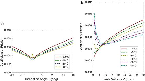

  

  (a) Relation between the coefficient of friction and the blade inclination angle (positive angles indicate inside edge), varying the temperature of ice; (b) average coefficient of friction during a stroke function of the skate velocity V (positive angles indicate inside edge), varying the temperature of ice. Both the plots refer to standard conditions: $T_{i} = -5\,^{\circ }$ C, skate speed V = 12 m s⁻¹, skater mass m = 75 kg, blade rocker radius r = 25 m, blade width w = 1. 1 mm. Adapted from [63]

• Figure 8.18b illustrates the relation between the coefficient of friction and the skate velocity (results are averaged over a range of blade inclination angle varying from − 20^∘ and 40^∘, typical of a skating stroke). In general it is possible to notice that temperature dependence of the ice friction coefficient is different at low and high velocities. According to the model, at higher velocities a warmer ice presents an higher coefficient of friction, while at lower velocities a warmer ice is “faster” (low coefficient of friction). Hence, according to the model, very fast skaters (in high level competitions velocities around 16 m s⁻¹ can be reached) will experience lower ice friction with colder ice, while slow skaters will experience lower ice friction with warmer ice [63]. Around 6 and 10 m s⁻¹, it is possible to find optimum values for the average friction coefficient: these results are comparable with the ones of De Koning et al. [34].

• Results of the model were compared with the measurements performed by De Koning et al. [34], made with a skater of 72 kg (really close to the standard mass of 75 kg here considered) and skate velocity of 8 m s⁻¹. In Fig. 8.19a the model and experimental values of friction coefficient are remarkably similar when averaged over all ice surface temperatures. The model does not simulate the systematic behavior seen in the experiments, with a minimum at − 7 ^∘C. Also in Fig. 8.19b the results are qualitatively comparable, even though the model underestimates the increase of ice friction with increasing skating speed. Authors suppose the discrepancy depends on the hypothesis of neglecting the thrust force [63].

  Fig. 8.19

  

  (a) Average ice friction coefficient during a skating stroke, function of ice surface temperature with a skate speed of 8 m s⁻¹; (b) average ice friction coefficient during a skating stroke, function of skate velocity with an ice surface temperature of − 4. 6 ^∘C. Standard conditions are used. Adapted from [63]

8.4.3.10 Conclusions

The FAST2.0i here presented is one of the most recent and complete models for ice friction of a speed skater. An interested reader can check the good results of this approach compared with numerical and experimental results in [63]. This model has some lacks and must respect numerous hypotheses. In particular, further developments may expand the validity of this formulation. The thrust is neglected, while it could be introduced using a biomechanical model of the skater. Again, a model of this kind can be useful to consider a potential moment exerted by the skater on the blade. Squeeze flow and heat flow models can be extended, e.g. including the y and z directions and the heat conduction between blade and ice (see also [89]).

References

Wikipedia -speed skating (May 2014). http://en.wikipedia.org/wiki/Speed_skating
D.L. Bird, Skating a brief history of ice and the national ice skating association of great Britain (May 2014). http://www.iceskating.org.uk/about/history
Wikipedia -Edinburgh skating club (May 2014). http://en.wikipedia.org/wiki/Edinburgh_Skating_Club
The edinburgh skating-club, with diagrams of figures and a list of the members. Edinburgh skating club (1865). http://books.google.it/books?id=8CQ7MwEACAAJ
Wikipedia -international skating union (May 2014). http://en.wikipedia.org/wiki/International_Skating_Union
The international skating union (ISU) (May 2014). http://www.isu.org/en/home
Special regulations and technical rules -speed skating and short track speed skating. As accepted by the 54th Ordinary Congress June 2012. International Skating Union (ISU) (2012)
Olympic -speed skating equipment and history (May 2014). http://www.olympic.org/speed-skating-equipment-andhistory?tab=equipment
Wikipedia -clap skate, May 2014. http://it.wikipedia.org/wiki/Clap_skate
G.J. Van Ingen Schenau et al., Skate, more particularly ice-skate for speed skating. EP Patent App. EP19,860,200,279, 1986. https://www.google.com/patents/EP0192312A2?cl=en
A. Shum, Clap skate with spring and cable biasing system. US Patent 6,007,075, 1999. http://www.google.com/patents/US6007075
T. Martin, Evolution of ice rinks. ASHRAE J. 46(11), S24–S30 (2004)
G. McCourt, S.L. Goodrich, Calgary’s olympic oval (Canada). Industria Italiana del Cemento 59(9), 524–543 (1989)
S.S. Jensen, Ice skating rink at the brisbane bicentenary sports and entertainment complex: Boondall Queensland. Aust. Refrig. Air Cond. Heat. 40(8), 23–24, 28 (1986)
K. Tusima et al., Development of a high speed skating rink by the control of the crystallographic plane of ice. Jpn. J. Tribol. 45, 17–26 (2000)
C. C\(\hat{a}\) mpian, M. Cristujiu, I. Benke, The supporting steel structure of the ice rink—city of T\(\hat{a}\) rgu Mureş, Romania Zs. Nagy, in Structures & Architecture, ed. by P.J.S. Cruz. ICSA 2010 – 1st International Conference on Structures & Architecture, 21–23 July 2010, Guimaraes (CRC Press, 2010), pp. 167–168
M. Schulitz, J. Güsgen, J. Kaußen, Ice skating and swimming stadium Lentpark in Cologne [Eis-und Schwimmstadion Lentpark in Köln] Stahlbau 83(1), 57–60 (2014)
Anon, roofing of an artificial ice skating rink. [Couverture D’UNE Patinoire Artificielle Ueberdachung Der Kunsteisbahn Arosa (CH).] Acier English ed. 44(4), 153–155 (1979)
www.scopus.com, Stadiums and arenas: a grandstand construction for German ice rink. Concr. Eng. Int. 11(1), 42–43 (2007)
Z. Nagy, I. Mircea Cristutiu, Advanced nonlinear investigations of a 50 m span frame case study: the steel structure of the ice rink, city of Targu-Mures, Romania, vol. 2, cited by (since 1996)1. 2010, pp. 649–656
A. Zak, O. Sikula, M. Trcala, Analysis of local moisture increase of timber constructions on ice arena roof. Adv. Mater. Res. 649, 291–294 (2013)
T. Davis, S. Kneisel, Building control systems at three new arenas. Can. Consult. Eng. (1995). www.scopus.com
H. Guo, S.C. Lee, L.Y. Chan, Indoor air quality in ice skating rinks in Hong Kong. Environ. Res. 94(3), 327–335 (2004)
J. Matsuo, T. Nagai, A. Sagae, M. Nakamura, S. Shimizu, T. Fujimoto, F. Maeda, Thermal characteristics and energy conservation measures in an indoor speed-skating arena. Paper presented at the Proceedings of Building Simulation 2011: 12th Conference of International Building Performance Simulation Association (2011), pp. 2072–2079
G. Teyssedou, R. Zmeureanu, D. Giguère, Thermal response of the concrete slab of an indoor ice rink (rp-1289). HVAC R Res. 15(3), 509–523 (2009)
G. Teyssedou, R. Zmeureanu, D. Giguère, Benchmarking model for the ongoing commissioning of the refrigeration system of an indoor ice rink. Autom. Constr. 35, 229–237 (2013)
Real world physics problems: physics of ice skating (June 2014). http://www.real-world-physics-problems.com/physics-of-ice-skating.html
D.M. Fintelman, O. den Braver, A.L. Schwab, A simple 2-dimensional model of speed skating which mimics observed forces and motions, in Multibody Dynamics 2011, ECCOMAS Thematic Conference, 2011
H. Houdijk et al., Push-off mechanics in speed skating with conventional skates and klapskates. Med. Sci. Sports Exerc. 32(3), 635–641 (2000)
G.J. Van Ingen Schenau, R.W. De Boer, G. De Groot, On the technique of speed skating. Int. J. Sport Biomech. 3, 419–431 (1987)
G.J. Van Ingen Schenau, R.W. de Boer, G. de Groot, The control of speed in elite female speed skaters. J. Biomech. 18, 91–96 (1985)
J.J. De Koning, Biomechanical aspects of speed skating. Ph.D. thesis, Vrije Universiteit, Faculty of Human Movement Sciences, Amsterdam, 1991
M.R. Yeadon, A method for obtaining three-dimensional data on ski jumping using pan and tilt cameras. Int. J. Sport Biomech. 5, 238–247 (1989)
J.J. De Koning, G. De Groot, G.J. van Ingen Schenau, Ice friction during speed skating. J. Biomech. 25, 565–571 (1992)
H. Jobse et al., Measurement of the push-off force and ice friction during speed skating. Int. J. Sport Biomech. 6, 92–100 (1990)
J.J. De Koning et al., From biomechanical theory to application in top sports: the Klapskate story. J. Biomech. 33, 1225–1229 (2000)
G.J. Van Ingen Schenau et al., A new skate allowing powerful plantar flexions improves performance. Med. Sci. Sports Exerc. 28, 531–535 (1996)
J.J. De Koning, G. De Groot, G.J. van Ingen Schenau, Coordination of leg muscles during speed skating. J. Biomech. 24(2), 137–146 (1991)
T.L. Allinger, A.J. Bogert, Skating technique for the straights, based on the optimization of a simulation model. Med. Sci. Sports Exerc. 29(2), 279–286 (1997)
J.J. De Koning, G.J. van Ingen Schenau, Performance-determining factors in speed skating, in Biomechanics in Sport: Performance Enhancement and Injury Prevention: Olympic Encyclopaedia of Sports Medicine, ed. by V. Zatsiorsky, vol. IX (Blackwell Science Ltd, Oxford, 2000), pp. 232–246. doi:http://dx.doi.org/10.1002/9780470693797.ch11.
E. Otten, Inverse and forward dynamics: models of multi-body systems. Philos. Trans. R. Soc. Lond. 358, 1493–1500 (2003)
P. Mantegazza, P. Masarati, Analysis of Systems of Differential-Algebraic Equations (DAE). Lecture Notes of Graduate Course on “Multibody System Dynamics” (22 November 2012)
R.W. de Boer, K.L. Nislen, The gliding and push-off technique of male and female olympic speed skaters. J. Appl. Biomech. 5(2), 119–134 (1989)
J.J. De Koning, G. de Groot, G.J. van Ingen Schenau, A power equation for the sprint in speed skating. J. Biomech 25, 573–580 (1992)
J.J. De Koning, G.J. van Ingen Schenau, On the estimation of mechanical power in endurance sports. Sport Sci. Rev. 3, 34–54 (1994)
J.J. De Koning, G.J. van Ingen Schenau, Performance-determining factors in speed skating, in Biomechanics in Sport, ed. by V.M. Zatsiorsky (Blackwell Science Ltd., Oxford, 2008)
G.J. Van Ingen Schenau, J.J. De Koning, G. De Groot, A simulation of speed skating performances based on a power equation. Med. Sci. Sports. Exerc. 22, 718–728 (1990)
J.J. De Koning et al., Experimental evaluation of the power balance model of speed skating. J. Appl. Physiol. 98(1), 227–233 (2004)
T.J. Barstow, P.A. Mole, Linear and nonlinear characteristics of oxygen uptake kinetics during heavy exercise. J. Appl. Physiol. 71, 2099–2106 (1991)
C. Foster et al., Pattern of energy expenditure during simulated competition. Med. Sci. Sports Exerc. 35, 826–831 (2003)
G.J. van Ingen Schenau, G. De Groot, A.P. Hollander, Some technical, physiological and anthropometrical aspects of speed skating. Eur. J. Appl. Physiol. Occup. Physiol. 50(3), 343–354 (1983)
G.J. van Ingen Schenau, The influence of air friction in speed skating. J. Biomech. 15(6), 449–58 (1982)
A. D’Auteuil, G. Larose, S. Zan, The effect of motion on wind tunnel drag measurement for athletes. Procedia Eng. 34, 62–67 (2012)
A. D’Auteuil, G.L. Larose, S.J. Zan, Relevance of similitude parameters for drag reduction in sport aerodynamics. Procedia Eng. 2, 2393–2398 (2010)
A. D’Auteuil et al., Detection of the boundary layer transition for non-circular cross-sections using surface pressure measurements, in Proceedings of the 13th International Conference on Wind Engineering, Amsterdam, 2011
M.M. Zdravkovich, Flow Around Circular Cylinders Volume 1: Fundamentals (Oxford Science Publications, New York, 1997)
S.J. Zan, K. Matsuda, Steady and unsteady loading on a roughened circular cylinder at Reynolds numbers up to 900,000. J. Wind Eng. Ind. Aerodyn. 90, 567–58 (2002)
A. D’Auteuil, G. Larose, S. Zan, Wind turbulence in speed skating: measurement, simulation and its effect on aerodynamic drag. J. Wind Eng. Ind. Aerodyn. 104–106, 585–593 (2012)
L.W. Brownlie et al., Reducing the aerodynamic drag of sports apparel: development of the Nike Swift sprint running and SwiftSkin speed skating suits, in The Engineering of Sport 5 (ISEA, Sheffield, 2004), pp. 90–96
G.H. Kuper, E. Sterken, Do skin suits increase average skating speed? Technical Report. University of Groningen, 2008
L.W. Brownlie, C.R. Kyle. Evidence that skin suits affect long track speed skating performance. Procedia Eng. 34, 26–31 (2012)
R. Rosenberg, Why is ice slippery? Phys. Today 58(12), 50–55 (2005)
E.P. Lozowski, K. Szilder, S. Maw, A model of ice friction for a speed skate blade. Sports Eng. 16(4), 239–253 (2013)
A.M. Kietzig, S.G. Hatzikiriakos, P. Englezos, Physics of ice friction. J. Appl. Phys. 107, 08110 (2010)
P. Barnes, D. Tabor, Plastic flow and pressure melting in the deformation of ice I. Nature 210, 878–882 (1966)
F.P. Bowden, T.P. Hughes, The mechanism of sliding on ice and snow. Proc. R. Soc. Lond. A 172(949), 280–298 (1939)
F.P. Bowden, Friction on snow and ice. Proc. R. Soc. Lond. A 217, 462–478 (1953)
M.J. Furey, Friction, wear and lubrication, in Chemistry and Physics of Interfaces II (American Chemical Society Publications, Washington, 1971)
V.F. Petrenko, R.W. Whitworth, Physics of Ice (Oxford University Press, Oxford, 1999), p. 373
P.V. Hobbs, Ice Physics (Clarendon Press, Oxford, 1974)
N.H. Fletcher, Surface structure of water and ice. Philos. Mag. 7, 255–59 (1962)
N.H. Fletcher, Surface structure of water and ice: II. A revised model. Philos. Mag. 18, 1287–1300 (1968)
R. Lacmann, I.N. Stranski, The growth of snow crystals. J. Cryst. Growth 13–14(C), 236–240 (1972)
J.G. Dash, F. Haiying, J.S. Wettlaufer. The premelting of ice and its environmental consequences. Rep. Prog. Phys. 58, 115 (1995)
L. Makkonen, Surface melting of ice. J. Phys. Chem. B 101(32), 6196–6200 (1997)
N. Fukuta, J. Phys. (Paris) 48, 503 (1987)
G.-J. Kroes, Surface melting of the (0001) face of {TIP4P} ice. Surf. Sci. 275(3), 365–382 (1992). ISSN: 0039-6028. doi: http://dx.doi.org/10.1016/0039-6028(92)90809-K. http://www.sciencedirect.com/science/article/pii/003960289290809K
J.P. Devlin, V. Buch, Surface of ice as viewed from combined spectroscopic and computer modeling studies. J. Phys. Chem. 99(45), 16534–16548 (1995)
Y. Furukawa, H. Nada, Anisotropic surface melting of an ice crystal and its relationship to growth forms. J. Phys. Chem. B 101(32), 6167–6170 (1997)
N. Materer et al., Molecular surface structure of ice(0001): dynamical low-energy electron diffraction, total-energy calculations and molecular dynamics simulations. Surf. Sci. 381(2–3), 190–210 (1997)
F.P. Bowden, Introduction to the discussion: the mechanism of friction. Proc. R. Soc. Lond. A Math. Phys. Sci. 212, 440–449 (1952)
B.N.J. Persson, Sliding Friction. Physical Principles and Applications, 2nd edn. (Springer, Berlin, 2000)
B. Bhusam, Introduction to Tribology (Wiley, New York, 2002)
F.P. Bowden, D. Tabor, The Friction and Lubrication of Solids (Oxford University Press, Oxford, 1964)
V.F. Petrenko, R.W. Whitworth, Physics of Ice (Oxford University Press, Oxford, 1999)
S.C. Colbeck, Kinetic friction of snow. J. Glaciol. 34(116), 78–86 (1988)
A.-M. Kietzig, S.G. Hatzikiriakos, P. Englezos, Ice friction: the effects of surface roughness, structure and hydrophobicity. J. Appl. Phys. 106 024303 (2009)
A. Penny et al., Speedskate ice friction: review and numerical model -FAST 1.0, in Physics and Chemistry of Ice, ed. by W.F. Kuhs. R. Soc. Chem. (2007), pp. 495–504. doi:10.1039/9781847557773
E.P. Lozowski, K. Szilder, Derivation and new analysis of a hydrodynamic model of speed skate ice friction. Int. J. Offshore Polar Eng. 23, 104–111 (2013)
L. Poirier et al., Getting a grip on ice friction, in Proceedings of the Twenty-first (2011) International Offshore and Polar Engineering Conference, Maui, HI, 19–24 June 2011
E.P. Lozowski, K. Szilder, S. Maw, A model of ice friction for an inclined incising slider, in The Twenty-second International Offshore and Polar Engineering Conference. International Society of Offshore and Polar Engineers (2012), pp. 1243–1251
Author information
Authors and Affiliations
Corresponding author
Editor information
Editors and Affiliations
Rights and permissions
Copyright information
© 2016 The Editor
About this chapter
Cite this chapter
Belloni, E., Sabbioni, E., Melzi, S. (2016). Ice Skating. In: Braghin, F., Cheli, F., Maldifassi, S., Melzi, S., Sabbioni, E. (eds) The Engineering Approach to Winter Sports. Springer, New York, NY. https://doi.org/10.1007/978-1-4939-3020-3_8
Download citation
DOI: https://doi.org/10.1007/978-1-4939-3020-3_8
Publisher Name: Springer, New York, NY
Print ISBN: 978-1-4939-3019-7
Online ISBN: 978-1-4939-3020-3
eBook Packages: EngineeringEngineering (R0)