Planarity

Abstract

The study of planar and nonplanar graphs and, in particular, the several attempts to solve the four-color conjecture have contributed a great deal to the growth of graph theory. Actually, these efforts have been instrumental to the development of algebraic, topological, and computational techniques in graph theory.

These keywords were added by machine and not by the authors. This process is experimental and the keywords may be updated as the learning algorithm improves.

8.1 Introduction

The study of planar and nonplanar graphs and, in particular, the several attempts to solve the four-color conjecture have contributed a great deal to the growth of graph theory. Actually, these efforts have been instrumental to the development of algebraic, topological, and computational techniques in graph theory.

In this chapter, we present some of the basic results on planar graphs. In particular, the two important characterization theorems for planar graphs, namely, Wagner’s theorem (same as the Harary–Tutte theorem) and Kuratowski’s theorem, are presented. Moreover, the nonhamiltonicity of the Tutte graph on 46 vertices (see Fig. 8.28 and also the front wrapper) is explained in detail.

8.2 Planar and Nonplanar Graphs

Definition 8.2.1.

A graph G is planar if there exists a drawing of G in the plane in which no two edges intersect in a point other than a vertex of G, where each edge is a Jordan arc (that is, a simple arc). Such a drawing of a planar graph G is called a plane representation of G. In this case, we also say that G has been embedded in the plane. A plane graph is a planar graph that has already been embedded in the plane.

Example 8.2.2.

There exist planar as well as nonplanar graphs. In Fig. 8.1, a planar graph and two of its plane representations are shown. Note that all trees are planar as also are cycles and wheels. The Petersen graph is nonplanar (a proof of this result will be given in the subsequent paragraphs).

Fig. 8.1

A planar graph with two plane embeddings

Before proceeding further, let us recall here the celebrated Jordan curve theorem. If J is any closed Jordan curve in the plane, the complement of J (with respect to the plane) is partitioned into two disjoint open connected subsets of the plane, one of which is bounded and the other unbounded. The bounded subset is called the interior of J and is denoted by int J. The unbounded subset is called the exterior of J and is denoted by ext J. The Jordan curve theorem (of topology) states that if J is any closed Jordan curve in the plane, any arc joining a point of int J and a point of ext J must intersect J at some point (see Fig. 8.2) (the proof of this result, although intuitively obvious, is tedious).

Fig. 8.2

Arc connecting point x in int J with point y in ext J

Let G be a plane graph. Then the union of the edges (as Jordan arcs) of a cycle C of G form a closed Jordan curve, which we also denote by C. A plane graph G divides the rest of the plane (i.e., plane minus the edges and vertices of G), say π, into one or more faces, which we define below. We define an equivalence relation ∼ on π. 

Definition 8.2.3.

We say that for points A and B of π, A ∼ B if and only if there exists a Jordan arc from A to B in π. Clearly, ∼ is an equivalence relation on π. The equivalence classes of the above equivalence relation are called the faces of G. 

Remark 8.2.4.

• 1. We claim that a connected graph is a tree if and only if it has only one face. Indeed, since there are no cycles in a tree T, the complement of a plane embedding of T in the plane is connected (in the above sense), and hence a tree has only one face. Conversely, it is clear that if a connected plane graph has only one face, then it must be a tree.

• 2. Any plane graph has exactly one unbounded face. The unbounded face is also referred to as the exterior face of the plane graph. All other faces, if any, are bounded. Figure 8.3 represents a plane graph with seven faces.

The distinction between bounded and unbounded faces of a plane graph is only superfluous, as there exists a plane representation G ₁ of a plane graph G in which any specified face of G ₁ becomes the unbounded face, as is shown below. (This of course means that there exists a plane representation of G such that any specified vertex or edge belongs to the unbounded face.) We consider embeddings of a graph on a sphere. A graph is embeddable on a sphereS if it can be drawn on the surface of S so that its edges intersect only at its vertices. Such a drawing, if it exists, is called an embedding of G on S. Embeddings on a sphere are called spherical embeddings. What we have given here is only a naive definition. For a more rigorous description of spherical embeddings, see [79].

Fig. 8.3

A plane graph with seven faces

To prove the next theorem, we need to recall the notion of stereographic projection. Let S be a sphere resting on a plane P so that P is a tangent plane to S. Let N be the “north pole,” the point on the sphere diametrically opposite the point of contact of S and P. Let the straight line joining N and a point s of S ∖ {N} meet P at p. Then the mapping η : S ∖ {N} → P defined by η(s) = p is called the stereographic projection of S from N (see Fig. 8.4).

Fig. 8.4

Stereographic projection of the sphere S from N

Theorem 8.2.5.

A graph is planar if and only if it is embeddable on a sphere.

Proof.

Let a graph G be embeddable on a sphereand let G′ be a spherical embedding of G. The image of G′ under the stereographic projection η of the sphere from a point N of the sphere not on G′ is a plane representation of G on P. Conversely, if G′ is a plane embedding of G on a plane P, then the inverse of the stereographic projection of G′ on a sphere touching the plane P gives a spherical embedding of G.

Theorem 8.2.6.

• (a) Let G be a plane graph and f be a face of G. Then there exists a plane embedding of G in which f is the exterior face.

• (b) Let G be a planar graph. Then G can be embedded in the plane in such a way that any specified vertex (or edge) belongs to the unbounded face of the resulting plane graph.

Proof.

• (a) Let n be a point of int f. Let G′ = σ(G) be a spherical embedding of G and let N = σ(n). Let η be the stereographic projection of the sphere with N as the north pole. Then the map ησ (σ followed by η) gives a plane embedding of G that maps f onto the exterior face of the plane representation (ησ)(G) of G. 

• (b) Let f be a face containing the specified vertex (respectively, edge) in a plane representation of G. Now, by part (a) of the theorem, there exists a plane embedding of G in which f becomes the exterior face. The specified vertex (respectively, edge) then becomes a vertex (respectively, edge) of the new unbounded face.

Remark 8.2.7.

• 1. Let G be a connected plane graph. Each edge of G belongs to one or two faces of G. A cut edge of G belongs to exactly one face, and conversely, if an edge belongs to exactly one face of G, it must be a cut edge of G. An edge of G that is not a cut edge belongs to exactly two faces and conversely.

• 2. The union of the vertices and edges of G incident with a face f of G is called the boundary of f and is denoted by b(f). The vertices and edges of a plane graph G belonging to the boundary of a face of G are said to be incident with that face. If G is connected, the boundary of each face is a closed walk in which each cut edge of G is traversed twice. When there are no cut edges, the boundary of each face of G is a closed trail in G. (See, for instance, face f ₁ of Fig. 8.3.) However, if G is a disconnected plane graph, then the edges and the vertices incident with the exterior face will not define a trail.

• 3. The number of edges incident with a face f is defined as the degree of f. In counting the degree of a face, a cut edge is counted twice. Thus, each edge of a plane graph G contributes two to the sum of the degrees of the faces. It follows that if $\mathcal{F}$ denotes the set of faces of a plane graph G, then $\sum \limits_{f\in \mathcal{F}}^{} d(f) = 2m(G),$ where d(f) denotes the degree of the face f. 

In Fig. 8.5, d(f ₁) = 3, d(f ₂) = 9, d(f ₃) = 6, and d(f ₄) = 8. 

Fig. 8.5

Plane graph with four faces

Theorem 8.2.8 connects the planarity of G with the planarity of its blocks.

Theorem 8.2.8.

A graph G is planar if and only if each of its blocks is planar.

Proof.

If G is planar, then each of its blocks is planar, since a subgraph of a planar graph is planar. Conversely, suppose that each block of G is planar. We now use induction on the number of blocks of G to prove the result. Without loss of generality, we assume that G is connected. If G has only one block, then G is planar.

Now suppose that G has k planar blocks and that the result is true for all connected graphs having (k − 1) planar blocks. Choose any end block B ₀ of G and delete from G all the vertices of B ₀ except the unique cut vertex, say v ₀, of G in B ₀. The resulting connected subgraph G′ of G contains (k − 1) planar blocks. Hence, by the induction hypothesis, G′ is planar. Let $\tilde{{G}^{{\prime}}}$ be a plane embedding of G′ such that v ₀ belongs to the boundary of the unbounded face, say f′ (refer to Theorem 8.2.6). Let $\tilde{{B}}_{0}$ be a plane embedding of B ₀ in f′ so that v ₀ is in the boundary of the exterior face of $\tilde{{B}}_{0}.$ Then (by the identification of v ₀ in the two embeddings), $\tilde{{G}^{{\prime}}}\cup \tilde{ {B}}_{0}$ is a plane embedding of G.

Remark 8.2.9.

In testing for the planarity of a graph G, one may delete multiple edges and loops of G, if any. This is so because if a graph H is nonplanar, the removal of loops and parallel edges of H results in a subgraph of H, which is also nonplanar. Also, by Theorem 8.2.8, G can be assumed to be a block and hence 2-connected. If G has a vertex of degree 2, say v ₀, and vv ₀ v′ is the path formed by the two edges incident with v ₀, contraction of vv ₀ and deletion of the multiple edges (if any) thus formed again result in a planar graph. Let G′ be the graph obtained from G by performing such contractions successively at vertices of degree 2 and deleting the resulting multiple edges. Then G is planar if and only if G′ is planar. From these observations, it is clear that in designing a planarity algorithm (i.e., an algorithm to test planarity), it suffices to consider only 2-connected simple graphs with minimum degree at least 3. (For a planarity algorithm, see [49].)

Exercise 2.1.

Show that every graph with at most three cycles is planar.

Exercise 2.2.

Find a simple graph G with degree sequence (4, 4, 3, 3, 3, 3) such that

• (a) G is planar.

• (b) G is nonplanar.

Exercise 2.3.

Redraw the following planar graph so that the face f becomes the exterior face.

8.3 Euler Formula and Its Consequences

We have noted that a planar graph may have more than one plane representation (see Fig. 8.1). A natural question that would arise is whether the number of faces is the same in each such representation. The answer to this question is provided by the Euler formula.

Theorem 8.3.1 (Euler formula). 

For a connected plane graph G, n − m + f = 2, where n, m, and f denote the number of vertices, edges, and faces of G, respectively.

Proof.

We apply induction on f.

If f = 1, then G is a tree and m = n − 1. Hence, n − m + f = 2. 

Now assume that the result is true for all plane graphs with f − 1 faces, f ≥ 2, and suppose that G has f faces. Since f ≥ 2, G is not a tree, and hence contains a cycle C. Let e be an edge of C. Then e belongs to exactly two faces, say f ₁ and f ₂, of G and the deletion of e from G results in the formation of a single face from f ₁ and f ₂ (see Fig. 8.5). Also, since e is not a cut edge of G, G − e is connected. Further, the number of faces of G − e is f − 1. So applying induction to G − e, we get n − (m − 1) + (f − 1) = 2, and this implies that n − m + f = 2. This completes the proof of the theorem.

Below are some of the consequences of the Euler formula.

Corollary 8.3.2.

All plane embeddings of a given planar graph have the same number of faces.

Proof.

Since f = m − n + 2, the number of faces depends only on n and m, and not on the particular embedding.

Corollary 8.3.3.

If G is a simple planar graph with at least three vertices, then m ≤ 3n − 6.

Proof.

Without loss of generality, we can assume that G is a simple connected plane graph. Since G is simple and n ≥ 3, each face of G has degree at least 3. Hence, if $\mathcal{F}$ denotes the set of faces of G, ${\sum \nolimits }_{f\in \mathcal{F}}d(f) \geq 3\mathrm{f}.$ But ${\sum \nolimits }_{f\in \mathcal{F}}d(f) = 2m.$ Consequently, $2m \geq 3\mathrm{f},$ so that $\mathrm{f} \leq \frac{2m} {3}.$

By the Euler formula, m = n + f − 2. Now $\mathrm{f} \leq \frac{2m} {3}$ implies that $m \leq n + \left (\frac{2m} {3} \right ) - 2.$ This gives m ≤ 3n − 6.

The above result is not valid if n = 1 or 2. Also, the condition of Corollary 8.3.3 is not sufficient for the planarity of a simple connected graph, as the Petersen graph shows. For the Petersen graph, m = 15, n = 10, and hence m ≤ 3n − 6, but the graph is not planar (see Corollary 8.3.7 below).

Example 8.3.4.

Show that the complement of a simple planar graph with 11 vertices is nonplanar.

Solution.

Let G be a simple planar graph with n(G) = 11. Since G is planar, m(G) ≤ 3n − 6 = 27. If G ^c were also planar, then m(G ^c) ≤ 3n − 6 = 27. On the one hand, m(G) + m(G ^c) ≤ 27 + 27 = 54, whereas, on the other hand, $m(G) + m({G}^{c}) = m({K}_{11}) = \left( \mathop{} \limits_2^{11}\right) = 55.$ Hence, we arrive at a contradiction. This contradiction proves that G ^c is nonplanar.

Corollary 8.3.5.

For any simple planar graph G, δ(G) ≤ 5.

Proof.

If n ≤ 6, then Δ(G) ≤ 5. Hence, δ(G) ≤ Δ(G) ≤ 5, proving the result for such graphs. So assume that n ≥ 7. By Corollary 8.3.3, m ≤ 3n − 6. Now, $\delta n \leq {\sum \nolimits }_{v\in V (G)}{d}_{G}(v) = 2m \leq 2(3n - 6) = 6n - 12.$ Hence, n(δ − 6) ≤ − 12. Consequently, δ − 6 is negative, implying that δ ≤ 5.

Recall that the girth of a graph G is the length of a shortest cycle in G. 

Theorem 8.3.6.

If the girth k of a connected plane graph G is at least 3, then $m \leq \frac{k(n-2)} {(k-2)}.$

Proof.

Let $\mathcal{F}$ denote the set of faces and f, as before, denote the number of faces of G. If $f \in \mathcal{F},$ then d(f) ≥ k. Since $2m ={ \sum \nolimits }_{f\in \mathcal{F}}d(f),$ we get 2m ≥ kf. By Theorem 8.3.1, f = 2 − n + m. Hence, 2m ≥ k(2 − n + m), implying that m(k − 2) ≤ k(n − 2). Thus, $m \leq \frac{k(n-2)} {(k-2)}$.

Corollary 8.3.7.

The Petersen graph P is nonplanar.

Proof.

The girth of the Petersen graph P is 5, n(P) = 10, and m(P) = 15. Hence, if P were planar, $15 \leq \frac{5(10-2)} {5-2}$, which is not true. Hence, P is nonplanar.

Exercise 3.1.

Show that every simple bipartite cubic planar graph contains a C ₄. 

Exercise 3.2.

A nonplanar graph G is called planar-vertex-critical if G − v is planar for every vertex v of G. Prove that a planar-vertex-critical graph must be 2-connected.

Exercise 3.3.

Verify Euler’s formula for the following plane graph.

Exercise 3.4.

Let G be a simple plane cubic graph having eight faces. Determine n(G). Draw two such graphs that are nonisomorphic.

Exercise 3.5.

Prove that if G is a simple connected planar bipartite graph, then m ≤ 2n − 4, where n ≥ 3. 

Exercise 3.6.

Prove that a simple planar graph (with at least four vertices) has at least four vertices each of degree 5 at most.

Exercise 3.7.

If G is a nonplanar graph, show that it has either five vertices of degree at least 4, or six vertices of degree at least 3.

Exercise 3.8.

Prove that a simple planar graph with minimum degree at least five contains at least 12 vertices. Give an example of a simple planar graph on 12 vertices with minimum degree 5.

Exercise 3.9.

Show that there is no 6-connected planar graph.

Exercise 3.10.

Let G be a plane graph of order n and size m in which every face is bounded by a k-cycle. Show that $m = \tfrac{k(n-2)} {(k-2)}$.

Definition 8.3.8.

A graph G is maximal planar if G is planar, but for any pair of nonadjacent vertices u and v of G, G + uv is nonplanar.

Remark 8.3.9.

Any planar graph is a spanning subgraph of a maximal planar graph. Indeed, if $\tilde{G}$ is a plane embedding of a planar graph G with at least three vertices, and if e = uv is a cut edge of $\tilde{G}$ embedded in a face f of $\tilde{G},$ it is clear that there exists a vertex w on the boundary of f such that the edge uw or vw can be drawn in f so that either $\tilde{G} + (vw)$ or $\tilde{G} + (uw)$ is also a plane graph (see Fig. 8.6a). Further, if C ₀ is any cycle bounding a face f ₀ of a plane graph H, then edges can be drawn in int C ₀ without crossing each other so that f ₀ is divided into triangles (see Fig. 8.6b).

Fig. 8.6

Procedure to get maximal planar graphs

Definition 8.3.10.

A plane triangulation is a plane graph in which each of its faces is bounded by a triangle. A plane triangulation of a plane graph G is a plane triangulation H such that G is a spanning subgraph of H. 

Remark 8.3.11.

Remark 8.3.9 shows that a plane embedding of a simple maximal planar graph is a plane triangulation.

Note that any simple plane graph is a subgraph of a simple maximal plane graph and hence is a spanning subgraph of some plane triangulation. Thus, to any simple plane graph G that is not already a plane triangulation, we can add a set of new edges to obtain a plane triangulation. The set of new edges thus added need not be unique.

Figure 8.7a is a simple plane graph G and Fig. 8.7b is a plane triangulation of G; Fig. 8.7c is a plane triangulation of G isomorphic to the graph of Fig. 8.7b having only straight-line edges. (A result of Fáry [60] states that every simple planar graph has a plane embedding in which each edge is a straight line.)

Fig. 8.7

(a) Graph G and (b), (c) are plane triangulations of G

Exercise 3.11.

Embed the 3-cube Q ₃ (see Exercise 4.4 of Chap. 5) in a maximal planar graph having the same vertex set as Q ₃. Count the number of new edges added.

Exercise 3.12.

Prove that for a simple maximal planar graph on n ≥ 3 vertices, m = 3n − 6. 

Exercise 3.13.

Use Exercise 3.12 to show that for any simple planar graph, m ≤ 3n − 6. 

Exercise 3.14.

Show that every plane triangulation of order n ≥ 4 is 3-connected.

Exercise 3.15.

Let G be a maximal planar graph with n ≥ 4. Let n _i denote the number of vertices of degree i in G. Then prove that 3n ₃ + 2n ₄ + n ₅ = 12 + n ₇ + 2n ₈ + 3n ₉ + 4n ₁₀ + …. (Hint: Use the fact that n = n ₃ + n ₄ + n ₅ + n ₆ + …. )

Exercise 3.16.

Generalize the Euler formula for disconnected plane graphs.

8.4 K ₅ andK _3, 3 Are NonplanarGraphs

In this section we prove that K ₅ and K _3, 3 are nonplanar. These two graphs are basic in Kuratowski’s characterization of planar graphs (see Theorem 8.7.5 given later in this chapter). For this reason, they are often referred to as the two Kuratowski graphs.

Theorem 8.4.1.

K ₅ is nonplanar.

First proof. This proof uses the Jordan curve theorem. Assume the contrary, namely, K ₅ is planar. Let v ₁, v ₂, v ₃, v ₄, and v ₅ be the vertices of K ₅ in a plane representation of K ₅. The cycle C = v ₁ v ₂ v ₃ v ₄ v ₁ (as a closed Jordan curve) divides the plane into two faces, namely, the interior and the exterior of C. The vertex v ₅ must belong either to int C or to ext C. Suppose that v ₅ belongs to int C (a similar proof holds if v ₅ belongs to ext C). Draw the edges v ₅ v ₁, v ₅ v ₂, v ₅ v ₃, and v ₅ v ₄ in int C. Now there remain two more edges v ₁ v ₃ and v ₂ v ₄ to be drawn. None of these can be drawn in int C, since it is assumed that K ₅ is planar. Thus, v ₁ v ₃ lies in ext C. Then one of v ₂ and v ₄ belongs to the interior of the closed Jordan curve C ₁ = v ₁ v ₅ v ₃ v ₁ and the other to its exterior (see Fig. 8.8). Hence, v ₂ v ₄ cannot be drawn without violating planarity.

Fig. 8.8

Graph for first proof of Theorem 8.4.1

Remark 8.4.2.

The first proof of Theorem 8.4.1 shows that all the edges of K ₅ except one can be drawn in the plane without violating planarity. Hence, for any edge e of K ₅, K ₅ − e is planar.

If K ₅ were planar, it follows from Theorem 8.3.6 that $10 \leq \frac{3(5-2)}{(3-2)},$ which is not true. Hence, K ₅ is nonplanar.

Theorem 8.4.3.

K _3,3 is nonplanar.

The proof is by the use of the Jordan curve theorem. Suppose that K _3, 3 is planar. Let U = { u ₁, u ₂, u ₃} and V = { v ₁, v ₂, v ₃} be the bipartition of K _3, 3 in a plane representation of the graph. Consider the cycle C = u ₁ v ₁ u ₂ v ₂ u ₃ v ₃ u ₁. Since the graph is assumed to be planar, the edge u ₁ v ₂ must lie either in the interior of C or in its exterior. For the sake of definiteness, assume that it lies in int C (a similar proof holds if one assumes that the edge u ₁ v ₂ lies in ext C). Two more edges remain to be drawn, namely, u ₂ v ₃ and u ₃ v ₁. None of these can be drawn in int C without crossing the edge u ₁ v ₂. Hence, both of them are to be drawn in ext C. Now draw u ₂ v ₃ in ext C. Then one of v ₁ and u ₃ belongs to the interior of the closed Jordan curve C ₁ = u ₁ v ₂ u ₂ v ₃ u ₁ and the other to the exterior of C ₁ (see Fig. 8.9). Hence, the edge v ₁ u ₃ cannot be drawn without violating planarity. This shows that K _3, 3 is nonplanar.

Fig. 8.9

Graph for first proof of Theorem 8.4.3

Second proof. Suppose K _3, 3 is planar. Let f be the number of faces of G = K _3, 3 in a plane embedding of G and $\mathcal{F},$ the set of faces of G. As the girth of K _3, 3 is 4, we have $m = \frac{1} {2}{ \sum \nolimits }_{f\in \mathcal{F}}d(f) \geq \frac{4\mathrm{f}} {2} = 2\mathrm{f}.$ By Theorem 8.3.1, n − m + f = 2. For K _3, 3, n = 6, and m = 9. Hence, f = 2 + m − n = 5. Thus, 9 ≥ 2. 5 = 10, a contradiction.

Exercise 4.1.

Give yet another proof of Theorem 8.4.3.

Exercise 4.2.

Find the maximum number of edges in a planar complete tripartite graph with each part of size at least 2.

Remark 8.4.4.

As in the case of K ₅, for any edge e of K _3, 3, K _3, 3 − e is planar. Observe that the graphs K ₅ and K _3, 3 have some features in common.

• 1. Both are regular graphs.

• 2. The removal of a vertex or an edge from each graph results in a planar graph.

• 3. Contraction of an edge results in a planar graph.

• 4. K ₅ is a nonplanar graph with the smallest number of vertices, whereas K _3, 3 is a nonplanar graph with the smallest number of edges. (Hence, any nonplanar graph must have at least five vertices and nine edges.)

8.5 Dual of a Plane Graph

Let G be a plane graph. One can form out of G a new graph H in the following way. Corresponding to each face f of G, take a vertex f ^∗ and corresponding to each edge e of G, take an edge e ^∗. Then edge e ^∗ joins vertices f ^∗ and g ^∗ in H if and only if edge e is common to the boundaries of faces f and g in G. (It is possible that f may be the same as g. ) The graph H is then called the dual (or more precisely, the geometric dual) of G (see Fig. 8.10).

Fig. 8.10

A plane graph G and its dual H

If e is a cut edge of G embedded in face f of G, then e ^∗ is a loop at f ^∗. H is a planar graph, and there exists a natural way of embedding H in the plane. Vertex f ^∗, corresponding to face f, is placed in face f of G. Edge e ^∗, joining f ^∗ and g ^∗, is drawn so that e ^∗ crosses e once and only once and crosses no other edge. This procedure is illustrated in Fig. 8.11. This embedding is the canonical embedding of H. H with this canonical embedding is denoted by G ^∗. Any two embeddings of H, as described above, are isomorphic. The definition of the dual implies that m(G ^∗) = m(G), n(G ^∗) = f(G), and ${d}_{{G}^{{_\ast}}}({f}^{{_\ast}}) = {d}_{G}(f),$ where d _G (f) denotes the degree of the face f of G. 

Fig. 8.11

Procedure for drawing the dual graph

From the manner of construction of G ^∗, it follows that

• (i) An edge e of a plane graph G is a cut edge of G if and only if e ^∗ is a loop of G ^∗, and it is a loop of G if and only if e ^∗ is a cut edge of G ^∗.

• (ii) G ^∗ is connected whether G is connected or not (see graphs G and G ^∗ of Fig. 8.12).

  Fig. 8.12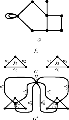

  

  A disconnected graph G and its (connected) dual G ^∗

The canonical embedding of the dual of G ^∗ is denoted by G ^∗ ∗. It is easy to check that G ^∗ ∗ is isomorphic to G if and only if G is connected. Graph isomorphism does not preserve duality; that is, isomorphic plane graphs may have nonisomorphic duals. The graphs G and H of Fig. 8.13 are isomorphic plane graphs, but G ^∗ ≄ H ^∗. G has a face of degree 5, whereas no face of H has degree 5. Hence, G ^∗ has a vertex of degree 5, whereas H ^∗ has no vertex of degree 5. Consequently, G ^∗ ≄ H ^∗. 

Exercise 5.1.

Draw the dual of

• (i) The Herschel graph (graph of Fig. 5.4).

• (ii) The graph G given below:

Exercise 5.2.

A plane graph G is called self-dual if G ≃ G ^∗. Prove the following:

• (i) All wheels W _n  (n ≥ 3) are self-dual.

• (ii) For a self-dual graph, 2n = m + 2. 

Exercise 5.3.

Construct two infinite families of self-dual graphs.

8.6 The Four-Color Theorem and the Heawood Five-Color Theorem

What is the minimum number of colors required to color the world map of countries so that no two countries having a common boundary receive the same color? This simple-looking problem manifested itself into one of the most challenging problems of graph theory, popularly known as the four-color conjecture (4CC).

Fig. 8.13

Isomorphic graphs G and H for which G ^∗ ≄ H ^∗

The geographical map of the countries of the world is a typical example of a plane graph. An assignment of colors to the faces of a plane graph G so that no two faces having a common boundary containing at least one edge receive the same color is a face coloring of G. The face-chromatic number χ^∗(G) of a plane graph G is the minimum k for which G has a face coloring using k colors. The problem of coloring a map so that no two adjacent countries receive the same color can thus be transformed into a problem of face coloring of a plane graph G. The face coloring of G is closely related to the vertex coloring of the dual G ^∗ of G. The fact that two faces of G are adjacent in G if and only if the corresponding vertices of G ^∗ are adjacent in G ^∗ shows that G is k-face-colorable if and only if G ^∗ is k-vertex-colorable.

It was young Francis Guthrie who conjectured, while coloring the district map of England, that four colors were sufficient to color the world map so that adjacent countries receive distinct colors. This conjecture was communicated by his brother to De Morgan in 1852. Guthrie’s conjecture is equivalent to the statement that any plane graph is 4-face-colorable. The latter statement is equivalent to the conjecture: Every planar graph is 4-vertex-colorable.

After the conjecture was first published in 1852, many attempted to settle it. In the process of settling the conjecture, many equivalent formulations of this conjecture were found. Assaults on the conjecture were made using such varied branches of mathematics as algebra, number theory, and finite geometries. The solution found the light of the day when Appel, Haken, and Koch [8] of the University of Illinois established the validity of the conjecture in 1976 with the aid of computers (see also [6,  7]). The proof includes, among other things, 10¹⁰ units of operations, amounting to a staggering 1200 hours of computer time on a high-speed computer available at that time.

Although the computer-oriented proof of Appel, Haken, and Koch settled the conjecture in 1976 and has stood the test of time, a theoretical proof of the four-color problem is still to be found.

Even though the solution of the 4CC has been a formidable task, it is rather easy to establish that every planar graph is 6-vertex-colorable.

Theorem 8.6.1.

Every planar graph is 6-vertex-colorable.

Proof.

The proof is by induction on n, the number of vertices of the graph. The result is trivial for planar graphs with at most six vertices. Assume the result for planar graphs with n − 1, n ≥ 7, vertices. Let G be a planar graph with n vertices. By Corollary 8.3.5, δ(G) ≤ 5, and hence G has a vertex v of degree at most 5. By hypothesis, G − v is 6-vertex-colorable. In any proper 6-vertex coloring of G − v, the neighbors of v in G would have used only at most five colors, and hence v can be colored by an unused color. In other words, G is 6-vertex-colorable.

It involves some ingenious arguments to reduce the upper bound for the chromatic number of a planar graph from 6 to 5. The upper bound 5 was obtained by Heawood [103] as early as 1890.

Theorem 8.6.2 (Heawood’s five-color theorem). 

Every planar graph is 5-vertex-colorable.

Proof.

The proof is by induction on n(G) = n. Without loss of generality, we assume that G is a connected plane graph. If n ≤ 5, the result is clearly true. Hence, assume that n ≥ 6 and that any planar graph with fewer than n vertices is 5-vertex-colorable. G being planar, δ(G) ≤ 5 by Corollary 8.3.5, and so G contains a vertex v ₀ of degree not exceeding 5. By the induction hypothesis, G − v ₀ is 5-vertex-colorable.

If d(v ₀) ≤ 4, at most four colors would have been used in coloring the neighbors of v ₀ in G in a 5-vertex coloring of G − v ₀. Hence, an unused color can then be assigned to v ₀ to yield a proper 5-vertex coloring of G. 

If d(v ₀) = 5, but only four or fewer colors are used to color the neighbors of v ₀ in a proper 5-vertex coloring of G − v ₀, then also an unused color can be assigned to v ₀ to yield a proper 5-vertex coloring of G. 

Hence, assume that the degree of v ₀ is 5 and that in every 5-coloring of G − v ₀, the neighbors of v ₀ in G receive five distinct colors. Let v ₁, v ₂, v ₃, v ₄, and v ₅ be the neighbors of v ₀ in a cyclic order in a plane embedding of G. Choose some proper 5-coloring of G − v ₀ with colors, say, c ₁, c ₂, …, c ₅. Let {V ₁, V ₂, …, V ₅} be the color partition of G − v ₀, where the vertices in V _i are colored c _i , 1 ≤ i ≤ 5. Assume further that v _i  ∈ V _i , 1 ≤ i ≤ 5. 

Let G _ij be the subgraph of G − v ₀ induced by V _i ∪V _j . Suppose v _i and v _j , 1 ≤ i, j ≤ 5, belong to distinct components of G _ij . Then the interchange of the colors c _i and c _j in the component of G _ij containing v _i would give a recoloring of G − v ₀ in which only four colors are assigned to the neighbors of v ₀. But this is against our assumption. Hence, v _i and v _j must belong to the same component of G _ij . Let P _i, j be a v _i -v _j path in G _ij . Let C denote the cycle v ₀ v ₁ P ₁₃ v ₃ v ₀ in G (Fig. 8.14). Then C separates v ₂ and v ₄; that is, one of v ₂ and v ₄ must lie in int C and the other in ext C. In Fig. 8.14, v ₂ ∈ int C and v ₄ ∈ ext C. Then P ₂₄ must cross C at a vertex of C. But this is clearly impossible since no vertex of C receives either of the colors c ₂ and c ₄. Hence, this possibility cannot arise, and G is 5-vertex-colorable.

Note that the bound 4 in the inequality χ(G) ≤ 4 for planar graphs G is best possible since K ₄ is planar and χ(K ₄) = 4. 

Fig. 8.14

Graph for proof of Theorem 8.6.2

Exercise 6.1.

Show that a planar graph G is bipartite if and only if each of its faces is of even degree in any plane embedding of G. 

Exercise 6.2.

Show that a connected plane graph G is bipartite if and only if G ^∗ is Eulerian. Hence, show that a connected plane graph is 2-face-colorable if and only if it is Eulerian.

Exercise 6.3.

Prove that a Hamiltonian plane graph is 4-face-colorable and that its dual is 4-vertex-colorable.

Exercise 6.4.

Show that a plane triangulation has a 3-face coloring if and only if it is not K ₄. (Hint: Use Brooks’ theorem.)

Remark 8.6.3.

(Grötzsch): If G is a planar graph that contains no triangle, then G is 3-vertex-colorable.

8.7 Kuratowski’s Theorem

Definition 8.7.1.

• 1. A subdivision of an edgee = uv of a graph G is obtained by introducing a new vertex w in e, that is, by replacing the edge e = uv of G by the path uwv of length 2 so that the new vertex w is of degree 2 in the resulting graph (see Fig. 8.15a).

• 2. A homeomorph or a subdivision of a graphG is a graph obtained from G by applying a finite number of subdivisions of edges in succession (see Fig. 8.15b). G itself is regarded as a subdivision of G. 

• 3. Two graphs G ₁ and G ₂ are called homeomorphic if they are both homeomorphs of some graph G. Clearly, the graphs of Fig. 8.15b are homeomorphic, even though neither of the two graphs is a homeomorph of the other.

  Fig. 8.15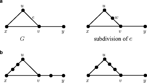

  

  (a) Subdivision of edge e of graph G, (b) two homeomorphs of graph G

Kuratowski’s theorem [129] characterizing planar graphs was one of the major breakthrough results in graph theory of the 20th century. As mentioned earlier, while examining planarity of graphs, we need only consider simple graphs since the presence of loops and multiple edges does not affect the planarity of graphs. Consequently, a graph is planar if and only if its underlying simple graph is planar. We therefore consider in this section only (finite) simple graphs. We recall that for any edge e of a graph G, G − e is the subgraph of G obtained by deleting the edge e, whereas G ∘ e denotes the contraction of e. We always discard isolated vertices when edges get deleted and remove the new multiple edges when edges get contracted. More generally, for a subgraph H of G, G ∘ H denotes the graph obtained by the successive contractions of all the edges of H in G. The resulting graph is independent of the order of contraction. Moreover, if G is planar, then G ∘ e is planar; consequently, G ∘ H is planar. In other words, if G ∘ H is nonplanar for some subgraph H of G, then G is also nonplanar. Moreover, any two homeomorphic graphs are contractible to the same graph.

Definition 8.7.2.

If G ∘ H = K, we call K a contraction of G; we also say that G is contractible to K. G is said to be subcontractible to K if G has a subgraph H contractible to K. We also refer to this fact by saying that K is a subcontraction of G. 

Example 8.7.3.

For instance, in Fig. 8.16, graph G is subcontractible to the triangle abc. (Take H to be the cycle abcd and contract the edge ad in H. By abuse of notation, the new vertex is denoted by a or d. ) We note further that if G′ is a homeomorph of G, then contraction of one of the edges incident at each vertex of degree 2 in V (G′) ∖ V (G) results in a graph homeomorphic to G.

Fig. 8.16

Graph G subcontractible to triangle abc

Our first aim is to prove the following result, which was established by Wagner [186] and, independently, by Harary and Tutte [96].

Theorem 8.7.4 ([96,  186]). 

A graph is planar if and only if it is not subcontractible to K ₅ or K _3,3.

As a consequence, we establish Kuratowski’s characterization theorem for planar graphs.

Theorem 8.7.5 (Kuratowski [129]). 

A graph is planar if and only if it has no subgraph homeomorphic to K ₅ or K _3,3.

The proofs of Theorems 8.7.4 and 8.7.5, as presented here, are due to Fournier [68]. Recall that any subgraph and any contraction of a planar graph are both planar.

Definition 8.7.6.

A simple connected nonplanar graph G is irreducible if, for each edge e of G, G ∘ e is planar.

For instance, both K ₅ and K _3, 3 are irreducible.

Proof of theorem 4.

If G has a subgraph G ₀ contractible to K ₅ or K _3, 3, then, since K ₅ and K _3, 3 are nonplanar, G ₀ and therefore G are nonplanar.

We now prove the converse. Assume that G is a simple connected nonplanar graph. By Theorem 8.2.8, at least one block of G is nonplanar. Hence, assume that G is a simple 2-connected nonplanar graph. We now show that G has a subgraph contractible to K ₅ or K _3, 3. 

Keep contracting edges of G (and delete the new multiple edges, if any, at each stage of the contraction) until a (2-connected) irreducible (nonplanar) graph H results. Clearly, δ(H) ≥ 3. Now, if e and f are any two distinct edges of G, then (G ∘ e) − f = (G − f) ∘ e. Hence, the graph H may as well be obtained by deleting a set (which may be empty) of edges of G, resulting in a subgraph G ₀ of G and then contracting a subgraph of G ₀. We now complete the proof of the theorem by showing that H has a subgraph K homeomorphic (and hence contractible) to K ₅ or K _3, 3. In this case, G has the subgraph G ₀, which is contractible to K ₅ or K _3, 3. 

Let e = ab ∈ E(H) and H′ = H − { a, b}. Then H′ is connected. If not, {a, b} is a vertex cut of H. Let ${G}_{1}^{{\prime}},\ldots ,{G}_{r}^{{\prime}}$ be the components of H′. As H is irreducible, $H - V ({G}_{r}^{{\prime}})$ is planar, and there exists a plane embedding of H′ in which the edge ab is in the exterior face. As ${G}_{r}^{{\prime}}$ is planar, ${G}_{r}^{{\prime}}$ can be embedded in this exterior face of H′. This would make H a planar graph, a contradiction. Thus, H′ is connected.]

Case 1.

H′ has a cut vertex v. Let G ₁, G ₂, …, G _r  (r ≥ 2) be the components of H′ − { v}, and let G ₁, G ₂, …, G _s , 0 ≤ s ≤ r, be those components that are connected to both a and b. (see Fig. 8.17). If r > s, then each of G _s + 1, …, G _r is connected to only one of a or b. Assume that G _r is connected to b and not to a. From the plane representation of G ∘ (G _s + 1 ∪… ∪G _r ), the contraction of G obtained by contracting the edges of G _s + 1, …, G _r , we can obtain a plane representation of H′ (see Fig. 8.17). [In fact, if G _r is contracted to the vertex w _r , then as the subgraph A _r  = 〈v, b, v(G _r )〉 of H′ is planar, the pair of edges {vw _r , w _r b} can be replaced by the planar subgraph A _r and so on.] Hence, this case cannot arise. Consequently, r = s. If r = s = 2, the plane embeddings of H′ ∘ G ₁ and H′ ∘ G ₂ yield a plane embedding of H′, a contradiction (see Fig. 8.18). Consequently, r = s  ≥ 3. In this case, H′ contains a homeomorph of K _3, 3 (see Fig. 8.19), with {w ₁, w ₂, w ₃ ; a, b, v} being the vertex set of K _3, 3. (Other possibilities for w ₁, w ₂, w ₃ will also yield a homeomorph of K _3, 3. )

Fig. 8.17

Graph H for case 1 of proof of Theorem 8.7.4

Fig. 8.18

Plane embedding for case 1 of proof of Theorem 8.7.4

Fig. 8.19

Homeomorph for case 1 of proof of Theorem 8.7.4

Case 2.

H′ is 2-connected. Then H′ contains a cycle C of length at least 3. Consider a plane embedding of H ∘ e (where e = ab, as above). If c denotes the new vertex to which a and b get contracted, (H ∘ e) − c = H′. We may therefore suppose without loss of generality that c is in the interior of the cycle C in the plane embedding of H ∘ e. 

Now, the edges of H ∘ e incident to c arise out of edges of H incident to a or b. There arise three possibilities with reference to the positions of the edges of H ∘ e incident to c relative to the cycle C. 

• (i) Suppose the edges incident to c occur so that the edges incident to a and the edges incident to b in H are consecutive around c in a plane embedding of H ∘ e, as shown in Fig. 8.20a. Since H is a minimal nonplanar graph, the paths from c to C can only be single edges. Then the plane representation of H ∘ e gives a plane representation of H, as in Fig. 8.20b, a contradiction. So this possibility cannot arise.

  Fig. 8.20

  

  First configuration for case 2 of proof of Theorem 8.7.4. Edges incident to a and b are marked a and b, respectively

  Fig. 8.21

  

  Second configuration for case 2 of proof of Theorem 8.7.4. Edges incident to both a and b are marked ab

• (ii) Suppose there are three edges of H ∘ e incident with c, with each edge corresponding to a pair of edges of H, one incident to a and the other to b, as in Fig. 8.21a. Then H contains a subgraph contractible to K ₅, as shown in Fig. 8.21b.

  We are now left with only one more possibility.

• (iii) There are four edges of H ∘ e incident to c, and they arise alternately out of edges incident to a and b in H, as in Fig. 8.22a. Then there arises in H a homeomorph of K _3, 3, as shown in Fig. 8.22b. The sets X = { a, t ₂, t ₄} and Y = { b, t ₁, t ₃} are the sets of the bipartition of this homeomorph of K _3, 3.

Fig. 8.22

Third configuration for case 2 of proof of Theorem 8.7.4

We now proceed to prove Theorem 8.7.5.

Proof of theorem 5.

The “sufficiency” part of the proof is trivial. If G contains a homeomorph of either K ₅ or K _3, 3, G is certainly nonplanar, since a homeomorph of a planar graph is planar.

Assume that G is connected and nonplanar. Remove edges from G one after another until we get an edge-minimal connected nonplanar subgraph G ₀ of G; that is, G ₀ is nonplanar and for any edge e of G, G ₀ − e is planar. Now contract the edges in G ₀ incident with vertices of degree at most 2 in some order. Let us denote the resulting graph by ${G}_{0}^{{\prime}}.$ Then ${G}_{0}^{{\prime}}$ is nonplanar, whereas ${G}_{0}^{{\prime}}- e$ is planar for any edge e of ${G}_{0}^{{\prime}},$ and the minimum degree of ${G}_{0}^{{\prime}}$ is at least 3. We now have to show that ${G}_{0}^{{\prime}}$ contains a homeomorph of K ₅ or K _3, 3. 

By Theorem 8.7.4, ${G}_{0}^{{\prime}}$ is subcontractible to K ₅ or K _3, 3. This means that ${G}_{0}^{{\prime}}$ contains a subgraph H that is contractible to K ₅ or K _3, 3. As ${G}_{0}^{{\prime}}- e$ is planar for any edge e of ${G}_{0}^{{\prime}},$ ${G}_{0}^{{\prime}} = H.$ Thus, ${G}_{0}^{{\prime}}$ itself is contractible to K ₅ or K _3, 3. If ${G}_{0}^{{\prime}}$ is either K ₅ or K _3, 3, we are done. Assume now that ${G}_{0}^{{\prime}}$ is neither K ₅ nor K _3, 3. Let e ₁, e ₂, …, e _r be the edges of ${G}_{0}^{{\prime}},$ when contracted in order, that result in a K ₅ or K _3, 3. 

First, let us assume that r = 1, so that ${G}_{0}^{{\prime}}\circ {e}_{1}$ is either K ₅ or K _3, 3. Suppose that ${G}_{0}^{{\prime}}\circ {e}_{1} = {K}_{3,3}$ with {x ₁, x ₂, x ₃} and {y ₁, y ₂, y ₃} as the partite sets of vertices. Suppose that x ₁ is the vertex obtained by identifying the ends of e ₁. We may then take e ₁ = x ₁ a (by abuse of notation), where a is a vertex distinct from the x _i ’s and y _j ’s (Fig. 8.23a). If a is adjacent to all of y ₁, y ₂ and y ₃, then {a, x ₂, x ₃} and {y ₁, y ₂, y ₃} form a bipartition of a K _3, 3 in ${G}_{0}^{{\prime}}.$ If a is adjacent to only one or two of {y ₁, y ₂, y ₃} (Fig. 8.23b), then again ${G}_{0}^{{\prime}}$ contains a homeomorph of K _3, 3. 

Fig. 8.23

Graphs for proof of Theorem 8.7.5

Next, let us assume that ${G}_{0}^{{\prime}}\circ {e}_{1} = {K}_{5}$ with vertex set {v ₁, v ₂, v ₃, v ₄, v ₅}. Suppose that v ₁ is the vertex obtained by identifying the ends of e ₁. As before, we may take e ₁ = v ₁ a, where a∉{v ₁, v ₂, v ₃, v ₄, v ₅}. If a is adjacent to all of {v ₂, v ₃, v ₄, v ₅}, then ${G}_{0}^{{\prime}}- {v}_{1}$ is a K ₅, contradiction to the fact that any proper subgraph of ${G}_{0}^{{\prime}}$ is planar. If a is adjacent to only three of {v ₂, v ₃, v ₄, v ₅}, say v ₂, v ₃, and v ₄, then the edge-induced subgraph of ${G}_{0}^{{\prime}}$ induced by the edges av ₁, av ₂, av ₃, av ₄, v ₁ v ₅, v ₂ v ₃, v ₂ v ₄, v ₂ v ₅, v ₃ v ₄, v ₃ v ₅, and v ₄ v ₅ is a homeomorph of K ₅. In this case, ${G}_{0}^{{\prime}}$ also contains a homeomorph of K _3, 3. Since ${d}_{{G}_{0}^{{\prime}}}({v}_{1}) \geq 3,$ v ₁ is adjacent to at least one of v ₂, v ₃, and v ₄, say v ₂. Then the edge-induced subgraph of ${G}_{0}^{{\prime}}$ induced by the edges in {av ₁, av ₃, av ₄, v ₁ v ₂, v ₂ v ₃, v ₂ v ₄, v ₁ v ₅, v ₃ v ₅, v ₄ v ₅} is a K _3, 3, with {a, v ₄, v ₅} and {v ₁, v ₂, v ₃} forming the bipartition. We now consider the case when a is adjacent to only two of v ₂, v ₃, v ₄ and v ₅, say v ₂ and v ₃. Then, necessarily, v ₁ is adjacent to v ₄ and v ₅ (since on contraction of the edge v ₁ a, v ₁ is adjacent to v ₂, v ₃, v ₄, and v ₅). In this case ${G}_{0}^{{\prime}}$ also contains a K _3, 3 (see Fig. 8.24). Finally, the case when a is adjacent to at most one of v ₂, v ₃, v ₄, and v ₅ cannot arise since the degree of a is at least 3 in ${G}_{0}^{{\prime}}.$ Thus, in any case, we have proved that when r = 1, ${G}_{0}^{{\prime}}$ contains a homeomorph of K _3, 3. The result can now easily be seen to be true by induction on r. Indeed, if H ₂ = H ₁ ∘ e and H ₂ contains a homeomorph of K _3, 3, then H ₁ contains a homeomorph of K _3, 3.

The nonplanarity of the Petersen graph (Fig. 8.25a) can be established by showing that it is contractible to K ₅ (see Fig. 8.25b) or by showing that it contains a homeomorph of K _3, 3 (see Fig. 8.25c).

Fig. 8.24

Fig. 8.25

Nonplanarity of the Petersen graph. (a) The Petersen graph P, (b) contraction of P to K ₅, (c) A subdivision of K _3, 3 in P

Exercise 7.1.

Prove that the following graph is nonplanar.

8.8 Hamiltonian Plane Graphs

An elegant necessary condition for a plane graph to be Hamiltonian was given by Grinberg [78].

Theorem 8.8.1.

Let G be a loopless plane graph having a Hamilton cycle C. Then ${\sum \nolimits }_{i=2}^{n}(i - 2)({\phi }_{i}^{{\prime}}- {\phi^\prime}_{i}^{{\prime}}) = 0,$ where ${\phi }_{i}^{{\prime}}$ and ${\phi }_{i}^{{\prime\prime}}$ are the numbers of faces of G of degree i contained in int C and ext C, respectively.

Proof.

Let E′ and E′ denote the sets of edges of G contained in int C and ext C, respectively, and let | E′ |  = m′ and | E′ |  = m′. Then int C contains exactly m′ + 1 faces (see Fig. 8.26), and so

$$\sum \limits_{i=2}^{n}{\phi }_{ i}^{{\prime}} = m^\prime + 1.$$

(8.1)

(Since G is loopless, ${\phi }_{1}^{{\prime}} = {\phi }_{1}^{{\prime\prime}} = 0.$)

Fig. 8.26

Graph for proof of Theorem 8.8.1

Moreover, each edge in int C is on the boundary of exactly two faces in int C, and each edge of C is on the boundary of exactly one face in int C. Hence, counting the edges of all the faces in int C, we get

$$\sum \limits_{i=2}^{n}i{\phi }_{ i}^{{\prime}} = 2m^\prime + n.$$

(8.2)

Eliminating m′ from (8.1) and (8.2), we get

$$\sum \limits_{i=2}^{n}(i - 2){\phi }_{ i}^{{\prime}} = n - 2.$$

(8.3)

Similarly,

$$\sum \limits_{i=2}^{n}(i - 2){\phi^\prime}_{ i}^{{\prime}} = n - 2.$$

(8.4)

Equations (8.3) and (8.4) give the required result.

Grinberg’s condition is quite useful in that by applying this result, many plane graphs can easily be shown to be non-Hamiltonian by establishing that they do not satisfy the condition.

Example 8.8.2.

The Herschel graph G of Fig. 5.4 is non-Hamiltonian.

Proof.

G has nine faces and all the faces are of degree 4. Hence, if G were Hamiltonian, we must have $2({\phi }_{4}^{{\prime}}- {\phi }_{4}^{{\prime\prime}}) = 0.$ This means that ${\phi }_{4}^{{\prime}} = {\phi }_{4}^{{\prime\prime}}.$ This is impossible, since ${\phi }_{4}^{{\prime}} + {\phi }_{4}^{{\prime\prime}}\, =$ (number of faces of degree 4 in G) = 9 is odd. Hence, G is non-Hamiltonian. (In fact, it is the smallest planar non-Hamiltonian 3-connected graph.)

Exercise 8.1.

Does there exist a plane Hamiltonian graph with faces of degrees 5, 7, and 8, and with just one face of degree 7?

Exercise 8.2.

Prove that the Grinberg graph given in Fig. 8.27 is non-Hamiltonian.

Fig. 8.27

The Grinberg graph

8.9 Tait Coloring

In an attempt to solve the four-color problem, Tait considered edge colorings of 2-edge-connected cubic planar graphs. He conjectured that every such graph was 3-edge colorable. Indeed, he could prove that his conjecture was equivalent to the four-color problem (see Theorem 8.9.1). Tait did this in 1880. He even went to the extent of giving a “proof” of the four-color theorem using this result. Unfortunately, Tait’s proof was based on the wrong assumption that any 2-edge-connected cubic planar graph is Hamiltonian. A counterexample to his assumption was given by Tutte in 1946 (65 years later). The graph given by Tutte is the graph of Fig. 8.28. It is a non-Hamiltonian cubic 3-connected (and therefore 3-edge-connected; see Theorem 3.3.4) planar graph. Tutte used ad hoc techniques to prove this result. (The Grinberg condition does not establish this result.)

Fig. 8.28

The Tutte graph

We indicate below the proof of the fact that the Tutte graph of Fig. 8.28 is non-Hamiltonian. The graphs G ₁ to G ₅ mentioned below are shown in Fig. 8.29.

Fig. 8.29

Graphs G ₁ to G ₅

It is easy to check that there is no Hamilton cycle in the graph G ₁ containing both of the edges e ₁ and e ₂. Now, if there is a Hamilton cycle in G ₂ containing both of the edges ${e}_{1}^{{\prime}}$ and ${e}_{2}^{{\prime}},$ then there will be a Hamilton cycle in G ₁ containing e ₁ and e ₂. Hence, there is no Hamilton cycle in G ₂ containing ${e}_{1}^{{\prime}}$ and ${e}_{2}^{{\prime}}.$ In G ₃ − e′, u and w are vertices of degree 2. Hence, if G ₃ − e′ were Hamiltonian, then in any Hamilton cycle of G ₃ − e′, both the edges incident to u as well as both the edges incident to w must be consecutive. This would imply that G ₂ has a Hamilton cycle containing ${e}_{1}^{{\prime}}$ and ${e}_{2}^{{\prime}},$ which is not the case. Consequently, any Hamilton cycle of G ₃ must contain the edge e′. It follows that there exists no Hamilton path from x to y in G ₃ − w. A redrawing of G ₃ − w is the graph G ₄. It is called the “Tutte triangle.” The Tutte graph (Fig. 8.28) contains three copies of G ₄ together with a vertex v ₀. It has been redrawn as graph G ₅ of Fig. 8.29. Suppose G ₅ is Hamiltonian with a Hamilton cycle C. If we describe C starting from v ₀, it is clear that C must visit each copy of G ₄ exactly once. Hence, if C enters a copy of G ₄, it must exit that copy through x or y after visiting all the other vertices of that copy. But this means that there exists a Hamilton path from y to x (or from x to y) in G ₄, a contradiction. Thus, the Tutte graph G ₅ is non-Hamiltonian.

We now give the proof of Tait’s result. Recall that by Vizing–Gupta’s theorem (Theorem 7.5.5), every simple cubic graph has chromatic index 3 or 4. A 3-edge coloring of a cubic planar graph is often called a Tait coloring.

Theorem 8.9.1.

The following statements are equivalent:

• (i) All plane graphs are 4-vertex-colorable.

• (ii) All plane graphs are 4-face-colorable.

• (iii) All simple 2-edge-connected cubic planar graphs are 3-edge-colorable (i.e., Tait colorable).

Proof.

• (i) ⇒ (ii). Let G be a plane graph. Let G ^∗ be the dual of G (see Sect. 8.4). Then, since G ^∗ is a plane graph, it is 4-vertex-colorable. If v ^∗ is a vertex of G ^∗, and f _v is the face of G corresponding to v ^∗, assign to f _v the color of v ^∗ in a 4-vertex coloring of G ^∗. Then, by the definition of G ^∗, it is clear that adjacent faces of G will receive distinct colors. (See Fig. 8.30, in which f _v and f _w receive the colors of v ^∗ and w ^∗, respectively.) Thus, G is 4-face-colorable.

  Fig. 8.30

  

  Graph for proof of (i) ⇒ (ii) in Theorem 8.9.1

• (ii) ⇒ (iii). Let G be a plane embedding of a 2-edge-connected cubic planar graph. By assumption, G is 4-face-colorable. Denote the four colors by (0, 0), (1, 0), (0, 1), and (1, 1), the elements of the ring ${\mathbb{Z}}_{2} \times {\mathbb{Z}}_{2}.$ If e is an edge of G that separates the faces, say f ₁ and f ₂, color e with the color given by the sum (in ${\mathbb{Z}}_{2} \times {\mathbb{Z}}_{2}$) of the colors of f ₁ and f ₂. Since G has no cut edge, each edge is the common boundary of exactly two faces of G. This gives a 3-edge coloring of G using the colors (1, 0), (0, 1), and (1, 1), since the sum of any two distinct elements of ${\mathbb{Z}}_{2} \times {\mathbb{Z}}_{2}$ is not (0, 0) (see Fig. 8.31).

  Fig. 8.31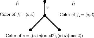

  

  Graph for proof of (ii) ⇒ (iii) in Theorem 8.9.1

• (iii) ⇒ (i) Let G be a planar graph. We want to show that G is 4-vertex-colorable. We may assume without loss of generality that G is simple. Let $\tilde{G}$ be a plane embedding of G. Then $\tilde{G}$ is a spanning subgraph of a plane triangulation T, (see Sect. 8.2), and hence it suffices to prove that T is 4-vertex-colorable.

Let T ^∗ be the dual of T. Then T ^∗ is a 2-edge-connected cubic plane graph. By our assumption, T ^∗ is 3-edge-colorable using, for example, the colors c ₁, c ₂, and c ₃. Since T ^∗ is cubic, each of the above three colors is represented at each vertex of T ^∗. Let ${T}_{ij}^{{_\ast}}$ be the edge subgraph of T ^∗ induced by the edges of T ^∗ which have been colored using the colors c _i and c _j . Then ${T}_{ij}^{{_\ast}}$ is a disjoint union of even cycles, and thus it is 2-face-colorable. But each face of T ^∗ is the intersection of a face of ${T}_{12}^{{_\ast}}$ and a face of ${T}_{23}^{{_\ast}}$ (see Fig. 8.32). Now the 2-face colorings of ${T}_{12}^{{_\ast}}$ and ${T}_{23}^{{_\ast}}$ induce a 4-face coloring of T ^∗ if we assign to each face of T ^∗ the (unordered) pair of colors assigned to the faces whose intersection is f. Since ${T}^{{_\ast}} = {T}_{12}^{{_\ast}}\cup {T}_{23}^{{_\ast}},$ this defines a proper 4-face coloring of T ^∗. Thus, $\chi (G) = \chi (\tilde{G}) \leq \chi (T) = {\chi }^{{_\ast}}({T}^{{_\ast}}) \leq 4,$ and G is 4-vertex-colorable. (Recall that χ^∗(T ^∗) is the face-chromatic number of T ^∗. )

Exercise 9.1.

Exhibit a 3-edge coloring for the Tutte graph (see Fig. 8.28).

8.10 Notes

The proof of Heawood’s theorem uses arguments based on paths in which the vertices are colored alternately by two colors. Such paths are called “Kempe chains” after Kempe [121], who first used such chains in his “proof” of the 4CC. Even though Kempe’s proof went wrong, his idea of using Kempe chains and switching the colors in such chains had been effectively exploited by Heawood [103] in proving his five-color theorem (Theorem 8.6.2) for planar graphs, as well as by Appel, Haken, and Koch [8] in settling the 4CC. As the reader might notice, the same technique had been employed in the proof of Brooks’ theorem (Theorem 7.3.7). Chronologically, Francis Guthrie conceived the four-color theorem in 1852 (if not earlier). Kempe’s purported “proof” of the 4CC was given in 1879, and the mistake in his proof was pointed out by Heawood in 1890. The Appel–Haken–Koch proof of the 4CC was first announced in 1976. Between 1879 and 1976, graph theory witnessed an unprecedented growth along with the methods to tackle the 4CC. The reader who is interested in getting a detailed account of the four-color problem may consult Ore [152] and Kainen and Saaty [120].

Fig. 8.32

Graph for proof of (iii) ⇒ (i) for Theorem 8.9.1

Even though the Tutte graph of Fig. 8.28 shows that not every cubic 3-connected planar graph is Hamiltonian, Tutte himself showed that every 4-connected planar graph is Hamiltonian [180].

References

Adiga, C., Balakrishnan, R., So, W.: The skew energy of a digraph. Linear Algebra Appl. 432, 1825–1835 (2010)
Aharoni, R., Szabó, T.: Vizing’s conjecture for chordal graphs. Discrete Math. 309(6), 1766–1768 (2009)
Aho, A.V., Hopcroft, J.E., Ullman, J.D.: The Design and Analysis of Computer Algorithms. Addison-Wesley, Reading, MA (1974)
Akbari, S., Moazami, F., Zare, S.: Kneser graphs and their complements are hyperenergetic. MATCH Commun. Math. Comput. Chem. 61, 361–368 (2009)
Apostol, T.M.: Introduction to Analytic Number Theory. Springer-Verlag, Berlin (1989)
Appel, K., Haken, W.: Every planar map is four colorable: Part I-discharging. Illinois J. Math. 21, 429–490 (1977)
Appel, K., Haken, W.: The solution of the four-color-map problem, Sci. Amer. 237(4) 108–121 (1977)
Appel, K., Haken, W., Koch, J.: Every planar map is four colorable: Part II—reducibility. Illinois J. Math. 21, 491–567 (1977)
Aravamudhan, R., Rajendran, B.: Personal communication
Balakrishnan, R.: The energy of a graph. Linear Algebra Appl. 387, 287–295 (2004)
Balakrishnan, R., Paulraja, P.: Powers of chordal graphs. J. Austral. Math. Soc. Ser. A 35, 211–217 (1983)
Balakrishnan, R., Paulraja, P.: Chordal graphs and some of their derived graphs. Congressus Numerantium 53, 71–74 (1986)
Balakrishnan, R., Kavaskar, T., So, W.: The energy of the Mycielskian of a regular graph. Australasian J. Combin. 52, 163–171 (2012)
Bapat, R.B.: Graphs and Matrices, Universitext Series, Springer. (2011)
Barcalkin, A.M., German, L.F.: The external stability number of the Cartesian product of graphs. Bul. Akad. Štiince RSS Moldoven 94(1), 5–8 (1979)
Behzad, M., Chartrand, G., Lesniak-Foster, L.: Graphs and Digraphs. Prindle, Weber & Schmidt International Series, Boston, MA (1979)
Beineke, L.W.: On derived graphs and digraphs. In: Sachs, H., Voss, H.J., Walther, H. (eds.) Beiträge zur Graphentheorie, pp. 17–33. Teubner, Leipzig (1968)
Benzer, S.: On the topology of the genetic fine structure. Proc. Nat. Acad. Sci. USA 45, 1607–1620 (1959)
Berge, C.: Graphs and Hypergraphs, North-Holland Mathematical Library, Elsevier, 6, (1973)
Berge, C.: Graphes, Third Edition. Dunod, Paris, 1983 (English, Second and revised edition of part 1 of the 1973 English version, North-Holland, 1985)
Berge, C., Chvátal, V.: Topics on perfect graphs. Annals of Discrete Mathematics, 21. North Holland, Amsterdam (1984)
Biggs, N.: Algebraic Graph Theory, 2nd ed. Cambridge University Press, Cambridge (1993)
Birkhoff, G., Lewis, D.: Chromatic polynomials. Trans. Amer. Math. Soc. 60, 355–451 (1946)
Bondy, J.A.: Pancyclic graphs. J. Combin. Theory Ser. B 11, 80–84 (1971)
Bondy, J.A., Chvátal, V.: A method in graph theory. Discrete Math. 15, 111–135 (1976)
Bondy, J.A., Halberstam, F.Y.: Parity theorems for paths and cycles in graphs. J. Graph Theory 10, 107–115 (1986)
Bondy, J.A., Murty, U.S.R.: Graph Theory with Applications. MacMillan, India (1976)
Bollobás, B.: Modern Graph Theory, Graduate Texts in Mathematics. Springer (1998)
Brešar, B., Rall, D.F.: Fair reception and Vizing’s conjecture. J. Graph Theory 61(1), 45–54 (2009)
Brešsar, B., Dorbec, P., Goddard, W., Hartnell, B.L., Henning, M.A., Klavžar, S., Rall, D.F.: Vizing’s conjecture: A survey and recent results. J. Graph Theory, 69, 46–76 (2012)
Brooks, R.L.: On coloring the nodes of a network. Proc. Cambridge Philos. Soc. 37, 194–197 (1941)
Bryant, D.: Another quick proof that K 10≠P + P + P. Bull. ICA Appl. 34, 86 (2002)
Cayley, A.: On the theory of analytical forms called trees. Philos. Mag. 13, 172–176 (1857); Mathematical Papers, Cambridge 3, 242–246 (1891)
Chartrand, G., Ollermann, O.R.: Applied and algorithmic graph theory. International Series in Pure and Applied Mathematics. McGraw-Hill, New York (1993)
Chartrand, G., Wall, C.E.: On the Hamiltonian index of a graph. Studia Sci. Math. Hungar. 8, 43–48 (1973)
Chudnovsky, M., Robertson, N., Seymour, P., Thomas, R.: The strong perfect graph theorem. Ann. Math. 164, 51–229 (2006)
Chung, F.R.K.: Diameters and eigenvalues. J. Amer. Math. Soc. 2, 187–196 (1989)
Chvátal, V.: On Hamilton’s ideals. J. Combin. Theory Ser. B 12, 163–168 (1972)
Chvátal, V., Erdős, P.: A note on Hamiltonian circuits. Discrete Math. 2, 111–113 (1972)
Chvátal, V., Sbihi, N.: Bull-free Berge graphs are perfect. Graphs Combin. 3, 127–139 (1987)
Clark, J., Holton, D.A.: A First Look at Graph Theory. World Scientific, Teaneck, NJ (1991)
Clark, W.E., Suen, S.: An inequality related to Vizings conjecture. Electron. J. Combin. 7(1), Note 4, (electronic) (2000)
Clark, W.E., Ismail, M.E.H., Suen, S.: Application of upper and lower bounds for the domination number to Vizing’s conjecture. Ars Combin. 69, 97–108 (2003)
Cockayne, E.J.: Domination of undirected graphs—a survey, In: Alavi, Y., Lick, D.R. (eds.) Theory and Application of Graphs in America’s Bicentennial Year. Springer-Verlag, New York (1978)
Cockayne, E.J., Hedetniemi, S.T., Miller, D.J.: Properties of hereditary hypergraphs and middle graphs. Networks 7, 247–261 (1977)
Cvetković, D.M.: Graphs and their spectra. Thesis, Univ. Beograd Publ. Elektrotehn. Fak., Ser. Mat. Fiz., No. 354–356, pp. 01–50 (1971)
Cvetković, D.M., Doob, M., Sachs, H.: Spectra of Graphs—Theory and Application, Third revised and enlarged edition. Johann Ambrosius Barth Verlag, Heidelberg/Leipzig (1995)
Deligne, P.: La conjecture de Weil I. Publ. Math. IHES 43, 273–307 (1974)
Demoucron, G., Malgrange, Y., Pertuiset, R.: Graphes planaires: Reconnaissance et construction de représentaitons planaires topologiques. Rev. Française Recherche Opérationnelle 8, 33–47 (1964)
Descartes, B.: Solution to advanced problem no. 4526. Am. Math. Mon. 61, 269–271 (1954)
Diestel, R.: Graph theory. In: Graduate Texts in Mathematics, vol. 173, 4th edn. Springer, Heidelberg (2010)
Dijkstra, E.W.: A note on two problems in connexion with graphs. Numerische Math. 1, 269–271 (1959)
Dirac, G.A.: A property of 4-chromatic graphs and some remarks on critical graphs. J. London Math. Soc. 27, 85–92 (1952)
Dirac, G.A.: Some theorems on abstract graphs. Proc. London Math. Soc. 2, 69–81 (1952)
Dirac, G.A.: Généralisations du théoréme de Menger. C.R. Acad. Sci. Paris 250, 4252–4253 (1960)
Dirac, G.A.: On rigid circuit graphs-cut sets-coloring. Abh. Math. Sem. Univ. Hamburg 25, 71–76 (1961)
Drinfeld, V.: The proof of Peterson’s conjecture for GL(2) over a global field of characteristic p. Funct. Anal. Appl. 22, 28–43 (1988)
Droll, A.: A classification of Ramanujan Cayley graphs. Electron. J. Cominator. 17, #N29 (2010)
El-Zahar, M., Pareek, C.M.: Domination number of products of graphs. Ars Combin. 31 (1991) 223–227
Fáry, I.: On straight line representation of planar graphs. Acta Sci. Math. Szeged 11, 229–233 (1948)
Ferrar, W.L.: A Text-Book of Determinants, Matrices and Algebraic Forms. Oxford University Press (1953)
Fiorini, S., Wilson, R.J.: Edge-colourings of graphs. Research Notes in Mathematics, vol. 16. Pitman, London (1971)
Fleischner, H.: Elementary proofs of (relatively) recent characterizations of Eulerian graphs. Discrete Appl. Math. 24, 115–119 (1989)
Fleischner, H.: Eulerian graphs and realted topics. Ann. Disc. Math. 45 (1990)
Ford, L.R. Jr., Fulkerson, D.R.: Maximal flow through a network. Canad. J. Math. 8, 399–404 (1956)
Ford, L.R. Jr., Fulkerson, D.R.: Flows in Networks. Princeton University Press, Princeton (1962)
Fournier, J.-C.: Colorations des arétes d’un graphe. Cahiers du CERO 15, 311–314 (1973)
Fournier, J.-C.: Demonstration simple du theoreme de Kuratowski et de sa forme duale. Discrete Math. 31, 329–332 (1980)
Fulkerson, D.R.: Blocking and anti-blocking pairs of polyhedra. Math. Programming 1, 168–194 (1971)
Fulkerson, D.R., Gross, O.A.: Incidence matrices and interval graphs. Pacific J. Math. 15, 835–855 (1965)
Garey, M.R., Johnson, D.S.: Computers and Intractability: A Guide to the Theory of NP-Completeness, W.H. Freeman & Co., San Francisco (1979)
Gibbons, A.: Algorithmic Graph Theory. Cambridge University Press, Cambridge (1985)
Gilmore, P.C., Hoffman, A.J.: A characterization of comparability graphs and interval graphs. Canad. J. Math. 16, 539–548 (1964)
Goddard, W.D., Kubicki, G., Ollermann, O.R., Tian, S.L.: On multipartite tournaments. J. Combin. Theory Ser. B 52, 284–300 (1991)
Godsil, C.D., Royle, G.: Algebraic graph theory. Graduate Texts in Mathematics, vol. 207. Springer-Verlag, Berlin (2001)
Golumbic, M.C.: Algorithmic Graph Theory and Perfect Graphs. Academic Press, New York (1980)
Gould, R.J.: Graph Theory. Benjamin/Cummings Publishing Company, Menlo Park, CA (1988)
Grinberg, É.Ja.: Plane homogeneous graphs of degree three without Hamiltonian circuits (Russian). Latvian Math. Yearbook 4, 51–58 (1968)
Gross, J.L., Tucker, T.W.: Topological Graph Theory. Wiley, New York (1987)
Gross, J.L., Yellen, J.: Handbook of graph theory. Discrete Mathematics and Its Applications, vol. 25. CRC Press, Boca Raton, FL (2004)
Gupta, R.P.: The chromatic index and the degree of a graph. Notices Amer. Math. Soc. 13, Abstract 66T–429 (1966)
Gutman, I.: The energy of a graph. Ber. Math. Stat. Sekt. Forschungszent. Graz. 103, 1–22 (1978)
Gutman, I.: The energy of a graph: Old and new results. In: Betten, A., Kohnert, A., Laue, R., Wassermann, A. (eds.) Algebraic Combinatorics and Applications, pp. 196–211, Springer, Berlin (2001)
Gutman, I., Polansky, O.: Mathematical Concepts in Organic Chemistry. Springer-Verlag, Berlin (1986)
Gutman, I., Zhou, B.: Laplacian energy of a graph. Linear Algebra Appl. 414, 29–37 (2006)
Gutman, I., Soldatović, T., Vidović, D.: The energy of a graph and its size dependence. A Monte Carlo approach. Chem. Phys. Lett. 297, 428–432 (1998)
Gutman, I., Firoozabadi, S.Z., de la Pẽna, J.A., Rada, J.: On the energy of regular graphs. MATCH Commun. Math. Comput. Chem. 57, 435–442 (2007)
Gyárfás, A., Lehel, J., Nešetril, J., Rödl, V., Schelp, R.H., Tuza, Z.: Local k-colorings of graphs and hypergraphs. J. Combin. Theory Ser. B 43, 127–139 (1987)
Hajnal, A., Surányi, J.: Über die Auflösung von Graphen in Vollständige Teilgraphen. Ann. Univ. Sci. Budapest, Eötvös Sect. Math. 1, 113–121 (1958)
Hall, P.: On representatives of subsets. J. London Math. Soc. 10, 26–30 (1935)
Hall, M. Jr.: Combinatorial Theory. Blaisdell, Waltham, MA (1967)
Harary, F.: The determinant of the adjacency matrix of a graph. SIAM Rev 4, 202–210 (1962)
Harary, F.: Graph Theory. Addison-Wesley, Reading, MA (1969)
Harary, F., Nash-Williams, C.St.J.A.: On Eulerian and Hamiltonian graphs and line graphs. Canad. Math. Bull. 8, 701–710 (1965)
Harary, F., Palmer, E.M.: Graphical Enumeration, Academic Press, New York (1973)
Harary, F., Tutte, W.T.: A dual form of Kuratowski’s theorem. Canad. Math. Bull. 8, 17–20 (1965)
Harary, F., Norman, R.Z., Cartwright, D.: Structural Models: An Introduction to the Theory of Directed Graphs. Wiley, New York (1965)
Hartnell, B., Rall, D.F.: On Vizing’s conjecture. Congr. Numer. 82, 87–96 (1991)
Hartnell, B., Rall, D.F.: Domination in Cartesian products: Vizing’s conjecture. In: Domination in Graphs, Advanced Topics, vol. 209. Monographs and Textbooks in Pure and Applied Mathematics, pp. 163–189. Marcel Dekker, New York (1998)
Haynes, T.W., Hedetniemi, S.T., Slater, P.J.: Fundamentals of Domination in Graphs. Marcel Dekker, New York (1998)
Haynes, T.W., Hedetniemi, S.T., Slater, P.J.: Domination in Graphs: Advanced Topics. Marcel Dekker, New York (1998)
Hayward, R.B.: Weakly triangulated graphs. J. Combin. Theory Ser. B 39, 200–208 (1985)
Heawood, P.J.: Map colour theorems. Quart. J. Math. 24, 332–338 (1890)
Hedetniemi, S.T.: Homomorphisms of graphs and automata. Tech. Report 03105-44-T, University of Michigan (1966)
Hell, P., Nešetril, J.: Graphs and homorphisms. Oxford Lecture Series in Mathematics and its Applications, vol. 28. Oxford University Press, Oxford (2004)
Holton, D.A., Sheehan, J.: The Petersen graph. Australian Mathematical Society Lecture Series, vol. 7, Cambridge University Press, Cambridge (1993)
Hougardy, S., Le, V.B., Wagler, A.: Wing-triangulated graphs are perfect. J. Graph Theory 24, 25–31 (1997)
Ilić, A.: The energy of unitary Cayley graphs. Linear Algebra Appl. 431, 1881–1889 (2009)
Ilić, A.: Distance spectra and distance energy of integral circulant graphs. Linear Algebra Appl. 433, 1005–1014 (2010)
Indulal, G., Gutman, I., Vijayakumar, A.: On distance energy of graphs. MATCH Commun. Math. Comput. Chem. 60, 461–472 (2008)
Irving, R.W., Manlove, D.F.: The b-chromatic number of a graph. Discrete Appl. Math. 91, 127–141 (1999)
Jacobson, M.S., Kinch, L.F.: On the domination number of product graphs: I. Ars. Combin. 18, 33–44 (1984)
Jaeger, F.: A note on sub-Eulerian graphs. J. Graph Theory 3, 91–93 (1979)
Jaeger, F.: Nowhere-zero flow problems. In: Beineke, L.W., Wilson, R.J. (eds.) Selected Topics in Graph Theory III, pp. 71–95. Academic Press, London (1988)
Jaeger, F., Payan, C.: Relations du type Nordhaus–Gaddum pour le nombre d’absorption d’un graphe simple. C. R. Acad. Sci. Paris A 274, 728–730 (1972)
Jensen, T.R., Toft, B.: Graph coloring problems. Wiley-Interscience Series in Discrete Mathematics and Optimization. Wiley, New York (1995)
Jordan, C.: Sur les assemblages de lignes. J. Reine Agnew. Math. 70, 185–190 (1869)
Jüng, H.: Zu einem Isomorphiesatz von Whitney für Graphen. Math. Ann. 164, 270–271 (1966)
Jünger, M., Pulleyblank, W.R., Reinelt, G.: On partitioning the edges of graphs into connected subgraphs. J. Graph Theory 9, 539–549 (1985)
Kainen, P.C., Saaty, T.L.: The Four-Color Problem (Assaults and Conquest). Dover Publications, New York (1977)
Kempe, A.: On the geographical problem of four colours. Amer. J. Math. 2, 193–200 (1879)
Kilpatrick, P.A.: Tutte’s first colour-cycle conjecture. Ph.D. thesis, Cape Town, (1975)
Klotz, W., Sander, T.: Some properties of unitary Cayley graphs. Electron. J. Combinator. 14, 1–12 (2007)
Koolen, J.H., Moulton, V.: Maximal energy graphs. Adv. Appl. Math. 26, 47–52 (2001)
Kouider, M., Mahéo, M.: Some bounds for the b-chromatic number of a graph. Discrete Math. 256, 267–277 (2002)
Kratochvíl, J., Tuza, Z., Voigt, M.: On the b-chromatic number of graphs. Lecture Notes Comput. Sci. 2573, 310–320 (2002)
Kruskal, J.B. Jr.: On the shortest spanning subtree of a graph and the travelling salesman problem. Proc. Amer. Math. Soc. 7, 48–50 (1956)
Kundu, S.: Bounds on the number of disjoint spanning trees. J. Combin. Theory Ser. B 17, 199–203 (1974)
Kuratowski, C.: Sur le problème des courbes gauches en topologie. Fund. Math. 15, 271–283 (1930)
Laskar, R., Shier, D.: On powers and centers of chordal graphs. Discrete Applied Math. 6, 139–147 (1983)
Lesniak, L.M.: Neighborhood unions and graphical properties. In: Alavi, Y., Chartrand, G., Ollermann, O.R., Schwenk, A.J. (eds.) Proceedings of the Sixth Quadrennial International Conference on the Theory and Applications of Graphs: Graph Theory, Combinatorics and Applications. Western Michigan University, pp. 783–800. Wiley, New York (1991)
Li, W.C.W.: Number theory with applications. Series of University Mathematics, vol. 7. World Scientific, Singapore (1996)
Li, X., Li, Y., Shi, Y.: Note on the energy of regular graphs. Linear Algebra Appl. 432, 1144–1146 (2010)
Lovász, L.: Normal hypergraphs and the perfect graph conjecture. Discrete Math. 2, 253–267 (1972)
Lovász, L.: Three short proofs in graph theory. J. Combin Theory Ser. B 19, 111–113 (1975)
Lovász, L., Plummer, M.D.: Matching theory. Annals of Discrete Mathematics, vol. 29. North-Holland Mathematical Studies, vol. 121 (1986)
Lubotzky, A., Phillips, R., Sarnak, P.: Ramanujan graphs. Combinatorica 8, 261–277 (1988)
McKee, T.A.: Recharacterizing Eulerian: Intimations of new duality. Discrete Math. 51, 237–242 (1984)
Meir, A., Moon, J.W.: Relations between packing and covering numbers of a tree. Pacific J. Math. 61, 225–233 (1975)
Menger, K.: Zur allgemeinen Kurventheorie. Fund. Math. 10, 96–115 (1927)
Moon, J.W.: On subtournaments of a tournament. Canad. Math. Bull. 9, 297–301 (1966)
Moon, J.W.: Various proofs of Cayley’s formula for counting trees. In: Harary, F. (eds.) A Seminar on Graph Theory, pp. 70–78. Holt, Rinehart and Winston, Inc., New York (1967)
Moon, J.W.: Topics on Tournaments. Holt, Rinehart and Winston Inc., New York (1968)
Mycielski, J.: Sur le coloriage des graphs. Colloq. Math. 3, 161–162 (1955)
Nash-Williams, C.St.J.A.: Edge-disjoint spanning trees of finite graphs. J. London Math. Soc. 36, 445–450 (1961)
Nebesky, L.: On the line graph of the square and the square of the line graph of a connected graph, Casopis. Pset. Mat. 98, 285–287 (1973)
Nikiforov, V.: The energy of graphs and matrices. J. Math. Anal. Appl. 326, 1472–1475 (2007)
Nordhaus, E.A., Gaddum, J.W.: On complementary graphs. Amer. Math. Monthly 63, 175–177 (1956)
Oberly, D.J., Sumner, D.P.: Every connected, locally connected nontrivial graph with no induced claw is Hamiltonian. J. Graph Theory 3, 351–356 (1979)
Ore, O.: Note on Hamilton circuits. Amer. Math. Monthly 67, 55 (1960)
Ore, O.: Theory of graphs. Amer. Math. Soc. Transl. 38, 206–212 (1962)
Ore, O.: The Four-Color Problem. Academic Press, New York (1967)
Papadimitriou, C.H., Steiglitz, K.: Combinatorial Optimization: Algorithms and Complexity. Prentice-Hall, Upper Saddle River, NJ (1982)
Parthasarathy, K.R., Ravindra, G.: The strong perfect-graph conjecture is true for K 1, 3-free graphs. J. Combin. Theory Ser. B 21, 212–223 (1976)
Parthasarathy, K.R.: Basic Graph Theory. Tata McGraw-Hill Publishing Company Limited, New Delhi (1994)
Parthasarathy, K.R., Ravindra, G.: The validity of the strong perfect-graph conjecture for (K 4 − e)-free graphs. J. Combin. Theory Ser. B 26, 98–100 (1979)
Peña, I., Rada, J.: Energy of digraphs. Linear and Multilinear Algebra 56(5), 565–579 (2008)
Petersen, J.: Die Theorie der regulären Graphen. Acta Math. 15, 193–220 (1891)
Prim, R.C.: Shortest connection networks and some generalizations. Bell System Techn. J. 36, 1389–1401 (1957)
Rall, D.F.: Total domination in categorical products of graphs. Discussiones Mathematicae Graph Theory 25, 35–44 (2005)
Ramaswamy, H.N., Veena, C.R.: On the energy of unitary Cayley graphs. Electron. J. Combinator. 16 (2009)
Ram Murty, M.: Ramanujan graphs. J. Ramanujan Math. Soc. 18(1), 1–20 (2003)
Ram Murty, M.: Ramanujan graphs and zeta functions. Jeffery-Williams Prize Lecture. Canadian Mathematical Society, Canada (2003)
Ray-Chaudhuri, D.K., Wilson, R.J.: Solution of Kirkman’s schoolgirl problem. In: Proceedings of the Symposium on Mathematics, vol. 19, pp. 187–203. American Mathematical Society, Providence, RI (1971)
Rédei, L.: Ein kombinatorischer satz. Acta. Litt. Sci. Szeged 7, 39–43 (1934)
Roberts, F.S.: Graph theory and its applications to problems in society. CBMS-NSF Regional Conference Series in Mathematics. SIAM, Philadelphia (1978)
Sachs, H.: Über teiler, faktoren und charakteristische polynome von graphen II. Wiss. Z. Techn. Hochsch. Ilmenau 13, 405–412 (1967)
Sampathkumar, E.: A characterization of trees. J. Karnatak Univ. Sci. 32, 192–193 (1987)
Schwenk, A.J., Lossers, O.P.: Solutions of advanced problems. Am. Math. Mon. 94, 885–887 (1987)
Serre, J.-P.: Trees. Springer-Verlag, New York (1980)
Shader, B., So, W.: Skew spectra of oriented graphs. Electron. J. Combinator. 16, 1–6 (2009)
Shrikhande, S.S., Bhagwandas: Duals of incomplete block designs. J. Indian Stat. Assoc. 3, 30–37 (1965)
Stevanović, D., Stanković, I.: Remarks on hyperenergetic circulant graphs. Linear Algebra Appl. 400, 345–348 (2005)
Sumner, D.P.: Graphs with 1-factors. Proc. Amer. Math. Soc. 42, 8–12 (1974)
Toida, S.: Properties of an Euler graph. J. Franklin. Inst. 295, 343–346 (1973)
Trinajstic, N.: Chemical Graph Theory—Volume I. CRC Press, Boca Raton, FL (1983)
Trinajstic, N.: Chemical Graph Theory—Volume II. CRC Press, Boca Raton, FL (1983)
Tucker, A.: The validity of perfect graph conjecture for K 4-free graphs. In: Berge, C., Chvátal, V. (eds.) Topics on Perfect Graphs, vol. 21, pp. 149–157 (1984)
Tutte, W.T.: The factorization of linear graphs. J. London Math. Soc. 22, 107–111 (1947)
Tutte, W.T.: A theorem on planar graphs. Trans. Amer. Math. Soc. 82, 570–590 (1956)
Tutte, W.T.: On the problem of decomposing a graph into n connected factors. J. London Math. Soc. 36, 221–230 (1961)
Vizing, V.G.: The Cartesian product of graphs. Vycisl/Sistemy 9, 30–43 (1963)
Vizing, V.G.: On an estimate of the chromatic class of a p-graph (in Russian). Diskret. Analiz. 3, 25–30 (1964)
Vizing, V.G.: A bound on the external stability number of a graph. Dokl. Akad. Nauk. SSSR 164, 729–731 (1965)
Vizing, V.G.: Some unsolved problems in graph theory. Uspekhhi Mat. Nauk. 23(6), 117–134 (1968)
Wagner, K.: Über eine eigenschaft der ebenen komplexe. Math. Ann. 114, 570–590 (1937)
Walikar, H.B., Acharya, B.D., Sampathkumar, E.: Recent developments in the theory of domination in graphs. MRI Lecture Notes in Mathematics, vol. 1. Mehta Research Institue, Allahabad (1979)
Walikar, H.B., Ramane, H.S., Hampiholi, P.R.: On the energy of a graph. In: Mulder, H.M., Vijayakumar, A., Balakrishnan, R. (eds.) Graph Connections, pp. 120–123. Allied Publishers, New Delhi (1999)
Walikar, H.B., Gutman, I., Hampiholi, P.R., Ramane, H.S.: Non-hyperenergetic graphs. Graph Theory Notes New York 41, 14–16 (2001)
Walikar, H.B., Ramane, H.S., Jog, S.R.: On an open problem of R. Balakrishnan and the energy of products of graphs. Graph Theory Notes New York 55, 41–44 (2008)
Welsh, D.J.A.: Matroid Theory. Academic Press, London (1976)
West, D.B.: Introduction to Graph Theory, 2nd ed. Prentice Hall, New Jersey (2001)
Whitney, H.: Congruent graphs and the connectivity of graphs. Amer. J. Math. 54, 150–168 (1932)
Yap, H.P.: Some topics in graph theory. London Mathematical Society Lecture Notes Series, vol. 108, Cambridge University Press, Cambridge (1986)
Zykov, A.A.: On some properties of linear complexes (in Russian). Math. Sbornik N. S. 24, 163–188 (1949); Amer. Math Soc. Trans. 79 (1952)
Author information
Authors and Affiliations
Rights and permissions
Copyright information
© 2012 Springer Science+Business Media New York
About this chapter
Cite this chapter
Balakrishnan, R., Ranganathan, K. (2012). Planarity. In: A Textbook of Graph Theory. Universitext. Springer, New York, NY. https://doi.org/10.1007/978-1-4614-4529-6_8
Download citation
DOI: https://doi.org/10.1007/978-1-4614-4529-6_8
Published:
Publisher Name: Springer, New York, NY
Print ISBN: 978-1-4614-4528-9
Online ISBN: 978-1-4614-4529-6
eBook Packages: Mathematics and StatisticsMathematics and Statistics (R0)