
Abstract
Section 1.1 is devoted to the study of dynamical processes in electric circuits. It includes derivations of the constitutive relations of elements of electric circuits (capacitors, inductors) and describes current and voltage sources and Kirchhoff’s law. Section 1.2 deals with dynamical processes in mechatronic systems (transducers) and the electromagnetomechanical circuit. In Sect. 1.3, the dynamics and control of a mass levitating in magnetic and gravitational fields is discussed. Two cases of numerical control are considered and verified experimentally. In Sect. 1.4, combined analytical and numerical analyses of vibrations in string-type generators is carried out. The vibrations of a string are governed by a PDE, whereas the dynamics of an amplifier is governed by an ODE with a time delay. The voltage generated on the string ends depends on both electromagnetic induction and string vibration speed. An averaged set of equations is derived and numerically studied. Finally, in Sect.1.5, a 2-DOF nonlinear dynamics of a rotor supported by a magnetohydrodynamic bearing is investigated using perturbation analysis. Two modes corresponding to the vertical and horizontal vibrations of the rotor are coupled. The non-resonant case and the various resonant cases (with and without an internal resonance) are considered. Frequency-response curves are obtained. When the amplitude of the external harmonic excitation is near one of the natural frequencies of the vibrations and the system experiencing internal resonance, a saturation phenomenon occurs.
Access provided by Autonomous University of Puebla. Download chapter PDF
Keywords
These keywords were added by machine and not by the authors. This process is experimental and the keywords may be updated as the learning algorithm improves.
Section 1.1 is devoted to the study of dynamical processes in electric circuits. It includes derivations of the constitutive relations of elements of electric circuits (capacitors, inductors) and describes current and voltage sources and Kirchhoff’s law. Section 1.2 deals with dynamical processes in mechatronic systems (transducers) and the electromagnetomechanical circuit. In Sect. 1.3, the dynamics and control of a mass levitating in magnetic and gravitational fields is discussed. Two cases of numerical control are considered and verified experimentally. In Sect. 1.4, combined analytical and numerical analyses of vibrations in string-type generators is carried out. The vibrations of a string are governed by a PDE, whereas the dynamics of an amplifier is governed by an ODE with a time delay. The voltage generated on the string ends depends on both electromagnetic induction and string vibration speed. An averaged set of equations is derived and numerically studied. Finally, in Sect. 1.5, a 2-DOF nonlinear dynamics of a rotor supported by a magnetohydrodynamic bearing is investigated using perturbation analysis. Two modes corresponding to the vertical and horizontal vibrations of the rotor are coupled. The non-resonant case and the various resonant cases (with and without an internal resonance) are considered. Frequency-response curves are obtained. When the amplitude of the external harmonic excitation is near one of the natural frequencies of the vibrations and the system experiencing internal resonance, a saturation phenomenon occurs. When the amplitude of the external excitation increases, after some critical value the energy pumping between various submotions of the rotor occurs for each mode. Further, it is shown that in the case of rigid magnetic materials, hysteresis may be a cause of chaotic vibrations of the rotor. Chaotic regions and the amplitude level contours of the rotor vibrations are obtained in various control parameter planes.
1.1 Dynamical Processes in Electric Circuits
In Sect. 1.1, to write equations of dynamics in mechatronic systems, we will make use of the unified approach developed from mechanics and based on variational calculus [1, 2]. It should be emphasized that such an approach is based on the theory of the quasistatic electromagnetic field whose changes are slow enough to neglect the interactions occurring between magnetic and electric fields. Electric circuits consist of passive elements such as resistors, coils, and capacitors and active elements such as voltage and current sources.
1.1.1 Constitutive Relations of Elements of Electric Circuits
1.1.1.1 The Capacitor
Figure 1.1a shows a schematic of a capacitor to whose plates the voltage U was applied and an example of a constitutive function U(Q) (Fig. 1.1b).

Schematic diagram of a capacitor (a) and a constitutive function U(Q) (b)
As the capacitor is charged, the charge Q is supplied to one of its plates and removed from another. The change in the charge on the plates separated by a dielectric produces the current flow
During charging, a potential difference appears between the plates of the capacitor (voltage U). An example of measurements of the voltage U and the corresponding charge Q in static conditions leads to the construction of graph U(Q) (Fig. 1.1b).
The electric energy gathered in the capacitor E e(Q) is equivalent to the work done while charging it from value 0 to Q and is equal to
where \({N}^{\mathrm{e}} =\dot{ {W}}^{\mathrm{e}}\) is the power supplied to the system, and during transformations (1.1) was used. The value of integral (1.2) corresponds to the area under the curve U(Q) in Fig. 1.1b. If in the neighborhood of the operating point A of the capacitor we conduct the linearization, we obtain
and integrating we have
A complementary state function may be easily determined on the basis of Fig. 1.1b, and it is equal to
where E c e(I) is the so-called complementary energy.
Making use of the method described earlier it is easy to notice that
1.1.1.2 The Inductor
It is widely known that if the current of intensity I flows through a conductor, then around the conductor there is generated a magnetic field proportional to the intensity of the flowing current. In turn, if the conductor is situated in the changing magnetic field, then the voltage will be generated at its ends.
If the conductor is wound in turns so as to form a coil, then the generated magnetic flux Φ is proportional to the intensity of the current I flowing through the coil. If we now put a ferromagnetic core inside the coil, then the density of the magnetic flux is substantially increased.
According to Faraday’s law of induction, the voltage induced in a conductor is equal to
If we have an ideal conductor, then I = const (intensity of the current does not change in time) and a magnetic flux Φ = const. In this case, from (1.7) it follows that U = 0 (the voltage in the conductor is not induced). If we perform the linearization of the function I(Φ) (Fig. 1.2b) in the neighborhood of operating point A, then
where L is called the inductance.

Schematic diagram of an inductor (a) and the graph of the constitutive function (b)
As in the case of the capacitor, the magnetic energy stored in an ideal conductor is calculated based on the knowledge of the power supplied to the conductor (to the electric circuit) N e = UI, and it is equal to
On the basis of the method described earlier we calculate the magnetic energy E m(Φ) and complementary magnetic energy E c m(I) of the forms
where
It is easy to notice that
1.1.1.3 Current and Voltage Sources and Kirchhoff’s Laws
An ideal voltage source is a source that produces the voltage U = U(t) in a conductor (an electric circuit) and is not affected by the current flowing in the conductor (the circuit). During the composition of Lagrange’s equations voltages will be treated as generalized forces.
In turn, a source that in a conductor produces the current intensity I = I(t) and is not affected by the voltage in the conductor (the electric circuit) is called an ideal current source.
During composition of Lagrange’s equations the current intensity \(I(t) =\dot{ Q}(t)\) in a dissipation function D is taken with a negative sign because it is the active element supplying the energy.
Figure 1.3a, b shows a schematic of the ideal voltage (current) source.

Ideal voltage source (a) and ideal current source (b)
Voltage-current characteristics corresponding to Fig. 1.3a, b are respectively described by the equations
It turns out that the development of contemporary electronics allows for the construction of almost ideal voltage and current sources.
If we now connect together the active elements (sources) and the passive ones (resistors, coils, and capacitors), then we will impose certain constraints on the variables describing the processes in the isolated, i.e., considered individually, elements (conductors or circuits). Such constraints imposed on electric systems are known as Kirchhoff’s laws.
Theorem 1.1 (Kirchhoff’s current law).
The sum of currents entering and leaving an arbitrary node of an electric circuit must be equal to zero (the conservation of electric charge).
Theorem 1.2 (The Kirchhoff’s voltage law).
The sum of voltage drops on each element along a closed subcircuit (loop) must be equal to zero (meaning that the electric potential at any point in the circuit is independent of the choice of the path leading to that point).
There are many books (and other publications) devoted to the methods of composition of equations describing current processes in electric circuits based on Kirchhoff’s law (the so-called direct methods), and they will not be described in this textbook. Mainly, the indirect (variational) methods originating in classical mechanics will be used here.
1.1.2 Application of Hamilton’s Principle and Lagrange’s Equations to Electrical Systems
There exist two possibilities for formulating Hamilton’s principle for electromagnetic systems by different choices of generalized coordinates.
In the first case as generalized coordinates we will choose the charge Q n and the current intensity I n . The general equation of mechanics allows, by analogy, for a direct formulation of the general equation of electromagnetic systems of the form
where now N denotes the number of elements of an electric circuit. In turn, the first component of (1.15) will be represented in the form
where \({U}_{{n}^{{_\ast}}}\) denotes generalized voltages associated with the n ∗ th non-conservative element.
In the preceding equation there is a distinction made between the fraction of the work (the energy) done by an element of conservative electrical circuit E e and that done by N ∗ non-conservative elements associated with the generalized coordinates \({Q}_{{n}^{{_\ast}}}\).
The minus sign in front of δE e means that the application of voltage to a conservative element results in a decrease of electrical energy inside this element. In turn, the second component of (1.15) will be transformed in the following way:
Since according to (1.1) and (1.11) we have
taking into account the obtained result in the integrated (1.15) we have
because, according to Hamilton’s principle, the underlined term is equal to zero, since \(\delta {Q}_{n}({t}_{1}) = \delta {Q}_{n}({t}_{2}) = 0\). In (1.19), \(L = {E}^{\mathrm{m}} + {E}^{\mathrm{e}}\), and it denotes the Lagrangian function.
In other words, according to Hamilton’s principle, the dynamic equilibrium of a physical system is realized by the system by means of the choice of the extremal value of the action between the states of the system at time instants t 1 and t 2. The extremal value of the action in an electric circuit according to Hamilton leads to (1.19) for all possible and permitted changes of the charge δQ n during the transition between the states of the system determined at time instants t 1 and t 2 and such that \(\delta {Q}_{n}({t}_{1}) = \delta {Q}_{n}({t}_{2}) = 0\).
According to the notation introduced earlier, E m in the equation denotes the magnetic energy in the circuit, that is, it is the sum of all energies of the individual conductors in the circuit expressed in terms of the current intensity I. In turn, E e denotes the electric energy of the circuit, which is the sum of electric energies of all individual conductors in the circuit related to the charge Q n . The possible current and charge intensities are allowed if they satisfy Kirchhoff’s law and additionally \({I}_{n} = \frac{\mathrm{d}{Q}_{n}} {\mathrm{d}t}\). The expression \({\sum \nolimits }_{{n}^{{_\ast}}=1}^{{N}^{{_\ast}} }{U}_{{n}^{{_\ast}}}\delta {Q}_{{n}^{{_\ast}}}\) represents the virtual work of non-conservative elements of the circuit. Let us now proceed to the second way to formulate Hamilton’s principle for electromagnetic systems, that is, now we will choose as generalized coordinates the magnetic flux Φ n and the voltage U n .
Similarly to the previous case, the general equation of mechanics allows for the formulation of equation dual to (1.15) of the form
where N denotes the number of circuit elements.
The first component of (1.20) will be represented as
where E m denotes the magnetic energy of all elements in the circuit, whereas the second term on the right-hand side of (1.21) denotes the work associated with non-conservative elements of the circuit related to the generalized current intensities \({I}_{{n}^{{_\ast}}}\) and magnetic fluxes \({\Phi }_{{n}^{{_\ast}}}\), and N ∗ denotes the number of independent coordinates of magnetic fluxes.
The second component of (1.20) has the form
Because according to (1.7) and (1.2) we have
taking into account (1.23) in integrated (1.20) and taking into account (1.21) and (1.22) we obtain
because, according to Hamilton’s principle, the underlined term becomes zero (since we have \(\delta {\Phi }_{{n}^{{_\ast}}}({t}_{1}) = \delta {\Phi }_{{n}^{{_\ast}}}({t}_{2}) = 0\)).
In (1.24), E e is the electric energy of the circuit that is the sum of all energies of the individual elements (the conductors) and expressed in terms of the voltage U n . In turn, E m is the function of magnetic energy of the circuit that is the sum of the magnetic energies of all its conductors. The Lagrangian function \(L = {E}^{\mathrm{m}} - {E}^{\mathrm{e}}\) and the adopted generalized coordinates, that is, the voltage U n and the magnetic flux Φ n , will be allowed if they satisfy Kirchhoff’s law \({U}_{n} = \frac{\mathrm{d}{\Phi }_{n}} {\mathrm{d}t}\).
From Hamilton’s principle follow directly Lagrange’s equations (see Chap. 3 of [3]). We will derive two elementary forms of Lagrange’s equations of the second kind in relation to generalized coordinates Q n (the charge) and Φ n (the magnetic flux).
In the first case, according to (1.19), the Lagrangian of the electrical system is equal to
where N denotes the number of generalized coordinates. Work done by non-conservative elements can be expressed by independent generalized coordinates \({Q}_{{n}^{{_\ast}}}\) in the following way:
and Lagrange’s equations of the second kind in this case take the forms
where U n is the generalized voltage corresponding to the generalized charge Q n . Non-homogeneous Lagrange (1.27) after the introduction of a dissipation function
will take the form of homogeneous equations
because
In the second case, according to (1.24), the Lagrangian of the electrical system is equal to
where \(n = 1,\ldots,N\) denotes independent generalized coordinates of magnetic fluxes. In this case the work done by non-conservative elements is expressed by
where I n is the generalized current intensity corresponding to the generalized magnetic flux \({\Phi }_{{n}^{{_\ast}}}\), or by the dissipation function D, which will be shown on examples. Lagrange’s equations for this case take the form
Non-homogeneous Lagrange (1.33), following the introduction of a dissipation function
will take the homogeneous form
because
Finally, let us consider virtual work done on a non-conservative element (a resistor R) with the application of two different generalized coordinates, that is, the charge Q and the magnetic flux Φ (Fig. 1.4).

A resistor R as an example of a non-conservative conductor
Work done on the non-conservative element can be positive (supplied energy) or negative (removed energy). In the case of the resistor shown in Fig. 1.4, the virtual work can be expressed in two ways:
-
(a)
By the generalized charge
$$U\delta Q = -RI\delta Q = -R\dot{Q}\delta Q;$$(1.37) -
(b)
By the generalized magnetic flux
$$I\delta \Phi = -\frac{U} {R}\delta \Phi = -\frac{\dot{\Phi }} {R}\delta \Phi,$$(1.38)where in both cases the minus sign denotes energy losses.
In the case of an ideal voltage generator, the voltage variation and, consequently, the variation of the flux change in time is equal to zero, and in this case virtual work can be expressed only in one way, that is, in terms of the variation of generalized charge of the form
where the voltage of an ideal generator is denoted by U ∗ .
In turn, in the case of an ideal current intensity generator, the virtual work can be expressed only by changes in the generalized magnetic flux Φ, and it is equal to
because in this case δI = 0.
Example 1.1.
Derive equations of dynamics of electromagnetic processes in the circuit presented in Fig. 1.5 by means of the two methods described earlier.
-
(a)
We choose charges Q 1 and Q 2 as generalized coordinates. The circuit is divided into two loops in which flow the currents \({I}_{n}(t) =\dot{ {Q}}_{n}(t)\), n = 1, 2. However, these two generalized coordinates are dependent since
$$\dot{{Q}}_{2} = \dot{{Q}}_{1} + \dot{{Q}}_{0},$$where \(\dot{{Q}}_{0} = I(t)\).
Fig. 1.5 
Electric circuit constructed from two capacitors C 1 and C 2, resistors R 1 and R 2, an inductor L, and ideal current generator I(t)
Lagrange’s (1.29) in this case takes the form
$$\frac{\mathrm{d}} {\mathrm{d}t}\left (\frac{\partial {E}_{}^{\mathrm{m}}} {\partial {\dot{Q}}_{1}} \right ) + \frac{\partial D} {\partial {\dot{Q}}_{1}} -\frac{\partial {E}^{\mathrm{e}}} {\partial {Q}_{1}} = 0,$$where
$${E}_{}^{\mathrm{m}} = \frac{1} {2}L\dot{{Q}}_{1}^{2},\quad {E}^{\mathrm{e}} = \frac{{Q}_{1}^{2}} {2{C}_{1}} + \frac{{Q}_{2}^{2}} {2{C}_{2}},\quad D = \frac{1} {2}{R}_{1}\dot{{Q}}_{2}^{2} + \frac{1} {2}{R}_{2}\dot{{Q}}_{1}^{2}.$$We successively calculate
$$\begin{array}{c} \begin{array}{rlrlrl} \frac{\partial {E}_{}^{\mathrm{m}}} {\partial {\dot{Q}}_{1}} & = L{\dot{Q}}_{1},\qquad \frac{\mathrm{d}} {\mathrm{d}t}\left (\frac{\partial {E}_{}^{\mathrm{m}}} {\partial {\dot{Q}}_{1}} \right ) = L{\ddot{Q}}_{1}, \\ \frac{\partial {E}^{\mathrm{e}}} {\partial {Q}_{1}}& = \frac{{Q}_{1}} {{C}_{1}} + \frac{{Q}_{1} + {Q}_{0}} {{C}_{2}} = {Q}_{1}\left (\frac{{C}_{1} + {C}_{2}} {{C}_{1}{C}_{2}} \right ) + \frac{{Q}_{0}} {{C}_{2}}, \\ \frac{\partial D} {\partial {\dot{Q}}_{1}}& = \left ({R}_{1} + {R}_{2}\right ){\dot{Q}}_{1} + {R}_{1}{\dot{Q}}_{0}, \\ \end{array} \end{array}$$and eventually obtain
$$L\ddot{{Q}}_{1} + \left ({R}_{1} + {R}_{2}\right )\dot{{Q}}_{1} + \frac{{C}_{1} + {C}_{2}} {{C}_{1}{C}_{2}} {Q}_{1} = -RI(t) - \frac{1} {{C}_{2}} \int \limits_{0}^{t}I(t)\mathrm{d}t.$$ -
(b)
We choose magnetic fluxes Φ n for n = 1, 2, 3 as generalized coordinates. Lagrange’s equations (1.35) in this case take the form
$$\frac{\mathrm{d}} {\mathrm{d}t}\left (\frac{\partial {E}_{}^{\mathrm{e}}} {\partial {\dot{\Phi }}_{n}}\right ) + \frac{\partial D} {\partial {\dot{\Phi }}_{n}} -\frac{\partial {E}^{\mathrm{m}}} {\partial {\Phi }_{n}} = 0,\qquad n = 1,\,2,\,3,$$where
$$\begin{array}{rcl}{ E}_{}^{\mathrm{e}}& =& \frac{{C}_{1}} {2}{ \left ({\dot{\Phi }}_{2} -{\dot{\Phi }}_{1}\right )}^{2} + \frac{{C}_{2}} {2}{ \left ({\dot{\Phi }}_{3} -{\dot{\Phi }}_{2}\right )}^{2},\quad \quad {E}^{\mathrm{m}} = \frac{{\Phi }_{1}^{2}} {2L}. \\ D& =& \frac{{\dot{\Phi }}_{1}^{2}} {2R} + \frac{{\dot{\Phi }}_{3}^{2}} {2{R}_{2}} -\frac{{\dot{\Phi }}_{2}^{2}} {2} \\ {\dot{\Phi }}_{2}& =& I(t) \\ \end{array}$$We successively calculate
$$\begin{array}{c} \begin{array}{rlrlrl} \frac{\partial {E}_{}^{\mathrm{e}}} {\partial {\dot{\Phi }}_{1}} & = -{C}_{1}\left ({\dot{\Phi }}_{2} -{\dot{\Phi }}_{1}\right ),\qquad \frac{\partial {E}_{}^{\mathrm{e}}} {\partial {\dot{\Phi }}_{2}} = \left ({C}_{1} + {C}_{2}\right ){\dot{\Phi }}_{2} - {C}_{1}{\dot{\Phi }}_{1} - {C}_{2}{\dot{\Phi }}_{3}, \\ \frac{\partial {E}_{}^{\mathrm{e}}} {\partial {\dot{\Phi }}_{3}} & = {C}_{2}\left ({\dot{\Phi }}_{3} -{\dot{\Phi }}_{2}\right ),\qquad \frac{\partial {E}_{}^{\mathrm{m}}} {\partial {\Phi }_{1}} = \frac{{\Phi }_{1}} {L},\qquad \frac{\partial D} {\partial {\dot{\Phi }}_{1}} = \frac{{\dot{\Phi }}_{1}} {R}, \\ \frac{\partial D} {\partial {\dot{\Phi }}_{2}}& = -I(t),\qquad \frac{\partial D} {\partial {\dot{\Phi }}_{3}} = \frac{{\dot{\Phi }}_{3}} {{R}_{2}}. \\ \end{array} \end{array}$$Eventually, from Lagrange’s equations we obtain the following differential equations:
$$\begin{array}{c} \begin{array}{rlrlrl} \ddot{{\Phi }}_{1} -\ddot{{\Phi }}_{2} + \frac{{\dot{\Phi }}_{1}} {{R}_{1}{C}_{1}} + \frac{{\Phi }_{2}} {{C}_{1}L}& = 0, \\ - {C}_{1}\ddot{{\Phi }}_{1} + \left ({C}_{1} + {C}_{2}\right )\ddot{{\Phi }}_{2} - {C}_{2}\ddot{{\Phi }}_{3}& = I(t), \\ -\ddot{{\Phi }}_{2} + \ddot{{\Phi }}_{3} + \frac{{\dot{\Phi }}_{3}} {{R}_{2}{C}_{2}}& = 0. \end{array} \end{array}$$As results we obtained the system of three non-autonomous linear differential equations, so the problem is more complex than it was in (a).

1.2 Dynamical Processes in Mechatronic Systems
Differential equations describing dynamical processes in mechatronic systems can be derived from one of Hamilton’s principles, which for cases of mechanical and electrical systems was described respectively in Chaps. 3 and 4 of [3].
If we number independent mechanical generalized coordinates q k using index k (K in total) and independent electrical generalized coordinates Q n or Φ n using index n (N in total), and if for the description of the electrical system as generalized coordinates we take charges Q n , then the Lagrangian of a mechatronic system (mechanical and electrical) will take the form
The preceding equation describes the energy of conservative mechatronic systems, and the energy of non-conservative mechatronic systems is equal to
where Q k F denote generalized forces in the mechanical part of a mechatronic system.
Lagrange’s equations in this case take the form
where Q k in (1.43) denotes the generalized force (moment of force), Q n in (1.44) the generalized charge as a generalized coordinate, and D the mechanical dissipation function.
If for the description of the electrical part we take as generalized coordinates the magnetic fluxes Φ n , then the Lagrangian of conservative elements of a conservative mechatronic system is equal to
Variation in the work of non-conservative elements of a mechatronic system is equal to
In this case, Lagrange’s equations have the form
In Lagrange’s equations associated with the mechanical part of the system described by (1.43) and (1.47), particular components of the Lagrangian were already described earlier in Chap. 3 of [3], whereas particular components associated only with the electrical part are described subsequently in this chapter.
1.2.1 Mechatronic Transducers
Important components of mechatronic systems are transducers of different types that transform electrical energy into mechanical energy and vice versa.
In applications, we deal with various transducers transforming one kind of energy into completely other kinds. This takes place especially in the metrology of mechanical quantities, where various dynamical processes are measured with electrical methods. Then the mechatronic transducer plays the role of a sensor; it is possible to distinguish two types of sensors.
Changes in mechanical processes generate in modulating sensors (passive sensors) changes in electrical quantities such as voltage, resistance, capacitance, inductance, current intensity, frequency of current, or phase shift.
One may distinguish the following modulating sensors:
-
(a)
Resistive (resistance of the sensor depends on its geometry).
-
(b)
Thermometric (resistance of the sensor depends on its temperature).
-
(c)
Photoelectric (energy of radiation changes the sensor’s resistance).
-
(d)
Inductive (induction of the sensor depends on its geometry).
-
(e)
Magnetoelastic (magnetic permeability of a ferromagnetic material depends on mechanical stress).
-
(f)
Capacitive (capacitance of the sensor depends on its geometry, configuration of electrodes, and permittivity of the medium).
The second type of sensor includes self-generating sensors (active sensors) such as
-
(a)
Dynamic (here the phenomenon of electromagnetic induction is used).
-
(b)
Thermoelectric (here the phenomenon of generation of a thermoelectric force resulting from temperature difference is used).
-
(c)
Piezoelectric (here the piezoelectric effect is used).
Later we will describe briefly some sensors that transform mechanical energy into electrical energy and vice versa, all the while focusing on the derivation of approximate mathematical models of such simple mechatronic systems.
-
1.
Resistive Displacement Transducers
Resistive displacement transducers transform linear or rotational displacement into constant or variable voltage of the current as a result of changes in resistance caused by the displacement. Figure 1.6 shows a schematic of such a transducer with linear displacement.
Fig. 1.6 
Schematic diagram of a resistive linear displacement transducer
According to Fig. 1.6 we have
$$\begin{array}{rcl} I = {I}_{1} + {I}_{2},& \quad {R}_{1} + {R}_{2} = {R}_{0},& \quad {R}_{1}/{R}_{0} = x/{l}_{0}, \\ {I}_{1}{R}_{1} = {I}_{2}{R}_{3},& {U}_{3} = {R}_{3}{I}_{2}, & {U}_{0} = {I}_{1}{R}_{2} + {I}_{2}{R}_{3}. \end{array}$$(1.49)From the preceding equation we determine
$${U}_{3} = {U}_{0}\frac{{R}_{1}} {{R}_{0}}$$(1.50)or, in equivalent form,
$${U}_{3} = {U}_{0} \frac{x} {{l}_{0}}.$$(1.51)This means that the input signal x is proportional to the voltage U 3 measured on the resistor R 3.
-
2.
Resistance-based Sensors
Resistance of a sensor is described by the equation
$$R = \frac{\rho l} {A},$$(1.52)where ρ is the resistivity of the conductor material, l its length, and A its cross section. Resistance-based sensors include carbon sensors, fluid sensors, strain gauges, and others.
In the mechanics of deformable bodies for the measurement of stresses and displacements, strain gauges are commonly applied. If we glue a strain gauge onto the mechanical element being loaded, then, under the influence of stress, it changes its geometrical dimensions, and thus its resistance R changes according to (1.52).
Applying the logarithm function to both sides of (1.52), and then differentiating, we obtain
$$\frac{\mathrm{d}R} {R} = \frac{\mathrm{d}\rho } {\rho } + \frac{\mathrm{d}l} {l} -\frac{\mathrm{d}A} {A}.$$(1.53)Introducing a deformation sensitivity coefficient
$$\alpha = \frac{\mathrm{d}R} {R} \left /\right.\frac{\mathrm{d}l} {l},$$(1.54)from (1.53) we obtain
$$\alpha = 1 + 2\nu + \frac{{\rho }_{r}} {\epsilon },$$(1.55)where
$$\nu = -\frac{1} {2}\left (\frac{\mathrm{d}A} {A} \right )\left /\right. \left (\frac{\mathrm{d}l} {l} \right ),\quad {\rho }_{r} = \frac{\mathrm{d}\rho } {\rho },\quad \varepsilon = \frac{\Delta l} {l}.$$(1.56)According to Hooke’s law for a unidirectional state of deformation we have
$$\varepsilon = \frac{F} {EA},$$(1.57)where E is Young’s modulus of the resistive material and F is a tensile (compressive) force.
From (1.55), taking into account (1.54), (1.56), and (1.57), and replacing the differential operator with increment Δ, we obtain
$$\frac{\Delta R} {R} = \frac{F} {A} \frac{\alpha } {E} = C\sigma,$$(1.58)where \(\sigma = F/A\) is the stress and \(C = \alpha /E\) is constant for the given tensometer.
From (1.58) it follows that the relative change in resistance of the strain gauge is proportional to the change of stress existing in the sensor (the resistance wire).
-
3.
Inductive Transducers
The operation of inductive transducers relies on changes in inductive resistance during the displacement of an armature Z outside the ferromagnetic core R, which is shown in Fig. 1.7.
Fig. 1.7 
Schematic diagram of an inductive transducer (a) and function I(x) (b)
If we take the displacement x for the input quantity, then through the coils of inductance L (according to Ohm’s law) in the electric circuit will flow the current of intensity
$$I = \frac{U} {{R}_{L}} = \frac{U} {\sqrt{{R}^{2 } +{ (\omega L) }^{2}}},$$(1.59)where R L is the inductive resistance and ωL the inductive reactance of the coil.
The inductance of the coil is equal to
$$L\cong\frac{0.2\pi {N}^{2}A} {X} 1{0}^{-8},$$(1.60)where A denotes the cross-section area of the magnetic field and N is the number of turns of the coil winding. In practice R ≪ ωL, and in view of that R L ≅ωL. According to (1.59) we obtain
$$I(t) = \frac{Ux} {0.2\pi {N}^{2}A\omega }1{0}^{8} \equiv Cx(t),$$(1.61)where C is a constant characteristic for the given inductive sensor.
From (1.61) it follows that the current flowing in the coil winding is proportional to the air gap, and the ammeter measuring current intensity I can be calibrated directly in the units of gap length.
-
4.
Capacitive Transducers
In a capacitive transducer, the input quantity is linear or angular displacement, and the output quantity is electrical capacitance (Fig. 1.8)
Fig. 1.8 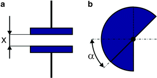
Schematic diagram of a capacitive transducer of linear displacement (a) and angular displacement (b)
In the case of the schematic in Fig. 1.8a, the relationship C(x) is described by the following equation:
$$C = \frac{\varepsilon A} {4\pi x},$$(1.62)where ε is a dielectric constant, A denotes the active area of the capacitor, and x is the distance between capacitor plates.
In the case of the schematic from Fig. 1.8b we have
$$C = \frac{\varepsilon A} {4\pi d}\left (1 -\frac{\alpha } {\pi }\right ),$$(1.63)where d is the distance between the rotor plates of the capacitor.
Capacitive sensors allow for a change in the capacitance not only by changes in the distance between plates (Fig. 1.8a) but also by changes in the active area of the capacitor plates or by the application of different dielectrics, e.g., air, or a layer of material of a different dielectric constant between the plates of the capacitor. Changes in mechanical quantities are registered through changes in the capacitance and then measured in an electrical measuring system. Capacitive sensors are characterized by a small force required for the displacement of the moving electrode of the sensor. Moreover, they enable contactless measurement and possess a small moving-electrode mass and large sensitivity.
-
5.
Angular Velocity Transducers
An angular velocity transducer (Fig. 1.9) can be a mechanical part of a system, but, as distinct from the problems of the mechanics of a rigid body described so far, here we address the mechanics of fluid flow (a hydraulic transducer or gas flow transducer).
Fig. 1.9 
Transducer for measurement of angular velocity ω
The measured angular velocity of shaft 3 is transmitted onto a paddle mixer 1 connected to casing 2. The pressure of a gas or liquid p 0 entering the working part of the angular velocity sensor passes through the paddle mixer, and at a hole in the casing the pressure p is seen, described by the equation
$$p = {p}_{0} + \frac{\rho } {2g}{\omega }^{2}\left ({r}_{ 2}^{2} - {r}_{ 1}^{2}\right ),$$(1.64)where ρ is the density of the medium
-
6.
Temperature Transducers
In this case, the change in resistance of a conductor R Θ is associated with a change in temperature Θ according to the equation
$${R}_{\theta } = {R}_{0}\left (1 + \alpha \left (\theta - {\theta }_{0}\right )\right ),$$(1.65)where R 0 is the resistance of the conductor at temperature Θ 0. The coefficient α[ ∘ C − 1] for iron is equal to 0. 002–0. 006, for aluminium 0. 0045, and for carbon 0. 0007.
Such a direct temperature measurement using temperature sensors called thermometers can span a range from − 170 ∘ C to 700 ∘ C.
Also in use are thermistors, that is, semiconductors of large temperature coefficients of resistance. The dependency of resistivity (a specific resistance) of a thermistor on temperature is described by the equation
$${\rho }_{\theta } = {\rho }_{0}{e}^{\left (\alpha \left /\right. \theta -\alpha \left /\right. {\theta }_{0}\right )},$$(1.66)where ρ0 and ρ Θ are the resistivities of a resistor corresponding to temperatures Θ 0 and Θ measured in degrees Kelvin, and α is a constant ( ∼ 4, 000). Thermistors are used to measure temperature in a range of 60 ∘ C − 120 ∘ C with an accuracy of up to 0. 0005 ∘ C.
-
7.
Thermocouples
Thermocouples are used in various kinds of automatic control systems for the measurement of temperature. A thermocouple consists of two conductors, welded together, of different properties of resistance change vs. the measured temperature, e.g., one electrode is made of pure platinum and the other is an alloy of platinum (90%) and rhodium (10%). Such thermocouples can be used to measure temperatures reaching up to 1, 600 ∘ C.
If two metals 1 and 2 are joined together (Fig. 1.10) and their points of contact A 1 and A 2 are at different temperatures Θ 1 and Θ 2, then four thermoelectric forces e will appear in the closed circuit. “Cold” ends of the thermocouple are connected to the system of potentiometers, and the “hot” end is in contact with a medium (an element) whose temperature is to be measured.
Fig. 1.10 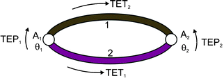
Two conductors joined together (the thermocouple) and four thermoelectric forces
Undesirable changes in ambient temperature affecting the cold ends of a thermocouple are compensated by introducing a bridge with a thermometer R t that measures the temperature of the cold ends.
The force TEP i is the Peltier thermoelectric force at the junction A i and the force TET i is the Thomson thermoelectric force in the wire i (i = 1, 2). The net thermoelectric force is equal to
$$TE = TE{P}_{1} - TE{P}_{2} + TE{T}_{2} - TE{T}_{1}.$$(1.67)Because of difficulties in the identification of particular Peltier and Thomson thermoelectric forces, the following equation is used:
$$TE = TE\left ({\theta }_{1}\right ) - TE\left ({\theta }_{2}\right ),$$(1.68)where TE(Θ 1) is the thermoelectric force at point A 1 (temperature Θ 1) and TE(Θ 2) is the thermoelectric force at point A 2 (temperature Θ 2).
In practice two metals 1 and 2 are used for temperature measurement by means of their connection to a meter (e.g., a millivoltmeter). In this way, an additional metal 3 is introduced into the circuit, and the measuring wires and internal circuit of the meter are made of this third metal (Fig. 1.11).
Fig. 1.11 
A thermocouple (1, 2) forming a circuit with metal 3
The thermoelectric force in the circuit shown in Fig. 1.11 is equal to
$$TE = T{E}_{12}\left ({\theta }_{1}\right ) + T{E}_{23}\left ({\theta }_{0}\right ) + T{E}_{31}\left ({\theta }_{0}\right ).$$(1.69)Because for Θ = Θ 0 we have TE(Θ 0) = 0, from (1.69) we obtain
$$T{E}_{23}\left ({\theta }_{0}\right ) + T{E}_{31}\left ({\theta }_{0}\right ) = -T{E}_{12}\left ({\theta }_{0}\right ).$$(1.70)Substituting (1.70) into (1.69) we obtain
$$TE = T{E}_{12}\left ({\theta }_{1}\right ) - T{E}_{12}\left ({\theta }_{0}\right ).$$(1.71)The preceding equation holds on the condition that the introduction of a third metal into the system composed of metals 1 and 2 does not affect the value of the net thermoelectric force and both ends of metal 3 are at the same temperature.
The oldest, simplest, and the most commonly used system of thermoelectric thermometer in industry is the schematic of the so-called swing thermometer shown in Fig. 1.12.
Fig. 1.12 
Swing system applied to temperature measurement
In the schematic in Fig. 1.12, 1 and 2 denote thermoelements, 1′ and 2′ are compensating wires, R w is the compensating resistor (selected in such a way that the external resistance of the meter R z = R zn , where R zn is the nominal resistance of the meter, calibrated in degrees Celsius), and M is a millivoltmeter. The millivoltmeter M measures the voltage U, which is equal to
$$U = ET \frac{{R}_{m}} {{R}_{z} + {R}_{m}},$$(1.72)$${R}_{z} = {R}_{12} + {R}_{1^{\prime}2^{\prime}} + {R}_{3} + {R}_{w},$$(1.73)where R 12 is the resistance of thermoelements 1 and 2, R 1′2′ is the resistance of compensating wires 1′ and 2′, R 3 is the resistance of connecting wires 3, and ET denotes the thermoelectric force of a thermoelement at the measured temperature Θ 1 and reference temperature Θ 0.
-
8.
Pressure Transducers
Transducers for pressure measurement can be divided into two types. The first type includes transducers whose principal working elements are mechanical elastic elements, the deformations of which are transformed into electrical signals using capacitive elements, inductive elements, or strain gauges.
The second type includes transducers where the main working elements are magnetoelastic cylinders.
Figure 1.13 shows examples of sensors of the first type for measurement of pressure of a flowing gas (a) and liquid (b).
Fig. 1.13 
Schematic diagram of pressure sensor of a flowing gas (a) and flowing liquid (b)
The bellows sensor for pressure measurement of a gas consists of a tube of undulating shape (a bellows) 1, a rack 2, and a pinion 3 connected to the terminal of the potentiometer 4. The pressure p causes stretching of the bellows 1 and displacement of the rack 2, and consequently a change in position of the potentiometer terminal, which leads to a change in output voltage U w . On the assumption that the relationship U w (p) is linear, the equation connecting the output voltage and the pressure has the form
$${U}_{w} = \alpha p,$$(1.74)where α is a proportionality factor. Displacement of the rack x can be determined after solution of the following second-order differential equation:
$$M\ddot{x} + c\dot{x} + kx = Ap,$$(1.75)where M denotes the mass of moving parts of the sensor, c is the viscous damping coefficient, k denotes bellows stiffness, and A is the cross-section area of the bellows. The problem can be reduced to a model of second-order inertial elements of the form (see Chap. 6 of [3])
$${T}^{2}\ddot{x} + 2\xi T\dot{x} + x = \alpha p,$$(1.76)where \(T = \sqrt{\frac{M} {k}}\), \(\xi = \frac{c} {2\sqrt{kM}}\), \(\alpha = \frac{A} {k}\), and the right-hand side of this equation is equal to U w [see (1.74)].
Equation (1.76) describes also the dynamics of the meter from Fig. 1.11b, and in this case the bellows is filled up with a liquid.
-
9.
Magnetoelastic Sensors
In Fig. 1.14 the schematic of a magnetoelastic element of a (second type) transducer for pressure measurement is shown.
Fig. 1.14 
Magnetoelastic element of a pressure sensor
Axial forces acting on a ferromagnetic element cause a change in the magnetic permeability of this element. The steel pipe 1 was covered with a pipe made of invar alloy. Inside was placed a choking coil 3. The pressure p causes expansion of the pipe 2, which leads to a change in the magnetic permeability of invar μ, which in turn affects the value of self-inductance of the coil according to the equation
$$L = 0.4\pi {N}^{2}1{0}^{-8}\frac{\mu A} {l},$$(1.77)where N is the number of coil turns, A denotes the cross-section area of the invar pipe, and l is its length. The coil is connected to a bridge, and the change in inductance of the coil results in a change in current intensity proportional to the pressure magnitude.
The measuring ammeter can be directly calibrated in units of force. Magnetoelastic sensors are also used for the measurement of large static and dynamic forces. The magnetoelastic effect apart from the aforementioned invar is also characteristic of nickel, permalloy, and iron.
-
10.
Piezoelectric Transducers
The piezoelectric effect discovered in 1880 by Marie and Pierre Curie consists in the generation of electric charges on faces of crystals loaded with tensile or compressive forces (e.g., quartz, Seignette’s salt, or barium titanate).


In Fig. 1.15 the frequency response of a piezoelectric sensor is shown. Because the force acting on a sensor plate is usually produced by a moving element of mass m, the signal obtained from the sensor is proportional to the acceleration of this element. The operating range of the sensor is 1–300 Hz, and the resonance frequency of this sensor is equal to about 30 kHz.

Frequency response of a piezoelectric sensor
Piezoelectric sensors have a very wide range of application for the measurement of frequency and acceleration. Their disadvantage is the requirement of dynamic calibration.
The application of piezoelectric transducers is broad, but here we will limit ourselves to determining the loss of energy of fluid flow on the basis of determining the difference in propagation velocity of ultrasonic vibrations. Figure 1.16 shows a schematic of measurement of energy loss of the fluid flowing in pipe 3 with velocity ν between two piezoelements 1 and 2 separated by distance l.

Measurement of flow energy losses by means of piezoelements
The generator G and the phase amplifier are alternately switched in by a commutator K in such a way that the piezoelements act at first as transmitters (radiators) and then as receivers of energy.
The instantaneous voltage of the radiating piezoelement
and the instantaneous voltage on the receiving piezoelement is equal to
where T denotes the time it takes the ultrasonic wave to cover distance l.
The phase difference between a steady-state vibration regime (when the medium is stationary) and vibration of a fluid is equal to
and the difference between the standard vibration and a vibration whose sense is opposite to the velocity of the fluid ν is equal to
where c is the velocity of propagation of ultrasound in the fluid and ν is the velocity of the fluid.
The phase difference is equal to
for c ≫ ν. The voltage of the piezoelement will be inversely proportional to velocity, that is,
where α is a proportionality factor. The values of current intensities in the amplifier are equal to
hence we calculate
where \(\beta = \frac{2{\alpha }_{1}} {\alpha }\) is a proportionality factor. From this the conclusion follows that for a constant volume of the pipe through which the fluid flows, losses of the flow will be proportional to the velocity of the flowing fluid.
1.2.2 Magnetic Force in a Single Mechatronic System
This problem was already partly considered in the section concerning inductive transducers. Let the single mechatronic system consist of a magnet core (1) with wounded coil of N turns (2), and armature (3), shown in Fig. 1.17.

Schematic diagram of a magnetic circuit in system of core (1), armature (3), and two air gaps

B(H) dependency for ARNON material used for transformer plates
The aim of these considerations is the determination of a magnetic force that attracts the armature (3) to the electromagnet (1) as a function of the current intensity I in the coil, the width of the air gap x, the cross-section area of core A, the length of the ferromagnetic part of the magnetic circuit l r , and the number of turns of coil winding N. We will neglect the hysteresis phenomenon in the core and assume the magnetic permeability of the air to be equal to magnetic permeability of vacuum. The magnetic induction B(T) generated in the circuit depends on the magnetic field H[A∕m], for example, as presented in Fig. 1.18.
Let us note that the function B(H) is bijective, making it is easy to build the inverse function H(B). The aforementioned non-linear functions can be described after the introduction of relative permeability μ = μ(B) or μ = μ(H), and the function B(H) takes the form
where μ0 is the vacuum permeability and is equal to \({\mu }_{0} = 4\pi \cdot 1{0}^{-7}\) \([ \frac{\mathrm{Vs}} {\mathrm{Am}}]\). A sample plot of the function μ(H) is shown in Fig. 1.19.

Example of μ(H) dependency for ARNON material
Let us note that lim H → ∞ μ(H) = 1. From Kirchhoff’s voltage law for a magnetic circuit from Fig. 1.18 we obtain
where R sz (R r ) denotes respectively the reluctance of two air gaps (reluctance of the ferromagnetic core and the armature) and Φ = Φ[Tm2] is the magnetic flux, assumed to be uniform at each point of a magnetic circuit.
From (1.87) we obtain
hence
Because the magnetic flux
from (1.91) and (1.90) we obtain
Equation (1.92) is a non-linear algebraic equation, where for fixed parameters we determine function B by means of numerical calculations. From (1.92) and exploiting (1.86) we obtain
Knowing function H [determined numerically from (1.93)] we determine its corresponding value of magnetic induction from (1.86).
Assuming a uniform magnetic field strength in the air gap, denoted H 0, the potential energy accumulated in the gap is equal to
The desired force acting on the armature is equal to
where during transformations (1.86) and the value μ(H 0) = 1 were used.
The relationship B(H) presented in Fig. 1.18 and the so-called phenomenon of magnetic polarization of the coreB p as a function of H allow for the introduction of a bilinear magnetization curve. Since it turns out that with an increase of H polarization increases linearly and after passing the value H s, the value of the polarization reaches a constant value B p = B s p for H ≥ H s [1]. Assuming a simplified magnetization model, both B(H) and B p(H) have the bilinear characteristics shown in Fig. 1.20.

Bilinear characteristics of B p(H) and B(H)
Piecewise linear changes in magnetic induction B(H) and B p(H) allow for the introduction of the following simplified equation:
The quantities H s (saturation magnetic field strength), B s p (saturation polarization), and B s (saturation induction), shown in Fig. 1.20, can be taken as material constants. Finally, the approximation of characteristics B(H) can be conducted based on two material constants B S and H S , and its bilinear approximation has the form
To point B S (H S ) corresponds \({\mu }_{S} = \frac{{B}_{S}} {{\mu }_{0}{H}_{S}}\), and the relative permeability μ = μ(H) is described by the two equations
shown in Fig. 1.21.

Function of relative magnetic permeability μ(H) corresponding to the bilinear magnetization curve
Kirchhoff’s voltage law when the bilinear approximation is used will take the following form:
The desired magnetic force is equal to
The simplification often used during the analysis of electromagnetic circuits is the assumption that 2xμ ≪ l r , which in many cases is justified, especially for small values of x. In this case from (1.93) we obtain
and in turn from (1.92) we get
The force acting on the armature, according to (1.95), is equal to
According to Kirchhoff’s voltage law, the relationship between the voltage supplying the circuit U and the current intensity in circuit I has the form
where R is the resistance of the winding.
However, in the case under consideration, now changes in the magnetic flux Φ are the result of changes in both the current intensity and the width of the air gap x. Differentiating (1.91) we have
where, according to (1.102), we have
Complete coupled non-linear algebraic-differential equations describing the electromagnetomechanical (mechatronic) circuit from Fig. 1.17 have the form
and the force F acting on the armature is described by (1.95). If the field strength H is proportional to the current intensity I, then the preceding (1.107) are reduced to one equation of the form
where U = U(t) is the voltage applied to the mechatronic system. The force F exerted by the electromagnet on the armature is described by (1.103), where the function μ = μ(I) occurs in the denominator.
1.3 Magnetic Levitation
Magnetic levitation is a known topic and can be realized in several ways [4–6], but the most spectacular effects can be observed when an electromagnet made of superconductor is used. A simpler way to create a system for the investigation of the levitation phenomenon is to use a system with an infrared light sensor (barrier) that traces the position of the levitating mass placed in the magnetic field generated by the electromagnet.
For the purpose of the experiment presented here the role of sensor is played by the infrared light barrier, which traces the actual position of the cylindrical mass (Fig. 1.22). The development toward future applications of fast and accurate position control systems used in optoelectronics, computer hardware, precision machining, robotics, and automotive has stimulated high-level engagement in the creation of non-conventional implementations [6, 7]. In this section, a numerical analysis devoted to that domain concerning non-contact (frictionless) fixing of some cylindrical mass in an alternating magnetic field is carried out [8]. The calculations given are an introductory step to the identification of electromagnet parameters and magnetic fields in the experimental realization of the problem, shown in Fig. 1.22. The mass levitates in the field generated by the electromagnet system supplied by a voltage of 12 V. Next to the numerical algorithm of voltage feedback there a modified PID control [7] of transient oscillations of the levitating light mass was also used. These were recorded until it reached a stable equilibrium position. The results of the experiments are presented on time plots of displacement h(t) measured between the opposite facing surfaces of the electromagnet core and the top surface of the levitating mass.

Schematic block diagram of hardware, signal connections, and levitating solid body
1.3.1 The Analyzed System
The electronic part of the system uses two light-sensitive resistors, the first one of which acts together with an infrared-light-emitting diode as a simple barrier tracing the cylindrical solid body position. Due to the existence in the surrounding space of many infrared-light-emitting sources such as the sun or lightbulbs (producing disturbance signals to the barrier), the second resistor measures the amount of light coming into the system from the surrounding space. If the barrier sensor is only partially illuminated (the result of being obstructed by the levitating body), the voltage difference appears and is input to the differential amplifier for the generation of the updated value of voltage supplying the electromagnet circuit. Experimental realization of the schematic diagram presented in Fig. 1.22 is shown in Fig. 1.23.

Experimental setup of control system of levitating cylindrical light mass (constructed by Piotr Jȩdrzejczyk, student of second-degree studies at the Faculty of Mechanical Engineering of the Technical University of Lodz, Poland)
The system shown in Fig. 1.23 can be modeled by a dynamical system of three first-order differential (1.109) describing the motion of the mass levitating in magnetic and gravitational fields and the voltage equation for the electric circuit with alternating current. The meaning of the elements of the system-state vector x is as follows: x 1 → h is the displacement of the levitating mass measured downward from the electromagnet surface, x 2 → dh ∕ dt the corresponding velocity of the displacement, and x 3 → i the electric current in the electromagnet electric circuit.
The governing equations follow:
where the electrical and physical constants are as follows: L = 0. 002 H is the coefficient of inductance, R = 0. 29 Ω the coefficient of resistance, \(k = 1{0}^{-4}\,\mathrm{kg} \cdot \mathrm{ {m}}^{2}/\mathrm{{C}}^{2}\), C the magnetic flux, m = 0. 0226 kg the mass of the levitating body.
1.3.2 Two Cases of Numerical Control
Voltage v(t) and force excitation u(t) are the two control signals. They are considered in two separate cases, namely: (1) u(t) is feedback from position h in the system with a PID controller having the transfer function \(\mathrm{PID}(s) = {k}_{P} + (s + {k}_{I})/s + {k}_{D}s\) inserted into the first axis of the block diagram shown in Fig. 1.24, while v(t) is a constant voltage source of 12 V; (2) a time-dependent control input voltage having the Laplace representation

Feedback from displacement of levitating mass in PID control for k P = 250, k I = 800, k D = 13
\(V (s) = -(({k}_{1} + {k}_{2}s + {k}_{3}{s}^{2})H(s) - {k}_{1}{h}_{0})\) to the analyzed dynamical system working as the plant in the closed-loop control system with feedback from the full state vector (a numerical model of the control strategy is shown in Fig. 1.25). Disturbances coming from any external light sources have been neglected.

Closed-loop input voltage control with use of full state-vector feedback for k 1 = 103, k 2 = 20, k 3 = { 0. 0, 0. 2} in a model made in Simulink
Both of the numerical models presented contain characteristics of the operation of an infrared light barrier \(\mathrm{IRR}(t) = 1 - {b}_{\mathrm{IRR}}h{(t)}^{-2}\). This approximation with damping (sensitivity) constant b IRR measures the amount of infrared light transferred from the emitting diode to the light-sensitive resistor with the levitating body serving as the barrier.
Figure 1.26 shows the well-studied effect of introducing an infrared light barrier. The case for a short range of values of the IRR factor was described as the correct one, being more realistic in relation to the motion of mass m observed on the experimental rig. During this experiment one tries to fix the mass at height h f = 1 cm with the initial condition h 0 = 3 cm. It is clear that the mass is quickly attracted to the steady-state position but is achieved in a different manner.

Time plots of h(t) obtained from diagram shown in Fig. 1.24 for different values of the infrared light barrier factor \({b}_{\mathrm{IRR}\{1,2,3\}} =\{ \mathrm{IRR\ off},\,0.7 \cdot 1{0}^{-4},\,0.4 \cdot 1{0}^{-4}\}\) in the closed-loop position feedback control and for h 0 = 3 cm
Frictionless oscillations in the transition to a stable position can be damped very well (Fig. 1.27) with the use of the second case of the control strategy based on feedback from the full state vector, as shown in Fig. 1.25. For a different initial position (h 0 = 2 cm) of mass m there is visible a quicker (because of the voltage, not external force feedback, as examined in the first approach) and better damped attraction of the mass to the steady-state position. With respect to application of a different method of control (with a control with feedback to the voltage time variable input v), the whole system is characterized by a slightly different dynamics, so the position of convergence changes with the use of larger values of \({b}_{\mathrm{IRR}\{1,2,3\}} =\{ 7,\,0.7,\,22.2\} \cdot 1{0}^{-4}\). Factor b IRR{3} is the highest available here, and the control nicely fixes the levitating mass at h 3 = 1. 67 cm. At this position the stabilized voltage supplying the electromagnet equals 13.66 V. The time plot of h 4 in Fig. 1.27 is an unnatural effect of a non-zero coefficient of feedback from acceleration (k 3 = 0. 2; see Fig. 1.25). The desired position is achieved in about 1.2 s, and it confirms that the vector component of feedback from acceleration is not necessary in this application.

Time plots of h(t) evaluated from diagram shown in Fig. 1.25 for different values \({b}_{\mathrm{IRR}\{1,2,3\}} =\{ 7,\,0.7,\,22.2\} \cdot 1{0}^{-4}\) corresponding to h {1, 2, 3} (for k 3 = 0), respectively. Infrared light sensitivity factor b IRR{4} = b IRR{3} (for k 3 = 0. 2), and h 0 = 2 cm
Depending on the presence of an IRR light barrier and the values of its sensitivity factor (b IRR), various shapes of the step response can be distinguished. The convergence is quite fast and well damped when the IRR light correction exists and, additionally, takes a correct value of its significance. The choice of incorrect value of b IRR results in the mass being brought into small-amplitude, weakly damped oscillations about its desired steady-state position. In some conditions, such an effect is observable also at a real laboratory rig and is undesirable if we need to fix the levitating mass at a constant height. Therefore, the introduced feedback from the infrared light barrier with mass m working as the armature of the electromagnet is justified. Better shapes of characteristics of the transition to steady-state responses were confirmed by the second control strategy. They are faster and more stable, and no oscillations are reported after examination of system parameters. The magnetic field allowed for elimination of any kinds of friction that are usually required in various realizations of fixings. Our experimental investigations will turn to the identification of electromagnetic parameters of the complete mechatronic system and the associated magnetic field. This is expected to help improve both the numerical adequacy of the presented approach and the tested strategy of control.
1.4 String-Type Generator
The dynamics of non-linear discrete-continuous systems governed by ordinary differential equations and partial differential equation often causes difficulties in numerical analysis. The reason lies not only in non-linear terms but mainly in time-consuming numerical techniques used to find the solution of the partial differential equations. Furthermore, usually real physical systems possess many parameters that can be changed over wide regions, and in practice direct simulation of the governing equations is costly and very tedious. Sometimes it does not provide physical insight into the obtained results. A deeper understanding of the dynamical behavior of the system under consideration can be discovered by the application of appropriate scaling and the proper use of averaging techniques [9–11]. In this section the electromechanical system under consideration serves as an example for a systematic strategy for solving many other related problems encountered in non-linear mechanical, biological, or chemical dynamical systems. First, an averaging method is proposed that is supported by a program for symbolic computation, and then further systematical study of the obtained ordinary differential equations is developed.
1.4.1 Analyzed System
The electromechanical model under consideration consists of a distributed mass system (string) whose oscillations are governed by a PDE (a detailed discussion of the model is given in [12–14]). The string is embedded in the magnetic field and crosses a magnetic flux perpendicularly (Fig. 1.28a). On the other hand, the string is made of steel and has its own inductance L, resistance R, and capacitance C. It appears that the equilibrium position of the string is unstable. The existence of the magnet induction and movement of the string causes the occurrence of voltage and then of a current in the string. The amplitude of the current undergoes change controlled by the amplifier with a time delay. Figure 1.28b shows the schematic of the electric system. The output and input voltages are governed by a non-linear cubic-type relation.

Scheme of string embedded in magnetic field (a) and electrical model (b)
The magnetic induction B(x) acting along the string generates voltage at the ends of the string according to the following equation:
where x is the spatial coordinate, t denotes time, u(t, x) is the string displacement in the point (t, x), and l is the length of the string. The amplifier gives the output voltage
where \(\widetilde{{h}}_{i}\) (i = 1, 2) are constant coefficients.
The current oscillations, including a time delay τ in the amplifier, are governed by the equation
where
and the dot denotes differentiation with respect to t and I(t) denotes the changes of the current. The changes in time of I(t) and the changes in x of B(x) play the role of force acting on the string whose oscillations are governed by the equation
where h 0 is the external damping coefficient, ρ is the mass density along the unit length, and ε is the small positive parameter.
The frequencies of free oscillations of the string are given by \({\omega }_{s} = \pi cs/l\), and the homogeneous boundary conditions are as follows:
1.4.2 Averaging Method
Our consideration is limited to first-order averaging. For ε = 0 the solution to (1.113) can be approximated by
where a 1, a 3 are the amplitudes, and θ1, θ3 the phases.
Only two modes are taken into account because the others are quickly damped during the string dynamics and their influence on the results can be neglected.
For a small enough ε≠0 the solution to (1.113) is expected to be of the form
Supposing that B(x) is symmetric with respect to the ends of the string, i.e., \(B(x) = B(l - x)\), we take
This assumption clarifies the selection of modes in (1.115). From (1.110) we obtain
and the right-hand side of (1.112) is calculated using a symbolic calculation (in Mathematica)
where
From (1.119) we take only the harmonics siniω1 t, cosiω1 t (i = 1, 3), and therefore
where
A solution to the linear (1.112) has the form
where M i , N i are given below:
and the abbreviation h. h. denotes higher harmonics that are not taken into account.
Further analysis is straightforward for the perturbation technique, and the details can be found elsewhere [9, 15]. Because B(x) and I(t) are defined, (1.113) can be solved using a classical perturbation approach. (It is assumed that u 1(x, a 1, a 3, θ1, θ3) is a limited and periodic function).
Substituting (1.116) into (1.113) and taking into account that a i = a i (t) and θ i = θ i (t) (i = 1, 3) are slowly changing in time, from the right-hand side of (1.113) (henceforth referred to as R) the following resonance terms are computed:
where R ic , R is correspond to the terms by cosψ i0 and sinψ i0, respectively. The comparison of the terms by cosψ i0 and sinψ i0 and generated by the left-hand side of (1.113) to those defined by (1.125) leads to the following average-amplitude equations:
The preceding equations are coupled via (1.122). The first attempt to derive an averaged set of equations was made by Rubanik [12]. However, neither qualitative nor quantitative analysis or predictions of the possible behavior of the solutions to the equations obtained have been given.
The analyzed set of equations has some properties that can cause difficulties during numerical analysis. First of all, this is a stiff set of equations [note the occurrence of a i (i = 1, 3) in the denominator of the last two equations of (1.126)]. As is assumed by the averaging procedure, amplitudes a i and θ i change in time very slowly, and a long integration to trace the behavior of the system is required.
For the further analysis of the time-dependent solutions we transform (1.126) into amplitude equations. For this purpose we assume
The comparison with (1.115) yields the following relations:
In what follows the set of amplitude differential equations has the form
where \(\dot{{a}}_{i}\) and \(\dot{{\theta }}_{i}\) are given by (1.126) and
1.4.3 Numerical Analysis and Results
In a standard approach to non-linear dynamical system analysis, time-dependent solutions are first considered and examined. For this purpose we consider a non-linear set of algebraic equations obtained from (1.126), where the left-hand sides are equal to zero. To solve the problem, a Powell hybrid method and a variation of Newton’s method were used. They require a finite-difference approximation to the Jacobian with high-precision arithmetic. The root was accepted if the relative error between two successive approximations was less than 0. 0001.
In a general case it can happen that the system of equations under consideration has one isolated solution or has a family of coexisting solutions for a fixed set of parameters. The system always possesses the trivial solution \({a}_{1} = {a}_{3} = {\theta }_{1} = {\theta }_{3} = 0\), which corresponds to the equilibrium position of the original system. Non-trivial solutions correspond to the periodic oscillations of the string described by the assumed solution (1.116). The stability of periodic oscillations corresponds to the stability of fixed points, i.e., to the stability of roots of the non-linear algebraic equations. To define the stability of the time-independent solutions obtained from the algebraic non-linear set of equations, we perturb them and then substitute for (1.116). Taking into account only the first powers of perturbations we get from (1.116) a linear set of differential equations. Based on these equations, a matrix corresponding to the analyzed fixed point is defined. In our case, because of the complicated equations, that matrix is obtained numerically. The eigenvalues of the matrix obtained determine the stability and bifurcation of the analyzed solutions (see monographs [16, 17]).
We present below two examples of such a computation. The following parameters were treated as fixed: l = 0. 1, ω = 4. 1, λ = 0. 01, k = 25, h 1 = 0. 01, h 2 = 0. 6, \(\epsilon /\rho = 1\), h 0 = 0, B 3 = 0. 4. The coefficient μ and the amplitude B 1 served as the control parameters. In Fig. 1.29 one can observe that for μ = 0. 001 with an increase in the first amplitude of the electromagnetic induction, the amplitude a 1 decreases (the amplitude a 3 and the phases θ1 and θ3 remain almost constant). A similar situation is observed for μ = 0. 01 and μ = 0. 1. This means that for the considered set of fixed parameters, an increase in B 1 damps the magnitude of oscillations.

First harmonic amplitude against B 1
A question arises as to whether there is only one isolated solution that corresponds to the fixed value of B 1. We have found that in an interval B 1 ∈ (3. 0, 5. 0) for each value of B 1 there exist two solutions for a 1 (marked with triangles) and one for a 3 (marked with crosses), as shown in Fig. 1.30. In both figures the obtained solutions are stable.

Example of multiple set of solutions corresponding to B 1 = 4. 5
It is a difficult task to prove the existence of time-dependent solutions in the system of averaged (1.129). The most expected situation (confirmed by numerical computations) is to find stable fixed points that correspond to the oscillations with constant amplitudes in the original system. However, we have also found periodic orbits in the analyzed averaged differential equations. On the basis of this example, it is proper to describe the benefits obtained from the averaging technique applied. Instead of examining of a complicated system of non-linear partial and ordinary differential equations, we reduce the problem to the analysis of the four ordinary differential equations. Inserting the results obtained numerically into (1.127) we obtain an averaged solution corresponding to the original system.
We now briefly describe a numerical method for tracking down changes in periodic orbits, their stability, and potential bifurcations [16, 17]. For this purpose, let us consider an approximate position of the fixed point Y 0 (k) close to the unknown exact one and perform numerical integration over the estimated period T (k). Actually, we have rescaled the equations according to the rule \(\overline{t} = \Omega t\), where Ω serves as an unknown to be determined and the period is equal to 2π. The error \(E = {Y }_{0}^{(k)} - {G}_{0}^{(k)}\) (where G 0 (k) = G(Y 0 (k)) is a point mapping) shows the accuracy of the calculations. Then, after a perturbation of the fixed point, its stability is determined based on the eigenvalues of a monodromy matrix. The results of calculation of the fixed points of the map (periodic orbits) as functions of B 1 for l = 0. 1, μ = 0. 1, ω = 2. 9, λ = 0. 1, k = 9. 0, h 1 = 0. 05, h 2 = 0. 01, \(\rho /\epsilon = 1.0\), h 0 = 0. 02, B 3 = 0. 8 are presented in Fig. 1.31a, b. In this figure, Y 3 and Y 4 are much smaller than Y 1 and Y 2 and are assumed to be zero. Variation of the period following the change of B 1 is evident (Fig. 1.31b, where \(Z = 1/\Omega \)). The observed periodic orbit is “strongly” stable because the corresponding multipliers lie close to the origin. As an example, one of the periodic orbits is presented in Fig. 1.32a, b. One revolution of the variables Y 1, 2 corresponds to two revolutions of Y 3, 4 during the period 2π.

Fixed points of Y 1, Y 3, Y 4 (a) and \(Z = 1/\Omega \) (b) against control parameter B 1

Periodic orbits Y 1, 2 (a) and Y 3, 4 (b) with normalized 2π period
Special attention is focused on detecting the time-dependent aperiodic solutions to the averaged equations. Some interesting non-linear phenomena will be discussed subsequently and illustrated based on the gear simulation of the averaged equations.
Let us first consider the following fixed parameters: l = 0. 1, μ = 0. 15, ω1 = 190, λ = 0. 1, k = 25. 0, h 1 = 0. 58, h 2 = 0. 05544, ρ = 1. 0, ε = 0. 05, h 0 = 0. 001, B 3 = 0. 08. Here the coefficient μ serves as a control parameter. Figure 1.33a illustrates the oscillations of Y 1, 2 and the exponential decay of Y 3, 4. The variables Y 1, 3 and Y 2, 4 correspond to the time evolution of the first two modes of the string arid their derivatives, respectively.

Time evolutions of amplitudes: (a) μ = 0. 15, (b) μ = 0. 125
The amplitudes of the first mode oscillate, but those corresponding to the third mode decrease in time in a non-oscillatory (exponential) manner. The decrease in μ damps the oscillatory effects, which is shown in Fig. 1.33b for μ = 0. 125.
Figure 1.34 (l = 0. 1, μ = 0. 0, ω1 = 900. 0, λ = 0. 1515, k = 2750. 0, h 1 = 5. 48, h 2 = 70. 0, ρ = 1. 0, ε = 0. 009, h 0 = 0. 00001, B 1 = 0. 65, B 3 = 0. 89) illustrates an unexpected non-linear phenomenon. A long time-transitional process has been interrupted by the sudden occurrence of the strong nonlinear Y 1, 2 oscillations.

Strong non-linear oscillations of amplitudes

Amplitude versus time

Independent transitional time evolution of amplitudes leading to instability
In Fig. 1.35 the coexistence of the periodic oscillations Y 1, 2(t) with the exponential decay of Y 3, 4(t) is shown. The simulation was performed for the following fixed parameters: l = 0. 1, μ = 0. 1, ω1 = 0. 1, λ = 0. 1, k = 7250. 0, h 1 = 0. 1, h 2 = 0. 1, ρ = 1. 0, ε = 0. 05, h 0 = 0. 001, B 1 = 6. 3, B 3 = 0. 08. Because Y 1, 2 and Y 3, 4 correspond to the first and third modes of the string, respectively, this result can be interpreted as the independent mode behavior.
The result obtained also illustrates another interesting non-linear behavior. The solution to the averaged non-linear differential equations can be assumed analytically in a different form: an exponential decay function and an oscillatory function with a constant amplitude.
Figure 1.36 (l = 0. 1, μ = 0. 1, ω1 = 190. 0, λ = 0. 1, k = 25. 0, h 1 = 0. 58, h 2 = 0. 05544, ρ = 1. 0, ε = 0. 005, h 0 = 0. 00999, B 1 = 6. 3, B 3 = 0. 08) presents a strange time evolution leading to instability. Here also Y 1, 2(t) increases with oscillations, while Y 3, 4(t) slightly decreases almost linearly. After a long transitional state, barrierlike phenomena appear. Finally, strong nonlinear pressing effects, leading to the vertical unlimited increase in Y 1, 2(t), are observed.
This behavior can be explained as follows. An almost linear decrease in Y 3, 4(t) leading asymptotically to zero causes the occurrence of a sudden increase in Y 1, 2(t) due to the existence of a 3 in the denominator of the last equation of (1.126). However, typically the system does not exhibit such instability effects.
Finally, consider the following set of fixed parameters: l = 0. 1, μ = 0. 00001, ω1 = 900. 0, λ = 0. 1515, k = 7250. 0, h 1 = 5. 48, h 2 = 65. 0, ρ = 1. 0, ε = 0. 009, h 0 = 0. 00001, B 1 = 0. 65, B 3 = 0. 23. A strong non-linear transitional oscillation of Y 1(t) is shown in Fig. 1.37. The variables Y 3, 4(t) again change in a non-oscillatory manner quite independently in comparison with the first oscillation mode.

Strong non-linear transitional oscillations
1.5 Rotor Supported by Magnetohydrodynamic Bearing
In general, rotating machinery elements are frequently encountered in mechanical/mechatronic engineering, and in numerous cases their non-linear dynamics causes many harmful effects, i.e., noise and vibrations. In particular, non-linear rotordynamics plays a crucial role in understanding various non-linear phenomena and despite its long research history (see, e.g., [18–22] and references therein), it continues to attract the attention of many researchers and engineers. Since the topics related to non-linear rotordynamics are broad ranging and cover many interesting aspects related to both theory and practice, in this section we aim only at the analysis of some problems related to a rotor suspended in a magnetohydrodynamic field in the case of soft and rigid magnetic materials.
Magnetic, magnetohydrodynamic, and piezoelectric bearings are used in many mechanical engineering applications to support a high-speed rotor, provide vibration control, minimize rotating friction losses, and potentially avoid flutter instability. Many publications are dedicated to the dynamic analysis and control of a rotor supported on various bearing systems. The conditions for active closed-/open-loop control of a rigid rotor supported on hydrodynamic bearings and subjected to harmonic kinematical excitation are presented in [23, 24]. The methodology for modeling lubricated revolute joints in constrained rigid multibody systems is described in [25]. The hydrodynamic forces used in the dynamic analysis of journal bearings, including both squeeze and wedge effects, are evaluated from the system-state variables and included in the equations of motion of multibody systems. To analyze the dynamic behavior of a rub-impact rotor supported by turbulent journal bearings and lubricated with couple stress fluid under quadratic damping, the authors of reference [26] used system-state trajectory, Poincar maps, power spectrum, bifurcation diagrams, and Lyapunov exponents. Dynamic motion was detected to be periodic, quasiperiodic, and chaotic.
Rotor-active magnetic bearing (AMB) systems with time-varying stiffness are considered in [27]. Using the method of multiple scales, a governing non-linear equation of motion for the rotor-AMB system with one degree of freedom is transformed into an averaged equation, and then bifurcation theory and a bifurcation method of the detection function are used to analyze the bifurcations of multiple limit cycles of the averaged equation.
Rotors supported by floating ring bearings may exhibit instabilities due to self-excited vibrations [28]. The authors applied linear stability analysis to reveal a sign change of real parts of the conjugated eigenvalue pairs, and a center manifold reduction approach allowed them to explain the rotor destabilization via Hopf bifurcation. Owing to the analytical predictions that were applied, both sub- and supercritical bifurcations were found, and the analytical results were compared with numerical ones using a continuation method. Observe that rotors supported by a simple fluid film bearing the so-called oil whirl and oil whip dynamics ad been studied analytically in [18, 20–23]. Additionally, this problem was reconsidered recently with respect to inner and outer oil films and synchronization [29]. The full annular rub motion of a flexible rotor induced by mass unbalance and contact rub force with rigid and flexible stators, taking into account dry friction between the stator and rotor, is studied in [30]. Stability and synchronous problems of full annular rub motions are discussed, and a simplified formula for the dynamic stability of the system being investigated is derived.
Ishida et al. [31] investigate the vibrations of a flexible rotor system with radial clearance between an outer ring of the bearing and a casing using numerical and experimental studies. The following non-linear behavior was detected, illustrated, and discussed: (a) sub-, super-sub, and combined resonances; (b) self-excited vibrations of forward whirling mode; and (c) transitions from self-excited to forced system vibrations. In particular, the influence of static force and bearing damping was analyzed using the harmonic balance method.
Quinn [32] studied the non-linear output of a damped Jeffcott rotor with anisotropic stiffness and imbalance. It was shown that for sufficiently small external torque (or large imbalance), resonance capture may occur whereby the rotational shaft velocity cannot increase beyond the fundamental resonance between the rotational and translational motion providing a mechanism for energy transfer. Prediction of the system behavior on the basis of the reduced-order averaged model is verified and validated against numerical studies of the original ODE-governed model.
In this section, the two-degree-of-freedom non-linear dynamics of a rotor supported on a magnetohydrodynamic bearing system (MHDB) is analyzed in the cases of soft and rigid magnetic materials. In the case of soft magnetic materials, the analytical solutions were obtained using the method of multiple scales [9, 15]. Rigid magnetic materials possess hysteretic properties that are realized in the present work by means of the Bouc–Wen hysteretic model [33, 34]. This model enables simulation of hysteretic loops of various forms for systems from very different fields such as mechanics, biology, electronics, ferroelectricity, and magnetism [35]. In particular, in mechanical/civil and mechatronic engineering, hysteresis occurs as the natural inclination of materials to yield to restoring forces against motion and dissipate energy, and it often deals with the memory nature of inelastic material properties, where the restoring forces (torques) depend on the deformation process history. In general, the classic Bouc–Wen model is described by the first-order non-linear ODE governing the input (displacement rotations) and output (restoring force/torque) signals in a hysteretic way. Furthermore, a proper choice of the Bouc–Wen parameters allows one to control their behavior so that it is similar to that of real hysteresis looplike processes. Observe that despite the simplicity of the Bouc–Wen model, its behavior and possible application still attract many researchers, in particular regarding the following topics:
-
(a)
Ways of tuning the Bouc–Wen control parameters to match application-oriented hysteretic material properties (identifications process).
-
(b)
Numerical analysis of a given full mathematical model including its control.
-
(c)
Rigorous mathematical background devoted to proofs of the convergence between the Bouc–Wen-like models and their real application-oriented counterpart dynamic objects.
An extensive list of references related to the Bouc–Wen model and beyond, together with results of the researches associated with the analysis, identification, and control of the Bouc–Wen-like models, are reported in the monograph by Ikhouave and Rodellar [36], where the following topics are illustrated and discussed: compatibility of the model versus physical laws, model parameters and hysteresis loops, identification and control of dynamic systems with Bouc–Wen models. Finally, various mathematical approaches to the hysteresis phenomenon are given in a survey reference [37].
As was demonstrated by investigations in [35], systems with hysteresis may reveal an unexpected behavior. On the one hand, hysteresis, like any dissipation, promotes the stabilization of motion and may restrain the occurrence of chaos. On the other hand, it may cause chaotic vibrations in a system. This last property is confirmed by the results of this section. In the absence of hysteresis, chaos is not observed. Taking into account hysteretic properties leads to chaotic vibrations of a rotor under certain conditions. The effect of hysteretic dissipation on the emergence of chaos is investigated using a methodology based on an analysis of wandering trajectories [33, 38]. Chaotic regions were obtained in parametric planes characterized by dynamic oil film action, magnetic control parameters, hysteretic dissipation, and the amplitude and frequency of external excitation.
1.5.1 Mathematical Model
Let us consider a uniform symmetric rigid rotor (Fig. 1.38) supported by a magnetohydrodynamic bearing system. The four-pole legs are symmetrically placed in the stator. F k is the electromagnetic force produced by the kth opposed pair of electromagnet coils. This force is controlled by electric currents
and can be expressed in the form
where i 0 denotes the bias current in the actuators’ electric circuits, μ0 is the magnetic permeability of vacuum, A is the core cross-section area, N is the number of windings of the electromagnet, δ is the air gap in the central position of the rotor with reference to the bearing sleeve, l is the total length of the magnetic path, the constant value \({\mu }^{{_\ast}}\,=\,{B}_{\mathrm{S}}/({\mu }_{0}{H}_{\mathrm{S}})\) denotes the magnetic permeability of the core material; the values of the magnetic induction B S and magnetizing force H S define the magnetic saturation level [23, 24]. θ k is the angle between axis x and the kth magnetic actuator, Q 0 is the vertical rotor load identified with its weight, and (P r , P τ) are the radial and tangential components of the dynamic oil-film action, respectively. The equations of motion of the rotor are represented in the following form [23, 24, 39]:
Here m ∗ denotes the rigid rotor mass, (x ∗ , y ∗ ) are the Cartesian coordinates of the rotor center, Q x ∗ (t), Q y ∗ (t) are the external excitation characterizing bearing movements. We consider the vibrations of the rotor excited by the harmonic movements of the bearing foundation in the vertical direction:
where Q ∗ and Ω ∗ are the amplitude and frequency of the external excitation, respectively. The constant C ∗ is defined as

Cross-section diagram of a rotor symmetrically supported on magnetohydrodynamic bearing
The parameters μ s , δ s , R c , and L c denote the oil viscosity, relative bearing clearance, journal radius, and total bearing length, respectively. (ρ, ϕ) are the polar coordinates, and \(p(\rho ) = 1 - {\rho }^{2}\), \(q(\rho ) = 2 + {\rho }^{2}\).
To represent the equations of motion in a dimensionless form, the following changes in variables and parameters are introduced:
where ω ∗ is the rotation speed of the rotor and c ∗ is the bearing clearance.
Thus the dimensionless equations of motion take the form
Here
and the magnetic control forces are expressed as follows
where (x 0, y 0) are the coordinates of the rotor static equilibrium and γ and λ are the control parameters.
1.5.2 Soft Magnetic Materials
In this section, we consider the two-degree-of-freedom dynamics of the rotor in the MHDB system without taking hysteresis into account.
1.5.2.1 Non-resonant case
The right-hand sides of (1.137) were expanded into Taylor series, and the origin was shifted to the location of the static equilibrium (x 0, y 0) for the convenience of investigation. The linear and quadratic terms were retained, so the reformed equations of motion are as follows:
We seek the first-order solution for small but finite amplitudes in the form
where ε is the small, dimensionless parameter related to the amplitudes and T n = εn t (n = 0, 1) are the independent variables; T 0 is the “fast” time, whereas T 1 is the “slow” time. It follows that the derivatives with respect to t become expansions in terms of the partial derivatives with respect to T n according to
where \({D}_{k} = \frac{\partial } {\partial {T}_{k}}\).
To analyze the non-resonant case the forcing term is ordered so that it appears at order ε. Thus, we recall in (1.140) F = εf, \(\hat{{\mu }}_{n} = \epsilon {\mu }_{n}\). Substituting (1.141) into (1.140) and equating the coefficients of similar powers of ε we obtain
Order ε
Order ε2
The solution of (1.143) is expressed in the form
where CC denotes the complex conjugate of the preceding terms, A 1 and A 2 are the arbitrary functions of T 1 at this level of approximation,
ω n are assumed to be distinct, and ω n 2 are the roots of the characteristic equation
Substitution of (1.145) into (1.144) gives
Terms that do not influence the solvability conditions are not presented in the last equations and were replaced by dots. To determine the solvability conditions of (1.144), following the method of undetermined coefficients we seek a particular solution in the form
with unknowns P 11, P 12, P 21, and P 22. Substitution of expressions (1.149) into (1.148) and collecting the coefficients at exp(iω1 T 0) and exp(iω2 T 0) yield
where
Taking into account the characteristic (1.147), the determinant Δ of the set of linear algebraic equations relative to P 1n , P 2n [(1.150)] is equal to zero:
According to the Kronecker–Kapelly theorem, the set of linear algebraic equations is compatible if and only if the matrix rank of the linear set is equal to the extended matrix rank. Therefore, the solvability conditions are
otherwise the set of linear algebraic (1.150) has no solutions. So
and the solvability conditions can be written in the form
The differential equations to define A 1(T 1) and A 2(T 1) are the consequence of solvability conditions (1.155)
It follows from (1.141), (1.145), and (1.156) that the complex solution of the differential set (1.140) is
Then the real solution is as follows:
where
and a n and Θ n are the real constants.
Figures 1.39–1.41 show a comparison of the numerical integration of (1.140) and the perturbation solutions (1.158) for the following parameters of set (1.140): α = 1, 500, β = 70, α1 = 9. 985 ×102, α2 = 2 ×10³, α3 = 7. 9588 ×103, α4 = 0. 002, \({\alpha }_{5} = -4.0794 \times 1{0}^{3}\), α6 = 4. 0002 ×103, α7 = 8. 0005 ×103, β1 = 29. 9975, \({\beta }_{2} = -0.001\), \({\beta }_{3} = -4.1594 \times 1{0}^{3}\), \({\beta }_{4} = -1.9997 \times 1{0}^{3}\), \({\beta }_{5} = -7.9188 \times 1{0}^{3}\), β6 = 0. 7959, \({\beta }_{7} = -0.4083\); the initial conditions are \(x(0) = 1{0}^{-12}\), \(y(0) = 1{0}^{-10}\), \(\dot{x}(0) =\dot{ y}(0) = 0\).
In the case of non-resonant undamped vibrations of a rotor (Fig. 1.39), it is accepted for numerical integration that \(\hat{{\mu }}_{1} = 0\), \(\hat{{\mu }}_{2} = 0\), F = 0. According to (1.158), the perturbation solution is presented by the expressions


Figure 1.40 corresponds to the non-resonant damped vibrations of a rotor. For this case, \(\hat{{\mu }}_{1} = 0.1\), \(\hat{{\mu }}_{2} = 0.15\), F = 0. The perturbation solution has the form
For the non-resonant forced damped vibrations of a rotor (Fig. 1.41) it is accepted for numerical integration that \(\hat{{\mu }}_{1} = 0.1\), \(\hat{{\mu }}_{2} = 0.15\), F = 0. 005, Ω = 10, \(\tau = -\pi /2\). The perturbation solution is
Figures 1.39–1.41 demonstrate good agreement of the numerical and analytical solutions.

1.5.2.2 Primary Resonance: The Cases of no Internal Resonance and an Internal Resonance
To analyze primary resonances, the forcing term is ordered such that it appears at order ε2 or in the same perturbation equation as the non-linear terms and damping. Thus, we recall in (1.140) F = ε2 f, \(\hat{{\mu }}_{n} = \epsilon {\mu }_{n}\). Consider the case where Ω ≈ ω2. The case Ω ≈ ω1 is analogous. Let us introduce the detuning parameter σ1 and set \(\Omega = {\omega }_{2} + \epsilon {\sigma }_{1}\).
Substituting (1.141) into (1.140) and equating coefficients of similar powers of ε we obtain
Order ε
Order ε2
The solution of (1.163) is given in the form
where
Substitution of (1.165) into (1.164) yields
Let ω2 > ω1 for definiteness. We need to distinguish between the case of internal resonance ω2 ≈ 2ω1 and the case of no internal resonance, i.e., ω2 is away from 2ω1. The case ω1 > ω2, ω1 ≈ 2ω2 is analogous. When ω2 is away from 2ω1, the solvability conditions (1.155) are written in the form
where
Thus, when there is no internal resonance, the first approximation is not influenced by the non-linear terms; it is essentially a solution of the corresponding linear problem.
Actually, the solutions of the differential equations below
are
where a n and Θ n are the real constants:
As t → ∞, T 1 → ∞, and
and according to (1.165), we obtain the following steady-state response:
Therefore, the real solution is
or it can be rewritten in the form
where \(\tilde{{\gamma }}_{1} =\arctan ({\nu }_{2}/{\sigma }_{1})\), \(\tilde{{\gamma }}_{2} = -\arctan ({\sigma }_{1}/{\nu }_{2})\).
Another situation occurs when the internal resonance ω2 ≈ 2ω1 exists. Let us introduce the detuning parameter σ2 and set
Taking into account (1.161), the solvability conditions for this case become
Here coefficients \({q}_{{\omega }_{1}}\), \({q}_{{\omega }_{2}}\), \({q}_{{\omega }_{2}-{\omega }_{1}}\), and \({q}_{2{\omega }_{1}}\) are the expressions in parentheses at the exponents with the corresponding powers (1.167) and \({p}_{{\omega }_{1}}\), \({p}_{{\omega }_{2}}\), \({p}_{{\omega }_{2}-{\omega }_{1}}\), and \({p}_{2{\omega }_{1}}\) are the expressions in brackets at the exponents with the corresponding powers (1.168):
For convenience let us introduce the polar notation
where a m and Θ m are the real functions of T 1. Substitution of (1.181) into (1.179) yields
In the preceding expressions the following notations were introduced:
and ν1 and ν2 are defined as in (1.158).
Separating (1.182) into real and imaginary parts and taking into account that according to (1.145) Λ n (n = 1, 2) is the imaginary value, we obtain
For the steady-state response \({a^\prime}_{n} = {\gamma^\prime}_{n} = 0\), therefore,
Two possibilities follow from (1.184). The first one is given by (1.174). It is the solution of the linear problem. Let us find functions a 1 and a 2 of T 1 according to the second possibility. It follows from the first two equations of (1.184) that
So
Let us take sinγ2 and cosγ2 using, for example, the formulas by Cramer:
where
Then a biquadratic equation relative to a 1 follows from the last two equations of (1.184):
Finally, we obtain the expression for a 1:
where
Thus, the unknown functions in (1.165) were defined. It follows from (1.141), (1.165), and (1.181) that
Then, the real solution is as follows:
Here a 1 and a 2 are defined by (1.187) and (1.191).
Let us consider the expression for a 1 (1.191). When
there are no real values of a 1 defined by (1.191) and the response must be given by (1.177). When
there is one real solution defined by (1.191). Therefore, the response is one of the two possibilities given by (1.177) and (1.194). When
there are two real solutions defined by (1.191). Therefore, the response is one of the three possibilities given by (1.177) and (1.194).
Figure 1.42 depicts frequency-response curves. a 1 and a 2 are plotted as functions of σ1 for σ2 = 0. The dashed line with a peak at σ1 = 0 corresponds to a 1 = 0 and is a solution of the corresponding linear problem. Arrows indicate the jump phenomenon associated with varying the frequency of external excitation Ω. The perturbation solution obtained is the superposition of two submotions with amplitudes a 1 and a 2 and frequencies ω1 and ω2, respectively. To compare the perturbation and numerical solutions, we performed an approximate harmonic analysis of solutions x(t) and y(t), obtained numerically. These functions are expanded in Fourier series formed from cosines
where T is the period of integration, 0 ≤ t ≤ T. The coefficients of the Fourier series were calculated approximately. The following parameters of set (1.140) were accepted: α = 200, β = 10, α1 = 9. 985 ×102, α2 = 2 ×10³, α3 = 7. 9588 ×103, α4 = 0. 002, \({\alpha }_{5} = -4.0794 \times 1{0}^{3}\), α6 = 4. 0002 ×103, α7 = 8. 0005 ×103, β1 = 29. 9975, \({\beta }_{2} = -0.001\), \({\beta }_{3} = -4.1594 \times 1{0}^{3}\), \({\beta }_{4} = -1.9997 \times 1{0}^{3}\), \({\beta }_{5} = -7.9188 \times 1{0}^{3}\), β6 = 0. 7959, \({\beta }_{7} = -0.4083\).

Frequency- response curves; σ2 = 0, Ω ≈ ω2
Parameters α = 200, β = 10 correspond to natural frequencies ω1 = 10, ω2 = 20, i.e., ω2 = 2ω1. The curves in Fig. 1.43 were plotted using points \((\frac{k\pi } {T}, \frac{{a}_{0}} {2} + {a}_{k})\). Figure 1.43 demonstrates good agreement of the perturbation and numerical solutions: panel a characterizes x(t) as harmonic motion with amplitude a 2 ≈ 1. 5 ×10 − 4 and frequency ω2 = 20; panel b characterizes x(t) as a superposition of harmonic motions with amplitude a 1 ≈ 4 ×10 − 4, frequency ω1 = 10, amplitude a 2 ≈ 1. 5 ×10 − 4, and frequency ω2 = 20.

Comparison of analytical results presented on the frequency-response curves (Fig. 1.42) with numerical integration of (2): (a) Ω = 19 \(({\delta }_{1} = -1,{\delta }_{2} = 0)\), f = 0. 01; (b) Ω = 20 \(({\delta }_{1} = 0,{\delta }_{2} = 0)\), f = 0. 01

Amplitudes a 1, a 2 versus the amplitude of external excitation f; Ω ≈ ω2, \({\sigma }_{1} = -0.5\), σ2 = 0

Comparison of analytical results presented in Fig. 1.44 with numerical integration of (1.140): (a) Ω = 19. 5 \(({\sigma }_{1} = -0.5,{\sigma }_{2} = 0)\), f = 0. 0065; (b) Ω = 19. 5 \(({\sigma }_{1} = -0.5,{\sigma }_{2} = 0)\), f = 0. 01
In Figs. 1.45 and 1.46 one can see the saturation phenomenon. As f increases from zero, a 2 also increases until it reaches the value \({a}_{2} = 3.5 \times 1{0}^{-4}\). In Fig. 1.44 it reaches the value \({a}_{2} = 1.125 \times 1{0}^{-4}\), whereas in Fig. 1.46 a 1 is zero. This agrees with the solution of the corresponding linear problem. Then a 2 saves the constant value and a 1 starts to increase. Approximate harmonic analysis of Fig. 1.45 (Fig. 1.47) demonstrates good agreement of the theoretical prediction presented in Fig. 1.44 (Fig. 1.46) and the corresponding numerical solution of (1.140).


Amplitudes a 1, a 2 versus the amplitude of external excitation f; Ω ≈ ω2, \({\sigma }_{1} = {\sigma }_{2} = 0\)
1.5.2.3 Rigid Magnetic Materials: Conditions for Chaotic Vibrations of a Rotor in Various Control Parameter Planes
In the case of rigid magnetic materials, the hysteretic properties of system (1.137) can be considered using the Bouc–Wen hysteretic model. It was shown [35] that this modeling mechanism for energy dissipation was sufficiently accurate to model loops of various shapes in accordance with a real experiment, reflecting the behavior of hysteretic systems from very different fields. The hysteretic model of the rotor-MHDB system is as follows:
Here z 1 and z 2 are the hysteretic forces. The case δ = 0 corresponds to maximal hysteretic dissipation and δ = 1 to the absence of hysteretic forces in the system; parameters (k z , β, n) ∈ R + and γ ∈ R govern the shape of the hysteresis loops.
The conditions for chaotic vibrations of a rotor have been found using the approach based on an analysis of wandering trajectories. The description of the approach, its advantages over standard procedures, and a comparison with other approaches can be found, for example, in [35, 38, 40].
The stability of motion depends on all the parameters of system (1.199), including the initial conditions. We traced the irregular vibrations of a rotor to sufficient accuracy in the parametric planes of amplitude of external excitation versus hysteretic dissipation (δ, Q), the amplitude versus frequency of external excitation (Ω, Q), the amplitude versus dynamic oil-film action characteristics (C, Q), and the amplitude versus the magnetic control parameters (γ m , Q) and (λ m , Q).
Chaos is not found in the absence of hysteresis when δ = 1. The chaotic vibrations of a rotor are caused by hysteresis and for all chaotic regions presented δ≠1. Thus in system (1.199), chaos was quantified using the following conditions:
Here x(t), \(\tilde{x}(t)\) and y(t), \(\tilde{y}(t)\) are nearby trajectories respectively, A x and A y are the characteristic vibration amplitudes of the rotor in the horizontal and vertical direction, respectively:
[t 1, T] ⊂ [t 0, T] and [t 0, T] is the time interval over which the trajectories are considered. The interval [t 0, t 1] is the time interval over which all transient processes are damped. The introduced parameter α is an auxiliary parameter such that 0 < α < 1. αA x and αA y are referred to as the divergence measures of the observable trajectories in the horizontal and vertical directions and, with the aid of the chosen parameter α, are inadmissible for the case of the regularity of motion.

Influence of hysteretic dissipation parameter δ on chaos in horizontal (a, c) and vertical (b, d) vibrations of rotor (1.199) in the case of rigid magnetic materials. The following parameters are fixed in (a, b): C = 0. 03, γ m = 0. 001, λ m = 450, k z = 0. 000055, γ = 15, β = 0. 25, n = 1. 0, Ω = 0. 87, Q 0 = 0, x 0 = 0, y 0 = 0, \(x(0) = y(0) = 1{0}^{-8}\), \(\dot{x}(0) =\dot{ y}(0) = 0\), \({z}_{1}(0) = {z}_{2}(0) = 0\); (c, d): C = 0. 2, γ m = 0, λ m = 500, k z = 0. 000055, γ = 15, β = 0. 25, n = 1. 0, Ω = 0. 87, Q 0 = 0, x 0 = 0, y 0 = 0, \(x(0) = y(0) = 1{0}^{-8}\), \(\dot{x}(0) =\dot{ y}(0) = 0\), \({z}_{1}(0) = {z}_{2}(0) = 0\)
If inequality (1.200) is satisfied in some nodal point of the sampled control parameter space, then the motion is chaotic (including transient and alternating chaos). The manifold of all such nodal points of the investigated control parameter space defines the domains of chaotic behavior for the considered system.
Figure 1.48 displays the regions of rotor chaotic vibrations in the (δ, Q) plane. Part of this plane (10 − 7 < δ ≤ 0. 0017; 0. 00125 < Q ≤ 0. 00185) (panels a and b) and (10 − 7 < δ ≤ 0. 0023; 0. 00155 < Q ≤ 0. 0021) (panels c and d) was sampled by means of a uniform rectangular grid. For this purpose two families of straight lines were drawn through dividing points of the axes
Here \(\Delta \delta \,=\,1.4165 \times 1{0}^{-5}\), \(\Delta Q\,=\,5 \times 1{0}^{-6}\) (panels a and b), \(\Delta \delta \,=\,1.91658 \times 1{0}^{-5}\), \(\Delta Q\,=\,4.58333 \times 1{0}^{-6}\) (panels c and d).
The time period for the simulation T is of \(\frac{200\pi } {\Omega }\) in non-dimentional time units. During the computations, two-thirds of time period T corresponds to the time interval [t 0, t 1], where transient processes are damped. The integration step size is \(0.02 \frac{\pi } {\Omega }\). The initial conditions of the nearby trajectories differ by less than 0. 5% of characteristic vibration amplitudes, e.g., the starting points of these trajectories are in the rectangle \((\vert x({t}_{0}) -\tilde{ x}({t}_{0})\vert \,<\,0.005{A}_{x}\), \(\vert y({t}_{0}) -\tilde{ y}({t}_{0})\vert \,<\,0.005{A}_{y})\). The parameter α is chosen to be equal to \(\frac{1} {3}\).
All domains have a complex structure. There are a number of scattered points, streaks, and islets here. Such a structure is characteristic of domains where chaotic vibrations are possible. For each aggregate of control parameters there is some critical value of the hysteretic dissipation (1 − δ c r) that if \((1 - \delta )\,<\,(1 - {\delta }_{c}r)\), then chaos is not observed in the system under consideration.
In Fig. 1.49 chaotic regions for the horizontal and vertical vibrations of a rotor are depicted in the (Ω, Q) parametric plane (0. 25 < Ω ≤ 1. 2; 0. 0015 < Q ≤ 0. 0022). The time period for the simulation T and other numerical integration characteristics are the same as for (δ, Q) parametric plane, \(\Delta \Omega \,=\,7.91667 \times 1{0}^{-3}\), \(\Delta Q\,=\,5.83333e \times 1{0}^{-6}\). One can observe that for the larger hysteretic dissipation (1 − δ), δ = 0. 0001 the chaotic regions areas are larger.

Chaotic regions for horizontal (a, c) and vertical (b, d) vibrations of rotor (28) in (Ω, Q) parametric plane with decrease of the hysteretic dissipation value (a, b) δ = 0. 0001; (c, d) δ = 0. 0013 with other parameters of the system fixed: C = 0. 2, γ m = 0, λ m = 500, k z = 0. 000055, γ = 15, β = 0. 25, n = 1. 0, Q 0 = 0, x 0 = 0, y 0 = 0, \(x(0) = y(0) = 1{0}^{-8}\), \(\dot{x}(0) =\dot{ y}(0) = 0\), \({z}_{1}(0) = {z}_{2}(0) = 0\)
Figure 1.50 shows the phase portraits, hysteretic loops, and Poincar maps of chaotic motion of a rotor. The parameters of motion correspond to the parameters of the chaotic region depicted in Fig. 1.49a, b. The phase portraits, hysteretic loops, and Poincar maps of the periodic rotor motion that also agree well with the obtained regions of regular/irregular behavior of the rotor depicted in Fig. 1.49a, b are shown in Fig. 1.51.

Phase portraits (a, c), hysteresis loops (b, d), and Poincar maps (e, f) of rotor motion that agree with the chaotic regions in Fig. 1.49 (a, b). The parameters Ω = 0. 87, Q = 0. 00177, δ = 0. 0001, C = 0. 2, γ m = 0, λ m = 500, k z = 0. 000055, γ = 15, β = 0. 25, n = 1. 0, Q 0 = 0, x 0 = 0, y 0 = 0, \(x(0) = y(0) = 1{0}^{-8}\), \(\dot{x}(0) =\dot{ y}(0) = 0\), \({z}_{1}(0) = {z}_{2}(0) = 0\) are fixed

Phase portraits (a, c), hysteresis loops (b, d), and Poincar maps (e, f) of periodic rotor motion that agree with regions of regular motion in Fig. 1.49a–d. The parameters Ω = 1. 2, Q = 0. 0017, δ = 0. 0001, C = 0. 2, γ m = 0, λ m = 500, k z = 0. 000055, γ = 15, β = 0. 25, n = 1. 0, Q 0 = 0, x 0 = 0, y 0 = 0, \(x(0) = y(0) = 1{0}^{-8}\), \(\dot{x}(0) =\dot{ y}(0) = 0\), \({z}_{1}(0) = {z}_{2}(0) = 0\) are fixed
The influence of the dynamic oil-film action characteristics on chaos occurring in the rotor motion can be observed in Fig. 1.52. One can see the restraining of chaotic regions with decreasing of hysteretic dissipation (1 − δ). The (C, Q) parametric plane was uniformly sampled by 120 ×120 nodal points in the rectangles (0 < C ≤ 1. 5; 0. 0015 < Q ≤ 0. 0021), ΔC = 0. 0125, \(\Delta Q\,=\,5 \times 1{0}^{-6}\) (panels a and b) and (0 < C ≤ 1. 5; 0. 0015 < Q ≤ 0. 00225), ΔC = 0. 0125, \(\Delta Q\,=\,6.25 \times 1{0}^{-6}\) (panels c and d).

Influence of dynamic oil-film action characteristics on chaos occurring in horizontal (a, c) and vertical (b, d) vibrations of rotor (1.199) in the case of rigid magnetic materials. The parametric planes (C,Q) are depicted at (a), (b) δ = 0. 000001, γ m = 0 and (c), (d) δ = 0. 001, γ m = 0. 03 with other parameters of the system fixed: λ m = 500, k z = 0. 000055, γ = 15, β = 0. 25, n = 1. 0, Q 0 = 0, x 0 = 0, y 0 = 0, \(x(0) = y(0) = 1{0}^{-8}\), \(\dot{x}(0) =\dot{ y}(0) = 0\), \({z}_{1}(0) = {z}_{2}(0) = 0\)
The influence of the magnetic control parameters γ m , λ m on chaos occurring in the rotor vibrations can be observed in Figs. 1.53 and 1.54. The (γ m , Q) and (λ m , Q) parametric planes were uniformly sampled by 120 ×120 nodal points in the rectangles (0 < γ m ≤ 0. 09; 0. 00165 < Q ≤ 0. 0019), \({\gamma }_{m}\,=\,7.5 \times 1{0}^{-4}\), \(\Delta Q\,=\,2.08333 \times 1{0}^{-6}\), Fig. 1.44a, b; (0 < γ m ≤ 0. 15; 0. 00155 < Q ≤ 0. 0023), \({\gamma }_{m}\,=\,1.25 \times 1{0}^{-3}\), \(\Delta Q\,=\,6.25 \times 1{0}^{-6}\) Fig. 1.44c, d; (450 < λ m ≤ 630; 0. 00145 < Q ≤ 0. 0025), Δλ m = 1. 5, \(\Delta Q\,=\,8.75 \times 1{0}^{-6}\), Fig. 1.54a and b; (420 < λ m ≤ 800; 0. 0015 < Q ≤ 0. 0043), Δλ m = 3. 16667, \(\Delta Q\,=\,2.33333 \times 1{0}^{-5}\), Fig. 1.54c, d. The time period for simulation T and other numerical integration characteristics are the same as for the (δ, Q) parametric plane.

Influence of magnetic control parameter γ m on chaos occurring in horizontal (a, c) and vertical (b, d) vibrations of rotor (1.199) in the case of rigid magnetic materials. The parametric planes (γ m , Q) are depicted at (a, b) δ = 0. 000001, C = 0. 2 and (c, d) δ = 0. 0005, C = 1 with other parameters of the system fixed: λ m = 500, k z = 0. 000055, γ = 15, β = 0. 25, n = 1. 0, Ω = 0. 87, Q 0 = 0, x 0 = 0, y 0 = 0, \(x(0) = y(0) = 1{0}^{-8}\), \(\dot{x}(0) =\dot{ y}(0) = 0\), \({z}_{1}(0) = {z}_{2}(0) = 0\)

Influence of magnetic control parameter γ m on chaos occurring in horizontal (a, c) and vertical (b, d) vibrations of rotor (1.199) in the case of rigid magnetic materials. The parametric planes (γ m , Q) are depicted at (a, b) δ = 0. 000001, C = 0. 2, γ m = 0 and (c, d) δ = 0. 001, C = 1, γ m = 0. 005 with other parameters of the system fixed: k z = 0. 000055, γ = 15, β = 0. 25, n = 1. 0, Ω = 0. 87, Q 0 = 0, x 0 = 0, y 0 = 0, \(x(0) = y(0) = 1{0}^{-8}\), \(\dot{x}(0) =\dot{ y}(0) = 0\), \({z}_{1}(0) = {z}_{2}(0) = 0\)
Impact phenomena are possible in the bearings for both chaotic and periodic rotor motion at large amplitudes of the external harmonic excitation. An analysis of the rotor behavior after a collision with the bearings is not considered in this paper because the model described does not have a physical meaning in this case. To see if the rotor chaotic motion is accompanied by an increase in the amplitude of vibration, the amplitude level contours of the horizontal and vertical vibrations of the rotor were obtained. In Fig. 1.55, the amplitude level contours are presented in the (γ m , Q) parametric plane with the same parameters as in Fig. 1.53a, b. Some “consonance” between the chaotic vibrations regions and the amplitude level contours is observed. At that level the amplitudes of chaotic rotor vibrations are greater in comparison to the periodic vibrations.

Amplitude level contours (corresponding to Fig. 1.53a, b) of horizontal (a) and vertical (b) vibrations of rotor (1.199) in parametric plane (γ m , Q) at δ = 0. 000001, C = 0. 2, λ m = 500, k z = 0. 000055, γ = 15, β = 0. 25, n = 1. 0, Ω = 0. 87, Q 0 = 0, x 0 = 0, y 0 = 0, \(x(0) = y(0) = 1{0}^{-8}\), \(\dot{x}(0) =\dot{ y}(0) = 0\), \({z}_{1}(0) = {z}_{2}(0) = 0\)
In Fig. 1.56 the amplitude level contours are presented in the (C, Q) parametric plane with the same parameters as in Fig. 1.52a, b. Although some “consonance” between the chaotic regions of vibrations and the amplitude level contours is observed, it cannot be concluded that chaos leads to an essential increase in the rotor vibration amplitude [40].

Amplitude level contours (corresponding to Fig. 1.52a, b) of horizontal (a) and vertical (b) vibrations of rotor (1.199) in parametric plane (C, Q) at δ = 0. 000001, γ m = 0, λ m = 500, k z = 0. 000055, γ = 15, β = 0. 25, n = 1. 0, Ω = 0. 87, Q 0 = 0, x 0 = 0, y 0 = 0, \(x(0) = y(0) = 1{0}^{-8}\), \(\dot{x}(0) =\dot{ y}(0) = 0\), \({z}_{1}(0) = {z}_{2}(0) = 0\)
References
S.H. Crandall, D.C. Karnogg, E.F. Kurtz, D.C. Pridmore-Brown, Dynamics of Mechanical and Electromechanical Systems (McGraw-Hill, New York, 1968)
A. Preumont, Mechatronics: Dynamics of Electromechanical and Piezoelectric Systems (Springer, Berlin, 2006)
J. Awrejcewicz, Classical Mechanics: Dynamics (Springer, Berlin, 2012)
A. Nicolaide, Magnetism and Magnetic Materials: Theory, Properties, Modeling (Transylvania University Press, Transylvania, 2001)
A. Green, K.C. Craig, Robust, design, nonlinear control of magnetic-levitation systems. J. Dyn. Meas. Contr. 120(4), 488–495 (1998)
A. Piat, Active Magnetic Suspension and Bearing. Modeling and Simulation (InTech Education and Publishing, Vienna, 2008), pp. 453–470
M. Aliasghary, et al., Sliding mode control of magnetic levitation system using radial basis function neural network. IEE XPlore, RAM (2008), pp. 467–470
P. Olejnik, J. Awrejcewicz, in Magnetic Levitation of a Light Cylindrical-Shape Mass with Control of Damping of the Transition-State Vibrations. Proceedings of the XXIV Symposium “Vibrations in Physical Systems,” Pozna-Bedlewo, 12–15 May 2010
A.H. Nayfeh, D.T. Mook, Nonlinear Oscillations (Wiley Interscience, New York, 1979)
V.I. Arnold, Geometrical Methods in Theory of Ordinary Differential Equations (Springer, Berlin, 1983)
J. Guckenheimer, P. Holmes, Nonlinear Oscillations: Dynamical Systems and Bifurcations of Vector Fields (Springer, Berlin, 1983)
W.P. Rubanik, Oscillations in Complex Quasilinear Systems with Dealy (University Press, Minsk, 1985), in Russian
J. Awrejcewicz, Nonlinear oscillations of a string caused by the electromagnetic field. J. Tech. Phys. 35, 1–2, 5–12 (1994)
J. Awrejcewicz, Strange nonlinear behaviour governed by a set of four averaged amplitude equations. Meccanica 31, 347–361 (1996)
J. Awrejcewicz, V.A. Krysko, Introduction to Asymptotic Methods (Taylor and Francis Group, Boca Raton, FL, 2006)
J. Awrejcewicz, Bifurcation and Chaos in Simple Dynamical Systems (World Scientific, Singapore, 1989)
J. Awrejcewicz, Bifurcation and Chaos in Coupled Oscillators (World Scientific, Singapore, 1999)
A. Tondl, Some Problems of Rotor Dynamics (Chapman & Hall, London, 1965)
T. Someya, Journal-Bearing Databook (Springer, Berlin, 1998)
J.S. Rao, Rotor Dynamics (Wiley, New York, 1991)
R. Gasch, R. Nordmann, H. Pfützner, Rotordynamik (Springer, Berlin, 2002)
A. Muszyska, Rotordynamics (CRC Press, Boca Raton, FL, 2005)
W. Kurnik, Active magnetic antiwhirl control of a rigid rotor supported on hydrodynamic bearings. Mach. Dyn. Prob. 10, 21–36 (1995)
K. Dziedzic, W. Kurnik, Stability of a rotor with hybrid magneto-hydrodynamic support. Mach. Dyn. Prob. 26(4), 33–43 (2002)
P. Flores, J. Ambrosio, J.C. Claro, H.M. Lancarani, C.S. Koshy, Lubricated revolute joints in rigid multibody systems. Non-linear Dynm. 56, 277–295 (2009)
C.W. Chang-Jian, C.K. Chen, Non-linear analysis of a rub-impact rotor supported by turbulent couple stress fluid film journal bearings under quadratic damping. Non-linear Dynam. 56, 297–314 (2009)
W. Zhang, X.P. Zhan, Periodic and chaotic motions of a rotor-active magnetic bearing with quadratic and cubic terms and time-varying stiffness. Non-linear Dynam. 41, 331–359 (2005)
A. Boyaci, H. Hetzler, W. Seeman, C. Proppe, J. Wauer, Analytical bifurcation analysis of a rotor supported by floating ring bearings. Non-linear Dynam. 57, 497–507 (2009)
B. Schweizer, Oil whirl, oil whip and whirl/whip synchronization occurring in rotor systems with full-floating ring bearings. Non-linear Dynam. 57, 509–532 (2009)
G.F. Zhang, W.N. Xu, B. Xu, W. Zhang, Analytical study of non-linear synchronous full annular rub motion of flexible rotor-stator system and its dynamic stability. Non-linear Dynam. 57, 579–592 (2009)
Y. Ishida, M. Inagaki, R. Ejima, A. Hayashi, Non-linear resonances and self-excited oscillations of a rotor caused by radial clearance and collision. Non-linear Dynam. 57, 593–605 (2009)
D.D. Quinn, Resonant dynamics in a rotordynamics system with non-linear inertial coupling and shaft anisotropy. Non-linear Dynam. 57, 623–633 (2009)
R. Bouc, Modele mathmatique d’hystrsis (A mathematical model for hysteresis). Acustica 21, 16–25 (1971)
Y.K. Wen, Method for random vibration of hysteretic system. J. Eng. Mech. Div. 102(EMI), 246–263 (1976)
J. Awrejcewicz, L. Dzyubak, Hysteresis modelling and chaos prediction in one- and 2-DOF hysteretic models. Arch. Appl. Mech. 77, 261–279 (2007)
F. Ikhouave, J. Rodellar, Systems with Hysteresis (Wiley, Chichester, 2007)
J.W. Mack, P. Nistri, P. Zecca, Mathematical models for hysteresis. SIAM Rev. 35(1), 94–123 (1993)
J. Awrejcewicz, L. Dzyubak, C. Grebogi, Estimation of chaotic and regular (stick-slip and slip-slip) oscillations exhibited by coupled oscillators with dry friction. Non-linear Dynam. 42(2), 383–394 (2005)
Z. Osinski (ed.), Damping of Vibrations (A.A. Balkema, Rotterdam, Brookfield, 1998)
J. Awrejcewicz, L. Dzyubak, Chaos caused by hysteresis and saturation phenomenon in 2-DOF vibrations of the rotor supported by the magneto-hydrodynamic bearing. Int. J. Bifurcation Chaos 21(10), 2801–2823 (2011)
Author information
Authors and Affiliations
Rights and permissions
Copyright information
© 2012 Springer Science+Business Media, LLC
About this chapter
Cite this chapter
Awrejcewicz, J., Koruba, Z. (2012). Dynamics in Mechatronic Systems. In: Classical Mechanics. Advances in Mechanics and Mathematics, vol 30. Springer, New York, NY. https://doi.org/10.1007/978-1-4614-3978-3_1
Download citation
DOI: https://doi.org/10.1007/978-1-4614-3978-3_1
Published:
Publisher Name: Springer, New York, NY
Print ISBN: 978-1-4614-3977-6
Online ISBN: 978-1-4614-3978-3
eBook Packages: Mathematics and StatisticsMathematics and Statistics (R0)