Nonlinear Expectations and g-Expectations

Abstract

We investigate nonlinear expectations. We briefly discuss Choquet expectations and we focus on g-expectations defined by BSDEs. The connection between filtration-consistent nonlinear expectations and g-expectations is presented. We study the properties of translation invariance, positive homogeneity, convexity and sub-linearity of g-expectations and we show that these properties are determined by the generator of the BSDE defining the g-expectation.

These keywords were added by machine and not by the authors. This process is experimental and the keywords may be updated as the learning algorithm improves.

The original motivation for studying nonlinear expectations comes from the theory of decision making. The Allais paradox proved that the linear expectation (the expected value operator) might fail in an attempt to describe choices made by decision makers and the Ellsberg’s paradox disqualified the notion of linear probability in representing beliefs of decision makers. It was shown that decisions made in the real world contradicted optimal decisions based on additive probabilities and the expected utility theory. Consequently, economists and mathematicians begun to look for a new notion of expectation.

A nonlinear expectation is an operator which preserves all essential properties of the standard expected value operator except linearity. In this chapter we focus on nonlinear expectations called g-expectations which are defined by BSDEs. In Chap. 13 we use g-expectations to define dynamic risk measures which can be used for actuarial and financial valuation.

1 Choquet Expectations

Before we study g-expectations, we briefly discuss Choquet expectations. It is well-known that the expected value can be calculated by the formula

(6.1)

The idea by Choquet (1953) was to replace an additive probability measure Pr(⋅) with a non-additive capacity measure V(⋅). We can define a nonlinear operator in the following way

(6.2)

The nonlinear operator (6.2) is called the Choquet expectation or the Choquet integral.

The key example of a non-additive capacity measure, often applied in insurance and finance, is a distorted probability. We can define a non-additive capacity measure by distorting the original probability

(6.3)

where we choose a nonlinear function Ψ:[0,1]→[0,1] such that Ψ(0)=0, Ψ(1)=1 and x↦Ψ(x) is non-decreasing. The function Ψ is called a distortion. The Wang transform is an important distortion function used for actuarial and financial applications, see Wang (2000). We remark that Value-at-Risk and Tail-Value-at-Risk are examples of the Choquet expectations derived under distorted probabilities.

The idea behind the Choquet expectation and distorted probabilities is clear. Consequently, Choquet expectations have found numerous applications in insurance and financial mathematics. Unfortunately, it is very difficult to define a dynamic version of a Choquet expectation. It turns out that BSDEs can be very useful for defining dynamic nonlinear expectations.

2 Filtration-Consistent Nonlinear Expectations and g-Expectations

We define a nonlinear expectation and a filtration-consistent nonlinear expectation, see Coquet et al. (2002).

Definition 6.2.1

A functional is called a nonlinear expectation if it satisfies

• (i) the property of strict monotonicity:

  

  for all $\xi_{1}, \xi_{2}\in\mathbb{L}^{2}({\mathbb{R}})$,

• (ii) the invariance property:

  

Definition 6.2.2

A nonlinear expectation is called an -consistent nonlinear expectation if for each and t∈[0,T] there exists a random variable such that

We remark that ζ is uniquely determined, see Lemma 3.1 in Coquet et al. (2002). The random variable ζ is denoted by . Notice that the definition of an -consistent nonlinear expectation is analogous to the definition of the standard linear conditional expectation but in Definition 6.2.2 the expectation is taken under a nonlinear operator.

We state properties of -consistent nonlinear expectations, see Coquet et al. (2002).

Proposition 6.2.1

Let be an -consistent nonlinear expectation. The following properties hold:

• (a) for all 0≤s≤t≤T.

• (b) for all 0≤t≤T and .

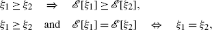
• (c) If ξ ₁≥ξ ₂, then for all 0≤t≤T. In addition, if a.s. for some t∈[0,T], then ξ ₁=ξ ₂.

Proposition 6.2.1 shows that all essential properties of the standard linear conditional expectation, except linearity, are preserved under the notion of an -consistent nonlinear expectation.

From the modelling point of view, we should be able to generate -consistent nonlinear expectations in a feasible way. The next example shows one possible way of generating -consistent nonlinear expectations.

Example 6.1

Choose a continuous, strictly increasing function $\varphi:{\mathbb{R}}\rightarrow {\mathbb{R}}$. The operator

(6.4)

is an -consistent nonlinear expectation. The nonlinear expectation (6.4) can be interpreted as the indifference price of ξ determined by an agent with utility φ, see Royer (2006).

It turns out that -consistent nonlinear expectations can be defined by nonlinear BSDEs. In this chapter we study the BSDEs

(6.5)

By a nonlinear BSDE we mean a BSDE with a nonlinear generator g.

Definition 6.2.3

Consider $g:\varOmega\times[0,T]\times\mathbb{R}\times\mathbb {R}\times L^{2}_{Q}(\mathbb{R})\rightarrow\mathbb{R}$ such that

• (i) g satisfies (A2) from Chap. 3,

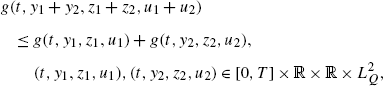
• (ii) g satisfies the inequality

  

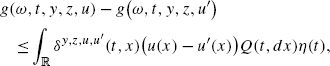
  a.s., a.e. (ω,t)∈Ω×[0,T], for all $(y,z,u),(y,z,u')\in\mathbb{R} \times\mathbb{R}\times L^{2}_{Q}(\mathbb{R})$, where $\delta ^{y,z,u,u'}:\varOmega\times[0,T]\times {\mathbb{R}}\rightarrow(-1,\infty)$ is a predictable process such that the mapping $t\mapsto\int_{\mathbb{R}}|\delta^{y,z,u,u'}(t,x)|^{2}Q(t,dx)\eta(t)$ is uniformly bounded in (y,z,u,u′),

• (iii) g(t,y,0,0)=0 for all $(t,y)\in[0,T]\times {\mathbb{R}}$.

• (a) We define the g-expectation by

  

  where Y(0) is the unique solution to the BSDE (6.5) with the generator g satisfying (i)–(iii) and the terminal condition .

• (b) We define the conditional g-expectation by

  

  where Y(t) is the unique solution to the BSDE (6.5) with the generator g satisfying (i)–(iii) and the terminal condition .

Notice that for the g-expectation its dynamic version is naturally defined.

We state the first key result of this chapter.

Theorem 6.2.1

The g-expectation is an -consistent nonlinear expectation.

Proof

The strict monotonicity of follows from the comparison principle established in Theorem 3.2.2. Since g(t,y,0,0)=0, we can choose Y=c,Z=U=0 as the unique solution to the BSDE (6.5) with ξ=c. Hence, the invariance property of holds. We now prove the -consistency of . Choose t∈[0,T] and . We investigate

where Y and Y′ denote the unique solutions to the BSDEs

Since g(t,y,0,0)=0, we can put Y′(s)=Y(t)1 _A , Z′(s)=U′(s,z)=0, $(s,z)\in[t,T]\times {\mathbb{R}}$. Consequently, we obtain the equations

Consider the BSDE

Since g(t,y,0,0)=0 we can also put Y(s)=Y″(s)1 _A , Z(s)=Z″(s)1 _A , U(s,z)=U″(s,z)1 _A $(s,z)\in [t,T]\times {\mathbb{R}}$. Hence, we end up with the equations

By uniqueness of solutions we finally conclude that Y(s)=Y′(s), Z(s)=Z′(s), U(s,z)=U′(s,z), $(s,z)\in[0,t]\times {\mathbb{R}}$. Hence, is a filtration-consistent expectation with the conditional expectation . □

Any g-expectation clearly satisfies the properties from Proposition 6.2.1, which can now be derived from properties of BSDEs.

Example 6.2

If we consider a BSDE with zero generator, then the g-expectation coincides with the linear conditional expectation. If we consider the BSDE from Proposition 3.3.2 or 3.4.2, then the g-expectation is a filtration-consistent nonlinear expectation.

We are now interested in a converse of Theorem 6.2.1. The first results in this field were proved by Coquet et al. (2002) and Rosazza Gianin (2006) for the Brownian filtration. We present the result proved by Royer (2006) for the filtration generated by a Lévy process. First, we introduce two particular types of g-expectations.

Proposition 6.2.2

Consider the natural filtration generated by a Lévy process with a Lévy measure ν. For α>0 and −1<β≤0 we define the generators

The corresponding g-expectations have the representations

where

and (ϕ,κ) are -predictable processes satisfying

Proof

The result can be derived by following the arguments from Propositions 3.3.2 and 3.4.2, see also Proposition 3.6 in Royer (2006). □

We now state the second key result of this chapter, see Theorem 4.6 in Royer (2006).

Theorem 6.2.2

Consider the natural filtration generated by a Lévy process with a Lévy measure ν. Let be an -consistent nonlinear expectation such that

• (i) for all

  

  where is the g-expectation defined in Proposition 6.2.2,

• (ii) for all and

  

Then, there exists a function $g: \varOmega\times[0,T]\times {\mathbb{R}}\times L^{2}_{Q}\rightarrow {\mathbb{R}}$ and the g-expectation such that

Moreover, the following properties hold:

• (i) g satisfies (A2) from Chap. 3,

• (ii) g satisfies the inequality

  

  a.s., a.e. (ω,t)∈Ω×[0,T], for all $(z,u),(z,u')\in\mathbb{R}\times L^{2}_{Q}(\mathbb{R})$, where $\delta^{z,u,u'}:\varOmega\times[0,T]\times {\mathbb{R}}\rightarrow(-1,\infty )$ is a predictable process such that δ ^z,u,u′(t,x)>−1 and |δ ^z,u,u′(t,x)|≤K(1∧|x|) for all $(t,x,z,u,u')\in [0,T]\times {\mathbb{R}}\times {\mathbb{R}}\times L^{2}_{Q}\times L^{2}_{Q}$,

• (iii) g(t,0,0)=0 for all t∈[0,T],

• (iv) g satisfies the growth conditions

  

  for $(t,z,u)\in[0,T]\times\mathbb{R}\times L^{2}_{Q}(\mathbb{R})$.

The first condition of Theorem 6.2.2 is called the domination condition. We remark that a large class of nonlinear expectations satisfies the domination condition, see Rosazza Gianin (2006) and Royer (2006). The second condition requires translation invariance of the nonlinear expectation with respect to “known” pay-offs, which is a reasonable assumption provided that discounting of pay-offs is not allowed in the valuation, see Sect. 13.1.

The importance of Theorem 6.2.2 is obvious. Theorem 6.2.2 shows that all filtration-consistent nonlinear expectations which satisfy the domination condition and the translation invariance property can be derived from BSDEs. Consequently, when we study “regular” filtration-consistent nonlinear expectations we can focus on g-expectations. Notice that the generator derived under the assumptions of Theorem 6.2.2 depends only on the control processes (Z,U) and is independent of Y. This is the consequence of the assumed translation invariance property for the nonlinear expectation.

It is clear that the generator g of a BSDE plays a crucial role in defining a g-expectation. Some important properties of g-expectations can be related to properties of generators g.

Proposition 6.2.3

Let be a g-expectation.

• (a) If g is independent of y, then is translation invariant

  

• (b) If g is positively homogenous, then is positively homogenous

  

• (c) If g is convex

  

  then is convex

  

• (d) If g is sub-linear: sub-additive

  

  and positively homogenous, then is sub-linear: sub-additive

  

  positively homogenous.

Proof

(a) We deal with two BSDEs

We can easily conclude that Y ^ξ+c(t)=Y ^ξ(t)+c, Z ^ξ+c(t)=Z ^ξ(t), U ^ξ+c(t,z)=U ^ξ(t,z), $(t,z)\in[0,T]\times {\mathbb{R}}$.

(b) We deal with two BSDEs

We can easily conclude that Y ^cξ(t)=cY ^ξ(t), Z ^cξ(t)=cZ ^ξ(t), U ^cξ(t,z)=cU ^ξ(t,z), $(t,z)\in[0,T]\times {\mathbb{R}}$.

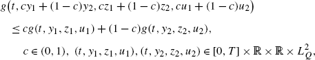
(c) We deal with three BSDEs

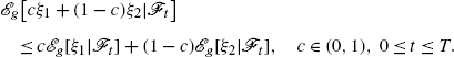
We introduce the processes $Y(t)=c Y^{\xi_{1}}(t)+(1-c)Y^{\xi_{2}}(t)$, $Z(t)=c Z^{\xi_{1}}(t)+(1-c)Z^{\xi_{2}}(t)$, $U(t,z)= U^{\xi _{1}}(t,z)+(1-c)U^{\xi_{2}}(t,z)$. It is straightforward to notice that (Y,Z,U) satisfies the BSDE

(6.6)

Since g satisfies

the BSDE (6.6) can be written as

with a nonnegative function h. By the comparison principle we get $Y^{c\xi_{1}+(1-c)x_{2}}(t)\leq Y(t)=c Y^{\xi_{1}}(t)+(1-c)Y^{\xi_{2}}(t)$, 0≤t≤T.

(d) Adapting the arguments from (b) and (c), we can prove the assertion. □

The properties from Proposition 6.2.3 are used in Chap. 13 where we deal with dynamic risk measures.

Bibliographical Notes

The Choquet expectation was introduced by Choquet (1953). Properties of Choquet expectations and the Wang transform together with their failures in non-Gaussian financial models are discussed by Nguyen et al. (2012). The g-expectations was introduced by Peng (1997). For the connection between the Choquet expectation and the g-expectation we refer to Chen et al. (2005) and Chen and Kulperger (2006). In the proof of Proposition 6.2.3 we follow the arguments from Rosazza Gianin (2006) and Jiang (2008). We refer to Rosazza Gianin (2006) and Jiang (2008) for stronger relations between static and dynamic properties of g-expectations and generators of BSDEs defining the g-expectations. For a representation of a filtration-consistent nonlinear expectation in a general separable space we refer to Cohen (2011). We remark that g-expectations allow for introducing nonlinear versions of some well-known probabilistic results, see Coquet et al. (2002), Peng (1997), Rosazza Gianin (2006) and Royer (2006). For g-martingales, g-submartingales, g-supermartingales and nonlinear Doob-Meyer decomposition we refer to Coquet et al. (2002) and Royer (2006).

References

Chen, Z., Kulperger, R.: Minimax pricing and Choquet expectations. Insur. Math. Econ. 38, 518–528 (2006)
Chen, Z., Chen, T., Davison, M.: Choquet expectation and Peng’s g-expectations. Ann. Probab. 33, 1179–1199 (2005)
Choquet, G.: Theory of capacities. Ann. Inst. Fourier 5, 131–195 (1953)
Cohen, S.N.: Representing filtration consistent non-linear expectations as g-expectations in general probability spaces. Preprint (2011)
Coquet, F., Hu, Y., Mémin, J., Peng, S.: Filtration-consistent non-linear expectations and related g-expectations. Probab. Theory Relat. Fields 123, 1–27 (2002)
Jiang, L.: Convexity, translation invariance and subadditivity for g-expectations and related risk measures. Ann. Appl. Probab. 18, 245–258 (2008)
Nguyen, H., Pham, U., Tran, H.: On some claims related to Choquet integral risk measures. Ann. Oper. Res. 195, 5–31 (2012)
Peng, S.: Backward SDE and related g-expectations. In: El Karoui, N., Mazliak, L. (eds.) Backward Stochastic Differential Equations, Pitman Research Notes, pp. 141–161. Pitman, London (1997)
Rosazza Gianin, E.: Risk measures via g-expectations. Insur. Math. Econ. 39, 19–34 (2006)
Royer, M.: Backward stochastic differential equations with jumps and related non-linear expectations. Stoch. Process. Appl. 116, 1358–1376 (2006)
Wang, S.: A class of distortion operators for pricing financial and insurance risks. J. Risk Insur. 1, 15–36 (2000)
Author information
Authors and Affiliations
Rights and permissions
Copyright information
© 2013 Springer-Verlag London
About this chapter
Cite this chapter
Delong, Ł. (2013). Nonlinear Expectations and g-Expectations. In: Backward Stochastic Differential Equations with Jumps and Their Actuarial and Financial Applications. EAA Series. Springer, London. https://doi.org/10.1007/978-1-4471-5331-3_6
Download citation
DOI: https://doi.org/10.1007/978-1-4471-5331-3_6
Publisher Name: Springer, London
Print ISBN: 978-1-4471-5330-6
Online ISBN: 978-1-4471-5331-3
eBook Packages: Mathematics and StatisticsMathematics and Statistics (R0)