
Abstract
We consider two optimization problems which take into account the uncertainty about the true probability (martingale) measure. First, we investigate pricing and hedging under model ambiguity. We find the hedging strategy which minimizes the expected terminal shortfall under a least favorable probability measure specifying the probability model for the risk factors and we set the price which offsets this worst shortfall. Next, we deal with no-good-deal pricing. We price the insurance payment process with a least favorable martingale measure under a Sharpe ratio constraint which excludes prices leading to extraordinarily high gains. Both pricing and hedging objectives lead to the same solution. We characterize the price and the hedging strategy by a nonlinear BSDE.
Access provided by Autonomous University of Puebla. Download chapter PDF
Keywords
These keywords were added by machine and not by the authors. This process is experimental and the keywords may be updated as the learning algorithm improves.
In this chapter we solve two optimization problems which take into account the uncertainty about the true probability (martingale) measure. We investigate pricing and hedging under model ambiguity and we deal with no-good-deal pricing. Both objectives have strong theoretical and practical justifications. In both cases the goal is to derive a price and a hedging strategy by optimizing the expectation of a pay-off over a set of equivalent probability (martingale) measures. The least favorable measure is found and used for pricing and hedging. The connection between the objectives considered in this chapter and pricing and hedging under the instantaneous mean-variance risk measure considered in Sect. 10.4 is given.
1 Pricing and Hedging Under Model Ambiguity
In previous chapters we assumed that we know the true real-world probability measure (the true probability law) or we know the true parameters of the combined financial and insurance model. In real applications the true probabilities or the true values of parameters are uncertain and we face so-called model ambiguity.
We consider the financial model (7.1)–(7.2) and the insurance payment process (7.3). We assume that the process J is a point process and, consequently, the jump measure N of the point process J has the compensator ϑ(dt,{1})=η(t)dt. We allow for model ambiguity or Knightian uncertainty, see Chen and Epstein (2002). We introduce the set of equivalent probability measures

where ψ, ϕ and κ are predictable processes such that

and L is a predictable process. The purpose of the set  is to represent different beliefs (different assumptions) about the parameters or the probability laws of the risk factors in our model. One way of determining the set
  for ambiguity modelling is to specify confidence sets around the estimates of the parameters and to take for
  the class of all measures that are consistent with these confidence sets. Then, the process L can be interpreted as an estimation error. Alternatively, the elements of
  can be interpreted as prior models which specify probabilities of future scenarios for the risk factors. Then, the process L can define the range of equivalent probabilities for every scenario.
Let us introduce the risk measure

The risk measure (12.2) measures the risk of a financial position ξ. We remark that ξ>0 is interpreted as a profit and ξ<0 as a loss. Under (12.2) we take the supremum of all expected shortfalls for all prior models and we are interested in the expected shortfall under the least favorable model (the least favorable assumptions).
We apply the conditional version of the risk measure (12.2) to the discounted surplus at time T (the net asset value at time T). We investigate the risk measures

where the investment portfolio X
π under an admissible investment strategy  is given by (7.11). The goal is to find an admissible investment strategy π which minimizes the risk measures ρ
t
for all t∈[0,T] and a price Y which makes the risk measures vanish in the sense that
is given by (7.11). The goal is to find an admissible investment strategy π which minimizes the risk measures ρ
t
for all t∈[0,T] and a price Y which makes the risk measures vanish in the sense that

under the condition that X(t)=Y(t). The price and the hedging strategy are given by

The hedging strategy leads to the lowest expected terminal shortfall of the assets below the liabilities under the least favorable probability measure from the set of prior models. The price offsets this expected terminal shortfall. The objective seems to be a sound pricing and hedging objective for insurers who are forced by regulators to carry stress-tests on model parameters and hold sufficient capital to withstand extreme scenarios. By applying the risk measure (12.3) the insurer protects the terminal net asset wealth under the scenario in which the worst model assumptions turn out to be the true assumptions. We remark that (12.3) is an example of robust utility optimization, see Schied (2005) and Schied (2006).
We now solve the optimization problem

We deal with three BSDE:

where  and
and  ,
,

where  , and
, and

By Propositions 3.3.1 and 3.4.1 we can derive the representation

where \({\mathbb{Q}}^{\psi,\phi,\kappa}\) is induced by  .
.
Theorem 12.1.1
Let us assume that (C1)–(C4) from Chap. 7 hold and the jump measure N of the step process J has the compensator ϑ(dt,{1})=η(t)dt. We consider a predictable process L such that L(t)≥θ(t)+ε, ε>0, and L(t)≤K, 0≤t≤T.
-
(a)
There exist unique solutions \((Y^{\pi, \psi,\phi,\kappa },Z_{1}^{\pi, \psi,\phi,\kappa},Z_{2}^{\pi, \psi,\phi,\kappa },U^{\pi, \psi,\phi,\kappa}), (Y^{\pi, *},\allowbreak Z_{1}^{\pi, *},Z_{2}^{\pi , *},U^{\pi,*})\in\mathbb{S}^{2}({\mathbb{R}})\times\mathbb{H}^{2}({\mathbb{R}})\times \mathbb{H}^{2}({\mathbb{R}})\times\mathbb{H}_{N}^{2}({\mathbb{R}})\) to the BSDEs (12.5) and (12.6) with
 and
and
 .
. -
(b)
For any
 and
and
 we have
Y
π,ψ,ϕ,κ(t)≤Y
π,∗(t), 0≤t≤T.
we have
Y
π,ψ,ϕ,κ(t)≤Y
π,∗(t), 0≤t≤T. -
(c)
For any
 such that
we have
 , 0≤t≤T.
 and
and
 .
. and
and
 we have
Y
π,ψ,ϕ,κ(t)≤Y
π,∗(t), 0≤t≤T.
we have
Y
π,ψ,ϕ,κ(t)≤Y
π,∗(t), 0≤t≤T. such that

 , 0≤t≤T.
Proof
(a) Choose  and
and  . By (3.22), (10.46) and Theorem 3.1.1 there exist unique solutions to the BSDEs (12.5) and (12.6).
(b) Notice that the generator f of the BSDE (12.5) satisfies the property

with δ y,z,u,u′(t)=κ(t), for \((t,y,z,u),(t,y,z,u')\in [0,T]\times {\mathbb{R}}\times {\mathbb{R}}\times {\mathbb{R}}\). Recalling the arguments from the proof of Theorem 3.2.2 that led to (3.31), we obtain

where \({\mathbb{Q}}^{\psi,\phi,\kappa}\) is induced by  . It is straightforward to check that the triple

is the solution to the optimization problem

and the global maximum of (12.10) is equal to \(\delta\sqrt {u^{2}+w^{2}+v^{2}\eta}\). Hence, from (12.8)–(12.10) we conclude that Y
π,∗(t)−Y
π,ψ,ϕ,κ(t)≥0 for all t∈[0,T] and any  ,
,  .
.
(c) Recalling (12.9), we define

The assumptions on π guarantee that  . The solution \((Y^{\pi, \psi^{*},\phi^{*}, \kappa^{*}}, Z_{1}^{\pi, \psi^{*},\phi^{*}, \kappa^{*}},Z_{2}^{\pi, \psi^{*},\phi^{*}, \kappa^{*}}, U^{\pi, \psi^{*},\phi^{*}, \kappa ^{*}})\) coincides with \((Y^{\pi,*},\allowbreak Z_{1}^{\pi,*},\allowbreak Z_{2}^{\pi,*},U^{\pi ,*})\) by uniqueness of solution to (12.5). Hence, we conclude that
  for all t∈[0,T] and any
  . Since
  by item (b), the assertion of item (c) can be immediately deduced. □
We remark that the assumption on π from item (c) guarantees that the inequality κ(t)>−1 is strict in the optimum. Without this assumption, the least favorable measure cannot be found in the set  .
.
Theorem 12.1.2
Let us assume that (C1)–(C4) from Chap. 7 hold and the jump measure N of the step process J has the compensator ϑ(dt,{1})=η(t)dt. We consider a predictable process L such that L(t)≥θ(t)+ε, ε>0, and L(t)≤K, 0≤t≤T.
-
(a)
There exist unique solutions \((Y^{\pi, *},Z_{1}^{\pi, *},Z_{2}^{\pi, *},U^{\pi, *}), (Y^{*, *},Z_{1}^{*, *},Z_{2}^{*, *},U^{*, *})\,{\in} \mathbb{S}^{2}({\mathbb{R}})\times\mathbb{H}^{2}({\mathbb{R}})\times\mathbb {H}^{2}({\mathbb{R}})\times\mathbb{H}_{N}^{2}({\mathbb{R}})\) to the BSDEs (12.6) and (12.7) with
 .
. -
(b)
Define the class of admissible strategies
 which consists of strategies
π:=(π(t),0≤t≤T) such that
which consists of strategies
π:=(π(t),0≤t≤T) such that
 and
and
For any
 we have
Y
π,∗(t)≥Y
∗,∗(t), 0≤t≤T.
we have
Y
π,∗(t)≥Y
∗,∗(t), 0≤t≤T. -
(c)
Let Y denote the optimal value function of the optimization problem (12.4) under the new set of admissible strategies
 . If
U
∗,∗(t)≥0 or |L(t)|2<η(t)+|θ(t)|2
on the set {η(t)>0}, 0≤t≤T, then
. If
U
∗,∗(t)≥0 or |L(t)|2<η(t)+|θ(t)|2
on the set {η(t)>0}, 0≤t≤T, then
 , 0≤t≤T, and the optimal admissible hedging strategy
 takes the form
 (12.12)
 .
. which consists of strategies
π:=(π(t),0≤t≤T) such that
which consists of strategies
π:=(π(t),0≤t≤T) such that
 and
and

 we have
Y
π,∗(t)≥Y
∗,∗(t), 0≤t≤T.
we have
Y
π,∗(t)≥Y
∗,∗(t), 0≤t≤T. . If
U
∗,∗(t)≥0 or |L(t)|2<η(t)+|θ(t)|2
on the set {η(t)>0}, 0≤t≤T, then
. If
U
∗,∗(t)≥0 or |L(t)|2<η(t)+|θ(t)|2
on the set {η(t)>0}, 0≤t≤T, then
 , 0≤t≤T, and the optimal admissible hedging strategy
 takes the form

Proof
(a) Choose  . By (3.22), (10.46) and Theorem 3.1.1 there exist unique solutions to the BSDEs (12.6) and (12.7).
(b) We introduce the process

and we get the BSDE

Notice that the generator f of the BSDE (12.14) satisfies the property

where

From the Lipschitz property (10.46) and boundedness of L we deduce that the mapping \(t\mapsto|\delta ^{Y^{*,*},Z_{1}^{*,*},Z_{2}^{*,*},U^{\pi,*},U^{*,*}}(t)|^{2}\eta(t)\) is uniformly bounded. We also have

where

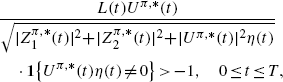
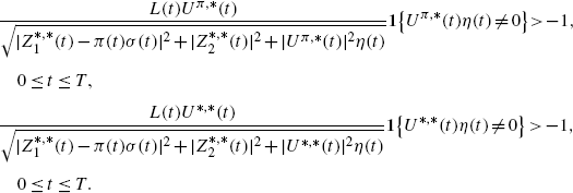
and α
π∈[0,1]. We can conclude that \(\delta ^{Y^{*,*},Z_{1}^{*,*},Z_{2}^{*,*},U^{\pi,*},U^{*,*}}(t)>-1\), 0≤t≤T, for any admissible strategy  . Recalling the arguments from the proof of Theorem 3.2.2 that led to (3.31), we obtain

under some measure \({\mathbb{Q}}\). We now introduce the function

By classical differential calculus we can find the global maximum of φ and we can show that φ(π)≤0. Hence, from (12.15) we conclude that Y
∗,∗(t)−Y
π,∗(t)≤0 for all t∈[0,T] and any  .
.
(c) It is easy to show that φ(π
∗)=0 for π
∗ defined in (12.12). We have to check the admissibility of the candidate strategy π
∗. Predictability and the square integrability of π
∗ are obvious. It is also clear that there exists an adapted, càdlàg solution \(X^{\pi^{*}}\) to (7.11). Hence,  . By uniqueness of solution to (12.14) the solution \((Y^{\pi^{*},*},\hat {Z}_{1}^{\pi^{*},*},Z_{2}^{\pi^{*},*},U^{\pi^{*},*})\) coincides with \((Y^{*,*},Z_{1}^{*,*},Z_{2}^{*,*},U^{*,*})\). From (12.12) we can now derive

and, consequently,  if
if

which holds if U
∗,∗(t)≥0 or |L(t)|2<η(t)+|θ(t)|2 on the set {η(t)>0}. We can conclude that  for all t∈[0,T]. Since
  by item (b), the assertion of item (c) can be deduced. □
The additional constraints on the set of admissible strategies allow us to apply the comparison principle in the proof of Theorem 12.1.2 and we succeed in obtaining the optimal solution. We point out that the additional constraints are essential for deriving the arbitrage-free price (12.4) which satisfies the comparison principle (the property of monotonicity with respect to the claim and the Sharpe ratio).
Notice that the assumptions: θ(t)+ε≤L(t) and |L(t)|2<η(t)+|θ(t)|2 on the set {η(t)>0} may hold only if η(t)≥ε>0 on the set {η(t)>0}. We remark that it is reasonable to assume that there exists a positive lower bound on the claim intensity, e.g. despite improvements in mortality, it is reasonable to assume that there exists a natural limit in these improvements and the mortality intensity process should be bounded away from zero. If \(\theta(t)+\varepsilon \leq L(t)<\sqrt{\eta (t)}\), then  .
.
Theorem 12.1.2 shows that the price process and the optimal hedging strategy, which are derived under the ambiguity risk minimization (12.4), can be characterized with the solution to the nonlinear BSDE (12.7). The price process Y ∗,∗ is arbitrage-free. From (12.7) we get

and by the Girsanov’s theorem we obtain the representation

where the equivalent martingale measure \({\mathbb{Q}}^{*}\) is given by

Since we assume that U ∗,∗(t)≥0 or |L(t)|2<η(t)+|θ(t)|2, the process given by (12.17) is a positive martingale and it defines an equivalent martingale measure. We can also prove that Y ∗,∗ satisfies the comparison principle and the property of monotonicity with respect to the claim, see Delong (2012a). The systematic and unsystematic insurance risks are priced under \({\mathbb{Q}}^{*}\) and the insurance risk premiums can be deduced from (12.17). The pricing measure \({\mathbb{Q}}^{*}\) depends on the financial market, the insurance payment process and the control process L. Since Y ∗,∗ is an arbitrage-free price of the liability and Z ∗,∗ is the control process of the BSDE for Y, we conclude that the optimal hedging strategy (12.12) is a delta hedging strategy with a correction term.
Recall now the hedging strategy (10.43) and the price (10.44) derived under the instantaneous mean-variance risk measure. There are obvious similarities between the results from Sect. 10.4 and the results of this chapter. This should not mislead us. We point out that the price process (10.44), which is obtained under the assumptions of Theorem 10.4.1, may give rise to arbitrage opportunities, see Example 10.3. This is never the case for the price process (12.7), which is obtained under the assumptions of Theorems 12.1.1 and 12.1.2. The stronger assumptions of Theorems 12.1.1 and 12.1.2 exclude those cases of (10.44) which lead to arbitrage prices, see Examples 10.3 and 10.4.
We conclude that there is an equivalence between arbitrage-free pricing and hedging under the instantaneous mean-variance risk measure and pricing and hedging under the ambiguous risk measure, which, by construction, always leads to an arbitrage-free price. Such an equivalence is beneficial for applications and interpretations. Firstly, it is straightforward to justify that L(t)≥θ(t)+ε as the process L can be related to the Sharpe ratio of the surplus process. Secondly, from (10.43) and (10.56) we deduce that the correction term in the hedging strategy (10.43) or (12.12) arises if the insurer applies the mean-variance risk measure instead of the variance risk measure.
Example of pricing and hedging under model ambiguity are given in Examples 10.3 and 10.4.
2 No-Good-Deal Pricing
In the arbitrage-free financial and insurance model the payment process P should be priced by the expectation \({\mathbb{E}}^{\mathbb{Q}}[\int_{0}^{T}e^{-rt}dP(t)]\) under an equivalent martingale measure  , see Sect. 9.1. Since the set of equivalent martingale measures
  is not a singleton, the first idea is to consider
  . Such a superhedging price is too high for practical applications, gives rise to arbitrage opportunities and cannot be used for pricing, see Sect. 9.3. The second idea is to consider
  where
where  . In order to apply such a price, the form of the subset
  of the set of equivalent martingale measures
  should be specified and justified. In this chapter we present a financial motivation for considering a particular subset of
  and we find the arbitrage-free price under the least favorable martingale measure from this subset.
We investigate the insurance payment process (7.3). We assume that the process J is a point process and, consequently, the jump measure N of the point process J has the compensator ϑ(dt,{1})=η(t)dt. From Propositions 3.3.1 and 3.4.1 we can conclude that an arbitrage-free price Y of the payment process P must satisfy the BSDE

where ϕ and κ denote the insurance risk premiums and  . We aim to constrain the possible values of
  in a financially sensible way. A reasonable constraint on the risk premiums can be derived by referring to the theory of no-good-deal pricing.
Sharpe ratios are often used to characterize investment opportunities. An investment opportunity with an extraordinarily high Sharpe ratio is called a good deal and the theory of finance argues that good deals cannot survive in competitive markets, see Cochrane and Saá-Requejo (2000) and Björk and Slinko (2006). Empirical studies also support the fact that Sharpe ratios of investment opportunities in competitive markets take restricted range of values, see Lo (2002). These arguments lay the foundation for no-good-deal pricing.
We assume that the stock and the insurance contract are traded in the market. We remark that market-consistent valuation of insurance liabilities assumes that insurance obligations can be transferred between parties, see V.2.–V.3. in European Commission QIS5 (2010). The insurer has two risky opportunities: he can invest in the risky stock or he can sell the risky insurance payment process, collect a premium and back the liability with the risk-free investment in the bank account. We define the instantaneous Sharpe ratios of the investment in the stock S and the investment in the insurance contract Y:

where we use the Sharpe ratio of the surplus  which is earned by the insurer who takes the short position in the insurance contract and the long position in the bank account, see (10.41) and (10.42). By the Schwarz inequality we get

which yields the inequality

The goal is to find a least favorable martingale measure for pricing the insurance payment process under the constraint that the Sharpe ratio of the insurance contract is within the no-good-deal range given by the market. In order to guarantee that in the combined financial and insurance market the instantaneous Sharpe ratios are bounded by a process L, which itself should be bounded to exclude good deals, we have to introduce the constraint

The bound L for the Sharpe ratio of the insurance contract should be greater than θ since the risk premium θ can be earned by investing in the stock. The insurance contract carries an additional risk and the risk premium for the insurance contract has to be strictly above θ. Hence, we should consider L(t)≥θ(t)+ε, ε>0.
We now define the no-good-deal price of the insurance payment process P. We choose a process L which represents the bound on possible gains in the market measured by instantaneous Sharpe ratios. We introduce the set of equivalent martingale measures

where ϕ and κ are predictable processes such that

The no-good-deal price is defined by

We price the insurance payment process with a least favorable martingale measure under the Sharpe ratio constraint which excludes too good prices leading to extraordinarily high gains. The constraint (12.20) has a financial justification and leads to the well-defined optimization problem (12.22).
Following the steps from the proofs of Theorems 12.1.1 and 12.1.2, we can derive the no-good-deal price.
Theorem 12.2.1
Let us assume that (C1)–(C4) from Chap. 7 hold and the jump measure N of the step process J has the compensator ϑ(dt,{1})=η(t)dt. We consider a predictable process L such that L(t)≥θ(t)+ε, ε>0, and L(t)≤K, 0≤t≤T. Let us investigate the BSDE

If U(t)≥0 or |L(t)|2<η(t)+|θ(t)|2 on the set {η(t)>0}, 0≤t≤T, then the no-good-deal price process (12.22) is the unique solution to the BSDE (12.23). The no-good-deal price process has the representation

where the least favorable martingale measure \({\mathbb{Q}}^{*}\) is given by

The no-good-deal price (12.23) coincides with the price (12.7) derived in Theorem 12.1.2 under the ambiguity risk minimization.
Bibliographical Notes
This chapter presents the results from Delong (2012a). Model ambiguity and Knightian uncertainty were introduced by Chen and Epstein (2002) to financial modelling. Risk measures based on least favorable probability measures and robust optimization problems are studied in Leitner (2007), Becherer (2009), Schied (2005), Schied (2006) and McNeil et al. (2005). Becherer (2009) found the hedging strategy which minimizes the expected terminal shortfall under a least favorable probability measure and solved the no-good-deal pricing problem in a diffusion model by applying BSDEs. We use the arguments from Becherer (2009) and we solve the pricing and hedging problems in the model with jumps. Cochrane and Saá-Requejo (2000) introduced the theory of no-good-deal pricing into the financial literature, and Björk and Slinko (2006) were the first to investigate a Lévy-driven asset model. Robust pricing and no-good-deal pricing in insurance is also investigated by Pelsser (2011). Utility maximization and optimal investment and consumption problems under model ambiguity in a jump-diffusion financial market consisting of assets modelled with Itô-Lévy processes are studied by Øksendal and Sulem (2011), Øksendal and Sulem (2012) and Laeven and Stadje (2012). We remark that the min-max problem (12.4) is an example of a stochastic differential game in which two players choose strategies, the first player wishes to minimize a pay-off and the second player wishes to maximize the same pay-off. Stochastic differential games and related BSDEs are considered in Hamadène and Lepeltier (1995), El Karoui and Hamadène (2003), Øksendal and Sulem (2011), Øksendal and Sulem (2012).
References
Becherer, D.: From bounds on optimal growth towards a theory of good-deal hedging. In: Albecher, H., Runggaldier, W., Schachermayer, W. (eds.) Advanced Financial Modelling, pp. 27–52. de Gruyter, Berlin (2009)
Björk, T., Slinko, I.: Towards a general theory of good deal bounds. Rev. Finance 10, 221–260 (2006)
Chen, Z., Epstein, L.: Ambiguity, risk and asset returns in continuous time. Econometrica 70, 1403–1443 (2002)
Cochrane, J., Saá-Requejo, J.: Beyond arbitrage: good-deal asset price bounds in incomplete markets. J. Polit. Econ. 1008, 79–119 (2000)
Delong, Ł.: No-good-deal, local mean-variance and ambiguity risk pricing and hedging for an insurance payment process. ASTIN Bull. 42, 203–232 (2012a)
El Karoui, N., Hamadène, S.: BSDEs and risk-sensitive control, zero-sum and nonzero-sum game problems of stochastic functional differential equations. Stoch. Process. Appl. 107, 145–169 (2003)
European Commission: Fifth quantitative impact study: call for advice and technical specifications. http://ec.europa.eu/internal_market/insurance/solvency/index_en.htm (2010)
Hamadène, S., Lepeltier, J.P.: Zero-sum stochastic differential games and backward equations. Syst. Control Lett. 24, 259–263 (1995)
Laeven, R.J.A., Stadje, M.: Robust portfolio choice and indifference valuation. Preprint (2012)
Leitner, J.: Pricing and hedging with globally and instantaneously vanishing risk. Stat. Decis. 25, 311–332 (2007)
Lo, A.W.: The statistics of Sharpe ratios. Financ. Anal. J. 58, 36–52 (2002)
McNeil, A.J., Frey, R., Embrechts, P.: Quantitative Risk Management. Princeton University Press, Princeton (2005)
Øksendal, B., Sulem, A.: Portfolio optimization under model uncertainty and BSDE games. Quant. Finance 11, 1665–1674 (2011)
Øksendal, B., Sulem, A.: Forward-backward SDE games and stochastic control under model with uncertainty. J. Optim. Theory Appl. (2012, in print)
Pelsser, A.: Pricing in incomplete markets. Preprint (2011)
Schied, A.: Optimal investments for robust utility functionals in complete market models. Math. Oper. Res. 30, 750–764 (2005)
Schied, A.: Risk Measures and Robust Optimization Problems. Lecture Notes (2006). http://people.orie.cornell.edu/~schied/PueblaNotes8.pdf
Author information
Authors and Affiliations
Rights and permissions
Copyright information
© 2013 Springer-Verlag London
About this chapter
Cite this chapter
Delong, Ł. (2013). Pricing and Hedging Under a Least Favorable Measure. In: Backward Stochastic Differential Equations with Jumps and Their Actuarial and Financial Applications. EAA Series. Springer, London. https://doi.org/10.1007/978-1-4471-5331-3_12
Download citation
DOI: https://doi.org/10.1007/978-1-4471-5331-3_12
Publisher Name: Springer, London
Print ISBN: 978-1-4471-5330-6
Online ISBN: 978-1-4471-5331-3
eBook Packages: Mathematics and StatisticsMathematics and Statistics (R0)