Modular Forms for SL₂(ℤ)

Abstract

The notion of a modular form is introduced. The dimension of the space of modular forms is determined and Fourier-expansions of Eisenstein series are determined leading to the first number theoretical applications. The Fourier-coefficients of a modular form are fed into a Dirichlet series thus forming the associated L-function, which is shown to extend to an entire function. Hecke operators acting on modular forms are introduced and it is shown that L-functions of Hecke eigenforms admit Euler products. Finally, non-holomorphic Eisenstein series and Maaß-wave forms, the real-analytic counterparts of modular forms, and there L-functions, are introduced.

These keywords were added by machine and not by the authors. This process is experimental and the keywords may be updated as the learning algorithm improves.

In this chapter we introduce the notion of a modular form and its L-function. We determine the space of modular forms by giving an explicit basis. We define Hecke operators and we show that the L-function of a Hecke eigenform admits an Euler product.

2.1 The Modular Group

Recall the notion of an action of a group G on a set X. This is a map G×X→X, written (g,x)↦gx, such that 1x=x and g(hx)=(gh)x, where x∈X and g,h∈G are arbitrary elements and 1 is the neutral element of the group G.

Two points x,y∈X are called conjugate modulo G, if there exists a g∈G with y=gx. The orbit of a point x∈X is the set Gx of all gx, where g∈G, so the orbit is the set of all points conjugate to x. We write G∖X or X/G for the set of all G-orbits.

Example 2.1.1

Let G be the group of all complex numbers of absolute value one, also known as the circle group

$$G=\mathbb{T}=\bigl\{ z\in\mathbb{C}:|z|=1\bigr\}. $$

The group G acts on the set ℂ by multiplication. The map

is a bijection.

An action of a group is said to be transitive if there is only one orbit, i.e. if any two elements are conjugate.

This is the usual notion of a group action from the left, or left action. Later, in Lemma 2.2.2, we shall also define a group action from the right.

For given g∈G the map x↦gx is invertible, as its inverse is x↦g ⁻¹ x.

The group $\operatorname{GL}_{2}(\mathbb{C})$ acts on the set ℂ²∖{0} by matrix multiplication. Since this action is by linear maps, the group also acts on the projective space ℙ¹(ℂ), which we define as the set of all one-dimensional subspaces of the vector space ℂ². Every non-zero vector in ℂ² spans such a vector space and two vectors give the same space if and only if one is a multiple of the other, which means that they are in the same ℂ^×-orbit. So we have a canonical bijection

$$\mathbb{P}^1(\mathbb{C})\cong\bigl(\mathbb{C}^2 \smallsetminus \{ 0\} \bigr) /\mathbb{C}^\times. $$

We write the elements of ℙ¹(ℂ) in the form [z,w], where (z,w)∈ℂ²∖{0} and

$$[z,w]=\bigl[z',w'\bigr]\quad \Leftrightarrow\quad \exists \lambda\in\mathbb{C}^\times: \bigl(z',w' \bigr)=(\lambda z,\lambda w). $$

For w≠0 there exists exactly one representative of the form [z,1], and the map z↦[z,1] is an injection ℂ↪ℙ¹(ℂ), so that we can view ℂ as a subset of ℙ¹(ℂ). The complement of ℂ in ℙ¹(ℂ) is a single point ∞=[1,0], so that ℙ¹(ℂ) is the one-point compactification $\widehat{\mathbb{C}}$ of ℂ, the Riemann sphere. We consider the action of $\operatorname{GL}_{2}(\mathbb{C})$ given by g.(z,w)=(z,w)g ^t; then with we have

$$g.[z,1] = [az+b,cz+d] = \biggl[\frac{az+b}{cz+d},1 \biggr], $$

if cz+d≠0. The rational function $\frac{az+b}{cz+d}$ has exactly one pole in the set $\widehat{\mathbb{C}}$, so we define an action of $\operatorname{GL}_{2}(\mathbb{C})$ on the Riemann sphere by

if z∈ℂ. Note that cz+d and az+b cannot both be zero (Exercise 2.1). We finalize the definition of this action with

Any matrix of the form with λ≠0 acts trivially, so it suffices to consider the action on the subgroup $\mathrm{SL}_{2}(\mathbb{C})=\{g\in\operatorname{GL}_{2}(\mathbb {C}):\det(g)=1\}$.

Lemma 2.1.2

The group SL₂(ℂ) acts transitively on the Riemann sphere $\widehat {\mathbb{C}}$. The element acts trivially. If we restrict the action to the subgroup G=SL₂(ℝ), the set $\widehat{\mathbb{C}}$ decomposes into three orbits: ℍ and −ℍ, as well as the set $\widehat{\mathbb{R}}=\mathbb{R}\cup\{\infty\}$.

Proof

For given z∈ℂ one has , so the action is transitive. In particular it follows that $\widehat{\mathbb{R}}$ lies in the G-orbit of the point ∞.

For and z∈ℂ one computes

$$\operatorname{Im}(g.z) = \frac{\operatorname{Im}(z)}{|cz+d|^2}. $$

This implies that G leaves the three sets mentioned invariant. We have and , therefore $\widehat{\mathbb{R}}$ is one G-orbit. We show that G acts transitively on ℍ. For a given z=x+iy∈ℍ one has

$$z = \left ( \begin{array}{c@{\quad }c}\sqrt{y} & \frac{x}{\sqrt{y}} \\ \noalign{\vspace{3pt}} 0 & \frac{1}{\sqrt{y}} \end{array} \right )i. $$

 □

Definition 2.1.3

We denote by LATT the set of all lattices in ℂ. Let $\operatorname{BAS}$ be the set of all ℝ-bases of ℂ, i.e. the set of all pairs (z,w)∈ℂ², which are linearly independent over ℝ. Let $\operatorname{BAS}^{+}$ be the subset of all bases that are clockwise-oriented, i.e. the set of all $(z,w)\in\operatorname{BAS}$ with $\operatorname {Im}(z/w)>0$. There is a natural map

$$\varPsi: \operatorname{BAS}^+ \to \mathrm{LATT}, $$

defined by

$$\varPsi(z,w) = \mathbb{Z}z\oplus\mathbb{Z}w. $$

This map is surjective but not injective, since for example Ψ(z+w,w)=Ψ(z,w). The group Γ ₀=SL₂(ℤ) acts on $\operatorname{BAS}^{+}$ by γ.(z,w)=(z,w)γ ^t=(az+bw,cz+dw) if . Here we remind the reader that an invertible real matrix preserves the orientation of a basis if and only if the determinant of the matrix is positive.

The group Γ ₀=SL₂(ℤ) is called the modular group.

Lemma 2.1.4

Two bases are mapped to the same lattice under Ψ if and only if they lie in the same Γ ₀-orbit. So Ψ induces a bijection

$$\varPsi:\varGamma_0\backslash \operatorname{BAS}^+\stackrel{\cong }{\rightarrow}\mathrm{LATT}. $$

Proof

Let (z,w) and (z′,w′) be two clockwise-oriented bases such that Ψ(z,w)=Λ=Ψ(z′,w′). Since z′,w′ are elements of the lattice generated by z and w, there are a,b,c,d∈ℤ with . Since, on the other hand, z and w lie in the lattice generated by z′ and w′, there are α,β,γ,δ∈ℤ with , so . As z and w are linearly independent over ℝ, it follows that and so is an element of $\operatorname{GL}_{2}(\mathbb{Z})$. In particular one gets det(g)=±1. Since g maps the clockwise-oriented basis (z,w) to the clockwise-oriented basis (z′,w′), one concludes det(g)>0, i.e. det(g)=1 and so g∈Γ ₀, which means that the two bases are in the same Γ ₀-orbit. The converse direction is trivial. □

The set $\operatorname{BAS}^{+}$ is a bit unwieldy, so one divides out the action of the group ℂ^×. This action of ℂ^× on the set $\operatorname{BAS}^{+}$ is defined by ξ(a,b)=(ξa,ξb). One has (a,b)=b(a/b,1), so every ℂ^×-orbit contains exactly one element of the form (z,1) with z∈ℍ. The action of ℂ^× commutes with the action of Γ ₀, so ℂ^× acts on $\varGamma_{0}\backslash \operatorname{BAS}^{+}$. On the other hand, ℂ^× acts on LATT by multiplication and the map Ψ translates one action into the other, which means Ψ(λ(z,w))=λΨ(z,w). As Ψ is bijective, the two ℂ^×-actions are isomorphic and Ψ maps orbits bijectively to orbits, so giving a bijection

$$\varPsi: \varGamma_0\backslash \operatorname{BAS}^+/ \mathbb{C}^\times \stackrel{\cong}{\rightarrow} \mathrm{LATT}/\mathbb{C}^\times. $$

Now let z∈ℍ. Then $(z,1)\in\operatorname{BAS}^{+}$. For one has, modulo the ℂ^×-action:

$$(z,1)\gamma^t\mathbb{C}^\times= (az+b,cz+d) \mathbb{C}^\times= \biggl(\frac{az+b}{cz+d},1\biggr) \mathbb{C}^\times. $$

Letting Γ ₀ act on ℍ by linear fractionals, the map z↦(z,1)ℂ^× is thus equivariant with respect to the actions of Γ ₀.

Theorem 2.1.5

The map z↦ℤz+ℤ induces a bijection

$$\varGamma_0\backslash \mathbb{H}\stackrel{\cong}{\rightarrow} \mathrm {LATT}/ \mathbb{C}^\times. $$

Proof

The map is a composition of the maps

$$\varGamma_0\backslash \mathbb{H}\stackrel{\varphi }{\rightarrow} \varGamma_0\backslash \operatorname{BAS}^+/\mathbb{C}^\times \stackrel{\cong}{\rightarrow} \mathrm{LATT}/\mathbb{C}^\times, $$

so it is well defined. We have to show that φ is bijective.

To show surjectivity, let $(v,w)\in\operatorname{BAS}^{+}$. Then (v,w)ℂ^×=(v/w,1)ℂ^× and v/w∈ℍ, so φ is surjective. For injectivity, assume φ(Γ ₀ z)=φ(Γ ₀ w). This means Γ ₀(z,1)ℂ^×=Γ ₀(w,1)ℂ^×, so there are and λ∈ℂ^× with (w,1)=γ(z,1)λ. The right-hand side is

$$\gamma(z,1)\lambda= \lambda(az+b,cz+d) = (w,1). $$

Comparing the second coordinates, we get λ=(cz+d)⁻¹ and so $w=\frac{az+b}{cz+d}=\gamma.z$, as claimed. □

The element acts trivially on the upper half plane ℍ. This motivates the following definition.

Definition 2.1.6

Let $\overline{\varGamma }_{0}=\varGamma_{0}/\pm1$. For a subgroup Γ of Γ ₀ let $\overline{\varGamma }$ be the image of Γ in $\overline{\varGamma }_{0}$. Then we have

Let

$$S\stackrel{\mathrm{def}}{=}\left(\matrix{0& {-1}\cr1& 0}\right),\qquad T\stackrel{\mathrm{def}}{=}\left(\matrix{1&1\cr0&1}\right). $$

One has

$$Sz = \frac{-1}{z},\qquad Tz=z+1, $$

as well as S ²=−1=(ST)³. Denote by D the set of all z∈ℍ with $|\operatorname{Re}(z)|<\frac{1}{2}$ and |z|>1, as depicted in the next figure. Let $\overline{D}$ be the closure of D in ℍ. The set D is a so-called fundamental domain for the group SL₂(ℤ); see Definition 2.5.17.

Theorem 2.1.7

• (a) For every z∈ℍ there exists a γ∈Γ ₀ with $\gamma z\in\overline{D}$.

• (b) If $z,w\in\overline{D}$, with z≠w, lie in the same Γ ₀-orbit, then we have $\operatorname{Re}(z)=\pm\frac{1}{2}$ and z=w±1, or |z|=1 and w=−1/z. In any case the two points lie on the boundary of D.

• (c) For z∈ℍ let Γ _0,z be the stabilizer of z in Γ ₀. For $z\in\overline{D}$ we have Γ _0,z ={±1} except when

  • z=i, then Γ _0,z is a group of order four, generated by S,

  • z=ρ=e ^2πi/3, then Γ _0,z is of order six, generated by ST,

  • $z=-\overline{\rho}=e^{\pi i/3}$, then Γ _0,z is of order six, generated by TS.

• (d) The group Γ ₀ is generated by S and T.

Proof

Let Γ′ be the subgroup of Γ ₀ generated by S and T. We show that for every z∈ℍ there is a γ′∈Γ′ with $\gamma'z\in\overline{D}$. So let in Γ′. For z∈ℍ one has

$$\operatorname{Im}(gz) = \frac{\operatorname{Im}(z)}{|cz+d|^2}. $$

Since c and d are integers, for every M>0 the set of all pairs (c,d) with |cz+d|<M is finite. Therefore there exists γ∈Γ′ such that $\operatorname {Im}(\gamma z)$ is maximal. Choose an integer n such that T ⁿ γz has real part in [−1/2,1/2]. We claim that the element w=T ⁿ γz lies in $\overline{D}$. It suffices to show that |w|≥1. Assuming |w|<1, we conclude that the element −1/w=Sw has imaginary part strictly bigger than $\operatorname {Im}(w)$, which contradicts our choices. So indeed we get w=T ⁿ γz in $\overline{D}$ and part (a) is proven.

We now show parts (b) and (c). Let $z\in\overline{D}$ and let with $\gamma z\in\nobreak \overline{D}$. Replacing the pair (z,γ) by (γz,γ ⁻¹), if necessary, we assume $\operatorname{Im}(\gamma z)\ge\operatorname{Im}(z)$, so |cz+d|≤1. This cannot hold for |c|≥2, so we have the cases c=0,1,−1.

• If c=0, then d=±1 and we can assume d=1. Then γz=z+b and b≠0. Since the real parts of both numbers lie in [−1/2,1/2], it follows that b=±1 and $\operatorname{Re}(z)=\pm1/2$.

• If c=1, then the assertion |z+d|≤1 implies d=0, except if $z=\rho, -\overline{\rho}$, in which case we can also have d=1,−1.

  • If d=0, then |z|=1 and ad−bc=1 implies b=−1, so gz=a−1/z and we conclude a=0, except if $\operatorname{Re}(z)=\pm \frac{1}{2}$, so $z=\rho,-\overline{\rho}$.

  • If z=ρ and d=1, then a−b=1 and gρ=a−1/(1+ρ)=a+ρ, so a=0,1. The case $z=-\overline{\rho}$ is treated similarly.

• If c=−1, one can replace the whole matrix with its negative and thus can apply the case c=1.

Finally, we must show that Γ ₀=Γ′. For this let γ∈Γ ₀ and z∈D. Then there is γ′∈Γ′ with γ′γz=z, so γ=γ′⁻¹∈Γ′. □

2.2 Modular Forms

In this section we introduce the protagonists of this chapter. Before that, we start with weakly modular functions.

Definition 2.2.1

Let k∈ℤ. A meromorphic function f on the upper half plane ℍ is called weakly modular of weight k if

$$f\biggl(\frac{az+b}{cz+d}\biggr) = (cz+d)^{k}f(z) $$

holds for every z∈ℍ, in which f is defined and every .

Note: for such a function f≠0 to exist, k must be even, since the matrix lies in SL₂(ℤ).

For we denote the induced map $z\mapsto\sigma z=\frac{az+b}{cz+d}$ again by σ. Then

$$\frac{d(\sigma z)}{dz} = \frac{1}{(cz+d)^2}. $$

We deduce from this that a holomorphic function f is weakly modular of weight 2 if and only if the differential form ω=f(z) dz on ℍ is invariant under Γ ₀, i.e. if γ ^∗ ω=ω holds for every γ∈Γ ₀, where γ ^∗ ω is the pullback of the form ω under the map γ:ℍ→ℍ.

More generally, we define for k∈ℤ and f:ℍ→ℂ:

$$f|_{k}\sigma (z)\stackrel{\mathrm{def}}{=}(cz+d)^{-k}f \biggl(\frac{az+b}{cz+d}\biggr), $$

where . If k is fixed, we occasionally leave the index out, i.e. we write f|σ=f| _k σ.

Lemma 2.2.2

The maps f↦f|σ define a linear (right-)action of the group G on the space of functions f:ℍ→ℂ, i.e.

• for every σ∈G the map f↦f|σ is linear,

• one has f|1=f and f|(σσ′)=(f|σ)|σ′ for all σ,σ′∈G.

Every right-action can be made into a left-action by inversion, i.e. one defines σf=f|σ ⁻¹ and one then gets (σσ′)f=σ(σ′f).

Proof

The only non-trivial assertion is f|(σσ′)=(f|σ)|σ′. For k=0 this is simply:

$$f|\bigl(\sigma \sigma'\bigr) (z)=f\bigl(\sigma \sigma'z\bigr)=f|\sigma \bigl(\sigma'z\bigr)=(f|\sigma)|\sigma'(z). $$

Let j(σ,z)=(cz+d). One verifies that this ‘factor of automorphy’ satisfies a so-called cocycle relation:

$$j\bigl(\sigma \sigma',z\bigr) = j\bigl(\sigma , \sigma'z\bigr)j\bigl(\sigma',z\bigr). $$

As f| _k σ(z)=j(σ,z)^−k f|₀ σ(z), we conclude

 □

Lemma 2.2.3

Let k∈2ℤ. A meromorphic function f on ℍ is weakly modular of weight k if and only if for every z∈ℍ one has

$$f(z+1)=f(z)\quad\mathit{and}\quad f(-1/z)=z^{k}f(z). $$

Proof

By definition, f is weakly modular if and only if f| _k γ=f for every γ∈Γ ₀, which means that f is invariant under the group action of Γ ₀. It suffices to check invariance on the two generators S and T of the group. □

We now give the definition of a modular function. Let f be a weakly modular function. The map q:z↦e ^2πiz maps the upper half plane surjectively onto the pointed unit disk $\mathbb{D}^{*}=\{z\in\mathbb{C}:0<|z|<1\}$. Two points z,w in ℍ have the same image under q if and only if there is m∈ℤ such that w=z+m. So q induces a bijection $q:\mathbb{Z}\backslash \mathbb{H}\to \mathbb{D}^{*}$. In particular, for every weakly modular function f on ℍ there is a function $\tilde{f}$ on $\mathbb {D}^{*}\smallsetminus q(\{\mbox {poles}\})$ with

$$f(z) = \tilde{f}\bigl(q(z)\bigr). $$

This means that for $w\in\mathbb{D}^{*}$ we have

$$\tilde{f}(w) = f\biggl(\frac{\log w}{2\pi i}\biggr), $$

where logw is an arbitrary branch of the holomorphic logarithm, being defined in a neighborhood of w. Then $\tilde{f}$ is a meromorphic function on the pointed unit disk.

Definition 2.2.4

A weakly modular function f of weight k is called a modular function of weight k if the induced function $\tilde{f}$ is meromorphic on the entire unit disk $\mathbb{D}=\{z\in\mathbb{C}:|z|<1\}$.

Suggestively, in this case one also says that f is ‘meromorphic at infinity’. This means that $\tilde{f}(q)$ has at most a pole at q=0. It follows that poles of $\tilde{f}$ in $\mathbb{D}^{*}$ cannot accumulate at q=0, because that would imply an essential singularity at q=0. For the function f it means that there exists a bound T=T _f >0 such that f has no poles in the region $\{ z\in\mathbb{H}: \operatorname {Im}(z)>T\}$.

The Fourier expansion of the function f is of particular importance. Next we show that the Fourier series converges uniformly. In the next lemma we write C ^∞(ℝ/ℤ) for the set of all infinitely often differentiable functions g:ℝ→ℂ, which are periodic of period 1, which means that one has g(x+1)=g(x) for every x∈ℝ.

Definition 2.2.5

Let D⊂ℝ be an unbounded subset. A function f:D→ℂ is said to be rapidly decreasing if for every N∈ℕ the function x ^N f(x) is bounded on D.

For D=ℕ one gets the special case of a rapidly decreasing sequence.

Examples 2.2.6

• For D=ℕ the sequence $a_{k}=\frac{1}{k!}$ is rapidly decreasing.

• For D=[0,∞) the function f(x)=e ^−x is rapidly decreasing.

• For D=ℝ the function $f(x)=e^{-x^{2}}$ is rapidly decreasing.

Proposition 2.2.7

(Fourier series)

If g is in C ^∞(ℝ/ℤ), then for every x∈ℝ one has

$$g(x) = \sum_{k\in\mathbb{Z}}c_k(g)e^{2\pi ikx}, $$

where $c_{k}(g)=\int_{0}^{1}g(t) e^{-2\pi ikt}\,dt$ and the sum converges uniformly. The Fourier coefficients c _k =c _k (g) are rapidly decreasing as functions in k∈ℤ.

The Fourier coefficients c _k (g) are uniquely determined in the following sense: Let (a _k ) _k∈ℤ be a family of complex numbers such that for every x∈ℝ the identity

$$g(x) = \sum_{k=-\infty}^\infty a_k e^{2\pi i kx} $$

holds with locally uniform convergence of the series. Then it follows that a _k =c _k (g) for every k∈ℤ.

Proof

Using integration by parts repeatedly, we get for k≠0,

So the sequence (c _k (g)) is rapidly decreasing. Consequently, the sum ∑ _k∈ℤ|c _k (g)| converges, so the series ∑ _k∈ℤ c _k (g)e ^2πikx converges uniformly. We only have to show that it converges to g. It suffices to do that at the point x=0, since, assuming we have this convergence at x=0, we can set g _x (t)=g(x+t) and we see

$$g(x) = g_x(0) = \sum_kc_k(g_x). $$

By $c_{k}(g_{x})=\int_{0}^{1}g(t+x)e^{-2\pi ikt}\,dt = e^{2\pi ikx}c_{k}(g)$ we get the claim. So we only have to show g(0)=∑ _k c _k (g). Replacing g(x) with g(x)−g(0), we can assume g(0)=0, in which case we have to show that ∑ _k c _k (g)=0. Let

$$h(x) = \frac{g(x)}{e^{2\pi ix}-1}. $$

As g(0)=0, it follows that h∈C ^∞(ℝ/ℤ) and we have

$$c_k(g) = \int_0^1h(x) \bigl(e^{2\pi i x}-1\bigr)e^{-2\pi ikx}\,dx = c_{k-1}(h)-c_k(h). $$

Since h∈C ^∞(ℝ/ℤ), the series ∑ _k c _k (h) converges absolutely as well and ∑ _k c _k (g)=∑ _k (c _k−1(h)−c _k (h))=0.

Now for the uniqueness of the Fourier coefficients. Let (a _k ) _k∈ℤ be as in the proposition. By locally uniform convergence the following interchange of integration and summation is justified. For l∈ℤ we have

One has

This implies c _l (g)=a _l . □

This nice proof of the convergence of Fourier series is, to the author’s knowledge, due to H. Jacquet.

Let f be a weakly modular function of weight k. As f(z)=f(z+1) and f is infinitely differentiable (except at the poles), one can write it as a Fourier series:

$$f(x+iy) = \sum_{n=-\infty}^{+\infty}c_n(y)e^{2\pi inx}, $$

if there is no pole of f on the line $\operatorname{Im}(w)=y$, which holds true for all but countably many values of y>0. For such y the sequence (c _n (y)) _n∈ℤ is rapidly decreasing.

Lemma 2.2.8

Let f be a modular function on the upper half plane ℍ and let T>0 such that f has no poles in the set $\{\operatorname{Im}(z)>T\}$. For every n∈ℤ and y>T one has c _n (y)=a _n e ^−2πny for a constant a _n . Then

$$f(z) = \sum_{n=-N}^{+\infty}a_ne^{2\pi inz}, $$

where −N is the pole-order of the induced meromorphic function $\tilde{f}$ at q=0. For every y>0, the sequence a _n e ^−yn is rapidly decreasing.

Proof

The induced function $\tilde{f}$ with $f(z)=\tilde{f}(q(z))$ or $\tilde{f}(q)=f(\frac{\log q}{2\pi i})$ is meromorphic around q=0. In a pointed neighborhood of zero, the function $\tilde{f}$ therefore has a Laurent expansion

$$\tilde{f}(w) = \sum_{n=-\infty}^\infty a_n w^n. $$

Replacing w by q(z), one gets

$$f(z) = \sum_{n=-\infty}^{+\infty}a_ne^{2\pi inz}. $$

The claim follows from the uniqueness of the Fourier coefficients. □

Note, in particular, that the Fourier expansion of a modular function f equals the Laurent expansion of the induced function $\tilde{f}$.

Definition 2.2.9

A modular function f is called a modular form if it is holomorphic in the upper half plane ℍ and holomorphic at ∞, i.e. a _n =0 holds for every n<0.

A modular form f is called cusp form if additionally a ₀=0. In that case one says that f vanishes at ∞.

As an example, consider Eisenstein series G _k for k≥4. Write q=e ^2πiz.

Proposition 2.2.10

For even k≥4 we have

$$G_{k}(z) = 2\zeta(k)+2\frac{(2\pi i)^{k}}{(k-1)!}\sum _{n=1}^\infty \sigma_{k-1}(n)q^n, $$

where σ _k (n)=∑ _d|n d ^k is the kth divisor sum.

Proof

On the one hand we have the partial fraction expansion of the cotangent function

$$\pi\cot(\pi z) = \frac{1}{z}+\sum_{m=1}^\infty \biggl(\frac{1}{z+m}+\frac{1}{z-m}\biggr), $$

and on the other

$$\pi\cot(\pi z) = \pi\frac{\cos(\pi z)}{\sin(\pi z)} = i\pi\frac {q+1}{q-1} = \pi i- \frac{2\pi i}{1-q} = \pi i-2\pi i\sum_{n=0}^\infty q^n. $$

So

$$\frac{1}{z}+\sum_{m=1}^\infty\biggl( \frac{1}{z+m}+\frac{1}{z-m}\biggr) = \pi i-2\pi i\sum_{n=0}^\infty q^n. $$

We repeatedly differentiate both sides to get for k≥4,

$$\sum_{m\in\mathbb{Z}}\frac{1}{(z+m)^k} = \frac{1}{(k-1)!}(- 2\pi i)^k\sum_{n=1}^\infty n^{k-1}q^n. $$

The Eisenstein series is

The proposition is proven. □

Let f be a modular function of weight k. For γ∈Γ ₀ the formula f(γz)=(cz+d)^k f(z) shows that the orders of vanishing of f at the points z and γz agree. So the order $\operatorname{ord}_{z} f$ depends only on the image of z in Γ ₀∖ℍ.

We further define $\operatorname{ord}_{\infty}(f)$ as the order of vanishing of $\tilde{f}(q)$ at q=0, where $\tilde{f}(e^{2\pi i z})=f(z)$. Finally let z∈ℍ be equal to the number 2e _z , the order of the stabilizer group of z in Γ ₀, so $e_{z}=\frac{|\varGamma_{0,z}|}{2}$. Then

Here we recall that the orbit of an element w∈ℍ is defined as

$$\varGamma_0\mbox{-orbit}(w) = \varGamma_0 w = \{ \gamma.w:\gamma\in \varGamma_0\}. $$

Theorem 2.2.11

Let f≠0 be a modular function of weight k. Then

$$\operatorname{ord}_\infty(f)+\sum_{z\in\varGamma _0\backslash \mathbb{H}} \frac{1}{e_z}\operatorname{ord}_z(f) = \frac{k}{12}. $$

Proof

Note first that the sum is finite, as f has only finitely many zeros and poles modulo Γ ₀. Indeed, in Γ ₀∖ℍ these cannot accumulate, by the identity theorem. Also at ∞ they cannot accumulate, as f is meromorphic at ∞ as well.

We write the claim as

Let D be the fundamental domain of Γ ₀ as in Sect. 2.1. We integrate the function $\frac{1}{2\pi i}\frac{f'}{f}$ along the positively oriented boundary of D, as in the following figure.

Assume first that f has neither a zero or a pole on the boundary of D, with the possible exception of i or $\rho,-\overline{\rho}$. Let C be the positively oriented boundary of D, except for $i,\rho ,-\overline{\rho}$, which we circumvent by circular segments as in the figure. Further, we cut off the domain D at $\operatorname{Im}(z)=T$ for some T>0 which is bigger than the imaginary part of any zero or pole of f. By the residue theorem we get

On the other hand:

• (a) Substituting q=e ^2πiz we transform the line $\frac{1}{2}+iT,-\frac{1}{2}+iT$ into a circle ω around q=0 of negative orientation. So

  $$\frac{1}{2\pi i} \int_{\frac{1}{2}+iT}^{-\frac{1}{2}+iT}\frac{f'}{f} = \frac{1}{2\pi i}\int_\omega\frac{\tilde{f}'}{\tilde{f}} = -\operatorname {ord}_\infty(f). $$

• (b) The circular segment k(ρ) around ρ has angle $\frac {2\pi}{6}$. By Exercise 1.11 we conclude:

  $$\frac{1}{2\pi i}\int_{k(\rho)}\frac{f'}{f} \to -\frac{1}{6} \operatorname{ord}_\rho(f), $$

  as the radius of the circular segment tends to zero. Analogously, one treats the circular segments k(i) and $k(-\overline{\rho})$,

  $$\frac{1}{2\pi i}\int_{k(i)}\frac{f'}{f} \to -\frac{1}{2} \operatorname {ord}_i(f),\qquad \frac{1}{2\pi i}\int _{k(-\overline{\rho})}\frac{f'}{f} \to -\frac{1}{6}\operatorname{ord}_\rho(f). $$

• (c) The vertical path integrals add up to zero.

• (d) The two segments s ₁,s ₂ of the unit circle map to each other under the transform z↦Sz=−z ⁻¹. One has

  $$\frac{f'}{f}(Sz)S'(z)=\frac{k}{z}+ \frac{f'}{f}(z). $$

  So

  

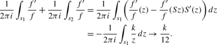
Comparing these two expressions for the integral, letting the radii of the small circular segments shrink to zero, one obtains the result.

If f has more poles or zeros on the boundary, the path of integration may be modified so as to circumvent these, as shown in the figure. □

Let $\mathcal{M}_{k}=\mathcal{M}_{k}(\varGamma_{0})$ be the complex vector space of all modular forms of weight k and let S _k be the space of cusp forms of weight k. Then $S_{k}\subset\mathcal{M}_{k}$ is the kernel of the linear map f↦f(i∞). By definition, it follows that

$$\mathcal{M}_k\mathcal{M}_l \subset \mathcal{M}_{k+l}, $$

which means that if $f\in\mathcal{M}_{k}$ and $g\in\mathcal{M}_{l}$, then $fg\in\mathcal{M}_{k+l}$.

Note that a holomorphic function f on ℍ with f| _k γ=f for every γ∈Γ ₀ lies in $\mathcal{M}_{k}$ if and only if the limit

$$\lim_{\operatorname{Im}(z)\to\infty}f(z) $$

exists.

The differential equation of the Weierstrass function ℘ features the coefficients

$$g_4 = 60 G_4,\qquad g_6=140 G_6. $$

It follows that g ₄(i∞)=120ζ(4) and g ₆(i∞)=280ζ(6). By Proposition 1.5.2 we have

$$\zeta(4)=\frac{\pi^4}{90},\quad\mbox{and}\quad\zeta(6) = \frac {\pi^6}{945}. $$

So with

$$\varDelta = g_4^3-27g_6^2, $$

it follows that Δ(i∞)=0, i.e. Δ is a cusp form of weight 12.

Theorem 2.2.12

Let k be an even integer.

• (a) If k<0 or k=2, then $\mathcal{M}_{k}=0$.

• (b) If k=0,4,6,8,10, then $\mathcal{M}_{k}$ is a one-dimensional vector space spanned by 1, G ₄, G ₆, G ₈, G ₁₀, respectively. In these cases the space S _k is zero.

• (c) Multiplication by Δ defines an isomorphism

  $$\mathcal{M}_{k-12}\stackrel{\cong}{\rightarrow} S_{k}. $$

Proof

Take a non-zero element $f\in\mathcal{M}_{k}$. All terms on the left of the equation

are ≥0. Therefore k≥0 and also k≠2, as 1/6 cannot be written in the form a+b/2+c/3 with a,b,c∈ℕ₀. This proves (a).

If 0≤k<12, then $\operatorname{ord}_{\infty}(f)=0$, and therefore S _k =0 and $\dim\mathcal{M}_{k}\le1$. This implies (b).

The function Δ has weight 12, so k=12. It is a cusp form, so $\operatorname{ord}_{\infty}(\varDelta )>0$. The formula implies $\operatorname{ord}_{\infty}(\varDelta )=1$ and that Δ has no further zeros. The multiplication with Δ gives an injective map $\mathcal{M}_{k-12}\to S_{k}$ and for 0≠f∈S _k we have $f/\varDelta \in\mathcal{M}_{k-12}$, so the multiplication with Δ is surjective, too. □

Corollary 2.2.13

• (a) One has

  

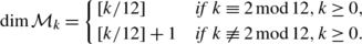
• (b) The space $\mathcal{M}_{k}$ has a basis consisting of all monomials $G_{4}^{m}G_{6}^{n}$ with m,n∈ℕ₀ and 4m+6n=k.

Proof

(a) follows from Theorem 2.2.12. For (b) we show that these monomials span the space $\mathcal{M}_{k}$. For k≤6, this is contained in Theorem 2.2.12. For k≥8 we use induction. Choose m,n∈ℕ₀ such that 4m+6n=k. The modular form $g=G_{4}^{m}G_{6}^{n}$ satisfies g(∞)≠0. Therefore, for given $f\in\mathcal{M}_{k}$ there is λ∈ℂ such that f−λg is a cusp form, i.e. equal to Δh for some $h\in\mathcal{M}_{k-12}$. By the induction hypothesis the function h lies in the span of the monomials indicated, and so does f.

It remains to show the linear independence of the monomials. Assume the contrary. Then a linear equation among these monomials of a fixed weight would lead to a polynomial equation satisfied by the function $G_{4}^{3}/G_{6}^{2}$, which would mean that this function is constant. This, however, is impossible, as the formula of Theorem 2.2.11 shows that G ₄ vanishes at ρ, but G ₆ does not. □

Let $M=\bigoplus_{k=0}^{\infty}\mathcal{M}_{k}$ be the graded algebra of all modular forms. One can formulate the corollary by saying that the map

$$\mathbb{C}[X,Y]\to M,\quad X\mapsto G_4,\ Y\mapsto G_6 $$

is an isomorphism of ℂ-algebras.

We have seen that

$$G_{k}(z) = 2\zeta(k)+2\frac{(2\pi i)^{k}}{(k-1)!}\sum _{n=1}^\infty \sigma_{k-1}(n)q^n, $$

where σ _k (n)=∑ _d|n d ^k. Denote the normalized Eisenstein series by E _k (z)=G _k (z)/(2ζ(k)). With $\gamma_{k}=(-1)^{k/2}\frac {2k}{B_{k/2}}$ we then have

$$E_{k}(z)= 1+\gamma_k\sum_{n=1}^\infty \sigma_{k-1}(n)q^n. $$

Examples

$$\everymath{\displaystyle} \begin{array}{rcl@{\qquad }lrcl} E_4 &=& 1+240\sum_{n=1}^\infty\sigma_3(n) q^n, & E_6 &=&1-504\sum_{n=1}^\infty\sigma_5(n) q^n,\\ E_8 &=&1+480\sum_{n=1}^\infty\sigma_7(n) q^n, & E_{10} &=&1-264\sum_{n=1}^\infty\sigma_9(n) q^n,\\ E_{12} &=&1+\frac{65520}{691}\sum_{n=1}^\infty\sigma_{11}(n) q^n.& \end{array} $$

Remark

As the spaces of modular forms of weights 8 and 10 are one-dimensional, we immediately get

$$E_4^2=E_8,\qquad E_4E_6=E_{10}. $$

These formulae are equivalent to

$$\sigma_7(n) = \sigma_3(n)+120\sum _{m=1}^{n-1}\sigma_3(m) \sigma_3(n-m) $$

and

$$11\sigma_9(n) = 21\sigma_5(n)-10 \sigma_3(n)+5040\sum_{m=1}^{n-1} \sigma_3(m)\sigma_5(n-m). $$

It is quite a non-trivial task to find proofs of these number-theoretical statements without using analysis!

2.3 Estimating Fourier Coefficients

Our goal is to attach so-called L-functions to modular forms by feeding their Fourier coefficients into Dirichlet series. In order to show convergence of these Dirichlet series, we must give growth estimates for the Fourier coefficients. Let

$$f(z) = \sum_{n=0}^\infty a_nq^n,\quad q= e^{2\pi iz} $$

be a modular form of weight k≥4.

Proposition 2.3.1

If f=G _k , then the Fourier coefficients a _n grow like n ^k−1. More precisely: there are constants A,B>0 with

$$An^{k-1} \le |a_n| \le Bn^{k-1}. $$

Proof

There is a positive number A>0 such that for n≥1 we have |a _n |=Aσ _k−1(n)≥An ^k−1. On the other hand,

$$\frac{|a_n|}{n^{k-1}} = A\sum_{d|n} \frac{1}{d^{k-1}} \le A\sum_{d=1}^\infty \frac{1}{d^{k-1}} = A\zeta(k-1) < \infty. $$

 □

Theorem 2.3.2

(Hecke)

The Fourier coefficients a _n of a cusp form f of weight k≥4 satisfy

$$a_n = O\bigl(n^{k/2}\bigr). $$

The O-notation means that there is a constant C>0 such that

$$|a_n|\le Cn^{k/2}. $$

Proof

Since f is a cusp form, it satisfies the estimate f(z)=O(q)=O(e ^−2πy) for q→0 or y→∞. Let ϕ(z)=y ^k/2|f(z)|. The function ϕ is invariant under the group Γ ₀. Furthermore, it is continuous and ϕ(z) tends to 0 for y→∞. So ϕ is bounded on the fundamental domain D of Sect. 2.1, so it is bounded on all of ℍ. This means that there exists a constant C>0 with |f(z)|≤Cy ^−k/2 for every z∈ℍ. By definition, $a_{n} = \int_{0}^{1} f(x+iy)q^{-n}\,dx$, so that |a _n |≤Cy ^−k/2 e ^2πny, and this estimate holds for every y>0. For y=1/n one gets |a _n |≤e ^2π Cn ^k/2. □

Remark

It is possible to improve the exponent. Deligne has shown that the Fourier coefficients of a cusp form satisfy

$$a_n = O\bigl(n^{\frac{k}{2}-\frac{1}{2}+\varepsilon }\bigr) $$

for every ε>0.

Corollary 2.3.3

For every $f\in\mathcal{M}_{k}(\varGamma_{0})$ with Fourier expansion

$$f(z)=\sum_{n=0}^\infty a_n e^{2\pi inz} $$

we have the estimate

$$a_n = O\bigl(n^{k-1}\bigr). $$

Proof

This follows from $\mathcal{M}_{k}= S_{k}+\mathbb{C}G_{k}$, as well as Proposition 2.3.1 and Theorem 2.3.2. □

2.4 L-Functions

In this section we encounter the question of why modular forms are so important for number theory. To each modular form f we attach an L-function L(f,s). These L-functions are conjectured to be universal in the sense that L-functions defined in entirely different settings are equal to modular L-functions. In the example of L-functions of (certain) elliptic curves this has been shown by Andrew Wiles, who used it to prove Fermat’s Last Theorem [Wil95].

Definition 2.4.1

For a cusp form f of weight k with Fourier expansion

$$f(z) = \sum_{n=1}^\infty a_n e^{2\pi inz}, $$

we define its L-series or L-function by

$$L(f,s) = \sum_{n=1}^\infty \frac{a_n}{n^s},\quad s\in\mathbb{C}. $$

Lemma 2.4.2

The series L(f,s) converges locally uniformly in the region $\operatorname{Re}(s)>\frac{k}{2}+1$.

Proof

From a _n =O(n ^k/2), as in Theorem 2.3.2, it follows that

$$a_n n^{-s}=O\bigl(n^{\frac{k}{2}-\operatorname{Re}(s)}\bigr), $$

which implies the claim. □

For the functional equation of the L-function we need the Gamma function, the definition of which we now recall.

Definition 2.4.3

The Gamma function is defined for $\operatorname{Re} (z)>0$ by the integral

$$\varGamma (z) = \int_0^\infty e^{-t}t^{z-1}\,dt. $$

Lemma 2.4.4

The Gamma integral converges locally uniformly absolutely in the right half plane $\operatorname{Re}(z)>0$ and defines a holomorphic function there. It satisfies the functional equation

$$\varGamma (z+1)=z\varGamma (z). $$

The Gamma function can be extended to a meromorphic function on ℂ, with simple poles at z=−n, n∈ℕ₀ and holomorphic otherwise. The residue at z=−n is $\frac{(-1)^{n}}{n!}$.

Proof

The function e ^−t decreases faster at +∞ than any power of t. Therefore the integral $\int_{1}^{\infty}e^{-t} t^{z-1}\,dt$ converges absolutely for every z∈ℂ and the convergence is locally uniform in z. For 0<t<1 the integrand is $\le t^{\operatorname{Re}(z)-1}$, so the integral $\int_{0}^{1} e^{-t}t^{z-1}\,dt$ converges locally uniformly for $\operatorname{Re}(z)>0$. As zt ^z−1 is the derivative of t ^z, we can use integration by parts to compute

$$z\varGamma (z) = \int_0^\infty e^{-t} \bigl(t^z\bigr)'\,dt = \underbrace {-e^{-t}t^z \big|_0^\infty}_{=0}+\underbrace{\int _0^\infty e^{-t}t^z \,dt}_{=\varGamma (z+1)}. $$

The function Γ(z) is holomorphic in $\operatorname{Re}(z)>0$. Using the formula

$$\varGamma (z)=\frac{1}{z}\varGamma (z+1), $$

we can extend the Gamma function to the region $\operatorname {Re}(z)>-1$ with a simple pole at z=0 of residue equal to $\varGamma (1)=\int_{0}^{\infty}e^{-t}\,dt=1$. This argument can be iterated to get the meromorphic continuation to all of ℂ. □

Theorem 2.4.5

Let f be a cusp form of weight k. Then the L-function L(f,s), initially holomorphic for $\operatorname {Re}(s)>\frac{k}{2}+1$, has an analytic continuation to an entire function. The extended function

$$\varLambda (f,s)\stackrel{\mathrm{def}}{=}(2\pi)^{-s}\varGamma (s) L(f,s) $$

is entire as well and satisfies the functional equation

$$\varLambda (f,s) = (-1)^{k/2}\varLambda (f,k-s). $$

The function Λ(f,s) is bounded on every vertical strip, i.e. for every T>0 there exists C _T >0 such that |Λ(f,s)|≤C _T for every s∈ℂ with $|\operatorname{Re}(s)|\le T$.

Proof

Let $f(z)=\sum_{n=1}^{\infty}a_{n}q^{n}$ with q=e ^2πiz be the Fourier expansion. According to Theorem 2.3.2 there is a constant C>0 such that |a _n |≤Cn ^k/2 holds for every n∈ℕ. So for given ε>0 we have for all y≥ε,

$$\big|f(iy)\big| = \Biggl \vert \sum_{n=1}^\infty a_n e^{-2\pi ny}\Biggr \vert \le C\sum _{n=1}^\infty n^{k/2} e^{-2\pi ny} \le De^{-\pi y}, $$

with $D=C\sum_{n=1}^{\infty}n^{k/2}e^{-\varepsilon \pi n}<\infty$. So the function f(iy) is rapidly decreasing as y→∞. The same estimate holds for the function $y\mapsto\sum_{n=1}^{\infty}|a_{n}|e^{-2\pi yn}$. Consequently, for every s∈ℂ we have

$$\int_\varepsilon^\infty\sum_{n=1}^\infty|a_n|e^{-2\pi yn}\big|y^{s-1}\big| \,dy < \infty. $$

Hence we are allowed to interchange sums and integrals in the following computation due to absolute convergence:

For $\operatorname{Re}(s)>\frac{k}{2}+1$ the right-hand side converges to

$$(2\pi)^{-s}\varGamma (s)L(f,s) = \varLambda (f,s), $$

as ε tends to zero. On the other hand, $f(i\frac{1}{y})=f(-\frac{1}{iy}) =(yi)^{k}f(iy)$, so that f(i/y) is also rapidly decreasing, and the left-hand side converges to $\int_{0}^{\infty}f(iy)y^{s-1}\,dy$, as ε→0. Together, for $\operatorname{Re}(s)>\frac{k}{2}+1$ we get

$$\int_0^\infty f(iy)y^{s-1}\,dy = \varLambda (f,s). $$

We write this integral as the sum $\int_{0}^{1}+\int_{1}^{\infty}$. As f(iy) is rapidly decreasing, the integral $\varLambda_{1}(f,s)=\int_{1}^{\infty}f(iy)y^{s-1}\,dy$ converges for every s∈ℂ and defines an entire function.

Because of

$$\big|\varLambda_1(f,s)\big| \le \int_1^\infty \big|f(iy)\big|y^{\operatorname{Re}(s)-1} \,dy, $$

the function Λ ₁(f,s) is bounded on every vertical strip.

For the second integral we have

$$\varLambda_2(f,s)=\int_0^1 f(iy)y^{s}\frac{dy}{y} = \int_1^\infty f\biggl(i\frac{1}{y}\biggr)y^{-s}\frac{dy}{y}= (-1)^{k/2} \int_1^\infty f(iy)y^{k-s} \frac{dy}{y}, $$

which means Λ ₂(f,s)=(−1)^k/2 Λ ₁(f,k−s), so the claim follows. □

Generally, a series of the form

$$L(s) = \sum_{n=1}^\infty\frac{a_n}{n^s} $$

for s∈ℂ, convergent or not, is called a Dirichlet series. The following typical convergence behavior of a Dirichlet series will be needed in the sequel.

Lemma 2.4.6

Let (a _n ) be a sequence of complex numbers. If for a given s ₀∈ℂ the sequence $\frac{a_{n}}{n^{s_{0}}}$ is bounded, then the Dirichlet series $L(s)=\sum_{n=1}^{\infty}\frac {a_{n}}{n^{s}}$ converges absolutely uniformly on every set of the form

$$\bigl\{ s\in\mathbb{C}: \operatorname{Re}(s)\ge\operatorname {Re}(s_0)+1+\varepsilon \bigr\}, $$

where ε>0.

This lemma reminds us of the convergence behavior of a power series. This is by no means an accident, as the power series with coefficients (a _n ) and the corresponding Dirichlet series are linked via the Mellin transform, as we shall see below.

Proof

Suppose that $|a_{n}n^{-s_{0}}|\le M$ for some M>0 and every n∈ℕ. Let ε>0 be given and let s∈ℂ with $\operatorname{Re}(s)\ge\operatorname{Re}(s_{0})+1+\varepsilon$. Then s=s ₀+α with $\operatorname{Re}(\alpha )\ge 1+\varepsilon$, and so

$$\biggl \vert \frac{a_n}{n^s}\biggr \vert = \biggl \vert \frac{a_n}{n^{s_0}} \biggr \vert \frac{1}{n^{\operatorname{Re}(\alpha )}} \le M\frac{1}{n^{1+\varepsilon }}. $$

As the series over 1/n ^1+ε converges, the lemma follows. □

Theorem 2.4.7

(Hecke’s converse theorem)

Let a _n be a sequence in ℂ, such that the Dirichlet series $L(s)=\sum_{n=1}^{\infty}a_{n} n^{-s}$ converges in the region $\{ \operatorname{Re} (s)>\nobreak C\}$ for some C∈ℝ. If the function Λ(s)=(2π)^−s Γ(s)L(s) extends to an entire function, which satisfies the functional equation

$$\varLambda (s)=(-1)^{k/2}\varLambda (k-s), $$

then there exists a cusp form f∈S _k with L(s)=L(f,s).

Proof

We use the inversion formula of the Fourier transform: For f∈L ¹(ℝ) let

$$\hat{f}(y) = \int_\mathbb{R}f(x)e^{-2\pi ixy}\,dx. $$

Suppose that f is two times continuously differentiable and that the functions f,f′,f″ are all in L ¹(ℝ). Then $\hat{f}(y)=O((1+|y|)^{-2})$, so that $\hat{f}\in L^{1}(\mathbb{R})$. Under these conditions, we have the Fourier inversion formula:

$$\skew{8}\hat{\hat{f}}(x) = f(-x). $$

A proof of this fact can be found in any of the books [Dei05, Rud87, SW71]. We use this formula here for the proof of the Mellin inversion formula.

Theorem 2.4.8

(Mellin inversion formula)

Suppose that the function g is two times continuously differentiable on the interval (0,∞) and for some c∈ℝ the functions

$$x^cg(x),\quad x^{c+1}g'(x),\quad x^{c+2}g''(x) $$

are all in $\in L^{1}(\mathbb{R}_{+},\frac{dx}{x})$. Then the Mellin transform

$$\mathcal{M}g(s)\stackrel{\mathrm{def}}{=}\int_0^\infty x^s g(x)\frac{dx}{x} $$

exists for $\operatorname{Re}(s)=c$, and satisfies the growth estimate $\mathcal{M} g(c+it)=O((1+|t|)^{-2})$. Finally, for every x∈(0,∞) one has the inversion formula:

$$g(x) = \frac{1}{2\pi i} \int_{c-i\infty}^{c+i\infty} x^{-s}\, \mathcal{M} g(s)\, ds. $$

Proof

A given s∈ℂ with $\operatorname{Re}(s)=c$ can be written as s=c−2πiy for a unique y∈ℝ. The substitution x=e ^t gives

$$\mathcal{M}g(s) = \int_\mathbb{R}e^{st}g \bigl(e^t\bigr)\,dt = \int_\mathbb {R}e^{ct}g\bigl(e^t\bigr) e^{-2\pi iyt}\,dt = \hat{F}(y), $$

with F(t)=e ^ct g(e ^t). The conditions imply that F is two times continuously differentiable and that F,F′,F″ are all in L ¹(ℝ). Further, one has $\hat{F}(y)=\mathcal{M}g(c-2\pi iy)$. By the Fourier inversion formula we deduce

The theorem is proven. □

We now show Hecke’s converse theorem. Let a _n be a sequence in ℂ, such that the Dirichlet series $L(s)=\sum_{n=1}^{\infty}a_{n} n^{-s}$ converges in the region $\{ \operatorname{Re} (s)> C\}$ for a given C∈ℝ. We define

$$f(z) = \sum_{n=1}^\infty a_n e^{2\pi inz}. $$

According to Lemma 2.4.6 there is a natural number N∈ℕ such that the Dirichlet series L(s) converges absolutely for $\operatorname{Re}(s)\ge N$. Therefore one has a _n =O(n ^N), so the series f(z) converges locally uniformly on the upper half plane ℍ and defines a holomorphic function there. We intend to show that it is a cusp form of weight k. Since the group Γ is generated by the elements S and T, it suffices to show that f(−1/z)=z ^k f(z). As f is holomorphic, it suffices to show that f(i/y)=(iy)^k f(iy) for y>0.

We first show that the Mellin transform of the function g(y)=f(iy) exists and that the Mellin inversion formula holds for g. We have

$$\big|f(iy)\big| = \Biggl \vert \sum_{n=1}^\infty a_n e^{-2\pi ny}\Biggr \vert \le \mbox{const}. \sum _{n=1}^\infty n^N e^{-2\pi ny}. $$

Denote $g_{N}(y)=\sum_{n=1}^{\infty}n^{N} e^{-2\pi ny}$. Let

$$g_0(y)=\sum_{n=0}^\infty e^{- 2\pi ny} = \frac{1}{1-e^{-2\pi y}} = \frac{1}{2\pi y}+h(y) $$

for some function h which is holomorphic in y=0. Then

$$g_N(y) = \frac{1}{(-2\pi)^N}g_0^{(N)}(y)= \frac{c_1}{y^{N+1}}+h^{(N)}(y), $$

so $|g_{N}(y)|\le\frac{C}{y^{N+1}}$ for y→0. The same estimate holds for f(iy). For y>1 the function |f(iy)| is less then a constant times

$$g_N(y)=\sum_{n=1}^\infty n^N e^{-2\pi ny} \le e^{-2\pi(y-1)}\sum _{n=1}^\infty n^N e^{-2\pi n} = e^{-2\pi y} e^{2\pi}g_N(1). $$

So the function f(iy) is rapidly decreasing for y→∞. The same estimates hold for every derivative of f, increasing N if necessary. So the Mellin integral $\mathcal{M}g(s)$ converges for $\operatorname{Re}(s)> N+1$ and since f(iy) is rapidly decreasing for y→∞, the conditions for the Mellin inversion formula are satisfied. Hence by Theorem 2.4.8 we have for every c>N+1,

$$f(iy)=\frac{1}{2\pi i}\int_{c-i\infty}^{c+i\infty} \varLambda (s) y^{-s}\,ds. $$

We next use a classical result of complex analysis, which itself follows from the maximum principle.

Lemma 2.4.9

(Phragmén–Lindelöf principle)

Let ϕ(s) be holomorphic in the strip $a\le\operatorname{Re}(s)\le b$ for some real numbers a<b. Assume there is α>0, such that for every a≤σ≤b we have $\phi(\sigma+it)=O(e^{|t|^{\alpha}})$. Suppose there is M∈ℝ with ϕ(σ+it)=O((1+|t|)^M) for σ=a and σ=b. Then we have ϕ(σ+it)=O((1+|t|)^M) uniformly for all σ∈[a,b].

Proof

See for instance [Con78], Chap. VI, or [Haz01, SS03]. □

We apply this principle to the case ϕ=Λ and a=k−c as well as b=c. We move the path of integration to $\operatorname{Re}(s)=c'=k-c$, where the integral also converges, according to the functional equation. This move of the integration path is possible by the Phragmén–Lindelöf principle. We infer that

2.5 Hecke Operators

We introduce Hecke operators, which are given by summation over cosets of matrices of fixed determinant. In later chapters, we shall encounter a reinterpretation of these operators in the adelic setting.

For given n∈ℕ let M _n denote the set of all matrices in M₂(ℤ) of determinant n. The group Γ ₀=SL₂(ℤ) acts on M _n by multiplication from the left.

Lemma 2.5.1

The set M _n decomposes into finitely many Γ ₀-orbits under multiplication from the left. More precisely, the set

$$R_n=\left \{ \left(\matrix{ a& b\cr& d}\right) : a,d\in\mathbb{N},\ ad=n,\ 0\le b <d \right \} $$

is a set of representatives of Γ ₀∖M _n .

Notation

Here and for the rest of the book we use the convention that a zero entry of a matrix may be left out, so stands for the matrix .

Proof

We have to show that every Γ ₀-orbit meets the set R _n in exactly one element. For this let . For x∈ℤ we have

$$\left(\matrix{1& \cr x&1}\right) \left(\matrix{a& b\cr c&d}\right) = \left(\matrix{a&b\cr c+ax& d+bx}\right). $$

This implies that, modulo Γ ₀, we can assume 0≤c<|a|. By the identity

$$\left(\matrix{&{-1}\cr1&}\right) \left(\matrix{a& b\cr c& d}\right) = \left(\matrix{-c&-d\cr a&b}\right) $$

one can interchange a and c, then reduce again by the first step and iterate this process until one gets c=0, which implies that every Γ ₀-orbit contains an element of the form . Then ad=det=n, and since −1∈Γ ₀ one can assume a,d∈ℕ. By

$$\left(\matrix{1& x\cr&1}\right) \left(\matrix{a&b\cr& d}\right)= \left(\matrix{a& {b+dx}\cr& d}\right) $$

one can finally reduce to 0≤b<d, so every Γ ₀-orbit meets the set R _n .

In order to show that R _n is a proper set of representatives, it remains to show that two elements in R _n , which lie in the same Γ ₀-orbit, are equal. For this let be in the same Γ ₀-orbit. This means that there is with

$$\left(\matrix{a'& b'\cr& d'}\right) = \left(\matrix{x&y\cr z& w}\right) \left(\matrix{a& b\cr&d}\right). $$

The right-hand side is of the form . Since a≠0, we infer that z=0. Then xw=1, so x=w=±1. Because of

$$\left(\matrix{x& y\cr& w}\right) \left(\matrix{a& b\cr&d}\right)= \left(\matrix{ax& *\cr& *}\right) $$

one has a′=ax>0, so x>0 and therefore x=1=w, so a′=a and d′=d. It follows that

$$\left(\matrix{a& {b'}\cr& d}\right)= \left(\matrix{ 1& y\cr& 1}\right) \left(\matrix{a& b\cr&d}\right) = \left(\matrix{a& {b+dy}\cr& d}\right), $$

so that the condition 0≤b,b′<d finally forces b=b′. □

Let $\operatorname{GL}_{2}(\mathbb{R})^{+}$ be the set of all $g\in \operatorname{GL}_{2}(\mathbb{R})$ of positive determinants. The group $\operatorname{GL}_{2}(\mathbb{R})^{+}$ acts on the upper half plane ℍ by

$$\left(\matrix{ a&b\cr c&d }\right)z = \frac{az+b}{cz+d}. $$

The center acts trivially.

For k∈2ℤ, a function f on ℍ and we write

$$f|_{k}\gamma(z) = \det(\gamma)^{k/2}(cz+d)^{-k}f \biggl(\frac{az+b}{cz+d}\biggr). $$

If k is fixed, we also use the simpler notation f|γ(z). Note that the power k/2 of the determinant factor has been chosen so that the center of $\operatorname{GL}_{n}(\mathbb{R})^{+}$ acts trivially.

We write Γ ₀=SL₂(ℤ). For n∈ℕ define the Hecke operator T _n as follows.

Definition 2.5.2

Denote by V the vector space of all functions f:ℍ→ℂ with f|γ=f for every γ∈Γ ₀. Define T _n :V→V by

$$T_nf = n^{\frac{k}{2}-1}\sum_{y:\varGamma _0\backslash M_n}f|y, $$

where the colon means that the sum runs over an arbitrary set of representatives of Γ ₀∖M _n in M _n . The factor $n^{\frac{k}{2}-1}$ is for normalization only. The sum is well defined and finite, as f|γ=f for every γ∈Γ ₀ and Γ ₀∖M _n is finite. In order to show that T _n f indeed lies in the space V, we compute for γ∈Γ ₀,

$$T_nf|\gamma= n^{\frac{k}{2}-1}\sum_{y:\varGamma _0\backslash M_n}(f|y)| \gamma= n^{\frac{k}{2}-1}\sum_{y:\varGamma _0\backslash M_n}f|y\gamma = n^{\frac{k}{2}-1}\sum_{y:\varGamma _0\backslash M_n}f|y = T_nf. $$

Using Lemma 2.5.1 we can write

Lemma 2.5.3

The Hecke operator T _n preserves the spaces $\mathcal{M}_{k}(\varGamma_{0})$ and S _k (Γ ₀).

Proof

We have just shown that for a given $f\in\mathcal{M}_{k}(\varGamma_{0})$ the function T _n f is invariant under the action of Γ ₀. Being a finite sum of holomorphic functions, the function T _n f is holomorphic on ℍ. To show that T _n f is a modular form, we write

This formula shows that T _n f(z) converges as $\operatorname {Im}(z)\to\infty$, since f(z) does. This means that $T_{n}f\in\mathcal{M}_{k}(\varGamma_{0})$. If f is a cusp form, the limit is zero and the same holds for T _n f. □

Proposition 2.5.4

The Hecke operators satisfy the equations

• $T_{1}=\operatorname{Id}$,

• T _mn =T _m T _n , if $\operatorname{gcd}(m,n)=1$,

• for every prime number p and every n∈ℕ one has $T_{p}T_{p^{n}} = T_{p^{n+1}}+p^{k-1}T_{p^{n-1}}$.

Together these equations imply that T _n T _m =T _m T _n always, i.e. all Hecke operators commute with each other.

Proof

The first assertion is trivial. For the second note

$$|R_n| = \sum_{d|n}d = \sigma_1(n). $$

If m,n∈ℕ are coprime, then it follows that |R _mn |=|R _m ||R _n |. To ease the presentation we will, in the following calculations, in an integer matrix , consider the number b only modulo d. Under this proviso, we show that the map

$$R_n\times R_m\to R_{mn},\quad(A,B)\mapsto AB $$

is a bijection, where we still assume that m and n are coprime. As both sets have the same cardinality, it suffices to show injectivity. So let

Then aa′=αα′ and since (m,n)=1, it follows that a=α and a′=α′. Analogously for d and δ. So we have

$$ab'+bd'\equiv a\beta'+\beta d'\operatorname{mod}\bigl(dd'\bigr). $$

Reduction modulo d′ gives

$$ab'\equiv a\beta'\operatorname{mod} \bigl(d'\bigr). $$

Being a divisor of n, the number a is coprime to d′, so $b'\equiv \beta'\operatorname{mod}(d')$. In the same way we get $b\equiv\beta\operatorname{mod}d$. Hence R _m R _n =R _mn and so

For the last point note

$$R_p = \left \{\left(\matrix{ p&\cr& 1}\right) \right \}\cup \left \{ \left(\matrix{1& b\cr& p}\right): b\operatorname{mod}p \right \}, $$

as well as

It follows that

The second set, together with , is a set of representatives $R_{p^{n+1}}$. The sum over this gives the term $T_{p^{n+1}}$. The first set minus is

Denote this last set by S. Since the central p acts trivially, one gets

$$\bigl(p^{n+1}\bigr)^{\frac{k}{2}-1}\sum_{y\in S}f|y = \bigl(p^{n+1}\bigr)^{\frac{k}{2}-1}p\sum_{y\in R_{p^{n-1}}} f|y = p^{k-1}T_{p^{n-1}}f. $$

 □

We now want to see how the application of a Hecke operator changes the Fourier expansion of a modular form.

Proposition 2.5.5

For a given form $f(z)=\sum_{m\ge0}c(m)q^{m}\in\mathcal{M}_{k}$ and n∈ℕ the Fourier expansion of T _n f is

$$T_nf(z) = \sum_{m\ge0} \gamma(m)q^m $$

with

Proof

By definition we have

The sum ∑_0≤b<d e ^2πibm/d equals d if d|m and 0 otherwise. Setting m′=m/d one gets

Sorting this by powers of q results in

The proposition is proven. □

The following two corollaries are simple consequences of the proposition.

Corollary 2.5.6

One has γ(0)=σ _k−1(n)c(0) and γ(1)=c(n).

Corollary 2.5.7

If p is a prime number, then

$$\everymath{\displaystyle} \begin{array}{rcl@{\quad }l} \gamma(m) &=& c(pm) &\mathit{if}\ m\not\equiv0\operatorname {mod}(p),\\[6pt] \gamma(m) &=&c(pm)+p^{k-1}c(m/p),&\mathit{if}\ m\equiv0\operatorname{mod}(p). \end{array} $$

In Proposition 2.5.4 we have shown that Hecke operators commute with each other. We next show that they can be diagonalized simultaneously.

Lemma 2.5.8

A set of commuting self-adjoint operators on a finite-dimensional unitary space can be simultaneously diagonalized.

We elaborate the formulation of this lemma as follows: let V be a finite-dimensional complex vector space equipped with an inner product 〈.,.〉 and let $E\subset\operatorname{End}(V)$ be a set of self-adjoint operators on V. Suppose that any two elements S,T∈E commute, i.e. ST=TS. Then there exists a basis of V such that all elements of E are represented by diagonal matrices with respect to that basis. More precisely, this basis, say v ₁,…,v _n , consists of simultaneous eigenvectors, so for each 1≤j≤n there exists a map χ _j :E→ℂ such that

$$Tv_j=\chi_j(T)v_j $$

holds for every T∈E.

Proof

We prove the lemma by induction on the dimension of V. If dim(V)=1, then there is nothing to show. So suppose dim(V)>1 and that the claim is proven for all spaces of smaller dimension. If all T∈E are multiples of the identity, i.e. $T=\lambda \operatorname{Id}$ for some λ=λ(T)∈ℂ, then the claim follows. So assume there exists a T∈E not a multiple of the identity. Since T is self-adjoint, it is diagonalizable, so V is the direct sum of the eigenspaces of T, and each eigenspace is of dimension strictly smaller than dim(V). Let S∈E and let V _λ be the T-eigenspace for the eigenvalue λ. We claim that S(V _λ )⊂V _λ . For a given v∈V _λ we have

$$T\bigl(S(v)\bigr)=S\bigl(T(v)\bigr)=S(\lambda v)=\lambda S(v), $$

i.e. S(v)∈V _λ and the space V _λ is stable under all S∈E and by the induction hypothesis, V _λ has a basis of simultaneous eigenvectors. As this holds for all eigenvalues of T, the entire space V has such a basis. □

Definition 2.5.9

Let E be as in the lemma. Then V has a basis v ₁,…,v _n such that for every S∈E,

$$Sv_j = \chi_j(S)v_j $$

for a scalar χ _j (S)∈ℂ. We say, the v _j are simultaneous eigenvectors of E.

Recall the notion of a complex algebra. This is a ℂ-vector space A with a bilinear map A×A→A written (a,b)↦ab, which is associative, i.e. one has

$$(ab)c=a(bc) $$

for all a,b,c∈A.

Examples 2.5.10

• The set M _n (ℂ) of complex n×n matrices is a complex algebra which is isomorphic to the algebra $\operatorname{End}(V)$ of linear endomorphisms of a complex vector space of dimension n. Giving an isomorphism $\operatorname{End}(V)\cong\mathrm {M}_{n}(\mathbb{C})$ is equivalent to choosing a basis of V.

• The set $\mathcal{B}(V)$ of bounded linear operators on a Banach space V is a complex algebra.

• Let $\emptyset\ne E\subset\operatorname{End}(V)$ for a vector space V. The algebra generated by E is the set of all linear combinations of operators of the form S ₁⋯S _n , where S ₁,…,S _n ∈E. It is the smallest algebra which contains E.

Denote by $\mathcal{A}$ the algebra generated by E. Then the v _j are simultaneous eigenvectors for the whole of $\mathcal{A}$, and the maps χ _j can be extended to maps $\chi_{j}:\mathcal{A}\to\mathbb{C}$, such that for every operator $T\in\mathcal{A}$ the eigen-equation Tv _j =χ _j (T)v holds. Note that for $S,T\in\mathcal{A}$ one has

$$\chi_j(S+T)v_j = (S+T)v_j = Sv_j+Tv_j = \chi(S)v_j+ \chi(T)v_j, $$

so χ _j (S+T)=χ _j (S)+χ _j (T). Further χ _j (λT)=λχ _j (T) for every λ∈ℂ; this means that each χ _j is a linear map. More than that, one has

$$\chi_j(ST)v_j = STv_j = S \bigl(T(v_j)\bigr) = S\bigl(\chi_j(T)v_j \bigr) = \chi_j(T)S(v_j) = \chi_j(T) \chi_j(S)v_j, $$

so it even follows χ _j (ST)=χ _j (S)χ _j (T), i.e. the map χ _j is multiplicative. Together this means: every χ _j is an algebra homomorphism of the algebra $\mathcal{A}$ to ℂ.

In the sequel, we shall need to following theorem, known as the Elementary Divisor Theorem.

Theorem 2.5.11

(Elementary Divisor Theorem)

For a given integer matrix A∈M _n (ℤ) with det(A)≠0 there exist invertible matrices $S,T\in\operatorname{GL}_{n}(\mathbb{Z})$ and natural numbers d ₁,d ₂,…,d _n with d _j |d _j+1 such that

$$A=S\left ( \begin{array}{c@{\quad }c@{\quad }c}d_1 & & \\ & \ddots& \\ & & d_n \end{array} \right )T. $$

The numbers d ₁,…,d _n are uniquely determined by A and are called the elementary divisors of A.

Proof

For example in [HH80]. □

Definition 2.5.12

Denote by $\operatorname{GL}_{2}(\mathbb{Q})^{+}$ the set of all matrices $g\in\operatorname{GL}_{2}(\mathbb{Q})$ with det(g)>0. This is a subgroup of the group $\operatorname{GL}_{2}(\mathbb{Q})$ of index 2.

Proposition 2.5.13

We continue to write Γ ₀=SL₂(ℤ). A complete set of representatives of the double quotient

$$\varGamma_0\backslash \operatorname{GL}_2( \mathbb{Q})^+/\varGamma_0 $$

is given by the set of all diagonal matrices , where a∈ℚ and n∈ℕ.

Proof

For a given $\alpha \in\operatorname{GL}_{2}(\mathbb{Q})^{+}$ there exists N∈ℕ, such that Nα is an integer matrix. By the Elementary Divisor Theorem there are $S,T\in\operatorname{GL}_{2}(\mathbb{Z})$ such that Nα=SDT, where with d ₁,n∈ℕ. If necessary, one can multiply S and T with the matrix , so that S,T∈SL₂(ℤ) can be assumed. Therefore we find . The uniqueness of the representative follows from the Elementary Divisor Theorem, if one chooses N as the unique smallest N∈ℕ making Nα an integer matrix. □

Corollary 2.5.14

For given $g\in\operatorname{GL}_{2}(\mathbb{Q})^{+}$ and Γ ₀=SL₂(ℤ) one has

$$\varGamma_0 g^{-1}\varGamma_0 = \frac{1}{ \det(g)}\varGamma_0 g\varGamma_0. $$

Proof

By the proposition we can assume that g is a diagonal matrix . Then and this last matrix lies in the same double Γ ₀-coset as g, since

$$\left(\matrix{&{-1}\cr1&}\right) \left(\matrix{{an}&\cr& a}\right) \left(\matrix{& 1\cr{-1}&}\right)= \left(\matrix{a& \cr& {an}}\right), $$

so the corollary is proven. □

We have seen that the group G=SL₂(ℝ) acts on the upper half plane ℍ via

$$\left(\matrix{a&b\cr c&d}\right)z = \frac{az+b}{cz+d}. $$

Lemma 2.5.15

The measure $d\mu=\frac{dx\,dy}{y^{2}}$ on ℍ is invariant under the action of G, i.e. we have

$$\int_\mathbb{H}f(z)\,d\mu(z)=\int_\mathbb{H}f(gz) \,d\mu(z) $$

for every integrable function f and every g∈G.

Proof

Every g∈G defines a holomorphic map z↦gz on ℍ. We compute its differential as

$$g'z=\frac{d(gz)}{dz}=\frac{a(cz+d)-c(az+b)}{(cz+d)^2}=\frac{1}{(cz+d)^2}. $$

This is equivalent to the identity of differential forms

$$d(gz)=\frac{1}{(cz+d)^2}dz, $$

where dz=dx+idy and d(gz) is the pullback of dz under g. Applying complex conjugation yields $\overline{dz}=dx-idy$, so $dz\wedge\overline{dz}=-2i (dx\wedge dy)$. Further, by the above,

$$d(gz)\wedge\overline{d(gz)}=\frac{1}{|cz+d|^4} dz\wedge\overline {dz}= \frac{\operatorname{Im}(gz)^2}{\operatorname{Im}(z)^2}dz\wedge \overline{dz}, $$

or

$$\frac{d(gz)\wedge\overline{d(gz)}}{\operatorname{Im}(gz)^2}=\frac {dz\wedge \overline{dz}}{\operatorname{Im}(z)^2}, $$

which is to say that the differential form $\frac{dz\wedge\overline {dz}}{\operatorname{Im}(z)^{2}}$ is invariant under G. This implies the claim. □

This lemma can also be proved without the use of differential forms; see Exercise 2.8.

Theorem 2.5.16

The spaces $\mathcal{M}_{k}$ and S _k have bases consisting of simultaneous eigenvectors of all Hecke operators.

Proof

We want to apply the lemma with E={T _n :n∈ℕ}. For this we have to define an inner product on $\mathcal{M}_{k}$. For given $f,g\in\mathcal{M}_{k}$ the function $f(z)\overline{g(z)}y^{k}$ is invariant under the group Γ ₀. It is a continuous, hence measurable, function on the quotient Γ ₀∖ℍ. The measure $\frac{dx\,dy}{y^{2}}$ is Γ ₀-invariant as well, and hence defines a measure μ on Γ ₀∖ℍ. This is an important point, so we will explain it a bit further. One way to view this measure on the quotient Γ ₀∖ℍ is to identify Γ ₀∖ℍ with a measurable set of representatives R with $D\subset R\subset \overline{D}$, where D is the standard fundamental domain of Definition 2.1.6. Then any measurable subset A⊂Γ ₀∖ℍ can be viewed as a subset of R⊂ℍ and the measure $\frac{dx\,dy}{y^{2}}$ can be applied. Interestingly, the measure μ on Γ ₀∖ℍ is a finite measure, i.e.

$$\mu(\varGamma_0\backslash \mathbb{H}) < \infty, $$

as the $\frac{dx\, dy}{y^{2}}$-measure of $\overline{D}$ is finite by Exercise 2.9. According to Exercise 2.15 the integral

$$\langle f,g\rangle_{\operatorname{Pet}}= \int_{\varGamma _0\backslash \mathbb{H}}f(z) \overline{g(z)}y^{k}\frac {dx\,dy}{y^2} $$

exists if one of the two functions f,g is a cusp form. This integral defines an inner product on the space S _k , which is called the Petersson inner product. We show that $\langle T_{n}f,g\rangle_{\operatorname{Pet}}=\langle f,T_{n}g\rangle_{\operatorname{Pet}}$, so the T _n are self-adjoint on the space S _k . This implies the claim on S _k . The space $S_{k}^{\perp}=\{ f\in\mathcal{M}_{k}:\langle f,g\rangle_{\operatorname{Pet}}=0\ \forall g\in S_{k}\}$ is one-dimensional if $\mathcal{M}_{k}\ne0$. By the self-adjointness of the Hecke operators, this space is T _n -invariant as well, so, being one-dimensional, it is a simultaneous eigenspace. It only remains to show the claimed self-adjointness.

We do this by extending the Petersson inner product to functions which are not necessarily invariant under Γ ₀, but only under a subgroup of finite index in Γ ₀. We first consider the case k=0. Take two continuous and bounded functions f,g on ℍ, which are invariant under Γ ₀, so they satisfy f(γz)=f(z) for every z∈ℍ and every γ∈Γ ₀, and the same for the function g. Then we define

$$\langle f,g\rangle = \int_{\varGamma _0\backslash \mathbb {H}}f(z)\overline{g(z)}\,d\mu(z), $$

where μ is the measure $\frac{dx\,dy}{y^{2}}$. The integral exists, since f and g are bounded and Γ ₀∖ℍ has finite measure, as we have seen above. We now make a crucial observation: If Γ⊂Γ ₀ is a subgroup of finite index, then

$$\langle f,g\rangle = \frac{1}{[\overline{\varGamma }_0:\overline { \varGamma }]}\int_{\varGamma \backslash \mathbb{H}} f(z)\overline{g(z)}\,d\mu(z), $$

where, as in Definition 2.1.6, the group $\overline{\varGamma }_{0}$ is Γ ₀/±1 and $\overline {\varGamma }$ is the image of Γ in $\overline{\varGamma }_{0}$. If the functions f and g are continuous and bounded, but only invariant under Γ and no longer invariant under Γ ₀, then the last expression still does make sense. This means that we can define 〈f,g〉 in this more general situation by the expression

$$\langle f,g\rangle\stackrel{\mathrm{def}}{=}\frac{1}{[\overline {\varGamma }_0:\overline{\varGamma }]}\int_{\varGamma \backslash \mathbb{H}} f(z) \overline{g(z)}\,d\mu(z). $$

In this way we extend the definition of the Petersson inner product in the case k=0. In the case k>0 we consider two continuous functions f,g with f| _k σ=f for every σ∈Γ, and the same for g. We assume that the Γ-invariant function |f(z)y ^k/2| is bounded on the upper half plane ℍ and the same for g. We then define

$$\langle f,g\rangle_{k}\stackrel{\mathrm{def}}{=}\frac{1}{[\overline { \varGamma }_0:\overline{\varGamma }]}\int_{\varGamma \backslash \mathbb{H}}f(z) \overline{g(z)}y^{k}\,d\mu(z). $$

We claim that for a given $\alpha \in\operatorname{GL}_{2}(\mathbb {Q})^{+}$ the group Γ=α ⁻¹ Γ ₀ α∩Γ ₀ is a subgroup of Γ ₀ of finite index.

Proof of This Claim

By Proposition 2.5.13 we can assume with r∈ℚ and n∈ℕ. Then

$$\alpha^{-1}\left(\matrix{a&b\cr c&d}\right)\alpha = \left(\matrix{a& {nb}\cr\frac{c}{n}&d}\right). $$

So a given lies in Γ if and only if c/n∈ℤ, i.e. if n divides c. Therefore the group Γ contains the group Γ(n) of all matrices γ∈SL₂(ℤ) with . This group is by definition the kernel of the group homomorphism SL₂(ℤ)→SL₂(ℤ/nℤ), which comes from the reduction homomorphism ℤ→ℤ/nℤ. As the group SL₂(ℤ/nℤ) is finite, the group Γ has finite index in Γ ₀.

Definition 2.5.17

Let Γ⊂SL₂(ℤ) be a subgroup. A fundamental domain for Γ is an open subset F⊂ℍ, such that there is a set R⊂ℍ of representatives for Γ∖ℍ with

$$F \subset R \subset \overline{F} \quad\mbox{and}\quad\mu(\overline{F} \smallsetminus {F}) = 0, $$

where μ is the measure $\frac{dx\,dy}{y^{2}}$.

In particular, if F is a fundamental domain for Γ, then $\bigcup_{\sigma\in\varGamma }\sigma\overline{F} = \mathbb{H}$, so every point in ℍ lies in a Γ-translate of $\overline{F}$.

Lemma 2.5.18

Let F⊂ℍ be a fundamental domain for the group Γ⊂SL₂(ℤ). For every measurable, Γ-invariant function f on ℍ one has

$$\int_Ff(z)\,d\mu(z) = \int_{\varGamma \backslash \mathbb{H}}f(z) \, d\mu(z), $$

where $\mu=\frac{dx\,dy}{y^{2}}$ is the invariant measure. So in particular, the first integral exists if and only if the second does.

Proof

The projection p:ℍ→Γ∖ℍ maps F injectively onto a subset, whose complement is of measure zero. Therefore ∫ _Γ∖ℍ f(z) dμ(z)=∫ _p(F) f(z) dμ(z). Since the measure on the quotient is defined by the measure on ℍ, the bijection p:F→p(F) preserves measures. This implies the claim. □

Lemma 2.5.19

• (a) D is a fundamental domain for Γ ₀=SL₂(ℤ).

• (b) If Γ is a subgroup of Γ ₀=SL₂(ℤ) of finite index and S is a set of representatives of $\overline{\varGamma }\backslash \overline{\varGamma }_{0}$, then

  $$SD = \bigcup_{\gamma\in S}\gamma D $$

  is a fundamental domain for the group Γ. The set $S\subset\overline{\varGamma }_{0}$ is uniquely determined by the fundamental domain SD.

Proof

Part (a) follows from Theorem 2.1.7.

(b) The set S is finite, as Γ has finite index in Γ ₀. Hence it follows that $\overline{SD}=\bigcup_{\gamma\in S}\gamma \overline{D}$. Now let $R_{\varGamma _{0}}$ be a set of representatives of Γ ₀∖ℍ with $D\subset R_{\varGamma _{0}}\subset\overline{D}$. Then $R_{\varGamma}=\bigcup_{\gamma\in S}\gamma R_{\varGamma _{0}}$ is a set of representatives of Γ∖ℍ with $SD\subset R_{\varGamma}\subset\overline{SD}$. Further one has

The last assertion follows from the fact that for γ≠τ in $\overline{\varGamma }_{0}$ the translates γD and τD are disjoint. □

The points $\gamma\infty\in\widehat{\mathbb{R}}$ for γ∈S are called the cusps of the fundamental domain SD. These lie in $\widehat{\mathbb{Q}}=\mathbb{Q}\cup\{\infty\}$. The wording becomes clearer, when one considers the unit disk instead of the upper half plane. So let $\mathbb{E}=\{ z\in\mathbb{C}: |z|<1\}$ be the open unit disk. The Cayley map:

$$\tau(z)\stackrel{\mathrm{def}}{=}\frac{z-i}{z+i} $$

is a bijection from ℍ to $\mathbb{E}$ such that τ as well as its inverse τ ⁻¹ are both holomorphic. Transporting the fundamental domain SD into E by means of the map τ, the cusps are the points where the fundamental domain touches the boundary of the disk, i.e. the unit circle. Each cusp is the endpoint of two circles which lie inside E and are orthogonal to the unit circle, so they are tangential at the cusp, i.e. the cusp is ‘infinitesimally sharp’, which explains the name ‘cusp’. The next figure shows a fundamental domain F with one cusp.

As the specific choice of a set of representatives S is not important, we frequently write D _Γ for the fundamental domain SD.

Lemma 2.5.20

The Petersson inner product is invariant under $\operatorname {GL}_{2}(\mathbb{Q})^{+}$, which means the following: For given $f,g\in\mathcal{M}_{k}$, one of them in S _k and for each $\alpha \in\operatorname{GL}_{2}(\mathbb{Q})^{+}$, the inner product 〈f|α,g|α〉 _k is defined in the above sense with Γ=αΓ ₀ α ⁻¹∩Γ ₀, and it holds that

$$\langle f|\alpha ,g|\alpha \rangle_{k}=\langle f,g \rangle_{k}. $$

Proof

Let Γ ₀=SL₂(ℤ) and Γ=αΓ ₀ α ⁻¹∩Γ ₀, as well as Γ′=α ⁻¹ Γα=α ⁻¹ Γ ₀ α∩Γ ₀. For given $f\in\mathcal{M}_{k}$ the function h=f|α has the property that h|σ=h for every σ∈Γ′, since σ=α ⁻¹ γα for some γ∈Γ ₀, so

$$h|\sigma=f|\alpha \sigma= f|\gamma\alpha = f|\alpha = h. $$

The same holds for g, so the inner product 〈f|α,g|α〉 is well defined. Note that for we have

$$\operatorname{Im}(\alpha z) = \det\alpha \frac{\operatorname {Im}(z)}{|cz+d|^2}. $$

In the following calculation we use the $\operatorname{GL}_{2}(\mathbb{Q})^{+}$-invariance of the measure μ together with the fact that we may replace integration over Γ∖ℍ with integration over a fundamental domain according to Lemma 2.5.18. We further use that α ⁻¹ D _Γ is a fundamental domain for Γ′ to get

Finally we have $[\overline{\varGamma }_{0}:\overline{\varGamma }]=[\overline{\varGamma }_{0}:\overline{\varGamma }']$, since $[\overline{\varGamma }_{0}:\overline{\varGamma }] = \mu(D_{\varGamma})/\mu (D) = \mu(\alpha^{-1}D_{\varGamma})/\mu(D) = [\overline{\varGamma }_{0}:\overline{\varGamma }']$. □

The lemma implies for $y\in\operatorname{GL}_{2}(\mathbb{Q})^{+}$,

$$\langle f|y,g\rangle = \bigl\langle f|y|y^{-1},g|y^{-1}\bigr \rangle = \bigl\langle f,g|y^{-1}\bigr\rangle, $$

hence,

$$\langle T_nf,g\rangle = n^{k-1}\sum _{y:\varGamma _0\backslash M_n}\langle f|y,g\rangle = n^{k-1}\sum _{y:\varGamma _0\backslash M_n}\bigl\langle f,g|y^{-1}\bigr\rangle. $$

As f and g are both invariant under Γ ₀, the expression 〈f,g|y ⁻¹〉 depends only on the double coset Γ ₀ y ⁻¹ Γ ₀. By Corollary 2.5.14, this double coset equals $\varGamma_{0}\frac{1}{\det (y)}y\varGamma_{0}$. The center acting trivially on $\mathcal{M}_{k}$, this matrix acts like y. Therefore,

$$\langle T_nf,g\rangle = n^{k-1}\sum _{y:\varGamma _0\backslash M_n}\langle f,g|y\rangle = \langle f,T_ng \rangle. $$

It follows that there are bases of $\mathcal{M}_{k}$ and S _k consisting of simultaneous eigenvectors of all Hecke operators. Theorem 2.5.16 follows.  □

Theorem 2.5.21

Let $f(z)=\sum_{n=0}^{\infty}c(n)q^{n}$ be a non-constant simultaneous eigenfunction of all Hecke operators, i.e. for every n∈ℕ there is a number λ(n)∈ℂ such that T _n f=λ(n)f.

• (a) The coefficient c(1) is not zero.

• (b) If c(1)=1, which can be reached by scaling f, then c(n)=λ(n) for every n∈ℕ.

Proof

By Corollary 2.5.6 the coefficient of q in T _n f equals c(n). On the other hand, this coefficient equals λ(n)c(1). Therefore, c(1)=0 would lead to c(n)=0 for all n, hence f=0. Both claims follow. □

A Hecke eigenform $f\in\mathcal{M}_{k}$ is called normalized if the coefficient c(1) is equal to 1.

Corollary 2.5.22

Let k>0. Two normalized Hecke eigenforms, which share the same Hecke eigenvalues, coincide.

Proof

Let $f,g\in\mathcal{M}_{k}$ with T _n f=λ(n)f and T _n g=λ(n)g for every n∈ℕ. By the theorem, all coefficients of the q-expansions of f and g coincide, with the possible exception of the zeroth coefficients. This means that f−g is constant. As k>0, there are no constant modular forms of weight k other than zero. We conclude f=g. □

Corollary 2.5.23

For a normalized Hecke eigenform $f(z) = \sum_{n=0}^{\infty}c(n)q^{n}$ we have

• c(mn)=c(m)c(n) if $\operatorname{gcd}(m,n)=1$,

• c(p)c(p ⁿ)=c(p ⁿ⁺¹)+p ^k−1 c(p ⁿ⁻¹), n≥1.

Proof

The assertion follows from the corresponding relations for Hecke operators in Proposition 2.5.4. □

Definition 2.5.24

We say that a Dirichlet series $L(s)=\sum_{n=1}^{\infty}a_{n}n^{-s}$, which converges in some half plane $\{\operatorname{Re}(s)>a\}$, has an Euler product of degree k∈ℕ, if for every prime p there is a polynomial

$$Q_p(x)=1+a_{p,1}x+\cdots+a_{p,k}x^{k} $$

such that in the domain $\operatorname{Re}(s)>a$ one has

$$L(s)=\prod_{p}\frac{1}{Q_p (p^{-s})}. $$

Example 2.5.25

The Riemann zeta function $\zeta(s)=\sum_{n=1}^{\infty}n^{-s}$, convergent for $\operatorname{Re}(s)>1$, has the Euler product

$$\zeta(s)=\prod_p\frac{1}{1-p^{-s}}; $$

see Exercise 1.5.

Corollary 2.5.26

The L-function $L(f,s)=\sum_{n=1}^{\infty}c(n) n^{-s}$ of a normalized Hecke eigenform $f(z)=\sum_{n=0}^{\infty}c(n)q^{n}\in\mathcal{M}_{k}$ has an Euler product:

$$L(f,s) = \prod_{p}\frac{1}{1-c(p)p^{-s}+p^{k-1-2s}}, $$

which converges locally uniformly absolutely for $\operatorname{Re}(s)>k$.

Proof

By Corollary 2.3.3 the coefficients grow at most like c(n)=O(n ^k−1). So the L-series converges locally uniformly absolutely for $\operatorname{Re}(s)>k$. The partial sum

$$\sum_{n\in p^{\mathbb{N}_0}}c(n)n^{-s} = \sum _{n=0}^\infty c\bigl(p^n \bigr)p^{-sn} $$

also converges absolutely. Denote by ∏ _p≤N the finite product over all primes p≤N for a given N∈ℕ. For coprime m,n∈ℕ we have c(mn)=c(m)c(n), so that

where the sum on the right-hand side runs over all natural numbers whose prime divisors are all ≤N. As the L-series converges absolutely, the right-hand side converges to L(f,s) for N→∞, and we have

$$L(f,s) = \sum_{m=1}^\infty c(m)m^{-s} = \prod_p\sum _{n=0}^\infty c\bigl(p^n \bigr)p^{-sn}. $$

It remains to show

$$\sum_{n=0}^\infty c\bigl(p^n \bigr)p^{-ns} = \frac{1}{1-c(p)p^{-s}+p^{k-1-2s}}. $$

We expand

 □

2.6 Congruence Subgroups

In the theory of automorphic forms one also considers functions which satisfy the modularity condition not for the full modular group SL₂(ℤ), but only for subgroups of finite index. The most important subgroups are the congruence subgroups.

Definition 2.6.1

Fix a natural number N. The reduction map ℤ→ℤ/Nℤ is a ring homomorphism and it induces a group homomorphism SL₂(ℤ)→SL₂(ℤ/Nℤ). The group Γ(N)=ker(SL₂(ℤ)→SL₂(ℤ/Nℤ)) is called the principal congruence subgroup of Γ ₀=SL₂(ℤ) of level N. So we have

$$\varGamma (N) = \left \{ \left(\matrix{a&b\cr c&d}\right) : a\equiv d\equiv1 \operatorname{mod}N, \ b\equiv c\equiv0\operatorname{mod}N \right \}. $$

A subgroup Γ⊂SL₂(ℤ) is called a congruence subgroup if it contains a principal congruence subgroup, i.e. if there is a natural number N∈ℕ with Γ(N)⊂Γ.

Note the special case

$$\varGamma (1)=\varGamma_0=\mathrm{SL}_2(\mathbb{Z}). $$

Note that for N≥3 the group Γ(N) does not contain the element −1. Therefore, for such a group Γ there can exist non-zero modular forms of odd weight.

Lemma 2.6.2

• (a) The intersection of two congruence groups is a congruence group.

• (b) Let Γ be a congruence subgroup and let $\alpha \in \operatorname{GL}_{2}(\mathbb{Q})$. Then Γ∩αΓα ⁻¹ is also a congruence subgroup.

Proof

(a) Let Γ,Γ′⊂Γ ₀ be congruence subgroups. By definition, there are M,N∈ℕ with Γ(M)⊂Γ, Γ(N)⊂Γ′. Then Γ(MN)⊂(Γ(M)∩Γ(N))⊂(Γ∩Γ′).

(b) Fix N≥2 such that Γ(N)⊂Γ. There are natural numbers M ₁,M ₂ such that M ₁ α,M ₂ α ⁻¹∈M₂(ℤ). Set M=M ₁ M ₂ N. We claim that Γ(M)⊂αΓ ₀ α ⁻¹ or equivalently α ⁻¹ Γ(M)α⊂Γ ₀. For γ∈Γ(M) we write γ=I+Mg with g∈M₂(ℤ). It follows that α ⁻¹ γα=I+N(M ₂ α ⁻¹)g(M ₁ α)∈Γ(N)⊂Γ. □

Let D _Γ be a fundamental domain for the congruence subgroup Γ as constructed in Lemma 2.5.19. The cusps of the fundamental domain D _Γ lie in the set

$$\varGamma (1)\infty= \mathbb{Q}\cup\{\infty\}. $$

The stabilizer group Γ(1)_∞ of the point ∞ in Γ(1) is .

Lemma 2.6.3

Let Γ be a subgroup of finite index in Γ ₀=SL₂(ℤ). For every c∈ℚ∪{∞} there exists a $\sigma_{c}\in\operatorname{GL}_{2}(\mathbb{Q})^{+}$ such that

• σ _c ∞=c and

• 

The element σ _c is uniquely determined up to multiplication from the right by a matrix of the form with an x∈ℚ and a∈ℚ^×.

Proof

A given c∈ℚ can be written as c=α/γ with coprime integers α and γ. There then exist β,δ∈ℤ with αδ−βγ=1, so . It follows that σ∞=c. Replacing Γ with the group σ ⁻¹ Γσ we reduce the claim to the case c=∞.

So we can assume c=∞. Since Γ has finite index in Γ(1), there exists n∈ℕ with , so . Let n∈ℕ be the smallest with this property. This means or , so the claim follows with .

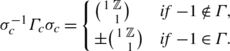
For the uniqueness of σ _c , let $\sigma_{c}'$ be another element of $\operatorname{GL}_{2}^{+}(\mathbb{Q})$ with the same properties. Let $g=\sigma_{c}^{-1}\sigma_{c}'$, so $\sigma_{c}'=\sigma_{c}g$. The first property implies g∞=∞, so is an upper triangular matrix. Consider the case −1∉Γ. The second property implies . In particular, one gets , which implies the claim. The case −1∈Γ is similar. □

Definition 2.6.4

Let Γ be a subgroup of finite index in SL₂(ℤ). A meromorphic function f on ℍ is called weakly modular of weight k with respect to Γ, if f| _k γ=f holds for every γ∈Γ.

A weakly modular function f is called modular if for every cusp c∈ℚ∪{∞} there exists T _c >0 and some N _c ∈ℕ such that

$$f|\sigma_c(z) = \sum_{n\ge-N_c}a_{c,n} e^{2\pi inz} $$

holds for every z∈ℍ with $\operatorname{Im}(z)>T_{c}$. In other words this means that the Fourier expansion is bounded below at every cusp. One also expresses this by saying that f is meromorphic at every cusp. By Lemma 2.6.3 this condition does not depend on the choice of the element σ _c , whereas the Fourier coefficients do depend on this choice.

The function f is called a modular form of weight k for the group Γ, if f is modular and holomorphic everywhere, including the cusps, which means that a _c,n =0 for n<0 at every cusp c. A modular form is called a cusp form if the zeroth Fourier coefficients a _c,0 vanish for all cusps c. The vector spaces of modular forms and cusp forms are denoted by $\mathcal{M}_{k}(\varGamma )$ and S _k (Γ).

As already mentioned in the proof of Theorem 2.5.16, the Petersson inner product can be defined for cusp forms of any congruence group Γ as follows: for f,g∈S _k (Γ) one sets

$$\langle f,g\rangle_{\operatorname{Pet}}= \frac{1}{[\overline{\varGamma}(1):\overline{\varGamma}]}\int_{\varGamma \backslash \mathbb{H}}f(z) \overline{g(z)}y^k\frac{dx\,dy}{y^2}. $$

2.7 Non-holomorphic Eisenstein Series

In the theory of automorphic forms one also considers non-holomorphic functions of the upper half plane, besides the holomorphic ones. These so-called Maaß wave forms will be introduced properly in the next section. In this section, we start with a special example, the non-holomorphic Eisenstein series. We introduce a fact, known as the Rankin–Selberg method, which says that the inner product of a non-holomorphic Eisenstein series and a Γ ₀-automorphic function equals the Mellin integral transform of the zeroth Fourier coefficient of the automorphic function. This in particular implies that the Eisenstein series is orthogonal to the space of cusp forms, a fact of central importance in the spectral theory of automorphic forms.

Definition 2.7.1

The non-holomorphic Eisenstein series for Γ ₀=SL₂(ℤ) is for z=x+iy∈ℍ and s∈ℂ defined by

By Lemma 1.2.1 the series E(z,s) converges locally uniformly in $\mathbb{H}\times\{\operatorname{Re}(s)>1\}$. Therefore the Eisenstein series is a continuous function, holomorphic in s, by the convergence theorem of Weierstrass.

Definition 2.7.2

By a smooth function we mean an infinitely often differentiable function.

Lemma 2.7.3

For fixed s with $\operatorname{Re}(s)>2$ the Eisenstein series E(z,s) is a smooth function in z∈ℍ.

Proof

We divide the sum that defines E(z,s) into two parts. One part with m=0 and the other with m≠0. For m=0 the sum does not depend on z, so the claim follows trivially. Consider the case m≠0 and let log be the principal branch of the logarithm, i.e. it is defined on ℂ∖(−∞,0] by log(re ^iθ)=log(r)+iθ, if r>0 and −π<θ<π. For z∈ℍ and $w\in\overline{\mathbb{H}}$, the lower half plane, we have

$$\log(zw)=\log(z)+\log(w). $$

For m≠0, n∈ℤ, and z∈ℍ, one of the two complex numbers mz+n, $m\bar{z}+n$ is in ℍ, the other in $\overline{\mathbb{H}}$. Hence

$$|mz+n|^{-2s} = e^{-s\log((mz+n)(m\bar{z}+n))} = e^{-s\log (mz+n)}e^{-s\log(m\bar{z}+n)}. $$

Write log(mz+n)=log(|mz+n|)+iθ for some |θ|<π. Then

so that

$$\bigl \vert e^{-s\log(mz+n)}\bigr \vert = e^{\operatorname{Re}(-s\log (mz+n))}\le e^{|\operatorname{Im}(s)|\pi} |mz+n|^{-\operatorname{Re}(s)}. $$

For z∈ℍ and $w\in\overline{\mathbb{H}}$ define

Keep w fixed and estimate the summand of the series F(z,w,s) as follows

$$\big|e^{-s\log(mz+n)}e^{-s\log(mw+n)}\big| \le Ce^{2|\operatorname {Im}(s)|\pi }|mz+n|^{-\operatorname{Re}(s)}, $$

with a constant C>0, which depends on w. According to Lemma 1.2.1, the series F(z,w,s) converges locally uniformly in z, for fixed w and s with $\operatorname{Re}(s)>2$. As the summands are holomorphic, the function F(z,w,s) is holomorphic in z. The same argument shows that F is holomorphic in w for fixed z. By Exercise 2.20 the function F(z,w,s) can locally be written as a power series in z and w simultaneously, which means that F(z,w,s) is a smooth function in (z,w) for fixed s with $\operatorname{Re} (s)>2$. Therefore $F(z,\overline{z},s) = E(z,s)$ is a smooth function, too. □

Lemma 2.7.4

Let Γ ₀=SL₂(ℤ) and let Γ _0,∞ be the stabilizer group of ∞, so . Then the map

is a bijection.

Proof

If c,d∈ℤ are coprime, then there exist a,b∈ℤ such that ad−bc=1. If (a,b) is one such pair, then every other is of the form (a+cx,b+dx) for some x∈ℤ. (Idea of proof: Assume 1<c≤d. After division with remainder there is 0≤r<c with d=r+cq. Then divide c by r with remainder and so on. This algorithm will stop. Plugging in the solutions backwards gives a pair (a,b).)

For and one has

$$\left(\matrix{1&x\cr& 1}\right) \left(\matrix{a&b\cr c&d}\right) = \left(\matrix{a+cx& b+dx\cr c&d}\right). $$

This implies the lemma. □

Definition 2.7.5

An automorphic function on ℍ with respect to the congruence subgroup Γ⊂SL₂(ℤ) is a function ϕ:ℍ→ℂ, which is invariant under the operation of Γ, so that ϕ(γz)=ϕ(z) holds for every γ∈Γ.

Proposition 2.7.6

• (a) The series $\tilde{E}(z,s) = \sum_{\gamma:\varGamma _{\infty}\backslash \varGamma }\operatorname{Im}(\gamma z)^{s}$ converges for $\operatorname {Re}(s)>1$ and we have

  $$E(z,s) = \pi^{-s}\varGamma (s)\zeta(2s)\tilde{E}(z,s), $$

  where ζ(s) is the Riemann zeta function.

• (b) The functions E(z,s) and $\tilde{E}(z,s)$ are automorphic under Γ=SL₂(ℤ), i.e. we have

  $$E(\gamma z,s) = E(z,s) $$

  for every γ∈Γ. The same holds for $\tilde{E}$.

Proof

(a) With we have $\operatorname {Im}(\gamma z)=\operatorname{Im}(z)/|cz+d|^{2}$. According to Lemma 2.7.4 it holds that

Hence we get convergence with E(z,s) as a majorant. We conclude

(b) It suffices to show the claim for $\tilde{E}$. We compute

$$\tilde{E}(\gamma z,s) = \sum_{\tau:\varGamma _\infty\backslash \varGamma }\operatorname{Im}( \tau \gamma z)^s = \sum_{\tau:\varGamma _\infty\backslash \varGamma } \operatorname{Im}(\tau z)^s, $$

since if τ runs through a set of representatives for Γ _∞∖Γ, then so does τγ. □

In particular it follows that

$$E(z+1,s) = E(z,s). $$

It follows that for $\operatorname{Re}(s)>2$ the smooth function E(z,s) has a Fourier expansion in z. We will examine this Fourier expansion more closely.

The integral

$$K_s(y) = \frac{1}{2}\int_0^\infty e^{-y(t+t^{-1})/2}t^s\frac{dt}{t} $$

converges locally uniformly absolutely for y>0 and s∈ℂ. The function K _s so defined is called the K-Bessel function. It satisfies the estimate

$$\big|K_s(y)\big| \le e^{-y/2} K_{\operatorname{Re}(s)}(2),\quad\mbox{if } y>4. $$

Proof

For two real numbers a,b we have

$$a>b>2\quad \Rightarrow\quad \left \{ \begin{array}{c}ab>2a\\ 2a>a+b \end{array} \right \}\ \quad \Rightarrow\quad ab>a+b. $$

The last assertion is symmetric in a and b, so it holds for all a,b>2. Therefore one has e ^−ab<e ^−a e ^−b. Applying this to a=y/2>2 and b=t+t ⁻¹ and integrating along t gives

$$\big|K_s(y)\big| \le \frac{1}{2}\int_0^\infty e^{-y/2}e^{-(t+t^{-1})}t^{\operatorname{Re} (s)}\frac{dt}{t} = e^{-y/2} K_{\operatorname{Re}(s)}(2). $$

We also note that the integrand in the Bessel integral is invariant under t↦t ⁻¹, s↦−s, so that

$$K_{-s}(y) = K_s(y). $$

Theorem 2.7.7

The Eisenstein series E(z,s) has a Fourier expansion

$$E(z,s) = \sum_{r=-\infty}^\infty a_r(y,s)e^{2\pi irx}, $$

where

$$a_0(y,s) = \pi^{-s}\varGamma (s)\zeta(2s) y^s+\pi^{s-1}\varGamma (1-s)\zeta (2-2s) y^{1-s} $$

and for r≠0,

$$a_r(y,s) = 2|r|^{2-1/2}\sigma_{1-2s}\bigl(|r|\bigr)\sqrt{y} K_{s-\frac{1}{2}}\bigl(2\pi|r|y\bigr). $$

One reads off that the Eisenstein series E(z,s), as a function in s, has a meromorphic expansion to all of ℂ. It is holomorphic except for simple poles at s=0,1. It is a smooth function in z for all s≠0,1. Every derivative in z is holomorphic in s≠0,1. The residue at s=1 is constant in z and takes the value 1/2. The Eisenstein series satisfies the functional equation

$$E(z,s) = E(z,1-s). $$

Locally uniformly in x∈ℝ one has

$$E(x+iy) = O\bigl(y^{\sigma}\bigr),\quad\mbox{for } y\to\infty, $$

where $\sigma=\max(\operatorname{Re}(s),1-\operatorname{Re}(s))$.

Proof

The claims all follow from the explicit Fourier expansion, which remains to be shown.

Definition 2.7.8

A function f:ℝ→ℂ is called a Schwartz function if f is infinitely differentiable and every derivative f ^(k), k≥0 is rapidly decreasing. Let $\mathcal{S}(\mathbb{R})$ denote the vector space of all Schwartz functions on ℝ. If f is in $\mathcal{S}(\mathbb{R})$, then its Fourier transform $\hat{f}$ also lies in $\mathcal{S}(\mathbb{R})$; see [Dei05, Rud87, SW71].

Lemma 2.7.9

If $\operatorname{Re}(s)>\frac{1}{2}$ and r∈ℝ, then

Proof

We plug in the Γ-integral on the left-hand side to get

$$\int_\mathbb{R}\int_0^\infty e^{-t}\biggl(\frac{ty}{\pi (x^2+y^2)}\biggr)^se^{2\pi irx} \frac{dt}{t}\,dx = \int_0^\infty\!\!\int _\mathbb{R}e^{-\pi t(x^2+y^2)/y}t^se^{2\pi irx}\, dx\, \frac{dt}{t}, $$

where we have substituted t↦πt(x ²+y ²)/y. The function $f(x)=e^{-\pi x^{2}}$ is its own Fourier transform: $\hat{f}=f$. To see this, note that f is, up to scaling, uniquely determined as the solution of the differential equation

$$f'(x) = -2\pi x f(x). $$

By induction one shows that for every natural n there is a polynomial p _n (x), such that $f^{(n)}(x)=p_{n}(x)e^{-\pi x^{2}}$. So f lies in the Schwartz space $\mathcal{S}(\mathbb{R})$ and so does its Fourier transform $\hat{f}$, and one computes

$$(\hat{f})'(y) = \int_\mathbb{R}(-2\pi ix)e^{-\pi x^2}e^{-2\pi xy}\,dx = i\int_\mathbb{R} \bigl(e^{-\pi x^2}\bigr)'e^{-2\pi ixy}\,dx = -2\pi y\hat{f}(y). $$

Therefore $\hat{f}=c f$ and $\skew{7}\hat{\hat{f}}=c\hat{f}= c^{2} f$. Since, on the other hand, $\skew{7}\hat{\hat{f}}(x)=f(-x)=f(x)$, we infer that c ²=1, so c=±1. By $\hat{f}(0)=\int_{\mathbb{R}}e^{-\pi x^{2}}\,dx>0$ it follows that c=1.

By a simple substitution one gets from this

$$\int_\mathbb{R}e^{-t\pi x^2/y}e^{2\pi irx}\,dx = \sqrt{ \frac{y}{t}} e^{-y\pi r^2/t}. $$

We see that the left-hand side of the lemma equals

$$\int_0^\infty e^{-\pi ty}\sqrt{\frac{y}{t}} e^{-y\pi r^2/t} t^s \frac{dt}{t}, $$

which gives the claim. □

We now compute the Fourier expansion of the Eisenstein series E(z,s). The coefficients are given by

The summands with m=0 only give a contribution in the case r=0. This contribution is

$$\pi^{-s}\varGamma (s) y^s\sum _{n=1}^\infty n^{-2s} = \pi^{-s} \varGamma (s)\zeta (2s) y^s. $$

For m≠0 note that the contribution for (m,n) and (−m,−n) are equal. Therefore it suffices to sum over m>0. The contribution to a _r is

The substitution x↦x−n/m yields

$$\pi^{-s}\varGamma (s) y^s\sum _{m=1}^\infty m^{-2s}\ \ \sum _{n\operatorname{mod} m}e^{2\pi irn/m} \int_{-\infty}^\infty \bigl(x^2+y^2\bigr)^{-s} e^{-2\pi irx}\,dx. $$

Because of

the contribution is

$$\pi^{-s}\varGamma (s) y^s\sum _{m|r} m^{1-2s} \int_{-\infty}^\infty \bigl(x^2+y^2\bigr)^{-s} e^{2\pi irx}\,dx. $$

There are two cases. Firstly, if r=0, the condition m|r is vacuous and we get

$$\pi^{-s}\varGamma (s) y^s\zeta(2s-1) \int _{-\infty}^\infty\bigl(x^2+y^2 \bigr)^{-s} \,dx = \pi^{-s+1/2}\varGamma \biggl(s-\frac{1}{2}\biggr) \zeta(2s-1)y^{1-s}, $$

where we have used Lemma 2.7.9. The Riemann zeta function satisfies the functional equation

$$\hat{\zeta}(s) = \hat{\zeta}(1-s), $$

with $\hat{\zeta}(s)=\pi^{-s/2}\varGamma (s/2)\zeta(s)$, as is shown in Theorem 6.1.3. Therefore the zeroth term a ₀ is as claimed. Secondly, in the case r≠0 we get the claim again by Lemma 2.7.9.  □

We now explain the Rankin–Selberg method. Let Γ=SL₂(ℤ) and let ϕ:ℍ→ℂ be a smooth, Γ-automorphic function. We assume that ϕ is rapidly decreasing at the cusp ∞, i.e. that

$$\phi(x+iy)=O\bigl(y^{-N}\bigr), \quad y\ge1 $$

holds for every N∈ℕ. Because of ϕ(z+1)=ϕ(z) the function ϕ has a Fourier expansion

$$\phi(z)=\sum_{n=-\infty}^\infty \phi_n(y)\,e^{2\pi inx} $$

with $\phi_{n}(y)=\int_{0}^{1}\phi(x+iy)\,e^{-2\pi inx}\,dx$. The term ϕ ₀ is called the constant term of the Fourier expansion. Let

$$\mathcal{M}\phi_0(s) = \int_0^\infty \phi_0(y) y^s\frac{dy}{y} $$

be the Mellin transform of the zeroth term. We shall show that this integral converges for $\operatorname{Re}(s)>0$. Put

$$\varLambda (s) = \pi^{-s}\varGamma (s)\zeta(2s)\mathcal{M} \phi_0(s-1). $$

Proposition 2.7.10

(Rankin–Selberg method)

The integral $\mathcal{M}\phi_{0}(s)$ converges locally uniformly absolutely in the domain $\operatorname{Re}(s)>0$. One has

$$\varLambda (s) = \int_{\varGamma (1)\backslash \mathbb{H}} E(z,s)\phi (z) \frac{dx\,dy}{y^2}. $$

The function Λ(s), defined for $\operatorname{Re}(s)>0$, extends to a meromorphic function on ℂ with at most simple poles at s=0 and s=1. It satisfies the functional equation

$$\varLambda (s) = \varLambda (1-s). $$

The residue at s=1 equals

$$\operatorname{res}_{s=1}\varLambda (s) = \frac{1}{2}\int _{\varGamma (1)\backslash \mathbb{H}}\phi(z)\frac{dx\,dy}{y^2}. $$

Proof

The proof relies on an unfolding trick as follows

The claims now follow from Theorem 2.7.7. □

We apply the Rankin–Selberg method to show that the Rankin–Selberg convolution of modular L-functions is meromorphic. Let k∈2ℕ₀ and let $f,g\in\mathcal{M}_{k}$ be normalized Hecke eigenforms. Denote the Fourier coefficients of f and g by a _n and b _n for n≥0, respectively. We define the Rankin–Selberg convolution of L(f,s) and L(g,s) by

$$L(f\times g,s)\stackrel{\mathrm{def}}{=}\zeta(2s-2k+2)\sum _{n=1}^\infty a_nb_nn^{-s}. $$

By Proposition 2.3.1 and Theorem 2.3.2 one has a _n ,b _n =O(n ^k−1). Therefore the series L(f×g,s) converges absolutely for $\operatorname{Re}(s)>2k-1$. We put

$$\varLambda (f\times g,s) = (2\pi)^{-2s}\varGamma (s)\varGamma (s-k+1)L(f\times g,s). $$

Theorem 2.7.11

Suppose that one of the functions f,g is a cusp form. Then Λ(f×g,s) extends to a meromorphic function on ℂ. It is holomorphic except for possible simple poles at s=k and s=k−1. It satisfies the functional equation

$$\varLambda (f\times g,s) = \varLambda (f\times g,2k-1-s). $$

The residue at s=k is $\frac{1}{2}\pi^{1-k}{\langle f,g\rangle}_{k}$.

Proof

We apply Proposition 2.7.10 to the function $\phi(z)=f(z)\overline{g(z)}y^{k}$. Then

Since $\int_{0}^{1}e^{2\pi i(n-m)x}\,dx=0$ except for n=m, we get $\phi_{0}(y) = \sum_{n=1}^{\infty}a_{n}\overline{b_{n}}e^{-4\pi ny}y^{k}$. So

The number b _n is the eigenvalue of the Hecke operator T _n . As T _n is self-adjoint, b _n is real. Therefore,

$$\mathcal{M}\phi_0(s-1) = (4\pi)^{-s-k+1}\varGamma (s-1+k) \frac{1}{\zeta (2s)}L(f\times g,s-1+k). $$

Let Λ(s) be as in Proposition 2.7.10. It follows that

$$\varLambda (s) = 4^{-s-k+1}\pi^{-2s-k+1}\varGamma (s)\varGamma (s-1+k) L(f\times g,s-1+k), $$

or

$$\varLambda (s+1-k) = \pi^{k-1}(2\pi)^{-2s}\varGamma (s) \varGamma (s+1-k) L(f\times g,s) = \pi^{k-1}\varLambda (f\times g,s). $$

By Proposition 2.7.10 one has Λ(s+1−k)=Λ(1−(s+1−k)), which implies the claimed functional equation. Finally one has

 □

Next we show that the L-function L(f×g,s) has an Euler product. We factorize the polynomials

Theorem 2.7.12

Let k∈2ℕ₀ and let $f,g\in\mathcal{M}_{k}$ be normalized Hecke eigenforms. The Rankin–Selberg L-function has the Euler product expansion

$$L(f\times g,s) = \prod_{p}\prod _{i=1}^2\prod_{j=1}^2 \bigl(1-\alpha_i(p)\beta_j(p)p^{-s} \bigr)^{-1}. $$

Proof

This is a consequence of the following lemma.

Lemma 2.7.13

Let α ₁,α ₂,β ₁,β ₂ be complex numbers with α ₁ α ₂ β ₁ β ₂≠0 and suppose that the equalities

hold for small complex numbers z. Then for small z one has

$$\sum_{r=0}^\infty a_rb_r z^r = \bigl(1-\alpha_1\alpha_2 \beta_1\beta_2 z^2\bigr)\prod _{i=1}^2\prod_{j=1}^2(1- \alpha_i\beta_j z)^{-1}. $$

Proof

Let $\phi(z)=\sum_{r=0}^{\infty}a_{r}z^{r}$ and $\psi(z)=\sum_{r=0}^{\infty}b_{r}z^{r}$. Consider the path integral

$$\frac{1}{2\pi i}\int_{\partial K}\phi(qz)\psi\bigl(q^{-1} \bigr)\frac{dq}{q}, $$

where K is a circle around zero such that the poles of q↦ϕ(zq) are outside K, and the poles of q↦ψ(q ⁻¹) are inside. This is possible for z small enough. The integral is equal to

$$\sum_{r,r'=0}^\infty a_rb_{r'} x^r\ \frac{1}{2\pi i}\int_{\partial K}q^{r-r'-1} \,dq = \sum_{r=0}^\infty a_rb_r x^r. $$

On the other hand, the integral equals

$$\frac{1}{2\pi i}\int_{\partial K}\frac{1}{(1-\alpha_1xq) (1-\alpha_2xq) (1-\beta_1q^{-1}) (1-\beta_2q^{-1})}\frac{dq}{q}, $$

which we calculate by the residue theorem as

$$\bigl(1-\alpha_1\alpha_2\beta_1 \beta_2 x^2\bigr)\prod_{i=1}^2 \prod_{j=1}^2(1-\alpha_i \beta_j x)^{-1}. $$

 □

2.8 Maaß Wave Forms

This section is not strictly necessary for the rest of the book, but we include it for completeness. In this section we shall not give full proofs all the time, but rather sketch the arguments.

The group G=SL₂(ℝ) acts on ℍ by diffeomorphisms, so it acts on C ^∞(ℍ) by L _g :C ^∞(ℍ)→C ^∞(ℍ), where for g∈G the operator L _g is defined by

$$L_g\varphi (z) = \varphi \bigl(g^{-1}z\bigr). $$

On the upper half plane ℍ we have the hyperbolic Laplace operator, which is a differential operator defined by

$$\varDelta = -y^2\biggl(\frac{\partial^2}{\partial x^2}+\frac{\partial^2}{\partial y^2}\biggr). $$

Lemma 2.8.1

The hyperbolic Laplacian is invariant under G, i.e. one has

$$L_g\varDelta L_{g^{-1}} = \varDelta $$

for every g∈G.

Proof

The assertion is equivalent to L _g Δ=ΔL _g . It suffices to show this assertion for generators of the group SL₂(ℝ). Such generators are given in Exercise 2.6. We leave the explicit calculation for this invariance to the reader, see Exercise 2.7. □

Definition 2.8.2

A Maaß wave form or Maaß form for the group Γ(1) is a smooth function f on ℍ such that

• f(γz)=f(z) for every γ∈Γ(1),

• Δf=λf for some λ∈ℂ,

• there exists N∈ℕ with f(x+iy)=O(y ^N) for y≥1.

If additionally one has

$$\int_0^1 f(z+t)\,dt = 0 $$

for every z∈ℍ, then f is called a Maaß cusp form.

Proposition 2.8.3

The non-holomorphic Eisenstein series

is a Maaß form; more precisely it holds that

$$\varDelta E(z,s) = s(1-s)E(z,s),\quad s\ne0,1. $$

Proof

We only have to show the eigen-equation. We have

$$E(z,s) = \pi^{-s}\varGamma (s)\zeta(2s)\tilde{E}(z,s) $$

with $\tilde{E}(z,s) = \sum_{\varGamma _{\infty}\backslash \varGamma }\operatorname{Im}(\gamma z)^{s}$. So it suffices to show the eigen-equation for $\tilde{E}$. We have

$$\varDelta \bigl(y^s\bigr) = - y^2\biggl( \frac{\partial^2}{\partial x^2}+\frac{\partial^2}{\partial y^2}\biggr)y^s = s(1-s)y^s. $$

By invariance of the Laplace operator we get

$$\varDelta \operatorname{Im}(\gamma z)^s = s(1-s)\operatorname{Im}( \gamma z)^s $$

for every γ∈Γ. By means of Lemma 1.2.1 one shows that for $\operatorname{Re}(s)>3$ the series $\sum_{\varGamma _{\infty}\backslash \varGamma }\frac{\partial }{\partial y}\operatorname{Im}(z)^{s}$ and $\sum_{\varGamma _{\infty}\backslash \varGamma }\frac {\partial^{2}}{\partial y^{2}}\operatorname{Im}(z)^{s}$ as well as the x-derivatives converge locally uniformly, so we may differentiate the Eisenstein series term-wise. This implies the claim for $\tilde{E}$ and therefore also for E in the domain $\operatorname{Re}(s)>3$. For arbitrary s∈ℂ the Fourier expansion shows that ΔE(z,s)−s(1−s)E(z,s) is a meromorphic function in s, which for $\operatorname{Re}(s)>3$ is constantly equal to zero. By the identity theorem it is zero everywhere. □

The differential equation can also be expressed in the form

$$\varDelta E\biggl(z,\nu+\frac{1}{2}\biggr) = \biggl(\frac{1}{4}-\nu^2\biggr) E \biggl(z,\nu+\frac{1}{2}\biggr). $$

Let f be an arbitrary Maaß form for the group Γ(1). Because of f(z+1)=f(z) the function f has a Fourier expansion

$$f(x+iy) = \sum_{r=-\infty}^\infty a_r(y)e^{2\pi irx}. $$

Lemma 2.8.4

Let λ∈ℂ be the Laplace eigenvalue of the Maaß form f. There is a ν∈ℂ, which is unique up to sign, such that $\lambda= \frac{1}{4}-\nu^{2}$. The Fourier coefficients of f are

$$a_r(y) = a_r \sqrt{y} K_\nu\bigl(2\pi|r|y\bigr) $$

if r≠0, where a _r ∈ℂ depends only on r. For r=0 one has

$$a_0(y) = a_0 y^{\frac{1}{2}-\nu}+b_0y^{\frac{1}{2}+\nu} $$

for some a ₀,b ₀∈ℂ.

Proof

We have $\varDelta f=(\frac{1}{4}-\nu^{2})f(z)$. The definition of a _r (y),

$$a_r(y) = \int_0^1 f(x+iy) e^{-2\pi irx}\,dx, $$

implies

So there is a differential equation of second order,

$$y^2\frac{\partial^2}{\partial y^2}a_r(y) +\biggl(\frac{1}{4}- \nu^2-4\pi r^2y^2\biggr)a_r(y) = 0. $$

The rth Fourier coefficient of the Eisenstein series is a solution of this differential equation. Therefore the function

$$a_r(y) = \sqrt{y} K_\nu\bigl(2\pi|r|y\bigr) $$

solves this linear differential equation. A second solution is given by

$$b_r(y) = \sqrt{y} I_\nu\bigl(2\pi|r|y\bigr), $$

where I _ν is the I-Bessel function [AS64]. As the differential equation is linear of order 2, every solution is a linear combination of these two basis solutions. A proof of this classical fact can be found for example in [Rob10]. Further, the I-Bessel function grows exponentially, whereas the K-Bessel function decreases exponentially [AS64]. According to the definition of a Maaß form, the function a _r (y) can only grow moderately, and the claim follows. □

Let ι:ℍ→ℍ be the anti-holomorphic map $\iota(z)=-\overline{z}$, so ι(x+iy)=−x+iy. Then $\iota\circ\iota=\operatorname{Id}_{\mathbb{H}}$ and one finds that ι commutes with the hyperbolic Laplacian Δ, when ι acts on functions f of the upper half plane by $\iota(f)(z)\stackrel{\mathrm{def}}{=}f(\iota(z))$. Therefore ι maps the λ-eigenspace into itself for every λ∈ℂ. By $\iota^{2}=\operatorname{Id}$ the map ι itself has at most the eigenvalues ±1. A Maaß form f is called an even Maaß form if ι(f)=f and an odd Maaß form if ι(f)=−f. By

$$f=\frac{1}{2}\bigl(f+\iota(f)\bigr)+\frac{1}{2}\bigl(f-\iota(f)\bigr) $$

every Maaß form is the sum of an even and an odd Maaß form.

Theorem 2.8.5

Let

$$f(z) = \sum_{r\ne0}a_r \sqrt{y} K_\nu\bigl(2\pi|r|y\bigr) e^{2\pi irx} $$

be a Maaß cusp form and let

$$L(s,f) = \sum_{n=1}^\infty a_nn^{-s} $$

be the corresponding L-series. The series L(s,f) converges for $\operatorname{Re}(s)>3/2$ and extends to an entire function on ℂ. Let f be even or odd and let ε=0 if f is even and ε=1 if f is odd. Let $\varDelta f=(\frac{1}{4}-\nu^{2})f$. Then with

$$\varLambda (s,f) = \pi^{-s}\varGamma \biggl(\frac{s-\varepsilon +\nu }{2}\biggr) \varGamma \biggl(\frac{s-\varepsilon -\nu}{2}\biggr)L(s,f), $$

one has the functional equation

$$\varLambda (s,f) = (-1)^\varepsilon \varLambda (1-s,f). $$

Proof

Note that a _−r =(−1)^ε a _r holds. The convergence is clear by the following lemma.

Lemma 2.8.6

We have a _n =O(n ^1/2).

Proof

There are C,N>0 such that for y>1 the inequality |f(x+iy)|≤Cy ^N holds. If y<1/2 and if w∈D is conjugate to z modulo Γ(1), then $\operatorname{Im}(w)\le\frac{1}{y}$. So suppose y<1/2. Then it follows that |f(x+iy)|≤Cy ^−N. So that for y<1/2 one has

$$|a_r|\sqrt{y}\big|K_s\bigl(2\pi|r|y\bigr)\big|\le\int _0^1\big|f(x+iy)\big|\,dx\le Cy^{-N}. $$

With y=1/|r| we get from this

$$|a_r|\le C r^{N+\frac{1}{2}}\big|K_s(2 \pi)\big|^{-1}. $$

As the K-Bessel function is rapidly decreasing and f is a cusp form, we conclude that f is bounded on D and therefore on ℍ. This argument can be repeated with N=0. The claim is proven. □

Lemma 2.8.7

The integral

$$\int_0^\infty K_\nu(y) y^s\frac{dy}{y} = 2^{s-2}\varGamma \biggl( \frac{s+\nu }{2}\biggr)\varGamma \biggl(\frac{s-\nu}{2}\biggr) $$

converges absolutely if $\operatorname{Re}(s)>|\operatorname{Re}(\nu)|$.

Proof

Plugging in the definition of K _ν , the left-hand side becomes

$$\frac{1}{2} \int_0^\infty\!\!\int_0^\infty e^{-(t+t^{-1})y/2}t^\nu y^s\frac {dy}{y} \frac{dt}{t}. $$

We use the change of variables rule with the diffeomorphism ϕ:(0,∞)×(0,∞)→(0,∞)×(0,∞) given by

$$\phi(t,y) = \biggl(\frac{1}{2}ty,\frac{1}{2}t^{-1}y\biggr) = (u,v). $$

Then $y=2\sqrt{uv}$ and $t=\sqrt{u/v}$. The Jacobian matrix of ϕ is

$$D\phi(t,y) = \frac{1}{2} \left(\matrix{y&t\cr{-\frac{y}{t^2}}& {\frac{1}{t}}}\right). $$

Its determinant equals $\det D\phi=\frac{y}{2t}$. By the change of variables rule the integral equals

$$2^{s-1}\int_0^\infty\!\!\int _0^\infty e^{-u-v}v^{(s-\nu)/2}u^{(s+\nu)/2} \frac{du}{u}\frac{dv}{v}. $$

The claim follows. □

We now prove the theorem in the case when f is even. Then

$$\int_0^\infty f(iy)y^{s-1/2} \frac{dy}{y} = \frac{1}{2}\varLambda (s,f). $$

By Lemma 2.8.6 we infer that f(iy) is rapidly decreasing for y→∞. Because of $f(iy)=f(i\frac{1}{y})$ the claim follows similar to Theorem 2.4.5.

If f is odd, put

$$g(z) = \frac{1}{4\pi i}\frac{\partial f}{\partial x}(z) = \sum_{n=1}^\infty a_nn\sqrt{y} K_\nu(2\pi ny)\cos(2\pi nx). $$

Then

$$\int_0^\infty g(iy)y^{s+1/2} \frac{dy}{y} = \varLambda (s,f). $$

Because of $g(iy)=-\frac{1}{y^{2}}g(\frac{i}{y})$ the claim follows in this case as well.  □

More generally, for every k∈ℤ we introduce the operator

$$\varDelta _k = -y^2\biggl(\frac{\partial^2}{\partial x^2}+ \frac{\partial^2}{\partial y^2}\biggr)+iky\frac{\partial}{\partial x}. $$

A computation shows that

$$\varDelta _k = -L_{k+2}R_k-\frac{k}{2}\biggl(1+\frac{k}{2}\biggr) = -R_{k-2}L_k+\frac{k}{2}\biggl(1-\frac{k}{2}\biggr), $$

where

$$R_k = iy\frac{\partial}{\partial x}+y\frac{\partial}{\partial y}+ \frac{k}{2},\qquad L_k = -iy\frac{\partial}{\partial x}+y\frac{\partial}{\partial y}-\frac{k}{2}. $$

Definition 2.8.8

For f∈C ^∞(ℍ) and let

$$f||_kg(z) = \biggl(\frac{cz+d}{|cz+d|}\biggr)^{-k}f(gz) = \biggl(\frac{c\overline{z}+d}{|cz+d|}\biggr)^{k}f(gz). $$

Lemma 2.8.9

With f∈C ^∞(ℍ) and g∈G=SL₂(ℝ) we have

$$(R_kf)||_{k+2}g = R_k(f||_kg), \qquad(L_kf)||_{k-2}g = L_k(f||_kg) $$

and

$$(\varDelta _kf)||_kg = \varDelta _k(f||_k g). $$

Proof

A direct computation verifies the first two identities. The third then follows. Alternatively, one waits until the next section, where a Lie-theoretic and more structural proof is given. □

Differential operators are naturally defined on infinite-dimensional spaces like C ^∞(ℝ). These are not Hilbert spaces, but one can define differential operators on dense subspaces of natural Hilbert spaces. This motivates the next definition.

Definition 2.8.10

Let H be a Hilbert space. By an operator on H we mean a pair (D _T ,T), where D _T ⊂H is a linear subspace of H and T:D _T →H is a linear map. The space D _T is the domain of the operator. The operator is said to be densely defined if D _T is dense in H. The operator is called a closed operator if its graph G(T)={(h,T(h)):h∈D _T } is a closed subset of H×H.

An operator T is called symmetric if

$$\bigl\langle T(v),w\bigr\rangle = \bigl\langle v,T(w)\bigr\rangle $$

holds for all v,w∈D _T .

Given a densely defined operator T on H we define its adjoint operator T ^∗ as follows. Firstly the domain $D_{T^{*}}$ is defined to be the set of all v∈H, for which the map w↦〈Tw,v〉 is a bounded linear map on D _T . As D _T is dense, this map extends uniquely to a continuous linear map on H. By the Riesz Representation Theorem there exists a uniquely determined vector T ^∗ v∈H, such that 〈Tw,v〉=〈w,T ^∗ v〉 holds for every w∈D _T . It is easy to see that the so-defined map $T^{*}:D_{T^{*}}\to H$ is linear. If the domain $D_{T^{*}}$ is dense, one can show that the adjoint operator T ^∗ is closed.

An operator T is called self-adjoint if $D_{T^{*}}=D_{T}$ and T ^∗=T. We have

$$T \mbox{ self-adjoint}\quad \Rightarrow\quad T\mbox{ closed and symmetric}, $$

but the converse is false in general, as the following example shows.

Example 2.8.11

Let H=L ²([0,1]) and let D _T be the set of all continuous functions f on [0,1] of the form $f(x)=\int_{0}^{x}f'(t)\,dt = \langle f',\mathbf{1}_{[0,x]}\rangle$ for some f′∈L ²(0,1) with f′⊥1 _[0,1]. Then f is uniquely determined by f. For every f∈D _T one has f(0)=0=f(1). Let T be the operator with domain D _T given by

$$T(f) = f'. $$

Since C([0,1]) is dense in H, for every f∈D _T there is a sequence of continuously differentiable functions f _j with f _j →f and Tf _j →Tf. Using integration by parts we get

$$\langle Tf,g\rangle = \langle f,Tg\rangle $$

for all f,g∈D _T . This means that T is indeed symmetric. It is also closed, since for every sequence f _j ∈D _T with f _j →f and Tf _j →g we have f∈D _T and g=Tf. It remains to show that T ^∗≠T. The constant function 1, for example, lies in $D_{T^{*}}$, but not in D _T . Furthermore, the adjoint operator T ^∗ is not symmetric.

If H is finite-dimensional, then every densely defined operator T is defined on all of H, as the only dense subspace is H itself.

We recall from linear algebra:

Theorem 2.8.12

(Spectral theorem)

Let T:H→H be a self-adjoint operator on a finite-dimensional Hilbert space H. Then H is a direct sum of eigenspaces,

$$H = \bigoplus_{\lambda\in\mathbb{R}}\operatorname{Eig}(T,\lambda), $$

where

$$\operatorname{Eig}(T,\lambda) = \bigl\{ v\in H: T(v) = \lambda v\bigr\}. $$

The proof is part of a linear algebra lecture. If H is infinite-dimensional, there is also a spectral theorem for self-adjoint operators. However, the space is not a direct sum in general, but a so-called direct integral of eigenspaces. We shall come back to this later.

Definition 2.8.13

The support of a function f:X→ℂ on a topological space X is the closure of the set {x∈X:f(x)≠0}. By C _c (X) we denote the set of all continuous functions of compact support.

As usual, we denote by L ²(ℍ) the space of all measurable functions f:ℍ→ℂ such that ∫_ℍ|f(z)|² dμ(z)<∞ modulo the subspace of all functions vanishing outside a set of measure zero. The measure μ is the invariant measure $\frac{dx\,dy}{y^{2}}$. The space $D=C_{c}^{\infty}(\mathbb{H})$ of all infinitely differentiable functions on ℍ of compact support is a dense subspace on which the operator Δ _k is defined.

Proposition 2.8.14

The operator Δ _k with domain $C_{c}^{\infty}(\mathbb{H})$ is a symmetric operator on the Hilbert space H=L ²(ℍ).

Proof

Let

$$\varDelta ^e = \frac{\partial^2}{\partial x^2}+ \frac{\partial^2}{\partial y^2} $$

be the Euclidean Laplace operator and let d denote the exterior differential, which maps n-differential forms to (n+1)-forms. For $f,g\in C_{c}^{\infty}(\mathbb{H})$ we have

$$d\biggl(g\biggl(\frac{\partial f}{\partial x}dy-\frac{\partial f}{\partial y}dx\biggr)-f\biggl( \frac{\partial g}{\partial x}dy-\frac{\partial g}{\partial y}dx\biggr)\biggr) = \bigl(g \varDelta ^ef-f\varDelta ^e g\bigr)\, dx\wedge dy. $$

By Stokes’s integral theorem we conclude

$$\int_\mathbb{H}\bigl(\overline{g}\varDelta ^e f-f \varDelta ^e\overline{g}\bigr)\, dx\wedge dy = 0, $$

so

$$\int_\mathbb{H}\overline{g}\varDelta ^e f\, dx\wedge dy = \int_\mathbb {H}f\varDelta ^e\overline{g}\, dx\wedge dy. $$

Write $T=\frac{i}{y}\frac{\partial}{\partial x}$. Integration by parts yields

where Ω is any relatively compact open subset of ℍ with smooth boundary, containing the support of $f\overline{g}$. So

$$\int_\mathbb{H}(Tf)\overline{g}\, dx\wedge dy = \int _\mathbb {H}f(\overline{Tg})\, dx\wedge dy. $$

One has

$$\langle \varDelta _k f,g\rangle = \int_\mathbb{H}( \varDelta _kf)\overline{g}\frac{dx\wedge dy}{y^2} = \int_\mathbb{H} \bigl(-\varDelta ^e f+kTf\bigr)\overline{g}\, dx\wedge dy. $$

Hence the operator Δ _k is symmetric. □

Pick a discrete subgroup Γ of SL₂(ℝ). By invariance, the operator Δ _k preserves the set of all smooth functions f on ℍ, which satisfy f|| _k γ=f for every γ∈Γ. Write C ^∞(Γ∖ℍ,k) for the vector space of all these functions and L ²(Γ∖ℍ,k) for the space of all measurable functions f on ℍ with f|| _k γ=f for every γ∈Γ and

$$\big\|f^2\big\|\stackrel{\mathrm{def}}{=}\int_{\varGamma \backslash \mathbb {H}}\big|f(z)\big|^2 \frac{dx\,dy}{y^2} < \infty, $$

modulo the subspace of functions with ∥f∥=0. Note that the integral is well defined, since the function |f(z)|² is invariant under Γ. Then L ²(Γ∖ℍ,k) is a Hilbert space with inner product

$$\langle f,g\rangle = \int_{\varGamma \backslash \mathbb{H}} f(z)\overline{g(z)} \frac{dx\wedge dy}{y^2}. $$

For the rest of this section we assume that the topological space Γ∖ℍ is compact. This is equivalent to the quotient Γ∖SL₂(ℝ) being compact.

In that case one calls Γ a cocompact subgroup of SL₂(ℝ). A subgroup of SL₂(ℤ) is never cocompact, because SL₂(ℤ) is not cocompact itself. Do cocompact groups exist at all? Yes they do, and we will show this, using some facts of complex analysis, topology and elementary number theory.

• We start with a concrete example. Pick two rationals 0<p,q∈ℚ. The matrices

  $$i=\left(\matrix{\sqrt{p}& \cr& -\sqrt{p}}\right),\qquad j= \left(\matrix{&\sqrt{q}\cr\sqrt{q}&}\right) $$

  generate a ℚ-subalgebra M of M₂(ℝ) with the relations

  $$i^2=p,\qquad j^2=q,\qquad ij=-ji. $$

  These relations imply that the vectors 1,i,j,ij form a basis of M over ℚ, so M has dimension four over ℚ. The algebra M is a special case of a quaternion algebra.

  We now insist that p and q are prime numbers and that q is not quadratic modulo p, i.e. we assume that $q\not\equiv k^{2}\operatorname{mod} p$ for every number k modulo p. In that case one can show (Exercise 2.21), that M is a division algebra, which means that every m≠0 in M is invertible. The set

  $$M_\mathbb{Z}= \mathbb{Z}1\oplus\mathbb{Z}i\oplus\mathbb{Z}j\oplus \mathbb{Z}ij $$

  is a subring. Let

  $$\varGamma =\bigl\{\gamma\in M_\mathbb{Z}:\det(\gamma)=1\bigr\}. $$

  One can show that Γ is a discrete subgroup of SL₂(ℝ), such that Γ∖ℍ is compact.

• Let X be a Riemann surface of genus g≥0. Let $\tilde{X}$ be its universal covering and Γ its fundamental group, which we consider as a group of biholomorphic maps on $\tilde{X}$. Then there is a natural identification $\varGamma \backslash \tilde{X}\cong X$. The Riemann surface $\tilde{X}$ is simply connected and Γ acts on $\tilde{X}$ without fixed points. By the Riemann mapping theorem, there are the following possibilities:

  • (a) $\tilde{X}\cong\mathbb{P}_{1}(\mathbb{C})=\widehat{\mathbb{C}}$ the Riemann number sphere,

  • (b) $\tilde{X}\cong\mathbb{C}$,

  • (c) $\tilde{X}\cong\mathbb{H}$.

  In case (a) every biholomorphic map $\gamma:\tilde{X}\to\tilde{X}$ is a linear fractional $\gamma(z)=\frac{az+b}{cz+d}$ and every such transformation has at least one fixed point in $\widehat{\mathbb{C}}$, which means that Γ={1} and $X=\tilde{X}=\widehat{\mathbb{C}}$, so g=0.

  Case (b): A biholomorphic map on ℂ is a linear fractional γ with γ(∞)=∞, so γ(z)=az+b. If a≠1, then γ has a fixed point given by z ₀=b/(1−a). So Γ consists only of transformations of the form γ(z)=z+b. The set of all b∈ℂ with (z↦z+b)∈Γ then is a lattice and X is topologically isomorphic to ℝ²/ℤ², so g=1.

  In case (c) the group Γ is a discrete cocompact subgroup of SL₂(ℝ)/±1, as the latter is the group of all biholomorphic maps on ℍ. Every X as in (c) therefore gives a Γ as we need it. This still doesn’t prove existence, but one can show that there are uncountably many such Γ, even modulo conjugation.

Definition 2.8.15

A torsion element of a group Γ is an element of finite order. A group Γ is said to be torsion-free if the neutral element 1 is the only torsion element.

Now let Γ⊂SL₂(ℝ) be a discrete cocompact subgroup. One can show that Γ always contains a torsion-free subgroup of finite index. Hence we do not lose too much if we restrict our attention to torsion-free groups Γ. The upper half plane ℍ has a natural orientation $(\frac{\partial}{\partial x},\frac{\partial}{\partial y})$. If you don’t know the notion of an orientation on a manifold or Stokes’s theorem, you may for example consult [Lee03]. You may, on the other hand, understand what follows also if you consider the next proposition as a definition of the set C ^∞(Γ∖ℍ).

Proposition 2.8.16

If the group Γ⊂SL₂(ℝ) is discrete and torsion-free, then the topological space Γ∖ℍ carries exactly one structure of a smooth manifold such that the map ℍ→Γ∖ℍ is smooth. In that case one has

$$C^\infty(\varGamma \backslash \mathbb{H}) = C^\infty(\mathbb {H})^\varGamma . $$

The natural orientation on ℍ induces an orientation on Γ∖ℍ, so that Γ∖ℍ is an oriented smooth manifold.

Proof

(Sketch) As Γ is torsion-free, one can show that the group Γ acts discontinuously on ℍ, which means that for every z∈ℍ there exists an open neighborhood U, such that for every γ∈Γ one has: γU∩U≠∅ ⇒ γ=1. This implies that the projection p:ℍ→Γ∖ℍ maps the open neighborhood U homeomorphically onto its image p(U), so that p| _U is a chart. The set of all these charts is an atlas for Γ∖ℍ. Since Γ acts by orientation-preserving maps, the orientation descends to the quotient Γ∖ℍ. □

The smooth manifold Γ∖ℍ being oriented, one can integrate differential forms. If ω is a differential form on Γ∖ℍ and if p:ℍ→Γ∖ℍ is the canonical projection, then the pullback form p ^∗ ω is a Γ-invariant form on ℍ.

Lemma 2.8.17

Let ω be a 1-form on Γ∖ℍ. Then

$$\int_{\varGamma \backslash \mathbb{H}}d\omega= 0. $$

Proof

This follows from the theorem of Stokes, since Γ∖ℍ is a compact manifold without boundary. □

Definition 2.8.18

Let C ^∞(Γ∖ℍ,k) denote the set of all smooth functions f on ℍ with f|| _k γ=f for every γ∈Γ.

Lemma 2.8.19

• (a) If f∈C ^∞(Γ∖ℍ,k) and g∈C ^∞(Γ∖ℍ,k′), then fg∈C ^∞(Γ∖ℍ,k+k′).

• (b) If f∈C ^∞(Γ∖ℍ,k), then $\overline{f}\in C^{\infty}(\varGamma \backslash \mathbb{H},-k)$.

• (c) C ^∞(Γ∖ℍ,0)=C ^∞(Γ∖ℍ).

Proof

A smooth function f on ℍ lies in C ^∞(Γ∖ℍ,k) if and only if for every one has

$$f(\gamma z) = \biggl(\frac{cz+d}{|cz+d|}\biggr)^kf(z). $$

The claims follow. □

Proposition 2.8.20

The operator Δ _k with domain C ^∞(Γ∖ℍ,k) is a symmetric operator on the Hilbert space L ²(Γ∖ℍ,k).

Proof

Similar to the proof of Proposition 2.8.14. □

The Spectral Problem of Δ _k

Is it possible to decompose the Hilbert space L ²(Γ∖ℍ,k) into a direct sum of eigenspaces? If this is the case, we say that Δ _k has a pure eigenvalue spectrum. In this case every ϕ∈L ²(Γ∖ℍ,k) can be written as a L ²-convergent sum

$$\phi= \sum_{\lambda\in\mathbb{R}}\phi_\lambda, $$

with Δ _k ϕ _λ =λϕ _λ .

If Γ is not cocompact, one will not have such a sum decomposition. Instead there is a so-called direct integral of eigenspaces. This is generally true for self-adjoint operators. We will not properly define a direct integral here, but we give an example of such a spectral decomposition.

Example 2.8.21

Let V be the Hilbert space L ²(ℝ) and let $D=-\frac {\partial^{2}}{\partial x^{2}}$ with domain $C_{c}^{\infty}(\mathbb{R})$. Then D is symmetric and one can show that D has a self-adjoint extension.

The operator D has no eigenfunction in L ²(ℝ). For y∈ℝ the function e _y (x)=e ^2πixy is an eigenfunction for the eigenvalue 4π ² y ², but this function does not belong to the space L ²(ℝ). Nevertheless, according to the theory of Fourier transformation, every ϕ∈L ²(ℝ) can be written as an L ²-convergent integral

$$\phi= \int_\mathbb{R}\hat{\phi}(y)e_y\,dy. $$

2.9 Exercises and Remarks

Exercise 2.1

Show that for and z∈ℂ the expressions az+b and cz+d cannot both be zero.

Exercise 2.2

Find all γ∈Γ=SL₂(ℤ), which commute with

• (a) ,

• (b) ,

• (c) ST.

Exercise 2.3

Which point in the fundamental domain D is Γ-conjugate to

• (a) $6+\frac{1}{2}i$,

• (b) $\frac{8+6i}{3+2i}$?

Exercise 2.4

Let Γ=SL₂(ℤ) and let N∈ℕ. Show that the set Γ ₀(N) of all matrices with $c\equiv 0\operatorname{mod}N$ is a subgroup of Γ.

(Hint: consider the reduction map SL₂(ℤ)→SL₂(ℤ/Nℤ).)

Exercise 2.5

(Bruhat decomposition)

Let G=SL₂(ℝ) and let B be the subgroup of upper triangular matrices. Show that

$$G = B\cup BSB,\qquad S=\left(\matrix{ & {-1} \cr 1&}\right) , $$

where the union is disjoint.

Exercise 2.6

Show that the group SL₂(ℝ) is generated by all elements of the form with a∈ℝ^×, with x∈ℝ and .

Exercise 2.7

Carry out the proof of Lemma 2.8.1.

Exercise 2.8

Show, without using differential forms, that the measure $\smash{\frac{dx\,dy}{y^{2}}}$ is invariant under the action of SL₂(ℝ).

(Hint: use the change of variables rule.)

Exercise 2.9

Show that $\overline{D}$ has finite measure under $\frac{dx\,dy}{y^{2}}$.

Exercise 2.10

Show that for every g∈SL₂(ℝ) with g≠±1 one has

$$\bigl|\operatorname{tr}(g)\bigr|<2\quad \Leftrightarrow\quad g\mbox{ has a fixed point in } \mathbb{H}. $$

Exercise 2.11

The Ramanujan τ-function is defined by the Fourier expansion

$$\varDelta (z) = (2\pi)^{12}\sum_{n=1}^\infty \tau(n) q^n,\quad q=e^{2\pi iz}. $$

Show τ(n)=8000((σ ₃⋆σ ₃)⋆σ ₃)(n)−147(σ ₅⋆σ ₅)(n), where f⋆g is the Cauchy product of two sequences:

$$f\star g(n)=\sum_{k=0}^n f(k)g(n-k). $$

Here we put σ _a (n)=∑ _d|n d ^a for n≥1 and $\sigma_{3}(0)=\frac{1}{240}$ as well as $\sigma_{5}(0)=-\frac{1}{504}$.

Exercise 2.12

(Jacobi product formula)

Show that for 0<|q|<1 and τ∈ℂ^× one has

$$\sum_{n=-\infty}^\infty q^{n^2} \tau^n = \prod_{n=1}^\infty \bigl(1-q^{2n}\bigr) \bigl(1+q^{2n-1}\tau\bigr) \bigl(1+q^{2n-1}\tau^{-1}\bigr). $$

This can be done in the following steps.

Let $\vartheta(z,w) = \sum_{n=-\infty}^{\infty}q^{n^{2}}\tau^{n}$, where z∈ℍ, w∈ℂ and q=e ^2πiz, τ=e ^2πiw. Let

$$P(z,w) = \prod_{n=1}^\infty \bigl(1+q^{2n-1}\tau\bigr) \bigl(1+q^{2n-1}\tau^{-1} \bigr). $$

• (a) Show: ϑ(z,w+2z)=(qτ)⁻¹ ϑ(z,w) and P(z,w+2z)=(qτ)⁻¹ P(z,w).

• (b) Show that for fixed z the function f(w)=ϑ(z,w)/P(z,w) is constant.

  (Hint: show that f is entire and periodic for the lattice Λ(1,2z).)

• (c) Show that for the function ϕ(q)=ϑ(z,w)/P(z,w) one has

  $$\phi(q)=\prod_{n=1}^\infty\bigl(1-q^{2n}\bigr). $$

  (Hint: show that ϑ(4z,1/2)=ϑ(z,1/4) and

  $$P\biggl(4z,\frac{1}{2}\biggr)/P\biggl(z,\frac{1}{4}\biggr)=\prod_{n=1}^\infty \bigl(1-q^{4n-2}\bigr)\bigl(1-q^{8n-4}\bigr). $$

  Therefore $\phi(q)=\frac{P(4z,\frac{1}{2})}{P(z,\frac{1}{4})}\phi(q^{4})$. Now show that ϕ(q)→1 for q→0.)

Exercise 2.13

Show that the L-series L(f,s)=∑ _n≥1 a _n n ^−s also possesses an analytic continuation if f∈M _2k , f(z)=∑ _n≥0 a _n q ⁿ is not a cusp form. It is not necessarily entire, but meromorphic on ℂ. Where are the poles?

Exercise 2.14

Let $f\in\mathcal{M}_{k}$ with k≥4. Assume that f is not a cusp form. Show that f is a normalized Hecke eigenform if and only if

$$f=\frac{(k-1)!}{2(2\pi i)^k} G_k. $$

Exercise 2.15

For f,g∈M _2k let

$$\langle f,g\rangle_{\operatorname{Pet}} = \int_{\varGamma \backslash \mathbb {H}}f(z) \overline{g(z)} y^{2k}\frac{dx\,dy}{y^2}. $$

Show that the integrand is invariant under Γ and that the integral converges if at least one of the functions f,g is a cusp form. Show that for k≥2 the Eisenstein series G _2k is perpendicular to all cusp forms.

Exercise 2.16

Show that the map Γ(1)→SL₂(ℤ/Nℤ) is surjective.

(Hint: use the Elementary Divisor Theorem to reduce to the case of a diagonal matrix of the form . Vary n modulo N and consider matrices of the form . Recall that a and N are coprime.)

Exercise 2.17

Let Γ⊂Γ(1) be a congruence subgroup and let Σ be a normal subgroup of finite index in Γ. Show that the finite group Γ/Σ acts on $\mathcal{M}_{k}(\varSigma)$ by f↦f|γ. Show that this action is unitary with respect to the Petersson inner product.

Exercise 2.18

Let Γ ₀(N) be the group of all with $c\equiv 0\operatorname{mod}(N)$ and let Γ ₁(N) be the subgroup of all with $a\equiv d\equiv 1\operatorname{mod}(N)$. Let χ be a Dirichlet character modulo N, i.e. a group homomorphism χ:(ℤ/Nℤ)^×→ℂ^×. Let S _k (Γ ₀(N),χ) be the set of all f∈S _k (Γ ₁(N)) with f|γ=χ(d)f for every . Show

$$S_k\bigl(\varGamma_1(N)\bigr) = \bigoplus _\chi S_k\bigl(\varGamma_0(N),\chi \bigr), $$

where the sum is orthogonal with respect to the Petersson inner product.

Exercise 2.19

Let $f\in\mathcal{M}_{k}(\varGamma )$ for a congruence subgroup Γ. Show that there is a $\alpha \in\operatorname{GL}_{2}(\mathbb{Q})^{+}$ and a N∈ℕ, such that $f|\alpha \in\mathcal{M}_{k}(\varGamma_{1}(N))$.

Let S be the finite set of all primes which divide N and let ℤ _S be the localization of ℤ in S, i.e. the set of all rational numbers a/b, where the denominator b is coprime to N. Then Nℤ _S is an ideal of ℤ _S and ℤ _S /Nℤ _S ≅ℤ/Nℤ. Let G ₀(N) be the subgroup of $\operatorname{GL}_{2}(\mathbb{Z}_{S})$ consisting of all matrices with positive determinant such that c∈Nℤ _S . Show that a set of representatives of Γ ₀(N)∖G ₀(N)/Γ ₀(N) is given by the set of all matrices , where a∈ℤ _S is positive and n∈ℕ is coprime to N.

Exercise 2.20

Let f be a continuous function on an open set D⊂ℂ². Suppose that for every z ₀∈ℂ the function w↦f(z ₀,w) is holomorphic where it is defined, and that for every w ₀∈ℂ the function z↦f(z,w ₀) is holomorphic where it is defined. So f is holomorphic in each argument separately. Show that f is representable as a power series in both arguments simultaneously. This means that for every (z ₀,w ₀)∈D there is an open neighborhood in which

$$f(z,w)=\sum_{n=0}^\infty\sum _{m=0}^\infty a_{m,n}(z-z_0)^n(w-w_0)^m $$

holds. Here a _m,n are complex numbers and the double series converges absolutely. Conclude that f is a smooth function.

(Hint: it suffices to assume (0,0)∈D and to show the power series expansion around that point. Let K,L be two discs around zero in ℂ such that K×L⊂D. Let z be in the interior of K and w in the interior of L. Apply Cauchy’s integral formula in both arguments to get

$$f(z,w)=\frac{1}{2\pi i}\int_{\partial K}\frac{f(\xi,w)}{\xi-z}\,d\xi = \frac{1}{-4\pi^2}\int_{\partial K}\!\!\int_{\partial L} \frac{f(\xi ,\zeta)}{(\xi-z)(\zeta-w)}\,d\zeta\,d\xi. $$

Write

$$\frac{f(\xi,\zeta)}{(\xi-z)(\zeta-w)} = \frac{1}{\xi\zeta}\frac{f(\xi,\zeta)}{(1-z/\xi)(1-w/\zeta)} = \frac{1}{\xi \zeta}f(\xi,\zeta)\sum_{n=0}^\infty\sum _{m=0}^\infty\frac{z^n}{\xi^n} \frac{w^m}{\zeta^m}. ) $$

Exercise 2.21

Let 0<p,q∈ℚ. The matrices

$$i=\left(\matrix{\sqrt{p}& \cr&-\sqrt{p}}\right),\qquad j= \left(\matrix{&\sqrt{q}\cr\sqrt{q}&}\right) $$

generate a ℚ-subalgebra M of M₂(ℝ) satisfying the relations

$$i^2=p,\qquad j^2=q,\qquad ij=-ji. $$

These relations imply that the vectors 1,i,j,ij for a basis of M over ℚ, so M is four-dimensional. Such an algebra is called a quaternion algebra. Show that M is a division algebra if p and q are prime numbers such that q is not a quadratic remainder modulo p.

Remarks

A homothety on ℂ is a map of the form z↦λz, where λ∈ℂ^×. The bijection given in Theorem 2.1.5, Γ∖ℍ→LATT/ℂ^×, shows that Γ∖ℍ is the moduli space of the lattices modulo homothethies. Generally a moduli space is a mathematical object, whose points classify other mathematical objects. If you want to learn about moduli spaces, you should read [HM98] and [KM85].

The j-function is a bijection from Γ∖ℍ to ℂ. If one adds the Γ-orbit of the point ∞, one gets a bijection to $\widehat{\mathbb{C}}=\mathbb{C}\cup\{\infty\}=\mathbb {P}^{1}(\mathbb{C})$. More generally one compactifies Γ∖ℍ for a congruence subgroup Γ by adding the cusps of a fundamental domain. The so-defined compact space has the structure of an algebraic curve which can be realized in some projective space.

Instead of congruence subgroups, one can also look at arbitrary subgroups of finite index in SL₂(ℤ) or even more general at discrete subgroups Γ of G=SL₂(ℝ) of finite covolume; see [Iwa02]. In this book we will concentrate on congruence groups, as they are most important to number theory.

Non-holomorphic Eisenstein series give the continuous contribution in the spectral decomposition of the Maaß wave forms; see [Iwa02]. In the proof of this, the Rankin–Selberg method is crucial. In this book, we mentioned this method also for another reason. The Rankin–Selberg convolution is the first example of an automorphic L-function, which does not belong to the group $\operatorname{GL}_{2}$, but rather to $\operatorname{GL}_{4}$. This is seen by the order of the polynomials in the Euler product. The Langlands conjectures imply roughly that every L-function, that shows up in number theory, is automorphic. This can only hold if one considers automorphic L-functions from all groups $\operatorname{GL}_{n}$; see [BCdS+03].

References

Abramowitz, M., Stegun, I.A.: Handbook of Mathematical Functions with Formulas, Graphs, and Mathematical Tables. National Bureau of Standards Applied Mathematics Series, vol. 55. For sale by the Superintendent of Documents, US Government Printing Office, Washington (1964)
Bump, D., Cogdell, J.W., de Shalit, E., Gaitsgory, D., Kowalski, E., Kudla, S.S.: An Introduction to the Langlands Program. Birkhäuser Boston, Boston (2003). Lectures presented at the Hebrew University of Jerusalem, Jerusalem, March 12–16, 2001. Edited by Joseph Bernstein and Stephen Gelbart
Conway, J.B.: Functions of One Complex Variable, 2nd edn. Graduate Texts in Mathematics, vol. 11. Springer, New York (1978)
Deitmar, A.: A First Course in Harmonic Analysis, 2nd edn. Universitext. Springer, New York (2005)
Harris, J., Morrison, I.: Moduli of Curves. Graduate Texts in Mathematics, vol. 187. Springer, New York (1998)
Hartley, B., Hawkes, T.O.: Rings, Modules and Linear Algebra. Chapman & Hall, London (1980)
Hazewinkel, M. (ed.): Encyclopaedia of Mathematics. Supplement, vol. III. Kluwer Academic, Dordrecht (2001)
Iwaniec, H.: Spectral Methods of Automorphic Forms, 2nd edn. Graduate Studies in Mathematics, vol. 53. American Mathematical Society, Providence (2002)
Katz, N.M., Mazur, B.: Arithmetic Moduli of Elliptic Curves. Annals of Mathematics Studies, vol. 108. Princeton University Press, Princeton (1985)
Lee, J.M.: Introduction to Smooth Manifolds. Graduate Texts in Mathematics, vol. 218. Springer, New York (2003)
Roberts, C.E. Jr.: Ordinary Differential Equations. Applications, Models, and Computing. Textbooks in Mathematics. CRC Press, Boca Raton (2010). With 1 CD-ROM (Windows)
Rudin, W.: Real and Complex Analysis, 3rd edn. McGraw-Hill, New York (1987)
Stein, E.M., Shakarchi, R.: Complex Analysis. Princeton Lectures in Analysis, II. Princeton University Press, Princeton (2003)
Stein, E.M., Weiss, G.: Introduction to Fourier Analysis on Euclidean Spaces. Princeton Mathematical Series, vol. 32. Princeton University Press, Princeton (1971)
Wiles, A.: Modular elliptic curves and Fermat’s last theorem. Ann. Math. (2) 141(3), 443–551 (1995). doi:10.2307/2118559
Author information
Authors and Affiliations
Rights and permissions
Copyright information
© 2013 Springer-Verlag London
About this chapter
Cite this chapter
Deitmar, A. (2013). Modular Forms for SL2(ℤ). In: Automorphic Forms. Universitext. Springer, London. https://doi.org/10.1007/978-1-4471-4435-9_2
Download citation
DOI: https://doi.org/10.1007/978-1-4471-4435-9_2
Publisher Name: Springer, London
Print ISBN: 978-1-4471-4434-2
Online ISBN: 978-1-4471-4435-9
eBook Packages: Mathematics and StatisticsMathematics and Statistics (R0)