Similarity and Dissimilarity Measures

Goshtasby, A. Ardeshir

doi:10.1007/978-1-4471-2458-0_2

A. Ardeshir Goshtasby²

Part of the book series: Advances in Computer Vision and Pattern Recognition ((ACVPR))

6728 Accesses
58 Citations
3 Altmetric

Abstract

The topics of similarity and dissimilarity measures are discussed in detail. The chapter starts with definitions of similarity and dissimilarity measures and lists the requirements for them to be metrics. In addition to the existing similarity and dissimilarity measures, 3 new similarity measures and 1 new dissimilarity measure are introduced. The performances of 16 similarity measures and 10 dissimilarity measures in image matching are determined and compared, and their sensitivities to noise and blurring as well as to intensity and geometric changes are also determined and compared. The similarity measures tested are Pearson correlation, Tanimoto measure, stochastic sign change, deterministic sign change, minimum ratio, Spearman’s ρ, Kendall’s τ, greatest deviation, ordinal measure, correlation ratio, energy of joint probability density, material similarity, Shannon mutual information, Rényi mutual information, Tsallis mutual information, and I _α information. The dissimilarity measures tested are L ₁ norm, median of absolute differences, square L ₂ norm, median of square differences, normalized square L ₂ norm, incremental sign distance, intensity-ratio variance, intensity-mapping-ratio variance, rank distance, joint entropy, and exclusive F-information.

Access provided by Autonomous University of Puebla. Download chapter PDF

Keywords

These keywords were added by machine and not by the authors. This process is experimental and the keywords may be updated as the learning algorithm improves.

Given two sequences of measurements X={x _i:i=1,…,n} and Y={y _i:i=1,…,n}, the similarity (dissimilarity) between them is a measure that quantifies the dependency (independency) between the sequences. X and Y can represent measurements from two objects or phenomena. In this chapter, we assume they represent images and x _i and y _i are intensities of corresponding pixels in the images. If X and Y represent 2-D images, the sequences can be considered intensities in the images in raster-scan order.

A similarity measure S is considered a metric if it produces a higher value as the dependency between corresponding values in the sequences increases. A metric similarity S satisfies the following [92]:

1.
Limited Range: S(X,Y)≤S ₀, for some arbitrarily large number S ₀.
2.
Reflexivity: S(X,Y)=S ₀ if and only if X=Y.
3.
Symmetry: S(X,Y)=S(Y,X).
4.
Triangle Inequality: S(X,Y)S(Y,Z)≤[Z(X,Y)+S(Y,Z)]S(X,Z).

S ₀ is the largest similarity measure between all possible X and Y sequences.

A dissimilarity measure D is considered a metric if it produces a higher value as corresponding values in X and Y become less dependent. A metric dissimilarity D satisfies the following for all sequences X and Y [23, 92]:

1.
Nonnegativity: D(X,Y)≥0.
2.
Reflexivity: D(X,Y)=0 if and only if X=Y.
3.
Symmetry: D(X,Y)=D(Y,X).
4.
Triangle Inequality: D(X,Y)+D(Y,Z)≥D(X,Z).

Although having the properties of a metric is desirable, a similarity/dissimilarity measure can be quite effective without being a metric. Similarity/dissimilarity measures that are insensitive to radiometric changes in the scene or invariant to sensor parameters are often not metrics. For instance, ordinal measures are not metrics but are quite effective in comparing images captured under different lighting conditions, and measures that are formulated in terms of the joint probability distribution of image intensities are not metrics but are very effective in comparing images captured by different sensors.

Various similarity/dissimilarity measures have been formulated throughout the years, each with its own strengths and weaknesses. Some measures use raw image intensities, some normalize the intensities before using them, some use the ranks of the intensities, and some use joint probabilities of corresponding intensities.

The similarity and dissimilarity measures are discussed in the context of two real problems. In one problem, an observed image and a number of saved images are given and it is required to determine the saved image that best matches the observed image (Fig. 2.1a). The saved images could be images in a database and the observed image could be the one that is being viewed by a camera.

The second problem involves locating an object of interest in an observed image where the model of the object is given in the form of a template and the observed image is an image being viewed by a camera (Fig. 2.1b). To locate the object within the observed image, there is a need to find the best-match position of the template within the observed image.

The two problems are similar in the sense that both require determination of the similarity between two images or between a template and a window in a larger image. We will denote the observed image in the first problem and the template in the second problem by X and denote a saved image in the first problem and a window within the observed image in the second problem by Y. We will also assume X and Y contain n pixels ordered in raster-scan order. Moreover, we assume the images do not have rotational and scaling differences. Therefore, if images X and Y truly match, corresponding pixels in the images will show the same scene point.

In the following sections, properties of various similarity and dissimilarity measures are reviewed and their strengths and weaknesses are identified. In addition to reviewing measures in the literature, four additional measures are newly introduced. The discrimination powers of the measures are determined using synthetic and real images and their sensitivities to noise and image blurring as well as to intensity and geometric differences between images are determined and compared.

2.1 Similarity Measures

2.1.1 Pearson Correlation Coefficient

The correlation coefficient between sequences X={x _i:i=1,…,n} and Y={y _i:i=1,…,n} is defined by

$$r={{\sum_{i=1}^n (x_i-\bar{x})(y_i-\bar{y})}\over{\{\sum_{i=1}^n(x_i-\bar{x})^2\}^{1\over 2} \{ \sum_{i=1}^n (y_i-\bar{y})^2\}^{1\over 2} }}, $$

(2.1)

where $\bar{x} = {1\over n}\sum_{i=1}^{n} x_{i}$, and $\bar{y} ={1\over n}\sum_{i=1}^{n} y_{i}$. Correlation coefficient was first discovered by Bravais in 1846, “Memoires par divers savants,” T, IX, Paris, 1846, pp. 255–332 [86] and later shown by Pearson [65] to be the best possible correlation between two sequences of numbers.

Dividing the numerator and denominator of (2.1) by n, we obtain

$$r={{{1\over n}\sum_{i=1}^n (x_i-\bar{x})(y_i-\bar{y})}\over{\{ {1\over n}\sum_{i=1}^n (x_i-\bar{x})^2\}^{1\over 2}\{{1\over n}\sum_{i=1}^n (y_i-\bar{y})^2\}^{1\over 2}}}, $$

(2.2)

which shows the sample covariance over the product of sample standard deviations. Equation (2.2) can also be written as

$$r={1\over n}\sum_{i=1}^n \biggl({{(x_i-\bar{x})}\over{\sigma_x}}\biggr)\biggl({{(y_i-\bar{y})}\over{\sigma_y}} \biggr),$$

(2.3)

or

$$r={1 \over n}{\bar{X}^t\bar{Y}}, $$

(2.4)

where $\bar{X}$ and $\bar{Y}$ are X and Y after being normalized with respect to their means and standard deviations, and t denotes transpose.

Correlation coefficient r varies between −1 and +1. The case r=+1, called perfect positive correlation, occurs when $\bar{X}$ and $\bar{Y}$ perfectly coincide, and the case r=−1, called the perfect negative correlation, occurs when $\bar{X}$ and negative of $\bar{Y}$ perfectly coincide. Under perfect positive or negative correlation:

$${{x_i-\bar{x}}\over{\sigma_x}}=\pm {{y_i-\bar{y}}\over{\sigma_y}},$$

(2.5)

or

$$y = \pm {{\sigma_y}\over{\sigma_x}}(x-\bar{x})+\bar{y},$$

(2.6)

showing that corresponding x and y values are related linearly.

When r is not equal to 1 or −1, the line best fitting corresponding values in X and Y is obtained from [38]:

$$y^\prime =r {{\sigma_y}\over{\sigma_x}}(x-\bar{x})+\bar{y}.$$

(2.7)

Therefore, correlation coefficient can be considered the coefficient of the linear relationship between corresponding values in X and Y.

If X and Y represent intensities in two images obtained under different lighting conditions of a scene and corresponding intensities are linearly related, a high similarity will be obtained between the images. When images are in different modalities so that corresponding intensities are nonlinearly related, perfectly matching images may not produce high-enough correlation coefficients, causing mismatches. Therefore, Pearson correlation coefficient is suitable for determining the similarity between images with intensities that are known to be linearly related.

Pearson correlation coefficient is a relatively efficient similarity measure as it requires a small number of additions and multiplication at each pixel. Therefore, its computational complexity for images of size n pixels is on the order n. If correlation coefficient is to be used to locate a template in an image, and if N subimages or windows exist in the image that can be compared to the template, the time required to locate the template inside the image will be proportional to Nn. This computation time can be considerable, especially when N and n are large. A two-stage process to speed up this search has been proposed [35].

To speed up template-matching search by correlation coefficient, Anuta [3] took advantage of the high speed of the fast Fourier transform (FFT) algorithm. Assuming V represents the 2-D image inside which a 2-D template is to be found and U represents the template padded with zeros to be the same size as V, the result of correlating the template with the best-matching window in the image (Fig. 2.1b) can be computed by locating the peak of

$$ C = \mathfrak{F}^{ - 1} \left[ {\mathfrak{F}(U) \cdot \mathfrak{F}^* (V)} \right], $$

(2.8)

where $ \mathfrak{F} $ implies 2-D Fourier transform, $ \mathfrak{F}^{ - 1} $ implies 2-D inverse Fourier transform, ∗ implies complex conjugate, and ⋅ implies point-by-point multiplication. Note that use of FFT requires that images U and V be the same size and have dimensions that are powers of 2. If dimensions of the images are not powers of 2, the images are padded with zeros so their dimensions become powers 2.

Use of FFT requires that the images be treated as 2-D arrays rather than 1-D arrays. Also note that when FFT is used, individual windows in an image cannot be normalized with respect to their means and standard deviations because all widows are collectively compared to the template. However, because Fourier transform measures the spatial frequency characteristics of the template and the image, the process is not sensitive to the absolute intensities but rather to the spatial variations of intensities in the images.

Kuglin and Hines [48] observed that information about the displacement of one image with respect to another is included in the phase component of the cross-power spectrum of the images. If ϕ=ϕ ₁−ϕ ₂ is the phase difference between two images, the inverse Fourier transform of e ^ϕ will create a spike at the point showing the displacement of one image with respect to the other. Denoting $\mathfrak{F}(U)$ by F and $ \mathfrak{F}(V) $ by G, then phase correlation

$$ C_p = \mathfrak{F}^{ - 1} \left[ {\frac{{\mathfrak{F} \cdot G^* }}{{\left| {\mathfrak{F} \cdot G^* } \right|}}} \right], $$

(2.9)

where division is carried out point-by-point, separates the phase from the magnitude in Fourier transform. The relative position of the template within the observed image will appear as a spike in image C _p exactly at the location where the correlation will peak when searching for the template within the image. This is demonstrated in an example in Fig. 2.2.

Although phase correlation is already very fast compared to iterative search with correlation coefficient, Alliney and Morandi [1] made the computations even faster by projecting the images into the x and y axes and matching the projections using 1-D Fourier transform. To reduce the boundary effects, Gaussian weights were used.

The phase correlation idea has been extended to images with rotational differences [21] and images with rotational and scaling differences [12, 72]. Stone [87] has provided an excellent review of phase correlation and its use in registration.

To make the matching process less dependent on absolute intensities in images, Fitch et al. [26] used intensity gradients rather than raw intensities in the calculations. The operation, which is known as orientation correlation, creates a complex image using gradients along x and y of each image and uses the complex gradient images in the calculations. If U and V represent the template and the image inside which the template is to be found, and the template is padded with zeros to have the same dimensions as the image, then complex images

$$U_d(x,y)=\operatorname {sgn}\biggl({{\partial U(x,y)}\over{\partial x}}+j{{\partial U(x,y)}\over{\partial y}} \biggr)$$

(2.10)

and

$$V_d(x,y)=\operatorname {sgn}\biggl({{\partial V(x,y)}\over{\partial x}}+j{{\partial V(x,y)}\over{\partial y}} \biggr),$$

(2.11)

are prepared, where $j=\sqrt{-1}$ and sgn (a)=0 if a=0 and sgn (a)=a/|a|, otherwise. If F and G are Fourier transforms of U _d and V _d, respectively, then

$$ h = \mathfrak{F}^{ - 1} (\mathfrak{F} \cdot G^* ) $$

(2.12)

will represent a complex image, the real part of which will have a spike at the point showing the location of the upper-left-hand corner of the template within the image [26].

2.1.2 Tanimoto Measure

The Tanimoto measure between images X and Y is defined by [92]:

$$ S_T = \frac{{X^t Y}}{{\left\| X \right\|^2 + \left\| Y \right\|^2 - X^t Y}} $$

(2.13)

$$ = \frac{{X^t Y}}{{(X - Y)^t (X - Y) + X^t Y}} $$

(2.14)

$$ = \frac{{X^t Y}}{{\left\| {X - Y} \right\|^2 + X^t Y}}, $$

(2.15)

where t implies transpose.

Comparing S _T with r, we see that although the numerators of both represent inner product, the one in correlation coefficient uses intensities that are normalized with respect to their means and the one in Tanimoto measure uses the raw intensities. While the denominator in correlation coefficient shows the product of the standard deviations of X and Y, the denominator in the Tanimoto measure represents the square Euclidean distance between X and Y plus the inner product of X and Y.

Tanimoto measure is proportional to the inner product of X and Y and inversely proportional to the sum of the squared Euclidean distance and the inner product of X and Y. The squared Euclidean distance between X and Y has the same effect as the product of the standard deviations of X and Y and normalizes the measure with respect to the scales of X and Y. Adding the inner product to the denominator in the Tanimoto measure has an effect similar to normalizing X and Y with respect to their means when divided by the inner product of X and Y. Therefore, Tanimoto measure and correlation coefficient produce similar results. The Tanimoto measures obtained by matching the template in Fig. 2.2a to windows in the image in Fig. 2.2b are shown in the similarity image in Fig. 2.3. The point of highest similarity, which shows the best-match position of the template within the image, is encircled.

The computational complexity of Tanimoto measure is on the order of n. Similar to correlation coefficient, it requires the calculation of the inner product, but rather than calculating the standard deviations of X and Y it calculates the squared Euclidean distance between X and Y, and rather than normalizing X and Y with respect to their means it calculates the inner product of X and Y.

2.1.3 Stochastic Sign Change

If images X and Y are exactly the same except for one being a noisy version of the other, the values in the difference image D={x _i−y _i:i=1,…,n} will frequently change between positive and negative values due to noise. If Y is a shifted version of X, there will be fewer sign changes in the difference image than when X and Y perfectly align. This suggests that the number of sign changes can be used as a similarity measure to quantify the degree of match between the two images. The larger the number of sign changes in the difference image, the higher the match-rating between the images will be [98, 99].

Contrary to other similarity measures that produce a higher matching accuracy as image detail increases, this measure performs best when the images contain smoothly varying intensities with added zero-mean noise of a small magnitude. Strangely, this measure works better on images containing a small amount of noise than on noise-free images. The template-matching result by this similarity measure using the template of Fig. 2.2a and the image of Fig. 2.2b is shown in Fig. 2.4a. The best-match position of the template within the image is encircled.

This measure can be implemented efficiently by simply finding the number of zero-crossings in the difference image. Since no sign changes are obtained when X=Y, in addition to the zero-crossings, points of zero difference are counted as a part of the similarity measure. Determination of the similarity between two images requires a few additions and comparisons at each pixel. Therefore, the computational complexity of the measure is on the order of n.

2.1.4 Deterministic Sign Change

This measure is similar to stochastic sign change except that noise is intentionally added to one of the images to produce more sign changes in perfectly matching images. Therefore, given images X={x _i:i=1,…,n} and Y={y _i:i=1,…,n}, a new image Z={z _i:i=1,…,n} is created from X by setting

$$z_i=x_i+q(-1)^{i}. $$

(2.16)

This operation will add q to every other pixel in X while subtracting q from pixels adjacent to them, simulating the addition of noise to X. The number of sign changes in the difference image D={z _i−y _i:i=1,…,n} is counted and used as the similarity measure [100]. The choice of parameter q greatly affects the outcome. q should be taken larger than noise magnitude in Y, while smaller than the intensity variation between adjacent pixels in X.

Since q is a fixed number, it can be estimated through a training process using images where coordinates of corresponding points are known. During the training process, q is varied until results closest to those expected are obtained. If estimation of q through a training process is not possible, it should be set to twice the standard deviation of noise, and if standard deviation of noise is not known, q should be set to twice the standard deviation of intensity differences between X and its smoothed version [100].

The similarity image obtained by matching the template of Fig. 2.2a to windows of the same size in the image of Fig. 2.2b by deterministic sign change is shown in Fig. 2.4b. Because the template is a cutout of the same image, stochastic sign change has produced a more distinct peak at the best-match position than the deterministic sign change. In general, however, experiments have shown that deterministic sign change succeeds more frequently than stochastic sign change in matching [100].

Although the computational complexity of deterministic sign change is on the order of n for images of size n pixels, it has a much larger coefficient than that by stochastic sign change because of the need to estimate parameter q and create a noisy version of the template using (2.16).

2.1.5 Minimum Ratio

If image Y={y _i:i=1,…,n} is a noisy version of image X={x _i:i=1,…,n} and if amplitude of noise is proportional to signal strength, then by letting r _i=min{y _i/x _i,x _i/y _i}, and calculating

$$m_r={1\over n}\sum_{i=1}^n r_i, $$

(2.17)

we see that m _r measures the dependency between X and Y. When noise is not present, r _i will be equal to 1 and so will m _r. When X and Y do not depend on each other, y _i/x _i and x _i/y _i will be quite different, one becoming much smaller than the other. As a consequence, when the sum of the smaller ratios is calculated, it will become much smaller than 1. Therefore, the closer m _r is to 1, the more similar the images will be. Since ratios of intensities are considered in the calculation of the similarity measure, noise that varies with image intensities will have a relatively smaller effect on the calculated measure than measures that are calculated from the difference of image intensities.

Although resistant to noise, minimum ratio is sensitive to intensity difference between images and so is not suitable for matching images captured of a scene under different lighting conditions or with different sensors. It, however, should do well if the images are obtained under the same lighting condition and by the same sensor, such as stereo images or frames in a video. The template-matching result using the template of Fig. 2.2a and the image of Fig. 2.2b by minimum ratio similarity measure is shown in Fig. 2.5.

Computation of minimum ratio requires only a small number of simple operations at each pixel. Therefore, its computational complexity is on the order of n.

Proposition 2.1

Minimum ratio is a metric.

Proof

To be a metric, minimum ratio has to (1) have a limited range, (2) be reflexive, (3) be symmetric, and (4) satisfy the triangle inequality.

First, minimum ratio has a limited range because the highest value it can have at a pixel is 1, and so the maximum value it can produce for images of size n according to formula (2.17) is 1, which happens when intensities of corresponding pixels in the images are exactly the same. Second, minimum ratio is reflexive because when X=Y, we obtain m _r=1. When m _r=1, we have to have r _i=1 for all i, and that means x _i=y _i for all i; therefore, X=Y. Third, minimum ratio is symmetric because switching X and Y will result in the same measure since max{a _i,b _i} is the same as max{b _i,a _i}. Finally, to show that minimum ratio satisfies triangle inequality, we have to show that

$$ \begin{array}{l} \left( {{\textstyle{1 \over n}}\sum\limits_i {\min \left\{ {{\textstyle{{x_i } \over {y_i }}},{\textstyle{{y_i } \over {x_i }}}} \right\}} } \right)\left( {{\textstyle{1 \over n}}\sum\limits_i {\min \left\{ {{\textstyle{{y_i } \over {z_i }}},{\textstyle{{z_i } \over {y_i }}}} \right\}} } \right) \\ {\rm } \le \left( {{\textstyle{1 \over n}}\sum\limits_i {\min \left\{ {{\textstyle{{x_i } \over {y_i }}},{\textstyle{{y_i } \over {x_i }}}} \right\}} + {\textstyle{1 \over n}}\sum\limits_i {\min \left\{ {{\textstyle{{y_i } \over {z_i }}},{\textstyle{{z_i } \over {y_i }}}} \right\}} } \right)\left( {{\textstyle{1 \over n}}\sum\limits_i {\min \left\{ {{\textstyle{{x_i } \over {z_i }}},{\textstyle{{z_i } \over {x_i }}}} \right\}} } \right). \\ \end{array} $$

(2.18)

For the extreme cases when X=Y=Z, we obtain m _r=1 when comparing any pair of images and so (2.18) reduces to 1≤2. For the extreme case where images X, Y, and Z are least similar so that m _r=0 for any pair of images, relation (2.18) reduces to 0≤0. As the images become more similar, the difference between left and right sides of (2.18) increases, and as the images become less similar, the left and right sides of (2.18) get closer, satisfying relation (2.18). While values on the left-hand side of (2.18) vary between 0 and 1 from one extreme to another, values on the right-hand side of (2.18) vary between 0 and 2 from one extreme to another, always satisfying relation (2.18). □

2.1.6 Spearman’s Rho

A similarity measure relating to the Pearson correlation coefficient is Spearman rank correlation or Spearman’s Rho [86]. If image intensities do not contain ties when they are ordered from the smallest to the largest, then by replacing the intensities with their ranks and calculating the Pearson correlation coefficient between the ranks in two images, Spearman rank correlation will be obtained. This is equivalent to calculating [16]:

$$\rho=1-{{6\sum_{i=1}^n[R(x_i)-R(y_i) ]^2}\over{n(n^2-1)}},$$

(2.19)

where R(x _i) and R(y _i) represent ranks of x _i and y _i in images X and Y, respectively. To eliminate possible ties among discrete intensities in images, the images are smoothed with a Gaussian of a small standard deviation, such as 1 pixel, to produce unique floating-point intensities. Compared to r, ρ is less sensitive to outliers and, thus, less sensitive to impulse noise and occlusion. It is also less sensitive to nonlinear intensity difference between images than Pearson correlation coefficient.

Spearman rank correlation has been used to measure trends in data as a function of time or distance [29, 45, 110]. When comparing two images, ρ can be used to determine the dependency of corresponding intensities in the images.

Computationally, ρ is much slower than r primarily due to the need for ordering intensities in X and Y, which requires on the order of nlog₂ n comparisons. Therefore, if images X and Y do not contain impulse noise or occluding parts and intensities in the images are related linearly, no gain in accuracy is achieved by using ρ instead of r. However, under impulse noise, occlusion, and nonlinear intensity differences between images, the additional computational cost of ρ over r may well be worth it.

In a facial recognition study, Ayinde and Yang [4] compared Spearman rank correlation and Pearson correlation coefficient, finding that under considerable intensity differences between images, occlusion, and other random differences between images, Spearman’s ρ consistently produced a higher discrimination power than Pearson correlation coefficient. Muselet and Trémeau [62] observed that the rank measures of color components of images captured under different scene illuminations remain relatively unchanged. Based on this observation, they develop a robust object recognition system using the rank correlation of color components.

2.1.7 Kendall’s Tau

If x _i and y _i, for i=0,…,n, show intensities of corresponding pixels in X and Y, then for i≠j, two possibilities exist: (1) sign (x _j−x _i)=sign (y _j−y _i) or (2) sign (x _j−x _i)=−sign (y _j−y _i). The first case is called concordance and the second case is called discordance. If a large number of corresponding intensity pairs are chosen from X and Y and there are more concordants than discordants, this is an indication that intensities in X and Y change together, although the magnitude of the change can differ from X to Y. Assuming that out of possible $\bigl(\begin{array}{c}\scriptstyle n \\[-3pt]\scriptstyle 2 \\\end{array} \bigr)$ combinations, N _c pairs are concordants and N _d pairs are discordants, Kendall’s τ is defined by [41]:

$$\tau={{N_c-N_d}\over{n(n-1)/2}}.$$

(2.20)

A variation of the Kendall’s τ has been proposed [84] that places more emphasis on high (low) ranking values than on low (high) rankings ones. If, for example, noise is known to be influencing low-rank intensities more than high-rank intensities, the weighted τ makes it possible to put more emphasis on less noisy pixels than on noisy ones.

It has been shown [47] that if bivariate (X,Y) is normally distributed, Kendall’s τ is related to Pearson correlation coefficient r by

$$r=\sin(\pi\tau/2).$$

(2.21)

This relation shows that if (X,Y) is normally distributed, Pearson correlation coefficient can more finely distinguish images that represent different scenes than Kendall’s τ because the sinusoidal relation between τ and r enables finer detection of changes in r in the neighborhoods of τ=0 compared to the neighborhood of τ=1. Conversely, Kendall’s τ can more finely distinguish similar images from each other when compared to Pearson correlation coefficient. Chen [11], Fredricks and Nelsen [27], and Kendall [42] have shown that when X and Y are independent, ρ/τ approaches 3/2 as n approaches infinity. This result implies that Spearman’s ρ and Kendall’s τ have the same discrimination power when comparing images of different scenes.

Kendall’s τ and Spearman’s ρ both measure the association between two ordinal variables [31]. Both ρ and τ vary between −1 and +1, but for a considerable portion of this range, the absolute value of ρ is 1.5 times that of τ. Therefore, ρ and τ are not directly comparable. Gilpin [33] has provided formulas for converting Kendall’s τ to Spearman’s ρ and to Pearson’s r.

An example comparing Spearman’s ρ and Kendall’s τ in template matching is given in Fig. 2.6. Figure 2.2a is used as the template and Fig. 2.2b is used as the image. The similarity images obtained by Spearman’s ρ and Kendall’s τ are shown in Figs. 2.6a and 2.6b, respectively. Compared to the similarity images obtained so far we see that the similarity images obtained by Spearman’s ρ and Kendall’s τ show most distinct peaks at the best-match position, and among the two, the Kendall’s peak is more distinct.

Kendall’s τ is one of the costliest similarity measures tested in this chapter. It requires computation of the concordants and discordants out of n(n−1)/2 combinations of corresponding intensity pairs in images of size n pixels. Therefore, the computational complexity of Kendall’s τ is on the order of n ² operations. In comparison, Pearson correlation coefficient requires on the order of n operations, and Spearman rank correlation requires on the order of nlog₂ n.

2.1.8 Greatest Deviation

Suppose intensities in an image are replaced by their ranks from 1 to n, where n is the number of pixels in the image. Suppose no ties exist among the intensities. Since ties are possible in a digital image, to remove them, the image is convolved with a Gaussian of a small standard deviation, such as 1 pixel. This will maintain image details while removing the ties by converting the intensities from integer to float. Assuming R(x _i) is the rank of intensity x _i in image X and R(y _i) is the rank of intensity y _i in image Y, let

$$d_i=\sum_{j=1}^i I\bigl[R(x_i)\le i<R(y_j)\bigr] ,$$

(2.22)

where I[E]=1 if E is true and I[E]=0 if E is false. Also, let

$$D_i=\sum_{j=1}^i I\bigl[ n+1-R(x_i)>R(y_i) \bigr] ,$$

(2.23)

then the greatest deviation between X and Y is calculated from [32]:

$$R_g={{\max_i(D_i)-\max_i(d_i)}\over{n/2}}.$$

(2.24)

As an example, consider the following:

$$\begin{array}{rrrrrrrrrrrrrrrrr}i{:} & 1 & 2 & 3 & 4 & 5 & 6 & 7 & 8 & 9 & 10 & 11 & 12 & 13 & 14 & 15 & 16 \\x_i{:} & 1 & 2 & 3 & 4 & 5 & 6 & 7 & 8 & 9 & 10 & 11 & 12 & 13 & 14 & 15 & 16 \\y_i{:} & 14& 11 &16 & 2 &12 & 13 & 7 & 9 &10 & 3 & 8 &1 &15 & 6 & 4 & 5 \\d_i{:} & 1 & 2& 3& 3& 4& 5& 5& 6& 6 & 5& 4 &3 &3 & 2 & 1 &0 \\D_i{:} & 1& 2 & 1 & 2& 2 &1& 2& 2& 2& 2& 2 & 3& 3& 2 & 1 &0 \\\end{array}$$

(2.25)

In this example, we find R _g=(3−6)/8=−3/8. It has been shown that R _g varies between −1 and 1. R _g=1 if y _i monotonically increases with x _i as i increases, and R _g=0 if X and Y are independent. Similar to Spearman’s ρ and Kendall’s τ, this similarity measure is less sensitive to impulse noise (or occlusion in images) than correlation coefficient. However, for this same reason, it dulls the similarity measure and in the absence of impulse noise or outliers it may not be as effective as correlation coefficient. The similarity image obtained by searching the template of Fig. 2.2a in the image of Fig. 2.2b using this similarity measure is shown in Fig. 2.7a. The best-match position of the template within the image is encircled.

The greatest deviation similarity measure is computationally the costliest measure tested in this chapter. It first requires ordering the intensities in the images, which requires on the order of nlog₂ n comparisons. Then, it requires on the order of n ² comparisons to calculate d _i and D _i. Therefore, the computational complexity of the greatest deviation is on the order of n ² with a coefficient larger than that in Kendall’s τ.

2.1.9 Ordinal Measure

This similarity measure is the same as the greatest deviation except that it uses only D _i to define the similarity between two images [6]:

$$R_o={{\max_i(D_i)}\over{n/2}}.$$

(2.26)

The discrimination power of the ordinal measure is comparable to that of greatest deviation, with half the computations because it does not calculate d _i, which takes about the same time as calculating D _i. An example of template matching using this similarity measure is given in Fig. 2.7b. Figure 2.2a is used as the template and Fig. 2.2b is used as the image. The position of the highest ordinal value, which identifies the best match position of the template within the image is encircled. Greatest deviation and ordinal measure have produced very similar results.

2.1.10 Correlation Ratio

Correlation ratio is a similarity measure that quantifies the degree at which Y is a single-valued function of X and was first proposed by Pearson [66]. To find the correlation ratio between images X and Y, for entries in X with intensity i, intensities at the corresponding entries in Y are found. If mapping of intensities from X to Y is unique, this mapping will be a single-valued function; however, if an intensity in X corresponds to many intensities in Y, the mapping will not be unique. If intensities in Y are a single-valued function of intensities in X with a small amount of zero-mean noise, a narrow band will appear centered at the single-valued function. The standard deviation of intensities in Y that correspond to each intensity i in X can be used to measure the width of the band at intensity i:

$$\sigma_i=\biggl\{ {1\over n_i}\sum_{x_i}\bigl(Y[x_i]-m_i\bigr)^2\biggr\}^{1\over 2},$$

(2.27)

where x _i shows an entry in X with intensity i, and Y[x _i] shows the intensity at the corresponding entry in Y, and n _i is the number of entries in X with intensity i. m _i is the mean of intensities in Y corresponding to intensity i in X. σ _i measures the scatter of intensities in Y that map to intensity i in X. Therefore, average scatter over all intensities in X will be

$$\sigma_m={1\over 256}\sum_{i=0}^{255}\sigma_i,$$

(2.28)

and variance of σ _i for i=0,…,255 will be

$$D^2=\Biggl\{ {1\over n}\sum_{i=0}^{255}\bigl(n_i\sigma_i^2\bigr) \Biggr\}, $$

(2.29)

where $n=\sum_{i=0}^{255}n_{i}$. Then, correlation ratio of Y on X is defined by

$$\eta_{yx}=\sqrt{1-D^2}.$$

(2.30)

η _yx lies between 0 and 1 and η _yx=1 only when D=0, showing no variance in intensities of Y when mapping to intensities in X, and that implies a unique mapping from X to Y.

Given images X and Y of size n pixels, the steps to calculate the correlation ratio between the images can be summarized as follows:

1.
Find entries in X that have intensity i; suppose there are n _i such entries, for i=0,…,255.
2.
If x _i is an entry in X that has intensity i, find the intensity at the corresponding entry in Y. Let this intensity be Y[x _i]. Note that there are n _i such intensities.
3.
Find the average of such intensities Y[x _i]: $m_{i}={1\over n_{i}}\sum_{x_{i}}Y[x_{i}]$.
4.
Find the variance of intensities in Y corresponding to intensity i in X: $\sigma_{i}^{2}={1\over {n_{i}}}\sum_{x_{i}} (Y[x_{i}]-m_{i})^{2}$.
5.
Finally, calculate the correlation ratio from $\eta_{yx}=\sqrt{1-{1\over n}\sum_{i=0}^{255}n_{i}\sigma_{i}^{2}}$.

As the variance of intensities in Y that map to each intensity in X decreases, the correlation ratio between X and Y increases. This property makes correlation ratio suitable for comparing images that have considerable intensity differences when the intensities of one is related to the intensities of the other by some linear or nonlinear function. Combining Pearson correlation coefficient r and correlation ratio η, we can determine the linearity of intensities in X when mapped to intensities in Y. The measure to quantify this linearity is (η ²−r ²) [18] with the necessary condition for linearity being η ²−r ²=0 [7].

Woods et al. [107] were the first to use correlation ratio in registration of multimodality images. Roche et al. [75, 76] normalized D ² in (2.29) by the variance of intensities in Y. That is, they replaced D ² with D ²/σ ², where σ ² represents the variance of intensities in Y.

A comparative study on registration of ultrasound and magnetic resonance (MR) images [61] found correlation ratio producing a higher percentage of correct matches than mutual information (described below). The superiority of correlation ratio over mutual information was independently confirmed by Lau et al. [50] in registration of inter- and intra-modality MR images. Matthäus et al. [57] used correlation ratio in brain mapping to identify cortical areas where there is a functional relationship between the electrical field strength applied to a point on the cortex and the resultant muscle response. Maps generated by correlation ratio were found to be in good agreement with maps calculated and verified by other methods.

Template-matching result using correlation ratio as the similarity measure, the template of Fig. 2.2a, and the image of Fig. 2.2b is shown in Fig. 2.8. Among the template-matching results presented so far, this similarity image shows the most distinct peak, identifying the correct location of the template within the image with least ambiguity.

Computationally, this measure requires calculation of 256 variances, each proportional to 256n _i additions and multiplications. n _i is on average n/256, therefore, the computational cost of correlation ratio is proportional to 256n.

2.1.11 Energy of Joint Probability Distribution

The relationship between intensities in two images is reflected in the joint probability distribution (JPD) of the images. After obtaining the joint histogram of the images, each entry in the joint histogram is divided by n, the number of pixels in each image to obtain the JPD of the images. If a single-valued mapping function exists that can uniquely map intensities in X to intensities in Y, the JPD of the image will contain a thin density of points, showing the single-valued mapping function. This is demonstrated in an example in Fig. 2.9.

If images X and Y are shifted with respect to each other, corresponding intensities will not produce a single-valued mapping but will fall irregularly in the joint histogram and, consequently, in the JPD of the images. This is demonstrated in an example in Fig. 2.9d. Therefore, when intensities in two images are related by a single-valued function and the two images perfectly align, their JPD will contain a thin density of points, showing the single-valued mapping function that relates intensities of corresponding pixels in the images. When the images do not match, the JPD of the images will show a scattering of points. This indicates that the JPDs of correctly matching and incorrectly matching images can be distinguished from each other by using a scatter measure of their JPD. Correlation ratio was one way of measuring this scattering. Energy is another measure that can be used to achieve this. The energy of the JPD of two images is defined by [83]:

$$E=\sum_{i=0}^{255}\sum_{j=0}^{255} p_{ij}^2, $$

(2.31)

where p _ij is the value at entry (i,j) in the JPD of the images. Therefore, given an observed image and many saved images, the saved image best matching the observed image will be the one producing the highest JPD energy.

Energy of JPD can withstand considerable intensity differences between images, but it quickly degrades with noise as noise causes intensities to shift from their true values and produce a cloud of points in the JPD. This in turn, reduces the energy of perfectly matching images, causing mismatches.

An example of template matching using the template of Fig. 2.2a and the image of Fig. 2.2b with this similarity measure is given in Fig. 2.10. The presence of high energy at the four corners of the similarity image, which corresponds to homogeneous areas in the image, indicates that any image can produce a high energy when paired with a homogeneous image. If the homogeneous windows can be filtered out through a preprocessing operation before calculating the energy, this similarity measure can be very effective in comparing multimodality images as evidenced by the very distinct and robust peak at the best-match position, with very small similarities everywhere else.

Proposition 2.2

Energy of JPD is not a metric.

Proof

Energy of the JPD of two images is not a metric because it is not reflexive. When X=Y or x _i=y _i for i=0,…,n, the JPD of the images will contain a 45-degree line, resulting in an entropy, which we denote by E ₀. A 45-degree line in a JDP, however, can be obtained by adding a constant value to or multiplying a constant value by intensities in Y. This means, the same energy E ₀ can be obtained from different images Y when compared to X. Therefore, energy of JPD is not a metric. For this same reason, any measure that is formulated in terms of the JPD of two images is not a metric. □

Computationally, calculation of energy of JPD requires calculation of the JPD itself, which is on the order of n, and calculation of the energy from the obtained JPD, which is on the order of 256² multiplications. Therefore, the computational complexity of energy of JPD is on the order of n with an overhead, which is proportional to 256². This shows that the computational complexity of energy of JPD varies linearly with n.

2.1.12 Material Similarity

We know that when two noise-free multimodality images perfectly match, their JPD will contain a thin density of points, depicting the relation between intensities in the images. Under random noise, the thin density converts to a band of points with the width of the band depending on the magnitude of the noise. If noise is zero-mean, the band will be centered at the single-valued curve representing the mapping. To reduce the effect of noise, we smooth the JPD and look for the peak value at each column. Assuming the horizontal axis in a JPD shows intensities in X and the vertical axis shows intensities in Y, this smoothing and peak detection process will associate a unique intensity in Y to each intensity in X, thereby removing or reducing the effect of noise. The value at the peak can be used as the strength of the peak. This is demonstrated in an example in Fig. 2.11.

If two images match perfectly, very close mapping functions will be obtained when visiting every kth pixel once starting from 0 and another time starting from k/2. Figure 2.11d shows such peaks when k=4. If two images do not match, the peaks detected in the two JPDs will be weaker and different. Taking this property into consideration, we define a similarity measure, appropriately named material similarity, which quantifies agreement between scene properties at corresponding pixels in images captured by the same or different sensors:

$$S_m=\sum_{i=0}^{255}{{\min\{p_{ij_1},q_{ij_2}\}}\over{|j_1-j_2|+d}}, $$

(2.32)

where i is the column number in a JPD and represents intensities in X. j ₁ and j ₂ are the row numbers of the peaks in column i in the two JPDs. The magnitudes of the peaks are shown by $p_{ij_{1}}$ and $q_{ij_{2}}$ in the two JPDs. d is a small number, such as 1, to avoid a possible division by 0. The numerator in (2.32) takes the smaller peak from the two JPDs at each column i. Therefore, if both peaks are strong, a higher similarity will be obtained than when only one of the peaks is strong. The denominator will ensure that as the peaks in the two JPDs at a column get closer and show the same mapping, a higher similarity measure is obtained.

Because only the peak value in each column is used to calculate S _m, when noise is zero-mean, the peak in the two JPDs is expected to coincide or be close to the peak when the same image without noise is used. Therefore, this similarity measure is less sensitive to zero-mean noise than the energy of JPD and other measures that are based on JDP of image intensities. Experimental results show that when n is sufficiently large, peaks in the JPDs with and without smoothing coincide, so there is no need to smooth the JPDs before detecting the peaks. Smoothing is recommended when n is small, typically smaller than 256. Template-matching results by material similarity using the template of Fig. 2.2a and the image of Fig. 2.2b without and with smoothing are shown in Figs. 2.12a and 2.12b. When noise is not present and the template is sufficiently large, smoothing the JPDs does not affect the outcome. Compared to the energy of JPD, we see that material similarity produces low similarities everywhere except at the best-match position, showing a robust measure that is not degraded when one of the images is homogeneous.

Computation of this similarity measure requires calculation of the two JPDs, which is on the order of n, and detection of the peaks with or without smoothing, which is proportional to 256². Therefore, similar to energy of JPD, the computational complexity of material similarity is a linear function of n but with larger coefficients.

2.1.13 Shannon Mutual Information

Based on the observation that the JPD of registered images is less dispersed than the JPD of misregistered images, Collignon et al. [15] devised a method for registering multimodality images. Relative joint entropy or mutual information was used to quantify dispersion of JPD values and by maximizing it found best-matching images. Dispersion is minimum when dependency of intensities of corresponding pixels in images is maximum. Studholme et al. [88], Wells III et al. [104], Viola and Wells III [101], and Maes et al. [53] were among the first to use mutual information to register multimodality images.

Mutual information as a measure of dependence was introduced by Shannon [82] and later generalized by Gel’fand and Yaglom [30]. The generalized Shannon mutual information is defined by [24, 55]:

$$S_{\mathrm{MI}}=\sum_{i=0}^{255}\sum_{j=0}^{255} p_{ij}\log_2{{p_{ij}}\over{p_ip_j}}, $$

(2.33)

where p _ij is the probability that corresponding pixels in X and Y have intensities i and j, respectively, and shows the value at entry ijth in the JPD of the images; p _i is the probability of intensity i appearing in image X and is equal to the sum of entries in the ith column in the JDP of the images; and p _j is the probability of intensity j appearing in image Y and is equal to the sum of entries in the jth row of the JPD of the images.

Equation (2.33) can be written as follows also:

$$ \begin{array}{l} S_{{\rm MI}} = \sum\limits_{i = 0}^{255} {\sum\limits_{j = 0}^{255} {p_{ij} \log _2 p_{ij} } } \\ {\rm } - \sum\limits_{i = 0}^{255} {p_i \log _2 p_i } - \sum\limits_{j = 0}^{255} {p_j \log _2 p_{j,} } \\ \end{array} $$

(2.34)

where

$$p_i=\sum_{j=0}^{255}p_{ij}$$

(2.35)

and

$$p_j=\sum_{i=0}^{255}p_{ij}.$$

(2.36)

Therefore, letting

$$ E_i = - \sum\limits_{j = 0}^{255} {p_j {\rm }\log _2 {\rm }p_j ,} $$

(2.37)

$$ E_j = - \sum\limits_{i = 0}^{255} {p_i {\rm }\log _2 {\rm }p_i ,} $$

(2.38)

and

$$E_{ij}=-\sum_{i=0}^{255}\sum_{j=0}^{255}p_{ij}\log_2p_{ij}, $$

(2.39)

we have

$$S_{\mathrm{MI}}=E_i+E_j-E_{ij},$$

(2.40)

which defines mutual information as the difference between the sum of Shannon marginal entropies and the joint entropy. Shannon’s mutual information is a powerful measure for determining the similarity between multimodality images, but it is sensitive to noise. As noise in one or both images increases, dispersion in the JDP of the images increases, reducing the mutual information between perfectly matching images, causing mismatches.

When calculating the mutual information of images X and Y, the implied assumption is that the images represent random and independent samples from two distributions. This condition of independency is often violated because x _i and x _i+1 depend on each other, and y _i and y _i+1 depend on each other. As a result, calculated mutual information is not accurate and not reflective of the dependency between X and Y. To take into account the spatial information in images, rather than finding the JPD of corresponding intensities in images, the JPD of intensity pairs of adjacent pixels has been suggested [81]. The obtained mutual information, which is called high-order mutual information has been shown to produce more accurate registration results than traditionally used first-order mutual information [81].

Note that the JPD of intensity pairs becomes a 4-D probability distribution and to obtain a well populated 4-D JPD, the images being registered should be sufficiently large to create a meaningful probability distribution. Otherwise, a very sparse array of very small numbers will be obtained, making the process ineffective and perhaps not any better than the regular entropy, if not worse. The requirement that images used in high-order mutual information be large makes high-order mutual information unsuitable for registration of images with nonlinear geometric differences because the subimages to be compared for correspondence cannot be large.

To include spatial information in the registration process when using mutual information, Pluim et al. [68] used the product of mutual information and a gradient term instead of the mutual information alone. It should be noted that different-modality images produce different gradients at corresponding pixels. Therefore, if gradient information is used together with mutual information, the images to be registered should be of the same modality. This, however, beats the purpose of using mutual information, which is designed for registration of different-modality images. If images are in the same modality, other more powerful and computationally efficient similarity measures are available for their registration.

Since mutual information between two images varies with the content and size of images, Studholme et al. [89] provided a means to normalize mutual information with respect to the size and content of the images. This normalization enables effective localization of one image with respect to another by sliding one image over the other and determining the similarity between their overlap area.

Shannon mutual information is one of the most widely used similarity measures in image registration. Point coordinates [71], gradient orientation [52], and phase [60] have been used in the place of intensity to calculate mutual information and register images. Shannon mutual information has been used to register multiresolution [14, 54, 93, 108], monomodal [28, 112], multimodal [58, 103, 109], temporal [13], deformed [17, 20, 43, 51, 85, 90, 96], and dynamic images [46, 105]. An example of template matching using Shannon mutual information as the similarity measure is given in Fig. 2.13.

The computational complexity of Shannon mutual information is proportional to 256²+n because creation of the JPD of two images of size n pixels takes on the order of n additions and calculation of E ₃ takes on the order of 256² multiplications and logarithmic evaluations. Its computational complexity, therefore, is a linear function of n but with larger coefficients than those of the energy of JPD.

2.1.14 Rényi Mutual Information

Rényi mutual information is defined in terms of Rényi entropy, and Rényi entropy of order α of a finite discrete probability distribution {p _i:i=0,…,255} is defined by [73]:

$$E_\alpha={1\over{1-\alpha}}\log_2\Biggl(\sum_{i=0}^{255}p_i^\alpha\Biggr), $$

(2.41)

which is a generalization of Shannon entropy to a one-parameter family of entropies. As parameter α of the entropy approaches 1, Rényi entropy approaches Shannon entropy [73]. Moreover, as α is varied, Rényi entropy varies within range log₂(p _max)≤E _α≤log₂(256), where $p_{\max}=\max_{i=0}^{255}\{ p_{i} \}$ [39, 113]. Rényi mutual information is defined by [102]:

$$R_\alpha={{E_\alpha^i+E_\alpha^j}\over{E_\alpha^{ij}}}, $$

(2.42)

where $E_{\alpha}^{i}$ is the Rényi entropy of order α of probability distribution $p_{i}=\sum_{j=0}^{255}p_{ij}$ for i=1,…,255, $E_{\alpha}^{j}$ is the Rényi entropy of order α of $p_{j}=\sum_{i=0}^{255}p_{ij}$ for j=0,…,255, and $E_{\alpha}^{ij}$ is the Rényi entropy of order α of probability distribution {p _ij:i,j=0,…,255}. Equation (2.42) is based on the normalized mutual information of Studholme et al. [89]: S _NMI=(E ₁+E ₂)/E ₃, where E ₁ and E ₂ are the marginal entropies and E ₃ is the joint entropy. An example of Rényi mutual information with α=2 in template matching using the template of Fig. 2.2a and the image of Fig. 2.2b is given in Fig. 2.14.

As the order α of Rényi mutual information is increased, entries in the JPD with higher values are magnified, reducing the effect of outliers that randomly fall in the JPD. Therefore, under impulse noise and occlusion, Rényi mutual information is expected to perform better than Shannon mutual information. Under zero-mean noise also, Rényi mutual information is expected to perform better than Shannon mutual information for the same reason though not as much. Computationally, Rényi mutual information is about 20 to 30% more expensive than Shannon mutual information, because it requires power computations in addition to the calculations required by the Shannon mutual information.

2.1.15 Tsallis Mutual Information

If instead of Shannon or Rényi entropy, Tsallis entropy is used to calculate the mutual information, Tsallis mutual information will be obtained [102]. Tsallis entropy of order q for a discrete probability distribution {p _ij:i,j=0,…,255} with 0≤p _ij≤1 and $\sum_{i=0}^{255}\sum_{i=0}^{255}p_{ij}=1$ is defined by [94]:

$$S_q={1\over{(q-1)}}\Biggl( 1 - \sum_{i=0}^{255}\sum_{j=0}^{255}p_{ij}^q \Biggr),$$

(2.43)

where q is a real number and as it approaches 1, Tsallis entropy approaches Shannon entropy. S _q is positive for all values of q and is convergent for q>1 [8, 70]. In the case of equiprobability, S _q is a monotonic function of the number of intensities i and j in the images [22]. Tsallis mutual information is defined by [19, 102]:

$$R_q=S_q^i+S_q^j+(1-q)S_q^iS_q^j-S_q,$$

(2.44)

where

$$S_q^i={1\over {q-1}} \sum_{j=0}^{255} p_{ij}\bigl(1-p_{ij}^{q-1}\bigr)$$

(2.45)

and

$$S_q^j={1\over {q-1}} \sum_{i=0}^{255} p_{ij}\bigl(1-p_{ij}^{q-1}\bigr).$$

(2.46)

Tsallis entropy makes outliers less important than Rényi entropy when q takes a value larger than 1 because of the absence of the logarithmic function in the formula. Therefore, Tsallis mutual information will make the similarity measure even less sensitive to noise than Rényi mutual information and, therefore, more robust under noise compared to Shannon mutual information and Rényi mutual information.

An example of template matching using Tsallis mutual information with q=2 is given in Fig. 2.15. Compared to the similarities discussed so far, this similarity measure has produced the most distinct peak when matching the template of Fig. 2.2a to the windows of the same size in the image of Fig. 2.2b.

The performance of Tsallis mutual information in image registration varies with parameter q. Generally, the larger the q is the less sensitive measure R _q will be to outliers. The optimal value of q, however, is image dependent. In registration of functional MR images, Tedeschi et al. [91] found the optimal value for q to be 0.7.

Computationally, Tsallis mutual information is as costly as Rényi mutual information, because it replaces a logarithmic evaluation with a number of multiplications. When the problem is to locate the position of one image inside another through an iterative process, Martin et al. [56] have found that a faster convergence speed is achieved by Tsallis mutual information than by Shannon mutual information due to its steeper slope of the similarity image in the neighborhood of the peak.

2.1.16 F-Information Measures

The divergence or distance between the joint distribution and the product of the marginal distributions of two images can be used to measure the similarity between the images. A class of divergence measures that contains mutual information is the f-information or f-divergence. F-information measures include [69, 95]:

$$ I_\alpha = \frac{1}{{\alpha (\alpha - 1)}}\left( {\sum\limits_{i = 0}^{255} {\sum\limits_{j = 0}^{255} {\frac{{p_{ij}^\alpha }}{{(p_i p_j )^{\alpha - 1} }} - 1} } } \right), $$

(2.47)

$$ M_\alpha = \sum\limits_{i = 0}^{255} {\sum\limits_{j = 0}^{255} {\left| {p_{ij}^\alpha - (p_i p_j )^\alpha } \right|^{\frac{1}{\alpha }} } } , $$

(2.48)

$$ \chi ^\alpha = \sum\limits_{i = 0}^{255} {\sum\limits_{j = 0}^{255} {\frac{{\left| {p_{ij} - p_i p_j } \right|^\alpha }}{{(p_i p_j )^{\alpha - 1} }}} } . $$

(2.49)

I _α is defined for α≠0 and α≠1 and it converges to Shannon information as α approaches 1 [95]. M _α is defined for 0<α≤1, and χ ^α is defined for α>1. Pluim et al. [69] have found that for the proper values of α these divergence measures can register multimodality images more accurately than Shannon mutual information. An example of template matching using I _α with α=2 is given in Fig. 2.16.

Computationally, f-information is costlier than Shannon mutual information, because in addition to calculating the JPD of the images, it requires multiple power computations for each JPD entry. The computational complexity of f-information is still proportional to 256²+n and, therefore, a linear function of n but with higher coefficients compared to Shannon mutual information.

2.2 Dissimilarity Measures

2.2.1 L ₁ Norm

L ₁ norm, Manhattan norm, or sum of absolute intensity differences is one of the oldest dissimilarity measures used to compare images. Given sequences X={x _i:i=1,…,n} and Y={y _i:i=1,…,n} representing intensities in two images in raster-scan order, the L ₁ norm between the images is defined by [92]:

$$L_1 = \sum_{i=1}^n | x_i - y_i |.$$

(2.50)

If images X and Y are obtained by the same sensor and under the same environmental conditions, and if the sensor has a very high signal to noise ratio, this simple measure can produce matching results that are as accurate as those produced by more expensive measures. For instance, images in a video sequence or stereo images obtained under low noise level can be effectively matched using this measure. An example of template matching with L ₁ norm using the template of Fig. 2.2a and the image of Fig. 2.2b is given in Fig. 2.17a.

Computationally, this measure requires determination of n absolute differences and n additions for an image of size n pixels. Barnea and Silverman [5] suggested ways to further speed up the computations by abandoning a case early in the computations when there is evidence that a correct match is not likely to obtain. Coarse-to-fine and two-stage approaches have also been proposed as a means to speed up this measure in template matching [77, 97].

2.2.2 Median of Absolute Differences

At the presence of salt-and-pepper or impulse noise, L ₁ norm produces an exaggerated distance measure. For images of a fixed size with n pixels, L ₁ norm which measures the sum of absolute intensity differences between corresponding pixels in two images is the same as the average absolute intensity difference between corresponding pixels in the images. To reduce the effect of impulse noise on the calculated dissimilarity measure, instead of the average of absolute differences, the median of absolute differences (MAD) may be used to measure the dissimilarity between two images. MAD measure is defined by

$$\mathit{MAD}= \mathit{med}_{i=1}^n |x_i-y_i|.$$

(2.51)

Although salt-and-pepper noise considerably affects L ₁ norm, its effect on MAD is minimal. Calculation of MAD involves finding the absolute intensity differences of corresponding pixels in images, ordering the absolute differences, and taking the median value as the dissimilarity measure. In addition to impulse noise, this measure is effective in determining dissimilarity between images containing occluded regions. These are regions that are visible in only one of the images. For example, in stereo images, they appear in areas where there is a sharp change in scene depth. Effectiveness of MAD in matching of stereo images has been demonstrated by Chambon and Crouzil [9, 10]. This is a robust measure that does not change at the presence of up to 50% outliers [36, 80].

An example of template matching with MAD using the template of Fig. 2.2a and the image of Fig. 2.2b is given in Fig. 2.17b. Comparing this dissimilarity image with that obtained by L ₁ norm, we see that the best-match position in the MAD image is not as distinct as that in the L ₁ image. This implies that when salt-and-pepper noise or occlusion is not present, MAD does not perform as well as L ₁ norm. While MAD uses information about half of the pixels that have the most similar intensities, L ₁ norm uses information about all pixels with similar and dissimilar intensities to measure the dissimilarity between two images.

By introducing occlusion in Fig. 2.2b near the best-match position, we observe that while L ₁ norm misses the best match position as depicted in Fig. 2.17d, MAD correctly locates the template within the image without any difficulty. Presence of occlusion barely affects the dissimilarity image obtained by MAD, indicating that MAD is a more robust measure under occlusion than L ₁ norm.

Computationally, MAD is much slower than L ₁ norm. In addition to requiring computation of n absolute differences, it requires ordering the absolute differences, which is on the order of nlog₂ n comparisons. Therefore, the computational complexity of MAD is O(nlog₂ n).

2.2.3 Square L ₂ Norm

Square L ₂ norm, square Euclidean distance, or sum of squared intensity differences of corresponding pixels in sequences X={x _i:i=1,…,n} and Y={y _i:i=1,…,n} is defined by [23]:

$$L_2^2=\sum_{i=1}^n (x_i-y_i)^2.$$

(2.52)

Compared to L ₁ norm, square L ₂ norm emphasizes larger intensity differences between X and Y and is one of the popular measures in stereo matching. Compared to Pearson correlation coefficient, this measure is more sensitive to the magnitude of intensity difference between images. Therefore, it will produce poorer results than correlation coefficient when used in the matching of images of a scene taken under different lighting conditions.

To reduce the geometric difference between images captured from different views of a scene, adaptive windows that vary in size depending on local intensity variation have been used [64]. Another way to deemphasize image differences caused by viewing differences is to weigh intensities in each image proportional to their distances to the image center, used as the center of focus in matching [63].

An example of template matching using square L ₂ norm, the template of Fig. 2.2a, and the image of Fig. 2.2b is given in Fig. 2.18a. The obtained dissimilarity image is very similar to that obtained by L ₁ norm.

The computational complexity of square L ₂ norm is close to that of L ₁ norm. After finding the difference of corresponding intensities in X and Y, L ₁ norm finds the absolute of the differences while L ₂ norm squares the differences. Therefore, the absolute-value operation in L ₁ norm is replaced with a multiplication in L ₂ norm.

2.2.4 Median of Square Differences

The median of square differences (MSD) is the robust version of the square L ₂ norm. When one or both images are corrupted with impulse noise, or when one image contains occluded regions with respect to the other, by discarding half of the largest square differences, the influence of noise and occlusion is reduced. This distance measure is defined by

$$\mathit{MSD}= \mathit{med}_{i=1}^n (x_i-y_i)^2.$$

(2.53)

When the images are not corrupted by noise and do not contain occluded regions, MSD does not perform as well as square L ₂ norm, because MSD uses information about the most similar half of pixel correspondences, while L ₂ norm uses information about similar as well as dissimilar pixels, and dissimilar pixels play as important a role in template matching as similar pixels.

Using the template of Fig. 2.2a and the image of Fig. 2.2b, the dissimilarity image shown in Fig. 2.18b is obtained. We see the best match position determined by L ₂ norm is more distinct than that obtained by MSD. In the absence of noise and occlusion, L ₂ norm is generally expected to perform better than MSD in matching.

At the presence of occlusion or impulse noise, MSD is expected to perform better than L ₂ norm. To verify this, template-matching is performed using the template of Fig. 2.2a and the image of Fig. 2.17c, which is same as the image of Fig. 2.2b except for introducing occlusion near the best-match position. The dissimilarity images obtained by L ₂ norm and MSD are shown in Figs. 2.18c and 2.18d, respectively. Although the dissimilarity image of the L ₂ norm has changed considerably under occlusion, the dissimilarity image of MSD is hardly changed. Use of MSD in matching of stereo images with occlusions has been reported by Lan and Mohr [49]. This dissimilarity measure is based on the well-established least median of squares distance measure used in robust regression under contaminated data [79].

The computational complexity of MSD is similar to that of MAD. After finding n square intensity differences of corresponding pixels in the given sequences, the intensity differences are squared and ordered, which requires on the order of nlog₂ n comparisons. Therefore, the computational complexity of MSD is O(nlog₂ n).

The performance of MSD is similar to that of MAD. This is because the smallest 50% absolute intensity differences used in MAD and the smallest 50% square intensity differences used in MSD both pick the same pixels in a template and a matching window to measure the dissimilarity between the template and the window. Also, both have the same computational complexity except for MAD using absolute intensity difference while MSD using square intensity difference, which are computationally very close if not the same.

2.2.5 Normalized Square L ₂ Norm

Pearson correlation coefficient uses intensities in an image normalized with respect to the mean intensity. This makes correlation coefficient invariant to bias in image intensities. It also divides the inner product of the mean-normalized intensities by the standard deviation of intensities in each image. This process normalizes the measure with respect to image contrast. Another way to make the measure insensitive to image contrast, as suggested by Evangelidis and Psarakis [25], is to divide the mean-normalized intensities in each image by the standard deviation of the intensities. The sum of squared differences of bias and scale normalized intensities in each image is then used to measure the dissimilarity between the images.

Given images X={x _i:i=1,…,n} and Y={y _i:i=1,…,n}, assuming average intensities in X and Y are $\bar{x}$ and $\bar{y}$ , respectively, and letting

$$ \sigma _x = \sqrt {\frac{1}{n}\sum\limits_{i = 1}^n {(x_i - \bar x)^2 } ,} $$

(2.54)

$$ \sigma _y = \sqrt {\frac{1}{n}\sum\limits_{i = 1}^n {(y_i - \bar y)^2 } ,} $$

(2.55)

the normalized square L ₂ norm is defined by [25]:

$$\mathrm{Normalized}\ L_2^2=\sum_{i=1}^n \biggl({{x_i-\bar{x}}\over{\sigma_x} } - {{y_i-\bar{y}}\over\sigma_y }\biggr)^2.$$

(2.56)

Normalizing the intensities in an image first with respect to its mean and then with respect to its standard deviation normalizes the intensities with respect to bias and gain/scale. Therefore, similar to correlation coefficient, this measure is suitable for comparing images that are captured under different lighting conditions. An example of template matching using normalized square L ₂ norm is given in Fig. 2.19.

Compared to correlation coefficient, this measure is somewhat slower because it requires normalization of each intensity before calculating the sum of squared differences between them. In the calculation of correlation coefficient, scale normalization is performed once after calculating the inner product of the normalized intensities.

2.2.6 Incremental Sign Distance

Given image X with intensities {x _i:i=1,…,n}, create a binary sequence B _X={b _i:i=1,…,n−1} with b _i showing the sign of the intensity difference between entries x _i and x _i+1. That is, let b _i=1 if x _i+1>x _i and b _i=0 otherwise. Similarly, replace image Y with binary image B _Y. The Hamming distance between B _X and B _Y can then be used to measure the dissimilarity between the images [40].

Use of intensity change rather than raw intensity at each pixel makes the calculated measure insensitive to additive changes in scene lighting. Use of the sign changes rather than the raw changes makes the measure insensitive to sharp lighting changes in the scene caused by, for example, shadows. However, due to the use of intensity difference of adjacent pixels, the process is sensitive to noise in homogeneous areas.

Incremental sign distance is a relatively fast measure as it requires on the order of n comparisons, additions, and subtractions. The measure is suitable for comparing images that are not noisy but may have considerable intensity differences. The result of template matching using the template of Fig. 2.2a and the image of Fig. 2.2b with this dissimilarity measure is shown in Fig. 2.20.

2.2.7 Intensity-Ratio Variance

If intensities in one image are a scaled version of intensities in another image, the ratio of corresponding intensities across the image domain will be a constant. If two images are obtained at different exposures of a camera, this measure can be used to effectively determine the dissimilarity between them. Letting r _i=(x _i+ε)/(y _i+ε), where ε is a small number, such as 1 to avoid division by 0, intensity-ratio variance is defined by [106]:

$$R_V={1\over n}\sum_{i=1}^n(r_i-\bar{r})^2,$$

(2.57)

where

$$\bar{r}={1\over n}\sum_{i=1}^n r_i.$$

(2.58)

Although invariant to scale difference between intensities in images, this measure is sensitive to additive intensity changes, such as noise. The computational complexity of intensity-ratio variance is on the order of n as it requires computation of a ratio at each pixel and determination of the variance of the ratios.

An example of template matching by intensity-ratio variance using the template of Fig. 2.2a and the image of Fig. 2.2b is given in Fig. 2.21.

2.2.8 Intensity-Mapping-Ratio Variance

This measure combines correlation ratio, which measures intensity-mapping variance, with intensity-ratio variance [37]. Use of intensity ratios rather than raw intensities makes the measure less sensitive to multiplicative intensity differences between images, such as difference in gains of the sensors. Use of mapping-ratio variance rather than ratio variance makes the measure insensitive to differences in sensor characteristics. By minimizing the variance in intensity-mapping ratios, the measure is made insensitive to differences in sensor characteristics and the gain parameters of the sensors or the exposure levels of the cameras capturing the images.

Computationally, this measure is slightly more expensive than the correlation ratio for the additional calculation of the intensity ratios. A template matching example by this dissimilarity measure using the template of Fig. 2.2a and the image of Fig. 2.2b is given in Fig. 2.22.

2.2.9 Rank Distance

This measure is defined as the L ₁ norm of rank ordered intensities in two images. Given images X={x _i:i=1,…,n} and Y={y _i:i=1,…,n}, intensity x _i is replaced with its rank R(x _i) and intensity y _i is replaced with its rank R(y _i). To reduce or eliminate ties among ranks in an image, the image is smoothed with a Gaussian of a small standard deviation, such as 1 pixel. The rank distance between images X and Y is defined by:

$$D_r={1\over n}\sum_{i=1}^n \big| R(x_i)-R(y_i)\big|.$$

(2.59)

Since 0≤|R(x _i)−R(y _i)|≤n, D _r will be between 0 and 1. The smaller is the rank distance between two images, the less dissimilar the images will be. Rank distance works quite well in images that are corrupted with impulse noise or contain occlusion. In addition, rank distance is insensitive to white noise if noise magnitude is small enough not to change the rank of intensities in an image. Furthermore, rank distance is insensitive to bias and gain differences between intensities in images just like other ordinal measures.

A template-matching example with rank distance using the template of Fig. 2.2a and the image of Fig. 2.2b is given in Fig. 2.23. Among the distance measures tested so far, rank distance finds the location of the template within the image most distinctly.

Rank distance is one of the fastest ordinal measures as it requires only a subtraction and a sign check at each pixel once ranks of the intensities are determined. The major portion of the computation time is spent on ranking the intensities in each image, which is on the order of nlog₂ n comparisons for an image of size n pixels. Therefore, the computational complexity of rank distance is on the order of nlog₂ n.

Proposition 2.3

Rank distance is not a metric.

Proof

Rank distance is not a metric because it is not reflexive. When X=Y, we have x _i=y _i for i=1,…,n, and so D _r=0. However, when D _r=0, because D _r is the sum of n non-negative numbers, it requires |R(x _i)−R(y _i)|=0 for all i. |R(x _i)−R(y _i)| can be 0 when y _i=a+x _i or y _i=bx _i, where a and b are constants; therefore, D _r=0 does not necessarily imply X=Y. For this same reason, none of the ordinal measures is a metric. □

2.2.10 Joint Entropy

Entropy represents uncertainty in an outcome. The larger the entropy, the more informative the outcome will be. Joint entropy represents uncertainty in joint outcomes. The dependency of joint outcomes determines the joint entropy. The higher the dependency between joint outcomes, the lower the uncertainty will be and, thus, the lower the entropy will be. When joint outcomes are independent, uncertainty will be the highest, producing the highest entropy. Given an observed image and a number of saved images, the saved image that produces the lowest joint entropy with the observed image is the image best matching the observed image. Joint entropy is calculated from the JPD of the images. Assuming p _ij represents the probability that intensities i and j appear at corresponding pixels in the images, Shannon joint entropy is defined by [74, 82]:

$$D_E=-\sum_{i=0}^{255}\sum_{j=0}^{255} p_{ij}\log_2 p_{ij}.$$

(2.60)

Similar to mutual information, the performance of joint entropy quickly degrades with increasing noise. The measure, however, remains relatively insensitive to intensity differences between images and, thus, is suitable for comparing multimodality images.

An example of template matching by minimizing the entropy of JPD of the template of Fig. 2.2a and windows of the same size in the image of Fig. 2.2b is given in Fig. 2.24. The intensity at a pixel in the dissimilarity image is proportional to the entropy of the JDP of the template and the window centered at the pixel in the image. Relatively small values at the four corners of the dissimilarity image indicate that any image will produce a low entropy when compared with a homogeneous image. A preprocessing operation that marks the homogeneous windows so they are not used in matching is needed to reduce the number of mismatches by this measure.

The computational cost of joint entropy is proportional to both 256² and n. It requires on the order of n comparisons to prepare the JDP and on the order of 256² multiplications and logarithmic evaluations to calculate the joint entropy from the obtained JPD.

2.2.11 Exclusive F-Information

Information exclusively contained in images X and Y when observed jointly is known as exclusive f-information. Exclusive f-information D _f(X,Y) is related to joint entropy E(X,Y) and mutual information S _MI(X,Y) by [78]:

$$D_f(X,Y)=E(X,Y)-S_{\mathrm{MI}}(X,Y). $$

(2.61)

Since mutual information is defined by [95]:

$$S_{\mathrm{MI}}(X,Y)=E(X)+E(X)-E(X,Y), $$

(2.62)

we obtain

$$D_f(X,Y)=2E(X,Y)-E(X)-E(Y). $$

(2.63)

The larger the exclusive f-information between images X and Y, the more dissimilar the images will be. Therefore, in template matching, the window in an image that produces the lowest exclusive f-information with a template will be the window most similar to the template and locates the position of the template within the image. An example of template matching by exclusive f-information using the template of Fig. 2.2a and the image of Fig. 2.2b is given in Fig. 2.25.

Computational cost of exclusive f-information is proportional to both 256² and n as it requires computation of the same terms as in mutual information as shown in (2.62) and (2.63).

2.3 Performance Evaluation

To evaluate the performances of the similarity and dissimilarity measures described in the preceding sections, the accuracies and speeds of the measures are determined on a number of synthetic and real images and the results are compared.

2.3.1 Experimental Setup

To create image sets where correspondence between images is known, the image shown in Fig. 2.26a is used as the base. This image, which shows a Martian rock, contains various intensities and intensity variations. To evaluate the sensitivity of the measures to zero-mean noise, Gaussian noise of standard deviations 5, 10, and 20 were generated and added to this image to obtain the noisy images shown in Figs. 2.26b–d.

Images in Figs. 2.26a and 2.26b are considered Set 1, images in Figs. 2.26a and 2.26c are considered Set 2, and images in Figs. 2.26a and 2.26d are considered Set 3. These image sets will be used to measure the sensitivity of the similarity and dissimilarity measures to low, moderate, and high levels of noise.

To find the sensitivity of the measures to intensity differences between images, intensities of the base image were changed as follows:

1.
Intensities at the four quadrants of the base image were changed by −30, −10, 10, and 30 to obtain the image shown in Fig. 2.27b. Intensities below 0 were set to 0 and intensities above 255 were set to 255. These images simulate images taken at different exposures of a camera. Sharp intensity changes between the quadrants can be considered intensity changes caused by shadows.
Fig. 2.27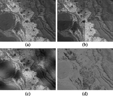
(a) The Martian rock image is again used as the base image. (b) Intensities in the four quadrants of the base image are changed by −30, −10, 10, and 30. (c) Assuming the base image contains n _r rows and n _c columns, intensity I at pixel (x,y) in the base image is replaced with O=I+50sin(4πy/n _r)cos(4πx/n _c). (d) Intensity I in the base image is replaced with O=I(1+cos(πI/255)). These images are of size 400×300 pixels. Image (a) when paired with images (b)–(d) constitute Sets 4–6
Full size image
2.
Intensities in the base image were changed based on their locations using a sinusoidal function. Assuming the base image has n _r rows and n _c columns, and the intensity at (x,y) is I, intensity I was replaced with O=I+50sin(4πy/n _r)cos(4πx/n _c) to obtain Fig. 2.27c. This simulates smoothly varying radiometric changes in a scene between times images 2.27a and 2.27c were captured.
3.
Intensities in the base image were changed by a sinusoidal function based on their values. Assuming I is the intensity at a pixel in the base image, intensity at the same pixel in the output was calculated from O=I(1+cos(πI/255)) to obtain the image shown in Fig. 2.27d. This image together with the base image can be considered images in different modalities.

Images in Figs. 2.27a and 2.27b are used as Set 4, images in Figs. 2.27a and 2.27c are used as Set 5, and images in Figs. 2.27a and 2.27d are used as Set 6. These images are used to determine the sensitivity of various measures to intensity differences between images.

To further evaluate the accuracy of the measures in matching multimodality images, bands 2 and 4 of the Landsat thematic mapper (TM) image shown in Figs. 2.28a and 2.28b were used. To test the measures against changes in camera exposure, the images in Figs. 2.29a and 2.29b, which were obtained at different exposures of a static scene by a stationary camera, are used.

The Landsat TM bands 2 and 4 in Fig. 2.28 are used as Set 7 and the multi-exposure images in Fig. 2.29 are used as Set 8 to further evaluate the sensitivity of the measures to intensity differences between images.

To determine the sensitivity of the measures to image blurring caused by camera defocus or change in image resolution, the Martian rock image shown again in Fig. 2.30a was smoothed with a Gaussian of standard deviation 1 pixel to obtain the image shown in Fig. 2.30b. The images in Figs. 2.30a and 2.30b are used as Set 9 to determine the sensitivity of the measures to image blurring.

To determine the sensitivity of the measures to occlusion and local geometric differences between images, stereo images of a Mars scene, courtesy of NASA, and aerial stereo images of the Pentagon, courtesy of CMU Robotics Institute, were used. These images are shown in Fig. 2.31. The Mars images represent Set 10 and the Pentagon images represent Set 11.

2.3.2 Evaluation Strategy

To measure and compare the performances of various similarity and dissimilarity measures, a number of template-matching scenarios were considered. Given two images, a template centered at each pixel (x,y) in the first image was taken and compared with windows of the same size in the neighborhood of (x,y) in the second image. Knowing true corresponding points in images in Sets 1–9, the percentage of correctly determined correspondences by each measure were determined.

As templates, square subimages of side 31 pixels were considered at each pixel in the first image in each set. Each such template was then searched for in the second image in the same set. Assuming a selected template was centered at pixel (x,y) in the first image, the search was performed in a square neighborhood of side 11 pixels centered at (x,y) in the second image. For stereo images, the search was performed only horizontally along corresponding scanlines in the images. In the Mars image set, the search area size was 81 pixels, and in the Pentagon data set, the search area size was 21 pixels centered at column x in scanline y in the second image. The search areas in the stereo images were selected in this manner in order to include the correct match within the search neighborhood.

Since the objective is to find the correspondence between centers of square regions in two images, when possible, intensities are weighted based on their distances to the centers of the matching template and window to allow intensities closer to the center of focus to influence the outcome more than intensities farther away. Gaussian weights of standard deviation equal to half the side of a template was used. For the Pearson correlation coefficient, Tanimoto measure, L ₁ norm, square L ₂ norm, and normalized square L ₂ norm, intensities in a template and the pairing window were multiplied by Gaussian weights to reduce the effect of pixels away from the centers of the template and window on a calculated measure. Gaussian weights were not used in measures that used the ratios or ranks of the intensities.

In measures that are formulated in terms of the JPD or the joint histogram of two images, instead of incrementing entry (i,j) in the joint histogram of two images by 1, if corresponding pixels in a pairing template and window had intensities i and j, entry (i,j) in the joint histogram was incremented by the Gaussian weight at the pixel location in template with intensity i or in window with intensity j. Incrementing the joint histogram entries in this manner counts pixels away from template and window center by a smaller amount than pixels closer to the template and window centers when creating the joint histogram. In this way, the JPD produces measures that are less sensitive to local geometric differences between images and, thus, improves matching of images with geometric differences, such as stereo images.

Since correspondence between pixels in images in Sets 1–9 are known, it is possible to tell the correctness of a template-matching outcome. The number of correct matches over the total number of matches attempted multiplied by 100 is used as the percent correct matches.

For image sets with unknown correspondences, such as the stereo images in Sets 10 and 11, the root-mean-squared intensity differences (RMSID) between corresponding pixels are used as the matching error. The smaller the RMSID is, the smaller the matching error and so the more accurate the correspondences will be.

2.4 Characteristics of Similarity/Dissimilarity Measures

Percent correct matches (true positives) for images in Sets 1–9 by the 16 similarity measures and the 11 dissimilarity measures are summarized in Tables 2.1 and 2.2. The value at an entry, for example, Pearson correlation and Set 1, was obtained by selecting square templates of side 31 pixels centered at pixels in the first image and searching for them in square search areas of side 11 pixels in the second image, and finding the percent matches that were correct. Since images in Set 1 are of size 400×300 pixels, (400−30−5)×(300−30−5) or 96725 possible templates of side 31 pixels are selected in the first image and searched for in the second image. Templates selected in this manner in the first image appear in their entirety in the second images. The number of correct matches over 96725 was multiplied by 100 to obtain the percent correct matches. This number was then entered at the entry for Pearson correlation and Set 1.

Table 2.1 Percent correct matches (true positives) of different similarity (top) and dissimilarity (bottom) measures using noisy image Sets 1–3, and intensity transformed image Sets 4 and 5. Newly introduced measures are shown in bold. Template size in each experiment was 31×31 pixels and search area size was 11×11 pixels. The three measures producing the most number of correct matches in each set are shown in bold, unless more than three measures produce 100% correct matches

Full size table

Table 2.2 Same as Table 2.1 except for using intensity transformed image Set 6, different band image Set 7, different exposure image Set 8, different resolution image Set 9, and stereo image Sets 10, and 11. For the stereo images in Sets 10 and 11 the average RMSIDs of corresponding pixels are shown. The smaller the average RMSID, the more accurate the correspondences are expected to be. For stereo images, the search was carried out in 1-D horizontally. For Set 10, the search area was 81 pixels, while for Set 11, the search area was 21 pixels. The three measures producing the least RMSID under stereo data sets are shown in bold

Full size table

Because the correct correspondences are not known for the images in Sets 10 and 11, the RMSID between corresponding pixels obtained by various measures were used to characterize matching accuracy. Average RMSID for all correspondences in a set was then used as the average RMSID for that set. For example, the entry for Pearson correlation and Set 11 was computed as follows. Since images in Set 11 are of size 512×512, using square templates of side 31 pixels and search areas of width 21 pixels, (512−30)×(512−30−10) or 227504 templates can be selected in the first image and searched in the second image. The RMSID for each match was found and the average of the 227504 RMSIDs was calculated and entered into the entry for Pearson correlation and Set 11.

If three or fewer measures produce 100% correct matches under an image set, the accuracies of the best three measures are shown in bold. For the stereo images (Sets 10 and 11), the three measures with the lowest average RMSID are shown in bold.

2.4.1 Sensitivity to Noise

Results in Table 2.1 show that under zero-mean noise, Kendall’s Tau and square L ₂ norm tie for the most number of correct matches, followed by Spearman’s Rho. Under zero-mean noise, measures that use intensity ranks generally perform well, while measures that are based on the JPD of image intensities perform poorly. Among the measures that are based on JPD, I _α-information appears least sensitive to noise, followed by material similarity and Tsallis mutual information.

2.4.2 Sensitivity to Scene Lighting/Camera Exposure

Sets 4 and 5 contain images simulating differences in scene lighting. Set 4 shows changes in scene lighting by fixed amounts at the four image quadrants and sharp changes across the boundary between the quadrants, while Set 5 shows changes that vary smoothly across the image domain. Measures that are formulated in terms of JPD perform well on Set 4 although ordinal measures perform equally well. For Set 5, the best measures are Pearson correlation, Tanimoto measure, Spearman’s Rho, Kendall’s Tau, normalized square L ₂ norm, and incremental sign distance.

Set 8 contains images obtained at different exposures of a camera. Changing the exposure has the same effect as changing scene lighting. Although no measure was able to produce 100% correct matches for this image set, many measures performed quite well, with the best measure being correlation ratio, followed by Pearson correlation and material similarity.

2.4.3 Sensitivity to Image Modality

Images in Sets 6 and 7 represent simulated and real multimodality images with intensities of corresponding pixels related by nonlinear mapping functions. Measures that are based on JPD work best on these image sets, as expected. The surprising result is from the incremental sign distance, which also performs quite well on Set 7, although it does not perform that well on Set 6. The best measure for Set 7 is the material similarity, the only measure producing 100% correct matches.

2.4.4 Sensitivity to Image Blurring

Set 9 contains images with blurring differences. This represents images at different resolutions. Measures that are computed from JPD generally perform poorly, while ordinal measures generally perform well. Among the ordinal measures, Kendall’s Tau and rank distance tie for the most number of correct matches. Other methods that produce 100% correct matches are Pearson correlation, Tanimoto measure, minimum ratio, L ₁ norm, square L ₂ norm, normalized square L ₂ norm, and intensity-ratio variance.

2.4.5 Sensitivity to Imaging View

Images from different views of a 3-D scene contain local geometric differences. Stereo images have this characteristic. Tests on the stereo images in Sets 10 and 11 reveal that traditionally used measures such as Pearson correlation and L ₁ norm perform well, while measures that are based on JPD perform the worst. Surprisingly, ordinal measures do not perform that well when applied to images with local geometric differences. The best measure for Set 10 was normalized square L ₂ norm followed by Tanimoto measure and Pearson correlation. The best measure for Set 11 was minimum ratio followed by L ₁ Norm and Tanimoto measure. Examining results in Table 2.2 we see Pearson correlation, Tanimoto measure, minimum ratio, L ₁ norm, square L ₂ norm, and normalized square L ₂ norm all have very close performance measures with the remaining measures producing much worse results.

To visually evaluate the quality of stereo correspondences obtained by these measures, after finding the correspondences, the right image in a stereo pair was resampled to align with the left image. The overlaid images are shown in Figs. 2.32 and 2.33. Image (a) in each case shows overlaying of the original stereo images. Figs. 2.32b–d show resampling of the right image to the space of the left image using the correspondences obtained by normalized square L ₂ norm, Tanimoto measure, and Pearson correlation, respectively. The left image in a stereo pair is shown in red, while the right image is shown in green. Yellow pixels show overlaid pixels with very close intensities, most likely representing correct correspondences, and red and green pixels show overlaid pixels with quite different intensities. These pixels most likely represent incorrect correspondences. The red boundary region in each overlaid image shows pixels where matching was not performed because parts of templates centered at those pixels fall outside the image during matching.

The matching results in Fig. 2.33 show correspondences obtained by minimum ratio, L ₁ norm, and Tanimoto measure. Most mismatches seem to be occurring at points visible to only one of the cameras due to occlusion, or in homogeneous regions, where there is lack of sufficient detail for accurate matching.

It is interesting to note that the median of absolute differences and the median of square differences have not performed as well as L ₁ norm and square L ₂ norm. Due to very small occlusions in these stereo images, by discarding half of the pixels that produce the highest 50% differences, not only the occluded pixels are discarded, pixels that are critical in distinguishing adjacent neighborhoods from each other are discarded, dulling the matching process.

2.4.6 Dependency on Template Size

As template size is increased, more image information is used in template matching, increasing the correspondence accuracy. This is only true when the images do not have geometric differences. When the images have geometric differences and the images are overlaid at a point of interest, points farther away from the point of interest will displace more, confusing the matching process. When dealing with stereo images, matching accuracy increases as template size is increases up to a point, beyond which increasing template size decreases matching accuracy.

Increasing template size from 31 to 51 pixels in Sets 1–9, and decreasing the template size from 31 to 21 pixels for Sets 10 and 11, the results shown in Tables 2.3 and 2.4 are obtained. Increasing template size clearly improves matching accuracy for Sets 1–9. Improvement is observed the most among measures that are formulated in terms of JPD. In particular, the accuracies of I _α-information and exclusive f-information improve considerably, even under high noise level. The accuracy of ordinal measures also increases considerably, especially that for Spearman’s Rho, which produces perfect matches for all 9 image sets and surpasses the performances of Kendall’s Tau and correlation ratio. Least affected by change in template size are minimum ratio, correlation ratio, incremental sign distance, and rank distance. Since these measures already perform quite well with small templates, if small templates are required, they are the measures to use.

Table 2.3 Similar to Table 2.1 except for using square templates of side 51 pixels

Full size table

Table 2.4 Similar to Table 2.2 except for using square templates of side 51 pixels in Sets 6–9 and square templates of side 21 pixels in Sets 10 and 11

Full size table

2.4.7 Speed

In addition to accuracy, speed determines the performance of a similarity or dissimilarity measure. Computation time in milliseconds needed by a Windows PC with a 3.2 GHz processor to find a pair of corresponding points in the images for each case in Tables 2.1–2.4 is determined and shown in Tables 2.5–2.8, respectively.

Table 2.5 Computation time in milliseconds needed to find a pair of corresponding points in Table 2.1 on a Windows PC with a 3.2 GHz processor

Full size table

From the contents of Tables 2.5–2.8, we can conclude that ordinal measures are the most expensive measures followed by measures that are based on the JPD of image intensities. The three fastest methods are square L ₂ norm, L ₁ norm, and intensity-ratio variance. The fact that square L ₂ norm is widely used in stereo matching is no surprise as it has the fastest speed among the measures tested with accuracy that is very close to the best accuracy achievable.

Changing template size changes the computation time. Computation time varies from a linear function of template size n to a quadratic function of n. Computation time when using templates of side 51 pixels in Sets 1–9 and templates of side 21 pixels in Sets 10 and 11 are shown in Tables 2.7 and 2.8. When compared with Tables 2.5 and 2.6, we see that again square L ₂ norm is the fastest and the gap between slower and faster measures widens for Sets 1–9. For Sets 10 and 11, the gap in computation time between slow and fast measures narrows as template size is decreased.

Table 2.6 Computation time in milliseconds needed to find a pair of corresponding points in Table 2.2 on a Windows PC with a 3.2 GHz processor

Full size table

Table 2.7 Computation time in milliseconds needed to find a pair of corresponding points in Table 2.3 on a Windows PC with a 3.2 GHz processor

Full size table

Table 2.8 Computation time in milliseconds needed to find a pair of corresponding points in Table 2.4 on a Windows PC with a 3.2 GHz processor

Full size table

The smallest increase in computation time as template size is increased is observed in measures that use JPD. This is because a portion of the computation time is spent by these measures to create the JPD, which is a linear function of template size n, and a portion of the computation time that is independent of n is spent on calculating a similarity or dissimilarity measure from the obtained JPD. Increase in template size, therefore, only linearly increases the time for creating the JPD, which is a small portion of the overall computation time. Measures that have computational complexities a linear function of n, such as correlation coefficient, Tanimoto measure, minimum ratio, L ₁ norm, square L ₂ norm, and intensity ratio variance also have the smallest increase in computation time with an increase in n.

The largest increase in computation time as a function of n is observed by measures that use ranks of intensities, especially those that are quadratic functions of n, such as greatest deviation, Kendall’s Tau, and the ordinal measure.

2.5 Choosing a Similarity/Dissimilarity Measure

Each similarity/dissimilarity measure has its strengths and weaknesses. A measure that performs well on one type of images may perform poorly on another type of images. Therefore, an absolute conclusion cannot be reached about the superiority of one measure against another. However, the experimental results obtained on various image types and various image differences reveal that Pearson correlation coefficient, Tanimoto measure, minimum ratio, L ₁ norm, square L ₂ norm, and intensity ratio variance overall perform better than other measures. If the images are captured under different exposures of a camera or under different lighting of a scene, the results show that Pearson correlation coefficient, Tanimoto measure, normalized square L ₂ norm, and incremental sign distance perform better than others.

Different-modality images are most efficiently and accurately matched by intensity-mapping-ratio variance, joint entropy, energy of JPD, correlation ratio, and Spearman’s Rho. Although in the past, measures solely based on JPD have been used to match images in different modalities, experimental results obtained in this chapter show that ordinal measures such as correlation ratio and Spearman’s Rho are equally effective and more efficient than many of the JPD measures in the matching of multimodality images.

Stereo images are most efficiently and accurately matched using Pearson correlation, Tanimoto measure, minimum ratio, L ₁ norm, square L ₂ norm, and normalized square L ₂ norm. It is clear that when the images being matched are stereo, the measures to avoid are those that are based on JPD as not only are they computationally very expensive, they are the least accurate. Outliers and noise quickly degrade such measures. Some of the ordinal measures such as Spearman’s Rho, Kendall’s Tau, and rank distance produce accuracies that are close to those obtained by Pearson correlation, Tanimoto measure, minimum ratio, L ₁ norm, square L ₂ norm, and normalized square L ₂ norm, but they are not as efficient and so are not recommended in stereo matching.

Considering the accuracies of the measures obtained using the images in Sets 1–9, we find that correlation ratio followed by intensity-mapping-ratio variance produce the best accuracy when template size is relatively small (side 31 pixels). At a larger template size (side 51 pixels), Spearman’s Rho takes the lead followed by correlation ratio. Therefore, if a single measure is to be used to compare images containing noise and intensity differences but no geometric differences, correlation ratio, Spearman’s rho, and Kendall’s Tau are the ones to choose. Considering computational efficiency as well as accuracy, correlation ratio is clearly the choice followed by Spearman’s Rho.

If a single measure is to be used to match all 11 image sets, we see that Pearson correlation and Tanimoto measure receive the highest score as they manage to match 7 out of 11 image sets either perfectly or better than all other measures. This is followed by Kendall’s Tau and correlation ratio. At a larger template size, Spearman’s Rho takes the lead, either perfectly matching 9 out of 11 images sets or matching them better than any other measure. This is followed by normalized square L ₂, which manages to match 8 out of 11 sets either perfectly or better than other measures.

Among the four newly introduced measures, minimum ratio was found the best in matching the stereo images in Set 11 when using small templates and the best in matching the stereo images in Sets 10 and 11 when using moderate size templates. Also, because of its very low computational cost it is the similarity measure of choice when matching stereo images. Energy of JPD when compared to Shannon mutual information produces a better accuracy on 10 out of the 11 image sets for small templates and 8 out of the 11 image sets for moderate size templates. Considering that it requires nearly half the computation time of Shannon mutual information, it can replace Shannon mutual information to increase both speed and accuracy. Material similarity produced the highest accuracy in matching multimodality images in Sets 7 and 8 when using a relatively small template size and produced perfect matches for the same image sets at a larger template size, thus making it the most accurate measure in matching multimodality images. Material similarity is, however, computationally more expensive than Shannon mutual information. Rank distance is an ordinal measure that has the fastest speed among the ordinal measures and has an accuracy that falls somewhere in the middle among the ordinal measures tested.

2.6 Preprocessing Considerations

Similarity and dissimilarity measures that are based on JDP or intensity ranks are not sensitive to sensor characteristics or scene lighting but are computationally very expensive. On the other hand, measures that use raw image intensities are fast but are sensitive to differences in sensor characteristics and scene lighting. In order to take advantage of the fast speed of the latter and the robustness of the former, the images may be preprocessed, normalizing the intensities before using them in the calculation of a measure.

If the images are known to contain noise, one may filter out the noise before attempting to compute the similarity/dissimilarity between them. If the images are known to contain impulse noise, median filtering may be used to reduce or remove noise, and if the images are known to contain zero-mean noise, Gaussian filtering may be used to reduce the effect of noise. Since image filtering changes intensities even at pixels that are not affected by noise, the filter kernel should be sufficiently small to avoid smoothing the image structures but large enough to reduce sufficient noise to produce an accurate similarity/dissimilarity measure.

To preserve image structures while reducing noise, filter kernels that change in shape and size are most desirable [2, 34, 59, 67]. Figure 2.34 compares adaptive smoothing versus traditional smoothing at the presence of zero-mean noise.

If the images are obtained under different lighting conditions, through a preprocessing operation image intensities can be normalized to remove global intensity differences between them. In the monotonicity operation proposed by Kories and Zimmerman [44], a 3×3 window is considered at a pixel, and the intensity at the pixel is replaced by a number between 0 and 8 depending on the number of intensities within the 3×3 window that are smaller than the intensity at the pixel. Intensities are newly assigned that depend on their relative values within a small neighborhood rather than their absolute values globally. This process will reduce or remove global intensity differences between images.

The rank transform proposed by Zabih and Woodfill [111], replaces the local intensity distribution of an image with values in the range 0 to d ²−1 similar to monotonicity operation, where d=2r+1 is an odd number showing the side of the square window centered at the pixel under consideration. This mapping is particularly effective when high-dynamic range images are used. The method brightens areas that are too dark and darkens areas that are too bright.

Suppose the center pixel in a d×d neighborhood is denoted by p and the intensity at p is I(p). Also, suppose the intensity at pixel p′ (p′≠p) in that neighborhood is I(p′). If the number of pixels within the neighborhood where I(p′)<I(p) is m, then m is considered the rank of p and assigned to p. This is the same as monotonicity operation except for using a neighborhood larger than 3×3.

If a 16×16 neighborhood is selected, the center pixel can be considered the 128th pixel within the neighborhood when counted in raster scan order. Then, the rank of the intensity at the center pixel will have a value between 0 and 255 depending on whether from none to all intensities within the neighborhood are smaller than the intensity at the center pixel. Mapping intensities in this manner enables removing global intensity differences between images. An example of intensity mapping using 17×17 neighborhoods is given in Fig. 2.35. Ranks greater than 255, which rarely occur, are set to 255. Figures 2.35a and 2.35b after rank transform are shown in Figs. 2.35c and 2.35d, respectively. The images after rank transform are indistinguishable.

At the presence of outliers (occlusions), rank transform has been found to improve matching accuracy [111]. This can be attributed to the fact that at occluded boundaries there are sharp intensity changes and rank transform dulls the sharp changes, reducing the occlusion effect and producing more accurate matches. However, this dulling effect can worsen matching accuracy when applied to images that do not contain occlusions. Rank transform intensity mapping when applied to high-contrast and noise-free images may reduce image information sufficiently to worsen matching accuracy. Therefore, care should be taken when choosing a preprocessing operation in image matching.

References

Alliney, S., Morandi, C.: Digital image registration using projections. IEEE Trans. Pattern Anal. Mach. Intell. 8(2), 222–233 (1986)
Article Google Scholar
Alvarez, L., Lions, P.-L., Morel, J.-M.: Image selective smoothing and edge detection by nonlinear diffusion II. SIAM J. Numer. Anal. 29(3), 845–866 (1992)
Article MathSciNet MATH Google Scholar
Anuta, P.E.: Spatial registration of multispectral and multitemporal digital imagery using fast Fourier transform techniques. IEEE Trans. Geosci. Electron. 8(4), 353–368 (1970)
Article Google Scholar
Ayinde, O., Yang, Y.-H.: Face recognition approach based on rank correlation of gabor-filtered images. Pattern Recognit. 35, 1275–1289 (2002)
Article MATH Google Scholar
Barnea, D.I., Silverman, H.F.: A class of algorithms for fast digital image registration. IEEE Trans. Comput. 21(2), 179–186 (1972)
Article MATH Google Scholar
Bhat, N., Nayar, S.K.: Ordinal measures for image correspondence. IEEE Trans. Pattern Anal. Mach. Intell. 20(4), 415–423 (1998)
Article Google Scholar
Blakeman, J.: On tests for linearity of regression in frequency distributions. Biometrika 4(3), 332–350 (1905)
Article Google Scholar
Borland, L., Plastino, A.R., Tsallis, C.: Information gain within nonextensive thermostatistics. J. Math. Phys. 39(12), 6490–6501 (1998)
Article MathSciNet MATH Google Scholar
Chambon, S., Crouzil, A.: Dense matching using correlation: new measures that are robust near occlusions. In: Proc. British Machine Vision Conference, vol. 1, pp. 143–152 (2003)
Google Scholar
Chambon, S., Crouzil, A.: Similarity measures for image matching despite occlusions in stereo vision. Pattern Recognit. 44, 2063–2075 (2011)
Article Google Scholar
Chen, Y.-P.: A note on the relationship between Spearman’s ρ and Kendall’s τ for extreme order statistics. J. Stat. Plan. Inference 137, 2165–2171 (2007)
Article MATH Google Scholar
Chen, Q.-S.: Matched filtering techniques. In: Le Moigne, J., Netanyahu, N.S., Eastman, R.D. (eds.) Image Registration for Remote Sensing, pp. 112–130. Cambridge University Press, Cambridge (2011)
Chapter Google Scholar
Chen, H.-M., Varshney, P.K., Arora, M.K.: Performance of mutual information similarity measure for registration of multitemporal remote sensing images. IEEE Trans. Geosci. Remote Sens. 41(11), 2445–2454 (2003)
Article Google Scholar
Cole-Rhodes, A.A., Johnson, K.L., LeMoigne, J., Zavorin, I.: Multiresolution registration of remote sensing imagery by optimization of mutual information using a stochastic gradient. IEEE Trans. Image Process. 12(12), 1495–1511 (2003)
Article MathSciNet Google Scholar
Collignon, A., Maes, F., Delaere, D., Vandermeulen, D., Suetens, P., Marchal, A.: Automated multi-modality image registration based on information theory. In: Proc. Information Processing in Medicine Conf., pp. 263–274 (1995)
Google Scholar
Conners, R.W., Harlow, C.A.: A theoretical comparison of texture algorithms. IEEE Trans. Pattern Anal. Mach. Intell. 2(3), 204–222 (1980)
Article MATH Google Scholar
Coselmon, M.M., Balter, J.M., McShan, D.L., Kessler, Marc L.: Mutual information based CT registration of the lung at exhale and inhale breathing states using thin-plate splines. Med. Phys. 31(11), 2942–2948 (2004)
Article Google Scholar
Crathorne, A.R.: Calculation of the correlation ratio. J. Am. Stat. Assoc. 18(139), 394–396 (1922)
Article Google Scholar
Cvejic, N., Canagarajah, C.N., Bull, D.R.: Information fusion metric based on mutual information and Tsallis entropy. Electron. Lett. 42(11), 626–627 (2006)
Article Google Scholar
D’Agostino, E., Maes, F., Vandermeulen, D., Suetens, P.: A viscous fluid model for multimodal non-rigid image registration using mutual information. Med. Image Anal. 7, 565–575 (2003)
Article Google Scholar
De Castro, E., Morandi, C.: Registration of translated and rotated images using finite Fourier transforms. IEEE Trans. Pattern Anal. Mach. Intell. 9(5), 700–703 (1987)
Article Google Scholar
dos Santos, R.J.V.: Generalization of Shannon’s theorem of Tsallis entropy. J. Math. Phys. 38(8), 4104–4107 (1997)
Article MathSciNet MATH Google Scholar
Duda, R.O., Hart, P.E., Stork, D.G.: Pattern Classification, 2nd edn., p. 187. Wiley-Interscience, New York (2001)
MATH Google Scholar
Duncan, T.E.: On the calculation of mutual information. SIAM Journal. Appl. Math. 19(1), 215–220 (1970)
MATH Google Scholar
Evangelidis, G.D., Psarakis, E.Z.: Parametric image alignment using enhanced correlation coefficient maximization. IEEE Trans. Pattern Anal. Mach. Intell. 30(10), 1858–1865 (2008)
Article Google Scholar
Fitch, A.J., Kadyrov, A., Christmas, W.J., Kittler, J.: Orientation correlation. In: British Machine Vision Conf., vol. 1, pp. 133–142 (2002)
Google Scholar
Fredricks, G.A., Nelsen, R.B.: On the relationship between Spearman’s rho and Kendall’s tau for pairs of continuous random variables. J. Stat. Plan. Inference 137, 2143–2150 (2007)
Article MathSciNet MATH Google Scholar
Gao, Z., Gu, B., Lin, J.: Monomodal image registration using mutual information based methods. Image Vis. Comput. 26, 164–173 (2008)
Article Google Scholar
Gauthier, T.D.: Detecting trends using Spearman’s rank correlation, coefficient. Environ. Forensics 2, 359–362 (2001)
Article Google Scholar
Gel’fand, I.M., Yaglom, A.M.: Calculation of the amount of information about a random function contained in another such function. Am. Math. Soc. Trans. 2(12), 199–246 (1959)
MathSciNet Google Scholar
Gibbons, J.D.: Nonparametric Methods for Quantitative Analysis, 2nd edn., p. 298. American Science Press, Columbus (1985)
MATH Google Scholar
Gideon, R.A., Hollister, R.A.: A rank correlation coefficient. J. Am. Stat. Assoc. 82(398), 656–666 (1987)
Article MathSciNet MATH Google Scholar
Gilpin, A.R.: Table for conversion of Kendall’s tau and Spearman’s rho within the context of measures of magnitude of effect for meta-analysis. Educ. Psychol. Meas. 53, 87–92 (1993)
Article Google Scholar
Goshtasby, A., Satter, M.: An adaptive window mechanism for image smoothing. Comput. Vis. Image Underst. 111, 155–169 (2008)
Article Google Scholar
Goshtasby, A., Gage, S., Bartholic, J.: A two-stage cross-correlation approach to template matching. IEEE Trans. Pattern Anal. Mach. Intell. 6(3), 374–378 (1984)
Article Google Scholar
Harter, H.L.: Nonuniqueness of least absolute values regression. Commun. Stat. Theor. Math. A6(9), 829–838 (1977)
Article MATH Google Scholar
Hill, D.L.G., Hawkes, D.J., Harrison, N.A., Ruff, C.F.: A strategy for automated multimodality image registration incorporating anatomical knowledge and image characteristics. In: Proc. 13th Int’l Conf. Information Processing in Medical Imaging, pp. 182–196 (1993)
Chapter Google Scholar
Huntington, E.V.: Mathematics and statistics, with an elementary account of the correlation coefficient and the correlation ratio. Am. Math. Mon. 26(10), 421–435 (1919)
Article MathSciNet MATH Google Scholar
Jizba, P., Arimitsu, T.: Observability of Rényi entropy. Phys. Rev. E 69, 026128 (2004), pp. 1–12
Article MathSciNet Google Scholar
Kaneko, S., Murase, I., Igarashi, S.: Robust image registration by increment sign correlation. Pattern Recognit. 35(10), 2223–2234 (2002)
Article MATH Google Scholar
Kendall, M.G.: A new measure of rank correlation. Biometrika 30, 81–93 (1938)
MathSciNet MATH Google Scholar
Kendall, M.G.: Rank Correlation Methods, 3rd edn., p. 12. Charles Birchall and Sons, Liverpool (1962)
Google Scholar
Klein, S., Staring, M., Pluim, J.P.W.: Evaluation of optimization methods for nonrigid medical image registration using mutual information and B-splines. IEEE Trans. Image Process. 16(12), 2879–2890 (2007)
Article MathSciNet Google Scholar
Kories, R., Zimmerman, G.: A versatile method for the estimation of displacement vector fields from image sequences. In: Workshop on Motion Representation and Analysis, pp. 101–107 (1986)
Google Scholar
Kotlyar, M., Fuhrman, S., Ableson, A., Somogyi, R.: Spearman correlation identifies statistically significant gene expression clusters in spinal cord development and injury. Neurochem. Res. 27(10), 1133–1140 (2002)
Article Google Scholar
Krotosky, S.J., Trivedi, M.M.: Mutual information based registration of multimodal stereo video for person tracking. Comput. Vis. Image Underst. 106, 270–287 (2007)
Article Google Scholar
Kruskal, W.: Ordinal measures of association. J. Am. Stat. Assoc. 53, 814–861 (1958)
Article MathSciNet MATH Google Scholar
Kuglin, C.D., Hines, D.C.: The phase correlation image alignment method. In: Proc. Int’l Conf. Cybernetics and Society, pp. 163–165 (1975)
Google Scholar
Lan, Z.-D., Mohr, R.: Robust matching by partial correlation. In: Proc. 6th British Machine Vision Conf., pp. 651–660 (1995)
Google Scholar
Lau, Y.H., Braun, M., Hutton, B.F.: Non-rigid image registration using a median-filtered coarse-to-fine displacement field and a symmetric correlation ratio. Phys. Med. Biol. 46, 1297–1319 (2001)
Article Google Scholar
Likar, B., Pernuš, F.: A hierarchical approach to elastic registration based on mutual information. Image Vis. Comput. 19, 33–44 (2001)
Article Google Scholar
Liu, L., Jiang, T., Yang, J., Zhu, C.: Fingerprint registration by maximization of mutual information. IEEE Trans. Image Process. 15(5), 1100–1110 (2006)
Article Google Scholar
Maes, F., Collignon, A., Vandermeulen, D., Marchal, G., Suetens, P.: Multimodality image registration by maximization of mutual information. IEEE Trans. Med. Imaging 16(2), 187–198 (1997)
Article Google Scholar
Maes, F., Vandermeulen, D., Suetens, P.: Comparative evaluation of multiresolution optimization strategies for multimodality image registration by maximization of mutual information. Med. Image Anal. 3(4), 373–386 (1999)
Article Google Scholar
Maes, F., Vandermeulen, D., Suetens, P.: Medical image registration using mutual information. Proc. IEEE 91(10), 1699–1722 (2003)
Article Google Scholar
Martin, S., Morison, G., Nailon, W., Durrani, T.: Fast and accurate image registration using Tsallis entropy and simultaneous perturbation stochastic approximation. Electron. Lett. 40(10), 595–597 (2004)
Article Google Scholar
Matthäus, L., Trillenberg, P., Fadini, T., Finke, M., Schweikard, A.: Brain mapping with transcranial magnetic stimulation using a refined correlation ratio and Kendall’s τ. Stat. Med. 27, 5252–5270 (2008)
Article MathSciNet Google Scholar
McLaughlin, P.W., Narayana, V., Kessler, M., McShan, D., Troyer, S., Marsh, L., Hixson, G., Roberson, P.L.: The use of mutual information in registration of CT and MRI datasets post permanent implant. Brachytherapy 3, 61–70 (2004)
Article Google Scholar
Meer, P., Park, R.H., Cho, K.: Multiresolution adaptive image smoothing. CVGIP, Graph. Models Image Process. 56(2), 140–148 (1994)
Article Google Scholar
Mellor, M., Brady, M.: Phase mutual information as a similarity measure for registration. Med. Image Anal. 9, 330–343 (2005)
Article Google Scholar
Milko, S., Melvaer, E.L., Samset, E., Kadir, T.: Evaluation of the bivariate correlation ratio similarity measure metric for rigid registration of US/MR images of the liver. Int. J. Comput. Assisted Radiol. Surg. 4, 147–155 (2009)
Article Google Scholar
Muselet, D., Trémeau, A.: Rank correlation as illumination invariant descriptor for color object recognition. In: Proc. 15th Int’l Conf. Image Processing, pp. 157–160 (2008)
Google Scholar
Nalpantidis, L., Sirakoulis, G.Ch., Gasteratos, A.: A dense stereo correspondence algorithm for hardware implementation with enhanced disparity selection. In: Lecture Notes in Computer Science, vol. 5138, pp. 365–370. Springer, Berlin (2008)
Google Scholar
Okutomi, M., Kanade, T.: A locally adaptive window for signal matching. Int. J. Comput. Vis. 7(2), 143–162 (1992)
Article Google Scholar
Pearson, K.: Contributions to the mathematical theory of evolution, III, Regression, heredity, and panmixia. Philos. Trans. R. Soc. Lond. Ser. A 187, 253–318 (1896)
Article MATH Google Scholar
Pearson, K.: Mathematical contributions to the theory of evolution, XIV, on the general theory of skew correlation and non-linear regression. In: Drapers’ Company Research Memoirs, Biometric Series, II. Dulau and Co., London (1905), 54 p.
Google Scholar
Perona, P., Malik, J.: Scale-space and edge detection using anisotropic diffusion. IEEE Trans. Pattern Anal. Mach. Intell. 12(7), 629–639 (1990)
Article Google Scholar
Pluim, J.P.W., Antoine, J.B., Viergever, M.: Image registration by maximization of combined mutual information and gradient information. IEEE Trans. Med. Imaging 19(8), 809–814 (2000)
Article Google Scholar
Pluim, J.P.W., Maintz, J.B.A., Viergever, M.A.: f-information measures in medical image registration. IEEE Trans. Med. Imaging 23(12), 1506–1518 (2004)
Article Google Scholar
Raggio, G.A.: Properties of q-entropies. J. Math. Phys. 36(9), 4785–4791 (1995)
Article MathSciNet MATH Google Scholar
Rangarajan, A., Chui, H., Duncan, J.: Rigid point feature registration using mutual information. Med. Image Anal. 3(4), 425–440 (1999)
Article Google Scholar
Reddy, B.S., Chatterji, B.: An FFT-based technique for translation, rotation and scale invariant image registration. IEEE Trans. Image Process. 5(8), 1266–1271 (1996)
Article Google Scholar
Rényi, A.: On measures of entropy and information. In: Proc. Fourth Berkeley Symposium on Mathematical Statistics Probability, vol. 1, pp. 547–561. University of California Press, Berkeley (1961). Also available in Selected Papers of Alfréd Rényi 2, 525–580 (1976)
Google Scholar
Rényi, A.: Probability Theory. American Elsevier Publishing, North Holland, Amsterdam (1970)
Google Scholar
Roche, A., Malandain, G., Pennec, X., Ayache, N.: The correlation ratio as a new similarity measure for multimodal image registration. Lect. Notes Comput. Sci. 1496, 1115–1124 (1998). Also, see Multimodal Image Registration by Maximization of the Correlation Ratio, Report No. 3378, Institute de Research en Informatique et en Automatique, Aug. 1998
Article Google Scholar
Roche, A., Pennec, X., Malandain, G., Ayache, N.: Rigid registration of 3-D ultrasound with MR images: A new approach combining intensity and gradient information. IEEE Trans. Med. Imaging 20(10), 1038–1049 (2001)
Article Google Scholar
Rosenfeld, A., Vanderburg, G.J.: Coarse-fine template matching. IEEE Trans. Syst. Man Cybern. 7(2), 104–107 (1977)
Article Google Scholar
Rougon, N.F., Petitjean, C., Preteux, F.: Variational non-rigid image registration using exclusive f-information. In: Proc. Int’l Conf. Image Processing, Los Alamitos, CA, pp. 703–706 (2003)
Google Scholar
Rousseeuw, P.J.: Least median of squares regression. J. Am. Stat. Assoc. 79(388), 871–880 (1984)
Article MathSciNet MATH Google Scholar
Rousseeuw, P.J., Leroy, A.M.: Robust Regression and Outlier Detection. Wiley, New York (1987)
Book MATH Google Scholar
Rueckert, D., Clarkson, M.J., Hill, D.L., Hawkes, D.J.: Non-rigid registration using high-order mutual information. In: Proc. SPIE Image Processing: Medical Imaging, vol. 3979, pp. 438–447 (2000)
Google Scholar
Shannon, C.E.: The mathematical theory of communication. In: Shannon, C.E., Weaver, W. (eds.) The Mathematical Theory of Communication, pp. 29–125. University of Illinois Press, Urbana (1949), reprint 1998
Google Scholar
Shapiro, L.G., Stockman, G.C.: Computer Vision, p. 219. Prentice Hall, Upper Saddle River (2001)
Google Scholar
Shieh, G.S.: A weighted Kendall’s tau statistic. Stat. Probab. Lett. 39, 17–24 (1998)
Article MathSciNet MATH Google Scholar
Skouson, M.B., Guo, Q., Liang, Z.-P.: A bound on mutual information for image registration. IEEE Trans. Med. Imaging 20(8), 843–846 (2001)
Article Google Scholar
Spearman, C.: The proof and measurement of association between two things. Am. J. Psychol. 15(1), 72–101 (1904)
Article Google Scholar
Stone, H.S.: Fast correlation and phase correlation. In: Le Moigne, J., Netanyahu, N.S., Eastman, R.D. (eds.) Image Registration for Remote Sensing, pp. 79–111. Cambridge University Press, Cambridge (2011)
Chapter Google Scholar
Studholme, C., Hill, D.L.G., Hawkes, D.J.: Automated 3D registration of truncated MR and CT images of the head. In: Proc. British Machine Vision Conf., pp. 27–36 (1995)
Google Scholar
Studholme, C., Hill, D.L.G., Hawkes, D.J.: An overlap invariant entropy measure of 3D medical image alignment. Pattern Recognit. 32, 71–86 (1999)
Article Google Scholar
Tao, G., He, R., Datta, S., Narayana, P.A.: Symmetric inverse consistent nonlinear registration driven by mutual information. Comput. Methods Programs Biomed. 95, 105–115 (2009)
Article Google Scholar
Tedeschi, W., Müller, H.-P., de Araujo, D.B., Santos, A.C., Neves, U.P.C., Erné, S.N., Baffa, O.: Generalized mutual information fMRI analysis: A study of the Tsallis q parameter. Physica A 344, 705–711 (2004)
Article Google Scholar
Theodoridis, S., Koutroumbas, K.: Pattern Recognition, 4th edn. Academic Press, New York (2009), pp. 602, 605, 606
Google Scholar
Thévenaz, P., Unser, M.: Optimization of mutual information for multiresolution image registration. IEEE Trans. Image Process. 9(12), 2083–2099 (2000)
Article MATH Google Scholar
Tsallis, C.: Possible generalization of Boltzmann-Gibbs statistics. J. Stat. Phys. 52, 479–487 (1988)
Article MathSciNet MATH Google Scholar
Vajda, I.: Theory of Statistical Evidence and Information, p. 309. Kluwer Academic, Dordrecht (1989)
Google Scholar
van Hecke, W., Leemans, A., D’Angostino, E., De Backer, S., Vandervliet, E., Parizel, P.M., Sijbers, J.: Nonrigid coregistration of diffusion tensor images using a viscous fluid model and mutual information. IEEE Trans. Med. Imaging 26(11), 1598–1612 (2007)
Article Google Scholar
Vanderburg, G.J., Rosenfeld, A.: Two-stage template matching. IEEE Trans. Comput. 26, 384–393 (1977)
Article Google Scholar
Venot, A., Leclerc, V.: Automated correction of patient motion and gray values prior to subtraction in digitized angiography. IEEE Trans. Med. Imaging 3, 179–186 (1984)
Article Google Scholar
Venot, A., Lebruchec, J.F., Golmard, J.L., Roucayrol, J.C.: An automated method for the normalization of scintigraphic images. J. Nucl. Med. 24, 529–531 (1983)
Google Scholar
Venot, A., Devaux, J.Y., Herbin, M., Lebruchec, J.F., Dubertret, L., Raulo, Y., Roucayrol, J.C.: An automated system for the registration and comparison of photographic images in medicine. IEEE Trans. Med. Imaging 7(4), 298–303 (1988)
Article Google Scholar
Viola, P., Wells, W.M. III: Alignment by maximization of mutual information. Int. J. Comput. Vis. 24(2), 137–154 (1997)
Article Google Scholar
Wachowiak, M.P., Smolikova, R., Tourassi, G.D., Elmaghraby, A.S.: Similarity metrics based on nonadditive entropies for 2D-3D multimodal biomedical image registration. In: Medical Imaging Conf., Proc. SPIE, vol. 5032, San Diego, CA, pp. 1090–1100 (2003)
Google Scholar
Walimbe, V., Zagrodsky, V., Raja, S., Jaber, W.A., DiFilippo, F.P., Garcia, M.J., Brunken, R.C., Thomas, J.D., Shekhar, R.: Mutual information-based multimodality registration of cardiac ultrasound and SPECT images: a preliminary investigation. Int. J. Card. Imaging 19, 483–494 (2003)
Article Google Scholar
Wells, W.M. III, Viola, P., Atsumi, H., Nakajima, S., Kikinis, R.: Multi-modal volume registration by maximization of mutual information. Med. Image Anal. 1(1), 35–51 (1996)
Article Google Scholar
Wong, K.K., Yang, E.S., Wu, E.X., Tse, H.-F., Wong, S.T.: First-pass myocardial perfusion image registration by minimization of normalized mutual information. J. Magn. Reson. Imaging 27, 529–537 (2008)
Article Google Scholar
Woods, R.P., Cherry, S.R., Mazziotta, J.C.: Rapid automated algorithm for aligning and reslicing PET images. J. Comput. Assist. Tomogr. 16, 620–633 (1992)
Article Google Scholar
Woods, R.P., Mazziotta, J.C., Cherry, S.R.: MRI-PET registration with automated algorithm. J. Comput. Assist. Tomogr. 17(4), 536–546 (1993)
Article Google Scholar
Xu, P., Yao, D.: A study on medical image registration by mutual information with pyramid data structure. Comput. Biol. Med. 37, 320–327 (2007)
Article Google Scholar
Yokoi, T., Soma, T., Shinohara, H., Matsuda, H.: Accuracy and reproducibility of co-registration techniques based on mutual information and normalized mutual information for MRI and SPECT brain images. Ann. Nucl. Med. 18(8), 659–667 (2004)
Article Google Scholar
Yue, S., Pilon, P., Cavadias, G.: Power of the Mann-Kendall and Spearman’s rho tests for detecting monotonic trends in hydrological series. J. Hydrol. 259, 254–271 (2002)
Article Google Scholar
Zabih, R., Woodfill, J.: Non-parametric local transforms for computing visual correspondence. In: European Conf. Computer Vision, Stockholm, Sweden, pp. 151–158 (1994)
Google Scholar
Zhu, H., Shu, H., Xia, T., Luo, L., Coatrieux, J.L.: Translation and scale invariants of Tchebichef moments. Pattern Recognit. 40, 2530–2542 (2007)
Article MATH Google Scholar
Zyczkowski, K.: Rényi extrapolation of Shannon entropy. Open Syst. Inf. Dyn. 10, 297–310 (2003)
Article MathSciNet MATH Google Scholar

Download references

Author information

Authors and Affiliations

Dept. Computer Science and Engineering, 303 Russ Engineering Center, Wright State University, Dayton, OH, USA
Prof. A. Ardeshir Goshtasby

Authors

Prof. A. Ardeshir Goshtasby
View author publications
You can also search for this author in PubMed Google Scholar

Corresponding author

Correspondence to A. Ardeshir Goshtasby .

Rights and permissions

Reprints and permissions

Copyright information

About this chapter

Cite this chapter

Goshtasby, A.A. (2012). Similarity and Dissimilarity Measures. In: Image Registration. Advances in Computer Vision and Pattern Recognition. Springer, London. https://doi.org/10.1007/978-1-4471-2458-0_2

Download citation

DOI: https://doi.org/10.1007/978-1-4471-2458-0_2
Publisher Name: Springer, London
Print ISBN: 978-1-4471-2457-3
Online ISBN: 978-1-4471-2458-0
eBook Packages: Computer ScienceComputer Science (R0)

Publish with us

Policies and ethics

Similarity and Dissimilarity Measures

Abstract

Keywords

2.1 Similarity Measures

2.1.1 Pearson Correlation Coefficient

2.1.2 Tanimoto Measure

2.1.3 Stochastic Sign Change

2.1.4 Deterministic Sign Change

2.1.5 Minimum Ratio

Proposition 2.1

Proof

2.1.6 Spearman’s Rho

2.1.7 Kendall’s Tau

2.1.8 Greatest Deviation

2.1.9 Ordinal Measure

2.1.10 Correlation Ratio

2.1.11 Energy of Joint Probability Distribution

Proposition 2.2

Proof

2.1.12 Material Similarity

2.1.13 Shannon Mutual Information

2.1.14 Rényi Mutual Information

2.1.15 Tsallis Mutual Information

2.1.16 F-Information Measures

2.2 Dissimilarity Measures

2.2.1 L 1 Norm

2.2.2 Median of Absolute Differences

2.2.3 Square L 2 Norm

2.2.4 Median of Square Differences

2.2.5 Normalized Square L 2 Norm

2.2.6 Incremental Sign Distance

2.2.7 Intensity-Ratio Variance

2.2.8 Intensity-Mapping-Ratio Variance

2.2.9 Rank Distance

Proposition 2.3

Proof

2.2.10 Joint Entropy

2.2.11 Exclusive F-Information

2.3 Performance Evaluation

2.3.1 Experimental Setup

2.3.2 Evaluation Strategy

2.4 Characteristics of Similarity/Dissimilarity Measures

2.4.1 Sensitivity to Noise

2.4.2 Sensitivity to Scene Lighting/Camera Exposure

2.4.3 Sensitivity to Image Modality

2.4.4 Sensitivity to Image Blurring

2.4.5 Sensitivity to Imaging View

2.4.6 Dependency on Template Size

2.4.7 Speed

2.5 Choosing a Similarity/Dissimilarity Measure

2.6 Preprocessing Considerations

References

Author information

Authors and Affiliations

Corresponding author

Rights and permissions

Copyright information

About this chapter

Cite this chapter

Download citation

Share this chapter

Publish with us

Search

Navigation

2.2.1 L ₁ Norm

2.2.3 Square L ₂ Norm

2.2.5 Normalized Square L ₂ Norm