Linear Equations and Matrices

Wallis, W. D.

doi:10.1007/978-0-8176-8319-1_5

W. D. Wallis²

3302 Accesses

Abstract

We begin with coordinate systems and graphing of linear equations. We consider systems of linear equations and the usual algorithm for solution, using pivoting. The augmented matrix of a system is introduced. We then introduce matrices and vectors in general; the basic properties of vectors and matrices and the usual operations of addition and multiplication are covered. We define zero and identity matrices and matrix inverses, and the application of inverses in solving equation systems. The Leontief input–output model is introduced briefly.

Access provided by Autonomous University of Puebla. Download chapter PDF

Linear Equations with Parameters

Equation Solving

Keywords

5.1 Coordinates and Lines

5.1.1 The Number Line

You should be familiar with the method of representing numbers as points on a number line. A horizontal line, or axis, is drawn, with two special points marked 0 and 1; 0 is called the origin, and is to the left of 1. The positive number x is represented by a point on the axis whose distance to the right of 0 is x times as far as the distance from 0 to 1. We usually say the distance from 0 to 1 is the unit distance, and say the point representing x is x units to the right of the origin. Negative numbers go to the left of 0, and −x is x units to the left of the origin.

For convenience, other numbers are often shown on the number line.

Sample Problem 5.1

Show the points corresponding to 5, −3, $\sqrt{2}$, and 2.4 on a number line.

Solution

We shall show the integers from −5 to 5 on our line, with −3, $\sqrt{2}$, and 2.4 indicated by heavy dots. The line is:

Your Turn

Show the points corresponding to −2, 1, and 2.5 on a number line.

5.1.2 Intervals and Inequalities

One way in which number lines are used is to show sets of numbers. They are particularly useful for showing intervals. An interval corresponds to a set of points on the number line. The set is indicated by a heavy line. The diagram is consistent with the notation for intervals: an open bracket at an endpoint means that the endpoint is excluded from the solution, while a closed bracket means it is included. In other words, the interval (−2,2] is shown as

An arrowhead replaces the notation ∞ and means and so on to infinity.

This is very useful for illustrating inequalities. The solution of an inequality is a collection of intervals.

Sample Problem 5.2

Show the solution sets of 5<x≤7 and x ²>1 on number lines.

Solution

The solutions to the two inequalities are (5,7] and (−∞,−1)∪(1,∞).

Your Turn

Show the solution sets of −1≤x<3 and x ²≥4 on number lines.

5.1.3 Rectangular Coordinates

If you want to tell somebody how to drive from one point to another in a city, you sometimes say something like “go four blocks East, to Main Street, then go three blocks North”. In other words, you give a distance along one number line, then a distance along another number line. The most efficient way to do this is to set up two standard number lines, or axes, one in a west–east direction with positive numbers to the east and the other running south–north with positive numbers to the north.

When two axes are drawn on the page, the west–east axis runs from left to right and is called the x-axis, while the south–north axis runs from bottom to top and is called the y-axis. The point where the two lines meet is called the origin and often denoted O. If you start at the origin, the result of going four units to the right is the point 4 units along the x-axis, and is written (4,0). We also say this point has x=4. If you then go three units up you reach the point (4,3), which is also called the point x=4,y=3. These values x and y are called the coordinates of the point; 4 is the x-coordinate and 3 is the y-coordinate. We often write (x,y) to mean a typical point, with x-coordinate value x and y-coordinate value y. This standard ordering—always x-value first—does not have to specify which is the west–east direction and which the south–north, and saves a lot of writing.

Sample Problem 5.3

Show the points with coordinates (3,1), $(\sqrt{2},\sqrt{2})$, (0,2), (−2,1), and (−1,−2) on a set of axes.

Solution

The points are shown below. Notice that negative values place the points to the left of, or below, the axes, while 0 is on the axis. Coordinates do not need to be integers.

Your Turn

Show the points with coordinates (−1,−1), (2.3,1.4), and (0,1) on a set of axes.

5.1.4 Graphing Equations

If two quantities x and y are related, then the set of all points (x,y) such that x is related to y is called the graph of the relationship. For example, consider the temperature at a given time. If the temperature at time t hours after midnight is d degrees, this is represented by the point (t,d). The points trace out a line. Figure 5.1 might show the graph of temperature on a winter’s day.

Very often relationships are embedded in equations. Of particular importance is the linear equation, whose graph is the straight line.

Sample Problem 5.4

A production line moves three feet per minute. The line is 30 feet long. Suppose an object is placed on the line at 3PM. Draw a graph that shows its position at a given time.

Solution

We are not interested in any time before 3PM or after 3:10PM. So let x equal the number of minutes after 3PM (for example, 3:05PM is represented by x=5.) The variable y is the distance in feet from the starting point. Then the graph is as shown below. It is the straight line segment joining (0,0) to (10,30).

For every point (x,y) on the above graph, the relationship y=3x is true. The segment is part of the graph of the equation y=3x (the graph of this equation would extend in both directions past the endpoints of the segment).

The equation of a straight line is a linear equation in the two variables x and y, and every such equation has a straight line graph. (In fact, this is why such equations are called “linear”.) Most can be expressed in the form “y equals some non-zero multiple of x, plus possibly a constant”. The only exceptions are the two axes, which have equations x=0 (the y axis; all the different y values are represented on it, but no x values) and y=0 (the x axis). We could also say “x equals some non-zero multiple of y…”, and the most general form is to say a straight line is any one of the sets

$$\bigl\{(x,y): Ax + By + C = 0\bigr\},$$

where A, B and C can be any real numbers, provided A and B are not both zero. We also say this is the line “with equation Ax+By+C=0”.

Given the equation of a straight line, the simplest way to draw the graph is to find two points on a straight line, join them, and extend this segment in both directions. The easiest method is to find the two points where x=0 and y=0 and join them. These are called the intercepts of the line. In those cases where (0,0) lies on the line, the two intercepts are the same, and the usual method is to find one other point. (For example, put x=1 in the equation, and find the corresponding value of y.)

Sample Problem 5.5

Draw the straight lines with equations

$$x + y + 2 = 0,\qquad 3x-2y = 0.$$

Solution

The line x+y+2=0 passes through (0,−2): to see this, put x=0 in the equation, and you get 0+y+2=0, or y=−2; and (−2,0). The line 3x−2y=0 passes through (0,0) and $(1,\frac{3}{2})$. The lines are shown in the diagram:

Your Turn

Draw the straight lines with equations

$$2x - y - 4 = 0,\qquad x+ y = 0.$$

You should realize that two different equations can correspond to the same straight line. For example, the equations Ax+By+C=0 and 2Ax+2By+2C=0 give the same line.

5.1.5 Slope

The graph of 3x−2y=0 passes through the points (0,0), $(1,\frac {3}{2})$, (2,3), and (4,6). Observe that, if we take any two points, the difference in their y coordinates is $\frac{3}{2}$ times the difference in their x-coordinates. We call this common ratio the slope of the line; we say 3x−2y=0 has slope $\frac{3}{2}$. Every straight line has a slope.

Say a line has slope m. If (a,b) and (x,y) are any points on the line, then

$$(y-b) = m(x-a).$$

In particular, if (0,b) is an intercept, so that (0,b) is a point on the line,

$$y = mx+b.$$

This is called the slope-intercept form of the equation of the line, and corresponds to the standard form

$$mx + (-1)y + b = 0.$$

Every line has a slope-intercept form except for the vertical lines, like x=4. This line has no intercept on the y axis, and we say it “has infinite slope”.

Lines with the same slope are parallel in the ordinary geometric sense.

Sample Problem 5.6

What are the slopes of the lines

$$x + y + 2 = 0,\qquad 3x-2y = 0$$

of Sample Problem 5.5? Write their equations in slope–intercept form.

Solution

The line x+y+2=0 has slope −1. Its slope–intercept form is y=−x−2. The line 3x−2y=0 is $y =\frac{3}{2}x$, with slope $\frac{3}{2}$.

Your Turn

What are the slopes of the lines

$$2x + y - 4 = 0,\qquad x+ y = 0?$$

Write their equations in slope–intercept form.

Exercises 5.1 A

1.
Represent the following points on a number line:
1. (i)
  0.3;
2. (ii)
  $\sqrt{5}$;
3. (iii)
  1.44;
4. (iv)
  −3.1;
5. (v)
  $\displaystyle \frac{3}{5}$;
6. (vi)
  3;
7. (vii)
  −2;
8. (viii)
  $\sqrt{3} - 6$;
9. (ix)
  $6 - \sqrt{3}$.
2.
Represent the solution sets of the following inequalities on a number line:
1. (i)
  3≤x≤5;
2. (ii)
  2≤x<4;
3. (iii)
  1≤x ²≤3;
4. (iv)
  x+1≥0;
5. (v)
  x ²≥1;
6. (vi)
  x ²>1;
7. (vii)
  x≥0;
8. (vii)
  x ²+1>2.
3.
Represent the following points on a set of axes:
1. (i)
  (1,0);
2. (ii)
  (−1,−1);
3. (iii)
  $(\sqrt{2},2)$;
4. (iv)
  (2,−1);
5. (v)
  (−2,−1.5);
6. (vi)
  (−2,2).
4.
Rain is falling at a steady rate. Every three hours, enough rain falls to raise the level in a rain gauge by one inch. Suppose you empty the gauge at 1PM and put it out in the rain again. Draw a graph that shows the level of rain in the gauge at times from 1PM to 10PM.
5.
At 2PM you start driving from St. Louis to Chicago at exactly 50 miles per hour. After 30 minutes you change speed to 60 miles per hour.
1. (i)
  How far were you from St. Louis when you changed speed?
2. (ii)
  Draw a graph that shows your distance from St. Louis at times from 2PM to 6PM.
6.
To convert Fahrenheit to Celsius temperature, one subtracts 32 from the Fahrenheit temperature and multiplies by 5/9.
1. (i)
  Suppose the temperature x ^∘ Fahrenheit corresponds to y ^∘ Celsius. What is the equation linking x and y?
2. (ii)
  If the temperature is 68^∘ Fahrenheit, what is it in Celsius?
3. (iii)
  If the temperature is 25^∘ Celsius, what is it in Fahrenheit?
4. (iv)
  Draw the graph of this relationship.
7.
Draw the graphs of straight lines with the following equations:
1. (i)
  2x+y=0;
2. (ii)
  2x−y−1=0;
3. (iii)
  −x+2y+4=0;
4. (iv)
  2x+3y=0;
5. (v)
  2x−2y=0;
6. (vi)
  2x−y−3=0.
8.
For each line in Exercise 7, what is the slope? Write the equation of the line in slope-intercept form.
9.
What is the equation of the line in Exercise 4? What is its slope?

Exercises 5.1 B

1.
Represent the following points on a number line:
1. (i)
  1.2;
2. (ii)
  $1 + \sqrt{2}$;
3. (iii)
  0.75;
4. (iv)
  $\displaystyle \frac{2}{7}$;
5. (v)
  3;
6. (vi)
  −5;
7. (vii)
  $3 - \sqrt{3}$;
8. (viii)
  $1 - \sqrt{3}$;
9. (ix)
  −1.3.
2.
Represent the solution sets of the following inequalities on a number line:
1. (i)
  1≤x≤2;
2. (ii)
  −2<x≤1;
3. (iii)
  3≤x ²≤4;
4. (iv)
  x−2<4;
5. (v)
  x ²≥2;
6. (vi)
  x ²>2;
7. (vii)
  3≤x<6;
8. (viii)
  −1<x≤3;
9. (ix)
  2>x ²>1;
10. (x)
  1<x ²≤4;
11. (xi)
  x+2≥3;
12. (xii)
  x ²<3.
3.
Represent the following points on a set of axes:
1. (i)
  (0,2);
2. (ii)
  (−2,−1);
3. (iii)
  (1,−2);
4. (iv)
  (2.1,1.2);
5. (v)
  $(1,\sqrt{3})$;
6. (vi)
  (−2,2.3).
4.
Represent the following points on a set of axes:
1. (i)
  (0,0);
2. (ii)
  (3,1);
3. (iii)
  (1.3,1.7);
4. (iv)
  (−2,1);
5. (v)
  $(-1, 1+\sqrt{2})$;
6. (vi)
  $(3 - \sqrt{5},-2)$.
5.
The state of Missouri decides to change its state income tax laws so that those with annual income less than $10000 pay no tax and all others pay 10% of their income. Draw a graph that shows the amount of tax paid on incomes up to $100000.
6.
A train runs at a steady rate of 30 miles per hour. It passes a station at 12 noon.
1. (i)
  Draw the graph of a line that shows how far the train is from the station at a given time, from noon to 6PM.
2. (ii)
  What is the equation of the line in part (i)? What is its slope?
3. (iii)
  Suppose the train changed its speed to 35 miles per hour at 2PM.
  1. (a)
    How far had the train traveled from the station when its speed changed?
  2. (b)
    Draw a graph that shows how far the train is from the station, at times up to 6PM, in this new case.
7.
Your cell phone bill is $40 per month plus 5 cents per minute for calls over 500 minutes.
1. (i)
  Draw a graph showing how much you will pay if you use x minutes.
2. (ii)
  What is the equation showing how much you will pay if you use x minutes, where x≥500?
3. (iii)
  What is your bill if you use 800 minutes this month?
8.
Draw the graphs of straight lines with the following equations:
1. (i)
  x+2y−1=0;
2. (ii)
  3x−2y+2=0;
3. (iii)
  −x−2y+6=0;
4. (iv)
  x+3y=0;
5. (v)
  2x−4y=0;
6. (vi)
  x−3y−2=0.
9.
For each line in Exercise 8, what is the slope? Write the equation of the line in slope-intercept form.
10.
Draw the graphs of straight lines with the following equations:
1. (i)
  x+3y=0;
2. (ii)
  x+2y−1=0;
3. (iii)
  x−5y=0;
4. (iv)
  2x+2y−2=0;
5. (v)
  2x−3y+1=0;
6. (vi)
  3x−2y−2=0.
11.
A freight train leaves its depot (D) at midnight. Traveling at constant speed, it passes South Valley station (SV) at 3AM. It maintains its speed until it crosses the Narrows Bridge (NB), 60 miles further from SB, then changes to a new speed until it reaches the City terminal (CT). The trip is represented by the following graph, with time on the x axis and distance on the y axis.
Assuming that the dotted lines are equally spaced,
1. (i)
  How far is it from South Valley station to Narrows Bridge?
2. (ii)
  How fast was the train traveling between Narrows Bridge and the City terminal?
3. (iii)
  When did the train reach City terminal?
4. (iv)
  How long did the train take to travel from South Valley station to Narrows Bridge?

5.2 Systems of Linear Equations

5.2.1 Pairs of Linear Equations in Two Variables

Suppose (x,y) is the point common to two straight lines (the point of intersection of the lines). The values x and y satisfy the equations of the two lines. For example, say both x+y=2 and x−y=0 are true. The graphs of x+y=2 and x−y=0 are shown in the following diagram, and the common point, marked with a dot, is where both equations are true.

Finding the point of intersection of the two lines is done by simultaneously solving the two equations. The usual method, with two equations in the two unknowns x and y, will be called solution by substitution, and is carried out as follows. Choose one of the equations, treat it as though y were a constant, and solve for x. Then substitute that solution into the other equation. For example, if we take x+y=2 and solve it as though y were a constant, we get x=2−y. Now go back to the equation x−y=0 and replace x by 2−y. The resulting equation is (2−y)−y=0, or 2−2y=0, which is equivalent to 2y=2, or y=1. Finally, since x=2−y, we must have x=2−1=1, and the solution is x=1,y=1. The point of intersection, or solution point, is (1,1).

Sample Problem 5.7

Simultaneously solve the equations 3x+2y=4, x+3y=−1.

Solution

From x+3y=−1 we get x=−3y−1. Substituting, 3(−3y−1)+2y=4, or 7y=−7, so y=−1. Therefore, x=−3(−1)−1=2. The solution is x=2,y=−1; the point of intersection is (2,−1).

Your Turn

Simultaneously solve the equations 2x+y=4, 3x−y=1.

A set of two linear equations in two unknowns might have no solutions. For example, the two equations x−y=0 and x−y=1 can have no joint solution: if the values x and y satisfy x−y=0, then x−y=1 must be false. In this case, the graphs of the two equations will be parallel lines. Another possibility is that all solutions of one equation will also be solutions of the second. This means that the two equations are equivalent, and one is a multiple of the other; an example is the set of two equations x−2y=1 and 2x−4y=2. The two will have the same graph.

In every other case, the two equations represent two lines that are not parallel. From elementary geometry we know that non-parallel lines meet at exactly one point. So there will be exactly one solution.

The set of all solutions to a system of equations is its solution set. We have just seen that the solution set can be empty, can be a one-element set, or can be infinite. If the solution set is empty, the equations are called inconsistent, and otherwise they are consistent. If the solution set is infinite, the equations are dependent; otherwise consistent equations are independent.

Sample Problem 5.8

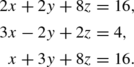
Find the solution sets of the following systems of equations, and sketch the corresponding graphs.

$$\begin{array}{l@{\quad}rcl@{\qquad}l@{\quad}rcl}(\mathrm{i}) & 3x - 2y & = & 4, &(\mathrm{ii}) & 2x - y & = & 1, \\& 3x - 2y & = & -1; & &-4x + 2y &= & -2.\end{array}$$

Solution

In case (i), 3x−2y cannot equal both 4 and −1, so there are no solutions, and the solution set is empty. In system (ii), whenever the first equation is true, the second will be true also: each side of the second equation is (−2) times the corresponding side of the first one. The solution set could be written {(x,y)∣2x−y=1∣x∈ℝ} or {(x,2x−1)∣x∈ℝ}. The graphs are

Your Turn

Find the solution sets of the following systems of equations, and sketch the corresponding graphs:

$$\begin{array}{rcl@{\qquad}rcl}2x + 2y & = & 3, & x - 2y & = & 1, \\[3pt]2x + 2y & = & 4; & 2x - 4y & = & 2.\end{array}$$

5.2.2 Solution by Elimination

Consider the system of equations

$$\begin{array}{rcl}x + y & = & 8, \\[3pt]x - y & = & 4.\end{array} $$

(5.1)

If x+y=8 is true, then

$$x + y + c = 8 + c$$

will be true for any real quantity c. In particular,

$$ x + y + (x - y) = 8 + (x - y), $$

(5.2)

whatever the values of x and y may be. Now suppose x and y form a solution of (5.1). Then x−y=4, so we could write 4 instead of (x−y) on either side of (5.2). Let’s make this change on the right side only. We have

$$x + y + (x - y) = 8 + 4 = 12,$$

so 2x=12 and x=6. So any solution of (5.1) must have x=6. Then (5.2) tells us 6−y=4, so y=6−4=2. The only possible solution is x=6,y=2. If you check, you’ll see that these values make both equations in (5.1) true, so we have solved the system.

The key to this method was the way the two terms y and −y eliminated each other. For this reason we say we solved the equations by elimination, and say y was eliminated. The technique is sometimes called the addition (or subtraction) method because it can be described like this: we add the left-hand side of the second equation to the left-hand side of the first, and then add the right-hand side of the second equation to the right-hand side of the first. Usually we simply say we add the second equation to the first.

We could also have eliminated x. Starting from the first equation in (5.1), we could write

$$x + y - (x - y) = 8 - (x - y),$$

so

$$x + y - x + y = 8 - 4 = 4,$$

2y=4, y=2, and we then deduce x=6 from the original equations.

Sample Problem 5.9

Solve the following equations by elimination:

Solution

We would like to eliminate y from the first equation. The coefficient of y in the second equation is 2, not 4. To get around this problem, we could multiply both sides of the second equation by 2. This will not change the solution set; we could multiply by any constant other than 0. In other words, we proceed to solve the equations

Adding the equations, we find

$$16x = 16,$$

so x=1. Substituting this back into the second equation we get

$$5 \cdot1 - 2y = 3,$$

so y=1, and the solution is (x,y)=(1,1). We usually say we added 2⋅(equation 2) to (equation 1), and do not bother to write down the new set of equations.

Your Turn

Solve the following equations by elimination:

Sample Problem 5.10

Solve the following equations by elimination:

Solution

In order to eliminate y from the first equation, we multiply the second equation by $\frac{3}{2}$, obtaining

$$\frac{9}{2}x - 3y = \frac{15}{2}$$

and add this to the first equation, getting

substituting back we get 2y=4, or y=2.

5.2.3 Systems of Three or More Equations

These techniques can be applied to any number of equations in any number of variables. However, more variability occurs in dependent systems when there are more than two equations.

Sample Problem 5.11

Solve the following equations by elimination:

Solution

We eliminate x from the first and third equations. We add −3 times the second equation to the first equation and −5 times the second equation to the third equation; those two equations become

So we get two copies of the same equation. Its solution is y=1+z, where z can be any real number. When we substitute this into the original second equation, we get

$$\begin{array}{rcl}x - 3(1+z) + 3z & = & -2,\\[4pt]x - 3 &= & -2.\end{array}$$

So x=1, and the solution is

$$(x,y,z) \in\bigl\{(1, 1+z, z) \mid z \in \mathbb{R}\bigr\}.$$

The following examples show two further possible forms of dependent solution. Of course, a set of three equations can also be inconsistent (no solutions) or independent (precisely one solution).

Sample Problem 5.12

Solve the following equations by elimination:

$$\begin{array}{rcl}x + 2y + z & = & 8,\\[3pt]2x + y - z & = & 7,\\[3pt]3x - y - 4z & = & 3.\end{array}$$

Solution

We eliminate z from the second and third equations by adding the first equation to the second equation and 4 times the first equation to the third equation; those two equations become

$$\begin{array}{rcl}3x + 3y & = & 15, \\[3pt]7x + 7y & = & 35.\end{array}$$

So we get x=5−y, where y can be any real number. When we substitute this into the original first equation, we get

$$\begin{array}{rcl}(5-y) + 2y + z & = & 8,\\[3pt]y + z & = & 3.\end{array}$$

So z=3−y, and the solution is

$$(x,y,z) \in\bigl\{(5-y, y, 3-y) \mid y \in \mathbb{R}\bigr\}.$$

Observe that we expressed both x and z in terms of the same variable, y.

Sample Problem 5.13

Solve the following equations by elimination:

$$\begin{array}{rcl}2x + 4y - 6z & = & 6, \\[3pt]x + 2y - 3z & = & 3, \\ [3pt]-3x - 6y + 9z & = & -9.\end{array}$$

Solution

We eliminate x from the first and third equations. We add −2 times the second equation to the first equation and 3 times the second equation to the third equation; those two equations both give the form 0=0: both sides are completely eliminated. It follows that any x, y, and z satisfying the original second equation will also satisfy the others. The solution is

$$(x,y,z) \in\bigl\{(3-2y + 3z, y, z) \mid y \in \mathbb{R}, z \in \mathbb{R}\bigr\}.$$

Your Turn

Solve the following equations by elimination:

$$\begin{array}{rcl}3x + 2y - z & = & 7, \\[3pt]x + y &= & 3, \\[3pt]2x - y - 3z & = & 0.\end{array}$$

The same solution technique can be applied to the case where there are three unknowns but only two equations. In this case, an independent solution is impossible.

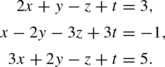
Sample Problem 5.14

Solve the following equations by elimination:

$$\begin{array}{rcl}2x + 3y + 2z & = & 4,\\[3pt]x + y - z & = & 2.\end{array}$$

Solution

We eliminate z from the second equation by adding the first equation to twice the second equation, obtaining

$$4x + 4y = 8.$$

We have x=2−y, where y can be any real number. Substituting this into the original first equation yields

$$\begin{array}{rcl}2(2-y) + 3y + 2z & = & 4,\\[3pt]y + 2z & = & 0.\end{array}$$

So $z = -{\textstyle{\frac{1}{2}} }y$, and the solution is

$$(x,y,z) \in\biggl\{\biggl(2-y, y, -\frac{1}{2} y\biggr) \biggm{|} y \in \mathbb{R}\biggr\}.$$

Your Turn

Solve the following equations by elimination:

$$\begin{array}{rcl}x + 2y - z & = & 5, \\[3pt]2x - 3y - z & = & 3.\end{array}$$

Exercises 5.2 A

1.
In each part, find the complete solution of the system of two linear equations, by substitution.
1. (i)
  $\begin{array}[t]{rcl}2x + y & = & 12, \\[3pt]3x - y & = & 13;\end{array}$
2. (ii)
  $\begin{array}[t]{rcl}x + 5y & = & 11, \\[3pt]x + 2y & = & 2;\end{array}$
3. (iii)
  $\begin{array}[t]{rcl}5x + 3y & = & 7, \\[3pt]3x - y & = & 0;\end{array}$
4. (iv)
  $\begin{array}[t]{rcl}3x - 4y & = & 4, \\[3pt]x + 2y & = & 3;\end{array}$
5. (v)
  $\begin{array}[t]{rcl}7x - 2y & = & 5,\\[3pt]12x - 4y & = & 4;\end{array}$
6. (vi)
  $\begin{array}[t]{rcl}-2x + 5y & = & 4, \\[3pt]2x - 3y & = & -2;\end{array}$
7. (vii)
  $\begin{array}[t]{rcl}3x - y & = & 5, \\[3pt]4x - 2y & = & 6;\end{array}$
8. (viii)
  $\begin{array}[t]{rcl}\displaystyle \frac{1}{2} x + 3y & = & -1, \\[8pt]3x - 2y & = & 2;\end{array}$
9. (ix)
  $\begin{array}[t]{rcl}5x + 3y & = & 8, \\[3pt]3x + y & = & 0;\end{array}$
10. (x)
  $\begin{array}[t]{rcl}2x + y & = & -1, \\[3pt]2x - y & = & -3.\end{array}$
2.
In each of the parts of Exercise 1, find the complete solution of the system of two linear equations by elimination.
3.
In the following problems, say whether the equations are inconsistent, dependent or independent. If they are consistent, write down the solution.
1. (i)
  $\begin{array}[t]{rcl}3x - 2y & = & 0, \\[3pt]6x - 4y & = & 9;\end{array}$
2. (ii)
  $\begin{array}[t]{rcl}4x - 5y & = & 0, \\[3pt] 2x - 3y & = & -2;\end{array}$
3. (iii)
  $\begin{array}[t]{rcl} 3x - 2y & = & 0, \\[3pt] 2x + 6y & = & 11;\end{array}$
4. (iv)
  $\begin{array}[t]{rcl}4x + 2y & = & 1, \\[5pt]-2x + 3y & = & -\displaystyle \frac{1}{2};\end{array}$
5. (v)
  $\begin{array}[t]{rcl} 4x - 2y & = & 8, \\[3pt] 2x - y & = & 4;\end{array}$
6. (vi)
  $\begin{array}[t]{rcl}4x - 2y & = & 4, \\[3pt] -2x + y & = & -2;\end{array}$
7. (vii)
  $\begin{array}[t]{rcl} 6x + 4y & = & 9, \\[3pt] 3x + 2y & = & 4;\end{array}$
8. (viii)
  $\begin{array}[t]{rcl}3 x + y & = & 30, \\[3pt]x + 2 y & = & 12;\end{array}$
9. (ix)
  $\begin{array}[t]{rcl} x + 2y & = & 5, \\[3pt]10x - y & = & 6;\end{array}$
10. (x)
  $\begin{array}[t]{rcl}10x - 16y & = & 2, \\[3pt]-15x + 24y & = & -3.\end{array}$
4.
In the following problems, say whether the equations are inconsistent, dependent or independent. If they are consistent, write down the solution.
1. (i)
  $\begin{array}[t]{rcl}x + y + z & = & 4, \\[3pt]2x - y + z & = & 3, \\[3pt]x + 2y + 3z & = & 4;\end{array}$
2. (ii)
  $\begin{array}[t]{rcl}x + 4y - 3z & = & -24, \\[3pt]3x - y + 3z & = & 36, \\[3pt]x + y + 6z & = & 3;\end{array}$
3. (iii)
  $\begin{array}[t]{rcl}x - y - z & = & 1, \\[3pt]x - 2y + 3z & = & 4, \\[3pt]3x - 2y - 7z & = & 0;\end{array}$
4. (iv)
  $\begin{array}[t]{rcl}2x - 2y - 3z & = & 6, \\[3pt]4x - 3y - 2z & = & 0, \\[3pt]2x - 3y - 7z & = & -1;\end{array}$
5. (v)
  $\begin{array}[t]{rcl}3x - 2y + 2z & = & 10, \\[3pt]x - 2y + 3z & = & 7, \\[3pt]2x + y + z & = & 4;\end{array}$
6. (vi)
  $\begin{array}[t]{rcl}x - y - z & = & 1, \\[3pt]x - 2y + 3z & = & 4, \\[3pt]2x - y - 6z & = & -1;\end{array}$
7. (vii)
  $\begin{array}[t]{rcl}x + y - z & = & -1, \\[3pt]2x - 2y - 3z & = & 5, \\[3pt]4x - 3y + 2z & = & 16;\end{array}$
8. (viii)
  $\begin{array}[t]{rcl}x - y - z & = & 1, \\[3pt]2x + 3y + z & = & 2, \\[3pt]3x + 2y & = & 0;\end{array}$
9. (ix)
  $\begin{array}[t]{rcl}x - y & = & 1, \\[3pt]2x - 3y + z & = & 6;\end{array}$
10. (x)
  $\begin{array}[t]{rcl}3x + y - 6z & = & 4, \\[3pt]2x - y + z & = & 1;\end{array}$
11. (xi)
  $\begin{array}[t]{rcl}x - y + z & = & 20, \\[3pt]x + y + z & = & 10, \\[3pt]2x + y & = & 17;\end{array}$
12. (xii)
  $\begin{array}[t]{rcl}2x - 2y - z & = & 0, \\[3pt]2x - y + 2z & = & 4, \\[3pt]2x + 3y + z & = & 20;\end{array}$
13. (xiii)
  $\begin{array}[t]{rcl}x + z & = & 2, \\[3pt]x + y & = & 0, \\[3pt]y + z & = & 2;\end{array}$
14. (xiv)
  $\begin{array}[t]{rcl}x - 2y + 2z & = & 2, \\[3pt]2x - 3y + 3z & = & 2, \\[3pt]5x - 8y + 8z & = & 7.\end{array}$

Exercises 5.2 B

1.
In each part, find the complete solution of the system of two linear equations, by substitution.
1. (i)
  $\begin{array}[t]{rcl}3x - 2y & = & 10,\\[3pt] 2x - 3y & = & 15;\end{array}$
2. (ii)
  $\begin{array}[t]{rcl}\displaystyle \frac{1}{2} x + 3y & = & -2, \\[8pt]x - 2y & = & 8;\end{array}$
3. (iii)
  $\begin{array}[t]{rcl}7x + 4y & = & 2, \\[3pt] 3x - 2y & = & 0;\end{array}$
4. (iv)
  $\begin{array}[t]{rcl}2x + y & = & -1, \\[3pt] 2x - y & = & -3;\end{array}$
5. (v)
  $\begin{array}[t]{rcl}5x + 3y & = & 4, \\[3pt] 3x - y & = & 1;\end{array}$
6. (vi)
  $\begin{array}[t]{rcl} 11x + 7y & = & 1, \\[3pt] -2x - 3y &= & 5;\end{array}$
7. (vii)
  $\begin{array}[t]{rcl}2x + 3y & = & 8, \\[3pt] -2x - 2y & = & -4;\end{array}$
8. (viii)
  $\begin{array}[t]{rcl}3x - 2y & = & 5, \\[3pt] 2x + 3y & = & 12;\end{array}$
9. (ix)
  $\begin{array}[t]{rcl} 5x + 7y & = & -1, \\[3pt] 4x + 7y & = & 2;\end{array}$
10. (x)
  $\begin{array}[t]{rcl} 3x - 5y & = & 0, \\[5pt]2x + 3y & = & \displaystyle \frac {38}{15};\end{array}$
11. (xi)
  $\begin{array}[t]{rcl} 3x + 2y & = & 10,\\[3pt] 2x - 3y & = & -4;\end{array}$
12. (xii)
  $\begin{array}[t]{rcl}4x - 3y & = & 11, \\[3pt]2x + 2y & = & 16;\end{array}$
13. (xiii)
  $\begin{array}[t]{rcl} 6x - 3y & = & 1, \\[3pt] 8x + 5y & = & 7;\end{array}$
14. (xiv)
  $\begin{array}[t]{rcl}3x + 11y & = & 5, \\[3pt]5x + 15y & = & 10;\end{array}$
15. (xv)
  $\begin{array}[t]{rcl}2x + 2y & = & 12, \\[3pt] 5x - 3y & = & 14;\end{array}$
16. (xvi)
  $\begin{array}[t]{rcl}2x + 3y & = & 2, \\[3pt] 2x - y & = & -6.\end{array}$
2.
In each of the parts of Exercise 1, find the complete solution of the system of two linear equations by elimination.
3.
In the following problems, say whether the equations are inconsistent, dependent or independent. If they are consistent, write down the solution.
1. (i)
  $\begin{array}[t]{rcl} 4x - 3y & = & 15, \\[3pt] 2x + 5y & = & 1;\end{array}$
2. (ii)
  $\begin{array}[t]{rcl} 2x - 3y & = & 1, \\[3pt] 3x +3y & = & 9;\end{array}$
3. (iii)
  $\begin{array}[t]{rcl} 2x - 2y & = & 6, \\[3pt] 3x - 3y & = & 7;\end{array}$
4. (iv)
  $\begin{array}[t]{rcl}3x - 4y & = & 0, \\[3pt]6x - 8y & = & 7;\end{array}$
5. (v)
  $\begin{array}[t]{rcl} 7x - 4y & = & 2, \\[3pt] 4x - 3y & = & -1;\end{array}$
6. (vi)
  $\begin{array}[t]{rcl} 11x - 7y & = & 1, \\[3pt]3x + 3y & = & 15;\end{array}$
7. (vii)
  $\begin{array}[t]{rcl} 6x + 4y & = & 8, \\[3pt] 3x + 2y & = & 4;\end{array}$
8. (viii)
  $\begin{array}[t]{rcl}\displaystyle \frac{1}{2} x - y & = & 0, \\[8pt]\displaystyle x + \frac{1}{2} y & = & 5;\end{array}$
9. (ix)
  $\begin{array}[t]{rcl} 4x + 3y & = & 1, \\[3pt]-2x + 5y & = & -7;\end{array}$
10. (x)
  $\begin{array}[t]{rcl}10x - 14y & = & 2, \\[3pt]-15x + 21y & = & -3;\end{array}$
11. (xi)
  $\begin{array}[t]{rcl} 2x + 3y & = & 12, \\[3pt] x - 3y & = & -3;\end{array}$
12. (xii)
  $\begin{array}[t]{rcl} x - y & = & 5, \\[3pt] x + y & = & 9;\end{array}$
13. (xiii)
  $\begin{array}[t]{rcl} x - 2y & = & 3, \\[3pt] 3x - 6y & = & 9;\end{array}$
14. (xiv)
  $\begin{array}[t]{rcl}4x - 6y & = & 0, \\[3pt]6x - 9y & = & 7;\end{array}$
15. (xv)
  $\begin{array}[t]{rcl} 3x - 2y & = & 6, \\[3pt] x + 2y & = & 6;\end{array}$
16. (xvi)
  $\begin{array}[t]{rcl} x + 2y & = & 5, \\[3pt] 2x + 3y & = & 4.\end{array}$
4.
In the following problems, say whether the equations are inconsistent, dependent or independent. If they are consistent, write down the solution.
1. (i)
  $\begin{array}[t]{rcl}x - z & = & 2, \\[3pt]x - 2y + z & = & -4, \\[3pt]2x + y - 3z & = & 7;\end{array}$
2. (ii)
  $\begin{array}[t]{rcl}x + 2y - z & = & 6, \\[3pt]2x + 4y - 2z & = & 12, \\[3pt]2x + 7y + z & = & 24;\end{array}$
3. (iii)
  $\begin{array}[t]{rcl}x + z & = & 2, \\[3pt]x + y & = & 0, \\[3pt]y + z & = & 0;\end{array}$
4. (iv)
  $\begin{array}[t]{rcl}3x - 2y + 2z & = & 2, \\[3pt]2x - 4y + 3z & = & 2, \\[3pt]5x + 2y & = & 4;\end{array}$
5. (v)
  $\begin{array}[t]{rcl}x + 2y + z & = & 2, \\[3pt]3x + 6y + 3z & = & 6, \\[3pt]2x + 4y + 2z & = & 4;\end{array}$
6. (vi)
  $\begin{array}[t]{rcl}x - y - z & = & 9, \\[3pt]x + y + 3z & = & -5;\end{array}$
7. (vii)
  $\begin{array}[t]{rcl}2x - 2y - z & = & 0, \\[3pt]2x - y + 2z & = & 2, \\[3pt]2x + 3y + z & = & 10;\end{array}$
8. (viii)
  $\begin{array}[t]{rcl}2x + y - z & = & 1, \\[3pt]4x + 2y + 2z & = & 0, \\[3pt]2x - y + z & = & 6;\end{array}$
9. (ix)
  $\begin{array}[t]{rcl}3x - y + 4z & = & 5, \\[3pt]x - 2y + 3z & = & 7, \\[3pt]2x + y + z & = & 4;\end{array}$
10. (x)
  $\begin{array}[t]{rcl}x - 2y + 2z & = & 3, \\[3pt]2x - 4y + z & = & 3, \\[3pt]4x - 8y + 3z & = & 7;\end{array}$
11. (xi)
  $\begin{array}[t]{rcl}2x - y + z & = & 9, \\[3pt]x + y + z & = & 9, \\[3pt]x - y + z & = & 3;\end{array}$
12. (xii)
  $\begin{array}[t]{rcl}x + y - z & = & 8, \\[3pt]x + 4y + z & = & 12, \\[3pt]x - 2y + z & = & -4;\end{array}$
13. (xiii)
  $\begin{array}[t]{rcl}4x - 4y + 2z & = & 10, \\[3pt]2x + y - z & = & -6, \\[3pt]6x - 7y + z & = & 12;\end{array}$
14. (xiv)
  $\begin{array}[t]{rcl}3x - 4y + 11z & = & 6, \\[3pt]2x - 5y + 12z & = & 4;\end{array}$
15. (xv)
  $\begin{array}[t]{rcl}x + y + 2z & = & 20, \\[3pt]x - y - 2z & = & 6, \\[3pt]x + y + z & = & 40;\end{array}$
16. (xvi)
  $\begin{array}[t]{rcl}x + y + 2z & = & 4, \\[3pt]x + y - 2z & = & 0, \\[3pt]x + y + 3z & = & 5;\end{array}$
17. (xvii)
  $\begin{array}[t]{rcl}x + 2y - z & = & 6, \\[3pt]2x + 4y + 2z & = & 8, \\[3pt]2x + 3y + z & = & 7;\end{array}$
18. (xviii)
  $\begin{array}[t]{rcl}x + 2y + z & = & 4, \\[3pt]x + y + z & = & -4, \\[3pt]2x - 2y + 2z & = & 8;\end{array}$
19. (xix)
  $\begin{array}[t]{rcl}x + y + z & = & 6, \\[3pt]x - y + 2z & = & 12, \\[3pt]2x + y + z & = & 1;\end{array}$
20. (xx)
  $\begin{array}[t]{rcl}x - 2y + z & = & 3, \\[3pt]2x - 4y + 3z & = & 7.\end{array}$

5.3 Formal Solution of Systems of Equations

5.3.1 The Augmented Matrix

In this section, we formalize the process of solving a system of linear equations by substitution. In order to talk about a system of m equations in n variables, we use subscripts. We suppose the variables are x ₁,x ₂,…,x _n, and suppose the ith equation to be

$$a_{i1}x_1 + a_{i2}x_2 + \cdots+ a_{in}x_n = b_i,$$

where a ₁₁, a ₁₂,…,a _mn, b ₁,…,b _m are some constants.

We define the augmented matrix of a system to be the following array of numbers:

$$\left[\begin{array}{c@{\quad}c@{\quad}c@{\quad}c@{\ }|@{\ }c}a_{11} & a_{12} & \cdots& a_{1n} & b_1 \\a_{21} & a_{22} & \cdots& a_{2n} & b_2 \\\vdots& \vdots& \ddots& \vdots& \vdots\\a_{m1} & a_{m2} & \cdots& a_{mn} & b_m\end{array}\right].$$

The vertical line indicates the division between the two types of element, the coefficients on the left and the constant terms on the right. The horizontal lists of numbers are called rows and the vertical lists are called columns. The ith row corresponds to the ith equation; the jth column corresponds to the jth variable when 1≤j≤n, while column n+1 corresponds to the list of constant terms of the equations. The number lying in the ith row and the jth column is called the (i,j) element of the augmented matrix.

Augmented matrices are a special case of more general matrices, or rectangular arrays of numbers, and we shall discuss the general case in the next section. Many of the ideas and notations will be repeated there, but you will find them to be consistent with this section.

Sample Problem 5.15

Write down the augmented matrix of the system

What is its (2,3) element?

Solution

$$\left[\begin{array}{c@{\quad}c@{\quad}c@{\ }|@{\ }c} 2&4&-3&4 \\ 0&-2&4&6 \\ 1&-1&4&10\end{array}\right].$$

The (2,3) element equals 4.

Your Turn

Write down the augmented matrix of the system

What is its (2,2) element?

The first step in solving a set of equations is to select a variable to eliminate. This is equivalent to choosing a column in the augmented matrix and selecting a row—an equation—to use for substitution. We say that we are operating on the element in that row and column. The only requirement is that the matrix has a non-zero entry in that row and column.

To illustrate this, consider the system in Sample Problem 5.15. Let us choose row 3, column 1, representing variable x in the first equation. It will be convenient to interchange rows 1 and 3, so that we are operating on the (1,1) entry. This is equivalent to rewriting the equations in a different order. The matrix is now

$$\left[\begin{array}{c@{\quad}c@{\quad}c@{\ }|@{\ }c} 1&-1&4&10 \\ 0&-2&4&6 \\ 2&4&-3&4\end{array}\right]\quad \begin{array}{l} R1 \gets R3, \\\\ R3 \gets R1,\end{array}$$

where the annotations mean the new row 1 is the old row 3 and the new row 3 is the old row 1.

Now substitute for x in the other equations. No action is required in the second equation, but x must be eliminated from the third. So we subtract twice the first row from the third row. This yields precisely the equation we would get if we used equation 1 to substitute for x in equation 3, but for consistency we have kept all the variables on the left-hand side of the equation. The augmented matrix becomes

$$\left[\begin{array}{c@{\quad}c@{\quad}c@{\ }|@{\ }c} 1&-1&4&10 \\ 0&-2&4&6 \\ 0&6&-11&-16\end{array}\right]\quad \begin{array}{l}\\\\ R3 \gets R3 - 2R1,\end{array}$$

where the legend means the new row 3 is (the old row 3) −2(the old row 1). (When we say old we are referring to the preceding augmented matrix, not to the original one.)

Now multiply row 2 by $- {\textstyle{\frac{1}{2}} }$. Then eliminate the 6y from the third equation. The result is

$$\left[\begin{array}{c@{\quad}c@{\quad}c@{\ }|@{\ }c} 1&-1&4&10 \\ 0&1&-2&-3 \\ 0&0&1&2\end{array}\right]\quad \begin{array}{l}\\ R2 \gets {\textstyle{\frac{1}{2}} }R2, \\R3 \gets R3 - 6({\textstyle{\frac{1}{2}} }R2) .\end{array}$$

This could have been broken into two steps.

So far we have done the equivalent of substituting in the later equations. Now we substitute back to find the values. We know from the third equation that z=3. To substitute this in the earlier equations, we add twice row 3 to row 2 and subtract four times row 3 from row 1:

$$\left[\begin{array}{c@{\quad}c@{\quad}c@{\ }|@{\ }c} 1&-1&0& 2 \\ 0& 1&0& 1 \\ 0& 0&1& 2\end{array}\right]\quad \begin{array}{r}R1 \gets R1 - 4 R3, \\R2 \gets R2 + 2 R3. \\\\\end{array}$$

Next add row 2 to row 1:

$$\left[\begin{array}{c@{\quad}c@{\quad}c@{\ }|@{\ }c}1& 0&0& 3 \\0& 1&0& 1 \\0& 0&1& 2\end{array}\right]\quad \begin{array}{l}R1 \gets R1 + R2.\\\\\\\end{array}$$

The resulting array can be translated into the equations

$$x = 3,\qquad y = 1,\qquad z = 2.$$

5.3.2 Elementary Operations

In our example, we used three operations:

E1::: exchange two rows of the matrix;
E2::: multiply a row by a (non-zero) constant;
E3::: add a multiple of one row to another row.

We shall call these the elementary row operations. Their importance comes from the following fact:

Theorem 17

Suppose P is the augmented matrix of a system of linear equations, and Q is obtained from P by a sequence of elementary row operations. Then the system of equations corresponding to Q has the same solutions as the system corresponding to P.

It is clear that repeated application of the three elementary operations to the augmented matrix will provide a solution. So we can solve systems of linear equations by the following technique.

Stage 1.

1. Find the leftmost column in the matrix of coefficients that contains a non-zero element, say column j. Use E1 to make the row containing this element into the first row, and E2 to convert its leftmost non-zero element to 1. This is called a leading 1. Then use E3 to change all entries below the leading 1 to zero. That is, if the (i,j) entry is a _ij, then subtract a _ij⋅(row 1) from row j.

At this stage we say column j is processed. Processed columns are not disturbed in the first stage.

2. Find the leftmost unprocessed column in the augmented matrix that contains a non-zero element, say column k. Use E1 to make this row the first row under the processed row(s), and E2 to convert its leftmost non-zero element to 1, another leading 1. Use E3 to change all entries below the leading 1 to zero (but do not change the processed row or rows). Now column k is also processed.

3. If you have not either reached the last column of coefficients (the vertical line) or the bottom of the matrix, go back to step 2, make another leading 1 and proceed from there.

Stage 2.

4. Choose the bottom-most leading 1 and eliminate all elements above it in its column by use of E3. Do the same to the next leading 1 up, then the next, until you reach the top.

The process is now finished.

Sample Problem 5.16

Solve the system

by row operations.

Solution

The augmented matrix is

$$\left[\begin{array}{c@{\quad}c@{\quad}c@{\ }|@{\ }c}2& 2&4& 0 \\[-1pt]3& -1& 2& 1 \\[-1pt]8&0 &8& 2\end{array}\right].$$

At step 1, we choose the element in the (1,1) position and divide row 1 by 2:

$$\left[\begin{array}{c@{\quad}c@{\quad}c@{\ }|@{\ }c}1& 1&2& 0 \\[-1pt]3& -1& 2& 1 \\[-1pt]8&0 &8& 2\end{array}\right]\quad \begin{array}{l} R1 \gets {\textstyle{\frac{1}{2}} }R1 \quad \mbox{(using E2).} \\\\\\\end{array}$$

Then we eliminate the rest of column 1:

$$\left[\begin{array}{c@{\quad}c@{\quad}c@{\ }|@{\ }c}1& 1&2& 0 \\[-1pt]0& -4&-4& 1 \\[-1pt]0&-8&-8& 2\end{array}\right]\quad \begin{array}{l}\\ R2 \gets R2 - 3 \times R1 \quad \mbox{(using E3)}, \\[-1pt]R3 \gets R3 - 8 \times R1 \quad \mbox{(using E3)}. \\\end{array}$$

In step 2, we choose the (2,2) position and divide by −4, then eliminate the entries below the (2,2) position, obtaining successively

There are no further numbers available for leading 1’s, so we move to step 4. We use the (2,2) element:

$$\left[\begin{array}{c@{\quad}c@{\quad}c@{\ }|@{\ }c} 1& 0&1& {\textstyle{\frac{1}{4}} }\\0& 1&1& -{\textstyle{\frac{1}{4}} }\\0& 0& 0& 0\end{array}\right]\quad \begin{array}{l} R1 \gets R1 - R2 \quad \mbox{(using E3).} \\\\\ \end{array}$$

The process is finished. There is no restriction on z. The final augmented matrix converts to the system

(the third equation can be ignored), and the final solution could be expressed as

$$x = \frac{1}{4}- z, \qquad y = -\frac{1}{4}- z,\qquad \mbox{any real number } z.$$

Notice that the sequence of calculations is completely determined by the matrix of coefficients, the left-hand part of the augmented matrix.

If the column corresponding to a variable receives a leading 1, we shall call that variable dependent; the others are independent. One standard way of recording the answer is to give an equation for each dependent variable, with a constant and the independent variables on the right; the independent variables take any real number value. Another way to express the above solution would be to use set notation $\{{\textstyle{\frac{1}{4}} }- z,\allowbreak -{\textstyle{\frac{1}{4}} }- z,z) \mid z\in \mathbb{R}\}$, or perhaps $\{t + {\textstyle{\frac{1}{4}} }, t, -{\textstyle{\frac{1}{4}} }, - t) \mid t \in \mathbb{R}\}$. In this case, t is called a parameter.

Sometimes there will be no solution to a system of equations. The equations are then called inconsistent.

Sample Problem 5.17

Solve the system

Solution

The augmented matrix is

$$\left[\begin{array}{c@{\quad}c@{\quad}c@{\ }|@{\ }c} 2& 2&4& 0 \\ 3& -1& 2& 1 \\ 8&0&8& 3\end{array}\right].$$

The left-hand part of this equation is the same as in Sample Problem 5.16, so we go through the same steps, making the appropriate changes to the right-hand column. At the end of Stage 1, we have

$$\left[\begin{array}{c@{\quad}c@{\quad}c@{\ }|@{\ }c}1& 1&2& 0 \\0& 1&1& -{\textstyle{\frac{1}{4}} }\\0& 0& 0& 1\end{array}\right].$$

When we convert back to equations, the third row gives the equation

$$0 = 1,$$

which is impossible. No values of x,y and z make this true, so the equations are inconsistent. There is no need to implement Stage 2.

In set-theoretic terms, we could report that the solution set is ∅.

Exercises 5.3 A

1.
In each case, the augmented matrix of a system of equations is shown. Assuming the variables are x,y,z, what is the solution of the system?
1. (i)
  $\left[\begin{array}{c@{\quad}c@{\quad}c@{\ }|@{\ }c} 1& 0&0& 3 \\ 0& 1&0& 1 \\ 0& 0& 0&0\end{array}\right]$;
2. (ii)
  $\left[\begin{array}{c@{\quad}c@{\quad}c@{\ }|@{\ }c} 1& 0&1& 2 \\ 0& 1&-1& 1 \\ 0& 0& 0& 0\end{array}\right]$;
3. (iii)
  $\left[\begin{array}{c@{\quad}c@{\quad}c@{\ }|@{\ }c} 1& 0&1& 2 \\ 0& 1&2& 1 \\ 0& 0& 0& 2\end{array}\right]$;
4. (iv)
  $\left[\begin{array}{c@{\quad}c@{\quad}c@{\ }|@{\ }c} 1& 0&1& 2 \\ 0& 1&1& 1 \\ 0& 0& 0& 1\end{array}\right]$;
5. (v)
  $\left[\begin{array}{c@{\quad}c@{\quad}c@{\ }|@{\ }c} 1& 0&0& 2 \\ 0& 1&0& 2 \\ 0& 0& 0& 1\end{array}\right]$;
6. (vi)
  $\left[\begin{array}{c@{\quad}c@{\quad}c@{\ }|@{\ }c} 1& 0&0& 2 \\ 0& 1&0& 2 \\ 0& 0& 0& 0\end{array}\right]$;
7. (vii)
  $\left[\begin{array}{c@{\quad}c@{\quad}c@{\ }|@{\ }c} 1& 1&1& 4 \\ -1&2&1& -1 \\ 3& 2& 4& 6\end{array}\right]$;
8. (viii)
  $\left[\begin{array}{c@{\quad}c@{\quad}c@{\ }|@{\ }c} 4& 3& 1&11 \\ 2&-2& 4& 2 \\ 1& 3&-2& 5\end{array}\right]$;
9. (ix)
  $\left[\begin{array}{c@{\quad}c@{\quad}c@{\ }|@{\ }c} 1& 0&2& 2 \\ 0& 1&-1& 1 \\ 0& 0& 0& 2\end{array}\right]$;
10. (x)
  $\left[\begin{array}{c@{\quad}c@{\quad}c@{\ }|@{\ }c} 1& 0&2& 2 \\ 0& 1&2& 1 \\ 0& 0& 1& 1\end{array}\right]$.
2.
Solve the following systems of equations:
1. (i)
  $\begin{array}[t]{rcl} 2x + 6y & = & 6, \\4x + 11y & = &10;\end{array}$
2. (ii)
  $\begin{array}[t]{rcl} 2x + 3y & = & 5, \\4x + 6y & = &10;\end{array}$
3. (iii)
  $\begin{array}[t]{rcl} 3x - y & = & 4, \\6x - 2y & = & 2;\end{array}$
4. (iv)
  $\begin{array}[t]{rcl} x - 2y & = & 4, \\-3x - 4y & = &-2, \\2x + 3y & = & 1.\end{array}$
3.
Solve the following systems of equations:
1. (i)
  $\begin{array}[t]{rcl} x + 2y + z & = & 3, \\x + y - 2z & = & 2;\end{array}$
2. (ii)
  $\begin{array}[t]{rcl} 2x + 2z & = & 2, \\x + 2y + 6z & = & 3, \\2x - 2y & = & 1;\end{array}$
3. (iii)
  $\begin{array}[t]{rcl} x + 2y + z & = & -1, \\2x + 3y - 2z & = & 7, \\-2x + 2y - 3z & = & -2;\end{array}$
4. (iv)
  $\begin{array}[t]{rcl} x + y & = & 2, \\x - y + 5z & = & 3, \\-3x - 3y + 2z & = & -6.\end{array}$
4.
Solve the following systems of equations:
1. (i)
  $\begin{array}[t]{rcl} 3x - 2y - 8z + 7t & = & 1, \\x + y - z - t & = & 3, \\x - y - 3z + 3t & = & -1;\end{array}$
2. (ii)
  $\begin{array}[t]{rcl} x + 2y + 3z + 4t & = & 8, \\x - 3y + 4z + 4t & = & 8, \\2x - 2y - z + t & = & -3, \\x - 7y - 7z - 3t & = & -11.\end{array}$

Exercises 5.3 B

1.
In each case, the augmented matrix of a system of equations is shown. Assuming the variables are x,y,z, what is the solution of the system?
1. (i)
  $\left[\begin{array}{c@{\quad}c@{\quad}c@{\ }|@{\ }c} 1& 0&0& -1 \\ 0& 1&0& -1 \\ 0& 0& 1& -1\end{array}\right]$;
2. (ii)
  $\left[\begin{array}{c@{\quad}c@{\quad}c@{\ }|@{\ }c} 1& 0&0& 3 \\ 0& 1&0& 1 \\ 0& 0& 1& 2\end{array}\right]$;
3. (iii)
  $\left[\begin{array}{c@{\quad}c@{\quad}c@{\ }|@{\ }c} 1& 0&0& 4 \\ 0& 1&0& 1 \\ 0& 0& 1& 1\end{array}\right]$;
4. (iv)
  $\left[\begin{array}{c@{\quad}c@{\quad}c@{\ }|@{\ }c} 1& 0&0& 2 \\ 0& 0& 1& 1 \\ 0& 0& 0& 0\end{array}\right]$;
5. (v)
  $\left[\begin{array}{c@{\quad}c@{\quad}c@{\ }|@{\ }c} 1& 1&0& 2 \\ 0& 0&1&-1 \\ 0& 0&0& 0 \\0& 0& 0& 0\end{array}\right]$;
6. (vi)
  $\left[\begin{array}{c@{\quad}c@{\quad}c@{\ }|@{\ }c} 1& 0&0& 2 \\ 0& 1&0& 1 \\ 0& 0&1& 1 \\0& 0& 0& 1\end{array}\right]$;
7. (vii)
  $\left[\begin{array}{c@{\quad}c@{\quad}c@{\ }|@{\ }c} 1& 1&1& 3 \\ -1&1&1& 1 \\ 1& 2& 3& 6\end{array}\right]$;
8. (viii)
  $\left[\begin{array}{c@{\quad}c@{\quad}c@{\ }|@{\ }c} 2& 1& 1&5 \\ 2&-1& 3& 3 \\ 4& 1& 3& 9\end{array}\right]$;
9. (ix)
  $\left[\begin{array}{c@{\quad}c@{\quad}c@{\ }|@{\ }c} 4& 2&-3& 1 \\ 3& -1&-1& 1 \\ 1&-7&3& 1\end{array}\right]$;
10. (x)
  $\left[\begin{array}{c@{\quad}c@{\quad}c@{\ }|@{\ }c} 0& 1&-1& -1 \\ 1& 0&1& 1 \\ 1& 2&-1 & 0\end{array}\right]$;
11. (xi)
  $\left[\begin{array}{c@{\quad}c@{\quad}c@{\ }|@{\ }c} 2& -1& 1& -2 \\ 3& 2&3& 8 \\ 1&-1&-1& 0\end{array}\right]$;
12. (xii)
  $\left[\begin{array}{c@{\quad}c@{\quad}c@{\ }|@{\ }c} 2& 3&1& -1 \\ 1& 2&1& 0 \\ 3& 2&-1&-4\end{array}\right]$.
2.
Solve the following systems of equations:
1. (i)
  $\begin{array}[t]{rcl} 3x - 2y & = & 4, \\-6x + 4y & = & 2;\end{array}$
2. (ii)
  $\begin{array}[t]{rcl} x - y & = & 3, \\2x + y & = & 3;\end{array}$
3. (iii)
  $\begin{array}[t]{rcl} 3x - 2y & = &-1, \\-6x + 4y & = & 2;\end{array}$
4. (iv)
  $\begin{array}[t]{rcl} 3x + 2y & = & 4, \\2x + 3y & = & 1, \\5x - 4y & = & 14;\end{array}$
5. (v)
  $\begin{array}[t]{rcl} x + 3y & = & 5, \\2x + 5y & = &9;\end{array}$
6. (vi)
  $\begin{array}[t]{rcl} 2x + y & = & 4, \\4x + 2y & = &8;\end{array}$
7. (vii)
  $\begin{array}[t]{rcl} 2x - y & = & 4, \\4x - 2y & = &7;\end{array}$
8. (viii)
  $\begin{array}[t]{rcl} x + 3y & = & 4, \\2x - 4y & = &-2, \\3x + 5y & = & 8.\end{array}$
3.
Solve the following systems of equations:
1. (i)
  $\begin{array}[t]{rcl} x + y + 3z & = & 2, \\4x + 2y + 2z & = &10;\end{array}$
2. (ii)
  $\begin{array}[t]{rcl} x + y + z & = & 3, \\x + 2y + 2z & = & 3, \\x + y + 2z & = & 1;\end{array}$
3. (iii)
  $\begin{array}[t]{rcl} x + z & = & 4, \\x + 4y + z & = & 7, \\x - 2y + z & = & 3;\end{array}$
4. (iv)
  $\begin{array}[t]{rcl} x + y - z & = & 4, \\3x + 4y - 7z & = & 8,\\- y + 4z & = & 4;\end{array}$
5. (v)
  $\begin{array}[t]{rcl} 2x + 4z & = & 6, \\2x + y + 5z & = & 7, \\x - y + z & = & 2;\end{array}$
6. (vi)
  $\begin{array}[t]{rcl} x + 2y + 3z & = & 4, \\4x + 5y + 6z & = & 16, \\7x + 8y + 9z & = & 28.\end{array}$
4.
Solve the following systems of equations:
1. (i)
  $\begin{array}[t]{rcl}x + y + z & = & 3, \\x + 3y + 2z & = & 3, \\3x + 2y + 4z & = & 3;\end{array}$
2. (ii)
  $\begin{array}[t]{rcl} x - 3z & = & 2, \\x + 2y + z & = & 2, \\x + 4y - z & = & 2;\end{array}$
3. (iii)
  $\begin{array}[t]{rcl} x - 6y - 2z & = & 1, \\2x + 3y - z & = & 3, \\3x + 2y - 2z & = & 4;\end{array}$
4. (iv)
  $\begin{array}[t]{rcl} x + 2y + z & = & 5, \\2x - 3y + 2z & = & 3;\end{array}$
5. (v)
  $\begin{array}[t]{rcl} 2x + y + 3z + t & = & 4, \\x + 3y - 2z + 2t & = & 5, \\3x - 3y + 13z - t & = & 3;\end{array}$
6. (vi)
  $\begin{array}[t]{rcl} x - 2y + z - t & = & 1, \\2x - 4y + 3z - 4t & = & 2, \\x - 3y +3t & = & -2.\end{array}$
5.
Solve the following systems of equations:
1. (i)
  $\begin{array}[t]{rcl} 2x - y + z - 3t & = & 2, \\-4x - 3y + t & = & 1, \\2x - 6y + 3z - 8t & = & 4;\end{array}$
2. (ii)
  $\begin{array}[t]{rcl} 2x + 2y - 2z + 3t & = & 2, \\4x - 2y - z + t & = & -4, \\6x - 3z + 4 t & = & -2, \\2x + 8y - 5z + 8t & = & 10.\end{array}$

5.4 Pivoting

5.4.1 Dependent and Independent Variables

For convenience, we repeat the list of elementary row operations from the preceding section:

E1::: exchange two rows of the matrix;
E2::: multiply a row by a (non-zero) constant;
E3::: add a multiple of one row to another row.

In Sample Problem 5.16, we solved the equations

The final augmented matrix was

$$\left[\begin{array}{c@{\quad}c@{\quad}c@{\ }|@{\ }c}1& 0&1& {\textstyle{\frac{1}{4}} }\\[4pt]0& 1&1& -{\textstyle{\frac{1}{4}} }\\[4pt]0& 0& 0& 0\end{array}\right] ,$$

so the solution was the set of all (x,y,z) satisfying

The variables x and y correspond to columns that contain a leading 1, so those variables are called dependent; the other variable z is called independent. The reason for this terminology is the way in which the solution is expressed. If a value is chosen for the variable z, then the corresponding values of x and y can be calculated, and in ordinary conversation we might say that the values of x and y depend on the value of z. We shall call this a solution in terms of z.

Suppose we wish to express the solutions to Sample Problem 5.16 in terms of variable y. We want to rewrite the solution with x and z the dependent variables and y independent. To do this, we select the row containing the leading 1 corresponding to y, and manipulate the matrix so that the z entry in that column becomes a leading 1. In the example, this is the (2,3) entry. We subtract row 2 from row 1, obtaining

$$\left[\begin{array}{c@{\quad}c@{\quad}c@{\ }|@{\ }c}1& -1& 1& {\textstyle{\frac{1}{2}} }\\0& 1& 1& -{\textstyle{\frac{1}{4}} }\\0& 0& 0& 0\end{array}\right]\quad \begin{array}{l}R1 \gets R1 - R2 \quad \mbox{(using E3).} \\\\\end{array}$$

This process is called pivoting. The cell that we chose to make into a leading 1, cell (2,3), is the pivot position, and the entry there is the pivot element. Row 2 and column 3 are called the pivot row and pivot column, respectively.

Suppose the variables are x ₁,x ₂,…,x _n; suppose x _k is a dependent variable whose leading 1 is in row i. If the (i,j) entry of the final augmented matrix is non-zero, it is possible to pivot on that entry. The first step is to divide row i by that (i,j) entry (an instance of E2). Then subtract suitable multiples of row i from every other row, so that column j has zeros in all positions except row i (using E3). In the resulting matrix, x _k is independent and x _j is now dependent.

Sample Problem 5.18

Solve the equations

Express the solutions in four ways, with t, x, y, z, respectively, as independent variables.

Solution

We reduce the augmented matrix as usual:

So the solution (in terms of t) is

with t any real number.

To solve in terms of x, pivot on position (1,4):

$$\left[\begin{array}{c@{\quad}c@{\quad}c@{\quad}c@{\ }|@{\ }c}{\textstyle{\frac{1}{2}} }& 0& 0& 1& {\textstyle{\frac{1}{2}} }\\[5pt]-{\textstyle{\frac{1}{2}} }& 1& 0& 0& \frac{9}{2} \\[5pt]{\textstyle{\frac{1}{2}} }& 0& 1& 0& \frac{3}{2}\end{array}\right]\quad \begin{array}{lcl}y & = & \frac{9}{2} + {\textstyle{\frac{1}{2}} }x, \\[5pt]z & = & \frac{3}{2} - {\textstyle{\frac{1}{2}} }x, \\[5pt]t & = & {\textstyle{\frac{1}{2}} }- {\textstyle{\frac{1}{2}} }x.\end{array}$$

To solve in terms of y, pivot on position (2,4):

$$\left[\begin{array}{c@{\quad}c@{\quad}c@{\quad}c@{\ }|@{\ }c}1& -2& 0& 0& -7 \\0& 1& 0& 1& 4 \\0& 1& 1& 0& 5\end{array}\right]\quad \begin{array}{rcl}x & = & -7 + 2y, \\z & = & 5 - y, \\t & = & 4 - y.\end{array}$$

To solve in terms of z, pivot on position (3,4):

$$\left[\begin{array}{c@{\quad}c@{\quad}c@{\quad}c@{\ }|@{\ }c}1& 0& 2& 0& 3 \\0& 1& 1& 0& 5 \\0& 0& -1& 1& -1\end{array}\right]\quad \begin{array}{rcl}x & = & 3 - 2z, \\y & = & 5 - z, \\t & = &-1 + z.\end{array}$$

Your Turn

Solve the equations

Express the solutions in four ways, with t, x, y, z, respectively, as independent variables.

Even in a case where there is one independent variable, it is not always to pivot in every way. To see this, consider the equations

The analysis proceeds

yielding

We can pivot on the (1,3) cell, obtaining

$$\left[\begin{array}{c@{\quad}c@{\quad}c@{\ }|@{\ }c}1& 0& 2& 4 \\0& 1& 0& 4\end{array}\right]\quad \begin{array}{rcl}y & = & 4, \\z & = & 2 - {\textstyle{\frac{1}{2}} }x,\end{array}$$

but we cannot pivot on the (2,3) entry because it is 0. The solution cannot be expressed with y as the independent variable.

Exercises 5.4 A

1.
In each case, the augmented matrix of a system of equations is shown. Assume the variables are x,y,z. Express the solution in three ways:
1. (a)
  With x and y dependent variables, z independent;
2. (b)
  With x and z dependent variables, y independent;
3. (c)
  With y and z dependent variables, x independent.
1. (i)
  $\left[\begin{array}{c@{\quad}c@{\quad}c@{\ }|@{\ }c} 1& 0&-1& 1 \\ 0& 1&-1& 1\end{array}\right]$;
2. (ii)
  $\left[\begin{array}{c@{\quad}c@{\quad}c@{\ }|@{\ }c} 1& 0&-1& 1 \\ 0& 1&-2& 2\end{array}\right]$;
3. (iii)
  $\left[\begin{array}{c@{\quad}c@{\quad}c@{\ }|@{\ }c} 1& 0&1& 2 \\ 0& 1&-2& 1\end{array}\right]$;
4. (iv)
  $\left[\begin{array}{c@{\quad}c@{\quad}c@{\ }|@{\ }c} 1& 0& 3& 1 \\ 0& 1&1& -1\end{array}\right]$.
2.
The augmented matrix of a system of equations is shown. Assume the variables are x,y,z,t. Express the solution in six ways, with two variables in terms of the other two.
$$\left[\begin{array}{c@{\quad}c@{\quad}c@{\quad}c@{\ }|@{\ }c}1& 3& 2& 0& 2 \\ 0 & 1 & 1 & 1 & 1\end{array}\right].$$
3.
In each case solve the equations; express the solutions in three ways:
1. (a)
  With x and y dependent variables, z independent;
2. (b)
  With x and z dependent variables, y independent;
3. (c)
  With y and z dependent variables, x independent.
1. (i)
2. (ii)

Exercises 5.4 B

1.
In each case, the augmented matrix of a system of equations is shown. Assume the variables are x,y,z. Express the solution in three ways:
1. (a)
  With x and y dependent variables, z independent;
2. (b)
  With x and z dependent variables, y independent;
3. (c)
  With y and z dependent variables, x independent.
1. (i)
  $\left[\begin{array}{c@{\quad}c@{\quad}c@{\ }|@{\ }c} 1& 0&1& 1 \\ 0& 1&-1& 2\end{array}\right]$;
2. (ii)
  $\left[\begin{array}{c@{\quad}c@{\quad}c@{\ }|@{\ }c} 1& 0&-1& 2 \\ 0& 1&4& 6\end{array}\right]$;
3. (iii)
  $\left[\begin{array}{c@{\quad}c@{\quad}c@{\ }|@{\ }c} 1& 0&3& 6 \\ 0& 1&-2& 6\end{array}\right]$;
4. (iv)
  $\left[\begin{array}{c@{\quad}c@{\quad}c@{\ }|@{\ }c} 1& 0&-2& 4 \\ 0& 1&2& 4\end{array}\right]$.
2.
The augmented matrix of a system of equations is shown. Assume the variables are x,y,z,t. Express the solution in six ways, with two variables in terms of the other two.
$$\left[\begin{array}{c@{\quad}c@{\quad}c@{\quad}c@{\ }|@{\ }c}1& 0& 1& 2& 1 \\0 & 1 & 2 & 1 & 2\end{array}\right].$$
3.
In each case solve the equations; express the solutions in three ways:
1. (a)
  With x and y dependent variables, z independent;
2. (b)
  With x and z dependent variables, y independent;
3. (c)
  With y and z dependent variables, x independent.
1. (i)
2. (ii)
4.
In each part, solve the equations and express the solutions in four ways, with t, x, y, z, respectively, as independent variables.
1. (i)
2. (ii)
5.
Consider the system of equations
Express the solution in five ways, with two variables in terms of the other two, but show that there is no solution with independent variables x and y.

5.5 Matrices and Vectors

5.5.1 Matrices

Suppose a movie theater sells three types of tickets—Adult (A), Student concession (S), and Child (C). The theater charges more after 6PM, so tickets may also be classified as Day (D) or Evening (E). If 43 Adult, 33 Student and 18 Child tickets are sold for the afternoon session, and 78 Adult, 45 Student and 12 Child tickets are sold in the evening, the day’s ticket sales could be represented by the following table:

$$\addtolength{\arraycolsep}{2pt}M =\ \begin{array}{@{}l@{\quad}l@{\quad}l@{\quad}l@{}}\hline & \mathrm{A} & \mathrm{S} & \mathrm{C} \\\hline \mathrm{D} & 43 & 33 & 18 \\\mathrm{E} & 78 & 45 & 12 \\\hline \end{array}$$

A rectangular array of data like this is called a matrix. We shall usually denote matrices by single upper-case letters. In general, matrices can be used whenever the data is classified in two ways, such as ticket types (A, S, C) and session times (D, E). The horizontal layers are called rows and the vertical ones columns; for example, the first row in the above matrix M is

$$\fbox{$\begin{array}{r@{\quad}r@{\quad}r} 43 & 33 & 18\end{array}$}$$

and the second column is

$$\fbox{$\begin{array}{r} 33 \\ 45\end{array}$}$$

Sample Problem 5.19

A furniture manufacturer makes tables and chairs. In January, he made 200 tables and 850 chairs; in February, 300 tables and 1440 chairs; in March, 140 tables and 880 chairs. Represent these data in a matrix.

Solution

Write T for tables, C for chairs.

$$\addtolength{\arraycolsep}{2pt}\begin{array}{@{}l@{\quad}l@{\quad}l@{}}\hline & \mathrm{T} & \mathrm{C} \\\hline \mathrm{Jan} & 200 & \hphantom{0}850 \\\mathrm{Feb} & 300 & 1440 \\\mathrm{Mar} & 140 & \hphantom{0}880 \\\hline \end{array}$$

Your Turn

In April, Joe’s Autos sold 32 sedans and 16 pickups. In May, they sold 44 sedans and 12 pickups. Represent the two months’ sales in a matrix.

The numbers in a matrix are called its entries. Sometimes there are restrictions on the sort of numbers that may be used; for example, one can consider only integer matrices or non-negative matrices. When this is done, the set of numbers that may be used are called the scalars for the problem, and for this reason the word “scalar” is often used to refer to properties involving only numbers.

The augmented matrices we saw in the preceding section were one special example. The rows represent the different equations and the columns represent the variables, except the last column, which represents the constant terms.

Suppose a matrix has m rows and n columns. Then we say it is an m×n matrix. We refer to m×n as the shape or size of the matrix, and the two numbers m and n are its dimensions. The above matrix representing ticket sales is a 2×3 matrix.

It is convenient to refer to the entry in the ith row and jth column of a matrix as the (i,j) element (or entry). The (1,2) element of M is 33. When there is no confusion possible, we would write m _ij to denote the (i,j) element of a matrix M, using the lower-case letter corresponding to the (upper-case) name of the matrix, with the row and column numbers as subscripts. A common shorthand is M=[m _ij]. (All of this is consistent with the notations for augmented matrices.)

Sample Problem 5.20

What is the shape of the matrix

$$\left[\begin{array}{c@{\quad}c@{\quad}c@{\quad}c}1& 0&0& -2 \\-1& 1&4& 1 \\1& 3& 0& 2\end{array}\right]?$$

Write down its second row and its third column.

Solution

The matrix has shape 3×4. Its second row is

$$\addtolength{\arraycolsep}{2pt}\fbox{$\begin{array}{rrrr} -1& 1&4& 1\end{array}$}\ ,$$

and its third column is

$$\fbox{$\begin{array}{r} 0 \\ 4 \\ 0\end{array}$}\ .$$

Your Turn

What is the shape of the matrix

$$\left[\begin{array}{c@{\quad}c@{\quad}c}1& 3& 2 \\2& 0& -2 \\-1& 4& 6 \\1&-2& 2\end{array}\right]?$$

Write down its third row and its first column.

Sample Problem 5.21

Suppose

$$\left[\begin{array}{c@{\quad}c}x& 3 \\-1& 2\end{array}\right] = \left[\begin{array}{c@{\quad}c}4& x+y \\-1& 2\end{array}\right].$$

What are x and y?

Solution

Two matrices are equal if and only if the corresponding entries are equal. So we have the two equations x=4 and 3=x+y. So x=4 and y=−1.

Your Turn

Suppose

$$\left[\begin{array}{c@{\quad}c}2x& 2 \\1& 4\end{array}\right] = \left[\begin{array}{c@{\quad}c}y& x \\1& 4\end{array}\right].$$

What are x and y?

5.5.2 Adding Matrices

Continuing the movie theater example, let’s say the above figures represent sales for Monday. Tuesday’s sales are given by

$$\addtolength{\arraycolsep}{5pt}T =\ \begin{array}{@{}llll@{}}\hline & \mathrm{A} & \mathrm{S} & \mathrm{C} \\\hline \mathrm{D} & \hphantom{0}38 & 23 & 16 \\\mathrm{E} & 118 & 75 & 14 \\\hline \end{array}$$

If the manager wants to know the total number of Adult evening tickets sold over the two days, she simply adds the numbers for Monday and Tuesday. That is, she finds m ₂₁+t ₂₁. In the example, she gets 78+118=196. Let us call this sum s ₂₁. In the same way she could add the entries in the other positions, and produce a matrix S which we shall call the sum of M and T:

In general, if M and T are two matrices with the same shape, the sum of two matrices M=[m _ij] and T=[t _ij] is the matrix S=[s _ij] defined by

$$s_{ij} = m_{ij}+t_{ij}.$$

We shall not define M+T if M and T are of different shapes.

It is possible to take the sum of a matrix with itself, and we write 2M for M+M, 3M for M+M+M, and so on. This can be extended to multipliers other than positive integers: if a is any number, aM will mean the matrix derived from M by multiplying every entry by a. That is,

$$aM \mbox{ is the matrix with }(i,j) \mbox{ entry } am_{ij}.$$

We refer to aM as the scalar product (or simply product) of a with M. It has the same shape as M.

It is easy to see that this addition satisfies the commutative and associative laws: if M, T, and W are any matrices of the same size, then

$$M + T = T + M \quad \mbox{and}\quad (M+T)+W = M +(T+W).$$

Because of the associative law, we usually omit the brackets and just write M+T+W. The scalar product also obeys the laws

$$(a+b)M = aM + bM, \qquad a(bM) = (ab)M ,\qquad a(M+T) = aM +aT$$

for any matrices M and T and any numbers a and b. Notice also that 1M=M is always true.

We write O _mn for a matrix of shape m×n with every entry zero. Usually, we do not bother to write the subscripts m and n, but simply assume that the matrix is the correct size for our computations. O is called a zero matrix, and works like the number zero: if M is any matrix, then

$$M+O = M,$$

provided O has the same shape as M.

It is clear that 0M=O for any matrix M (where 0 is the number zero and O is the zero matrix). From the first law for scalar multiplication above, we see that

$$M + (-1)M = 1M + (-1)M = \bigl(1+(-1)\bigr)M = 0M = O,$$

so (−1)M acts like a negation of M. We shall simply write −M instead of (−1)M, and call −M the negative of M. We can then define subtraction by

$$M - T = M + (-T),$$

just as you would expect.

Sample Problem 5.22

Suppose A,B, and C are the matrices

$$A = \left[\begin{array}{c@{\quad}c}1 & 3 \\ -1 & 2\end{array}\right],\qquad B = \left[\begin{array}{c@{\quad}c}-2 & 0 \\ 1 & 4\end{array}\right],\qquad C = \left[\begin{array}{c@{\quad}c@{\quad}c} -1 & 4 & 3 \\ -1 & -2 & -1\end{array}\right].$$

Find A+B,2A−3B,3A+C,−C.

Solution

3A+C is not defined, as A and C are of different sizes.

Your Turn

Calculate −A,3A−B,B+C.

Sample Problem 5.23

Suppose the movie theater manager expects sales to be 10% higher next week, when the new release is shown. What sales does she expect next Monday?

Solution

The sales for this Monday were shown in the matrix M. She expects 10% higher, or 1.1 times as many sales. So her expected matrix of sales is

$$1.1 M = 1.1 \left[\begin{array}{c@{\quad}c@{\quad}c}43 & 33 & 18 \\78 & 45 & 12\end{array}\right] = \left[\begin{array}{c@{\quad}c@{\quad}c}47.3 & 36.3 & 19.8 \\85.8 & 46.5 & 13.2\end{array}\right].$$

Of course, she would round to whole numbers, say

$$\left[\begin{array}{c@{\quad}c@{\quad}c}47 & 36 & 20 \\86 & 47 & 13\end{array}\right].$$

5.5.3 Transposition

If A is an m×n matrix, then we can form an n×m matrix whose (i,j) entry equals the (j,i) entry of A. This new matrix is called the transpose of A, and written A ^T. A matrix A is called symmetric if A=A ^T.

Sample Problem 5.24

What is the transpose of the matrix

$$M = \left[\begin{array}{c@{\quad}c}1 & 2 \\1 & -1\end{array}\right] ?$$

Solution

$$M^T = \left[\begin{array}{c@{\quad}c}1 & 1 \\2 & -1\end{array}\right] .$$

Your Turn

What is the transpose of the matrix

$$B = \left[\begin{array}{c@{\quad}c}2 & 3 \\2 & 1\end{array}\right] ?$$

5.5.4 Vectors

A matrix with one of its dimensions equal to 1 is called a vector. An m×1 matrix is a column vector of length m, while a 1×n matrix is a row vector of length n. The individual rows and columns of a matrix are vectors, which we call the row vectors and column vectors of the matrix.

We shall write vectors with boldface lower case letters to distinguish them from matrices and numbers. (We treat vectors separately from matrices because, in many cases, it is not necessary to distinguish between row and column vectors.) In some books, a vector is denoted by a lower case letter with an arrow over it, $\overrightarrow{v}$, rather than a boldface letter $\textbf{\textit{v}}$.

It is usual to denote the ith entry of a vector by subscript i. The vector $\textbf{\textit{v}}$ has entries v ₁,v ₂,…, and we usually write $\textbf{\textit{v}}= (v_{1}, v_{2}, \ldots)$.

The two standard operations on vectors follow directly from the matrix operations. One may multiply by a number, and one may add vectors. If k is any number, and $\textbf{\textit{v}}= (v_{1},v_{2}, \ldots, v_{n})$, then $k \textbf{\textit{v}}= (kv_{1}, kv_{2}, \ldots, kv_{n})$. If $\textbf{\textit{u}}= (u_{1}, u_{2}, \ldots,u_{n})$, and $\textbf{\textit{v}}= (v_{1},v_{2}, \ldots, v_{n})$, then $\textbf{\textit{u}}+ \textbf{\textit{v}}= ((u_{1} + v_{1}), (u_{2} + v_{2}), \ldots,(u_{n} + v_{n}))$. If $\textbf{\textit{u}}$ and $\textbf{\textit{v}}$ are vectors of different lengths, then $\textbf{\textit{u}}+ \textbf{\textit{v}}$ is not defined. We again write $- \textbf{\textit{v}}$ for $(-1) \textbf{\textit{v}}$, so $- \textbf{\textit{v}}= (-v_{1}, -v_{2}, \ldots, -v_{n})$, and $\textbf{\textit{u}}- \textbf{\textit{v}}= \textbf{\textit{u}}+ (- \textbf{\textit{v}})$. We define a zero vector 0=(0,0,…,0) (in fact, a family of zero vectors, one for each possible dimension), and $\textbf{\textit{v}}+(-\textbf{\textit{v}}) = 0$.

Sample Problem 5.25

Calculate 3(1,−1,3) and (2,2)+(−1,3).

Solution

3(1,−1,3)=(3,−3,9); (2,2)+(−1,3)=(1,5).

Your Turn

Calculate 4(2,0,−1)+(1,4,−3).

Sometimes there is no important difference between the vector $\textbf{\textit{v}}$ of length n, the 1×n matrix (row vector) whose entries are the entries of $\textbf{\textit{v}}$, and the n×1 matrix (column vector) whose entries are the entries of $\textbf{\textit{v}}$. But in the next section, we shall sometimes need to know whether a vector has been written as a row or a column. If this is important, we shall write $\mathit{row}( \textbf{\textit{v}})$ for the row vector form of $\textbf{\textit{v}}$, and $col( \textbf{\textit{v}})$ for the column vector form. If we simply write $\textbf{\textit{v}}$, you usually can tell from the context whether $\mathit{row}( \textbf{\textit{v}})$ or $col( \textbf{\textit{v}})$ is intended.

Sample Problem 5.26

If $\textbf{\textit{v}}= (1, 2 ,3)$, what are $row( \textbf{\textit{v}})$ and $col( \textbf{\textit{v}})$?

Solution

$$\mathit{row}( \textbf{\textit{v}}) = \left[\begin{array}{c@{\quad}c@{\quad}c}1 & 2 & 3\end{array}\right], \qquad \mathit{col}( \textbf{\textit{v}}) = \left[\begin{array}{r}1 \\2 \\3\end{array}\right] .$$

Exercises 5.5 A

1.
A psychologist has clients who receive individual attention (I) and others who are seen in group sessions (G). She has four private individual clients (P) and six who are sent to her by the court (C). Among her groups are 24 private and 12 court clients. Represent these data in a matrix.
2.
A farmer needs to monitor the amounts of vitamins A, B, and C in his chickens’ diet. He buys two prepared food mixes. Each bag of food I contains 200 units of vitamin A, 100 units of vitamin B, and 250 units of vitamin C. Each bag of food II contains 250 units of vitamin A, 150 units of vitamin B, and 350 units of vitamin C.
1. (i)
  Represent the data in a matrix.
2. (ii)
  If he mixes two bags of food I with three bags of food II, how many units of each vitamin will there be in the combination?
3.
Carry out the following matrix computations.
1. (i)
  $\left[\begin{array}{c@{\quad}c}4 & -1 \\-2 & 0\end{array}\right] + \left[\begin{array}{c@{\quad}c}3 & -1 \\-1 & 2\end{array}\right]$;
2. (ii)
  $3\left[\begin{array}{c@{\quad}c}10 & -1 \\2 & 7\end{array}\right] - 2 \left[\begin{array}{c@{\quad}c}1 & -1 \\-1 & 1\end{array}\right]$;
3. (iii)
  $2\left[\begin{array}{c@{\quad}c@{\quad}c}6 & -1&3 \\2 & 4&1\end{array}\right] + 3 \left[\begin{array}{c@{\quad}c@{\quad}c}1 & -1 & 4 \\2 & 1 & -5\end{array}\right]$;
4. (iv)
  $3\left[\begin{array}{c@{\quad}c} -1 & -1 \\3 & 1\end{array}\right]^{T} $.
4.
Suppose
$$\left[\begin{array}{c@{\quad}c}x & -1 \\-1 & 2\end{array}\right] = \left[\begin{array}{c@{\quad}c}y+1 & -1 \\-1 & x\end{array}\right] .$$
What are the values of x and y?
5.
Find x,y, and z so that
$$\left[\begin{array}{c@{\quad}c@{\quad}c}x-2 & 3 & z \\y & x & 2y\end{array}\right] =\left[\begin{array}{c@{\quad}c@{\quad}c}y & z & 3 \\3z & y+2&6z\end{array}\right] .$$
6.
Carry out the following vector computations:
1. (i)
  −(2,−2);
2. (ii)
  3(3,6,1);
3. (iii)
  3(2,3)−2(1,4);
4. (iv)
  2(−1,−1,2)−2(2,−1,−1);
5. (v)
  3(1,−2,2)+2(2,3,−1);
6. (vi)
  2(4,−1,2,3)−3(1,6,−2,−3).
7.
Suppose

Calculate the following, or say why they do not exist:
1. (i)
  2A−D;
2. (ii)
  C−4F;
3. (iii)
  A+2B−E;
4. (iv)
  C−D;
5. (v)
  C−A;
6. (vi)
  2D+E−3B.

Exercises 5.5 B

1.
An experimenter has 40 albino rats (A) and 64 regular rats (R). In each category, half the rats are in the control group (C) and half in the experimental group (E). Construct a matrix that shows the number of rats in each combination of category and group.
2.
An investor has both certificates of deposit (CDs) and municipal bonds (MBs) at two banks, First National (FN) and Twentyfirst Century (TC). On January 1st, 2003 she had $20000 in CDs at each bank, $30000 in MBs at FN and $10000 in MBs at TC.
1. (i)
  Represent the data in a matrix.
2. (ii)
  Assume she receives 5% annual interest on each account. Construct a matrix that shows how much interest she received on each account in 2003.
3. (iii)
  She puts all her interest into the account where it was earned. Construct a matrix that shows how much money she has in the various bank accounts on January 1st, 2004.
3.
This week, a pet sitter has 12 clients with dogs and 14 with cats. Last week, she had 11 clients with dogs and seven with cats. How many clients with dogs, and how many with cats, did she have over the two weeks? Write down a vector equation that shows how you calculated the answer.
4.
Trains travel between the four cities: Allentown (A), Baxter (B), Carterville (C), and Dromney (D). The distance from Allentown to Baxter is 24 miles, from Allentown to Carterville 17 miles, and from Allentown to Dromney 18 miles. From Baxter to Carterville is 14 miles, from Baxter to Dromney is 17 miles, and from Carterville to Dromney is 12 miles.
1. (i)
  Represent these distances in a matrix.
2. (ii)
  The railways charge $2 for trips of 12 miles or shorter, $3 for 13 to 20 miles, and $4 for 21 to 35. Write down a matrix that shows the fares between the four towns. (Write 0 for the “fare” from a town to itself.)
5.
Carry out the following matrix computations:
1. (i)
  $$3\left[\begin{array}{c@{\quad}c@{\quad}c}1 & -1 & -1 \\-2 & 0 & 10\end{array}\right];$$
2. (ii)
  $$\left[\begin{array}{c@{\quad}c} 3 & 1 \\ 2 & 0\end{array}\right] - \left[\begin{array}{c@{\quad}c}-3 & 0 \\1 & 4\end{array}\right];$$
3. (iii)
  $$3\left[\begin{array}{c@{\quad}c}6 & 1 \\ -2 & 3\end{array}\right] + 2 \left[\begin{array}{c@{\quad}c}4 & 2 \\1 & -1\end{array}\right];$$
4. (iv)
  $$2\left[\begin{array}{c@{\quad}c@{\quad}c} -1 & -1& -2 \\3 & 2& -1\end{array}\right] - 3 \left[\begin{array}{c@{\quad}c@{\quad}c}1 & 1 & -1 \\2 & 3 & -2\end{array}\right];$$
5. (v)
  $$2 \left[\begin{array}{c@{\quad}c}2 & -1 \\1 & -1 \\-1 & 1\end{array}\right]- 3 \left[\begin{array}{c@{\quad}c}2 & 1 \\2 & -1 \\-3 & 0\end{array}\right];$$
6. (vi)
  $$5 \left[\begin{array}{c@{\quad}c}2 & -1 \\-3 & -2 \\-2 & 1\end{array}\right]+4 \left[\begin{array}{c@{\quad}c}2 & 3 \\3 & 4 \\-1 & 0\end{array}\right];$$
7. (vii)
  $$3 \left[\begin{array}{c@{\quad}c}2 & -1 \\4 & 2 \\-2 & 1\end{array}\right]- 2 \left[\begin{array}{c@{\quad}c}2 & 3 \\1 & -1 \\-1 & 0\end{array}\right];$$
8. (viii)
  $$2\left[\begin{array}{c@{\quad}c@{\quad}c}2 & -1 \\1 & 2 \\2 & 2\end{array}\right]^T - \left[\begin{array}{c@{\quad}c@{\quad}c}2 & -1 & 1 \\2 & -2 & 2\end{array}\right].$$
6.
In each case find x,y, and z so that the equation is true, or show that no such values exist:
1. (i)
  $\left[\begin{array}{c@{\quad}c} x+y & y+z \\[3pt]4 & 2x-1\end{array}\right] =\left[\begin{array}{c@{\quad}c}z+x & x+y \\[3pt]2x & 3\end{array}\right]$;
2. (ii)
  $\left[\begin{array}{c@{\quad}c@{\quad}c} x & y+2 & x \\[3pt] 5 & y & z\end{array}\right] =\left[\begin{array}{c@{\quad}c@{\quad}c}y+1 & z & x \\[3pt]x+y & x-1 & 2y\end{array}\right]$;
3. (iii)
  $\left[\begin{array}{c@{\quad}c} x & y+z \\[3pt] 4 & 2y\end{array}\right] =\left[\begin{array}{c@{\quad}c}2 & x+y \\[3pt]4 & x+z\end{array}\right]$.
7.
Carry out the following vector computations:
1. (i)
  4(2,−2);
2. (ii)
  2(5,1,−1);
3. (iii)
  (2,3)+(1,4);
4. (iv)
  (1,0,3)+3(4,4,4);
5. (v)
  3(−1,2,3)+2(1,1,−1);
6. (vi)
  3(1,0,1,0)−4(2,0,−1,−1).
8.
Carry out the following vector computations:
1. (i)
  3(2,−1);
2. (ii)
  −4(−1,1,−2);
3. (iii)
  (1,−1)+3(2,2);
4. (iv)
  (3,4,3)−2(1,−1,4);
5. (v)
  (2,4,1)+2(2,1,−1);
6. (vi)
  (1,3,3)−4(1,1,−1);
7. (vii)
  3(−1,2,3)+2(1,1,−1);
8. (viii)
  2(1,3,2,1)−3(1,1,−1,−1).
9.
Suppose

Calculate the following, or say why they do not exist:
1. (i)
  2A+B;
2. (ii)
  C+D+E;
3. (iii)
  A+D−E;
4. (iv)
  3C−2F;
5. (v)
  C−3F;
6. (vi)
  3A−3A.
10.
Suppose

Calculate the following, or say why they do not exist:
1. (i)
  A+B;
2. (ii)
  C−D+2E;
3. (iii)
  A−2D+E;
4. (iv)
  2C+F;
5. (v)
  2C+3F;
6. (vi)
  2A−B−D.

5.6 Vector and Matrix Products

5.6.1 Lines and the Dot Product

The equation of a straight line in coordinate geometry has the form

$$ax + by = c,$$

where a, b, and c are numbers and x,y are the usual variables. The equation involves two vectors, the vector (a,b) of coefficients and the vector (x,y) of variables. For this reason it is natural to associate ax+by with the two vectors (a,b) and (x,y).

We define the dot product (also called the scalar product) of two vectors $\textbf{\textit{u}}= (u_{1}, u_{2}, \ldots, u_{n})$ and $\textbf{\textit{v}}= (v_{1}, v_{2},\ldots, v_{n})$ to be

$$\textbf{\textit{u}}\cdot \textbf{\textit{v}}= (u_1v_1 + u_2v_2 + \cdots+ u_nv_n) = \sum_{k = 1}^n{u_kv_k}.$$

In this notation, a typical straight line in two-dimensional geometry has an equation of the form

$$\textbf{\textit{a}}\cdot \textbf{\textit{x}}= c,$$

where $\textbf{\textit{a}}$ is some vector of two real numbers, $\textbf{\textit{x}}$ is the vector of variables (x,y), and c is a constant. If $\textbf{\textit{a}}$ and $\textbf{\textit{x}}$ are of length three, then $\textbf{\textit{a}}\cdot \textbf{\textit{x}}=c$ could be the equation of a plane in three-dimensional space.

Sample Problem 5.27

Suppose $\textbf{\textit{t}}= (1, 2, 3), \textbf{\textit{u}}= (-1, 3, 0)$ and $\textbf{\textit{v}}=(2,-2, 2)$. Calculate $\textbf{\textit{u}}\cdot \textbf{\textit{v}}, ( \textbf{\textit{t}}- \textbf{\textit{u}})\cdot \textbf{\textit{v}}$, and $3( \textbf{\textit{v}}\cdot \textbf{\textit{t}})$.

Solution

$\textbf{\textit{u}}\cdot \textbf{\textit{v}}= -2-6+0 = -8$; $( \textbf{\textit{t}}- \textbf{\textit{u}})\cdot \textbf{\textit{v}}=(2,-1,3)\cdot(2, -2, 2) = 4+2+6 = 12 $; $3( \textbf{\textit{v}}\cdot \textbf{\textit{t}}) = 3 \! \cdot\! 4 =12$.

Your Turn

Calculate $\textbf{\textit{u}}\cdot \textbf{\textit{t}}$ and $(2 \textbf{\textit{u}}- 3 \textbf{\textit{v}})\cdot \textbf{\textit{t}}$.

It is not hard to see that the dot product is commutative. There is no need to discuss the associative law because dot products involving three vectors are not defined. For example, consider $\textbf{\textit{t}}\cdot( \textbf{\textit{u}}\cdot \textbf{\textit{v}})$. Since $( \textbf{\textit{u}}\cdot \textbf{\textit{v}})$ is a scalar, not a vector, we cannot calculate its dot product with anything.

As an example of the dot product, suppose a movie theater charges $7 for adults, $5 for students, and $3 for children. There are 25 adults, 22 students, and 13 children in the theater. The total paid was 25⋅$7, for the adults, 22⋅$5, for the students, and 13⋅$3, for the children. The total is 25⋅$7+22⋅$5+13⋅$3, or $324. Let us define two vectors, $\textbf{\textit{u}}= (25,22,13)$, the vector of attendees, and $\textbf{\textit{v}}=(7,5,3)$, the vector of charges. The amount paid was $ $\textbf{\textit{u}}\cdot \textbf{\textit{v}}$.

Another important example: the dot product can be used to sum the elements of a vector. The number in attendance at the theater was 25+22+13, the sum of the entries in $\textbf{\textit{u}}$. This could be written as

$$(1,1,1) \cdot \textbf{\textit{v}}= 25 + 22 + 13 = 60.$$

5.6.2 Matrix Product

We define the product of two matrices as a generalization of the scalar product of vectors. Suppose the rows of the matrix A are $\textbf{\textit{a}}_{1}, \textbf{\textit{a}}_{2},\ldots,$ and the columns of the matrix B are $\textbf{\textit{b}}_{1}, \textbf{\textit{b}}_{2}, \ldots.$ Then AB is the matrix with (i,j) entry $\textbf{\textit{a}}_{i} \cdot \textbf{\textit{b}}_{j}$. These entries will only exist if the number of columns of A equals the number of rows of A, so this is a necessary condition for the product AB to exist.

Sample Problem 5.28

Suppose

$$A = \left[\begin{array}{c@{\quad}c}1 & 2 \\1 & -1\end{array}\right] ,\qquad B = \left[\begin{array}{c@{\quad}c}-1 & 1 \\2 & 0\end{array}\right] .$$

Find AB and BA.

Solution

First, we find AB. The rows of A are $\textbf{\textit{a}}_{1} = (1,2)$ and $\textbf{\textit{a}}_{2} =(1,-1)$. The columns of B are $\textbf{\textit{b}}_{1} = (-1,2)$ and $\textbf{\textit{b}}_{2} = (1,0)$. (Since we are treating them as vectors, it doesn’t matter whether we write them as row or column vectors.) Then $\textbf{\textit{a}}_{1} \cdot \textbf{\textit{b}}_{1} = -1+4 = 3$, and similarly $\textbf{\textit{a}}_{1} \cdot \textbf{\textit{b}}_{2} = 1$, $\textbf{\textit{a}}_{2} \cdot \textbf{\textit{b}}_{1} = -3$, and $\textbf{\textit{a}}_{2} \cdot \textbf{\textit{b}}_{2} = 1$. So

$$AB = \left[\begin{array}{c@{\quad}c} \textbf{\textit{a}}_1 \cdot \textbf{\textit{b}}_1 & \textbf{\textit{a}}_1 \cdot \textbf{\textit{b}}_2 \\ \textbf{\textit{a}}_2 \cdot \textbf{\textit{b}}_1 & \textbf{\textit{a}}_2 \cdot \textbf{\textit{b}}_2\end{array}\right] =\left[\begin{array}{c@{\quad}c}3 & 1 \\-3 & 1\end{array}\right] .$$

Similarly we find

$$BA = \left[\begin{array}{c@{\quad}c}0 & -3 \\2 & 4\end{array}\right] .$$

The entries in AB will only exist if the number of columns in A equals the number of rows in B. For example, if A were 3×2 and B were 4×4, the product would not exist. In general, we can say the following.

Theorem 18

Suppose A is an m×n matrix and B is an r×s matrix. If n=r, then AB exists and is an m×s matrix. If n≠r, then AB does not exist.

If A were 2×3 and B were 3×4, then AB would be a 2×4 matrix but BA would not exist. It is also possible that AB and BA might both exist but might be of different shapes; for example, if A and B have shapes 2×3 and 3×2, respectively, then AB is 2×2 and BA is 3×3. And we observe from the preceding example that, even when AB and BA both exist and are the same shape, they need not be equal. There is no commutative law for matrix multiplication.

5.6.3 Matrices and Linear Equations

The dot product of vectors gives us a way of writing linear equations. For example, the equation

$$3x -4y + 2z = 3$$

can be written

$$(3,-4,2) \cdot(x,y,z) = 3.$$

The system of two equations

can be written as the pair of vector equations

But this is exactly the same as the matrix equation

$$\left[\begin{array}{c@{\quad}c@{\quad}c}3 & -4 & 2 \\2 & 2 & -3\end{array}\right]\left[\begin{array}{r}x \\y \\z\end{array}\right]= \left[\begin{array}{r}3 \\2\end{array}\right].$$

In the same way, any system of linear equations can be expressed in the form matrix × column vector = column vector.

Sample Problem 5.29

Express the following sets of equations in matrix form. (They come from Sample Problem 5.8.)

$$\begin{array}{rcl@{\qquad}rcl}3x - 2y & = & 4, & 2x - y & =& 1, \\3x - 2y & = & -1; & -4x + 2y & = & -2.\end{array}$$

Solution

$$\left[\begin{array}{c@{\quad}c}3 & - 2 \\3 & - 2\end{array}\right]\left[\begin{array}{c}x \\y\end{array}\right]= \left[\begin{array}{c}4 \\- 1\end{array}\right],\qquad \left[\begin{array}{c@{\quad}c}2 & -1 \\-4 & 2\end{array}\right]\left[\begin{array}{c}x \\y\end{array}\right]= \left[\begin{array}{c}1 \\-2\end{array}\right].$$

Your Turn

Express the following sets of equations in matrix form. (They are from Your Turn problem 5.8.)

$$\begin{array}{rcl@{\qquad}rcl}2x + 2y & = & 3, & x - 2y & = & 1, \\2x + 2y & = & 4; & 2x - 4y & = & 2.\end{array}$$

There are many cases where the matrix form of a system of equations is more appropriate. To illustrate this, we return (again!) to the movie theater manager. Recall that the theater charges $7 for adults, $5 for students, and $3 for children. When 25 adults, 22 students, and 13 children attended, the total paid was

$$(25,22,13) \cdot(7,5,3).$$

Now suppose you have the ticket sales for a second session: say 41 adults, 12 students, and 11 children, sales total

$$(41,12,11) \cdot(7,5,3).$$

These two pieces of information can be put into a single matrix form:

$$\textbf{\textit{r}}= \left[\begin{array}{c@{\quad}c@{\quad}c}25 & 22 & 13 \\41 & 12 & 11\end{array}\right]\left[\begin{array}{c}7 \\5 \\3\end{array}\right]$$

is a column vector whose successive entries are the receipts for the successive sessions. Finally, we can calculate the total by adding the elements of $\textbf{\textit{r}}$. In other words, we calculate

$$(1,1) \cdot \textbf{\textit{r}}.$$

This notation can be expanded by adding further rows as further sessions are held.

Sample Problem 5.30

A department store sells men’s shirts, pants, and jackets in its menswear department. The profit from a shirt is $6, from pants $12, and from a jacket $20. Write down a matrix model to calculate the total profit for three months, if during month i the department sells s _i shirts, p _i pants, and j _i jackets.

Solution

$$\left[\begin{array}{c@{\quad}c@{\quad}c} 1& 1 & 1\end{array}\right]\left[\begin{array}{c@{\quad}c@{\quad}c} s_1 & p_1 & j_1 \\s_2 & p_2 & j_2 \\ s_3 & p_3 & j_3\end{array}\right]\left[\begin{array}{r} 6 \\ 12 \\ 20\end{array}\right].$$

Your Turn

A repair shop does welding, panelbeating, and painting. The profit from an hour of welding is $15, from an hour of panelbeating $18, and from an hour of painting $20. Write down a matrix model to calculate the total profit for four weeks, if during week i the department does w _i hours of welding, b _i hours of panelbeating, and p _i hours of painting.

5.6.4 Zero and Identity Elements

The zero matrix behaves under multiplication the way you would expect: provided zero matrices of appropriate size are used,

$$OA = O \quad \mbox{and}\quad AO = O.$$

This is not just one rule, but an infinite set of rules. If we write in the subscripts, then the full statement is

If A is any r×s matrix, then O _m,r A=O _m,s for any positive integer m, and AO _s,n=O _r,n for any positive integer n.

There are also matrices that act like the number 1: multiplicative identity elements. We define I _n to be the n×n matrix with its (1,1),(2,2),…,(n,n) entries 1 and all other entries 0. For example,

We call I _n an identity matrix of order n.

5.6.5 Commutativity

The commutative law does not hold for matrices in general. Even if AB and BA are both defined and are the same size, it is possible for the two products to be different (see Sample Problem 5.28, above). On the other hand, some pairs of matrices have the same product in either order. If AB=BA we say that A and B commute, or A commutes with B. For example, any 3×3 matrix commutes with I ₃. There are many other examples.

Sample Problem 5.31

Show that the following matrices commute.

$$A = \left[\begin{array}{c@{\quad}c}1 &-2 \\1 &-1\end{array}\right],\qquad B = \left[\begin{array}{c@{\quad}c}1 & 2 \\-1 & 3\end{array}\right].$$

Solution

$$AB = BA = \left[\begin{array}{c@{\quad}c}3 & -4 \\2 & -1\end{array}\right].$$

Your Turn

Show that the following matrices commute.

$$C = \left[\begin{array}{c@{\quad}c}3 & 1 \\-1 & 1\end{array}\right],\qquad D = \left[\begin{array}{c@{\quad}c}2 & 1 \\-1 & 0\end{array}\right].$$

Suppose A has shape m×n and B is r×s. If both AB and BA exist, then necessarily n=r and m=s; then AB is m×m and BA is n×n. In order for A and B to commute, we must have m=n. Both A and B must have the same number of rows as columns. Such a matrix is called square, and the common dimension is called its order.

If A is square, we can evaluate the product AA. We call this A squared, and write it as A ², just as with powers of numbers. We define other positive integer powers similarly: A ³=AAA=AA ², and in general A ⁿ⁺¹=AA ⁿ.

Exercises 5.6 A

1.
Carry out the following vector calculations:
1. (i)
  (1,−1)⋅(2,3);
2. (ii)
  (1,3,3)⋅(1,0,−2);
3. (iii)
  (1,−1,−2)⋅(3,2,−1);
4. (iv)
  (−1,2,−1,3)⋅(2,4,−3,−1);
5. (v)
  (1,−1,3,1)⋅(−2,−1,1,4);
6. (vi)
  (1,−1,3,2)⋅(2,−2,−1,1).
2.
A is a 2×4 matrix; B is 2×4; C is 1×3; D is 4×2; E is 3×4; F is 4×3; G is 4×4. Say whether the indicated matrix exists. If it does exist, what is its shape?
1. (i)
  2A−B;
2. (ii)
  AD;
3. (iii)
  CF;
4. (iv)
  CF ^T;
5. (v)
  DA;
6. (vi)
  BFE;
7. (vii)
  FF;
8. (viii)
  CEF;
9. (ix)
  AGF.
3.
Carry out the following matrix computations:
1. (i)
  $\left[\begin{array}{c@{\quad}c@{\quad}c}2 & 0 & 1 \\3 & -1 & 1\end{array}\right] \left[\begin{array}{c@{\quad}c}2 & -1 \\1 & -1 \\-1 & 1\end{array}\right]$;
2. (ii)
  $\left[\begin{array}{c@{\quad}c}2 & -1 \\1 & 0 \\2 & 3\end{array}\right] \left[\begin{array}{c@{\quad}c}1 & 0 \\2 & 1\end{array}\right]$;
3. (iii)
  $\left[\begin{array}{c@{\quad}c@{\quad}c}2 & -1 & 3 \\0 & 1 & 3 \\1 & 1 & 0\end{array}\right] \left[\begin{array}{r}1 \\4 \\1\end{array}\right]$;
4. (iv)
  $\left[\begin{array}{c@{\quad}c}1 & -1 \\-1 & 1 \\-1 & 3\end{array}\right]\left[\begin{array}{c@{\quad}c@{\quad}c} 1 & 0 & -1 \\2 & 1 & 1\end{array}\right]$;
5. (v)
  $\left[\begin{array}{c@{\quad}c} 2 & -1 \\2 & 2\end{array}\right] \left[\begin{array}{c@{\quad}c}4 & -2 \\-1 & 3\end{array}\right]$.
4.
In this exercise,
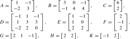
Carry out the matrix computations, or explain why they are impossible:
1. (i)
  BF;
2. (ii)
  AC;
3. (iii)
  CF;
4. (iv)
  BG;
5. (v)
  GD;
6. (vi)
  EK+KB.
5.
Suppose the first quarter’s menswear sales, in the department store of Sample Problem 5.30, are as shown. In each case, use matrices to calculate the profit for the quarter.
1. (i)
  
  Shirts
  Pants
  Jackets
  January
  150
  50
  20
  February
  130
  40
  40
  March
  140
  50
  15
2. (ii)
  
  Shirts
  Pants
  Jackets
  January
  60
  30
  12
  February
  15
  20
  10
  March
  35
  20
  25
6.
In each case, find the products AB and BA. Do the two matrices commute?
1. (i)
  $A = \left[\begin{array}{c@{\quad}c}0 & 1 \\2 & 3\end{array}\right],\qquad B = \left[\begin{array}{c@{\quad}c}1 & 2 \\-1 & 1\end{array}\right]$;
2. (ii)
  $A = \left[\begin{array}{c@{\quad}c}2 & 0 \\1 & -1\end{array}\right],\qquad B = \left[\begin{array}{c@{\quad}c}-2 & 4 \\3 & 2\end{array}\right]$;
3. (iii)
  $A = \left[\begin{array}{c@{\quad}c}3 & 1 \\-1 & 3\end{array}\right],\qquad B = \left[\begin{array}{c@{\quad}c}1 & 3 \\-3 & 1\end{array}\right]$.
7.
The matrix A is given. Find A ² and A ³.
1. (i)
  $\left[\begin{array}{c@{\quad}c}1 & 1 \\-1 & 1\end{array}\right]$;
2. (ii)
  $\left[\begin{array}{c@{\quad}c}-1 & -1 \\-1 & -1\end{array}\right]$;
3. (iii)
  $\left[\begin{array}{c@{\quad}c@{\quad}c}2 & 0 &3 \\0 & 3 &-1 \\-1 & -1 & 1\end{array}\right]$;
4. (iv)
  $\left[\begin{array}{c@{\quad}c@{\quad}c}3 &0 & -1 \\1 & 1 & 1 \\2 & 0 & -1\end{array}\right]$.
8.
Consider the matrix
$$A = \left[\begin{array}{c@{\quad}c}1 & 1 \\ -1 & 2\end{array}\right].$$
1. (i)
  Find A ² and A ³.
2. (ii)
  Evaluate A ³+A ²−3A.
3. (iii)
  Show that A ²−3A+3I=O.

Exercises 5.6 B

1.
Carry out the following vector calculations:
1. (i)
  (2,3)⋅(1,−1);
2. (ii)
  (1,3)⋅(2,−1);
3. (iii)
  (2,1,−1)⋅(3,0,1);
4. (iv)
  (1,1,−1)⋅(2,0,3);
5. (v)
  (4,2,1)⋅(1,2,4);
6. (vi)
  (2,2,−1)⋅(2,−2,−3);
7. (vii)
  (0,1,0,1)⋅(3,−1,2,2);
8. (viii)
  (0,2,1,1)⋅(3,4,2,1);
9. (ix)
  (3,−1,3,2)⋅(−1,−1,2,1);
10. (x)
  (1,−2,5,2)⋅(2,2,3,1).
2.
A is a 2×4 matrix; B is 2×4; C is 1×3; D is 4×2; E is 3×4; F is 4×3; G is 4×4. Say whether the indicated matrix exists. If it does exist, what is its shape?
1. (i)
  A+B;
2. (ii)
  CE;
3. (iii)
  D(A+B);
4. (iv)
  F ^T;
5. (v)
  2FC;
6. (vi)
  AD+DA;
7. (vii)
  GG;
8. (viii)
  DA+3G;
9. (ix)
  CFE.
3.
A is a 2×4 matrix; B is 3×4; C is 1×3; D is 4×2; E is 3×4; F is 4×2; G is 4×4. Say whether the indicated matrix exists. If it does exist, what is its shape?
1. (i)
  A+F;
2. (ii)
  AF;
3. (iii)
  A+F ^T;
4. (iv)
  AF ^T;
5. (v)
  FC;
6. (vi)
  ADA;
7. (vii)
  (B+E)F;
8. (viii)
  AGF;
9. (ix)
  AGE.
4.
Carry out the following matrix computations:
1. (i)
  $$\left[\begin{array}{c@{\quad}c} 3 & -1 \\2 & 0\end{array}\right] \left[\begin{array}{c@{\quad}c}4 & -2 \\-3 & 1\end{array}\right];$$
2. (ii)
  $$\left[\begin{array}{c@{\quad}c} 3 & -1 \\2 & 0\end{array}\right]^T \left[\begin{array}{c@{\quad}c}4 & -2 \\-3 & 1\end{array}\right];$$
3. (iii)
  $$\left[\begin{array}{c@{\quad}c}3 & -4 \\3 & 0\end{array}\right] \left[\begin{array}{c@{\quad}c}6 & -2 \\-7 & 4\end{array}\right];$$
4. (iv)
  $$\left[\begin{array}{c@{\quad}c}2 & -1 \\1 & -1 \\-1 & 1\end{array}\right]\left[\begin{array}{c@{\quad}c@{\quad}c}2 & 0 & 1 \\3 & -1 & 1\end{array}\right];$$
5. (v)
  $$\left[\begin{array}{c@{\quad}c}1 & -1 \\1 & 2 \\-3 & 1\end{array}\right]\left[\begin{array}{c@{\quad}c@{\quad}c} 1 & 0 & 2 \\3 & 1 & 1\end{array}\right];$$
6. (vi)
  $$\left[\begin{array}{c@{\quad}c@{\quad}c}2 & 1 & -1 \\1 & -1 & 2 \\-1 & 2 & -1\end{array}\right]\left[\begin{array}{c@{\quad}c@{\quad}c} 1 & 0 & 2 \\1 & 1 & -1\end{array}\right]^T.$$
5.
In this exercise,
Carry out the matrix computations, or explain why they are impossible:
1. (i)
  BD;
2. (ii)
  EF;
3. (iii)
  D−EB;
4. (iv)
  KB;
5. (v)
  CE ^T;
6. (vi)
  BK ^T+AH ^T.
6.
A manufacturer sells three products: hard drives, zip drives and flash drives. The number that were sold in its US and Canada markets in April were given by the following matrix M.

Hard
Zip
Flash
USA
5000
1000
9000
Canada
1000
300
2000
Prices, in dollars, for the three products are
$$S = \left[\begin{array}{c}150 \\100 \\50\end{array}\right],$$
respectively, while the manufacturing costs are
$$T = \left[\begin{array}{c}100 \\70 \\30\end{array}\right].$$
1. (i)
  Calculate the matrix quantities MS, MT, and M(S−T).
2. (ii)
  Interpret the matrix quantities MS, MT, and M(S−T).
3. (iii)
  What was the total profit in April?
7.
An automobile dealership sells three models of new cars. The profit from a sale is $1200 per economy sedan, $2000 per family sedan, and $2200 per coupe. Write down a matrix product that gives the profit for the first three months of the year, given that the dealership sells e _i economy sedans, f _i family sedans, and c _i coupes in month i. Use the product to calculate the profit in the following cases:
1. (i)
  
  Economy
  Family
  Coupe
  January
  15
  8
  2
  February
  11
  14
  4
  March
  14
  6
  3
2. (ii)
  
  Economy
  Family
  Coupe
  January
  25
  8
  2
  February
  10
  8
  5
  March
  5
  11
  7
8.
In each case, find the products AB and BA. Do the two matrices commute?
1. (i)
  $$A = \left[\begin{array}{c@{\quad}c}1 &-1 \\1 &1\end{array}\right],\qquad B = \left[\begin{array}{c@{\quad}c}2 & 1 \\-1 & 2\end{array}\right];$$
2. (ii)
  $$A = \left[\begin{array}{c@{\quad}c}1 & 2 \\3 &4\end{array}\right],\qquad B = \left[\begin{array}{c@{\quad}c}4 & 3 \\2 & 1\end{array}\right];$$
3. (iii)
  $$A = \left[\begin{array}{c@{\quad}c}1 &1 \\-2 &1\end{array}\right],\qquad B = \left[\begin{array}{c@{\quad}c}4 & -5 \\ 10 & 4\end{array}\right];$$
4. (iv)
  $$A = \left[\begin{array}{c@{\quad}c}1 & 1 \\3 & -2\end{array}\right],\qquad B = \left[\begin{array}{c@{\quad}c}2 & -3 \\1 & 1\end{array}\right];$$
5. (v)
  $$A = \left[\begin{array}{c@{\quad}c@{\quad}c}2 & 2 & 2 \\0 & 1 & 0 \\ 2 & 1 & 2\end{array}\right],\qquad B = \left[\begin{array}{c@{\quad}c@{\quad}c}2 & 2 & 2 \\0 & -1 & 0 \\2 & 3 & 2\end{array}\right];$$
6. (vi)
  $$A = \left[\begin{array}{c@{\quad}c@{\quad}c}3 & 1 &-2 \\1 & 2 &-1 \\-1 & -1 & 3\end{array}\right],\qquad B = \left[\begin{array}{c@{\quad}c@{\quad}c}2 & 0 & 1 \\-1 & 3 & 0 \\0 & 1 & 2\end{array}\right].$$
9.
The matrix A is given. Find A ² and A ³.
1. (i)
  $\left[\begin{array}{c@{\quad}c}2 & -1 \\-1 & 0\end{array}\right]$;
2. (ii)
  $\left[\begin{array}{c@{\quad}c}1 & 3 \\-1 & 1\end{array}\right]$;
3. (iii)
  $\left[\begin{array}{c@{\quad}c} 1 & -1 \\ -2 & 1\end{array}\right]$;
4. (iv)
  $\left[\begin{array}{c@{\quad}c} 2 & 1 \\3 & 2\end{array}\right]$;
5. (v)
  $\left[\begin{array}{c@{\quad}c@{\quad}c} 1 &0 & 1 \\ 1 & 1 & 0 \\ 0 & 1 & 1\end{array}\right]$;
6. (vi)
  $\left[\begin{array}{c@{\quad}c@{\quad}c}1 &-1 & 1 \\ -1 & 1 & 1 \\1 & 1 & -1\end{array}\right]$;
7. (vii)
  $\left[\begin{array}{c@{\quad}c@{\quad}c}1 &2 & 1 \\0 & -1 & 1 \\0 & 0 & -2\end{array}\right]$;
8. (viii)
  $\left[\begin{array}{c@{\quad}c@{\quad}c}1 &4& 0 \\0 & 1 & 3 \\1 & 0 & -1\end{array}\right]$.
10.
Consider the matrix
$$A = \left[\begin{array}{c@{\quad}c}1 & 3 \\5 & 3\end{array}\right].$$
1. (i)
  Find A ² and A ³.
2. (ii)
  Evaluate A ³−2A−I.
3. (iii)
  Show that A ²−4A−12I=O.
11.
A and B are any two matrices such that AB exists. Prove that B ^T A ^T exists, and that
$$B^TA^T = (AB)^T.$$

5.7 Inverses

If the matrices A and B satisfy AB=BA=I, we say that B is an inverse of A.

Which matrices have inverses? In the real numbers, everything but 0 has an inverse. In the integers, only 1 and −1 have integer inverses, but we know that we can obtain inverses of other non-zero integers by going to the rational numbers. The situation is more complicated for matrices.

Suppose A is an r×c matrix. Then AB has r rows and BA has c columns. If the two are to be equal, then AB is an r×c matrix; and if this is to equal an identity matrix, it must be square. So r=c, and A is also a square matrix. Only a square matrix can have an inverse.

Moreover, there are non-zero square matrices without inverses. Even if we restrict our attention to the 2×2 case, there are examples.

Sample Problem 5.32

Show that the matrix

$$A = \left[\begin{array}{c@{\quad}c}2 & 1 \\2 & 1\end{array}\right]$$

has no inverse.

Solution

Suppose A has inverse

$$B = \left[\begin{array}{c@{\quad}c}x & y \\z & t\end{array}\right] .$$

Then AB=I, so

$$\left[\begin{array}{c@{\quad}c}2 & 1 \\2 & 1\end{array}\right] \left[\begin{array}{c@{\quad}c}x & y \\z & t\end{array}\right] = \left[\begin{array}{c@{\quad}c}2x+z & 2y+t \\2x+z & 2y+t\end{array}\right] = \left[\begin{array}{c@{\quad}c}1 & 0 \\0 & 1\end{array}\right] .$$

The (1,1) entries of the two matrices must be equal, so 2x+z=1; but the (2,1) entries must also be equal, so 2x+z=0. This is impossible.

Your Turn

Show that the matrices

$$C = \left[\begin{array}{c@{\quad}c}1 & 0 \\0 & 0\end{array}\right]\quad \mbox{and}\quad D = \left[\begin{array}{c@{\quad}c}0 & 1 \\0 & 0\end{array}\right]$$

have no inverses.

A matrix that has an inverse will be called invertible or non-singular; a square matrix without an inverse is called singular.

We used the phrase “an inverse” above. However, we shall show that, if a matrix has an inverse, it is unique. We normally write it as A ⁻¹, just as with numbers, but the notation $\frac{1}{A}$ is never used for matrices.

Theorem 19

If matrices A,B,C satisfy AB=BA=I and AC=CA=I, then B=C.

Proof

Suppose A,B and C satisfy the given equations. Then

$$C = CI = C(AB) = (CA)B = IB = B$$

so B and C are equal. □

In fact, it can be shown that either of the conditions AB=I or BA=I is enough to determine that B is the inverse of A. However, this requires more algebra than we shall cover in this book.

Sample Problem 5.33

Suppose

$$A = \left[\begin{array}{c@{\quad}c}3 & 2 \\4 & 3\end{array}\right],\qquad B = \left[\begin{array}{c@{\quad}c}2 & 1 \\1 & 1\end{array}\right].$$

What is the inverse of A if it exists?

Solution

Suppose the inverse is

$$C = \left[\begin{array}{c@{\quad}c}x & z \\y & t\end{array}\right] .$$

Then AC=I means

$$\left[\begin{array}{c@{\quad}c}3 & 2 \\4 & 3\end{array}\right] \left[\begin{array}{c@{\quad}c}x & z \\y & t\end{array}\right] = \left[\begin{array}{c@{\quad}c}1 & 0 \\0 & 1\end{array}\right]$$

which is equivalent to the four equations

$$\begin{array}{rcl@{\qquad}rcl}3x + 2y & = & 1, & 3z + 2t & = & 0, \\[3pt]4x + 3y & = & 0, & 4z + 3t & = & 1.\end{array}$$

The left-hand pair of equations is easily solved to give x=3 and y=−4, while the right-hand pair give z=−2 and t=3. So the inverse exists, and is

$$A^{-1} = C = \left[\begin{array}{c@{\quad}c}3 & -2 \\-4 & 3\end{array}\right] .$$

Your Turn

What is the inverse of B if it exists?

The above procedure can be used to invert square matrices of any order; if there is no inverse, then the equations will have no solution. We shall now show how to reduce the number of computations required.

5.7.1 Calculating the Inverse

The inverse of a square matrix can be calculated by the algorithm used for solving equations. Suppose A is an n×n matrix with inverse B. Write $\textbf{\textit{b}}_{1}, \textbf{\textit{b}}_{2},\ldots, \textbf{\textit{b}}_{n}$ for the columns of B, and write $\textbf{\textit{u}}_{1}, \textbf{\textit{u}}_{2}, \ldots, \textbf{\textit{u}}_{n}$ for the columns of the identity matrix of order n. Consider the equation AB=I. Column j of the left-hand side is $A\textbf{\textit{b}}_{j}$. So the equation is equivalent to the set of n systems

$$A \textbf{\textit{b}}_1 = \textbf{\textit{u}}_1,\qquad A \textbf{\textit{b}}_2 = \textbf{\textit{u}}_2,\qquad \ldots,\qquad A \textbf{\textit{b}}_n = \textbf{\textit{u}}_n.$$

If all these systems have solutions, then the inverse is formed by putting the solution vectors next to each other in order. If any system has no solution, there is no inverse.

To solve $A \textbf{\textit{b}}_{j} = \textbf{\textit{u}}_{j}$, we reduce the augmented matrix $[ A \mid \textbf{\textit{u}}_{j} ]$ to reduced row echelon form. The same steps will produce this result, no matter what vector is on the right-hand side. It follows that we can carry out the reduction simultaneously for all n systems of equations. So we have the following technique for inverting an n×n matrix A.

Row reduce the matrix [A∣I _n]. If the resulting matrix has form [I _n∣B] then A is invertible, and B is A ⁻¹ . Otherwise, A is singular.

It follows from this that if a matrix has a row with every entry zero, it must be singular. This is also true if the matrix has a column with every entry zero. For example, if A has every entry of its first column zero, then BA has every element zero in its first column for any choice of B, so the equation A ⁻¹ A=I cannot possibly be true—it must fail in the (1,1) position.

Sample Problem 5.34

For the following matrices, find the inverse or show that the matrix is singular:

$$A = \left[\begin{array}{c@{\quad}c@{\quad}c}1& 2& -1 \\0& -2& 1 \\1&1&-1\end{array}\right],\qquad B = \left[\begin{array}{c@{\quad}c@{\quad}c}2& 3& 2 \\3& -1& 2 \\1&7& 2\end{array}\right].$$

Solution

For A, we have

So A has inverse

$$\left[\begin{array}{c@{\quad}c@{\quad}c}1 & 1 & 0 \\1 & 0 & -1 \\2 & 1 & -2\end{array}\right].$$

For B, we get

and the zero row on the left tells us that B is singular.

Your Turn

In the above calculations, identify the steps that have been taken at each stage. (For example, for A, the first step was R3←R3−R1.)

This method can be used to get a general solution for the inverse of a 2×2 matrix.

Theorem 20

The matrix

$$A = \left[\begin{array}{c@{\quad}c}a & b \\c & d\end{array}\right]$$

is singular if ad−bc=0. Otherwise it is invertible, with inverse

$$\frac{1}{(ad-bc)}\left[\begin{array}{c@{\quad}c} d & -b \\-c & a\end{array}\right]. $$

(5.3)

Proof

If a=c=0, then ad−bc=0. Moreover A has a zero column, so as we saw it has no inverse. So we need only consider cases where a, c, or both are non-zero.

First, suppose a and c are both non-zero. The inverse procedure is

If ad−bc=0, then we are finished and there is no inverse. Otherwise, notice that

$${ 1+\frac{bc}{ad-bc} =\frac{ad-bc+bc}{ad-bc} =\frac{ad}{ad-bc}},$$

so we have

as required.

If a≠0 and c=0 the calculations are simpler. We obtain the inverse

$$\left[\begin{array}{c@{\quad}c}\frac{1}{a}&-\frac{b}{ad} \\[5pt]0 &\frac{1}{d}\end{array}\right]$$

and this is the form taken by (5.3) when c=0.

The case where a=0,c≠0 is similar to the latter case. □

5.7.2 The Determinant

The number ad−bc is called the determinant of the matrix A, written det(A). Determinants may be defined for square matrices of any order, and it is a general theorem that a matrix is invertible if and only if its determinant is non-zero. However, we need only consider the 2×2 case.

Sample Problem 5.35

Find the determinants of the following matrices and use them to find their inverses, if possible:

$$A = \left[\begin{array}{c@{\quad}c}3& 1 \\2& 2\end{array}\right],\qquad B = \left[\begin{array}{c@{\quad}c}2& -2 \\-1& 1\end{array}\right].$$

Solution

det(A)=3⋅2−1⋅2=4, so

$$A^{-1} = \frac{1}{4} \left[\begin{array}{c@{\quad}c}2& -1 \\-2& 3\end{array}\right]= \left[\begin{array}{c@{\quad}c}\frac{1}{2}& -\frac{1}{4} \\[4pt]-\frac{1}{2}& \frac{3}{4}\end{array}\right].$$

det(B)=2⋅1−(−2)⋅(−1)=0, so B has no inverse.

Your Turn

Repeat for

$$C = \left[\begin{array}{c@{\quad}c}1& 1 \\3& 4\end{array}\right],\qquad D = \left[\begin{array}{c@{\quad}c}2& 4 \\1& 2\end{array}\right].$$

Exercises 5.7 A

1.
Show that the given matrices are inverses:
1. (i)
  $\left[\begin{array}[c]{c@{\quad}c}{\textstyle\frac{3}{2}} & -1 \\0 & 1\end{array}\right]\quad \mbox{and}\quad \left[\begin{array}{c@{\quad}c}{\textstyle\frac{2}{3}} & {\textstyle\frac{2}{3}} \\0 & 1\end{array}\right]$;
2. (ii)
  $\left[\begin{array}{c@{\quad}c}2 & -3 \\-1 & 2\end{array}\right]\quad \mbox{and}\quad \left[\begin{array}{c@{\quad}c}2 & 3 \\1 & 2\end{array}\right]$.
2.
Find matrices A and B such that
1. (i)
  $A\left[\begin{array}{c@{\quad}c}3 & 2 \\2 & 1\end{array}\right] = \left[\begin{array}{c@{\quad}c}1 & 3 \\2 & -1\end{array}\right]$;
2. (ii)
  $B\left[\begin{array}{c@{\quad}c}2 & 1 \\3 & 2\end{array}\right] = \left[\begin{array}{c@{\quad}c}1 & -1 \\1 & 4\end{array}\right]$.
3.
Use row reduction either to find the inverse of the given matrix or to show that the matrix is singular:
1. (i)
  $\left[\begin{array}{c@{\quad}c}2 &-2 \\4 & 0\end{array}\right]$;
2. (ii)
  $\left[\begin{array}{c@{\quad}c}3 &7 \\2 & 5\end{array}\right]$;
3. (iii)
  $\left[\begin{array}{c@{\quad}c}4 &2 \\2 & 1\end{array}\right]$;
4. (iv)
  $\left[\begin{array}{c@{\quad}c@{\quad}c}0 & 0 & 1 \\0 & 1 & 0 \\1 & 0 & 1\end{array}\right]$;
5. (v)
  $\left[\begin{array}{c@{\quad}c@{\quad}c}2 & 3 & 2 \\1 & 2 & 2 \\3 & 1 & 3\end{array}\right]$;
6. (vi)
  $\left[\begin{array}{c@{\quad}c@{\quad}c}0 & 1 & 1 \\5 & 1 & -2 \\2 & -3 & -3\end{array}\right]$;
7. (vii)
  $\left[\begin{array}{c@{\quad}c@{\quad}c}1 & 3 & 3 \\1 & 4 & 3 \\1 & 3 & 4\end{array}\right]$;
8. (viii)
  $\left[\begin{array}{c@{\quad}c@{\quad}c}1 & 1& -1 \\-2 & -1 & 7 \\3 & 2 &-8\end{array}\right]$.
4.
Find the determinant of the matrix, and use it to invert the matrix or show that it is singular:
1. (i)
  $\left[\begin{array}{c@{\quad}c}7 & 4 \\2 & 3\end{array}\right]$;
2. (ii)
  $\left[\begin{array}{c@{\quad}c}-2 & 2 \\2 & 3\end{array}\right]$;
3. (iii)
  $\left[\begin{array}{c@{\quad}c}4 & 2 \\8 & 4\end{array}\right]$;
4. (iv)
  $\left[\begin{array}{c@{\quad}c}3 & 2 \\1 & 1\end{array}\right]$.

Exercises 5.7 B

1.
Show that the given matrices are inverses:
1. (i)
  $\left[\begin{array}{c@{\quad}c}2 & 5 \\1 & 3\end{array}\right]\quad \mbox{and}\quad \left[\begin{array}{c@{\quad}c}3 & -5 \\-1 & 2\end{array}\right]$;
2. (ii)
  $\left[\begin{array}{c@{\quad}c}{\textstyle{\frac{1}{2}} }& -1 \\1 & -1\end{array}\right]\quad \mbox{and}\quad \left[\begin{array}{c@{\quad}c}-2 & 2 \\-2 & 1\end{array}\right]$.
2.
Find matrices A, B, and C such that
1. (i)
  $A\left[\begin{array}{c@{\quad}c} 1 & -1 \\3 & 1\end{array}\right] = \left[\begin{array}{c@{\quad}c}5 & -1 \\2 & 2\end{array}\right]$;
2. (ii)
  $B\left[\begin{array}{c@{\quad}c} -1 & 2 \\ -2 & 2\end{array}\right] = \left[\begin{array}{c@{\quad}c}1 & 2 \\ -3 & 2\end{array}\right]$;
3. (iii)
  $\left[\begin{array}{c@{\quad}c}3 & 1 \\ 1 & -2\end{array}\right] C = \left[\begin{array}{c@{\quad}c}7 & 3 \\0 & 1\end{array}\right]$.
3.
Use row reduction either to find the inverse of the given matrix or to show that the matrix is singular:
1. (i)
  $\left[\begin{array}{c@{\quad}c}2 &-2 \\3 & -3\end{array}\right]$;
2. (ii)
  $\left[\begin{array}{c@{\quad}c}1 &1 \\1 & 0.5\end{array}\right]$;
3. (iii)
  $\left[\begin{array}{c@{\quad}c}3 &1 \\-4 & -2\end{array}\right]$;
4. (iv)
  $\left[\begin{array}{c@{\quad}c@{\quad}c}0 & 1 & 0 \\0 & 0 & 1 \\1 & 0 & 0\end{array}\right]$;
5. (v)
  $\left[\begin{array}{c@{\quad}c} 4 & 3 \\ 1 & 1\end{array}\right]$;
6. (vi)
  $\left[\begin{array}{c@{\quad}c}3 & 2 \\ 2 & 1\end{array}\right]$;
7. (vii)
  $\left[\begin{array}{c@{\quad}c}3 & -1 \\ -6 & 2\end{array}\right]$;
8. (viii)
  $\left[\begin{array}{c@{\quad}c}2 & 3 \\2 & 4\end{array}\right]$;
9. (ix)
  $\left[\begin{array}{c@{\quad}c@{\quad}c}9 & 8 & 7 \\6 & 5 & 4 \\3 & 2 & 1\end{array}\right]$;
10. (x)
  $\left[\begin{array}{c@{\quad}c@{\quad}c}1 & -2 & 3 \\3 & 5 & 1 \\6 & 4 & 2\end{array}\right]$;
11. (xi)
  $\left[\begin{array}{c@{\quad}c@{\quad}c}2 & 3 & -1 \\4 & 2 & 3 \\2 & 7 &-6\end{array}\right]$;
12. (xii)
  $\left[\begin{array}{c@{\quad}c@{\quad}c}1 & 0 & 2 \\2 & -1 & 3 \\4 & 1 & 8\end{array}\right]$;
13. (xiii)
  $\left[\begin{array}{c@{\quad}c@{\quad}c}1 & 2 & 3 \\2 & 5 & 1 \\3 & 7 & 4\end{array}\right]$;
14. (xiv)
  $\left[\begin{array}{c@{\quad}c@{\quad}c}1 & 2 & 3 \\2 & 5 & 5 \\3 & 8 & 8\end{array}\right]$;
15. (xv)
  $\left[\begin{array}{c@{\quad}c@{\quad}c}3 & 2 & 2 \\4 & 2 & 3 \\5 & 4 & 3\end{array}\right]$;
16. (xvi)
  $\left[\begin{array}{c@{\quad}c@{\quad}c}1 & 2 & 1 \\ -3 & -5 & -3 \\1 & 3 & 2\end{array}\right]$;
17. (xvii)
  $\left[\begin{array}{c@{\quad}c@{\quad}c}1 & 1 & 1 \\ 3 & 1 & -1 \\1 & 1 & 2\end{array}\right]$;
18. (xviii)
  $\left[\begin{array}{c@{\quad}c@{\quad}c}1 & 2 & -2 \\ 3 & 2 & 2 \\3 & 1 & 4\end{array}\right]$;
19. (xix)
  $\left[\begin{array}{c@{\quad}c@{\quad}c}1 & 1 & 1 \\0 & 1 & 1 \\2 & 2 & 3\end{array}\right]$;
20. (xx)
  $\left[\begin{array}{c@{\quad}c@{\quad}c}5 & 2& 1 \\ 4 & 2 & -1 \\3 & 1 & 3\end{array}\right]$.
4.
Find the determinant of the matrix, and use it to invert the matrix or show that it is singular:
1. (i)
  $\left[\begin{array}{c@{\quad}c}6 & 4 \\3 & 2\end{array}\right]$;
2. (ii)
  $\left[\begin{array}{c@{\quad}c}3 & 5 \\1 & 4\end{array}\right]$;
3. (iii)
  $\left[\begin{array}{c@{\quad}c}3 & 2 \\-1 & 1\end{array}\right]$;
4. (iv)
  $\left[\begin{array}{c@{\quad}c}6 & 4 \\7 & 5\end{array}\right]$;
5. (v)
  $\left[\begin{array}{c@{\quad}c}-1 & -3 \\1 & 2\end{array}\right]$;
6. (vi)
  $\left[\begin{array}{c@{\quad}c}2 & 5 \\1 & 4\end{array}\right]$;
7. (vii)
  $\left[\begin{array}{c@{\quad}c}3 & 6 \\-2 & -4\end{array}\right]$;
8. (viii)
  $\left[\begin{array}{c@{\quad}c}3 & -4 \\2 & -3\end{array}\right]$;
9. (ix)
  $\left[\begin{array}{c@{\quad}c}7 & 3 \\5 & 2\end{array}\right]$;
10. (x)
  $\left[\begin{array}{c@{\quad}c}6 & -2 \\-11 & 4\end{array}\right]$.

5.8 More About Inverses

5.8.1 Some Properties of Inverses

As we said, the usual notation for the inverse of A (if it exists) is A ⁻¹. If we define A ⁰=I whenever A is square, then powers of matrices satisfy the usual index laws

$$A^m A^n = A^{m+n},\qquad \bigl(A^m\bigr)^n = A^{mn}$$

for all non-negative integers m and n, and for negative values also provided that A ⁻¹ exists. If x and y are non-zero reals, then (xy)⁻¹=x ⁻¹ y ⁻¹. The fact that matrices do not necessarily commute means that we have to be a little more careful, and prove the following small theorem.

Theorem 21

If A and B are invertible matrices of the same order, then AB is invertible, and

$$(AB)^{-1} =B^{-1}A^{-1}.$$

Proof

We need to show that both (B ⁻¹ A ⁻¹)(AB) and (AB)(B ⁻¹ A ⁻¹) equal the identity. But (B ⁻¹ A ⁻¹)(AB)=B ⁻¹(A ⁻¹ A)B=B ⁻¹ IB=B ⁻¹ B=I=AA ⁻¹=AIA ⁻¹=A(BB ⁻¹)A ⁻¹=(AB)(B ⁻¹ A ⁻¹). □

There are two cancellation laws for matrix multiplication. If A is an invertible r×r matrix and B and C are r×s matrices such that AB=AC, then

so B=C. Similarly, if A is an invertible s×s matrix and B and C are r×s matrices such that BA=CA, then B=C.

The requirement that A be invertible is necessary. We can find matrices A,B, and C such that AB and AC are the same size, A is non-zero and AB=AC, but B and C are different. One very easy example is

$$\left[\begin{array}{c@{\quad}c}1 & 0 \\0 & 0\end{array}\right]\left[\begin{array}{c@{\quad}c}1 & -1 \\2 & 3\end{array}\right]= \left[\begin{array}{c@{\quad}c}1 & 0 \\0 & 0\end{array}\right]\left[\begin{array}{c@{\quad}c}1 & -1 \\1 & 4\end{array}\right].$$

Some other examples are given in the exercises.

Moreover, we can only cancel on one side of an equation; we cannot mix the two sides. Even if A is invertible it is possible that AB=CA but B≠C (see the exercises for examples of this, also).

5.8.2 Linear Systems and Inverses

Consider the system of equations $A \textbf{\textit{x}}= \textbf{\textit{b}}$, where A is an invertible matrix. Multiplying by A ⁻¹, $\textbf{\textit{x}}= A^{-1}A \textbf{\textit{x}}= A^{-1} \textbf{\textit{b}}$, so the equations have the unique solution $A^{-1} \textbf{\textit{b}}$. This could be used to solve the equations. This technique is not usually helpful in practical situations because the process of finding the inverse takes at least as long as solving the equations, but it is useful when there are several sets of equations with the same left-hand sides, or when the inverse is already known. It is also important in theoretical studies.

Sample Problem 5.36

Solve the systems:

$$\begin{array}{rcl@{\qquad}rcl}x + 2y - z & = & 3, & x + 2y - z & =& -1, \\[3pt]- 2y + z & = & 1, & - 2y + z & = & -2, \\ [3pt]x + y - z & = & 0; & x + y - z & = & 2.\end{array}$$

Solution

We saw in Sample Problem 5.34 that the matrix of coefficients has inverse

$$\left[\begin{array}{c@{\quad}c@{\quad}c}1 & 1 & 0 \\1 & 0 & -1 \\2 & 1 & -2\end{array}\right].$$

Now

$$\left[\begin{array}{c@{\quad}c@{\quad}c}1 & 1 & 0 \\1 & 0 & -1 \\2 & 1 & -2\end{array}\right] \left[\begin{array}{r}3 \\1 \\0\end{array}\right]= \left[\begin{array}{r}4 \\3 \\7\end{array}\right],$$

so the first system has solution x=4,y=3,z=7.

$$\left[\begin{array}{c@{\quad}c@{\quad}c}1 & 1 & 0 \\1 & 0 & -1 \\2 & 1 & -2\end{array}\right] \left[\begin{array}{r}-1 \\-2 \\2\end{array}\right]= \left[\begin{array}{r}-3 \\-3 \\-8\end{array}\right],$$

and the second has solution x=−3,y=−3,z=−8.

Your Turn

Solve the systems:

$$\begin{array}{rcl@{\qquad}rcl}x + 2y - z & = & 2, & x + 2y - z & = & 4, \\[3pt]- 2y + z & = & 2, & - 2y + z & = & -1, \\[3pt]x + y - z & = & 1; & x + y - z & = & 3.\end{array}$$

5.8.3 The Leontief Input–Output Model

Matrices have important applications in economics. One important example is the input–output model developed by Wassily Leontief in the 1950s. (He was awarded the Nobel Prize in economics for this work.)

We explain Leontief’s method using a very much oversimplified example. We shall describe a company that has no outside needs other than its own products—no outside costs, etc. This is unrealistic, but illustrates the main principles.

Suppose a company produces three petroleum products—gasoline, heating oil, and lubricating oil. During production of gasoline, a certain amount of each product is required, and naturally the company uses its own products. Suppose that, in order to produce a barrel of gasoline, it is necessary to use 0.2 barrels of gasoline, 0.1 barrels of heating oil, and 0.2 barrels of lubricating oil. Similarly, producing a barrel of heating oil uses 0.2 barrels of gasoline, 0.3 barrels of heating oil, and 0.1 barrels of lubricating oil, and a barrel of lubricating oil requires 0.1 barrels of gasoline, 0.2 barrels of heating oil, and 0.2 barrels of lubricating oil. This information can be summarized in the following matrix, called the technology matrix, or input–output matrix, of the system.

$$\addtolength{\arraycolsep}{2pt}T =\ \begin{array}{@{}llll@{}}\hline & \mathrm{Gas} & \mathrm{Heat} & \mathrm{Lub} \\\hline \mathrm{Gas} & 0.2 & 0.2 & 0.1 \\\mathrm{Heat} & 0.1 & 0.3 & 0.2 \\\mathrm{Lub} & 0.2 & 0.1 & 0.2 \\\hline \end{array}$$

Each column represents the demands of the system in producing one product. For example, in the “heating oil” column, the entry in the “gasoline” row says how much gasoline is needed to produce one barrel of heating oil.

Suppose the company produces 90 million barrels of gasoline, 60 million barrels of heating oil, and 70 million barrels of lubricating oil each year. Much of this product is consumed in production. To find out how much, we perform a matrix multiplication. First, we construct a column vector called the production matrix or total output matrix,

$$\addtolength{\arraycolsep}{2pt}P =\ \begin{array}{@{}ll@{}}\hline \mathrm{Gas} & 90 \\\mathrm{Heat} & 60 \\\mathrm{Lub} & 70 \\\hline \end{array}$$

Then the internal demand is

$$D_0 = TP =\left[\begin{array}{c@{\quad}c@{\quad}c}0.2 & 0.2 & 0.1 \\0.1 & 0.3 & 0.2 \\0.2 & 0.1 & 0.2\end{array}\right]\left[\begin{array}{c}90 \\60 \\70\end{array}\right] =\left[\begin{array}{c}37 \\41 \\38\end{array}\right]\quad \begin{array}{l}\mathrm{Gas}, \\\mathrm{Heat}, \\\mathrm{Lub}.\end{array}$$

So 37 million barrels of gasoline, 41 million barrels of heating oil, and 38 million barrels of lubricating oil is consumed within the company. This is called the internal demand and D ₀ is the internal demand matrix.

We can now calculate how much of each product is available for outside users, how much the company can actually sell. This amount is

$$D = P - D_0 = \left[\begin{array}{c}90 \\60 \\70\end{array}\right] -\left[\begin{array}{c}37 \\41 \\38\end{array}\right]=\left[\begin{array}{c}53 \\19 \\32\end{array}\right]\quad \begin{array}{l}\mathrm{Gas} \\\mathrm{Heat} \\\mathrm{Lub}\end{array}$$

If the company is operating efficiently, this vector will show exactly how much is being bought by customers, so it is called the external demand matrix. The fundamental equation of input–output analysis is

$$ P = TP + D. $$

(5.4)

5.8.4 Using the Leontief Model

Usually the values in P are not given to us. The typical problem encountered by a company is, given the external demands by our customers and the needs of our processes, how much of each product should we produce?

Equation (5.4) can be rewritten as

$$P - TP = D,$$

or

$$(I - T) P = D.$$

If the matrix I−T has an inverse, then

$$P = (I - T)^{-1} D.$$

So we have the following result.

Theorem 22

If a company is to meet its external demands, then the total production P satisfies

$$P = (I - T)^{-1} D.$$

If the matrix I−T has no inverse, the company cannot meet its demands.

In our ongoing example, the matrix was

$$I-T =\left[\begin{array}{c@{\quad}c@{\quad}c}0.8 & -0.2 & -0.1 \\-0.1 & 0.7 & -0.2 \\-0.2 & -0.1 & 0.8\end{array}\right].$$

This matrix has inverse

$$(I-T)^{-1} =\frac{1}{393}\left[\begin{array}{c@{\quad}c@{\quad}c}540 & 170 & 110 \\120 & 620 & 170 \\150 & 120 & 540\end{array}\right].$$

Notice that the elements in (I−T)⁻¹ are quite small numbers. This will often happen. All entries in I−T will be less than 1, and they will usually be given in decimal form. In calculating the inverse, you will find it easier to invert $\frac {1}{10}(I-T)$ (or even $\frac{1}{100}(I-T)$), and multiply the resulting inverse by 10 (or 100).

Sample Problem 5.37

Suppose our oil company has an external demand of 50 million barrels of gasoline, 30 million barrels of heating oil, and 20 million barrels of lubricating oil. How much of each product should be produced?

Solution

So the company should produce 87277000 barrels of gasoline, 71247000 barrels of heating oil, and 55725000 barrels of lubricating oil.

Leontief’s original application was not to companies, but to the economies of countries. Rather than individual products, he dealt with whole sectors of the economy: the oil industry, the electric power industry, the electronics industry, and so on. He identified 81 sectors of the U.S. economy, and applied his analysis to it. Such an analysis, applied to a small country, can identify areas where the economy cannot meet its demands, and is used to suggest which commodities must be imported, which trade agreements should therefore be strengthened, and so on.

Sample Problem 5.38

A farming community produces two commodities, beef and vegetables. Beef production uses 0.3 pounds of beef and 0.1 pounds of vegetables, to feed animals and workers, for each pound produced. Vegetable production requires 0.2 pounds of beef and 0.4 pounds of vegetables. There is external demand for 24000 pounds of beef and 16000 pounds of vegetables. How much should be produced?

Solution

The technology matrix is

$$T = \left[\begin{array}{c@{\quad}c}0.3 & 0.2 \\0.1 & 0.4\end{array}\right]$$

and

$$(I-T) = \left[\begin{array}{c@{\quad}c}0.7 & -0.2 \\-0.1 & 0.6\end{array}\right]$$

which has determinant 0.42−0.02=0.4. So

$$(I-T)^{-1} = 2.5 \left[\begin{array}{c@{\quad}c}0.6 & 0.2 \\0.1 & 0.7\end{array}\right] = \left[\begin{array}{c@{\quad}c}1.5 & 0.5 \\0.25 & 1.75\end{array}\right],$$

so

$$P = \left[\begin{array}{c@{\quad}c}1.5 & 0.5 \\0.25 & 1.75\end{array}\right] \left[\begin{array}{c}24000 \\16000\end{array}\right] = \left[\begin{array}{c}44000 \\34000\end{array}\right].$$

So the required production is 44000 pounds of beef and 34000 pounds of vegetables.

Your Turn

An economy produces coal and steel. Each ton of steel requires 0.3 tons of steel and 0.5 tons of coal in its production. Each ton of coal requires 0.2 tons of steel and 0.5 tons of coal. In order to supply an outside demand for 25 tons of steel and 50 tons of coal, how much should be produced?

Exercises 5.8 A

1.
In each case show that AB=AC:
1. (i)
  $A = \left[\begin{array}{c@{\quad}c}1 & -1 \\2 & -2\end{array}\right], \qquad B = \left[\begin{array}{c@{\quad}c}2 & 1 \\1 & 4\end{array}\right],\qquad C = \left[\begin{array}{c@{\quad}c}4 & 0 \\3 & 3\end{array}\right]$;
2. (ii)
  $A = \left[\begin{array}{c@{\quad}c@{\quad}c}1 & 0 & 1 \\1 & 1 & 1 \\1 & 2 & 1\end{array}\right], \qquad B = \left[\begin{array}{c@{\quad}c@{\quad}c}1 & 1 & 2 \\1 & 1 & 0 \\1 & 2 & 2\end{array}\right], \qquad C = \left[\begin{array}{c@{\quad}c@{\quad}c}2 & 2 & 1 \\1 & 1 & 0 \\0 & 1 & 3\end{array}\right]$.
2.
Show that A ⁻¹ exists, but AB=CA, even though B≠C:
$$A = \left[\begin{array}{c@{\quad}c}-1 & 3 \\1 & -2\end{array}\right], \qquad B = \left[\begin{array}{c@{\quad}c}1 & 2 \\1 & 1\end{array}\right], \qquad C = \left[\begin{array}{c@{\quad}c}5 & 7 \\-2 & -3\end{array}\right].$$
3.
1. (i)
  Prove that the following matrices are inverses:
  $$\left[\begin{array}{c@{\quad}c}3& 2 \\1& 1\end{array}\right],\quad \left[\begin{array}{c@{\quad}c}1& -2 \\-1& 3\end{array}\right];$$
2. (ii)
  Use part (i) to solve the following systems:
  $$\begin{array}{l@{\quad}rcl@{\qquad}l@{\quad}rcl}\mbox{(a)} & 3x + 2y & = & 4, & \mbox{(b)} & x - 2y & = & -1, \\[4pt]& x + y & = & 1; & & -x + 3y & = & 2.\end{array}$$
4.
1. (i)
  Prove that the following matrices are inverses:
  $$\left[\begin{array}{c@{\quad}c@{\quad}c}3 & 5 & 7 \\1 & 2 & 3 \\2 & 3 & 5\end{array}\right],\quad \left[\begin{array}{c@{\quad}c@{\quad}c}1& -4& 1 \\1& 1& -2 \\ -1& 1& 1\end{array}\right];$$
2. (ii)
  Use part (i) to solve the following systems.
  $$\begin{array}{l@{\quad}rcl@{\qquad}l@{\quad}rcl}\mbox{(a)} & 3x + 5y + 7z & = & 1, & \mbox{(b)} & x - 4y + z & = & 2, \\[4pt]& x + 2y + 3z & = & 2, & & x + y - 2z & = & 1, \\[4pt]& 2x + 3y + 5z & = & 1; & & -x + y + z & = & -1.\end{array}$$
5.
In each case the technology matrix T and external demand matrix D for a two-sector economy are shown. What is the associated production matrix P?
1. (i)
  $T = \left[\begin{array}{c@{\quad}c}0.3& 0.6 \\0.4& 0.3\end{array}\right],\qquad D = \left[\begin{array}{r}30 \\20\end{array}\right]$;
2. (ii)
  $T = \left[\begin{array}{c@{\quad}c}0.2& 0.1 \\0.2& 0.6\end{array}\right], \qquad D = \left[\begin{array}{r}42 \\36\end{array}\right]$;
3. (iii)
  $T = \left[\begin{array}{c@{\quad}c}0.1& 0.1 \\0.2& 0.2\end{array}\right], \qquad D = \left[\begin{array}{r}20 \\30\end{array}\right]$;
4. (iv)
  $T = \left[\begin{array}{c@{\quad}c}0.4& 0.2 \\0.4& 0.2\end{array}\right],\qquad D = \left[\begin{array}{r}200 \\120\end{array}\right]$.
6.
An economy produces two products, X and Y. To produce each kilogram of X, one must use 500 grams of X and 250 grams of Y. To produce each kilogram of Y, one must use 100 grams of X and 250 grams of Y. In a certain week, the external demand is 84 tonnes of X and 98 tonnes of Y. What is the required production?

Exercises 5.8 B

1.
In each case show that AB=AC:
1. (i)
  $A = \left[\begin{array}{c@{\quad}c}2 & 1 \\4 & 2\end{array}\right],\qquad B = \left[\begin{array}{c@{\quad}c}0 & 1 \\3 & 7\end{array}\right], \qquad C = \left[\begin{array}{c@{\quad}c}1 & 4 \\1 & 1\end{array}\right]$;
2. (ii)
  $\begin{array}[t]{rcl}A &=& \left[\begin{array}{c@{\quad}c@{\quad}c}1 & 2 & 5 \\3 & -1 & 1 \\2 & 1 & 4\end{array}\right], \qquad B = \left[\begin{array}{c@{\quad}c@{\quad}c}1 & -2 & 2 \\-1 & 0 & 3 \\2 & 0 & 1\end{array}\right], \\[20pt]C &=& \left[\begin{array}{c@{\quad}c@{\quad}c}2 & -1 & 1 \\1 & 2 & 1 \\1 & -1 & 2\end{array}\right].\end{array}$
2.
Show that A ⁻¹ exists, but AB=CA, even though B≠C, when
$$A = \left[\begin{array}{c@{\quad}c}2 & -1 \\1 & 1\end{array}\right],\qquad B = \left[\begin{array}{c@{\quad}c}3 & 0 \\4 & 1\end{array}\right], \qquad C = \left[\begin{array}{c@{\quad}c}1 & 0 \\2 & 3\end{array}\right].$$
3.
Find a matrix A such that
$$\left[\begin{array}{c@{\quad}c} 0 & 1 \\ 1 & 0\end{array}\right] A \left[\begin{array}{c@{\quad}c} 1 & 1 \\ 0 & 1\end{array}\right] = \left[\begin{array}{c@{\quad}c} 2 & 1 \\ 3 & 2\end{array}\right].$$
4.
1. (i)
  Prove that the following matrices are inverses:
  $$\left[\begin{array}{c@{\quad}c@{\quad}c}1 & 2 & 3 \\1 & 1 & 1 \\1 & 1 & 2\end{array}\right],\quad \left[\begin{array}{c@{\quad}c@{\quad}c}-1& 1& 1 \\1& 1& -2 \\0& -1& 1\end{array}\right];$$
2. (ii)
  Use part (i) to solve the following systems:
  $$\begin{array}{l@{\quad}rcl@{\qquad}l@{\quad}rcl}\mbox{(a)} & x + 2y + 3z & = & 3, & \mbox{(b)} & -x + y + z & = & -1, \\[4pt]& x + y + z & = & 1, & & x + y - 2z & = & 0, \\[4pt]& x + y + 2z & = & 4; & & - y + z & = & 1.\end{array}$$
5.
1. (i)
  Prove that the following matrices are inverses:
  $$\left[\begin{array}{c@{\quad}c@{\quad}c}2& -2& 1 \\1& 0& 1 \\1& -3& 0\end{array}\right],\quad \left[\begin{array}{c@{\quad}c@{\quad}c}3& -3& -2 \\1& -1& -1 \\-3& 4& 2\end{array}\right];$$
2. (ii)
  Use part (i) to solve the following systems:
  $$\begin{array}{l@{\quad}rcl@{\qquad}l@{\quad}rcl}\mbox{(a)} & 2x - 2y + z & = & 3, & \mbox{(b)} & 3x - 3y - 2z & = & 2,\\[4pt]& x + z & = & 2, & & x - y - z & = & -1, \\[4pt]& x - 3y & = & 1; & &-3x + 4y + 2z & = & 2.\end{array}$$
6.
In each case the technology matrix T and external demand matrix D for a two-sector economy are shown. What is the associated production matrix P?
1. (i)
  $$T = \left[\begin{array}{c@{\quad}c}0.4& 0.2 \\0.3& 0.4\end{array}\right],\qquad D = \left[\begin{array}{c}30 \\45\end{array}\right];$$
2. (ii)
  $$T = \left[\begin{array}{c@{\quad}c}0.3& 0.3 \\0.4& 0.4\end{array}\right], \qquad D = \left[\begin{array}{c}42 \\36\end{array}\right];$$
3. (iii)
  $$T = \left[\begin{array}{c@{\quad}c}0.7& 0.2 \\0.2& 0.2\end{array}\right],\qquad D = \left[\begin{array}{c}40 \\88\end{array}\right];$$
4. (iv)
  $$T = \left[\begin{array}{c@{\quad}c}0.2& 0.2 \\0.3& 0.3\end{array}\right], \qquad D = \left[\begin{array}{c}70 \\80\end{array}\right];$$
5. (v)
  $$T = \left[\begin{array}{c@{\quad}c}0.6& 0.2 \\0.2& 0.4\end{array}\right],\qquad D = \left[\begin{array}{c}40 \\60\end{array}\right];$$
6. (vi)
  $$T = \left[\begin{array}{c@{\quad}c}0.4& 0.7 \\0.4& 0.2\end{array}\right], \qquad D = \left[\begin{array}{c}44 \\28\end{array}\right];$$
7. (vii)
  $$T = \left[\begin{array}{c@{\quad}c}0.25 & 0.1 \\0.25 & 0.2\end{array}\right], \qquad D = \left[\begin{array}{c}690 \\460\end{array}\right];$$
8. (viii)
  $$T = \left[\begin{array}{c@{\quad}c}0.9& 0.2 \\0.1& 0.6\end{array}\right],\qquad D = \left[\begin{array}{c}100 \\200\end{array}\right].$$
7.
In a three-sector economy the technology matrix T and external demand matrix D are
$$T = \left[\begin{array}{c@{\quad}c@{\quad}c}0.2& 0.2 & 0.4 \\0.2& 0.2 & 0.4 \\0.1& 0.6 & 0.2\end{array}\right], \qquad D = \left[\begin{array}{r}40 \\30 \\45\end{array}\right].$$
What is the associated production matrix P?
8.
An economy produces three products, A, B, and C. To produce a hundred pounds of A requires 30 pounds of A, 30 pounds of B, and 10 pounds of C. To produce 100 pounds of B requires 10 pounds of A and 50 pounds of B (no C is used). To produce 100 pounds of C requires 50 pounds of A, 10 pounds of B and 70 pounds of C. What is the required production in the following cases?
1. (i)
  In the first quarter of the year, there was external demand for 7000 pounds of A, 14000 pounds of B, and 21000 pounds of C.
2. (ii)
  In the second quarter, there was external demand for 14000 pounds of A, 7000 pounds of B, and 14000 pounds of C.
9.
Suppose M _x denotes the 2×2 matrix
$$\left[\begin{array}{c@{\quad}c}1 & x \\0 & 1\end{array}\right],$$
where x may be any real number.
1. (i)
  Compute M _x M _y, and show that the matrices M _x and M _y commute for any real numbers x and y.
2. (ii)
  Find M _x ², M _x ³, and M _x ⁴.
3. (iii)
  Find a formula for M _x ⁿ, where n is any positive integer.
4. (iv)
  What is M _x ⁻¹?

Author information

Authors and Affiliations

Department of Mathematics, Southern Illinois University, Carbondale, IL, 62901, USA
W. D. Wallis

Authors

W. D. Wallis
View author publications
You can also search for this author in PubMed Google Scholar

Corresponding author

Correspondence to W. D. Wallis .

Rights and permissions

Reprints and permissions

Copyright information

About this chapter

Cite this chapter

Wallis, W.D. (2012). Linear Equations and Matrices. In: A Beginner's Guide to Finite Mathematics. Birkhäuser Boston. https://doi.org/10.1007/978-0-8176-8319-1_5

Download citation

DOI: https://doi.org/10.1007/978-0-8176-8319-1_5
Publisher Name: Birkhäuser Boston
Print ISBN: 978-0-8176-8318-4
Online ISBN: 978-0-8176-8319-1
eBook Packages: Mathematics and StatisticsMathematics and Statistics (R0)

Publish with us

Policies and ethics

	Shirts	Pants	Jackets
January	150	50	20
February	130	40	40
March	140	50	15

	Shirts	Pants	Jackets
January	60	30	12
February	15	20	10
March	35	20	25

	Hard	Zip	Flash
USA	5000	1000	9000
Canada	1000	300	2000

	Economy	Family	Coupe
January	15	8	2
February	11	14	4
March	14	6	3

Linear Equations and Matrices

Abstract

Similar content being viewed by others

Linear Equations with Parameters

Equation Solving

Equation Solving

Keywords

5.1 Coordinates and Lines

5.1.1 The Number Line

Sample Problem 5.1

Solution

Your Turn

5.1.2 Intervals and Inequalities

Sample Problem 5.2

Solution

Your Turn

5.1.3 Rectangular Coordinates

Sample Problem 5.3

Solution

Your Turn

5.1.4 Graphing Equations

Sample Problem 5.4

Solution

Sample Problem 5.5

Solution

Your Turn

5.1.5 Slope

Sample Problem 5.6

Solution

Your Turn

Exercises 5.1 A

Exercises 5.1 B

5.2 Systems of Linear Equations

5.2.1 Pairs of Linear Equations in Two Variables

Sample Problem 5.7

Solution

Your Turn

Sample Problem 5.8

Solution

Your Turn

5.2.2 Solution by Elimination

Sample Problem 5.9

Solution

Your Turn

Sample Problem 5.10

Solution

5.2.3 Systems of Three or More Equations

Sample Problem 5.11

Solution

Sample Problem 5.12

Solution

Sample Problem 5.13

Solution

Your Turn

Sample Problem 5.14

Solution

Your Turn

Exercises 5.2 A

Exercises 5.2 B

5.3 Formal Solution of Systems of Equations

5.3.1 The Augmented Matrix

Sample Problem 5.15

Solution

Your Turn

5.3.2 Elementary Operations

Theorem 17

Sample Problem 5.16

Solution

Sample Problem 5.17

Solution

Exercises 5.3 A

Exercises 5.3 B

5.4 Pivoting

5.4.1 Dependent and Independent Variables

Sample Problem 5.18

Solution

Your Turn

Exercises 5.4 A

Exercises 5.4 B

5.5 Matrices and Vectors