
Abstract
In their famous paper, Kohn and Sham formulated a formally exact density-functional theory (DFT) for the ground-state energy and density of a system of N interacting electrons, albeit limited at the time by certain troubling representability questions. As no practical exact form of the exchange-correlation (xc) energy functional was known, the xc-functional had to be approximated, ideally by a local or semilocal functional. Nowadays, however, the realization that Nature is not always so nearsighted has driven us up Perdew’s Jacob’s ladder to find increasingly nonlocal density/wavefunction hybrid functionals. Time-dependent (TD-) DFT is a younger development which allows DFT concepts to be used to describe the temporal evolution of the density in the presence of a perturbing field. Linear response (LR) theory then allows spectra and other information about excited states to be extracted from TD-DFT. Once again the exact TD-DFT xc-functional must be approximated in practical calculations and this has historically been done using the TD-DFT adiabatic approximation (AA) which is to TD-DFT very similar to what the local density approximation (LDA) is to conventional ground-state DFT. Although some of the recent advances in TD-DFT focus on what can be done within the AA, others explore ways around the AA. After giving an overview of DFT, TD-DFT, and LR-TD-DFT, this chapter focuses on many-body corrections to LR-TD-DFT as one way to build hybrid density-functional/wavefunction methodology for incorporating aspects of nonlocality in time not present in the AA.
Access provided by Autonomous University of Puebla. Download chapter PDF
Keywords
- Electronic excited states
- Many-body perturbation theory
- Photochemistry
- Time-dependent density-functional theory
1 Introduction
I have not included chemistry in my list [of the physical sciences] because, though Dynamical Science is continually reclaiming large tracts of good ground from one side of Chemistry, Chemistry is extending with still greater rapidity on the other side, into regions where the dynamics of the present day must put her hand on her mouth. But Chemistry is a Physical Science…
— James Clerk Maxwell, Encyclopaedia Britannica, ca. 1873 [1]
Much has changed since Maxwell first defended chemistry as a physical science. The physics applied to chemical systems now involves as much, if not more, quantum mechanics than classical dynamics. However, some things have not changed. Chemistry still seems to extend too rapidly for first principles modeling to keep up. Fortunately, density-functional theory (DFT) has established itself as a computationally simple way to extend ab initioFootnote 1 accuracy to larger systems than where ab initio quantum chemical methods can traditionally be applied. The reluctance to use DFT for describing excited states has even given way as linear response (LR-) time-dependent (TD-) DFT has become an established way to calculate excited-state properties of medium size and large molecules. One of the strengths of TD-DFT is that it is formally an exact theory. However, as in traditional DFT, problems arise in practice because of the need to make approximations. Of course, from the point of view of a developer of new methods, when people are given a little then they immediately want more. As soon as LR-TD-DFT was shown to give reasonably promising results in one context, many people in the modeling community immediately wanted to apply LR-TD-DFT in a whole range of more challenging contexts. It then became urgent to explore the limits of applicability of approximate TD-DFT and to improve approximations in order to extend these limits. Much work has been done on this problem and there are many success stories to tell about LR-TD-DFT. Indeed, many of the chapters in this book describe some of these challenging contexts where conventional LR-TD-DFT approximations do work. In this chapter, however, we want to focus on the cutting edge where LR-TD-DFT finds itself seriously challenged and yet progress is being made. In particular, what we have in mind are photochemical applications where interacting excited states of fundamentally different character need to be described with similar accuracy and where bonds may be in the process of breaking or forming. The approach we take is to introduce a hybrid method where many-body perturbation theory (MBPT) corrections are added on top of LR-TD-DFT. We also use the tools we have developed to gain some insight into what needs to be included in the TD-DFT exchange-correlation (xc) functional in order for it to describe photochemical problems better.
Applications of LR-TD-DFT to photochemistry are no longer rare. Perhaps the earliest attempt to apply LR-TD-DFT to photochemistry was the demonstration that avoided crossings between formaldehyde excited-state curves could indeed be described with this method [2]. Further hope for photochemistry from LR-TD-DFT was raised again only a few years later [3, 4], with an example application to the photochemistry of oxirane appearing after another 5 years [5, 6]. Casida et al. [7] provides a recent review of the present state of LR-TD-DFT applied to photochemistry and where some of the difficulties lie.
Let us try to focus on some key problems. Photophenomena are frequently divided into photophysics, when the photoprocess ends with the same molecules with which it started, and photochemistry, when the photoprocess ends with different molecules. This is illustrated by the cartoon in Fig. 1. An example of a typical photophysical process would be beginning at one S0 minimum, exciting to the singly-excited S1 state, and reverting to the same S0 minimum. In contrast, an example of a typical photochemical process would be exciting from one S0 minimum to an S1 excited state, followed by moving along the S1 surface, through avoided crossings, conical intersections, and other photochemical funnels, to end up finally at the other S0 minimum. State-of-the-art LR-TD-DFT does a reasonable job modeling photophysical processes but has much more difficulty with photochemical processes. The main reason is easily seen in Fig. 1 – namely, that photochemical processes often require an explicit treatment of doubly excited states and these are beyond the scope of conventional LR-TD-DFT. There are several ways to remedy this problem which have been discussed in a previous review article [8]. In this chapter we concentrate on one way to explore and correct the double excitation problem using a hybrid MBPT/LR-TD-DFT approach.

Typical curves for the singlet photochemical isomerization of ethylene
The rest of this chapter is organized as follows. The next section (Sect. 2) provides a small review of the current state of DFT, TD-DFT, and LR-DFT. Section 3 begins with an introduction to the key notions of MBPT needed to derive corrections to approximate LR-TD-DFT and derives some basic equations. Section 4 shows that these corrections can be used in practical applications through an exploration of dressed LR-TD-DFT. Ideally it would be nice to be able to use these corrections to improve the xc functional of TD-DFT. However, this involves an additional localization step which is examined in Sect. 5. Section 6 sums up with some perspectives.
2 Brief Review
This section reviews a few concepts which in some sense are very old: DFT is about 50 years old, TD-DFT is about 30 years old, and LR-TD-DFT (in the form of the Casida equations) is about 20 years old. Thus many of the basic concepts are now well known. However, this section is necessary to define some notation and because some aspects of these subjects have continued to evolve and so need to be updated.
2.1 Density-Functional Theory (DFT)
Hohenberg and Kohn [9] and Kohn and Sham [10] defined DFT in the mid-1960s when they gave formal rigor to earlier work by Thomas, Fermi, Dirac, Slater, and others. This initial work has been nicely reviewed in well-known texts [11–13] and so we do not dwell on details here but rather concentrate on what is essential in the present context. Hartree atomic units (\( \hslash ={m}_e=e=1 \)) are used throughout unless otherwise specified.
Kohn and Sham introduced orthonormal auxiliary functions (Kohn–Sham orbitals) ψ i (1) and corresponding occupation numbers n i which allow the density to be expressed as
and the electronic energy to be expressed as
Here we use a notation where \( i=\left({\mathbf{r}}_i,{\sigma}_i\right) \) stands for the space r i and spin σ i coordinates of electron i, \( {\widehat{t}}_s=-\left(1/2\right){\nabla}^2 \) is the noninteracting kinetic energy operator, v is the external potential which represents the attraction of the electron to the nuclei as well as any applied electric fields, \( {E}_H\left[\rho \right]={\displaystyle \int }{\displaystyle \int}\rho (1)\rho (2)/{r}_{12} d1d2 \) is the Hartree (or Coulomb) energy, and E xc[ρ] is the xc-energy which includes everything not included in the other terms (i.e., exchange, correlation, and the difference between the interacting and noninteracting kinetic energies). Minimizing the energy (2) subject to the constraint of orthonormal orbitals gives the Kohn–Sham orbital equation:
where the Kohn–Sham Hamiltonian, h^ s [ρ](1), is the sum of \( {\widehat{t}}_s(1)+v(1) \), the Hartree (or Coulomb) potential \( {v}_H\left[\rho \right](1)={\displaystyle \int}\rho (2)/{r}_{12} d2 \), and the xc-potential \( {v}_{\mathrm{xc}}\left[\rho \right](1)=\delta {E}_{\mathrm{xc}}\left[\rho \right]/\delta \rho (1) \).
An important but subtle point is that the Kohn–Sham equation should be solved self-consistently with lower energy orbitals filled before higher energy orbitals (Aufbau principle) as befits a system of noninteracting electrons. If this can be done with integer occupancy, then the system is said to be noninteracting v-representable (NVR). Most programs try to enforce NVR, but it now seems likely that NVR fails for many systems, even in exact Kohn–Sham DFT. The alternative is to consider fractional occupation within an ensemble formalism. An important theorem then states that only the last occupied degenerate orbitals may be fractionally occupied (see, e.g., [12] pp. 55–56). Suitable algorithms are rare, as maintaining this condition can lead to degenerate orbitals having different occupation numbers which, in turn, may require minimizing the energy with respect to unitary transformations within the space spanned by the degenerate occupied orbitals with different occupation numbers. These points have been previously discussed in somewhat greater detail in [8]. Most programs show at least an effective failure of NVR when using approximate functionals, in particular around regions of strong electron correlation, such as where bonds are being made or broken (e.g., avoided crossing of the S0 surfaces in Fig. 1) which often shows up as self-consistent field (SCF) convergence failures.
As no practical exact form of E xc is known, it must be approximated in practice. In the original papers, E xc should depend only upon the charge density. However our notation already reflects the modern tendency to allow a spin-dependence in E xc (spin-DFT). This additional degree of freedom makes it easier to develop improved density-functional approximations (DFAs). In recent years, this tendency to add additional functional dependencies into E xc has led to generalized Kohn–Sham theories corresponding to different levels of what Perdew has referred to as Jacob’s ladderFootnote 2 for functionals (Table 1). The LDA and GGA are pure DFAs. Higher levels no longer fall within the pure DFT formalism [17] and, in particular, are subject to a different interpretation of orbital energies.
Of particular importance to us is the hybrid level which incorporates some Hartree–Fock exchange. Inspired by the adiabatic connection formalism in DFT and seeking functionals with thermodynamic accuracy, Becke suggested a functional of roughly the form [18]
The a parameter was initially determined semi-empirically but a choice of \( a=0.25 \) was later justified on the basis of MBPT [19]. This is a global hybrid (GH), to distinguish it from yet another type of hybrid, namely the range-separated hybrid (RSH). Initially proposed by Savin [20], RSHs separate the 1/r 12 interelectronic repulsion into a short-range (SR) part to be treated by density-functional theory and a long-range (LR) part to be treated by wavefunction methodology. A convenient choice uses the complementary error function for the short-range part, \( {\left(1/{r}_{12}\right)}_{\mathrm{SR}}=\mathrm{erfc} \left(\gamma {r}_{12}\right)/{r}_{12} \), and the error function for the long-range part, \( {\left(1/{r}_{12}\right)}_{\mathrm{LR}}=\mathrm{e}\mathrm{r}\mathrm{f} \left(\gamma {r}_{12}\right)/{r}_{12} \). In this case, \( \gamma =0 \) corresponds to pure DFT whereas \( \gamma =\infty \) corresponds to Hartree–Fock. See [21] for a recent review of one type of RSH.
2.2 Time-Dependent (TD-) DFT
Conventional Hohenberg–Kohn–Sham DFT is limited to the ground stationary state, but chemistry is also concerned with linear and nonlinear optics and molecules in excited states. Time-dependent DFT has been developed to address these issues. This section first reviews formal TD-DFT and then briefly discusses TD-DFAs. There are now a number of review articles on TD-DFT (some of which are cited in this chapter), two summer school multi-author texts [22, 23], and now a single-author textbook [24]. Our review of formal TD-DFT follows [24], which the reader may wish to consult for further details. Our comments about the Frenkel–Dirac variational principle and TD-DFAs come from our own synthesis of the subject.
A great deal of effort has been put into making formal TD-DFT as rigorous as possible and firming up the formal underpinnings of TD-DFT remains an area of active research. At the present time, formal TD-DFT is based upon two theorems, namely the Runge–Gross theorem [25] and the van Leeuwen theorem [26]. They remind one of us (MEC) of some wise words from his thesis director (John E. Harriman) at the time of his (MECs) Ph.D. studies: “Mathematicians always seem to know more than they can prove.”Footnote 3 The Runge–Gross and van Leeuwen theorems are true for specific cases where they can be proven, but we believe them to hold more generally and efforts continue to find more general proofs.
2.2.1 Runge–Gross Theorem
This theorem states, with two caveats, that the time-dependent external potential v(1) is determined up to an arbitrary function of time by the initial wavefunction \( {\Psi}_0=\Psi \left({t}_0\right) \) at some time t 0 and by the time-dependent charge density ρ(1). Here we have enriched our notation to include time, \( \mathbf{i}=\left(i,{t}_i\right)=\left({\mathbf{r}}_i,{\sigma}_i,{t}_i\right) \). The statement that the external potential is only determined up to an arbitrary function of time simply means that the phase of the associated wave function is only determined up to a spatially-constant time-dependent constant. This is because two external potentials differing by an additive function of time \( \tilde{v}(1)=v(1)+c\left({t}_1\right) \) lead to associated wave functions \( \tilde{\Psi}(t)={e}^{-i\alpha (t)}\Psi (t) \) where \( d\alpha (t)/dt=c(t) \). A consequence of the Runge–Gross theorem is that expectation values of observables Â(t) are functionals of the initial wavefunction and of the time-dependent charge density,
The proof of the theorem assumes (caveat 1) that the external potential is expandable in a Taylor series in time in order to show that the time-dependent current density determines the time-dependent external potential up to an additive function of time. The proof then goes on to make a second assumption (caveat 2) that the external potential goes to zero at large r at least as fast as 1/r in order to prove that the time-dependent charge density determines the time-dependent current density.
2.2.2 van Leeuwen Theorem
Given a system with an electron–electron interaction w(1, 2), external potential v(1), and initial wavefunction Ψ0, and another system with the same time-dependent charge density ρ(1), possibly different electron–electron interaction \( \tilde{w}\left(1,2\right) \), and initial wavefunction \( {\tilde{\Psi}}_0 \), then the external potential of the second system v˜(1) is uniquely determined up to an additive function of time. It should be noted that we recover the Runge–Gross theorem when \( w\left(1,2\right)=\tilde{w}\left(1,2\right) \) and \( {\Psi}_0={\tilde{\Psi}}_0 \). However, the most interesting result is perhaps when \( \tilde{w}\left(1,2\right)=0 \) because this corresponds to a Kohn–Sham-like system of noninteracting electrons, showing us that the external potential of such a system is unique and ultimately justifying the time-dependent Kohn–Sham equation
where
The proof of the theorem assumes (caveat 1) that the external potential is expandable in a Taylor series in time and (caveat 2) that the charge density is expandable in a Taylor series in time. Work on removing these caveats is ongoing [27–30] ([24] provides a brief, but dated, summary).
2.2.3 Frenkel–Dirac Action
This is a powerful and widespread action principle used to derive time-dependent equations within approximate formalisms. Making the action
stationary subject to the conditions that \( \delta \Psi \left({t}_0\right)=\delta \Psi \left({t}_1\right)=0 \) leads to the time-dependent Schrödinger equation \( \widehat{H}(t)\Psi (t)=i\partial \Psi (t)/\partial t \). Runge and Gross initially suggested that \( A=A\left[\rho, {\Psi}_0\right] \) and used this to derive a more explicit formula for the TD-DFT xc-potential as a functional derivative of an xc-action, but this led to causality problems. A simple explanation and way around these contradictions was presented by Vignale [31] who noted that, as the time-dependent Schrödinger equation is a first-order partial differential equation in time, Ψ(t 1) is determined by Ψ(t 0) so that, whereas δΨ(t 0) may be imposed, δΨ(t 1) may not be imposed. The proper Frenkel–Dirac–Vignale action principle is then
In many cases, the original Frenkel–Dirac action principle gives the same results as the more sophisticated Frenkel–Dirac–Vignale action principle. Messud et al. [32] gives one example of where this action principle has been used to derive an xc-potential within a TD-DFA. Other solutions to the Dirac–Frenkel causality problem in TD-DFT may also be found in the literature [33–37].
2.2.4 Time-Dependent Density-Functional Approximations (TD-DFAs)
As the exact TD-DFT xc-functional is unknown, it must be approximated. In most cases we can ignore the initial state dependences because we are treating a system initially in its ground stationary state exposed to a time-dependent perturbation. This is because if the initial state is the ground stationary state, then, according to the first Hohenberg–Kohn theorem of conventional DFT, \( {\Psi}_0={\Psi}_0\left[\rho \right] \) and \( {\tilde{\Psi}}_0={\tilde{\Psi}}_0\left[\rho \right] \).
The simplest and most successful TD-DFA is the TD-DFT adiabatic approximation (AA) which states that the xc-potential reacts instantaneously and without memory to any temporal change in the time-dependent density,
The notation is a bit subtle here: \( {\rho}_{t_1}(1) \) is \( \rho (1)=\rho \left(1,{t}_1\right) \) at a fixed value of time, meaning that \( {\rho}_{t_1}(1) \) is uniquely a function of the space and spin coordinates, albeit at fixed time t 1. The AA approximation has been remarkably successful and effectively defines conventional TD-DFT.
Going beyond the TD-DFT AA is the subject of ongoing work. Defining new Jacob’s ladders for TD-DFT may be helpful here. The first attempt to do so was the definition by one of us (MEC) of a “Jacob’s jungle gym” consisting of parallel Jacob’s ladders for E xc, v xc(1), \( {f}_{\mathrm{xc}}\left(\mathbf{1},\mathbf{2}\right)=\delta {v}_{\mathrm{xc}}\left(\mathbf{1}\right)/\delta \rho \left(\mathbf{2}\right) \), etc. [3]. This permitted the simultaneous use of different functionals on different ladders on the grounds that accurate lower derivatives did not necessarily mean accurate higher derivatives. Of course, being able to use a consistent level of approximation across all ladders could be important for some types of applications (e.g., those involving analytical derivatives). With this in mind, the authors recently suggested a new Jacob’s ladder for TD-DFT (Table 2).
2.3 Linear Response (LR-) TD-DFT
As originally formulated, TD-DFT seems ideal for the calculation of nonlinear optical (NLO) properties from the dynamical response of the molecular dipole moment μ(t) to an applied electric field \( \varepsilon (t)=\varepsilon \cos \left(\omega t\right) \),
using real-time numerical integration of the TD Kohn–Sham equation, but it may also be used to calculate electronic absorption spectra. This section explains how.
In (11) “HOT” stands for “higher-order terms” and the quantity α is the dynamic dipole polarizability. After Fourier transforming, (11) becomes
If the applied field is sufficiently small then we are in the LR regime where we may neglect the HOT and calculate the dipole polarizability as \( {\alpha}_{i,j}\left(\omega \right)=\Delta {\mu}_i\left(\omega \right)/{\varepsilon}_j\left(\omega \right) \). Electrical absorption spectra may be calculated from this because of the sum-over-states theorem in optical physics,
where \( \alpha =\left(1/3\right)\left({\alpha}_{xx}+{\alpha}_{yy}+{\alpha}_{zz}\right) \). Here
is the excitation energyFootnote 4 and
is the corresponding oscillator strength. This sum-over-states theorem makes good physical sense because we expect the response of the charge density and dipole moment to become infinite (i.e., to jump suddenly) when the photon frequency corresponds to an electronic excitation energy. Usually in real-time TD-DFT programs, the spectral function is calculated as
which generates a Lorentzian broadened spectrum with broadening controlled by the η parameter. The connection with the experimentally observed molar extinction coefficient as a function of \( v=\omega /\left(2\uppi \right) \) is
in SI units.
So far this is fine for calculating spectra but not for assigning and studying individual states. For that, it is better to take another approach using the susceptibility
which describes the response of the density to the applied perturbation v appl,
The response of the density of the Kohn–Sham fictitious system of noninteracting electrons is identical but the potential is now the Kohn–Sham single-particle potential,
In contrast to the interacting susceptibility of (18), the noninteracting susceptibility,
is known exactly from MBPT. Of course the effective potential is the sum of the applied potential and the potential produced by the response of the self-consistent field, v Hxc:
where \( {f}_{\mathrm{Hxc}}\left(\mathbf{1},\mathbf{2}\right)=\delta {v}_{\mathrm{Hxc}}\left(\mathbf{1}\right)/\delta \rho \left(\mathbf{2}\right) \) is the functional derivative of the Hartree plus exchange-correlation self-consistent field. Manipulating these equations is facilitated by a matrix representation in which the integration is interpreted as a sum over a continuous index. Thus,
is easily manipulated to give a Bethe–Salpeter-like equation (Sect. 3),
or, written out more explicitly,
Equation (23) may be solved iteratively for δρ. Alternatively δρ may be obtained by solving
which typically involves iterative Krylov space techniques because of the large size of the matrices involved.
This last equation may be manipulated to make the most common form of LR-TD-DFT used in quantum chemistry [38].Footnote 5 This is a pseudoeigenvalue problem,
where
Here,
is a two electron integral in Mulliken “charge-cloud” notation over the kernel f which may be the Hartree kernel [\( {f}_H\left(1,2\right)={\delta}_{\sigma_1,{\sigma}_2}/{r}_{12} \)], the xc-kernel, or the sum of the two (Hxc). The index notation is i, j, … for occupied spin-orbitals, a, b, … for virtual spin-orbitals, and p, q, … for unspecified spin-orbitals (either occupied or unoccupied).Footnote 6 We have also introduced the compact notation
Equation (28) has paired excitation and de-excitation solutions. Its eigenvalues are (de-)excitation energies, the vectors X and Y providing information about transition moments. In particular, the oscillator strength, of the transition with excitation energy ω I may be calculated from X I and Y I [38]. When the adiabatic approximation (AA) to the xc-kernel is made, the A and B matrices become independent of frequency. As a consequence, the number of solutions is equal to the number of one-electron excitations, albeit dressed to include electron correlation effects. Allowing the A and B matrices to have a frequency dependence allows the explicit inclusion of two-electron (and higher) excited states.
The easiest way to understand what is missing in the AA is within the so-called Tamm–Dancoff approximation (TDA). The usual AA TDA equation,
is restricted to single excitations. The configuration interaction (CI) equation [39],
which includes all excitations of the system, can be put into the form of (31), but with a frequency-dependent A(ω) matrix. This can be simply done by partitioning the full CI Hamiltonian into a singles excitations part (A 1,1) and multiple-excitations part (\( {\mathbf{A}}_{2+,2+} \)) as
provided we can ignore any coupling between the ground state and excited states. Applying the standard Löwdin–Feshbach partitioning technique to (33) [40], we obtain
in which it is clearly seen that multiple-excitation states arise from a frequency-dependent term missing in the AA xc-kernel [39].
In the remainder of this chapter we first show how MBPT may be used to derive expressions for the \( {\mathbf{A}}_{1,2+}^{CI} \), \( {\mathbf{A}}_{2+,1}^{CI} \), and \( {\mathbf{A}}_{2+,2+}^{CI} \) blocks and show how this may be used in the form of dressed TD-DFT to correct the AA. Then we discuss localization of the terms beyond the AA in order to obtain some insight into the analytic behavior of the xc-kernel.
3 Many-Body Perturbation Theory (MBPT)
This section elaborates on the polarization propagator (PP) approach. As the PP was originally inspired by the Bethe–Salpeter equation (BSE) and as the BSE often crops up in articles from the solid-state physics community which are concerned with both TD-DFT and MBPT [41–47], we try to make the connection between the PP and BSE approaches as clear as possible. Although the two MBPT approaches are formally equivalent, differences emerge because the BSE approach emphasizes the time representation whereas the PP approach emphasizes the frequency representation. This can and typically does lead to different approximations. In particular, it seems to be easier to derive pole structure-conserving approximations needed for treating two-electron and higher excitations in the frequency representation than in the time representation. This and prior experience with the PP approach in the quantum chemistry community [48–53] have led us to favor the PP approach. We make extensive use of diagrams in order to give an overview of our manipulations. Whenever possible, more elaborate mathematical manipulations are relegated to the appendix.
3.1 Green’s Functions
Perhaps the most common and arguably the most basic quantity in MBPT is the one-electron Green’s function defined by
Here, the subscript H indicates that the field operators are understood to be in the Heisenberg representation. Also \( \mathcal{T} \) is the usual time-ordering operator, which includes anticommutation in our case (i.e., for fermions),
The two-electron Green’s function is (see p. 116 of [54])
The usual MBPT approach to evaluating the susceptibility, χ, uses the fact that it is the retarded form,
of the time-ordered correlation function,
where
is the density fluctuation operator. (See for example [54] pp. 151, 172–175.)
We will also need several generalizations of the susceptibility and the density fluctuation operator. The first is the particle-hole (ph) propagator [52], which we chose to write as
where
is a sort of density matrix fluctuation operator (or would be if we constrained \( {t}_1={t}_2 \) and \( {t}_3={t}_4 \)). It should be noted that the ph-propagator is a four-time quantity.
[It may be useful to try to place L in the context of other two-electron propagators. The particle-hole response function [52]
Then L is related to R by the relation
We also need the polarization propagator (PP) which is the two-time quantity,
Written out explicitly,
The second term is often dropped in the definition of the PP. It is there to remove \( \omega =0 \) excitations in the Lehmann representation. (See for example pp. 559–560 of [54].) The retarded version of the PP is the susceptibility describing the response of the one-electron density matrix,
to a general (not necessarily local) applied perturbation,
which is a convolution. After Fourier transforming,
or
in matrix form.
3.2 Diagram Rules
The representation of MBPT expansions in terms of diagrams is very convenient for bookkeeping purposes. Indeed, certain ideas such as the linked-cluster theorem [55] or the concept of a ladder approximation (see, e.g., [54] p. 136) are most naturally expressed in terms of diagrams. Diagrams drawn according to systematic rules also allow an easy way to check algebraic expressions. This is how we have used diagrams in our research. However, we introduce diagrams here for a different reason, namely because they provide a concise way to explain our work.
Several types of MBPT diagrams exist in the literature. These divide into four main classes which we call Feynman, Abrikosov, Goldstone, and Hugenholtz. Such diagrams can be distinguished by whether they are time-ordered (Goldstone and Hugenholtz) or not (Feynman and Abrikosov) and by whether they treat the electron repulsion interaction as a wavy or dotted line with an incoming and an outgoing arrow at each end (Feynman and Goldstone) or in a symmetrized way as a point with two incoming and two outgoing arrows (Abrikosov and Hugenholtz). These differences affect how they are to be translated into algebraic expressions as does the nature of the quantity being expanded (wave function, one-electron Green’s function, self-energy, polarization propagator, etc.). Given this plethora of types of diagrams and the difficulty of finding a clear explanation of how to read polarization propagator diagrams, we have chosen to present rules for how our diagrams should be translated into algebraic expressions. This is necessary because, whereas the usual practice in the solid-state literature is to use time-unordered diagrams with electron repulsions represented as wavy or dotted lines (i.e., Feynman diagrams), the usual practice in the quantum chemistry literature is using time-ordered diagrams with electron repulsions represented as points (i.e., Hugenholtz diagrams).
We limit ourselves to giving precise rules for the polarization propagator (PP) because these rules are difficult to find in the literature. The PP expressed in an orbital basis is
where
This makes it clear that the PP is a two time particle-hole propagator which either propagates forward in time or backward in time. To represent it we introduce the following rules:
-
1.
Time increases vertically from bottom to top. This is in contrast to a common convention in the solid-state literature where time increases horizontally from right to left.
-
2.
A PP is a two time quantity. Each of these twice is indicated by a horizontal dotted line. This is one type of “event” (representing the creation/destruction of an excitation).
-
3.
Time-ordered diagrams use directed lines (arrows). Down-going arrows correspond to holes running backward in time, i.e., to occupied orbitals. Up-going arrows correspond to particles running forward in time, i.e., to unoccupied orbitals.
At this point, the PP diagrams resemble Fig. 2. Fourier transforming leads us to the representation shown in Fig. 3. An additional rule has been introduced:
Fig. 2 
Basic time-ordered finite basis set representation PP diagram
Fig. 3 
Basic frequency and finite basis set representation PP diagram
-
4.
A downward ω arrow on the left indicates forward ph-propagation. An upward ω arrow on the right indicates backward ph-propagation.
Diagrams for the corresponding position space representation are shown in Fig. 4. Usually the labels (p, q, r, and s or 1, 2, 3, and 4) are suppressed. If the ω arrows are also suppressed, then there is no information about time-ordering and both diagrams may then be written as a single time-unordered diagram as in Fig. 5. Typical Feynman diagrams are unordered in time.
Fig. 4 
Basic frequency and real space representation PP diagram
Fig. 5 
Time-unordered representation PP diagram
Perturbation theory introduces certain denominators in the algebraic expressions corresponding to the diagrams. These may be represented as cuts between events:
-
5.
Each horizontal cut between events contributes a factor \( {\left(\pm \omega +{\displaystyle {\sum}_p}{\varepsilon}_p-{\displaystyle {\sum}_h}{\varepsilon}_h\right)}^{-1} \), where \( {\displaystyle {\sum}_p} \) \( \left({\displaystyle {\sum}_h}\right) \) stands for the sum over all particle (hole) lines that are cut. The omega line only appears in the sum if it is also cut. It enters with a + sign if it is directed upwards and with a − sign if it is directed downwards.
-
6.
There is also an overall sign given by the formula \( {\left(-1\right)}^{h+l} \), where h is the number of hole lines and l is the number of closed loops, including the horizontal dotted event lines but ignoring the ω lines.
Diagrams are shown for the independent particle approximation in Fig. 6. The first diagram reads
$$ {\Pi}_{ai, ai}\left(\omega \right)=\frac{1}{\omega +{\varepsilon}_i-{\varepsilon}_a} . $$(53)Fig. 6 
Zero-order PP diagrams
The second diagram reads
$$ {\Pi}_{ia,ia}\left(\omega \right)=\frac{1}{-\omega +{\varepsilon}_i-{\varepsilon}_a}=\frac{-1}{\omega +{\varepsilon}_a-{\varepsilon}_i}. $$(54)These two equations are often condensed in the literature as
$$ {\Pi}_{pq,rs}\left(\omega \right)={\delta}_{p,r}{\delta}_{q,s}\frac{n_q-{n}_p}{\omega +{\varepsilon}_q-{\varepsilon}_p}. $$(55)Let us now introduce one-electron perturbations in the form of M circles.
-
7.
Each M circle in a diagram contributes a factor of \( \left\langle p\left|{\widehat{M}}_{\mathrm{xc}}\right|q\right\rangle \), where p is an incoming arrow, q is an outgoing arrow, and \( {\widehat{M}}_{\mathrm{xc}} \) is the “xc-mass operator” which is the difference between the Hartree–Fock exchange self-energy and the xc-potential – see (67). (Thus \( \left\langle \mathrm{in} \left|{\widehat{M}}_{\mathrm{xc}}\right| \mathrm{out} \right\rangle \).) For example, the term corresponding to Fig. 7b contains a factor of \( \left\langle a\left|{\widehat{M}}_{\mathrm{xc}}\right|c\right\rangle \), whereas the term corresponding to Fig. 7f contains a factor of \( \left\langle k\left|{\widehat{M}}_{\mathrm{xc}}\right|i\right\rangle \). This is a second type of “event” (representing “collision” with the quantity M xc).
Fig. 7 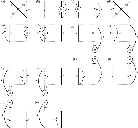
First-order time-ordered diagrams Hugenholtz for \( \boldsymbol{\varPi} \left(\omega \right)-{\boldsymbol{\varPi}}_s\left(\omega \right) \). a–i involve coupling between the particle-hole space; g, h, m, and n involve coupling between particle-hole space and particle-particle; i–l couple the particle-hole space with the hole-hole space


For example, the term corresponding to Fig. 7j is
This brings us to the slightly more difficult treatment of electron repulsions.
-
8.
When electron repulsion integrals are represented by dotted lines (Feynman and Goldstone diagrams), each end of the line corresponds to the labels corresponding to the same spatial point. The dotted line representation may be condensed into points (Abrikosov and Hugenholtz diagrams) as in Fig. 8. A point with two incoming arrows, labeled r and s, and two outgoing arrows, labeled p and q, contributes a factor of \( \left(rs\left|\right|pq\right)=\left(rp\left|{f}_H\right|sq\right)-\left(rq\left|{f}_H\right|sp\right) \). [Thus (in, in | | out, out) = (left in, right in | left in, right in) – (left in, right in | left in, right in). The minus sign is not part of the diagram as it is taken into account by other rules.] The integral notation is established in (29) and the integral
$$ \left(pq\left|\right|rs\right)={\displaystyle \int }{\uppsi}_p^{*}(1){\uppsi}_r^{*}(2)\frac{1}{r_{12}}\left(1-{\mathcal{P}}_{12}\right){\uppsi}_q(1){\uppsi}_s(2) d1d2. $$(57)Fig. 8 
Electron repulsion integral diagrams
-
9.
To determine the number of loops and hence the overall sign of a diagram in which electron repulsion integrals are expanded as dots, write each dot as a dotted line (it does not matter which one of the two in Fig. 8 is chosen) and apply rule 1. The order of indices in each integral \( \left(rs\left|\right|pq\right) \) should correspond to the expanded diagrams. (When Goldstone diagrams are interpreted in this way, we call them Brandow diagrams.)
-
10.
An additional factor of 1/2 must be added for each pair of equivalent lines. These are directed lines whose interchange, in the absence of further labeling, leaves the Hugenholtz diagram unchanged.

For example, the term corresponding to Fig. 7a is
Additional information about Hugenholtz and other diagrams may be found, for example, in [56].
3.3 Dyson’s Equation and the Bethe–Salpeter Equation (BSE)
Two of the most basic equations of diagrammatic MBPT are Dyson’s equation for the one-electron Green’s function and the BSE for the ph-propagator. Both require the choice of a zero-order picture which we take here to be the exact or approximate Kohn–Sham system of noninteracting electrons. We denote the zero-order quantities by the subscript s (for single particle).
Dyson’s equation relates the true one-electron Green’s function G to the zero-order Green’s function G s via the (proper) self-energy Σ,
or, more concisely,
This is shown diagrammatically in Fig. 9. It is to be emphasized that these diagrams are unordered in time as it is not possible to write a Dyson equation for time-ordered diagrams. Also shown in Fig. 9 are typical low-order self-energy approximations. Typical quantum chemistry approximations (Fig. 9b) involve explicit antisymmetrization of electron-repulsion integrals whereas solid-state physics approximations (Fig. 9c) emphasize dynamical screening. Each approach has its strength and its weaknesses and so far the two approaches have defied any rigorous attempts at merger.

Time-unordered (Feynman and Abrikosov) one-electron Green’s function diagrams: (a) Dyson’s equation; (b) second-order self-energy quantum chemistry approximation; (c) GW self-energy solid-state physics approximation
The BSE is “Dyson’s equation” for the ph-propagator,
or
in matrix notation. Here
is the ph-propagator for the zero-order picture (in our case, the exact or approximate Kohn–Sham fictitious system of noninteracting electrons), and the four-point quantity, Ξ Hxc, may be deduced from a Feynman diagram expansion as the proper part of the ph-response function “self-energy”. This is shown diagrammatically in Fig. 10. Again, the quantum chemical approximations emphasize antisymmetrization of the electron repulsion integrals which is needed for proper inclusion of double excitations whereas solid-state physics emphasizes use of a screened interaction. Although no rigorous way is yet known for combining screening and antisymmetrization, an interesting pragmatic suggestion may be found in [57].

Time-unordered (Feynman and Abrikosov) ph-propagator diagrams: (a) BSE; (b) second-order self-energy quantum chemistry approximation; (c) GW self-energy solid-state physics approximation. Note in part (c) that the solid-state physics literature often turns the v and w wiggly lines at right angles to each other to indicate the same thing that we have indicated here by adding tab lines
3.4 Superoperator Equation-of-Motion (EOM) Polarization Propagator (PP) Approach
We now concentrate on the PP and show how to obtain a “Casida-like” equation for excitation energies and transition moments. This does not as yet give us correction terms to AA LR-TD-DFT but it does give us some important tools to help us build correction terms. The basic idea in this section is to take the exact or approximate Kohn–Sham system of independent electrons as the zero-order picture,
to add the perturbation,
and to do MBPT. Here, \( \widehat{V} \) is the fluctuation operator,
and \( {\widehat{\varSigma}}_{\mathrm{x}}^{\mathrm{HF}} \) is the HF exchange operator defined in terms of the occupied Kohn–Sham orbitals. Heuristically this gives us a series of diagrams which we must resum to have the proper analytic structure of the exact PP so we can take advantage of this analytic structure to produce the desired “Casida-like” equation. Rigorously we actually first begin with some exact equations in the superoperator equation-of-motion (EOM) formalism to deduce the analytic structure of the PP. This exact structure is then developed in a perturbation expansion so that we can perform an order analysis of each of the terms entering into a basic “Casida-like” equation. As we can see, not every diagram is generated by this procedure, either because they are not needed or because of approximations which we have chosen to make.
Our MBPT expansions are in terms of the bare electron repulsion (or more exactly the “fluctuation potential” – see (66)), rather than the screened interaction used in solid-state physics [41, 47]. The main advantage of working with the bare interaction is a balanced treatment of direct and exchange diagrams, which is especially important for treating two- and higher-electron excitations. Although we automatically include what the solid state community refers to as vertex effects, the disadvantage of our approach is that it is likely to break down in solids when screening becomes important. The specific approach we take is the now well-established second-order polarization propagator approximation (SOPPA) of Nielsen, Jørgensen, and Oddershede [48–51]. The usual presentation of the SOPPA approach is based upon the superoperator equation-of-motion (EOM) approach previously used by one of us [58]. However, the SOPPA approach is very similar in many ways to the second-order algebraic diagrammatic construction [ADC(2)] approach of Schirmer [52, 53] and we do not hesitate to refer to this approach as needed (particularly with regard to the inclusion of various diagrammatic contributions). The only thing really new here is the change from a Hartree–Fock to a Kohn–Sham zero-order picture and the concomitant inclusion of (many) additional terms. Nevertheless, it is seen that the final working expressions are fairly compact.
Before going into the details of the superoperator EOM approach, let us anticipate some of the results by looking at some of the diagrams which emerge from this analysis. We have seen in (45) that the PP is just the restriction of the ph-propagator to twice rather than four times. Thus, heuristically, it suffices to take the ph-propagator diagrams, fix twice, and then take all possible time orderings. Defining order as the order in the number of times \( \widehat{V} \) and/or \( {\widehat{M}}_{\mathrm{xc}} \) appear, all of the time-unordered first-order terms are shown in Fig. 11. Fixing twice and restricting ourselves to an exchange-only theory gives the 14 time-ordered diagrams shown in Fig. 7. As we can see below in a very precise mathematical way, dangling parts below or above the horizontal dotted lines correspond respectively to Hugenholtz diagrams for initial-time and final-time perturbed wavefunctions. (Two other first-order Goldstone diagrams are found in [52] with the electron repulsion dot above or below the two dotted lines; however a more detailed analysis shows that these terms neatly cancel out in the final analysis.) The area between the dotted lines corresponds to time propagation. In this case, there are only one-hole/one-particle excitations between the two horizontal dotted lines. Our final results are in perfect agreement with diagrams appearing in the exact exchange (EXX) theory as obtained by Hirata et al. [59] which are equivalent to the more condensed form given by Görling [60].

Topologically different first-order time-unordered Abrikosov diagrams for the PP
Figure 12 shows all 13 second-order time-unordered diagrams. Although this may not seem to be very many, our procedure generates about 140 time-ordered Hugenholtz diagrams (and even more Feynman diagrams). A typical time-ordered Hugenholtz diagram is shown in Fig. 13. The corresponding equation,
shows that this diagrams has poles at the double excitations ε ik,ca . Thus we see that the polarization propagator does have poles at double excitations, but we are not really ready to do calculations yet. There are two main reasons: (1) we need a more sophisticated formalism which allows the single and double excitations to mix with each other and (2) we would prefer a (pseudo)eigenvalue equation to solve. Thus we still have to do quite a bit more work to arrive at a “Casida-like” equation with explicit double excitations, but the basic idea is already present in what we have done so far.

Second-order time-unordered Abrikosov PP diagrams. Not all of the time-ordered Hugenholtz diagrams are generated by our procedure – only about 140 Hugenholtz diagrams

An example of a second-order time-ordered Hugenholtz PP diagram
To do so, it is first convenient to express the PP in a molecular orbital basis as
where
As explained in [54], this change of convention with respect to that of (46) turns out to be more convenient. It should also be noted that, because the PP depends only upon the time difference, \( t-t^{\prime } \), we can shift the origin of the time scale so that \( t^{\prime }=0 \) without loss of generality.
Equation (70) can be more easily manipulated by making use of the superoperator formalism. A (Liouville-space) superoperator \( \overset{\smile }{X} \) is defined by its action on a (Hilbert-space) operator  as
When \( \overset{\smile }{X} \) is the Hamiltonian operator, \( \overset{\smile }{H} \), one often speaks of the Liouvillian. An exception is the identity superoperator, \( \overset{\smile }{1} \), whose action is simply given by
The Heisenberg form of orbital creation and annihilation operators is easily expressed in terms of the Liouvillian superoperator,
Then
Taking the Fourier transform (with appropriate convergence factors (not shown)) gives,
where we have introduced the superoperator metric,Footnote 7
[It may be useful to note that
follows as an easy consequence of the above definitions. Moreover, because we typically use real orbitals and a finite basis set, the PP is a real symmetric matrix. This allows us simply to identify Π as the superoperator resolvant,
Because matrix elements of a resolvant superoperator are harder to manipulate than resolvants of a superoperator matrix, we transform (75) into the later form by introducing a complete set of excitation operators. The complete set
leads to the resolution of the identity (RI):
We have defined the operator space differently from the previous work of one of us [38] to be more consistent with the literature on the field of PP calculations. The difference is actually the commutation of two operators which introduces one sign change. Insertion into (75) and use of the relation
then gives
This shows us the analytical form of the exact polarization propagator.
The corresponding “Casida-like” pseudoeigenvalue equation is
and with normalization
Let us also seek a sum-over-states expression for the polarization propagator.
Spectral expansion tells us that
and
So (82) reads
This means that the PP has poles given at the pseudoeigenvalues of (83) and that the eigenvectors may be used to calculate oscillator strengths via (87).
As the “Casida-like” (83) is so important, let us rewrite it as
which is roughly
The A and B matrices, as well as the X and Y, partition according to whether they refer to one-electron excitations or two-electron excitations. In the Tamm–Dancoff approximation the B matrices are neglected so we can write
Here X has been replaced by C as is traditional and to reflect the normalization \( {\mathbf{C}}^{\dagger}\mathbf{C}=1 \).
The superscripts in (91) reflect a somewhat difficult order analysis which is carried out in the Appendix. This analysis consists of expanding the polarization propagator algebraically and then matching each term to a set of diagrams to see what order of each EOM matrix is needed to get a given order of polarization propagator.
The result in the case of the A matrices is
where \( {F}_{r,s}^{\left(0+1\right)}={\delta}_{r,s}{\varepsilon}_r+{M}_{r,s}^{xc} \) is the matrix of the Hartree–Fock operator constructed with Kohn–Sham orbitals and
include second-order corrections. (Note that extra factors of 1/2 occur in these expressions when spin is taken explicitly into account.) In practice, a zero-order approximation to A 2,2 is insufficient and we must use an expression correct through first order:
where
We refer to the resultant method as extended SOPPA/ADC(2). It is immediately seen that truncating to first order recovers the usual configuration interaction singles (CIS) equations in a noncanonical basis set. We now have the essential tools to proceed with the rest of this chapter.
4 Dressed LR-TD-DFT
We now give one answer to the problem raised in the introduction – how to include explicit double excitations in LR-TD-DFT. This answer goes by the name “dressed LR-TD-DFT” and consists of a hybrid MBPT/AA LR-TD-DFT method. We first give the basic idea and comment on some of the early developments. We then go into the practical details which are needed to make a useful implementation of dressed LR-TD-DFT. Finally, we introduce the notion of Brillouin corrections which are undoubtedly important for photochemistry.
4.1 Basic Idea
As emphasized in Sect. 2, simple counting arguments show that the AA limits LR-TD-DFT to single excitations, albeit dressed to include some electron correlation. However, explicit double excitations are sometimes needed when describing excited states. This was discussed in the introduction in the context of photochemistry (Fig. 1). It is well known in ab initio quantum chemistry that double excitations can be important when describing vertical excitations and the best known example is briefly discussed in the caption of Fig. 14.

Doubles contribution to the 1 A g excited state of butadiene. Beecause the obvious two lowest singly-excited singlets 1(1b g , 2b g ) and 1(1a u , 2a u ) are quasidegenerate in energy, they mix to form new singly-excited singlets \( \Big(1/\sqrt{\Big(}{2\left)\right)\Big[}^1\left(1{b}_g,2{b}_g\right){\pm}^1\left(1{a}_u,2{a}_u\right)\Big] \). One of these is quasidegenerate with the doubly-excited singlet dark state 1(1b 2 g , 2a 2 u ). The resultant mixing modifies the energy and intensity of the observed 1 A g excited state
At first this may seem a little perplexing because the fact that the oscillator strength is the transition matrix element of a one-electron operator – see (15) – means that the oscillator strength of a double excitation relative to a single-determinantal ground-state wavefunction should be zero – that is, the doubly excited state should be spectroscopically dark. What happens is easily explained by the two-level model shown in Fig. 15, which is sufficient to give a first explanation of the butadiene case, for example. (In the butadiene case, the singly-excited state to be used is already a mixture of two different one-hole/one-particle states.) Figure 15 shows a bright singly-excited state with excitation energy ω S and oscillator strength \( {f}_S=1 \) interacting with a dark doubly-excited state with excitation energy ω D and oscillator strength \( {f}_D=0 \) via a coupling matrix element x. The CI problem is simply
which can be formally solved, obtaining
for some value of θ. It should be noted that the average excitation energy is conserved in the coupled problem (\( {\omega}_a+{\omega}_b={\omega}_S+{\omega}_D \)) and that something similar occurs with the oscillator strengths. This leads to the common interpretation that the coupling “shatters the singly-excited peaks into two satellite peaks.”

Two-level model used by Maitra et al. in their heuristic derivation of dressed TDDFT. See explanation in text
Now let us see how this wavefunction theory compares with LR-TD-DFT and how Maitra et al. [61] decided to combine the two into a hybrid method. Of course, the proper comparison with CI is LR-TD-DFT within the TDA. Applying the partitioning technique to (95), we obtain
Comparing this with the diagonal TDA LR-TD-DFT within the two-orbital model,
shows that
Maitra et al. [61] interpreted the first term as the adiabatic part,
and second term as the nonadiabatic correction,
Additionally, it is easy to show that
which is the form of the numerator used by Maitra et al. [61]. The suggestion of Maitra et al., which defines dressed LR-TD-DFT, is to calculate the nonadiabatic correction terms – see (101) – from MBPT [61]. Thus x and ω D in (95) are to be calculated using MBPT rather than using DFT.
4.2 Practical Details and Applications
Applications of dressed LR-TD-DFT to the butadiene and related problems have proven to be very encouraging [61–64]. Nevertheless, several things were missing in these seminal papers. In the first place, they did not always use exactly the same formalism for dressed LR-TD-DFT and not always the same DFAs. Moreover, although the formalism showed encouraging results for a few molecules for those excitations which were thought to be most affected by explicit inclusion of double excitations, the same references failed to show that predominantly single excitations were left largely unaffected by the dressing of AA LR-TD-DFT. These questions were carefully addressed in [65], with some surprising answers.
The implementation of dressed LR-TD-DFT considered in [65] was to add just a few double excitations to AA LR-TD-DFT and solve the TDA equation
Thus the calculation of the A 1,1 block, which is one of the most difficult to calculate in the extended SOPPA/ADC(2) theory, is very much simplified by using AA LR-TD-DFT. The A 2,2 block must, however, be calculated through first order in practice. It was confirmed that adding only a few (e.g., 100) double excitations led to little difference in calculated eigenvalues unless the double excitations were quasidegenerate with a single excitation. There is thus no significant problem in practice with double counting electron correlation effects when using this hybrid MBPT/LR-TD-DFT method. Tests were carried out on the test set of Schreiber et al. consisting of 28 organic chromophores with 116 well-characterized singlet excitation energies [66].
Note that the form of (103) was chosen instead of the form
for computational simplicity. However, (104) is the straightforward extension of the dressed kernel given at the end of the previous section and is easy to generalize to the full response theory case (i.e., without making the TDA).
We confirm the previous report that using the LDA for the AA LR-TD-DFT part of the calculation often gives good agreement with vertical excitation energies having significant double excitation contributions [67]. However, most excitations are dominated by singles and these are significantly underestimated by the AA LDA. Inclusion of double excitations tended to decrease the typically already too low AA LDA excitation energy. The AA LR-TD-DFT block was then modified to behave in the same way as a global hybrid functional with 20% Hartree–Fock exchange. The excitations with significant doubles character were then found to be overestimated but the addition of the doubles MBPT contribution again gave good agreement with benchmark ab initio results. This was consistent with previous experience with dressed LR-TD-DFT [61–64]. The real surprise was the discovery that adding the MBPT to the hybrid functional made very little difference for the majority of excitations which are dominated by single excitation character. It thus seems that a dressed LR-TD-DFT requires the use of hybrid functional.
4.3 Brillouin Corrections
So far, dressed LR-TD-DFT allows us to include explicit double excitations and so to describe photochemical funnels between excited states. However, a worrisome point remains, namely how to include doubles contributions to the ground state in the same way that we include doubles contributions to excited states so that we may describe, for example, the photochemical funnel between S1 and S0 in Fig. 1. It is not clear how to do this in LR-TD-DFT where the excited-state potential energy surfaces are just obtained by adding the excitation energies at each geometry to the ground-state DFT energies. Not only does such a procedure lead to the excited states inheriting the convergence difficulties of the ground state surface coming from places with noninteracting v-representability difficulties, but also there is no coupling between the ground state and singly excited states. This is similar to what happens with Brillouin’s theorem in CIS calculations and leads to problems describing conical intersections. However, adding in the missing nonzero terms (which we call Brillouin corrections) to dressed LR-TD-DFT is easy in the TDA.
It is good to emphasize at this point that we are making an ad hoc correction, albeit one which is eminently reasonable from a wavefunction point of view. Formally correct approaches might include: (1) acknowledging that part of the problem may lie in the fact that noninteracting v-representability in Kohn–Sham DFT often breaks down at key places on ground-state potential energy surfaces when bonds are formed or broken, so that conventional Kohn–Sham DFT may no longer be a good starting point; (2) examining nonadiabatic xc-kernels which seem to include some degree of multideterminantal ground-state character in their response such as that of Maitra and Tempel [68]; (3) introducing explicit multideterminantal character into the description of the Kohn–Sham DFT ground state. We return to this in our final section, but for now we just try the ad hoc approach of adding Brillouin corrections to TDA dressed LR-TD-DFT. Note that this also has an indirect effect on interactions between excited states, though the primary effect is between excited states and the ground state.
It is sufficient to add an extra column and row to the TDA problem to take into account the ground-state determinant in hybrid DFT. This gives
where the extra matrix elements are calculated as
and
Of course, we can also derive a corresponding nonadiabatic correction to the xc-coupling matrix:
The extension beyond the TDA is not obvious in this case.
4.3.1 Dissociation of Molecular Hydrogen
Molecular hydrogen dissociation is a prototypical case where doubly-excited configurations are essential for describing the potential energy surfaces of the lowest-lying excited states. The three lowest singlet states of \( {\varSigma}_g^{+} \) symmetry can be essentially described by three CI configurations, namely (1σ 2 g 1σ 0 u 2σ 0 g ), (1σ 1 g 1σ 0 u 2σ 1 g ), and (1σ 0 g 1σ 2 u 2σ 0 g ), referred to as ground, single, and double configuration, respectively.
Obviously, the double configuration plays an essential role when a restricted single-determinant is used as reference. On the one hand, the mixing of ground and double configurations is necessary for describing the correct −1 Hartree dissociation energy of H2. On the other hand, the single and double configurations mix at around 2.3 bohr, thus producing an avoided crossing. These features are shown in Fig. 16, where we compare different flavors of TD-DFT with the CISD benchmark (shown as solid lines in all graphs).

Potential energy surfaces of the ground and two lowest excited states of \( {\varSigma}_{\mathrm{g}}^{+} \) symmetry. Comparison of CISD (solid lines) with adiabatic, dressed, and hybrid LR-TD-BH&HLYP/TDA (dashed lines). All calculations have been performed with a cc-pVTZ basis set. All axes are in Hartree atomic units (bohr for the x-axis and Hartree for the y-axis). Unlike the ethylene potential energy curves (Fig. 17), no shift has been made in the potential energy curves
Adiabatic TD-DFT (shown in Fig. 16a) misses completely the double configuration, and so neither the avoided crossing nor the dissociation limit is described correctly. It should be noted, however, that CISD and adiabatic TD-DFT curves are superimposed for states X \( {}^1{\varSigma}_g^{+} \) and 1 \( {}^1{\varSigma}_g^{+} \) at distances lower than 2.3 bohr, where the KS assumption is fully satisfied. At distances larger than 2.3 bohr, the 1 \( {}^1{\varSigma}_g^{+} \) state corresponds to the CISD 2 \( {}^1{\varSigma}_g^{+} \) state. This is because the 1 \( {}^1{\varSigma}_g^{+} \) in TD-DFT is diabatic, as it does not contain the doubly-excited configuration. The dissociation limit is also overestimated as it is usual from RKS with common xc functionals.
Dressed TD-DFT (Fig. 16b) includes the double configuration. On the one hand, the avoided crossing is represented correctly. However, the gap between the \( {1}^1{\varSigma}_g^{+} \) and the \( {2}^1{\varSigma}_g^{+} \) is smaller than the CISD crossing. The dissociation limit, however, is not correctly represented, as dressed TD-DFT does not include the ground- to excited-state interaction. Therefore, the double configuration dissociates at the same limit as the ground configuration.
Brillouin dressed TD-DFT (Fig. 16b) also includes the ground- and double configuration mixture additional to the single- and double mixing of dressed TD-DFT. On the one hand, the avoided crossing is represented more precisely, with a gap closer to that of CISD. Now the dissociation limit is more correctly described. Still there is a slight error in the dissociation energy limit, probably because of the double counting of correlation. This could be alleviated by a parameterization of the Brillouin-corrected dressed TD-DFT functional.
4.3.2 Ethylene Torsion
In Fig. 17 we show the potential energy surfaces of S0, S1, and S2 of ethylene along the torsional coordinate. The static correlation of these three states can be essentially represented by three configurations, namely the ground-state configuration (π2π*,0), the singly-excited configuration (π1π*,1), and the doubly-excited configuration (π0π*,2).

Potential energy cuts of the S0, S1, and S2 states of ethylene along the twisting coordinate: x-axis in degrees, y-axis in eV. All the curves have been shifted so that the ground-state curve at 0° corresponds to 0 eV. The solid lines correspond to a CASSCF(2,2)/MCQDPT2 calculation, and the dashed lines to the different models using the BH&HLYP functional and the Tamm–Dancoff approximation. The 6-31++G(d,p) basis set have been employed in all calculations. (Note that these curves are in good agreement with similar calculations previously reported in Fig. 7.3 of Chap. 7 of [69], albeit with a different functional)
From the CASSCF(2,2)/MCQDPT2, we observe that the ground- and doubly-excited configurations are heavily mixed at 90°, forming an avoided crossing. At this angle, the S1 and S2 states are degenerate. These features are not captured by adiabatic TD-DFT (Fig. 17a). Indeed, the doubly-excited configuration is missing, and so the ground state features a cusp at the perpendicular conformation. The S1, which is essentially represented by a single excitation, is virtually superimposed with the CASSCF(2,2)/MCQDPT2 result. The dressed TD-DFT (Fig. 17b) includes the double excitation, but the surfaces of S0 and S2 appear as diabatic states because the ground- to excited-state coupling term is missing. This is largely fixed by introducing the Brillouin corrections (Fig. 17c). The ground state is now in very good agreement with the CASSCF(2,2)/MCQDPT2 S0 state, although the degeneracy of S1 and S2 at 90° is still not fully captured. Thus the picture given by Brillouin-corrected LR-TD-DFT is qualitatively correct with respect to the multi-reference results.
5 Effective Exchange-Correlation (xc) Kernel
We now have the tools to deduce an MBPT expression for the TD-DFT xc-kernel. It should be emphasized that this is not a new exercise but that we seem to be the only ones to do so within the PP formalism. We think this may have the advantage of making a rather complicated subject more accessible to Quantum Chemists already familiar with the PP formalism.
The problem of constructing xc-correlation objects such as the xc-potential v xc and the xc-kernel f xc(ω) from MBPT for use in DFT has been termed “ab initio DFT” by Bartlet [70, 71]. At the exchange-only level, the terms optimized effective potential (OEP) [72, 73] or exact exchange [74, 75] are also used and OEP is also used to include the correlated case [76, 77]. At first glance, nothing much is gained. For example, the calculated excitation energies and oscillator strengths in ab initio TD-DFT must be, by construction, exactly the same as those from MBPT. This approach does not give explicit functionals of the density (though it may be thought of as giving implicit functionals). However it does allow us to formulate expressions for and to calculate purely (TD-) DFT objects and hence it can provide insight into, and computational checks of, the behavior of illusive objects such as v xc and f xc(ω).
Here we concentrate on the latter, namely the xc-kernel. Previous work along these lines has been carried out for the kernel by directly taking the derivative of the OEP energy expression with the constraint that the orbitals come from a local potential. This was first done by Görling in 1998 [60] for the full time-dependent exchange-only problem. In 2002, Hirata et al. redid the derivation for the static case [78]. Later, in 2006, a diagrammatic derivation of the static result was given by Bokhan and Bartlett [71], and the functional derivative of the kernel g x has been treated by Bokhan and Bartlett in the static exchange-only case [79].
In this section, we take a somewhat different and arguably more direct approach than that used in the previously mentioned articles, in that we make direct use of the fundamental relation
where \( {\mathbf{i}}^{+} \) is infinitesimally later than i. This approach has been used by Totkatly, Stubner, and Pankaratov to develop a diagrammatic expression for f xc(ω) [80, 81]. It also leads to the “Nanoquanta approximation,” so named by Lucia Reining because it was simultaneously derived by several different people [41–43, 46, 44] involved in the so-called Nanoquanta group. (See also pp. 318–329 of [24].)
The work presented here differs from previous work in two respects, namely (1) we make a direct connection with the PP formalism which is more common in quantum chemistry than is the full BSE approach (they are formally equivalent but differ in practice through the approximations used) and (2) we introduce a matrix formulation based upon Harriman’s contraction \( \widehat{\varUpsilon} \) and expansion operators \( {\widehat{\varUpsilon}}^{\dagger } \). This allows us to introduce the concept of the localizer Λ(ω) which shows explicitly how localization in space results requires the introduction of additional frequency dependence. Finally, we recover the formulae of Görling and Hirata et al. and produce a rather trivial proof of the Gonze and Scheffler result [82] that this additional frequency dependence “undoes” the spatial localization procedure in particular cases.
We first seek a compact notation for (109). Harriman considered the relation between the space of kernels of operators and the space of functions [83, 84]. In order to main consistency with the rest of this chapter, we generalize Harriman’s notion from space-only to space and spin coordinates. Then the collapse operator is defined by
for an arbitrary operator kernel. The adjoint of the collapse operator is the so-called expansion operator
for an arbitrary function f(1). Clearly \( {\widehat{\varUpsilon}}^{\dagger}\widehat{\varUpsilon}A\left(1,2\right)=A\left(1,1\right)\delta \left(1-2\right)\ne A\;\left(1,2\right) \). The ability to express these operators as matrices (ϒ and ϒ †) facilitates finite basis set applications.
We may now rewrite (109) as
Comparing
with the BSE
or, more precisely, with
then shows that
If we take advantage of the Kohn–Sham reference giving us the exact density, then the Hartree part cancels out so that we actually get
Although this is certainly a beautiful result, it is nevertheless plagued with four-time quantities which may be eliminated by using the PP:
where we have introduced the coupling matrix defined by
The price we have to pay is that the coupling matrix cannot be easily expanded in Feynman diagrams, but that in no way prevents us from determining appropriate algebraic expressions for it. We may then write
which Fourier transforms to remove all the integrations,
5.1 Localizer
Evidently,
where we have introduced the notion of noninteracting (Λ s ) and interacting (Λ) localizers,
The localizer arises quite naturally in the context of the time-dependent OEP problem. According to the Runge–Gross theory [25], the exact time-dependent xc-potential v xc(t) is not only a functional of the density ρ(t) but also of an initial condition which can be taken as the wavefunction Ψ(t 0) at some prior time t 0. On the other hand, linear response theory begins with the static ground state case where the first Hohenberg–Kohn theorem tells us that the wavefunction is a functional of the density \( \Psi \left({t}_0\right)=\Psi \left[{\rho}_{t_0}\right] \). Görling has pointed out that this greatly simplifies the problem [60] because we can then show that
where Σ x is the Hartree–Fock exchange operator. Equivalently, this may be written as
or Σ x ,
Equations (122) and (126) are telling us something of fundamental importance, namely that the very act of spatially localizing the xc-coupling matrix involves introducing additional frequency dependence.
For the special case of noninteracting susceptibility, we can easily derive an expression for the dynamic localizer. Because
we can express the kernel of ϒ Π s (ω) as
Also, the kernel of ϒ Π s (ω)ϒ † is just
As with the susceptibility, the two operators have poles at the independent particle excitation energies \( \omega =\pm {\varepsilon}_{a,i}=\pm \left({\varepsilon}_a-{\varepsilon}_i\right) \).
In order to construct the dynamic localizer, the kernel (125) has to be inverted. It is not generally possible to do this analytically, though it can be done in a finite-basis representation with great care. However, Gonze and Scheffler have noted that exact inversion is possible in the special case of a frequency, \( \omega ={\varepsilon}_{b,j} \), of a pole well separated from the other poles [82]. Near this pole, the kernels, ϒΠ s (ω) and ϒΠ s (ω)ϒ †, are each dominated by single terms
Thus (125) becomes
with the approximation becoming increasingly exact as ω approaches ε b,j . Hence,
More generally for an arbitrary dynamic kernel, K(1, 2; ω),
and we can do the same for \( -{\varepsilon}_{b,j} \), obtaining
We refer to these last two equations as Gonze–Scheffler (GS) relations, because they were first derived by these authors [82] and because we want to use them again. These GS relations show that the dynamic localizer, Λ s (ω), is pole free if the excitation energies, ε a,i , are discrete and nondegenerate and suggest that the dynamic localizer may be a smoother function of ω than might at first be suspected. Equation (132) is also very significant because we see that, at a particular frequency, the matrix element of a local operator is the same as the matrix element of a nonlocal operator. Generalization to the xc-kernel requires an approximation.
5.1.1 First Approximation
Equation (122) is difficult to solve because of the need to invert an expression involving the correlated PP. However, it may instead be removed by using the approximate expression
where a localizer is used which is half way between the noninteracting and fully interacting form,
Equation (135) then becomes
Such an approximation is expected to work well in the off-resonant regime. As we can see, it does give Görling’s exact exchange (EXX) kernel for TD-DFT [60]. On the other hand, the poles of the kernel in this approximation are a priori the poles of the exact and independent particle PPs – that is, the true and single-particle excitation energies – unless well-balanced approximations lead to fortuitous cancellations.
We can now return to a particular aspect of Casida’s original PP approach [58] which was failure to take proper account of the localizer. This problem is rectified here. The importance of the localizer is made particularly clear by the GS relations in the case of charge transfer excitations. The single-pole approximation to the \( i\to a \) excitation energy is
Thus once again we see that the frequency dependence of the localizer has transformed the matrix element of a spatially-local frequency-dependent operator into the matrix element of a spatially-nonlocal operator. Had the localizer been neglected, then we would have found, incorrectly, that
Although the latter reduces to just ε ai for charge transfer excitations at a distance (because \( {\uppsi}_i{\uppsi}_a=0 \)), the former does not [85]. However, for most excitations the overlap is non-zero. In such cases, and around a well-separated pole, the localizer can be completely neglected.
5.1.2 Exchange-Only Case
In order to apply (137) we need only the previously derived terms represented by the diagrams in Fig. 7. The resultant expressions agree perfectly with the expanded expressions of the TD-EXX kernel obtained by Hirata et al. [59], which are equivalent to the more condensed form given by Görling [60].
Use of the GS relation then leads to
which is exactly the configuration interaction singles (CIS, i.e., TDHF Tamm–Dancoff approximation) expression evaluated using Kohn–Sham orbitals. This agrees with a previous exact result obtained using Görling–Levy perturbation theory [82, 86, 87].
5.1.3 Second Approximation
A second approximation, equivalent to the PP Born approximation,
is useful because of its potential for preserving as much as possible of the basic algebraic structure of the exact equation at (122) although still remaining computationally tractable. This is our second approximation,
Equation (142) simply reads that f Hxc(ω) is a spatially localized form of K Hxc(ω). This is nothing but the PP analogue of the basic approximation (117) used in the BSE approach on the way to the Nanoquanta approximation [41–46].
6 Conclusion and Perspectives
Time-dependent DFT has become part of the photochemical modeler’s toolbox, at least in the FC region. However, extensions of TD-DFT are being made to answer the photochemical challenge of describing photochemical funnel regions where double and possibly higher excitations often need to be taken into account. This chapter has presented the dressed TD-D FT approach of using MBPT corrections to LR-TD-DFT in order to help address problems which are particularly hard for conventional TD-DFT. Illustrations have been given for the dissociation of H2 and for cis/trans isomerization of ethylene. We have also included a section deriving the form of the TD-DFT xc-kernel from MBPT. This derivation makes it clear that localization in space is compensated for in the exact kernel by including additional frequency dependences. In the short run, it may be that such additional frequency dependences are easier to model with hybrid MBPT/LR-TD-DFT approaches. Let us mention in closing the very similar “configuration interaction-corrected Tamm–Dancoff approximation” of Truhlar and coworkers [88]. Yet another approach, similar in spirit, but different in detail is multiconfiguration TD-DFT based upon range separation [89]. In the future, if progress continues to be made at the current rate, we may very well be using some combination of these, including elements of dressed LR-TD-DFT, as well as other tricks such as a Maitra–Tempel form of the xc-kernel [68], constricted variational DFT for double excitations [90], DFT multi-reference configuration interaction (DFT-MRCI) [91], spin-flip theory [92–102], and restricted open-shell or spin-restricted ensemble-referenced Kohn–Sham theory [97, 100, 101, 103–105] to attack difficult photochemical problems on a routine basis. Key elements to make this happen are the right balance between rigor and practicality, ease of automation, and last but not least ease of use if many users are going to try these techniques and if they can be routinely applied at every time step of a photochemical dynamics simulation.
Notes
- 1.
The term ab initio is used here as it is typically used in quantum chemistry. That is, ab initio refers to first-principles Hartree–Fock-based theory, excluding DFT. In contrast, the term ab initio used in the solid state physics literature usually encompasses DFT.
- 2.
“Jacob set out from Beersheba and went on his way towards Harran. He came to a certain place and stopped there for the night, because the sun had set; and, taking one of the stones there, he made it a pillow for his head and lay down to sleep. He dreamt that he saw a ladder, which rested on the ground with its top reaching to heaven, and angels of God were going up and down it.” – The Bible, Genesis 28:10–13
- 3.
This is formalized in mathematical logic theory by Gödel’s incompleteness theorem which basically says that there are always more things that are true than can be proven to be true.
- 4.
Remember that ℏ = 1 in the atomic units used here.
- 5.
This equation is not infrequently called the “Casida equation” in the TD-DFT literature (e.g., as in [24], pp. 145–153.)
- 6.
Sometimes we call this the FORTRAN index convention in reference to the default variable names for integers in that computer language.
- 7.
Technically this is not a metric, because the overlap matrix is symplectic rather than positive definite. However, we will call it a metric as it can be used in much the same way as a true metric.
References
Rowlinson JS (2009) The border between physics and chemistry. Bull Hist Chem 34:1
Casida ME, Jamorski C, Casida KC, Salahub DR (1998) Molecular excitation energies to high-lying bound states from time-dependent density-functional response theory: characterization and correction of the time-dependent local density approximation ionization threshold. J Chem Phys 108:4439
Casida ME (2002) Jacob’s ladder for time-dependent density-functional theory: some rungs on the way to photochemical heaven. In: Hoffmann MRH, Dyall KG (eds) Accurate description of low-lying molecular states and potential energy surfaces. ACS, Washington, p 199
Doltsinis NL, Marx D (2002) First principles molecular dynamics involving excited states and nonadiabatic transitions. J Theo Comput Chem 1:319
Cordova F, Doriol LJ, Ipatov A, Casida ME, Filippi C, Vela A (2007) Troubleshooting time-dependent density-functional theory for photochemical applications: oxirane. J Chem Phys 127:164111
Tapavicza E, Tavernelli I, Rothlisberger U, Filippi C, Casida ME (2008) Mixed time-dependent density-functional theory/classical trajectory surface hopping study of oxirane photochemistry. J Chem Phys 129(12):124108
Casida ME, Natarajan B, Deutsch T (2011) Non-Born-Oppenheimer dynamics and conical intersections. In: Marques M, Maitra N, Noguiera F, Gross EKU, Rubio A (eds) Fundamentals of time-dependent density-functional theory, Lecture Notes in Physics, vol 837. Springer, Berlin, p 279
Casida ME, Huix-Rotllant M (2012) Progress in time-dependent density-functional theory. Annu Rev Phys Chem 63:287
Hohenberg P, Kohn W (1964) Inhomogenous electron gas. Phys Rev 136:B864
Kohn W, Sham LJ (1965) Self-consistent equations including exchange and correlation effects. Phys Rev 140:A1133
Parr RG, Yang W (1989) Density-functional theory of atoms and molecules. Oxford University Press, New York
Dreizler DM, Gross EKU (1990) Density functional theory, an approach to the quantum many-body problem. Springer, New York
Koch W, Holthausen MC (2000) A chemist’s guide to density functional theory. Wiley-VCH, New York
Perdew JP, Schmidt K (2001) Jacob’s ladder of density functional approximations for the exchange-correlation energy. In: Doren VEV, Alseoy KV, Geerlings P (eds) Density functional theory and its applications to materials. American Institute of Physics, Melville, New York, p 1
Perdew JP, Ruzsinsky A, Constantin LA, Sun J, Csonka GI (2009) Some fundamental issues in ground-state density functional theory: a guide for the perplexed. J Chem Theor Comput 5:902
Perdew JP, Constantin LA (2007) Laplacian-level density functionals for the kinetic energy density and exchange-correlation energy. Phys Rev B 75:155109
Gill PM (2001) Obituary: density-functional theory (1927–1993). Aust J Chem 54:661
Becke A (1993) A new mixing of HartreeFock and local density functional theories. J Chem Phys 98:1372
Perdew JP, Ernzerhof M, Burke K (1996) Rationale for mixing exact exchange with density functional approximations. J Chem Phys 105:9982
Savin A (1995) Beyond the Kohn–Sham determinant. In: Chong DP (ed) Recent advances in density functional theory. World Scientific, Singapore, p 129
Baer R, Livshits E, Salzner U (2010) Tuned range-separated hybrids in density functional theory. Annu Rev Phys Chem 61:85
Marques MAL, Ullrich C, Nogueira F, Rubio A, Gross EKU (eds) (2006) Time-dependent density-functional theory, Lecture Notes in Physics, vol 706. Springer, Berlin
Marques M, Maitra N, Noguiera F, Gross EKU, Rubio A (2011) Fundamentals of time-dependent density-functional theory, Lecture Notes in Physics, vol 837. Springer, Berlin
Ullrich CA (2012) Time-dependent density-functional theory: concepts and applications. Oxford University Press, Oxford
Runge E, Gross EKU (1984) Density functional theory for time-dependent systems. Phys Rev Lett 52:997
van Leeuwen R (1999) Mapping from densities to potentials in time-dependent density-functional theory. Phys Rev Lett 82:3863
Maitra NT, Todorov TN, Woodward C, Burke K (2010) Density-potential mapping in time-dependent density-functional theory. Phys Rev A 81:042525
Ruggenthaler M, van Leeuwen R (2011) Global fixed-point proof of time-dependent density-functional theory. Europhys Lett 95:13001
Ruggenthaler M, Glesbertz KJH, Penz M, van Leeuwen R (2012) Density-potential mappings in quantum dynamics. Phys Rev A 85:052504
Ruggenthaler M, Nielsen SEB, van Leeuwen R (2013) Analytic density functionals with initial-state dependence. Phys Rev A 88:022512
Vignale G (2008) Real-time resolution of the causality paradox of time-dependent density-functional theory. Phys Rev A 77(6):1. doi:10.1103/PhysRevA.77.062511
Messud J, Dinh PM, Reinhard P, Suraud E (2011) The generalized SIC-OEP formalism and the generalized SIC-Slater approximation (stationary and time-dependent cases). Ann Phys (Berlin) 523:270
Rajagopal AK (1996) Time-dependent variational principle and the effective action in density-functional theory and Berrys phase. Phys Rev A 54:3916
van Leeuwen R (1998) Causality and symmetry in time-dependent density-functional theory. Phys Rev Lett 80:1280
van Leeuwen R (2001) Key concepts in time-dependent density-functional theory. Int J Mod Phys 15:1969
Mukamel S (2005) Generalized time-dependent density-functional-theory response functions for spontaneous density fluctuations and nonlinear response: resolving the causality paradox. Phys Rev A 024503
Mosquera MA (2013) Action formalism in time-dependent density-functional theory. Phys Rev B 88:022515
Casida ME (1995) Time-dependent density-functional response theory for molecules. In: Chong DP (ed) Recent advances in density functional methods, Part I. World Scientific, Singapore, p 155
Casida ME (1996) Time-dependent density functional response theory of molecular systems: theory, computational methods, and functionals. In: Seminario J (ed) Recent developments and applications of modern density functional theory. Elsevier, Amsterdam, p 391
Löwdin PO (1964) Studies in perturbation theory. Part VI. Contraction of secular equations. J Mol Spectr 14:112
Onida G, Reining L, Rubio A (2002) Electronic excitations: density-functional versus many-body Greens-function approaches. Rev Mod Phys 74:601
Reining L, Olevano V, Rubio A, Onida G (2002) Excitonic effects in solids described by time-dependent density-functional theory. Phys Rev Lett 88:066404
Sottile F, Olevano V, Reining L (2003) Parameter-free calculation of response functions in time-dependent density-functional theory. Phys Rev Lett 91:056402
Marini A, Sole RD, Rubio A (2003) Bound excitons in time-dependent density-functional theory: optical and energy-loss spectra. Phys Rev Lett 91:256402
Stubner R, Tokatly IV, Pankratov O (2004) Excitonic effects in time-dependent density-functional theory: an analytically solvable model. Phys Rev B 70:245119
von Barth U, Dahlen NE, van Leeuwen R, Stefanucci G (2005) Conserving approximations in time-dependent density functional theory. Phys Rev B 72:235109
Romaniello P, Sangalli D, Berger JA, Sottile F, Molinari LG, Reining L, Onida G (2009) Double excitations in finite systems. J Chem Phys 130:044108
Oddershede J, Jørgensen P (1977) An order analysis of the particle-hole propagator. J Chem Phys 66:1541
Nielsen ES, Jørgensen P, Oddershede J (1980) Transition moments and dynamic polarizabilities in a second order polarization propagator approach. J Chem Phys 73:6238
Nielsen ES, Jørgensen P, Oddershede J (1980) J Chem Phys 75:499; Erratum (1980): J Chem Phys 73:6238
Jørgensen P, Simons J (1981) Second quantization-based methods in quantum chemistry. Academic, New York
Schirmer J (1982) Beyond the random phase approximation: a new approximation scheme for the polarization propagator. Phys Rev A 26:2395
Trofimov AB, Stelter G, Schirmer J (1999) A consistent third-order propagator method for electronic excitation. J Chem Phys 111:9982
Fetter AL, Walecka JD (1971) Quantum theory of many-particle systems. McGraw-Hill, New York
Kobe DH (1966) Linked cluster theorem and the Green’s function equations of motion for a many-fermion system. J Math Phys 7(10):1806
Wilson S (1984) Electron correlation in molecules. Clarendon, Oxford
Sangalli D, Romaniello P, Colò G, Marini A, Onida G (2011) Double excitation in correlated systems: a many-body approach. J Chem Phys 134:034115
Casida ME (2005) Propagator corrections to adiabatic time-dependent density-functional theory linear response theory. J Chem Phys 122:054111
Hirata S, Ivanov S, Bartlett RJ, Grabowski I (2005) Exact-exchange time-dependent density-functional theory for static and dynamic polarizabilities. Phys Rev A 71:032507
Görling A (1998) Exact exchange kernel for time-dependent density-functional theory. Int J Quant Chem 69:265
Maitra NT, Zhang F, Cave RJ, Burke K (2004) Double excitations within time-dependent density functional theory linear response theory. J Chem Phys 120:5932
Cave RJ, Zhang F, Maitra NT, Burke K (2004) A dressed TDDFT treatment of the 1Ag states of butadiene and hexatriene. Chem Phys Lett 389:39
Mazur G, Włodarczyk R (2009) Application of the dressed time-dependent density functional theory for the excited states of linear polyenes. J Comput Chem 30:811
Gritsenko OV, Baerends EJ (2009) Double excitation effect in non-adiabatic time-dependent density functional theory with an analytic construction of the exchange-correlation kernel in the common energy denominator approximation. Phys Chem Chem Phys 11:4640
Huix-Rotllant M, Ipatov A, Rubio A, Casida ME (2011) Assessment of dressed time-dependent density-functional theory for the low-lying valence states of 28 organic chromophores. Chem Phys 391:120
Schreiber M, Silva-Junior MR, Sauer SPA, Thiel W (2008) Benchmarks for electronically excited states: CASPT2, CC2, CCSD, and CC3. J Chem Phys 128:134110
Hsu CP, Hirata S, Head-Gordon M (2001) Excitation energies from time-dependent density functional theory for linear polyene oligomers: butadiene to decapentaene. J Phys Chem A 105:451
Maitra NT, Tempel DG (2006) Long-range excitations in time-dependent density functional theory. J Chem Phys 125:184111
Huix-Rotllant M (2011) Improved correlation kernels for linear-response time-dependent density-functional theory. Ph.D. thesis, Université de Grenoble
Bokhan D, Schweigert IG, Bartlett RJ (2005) Interconnection between functional derivative and effective operator approaches in ab initio density functional theory. Mol Phys 103:2299
Bokhan D, Bartlett RJ (2006) Adiabatic ab initio time-dependent density-functional theory employing optimized-effective-potential many-body perturbation theory potentials. Phys Rev A 73:022502
Talman JD, Shadwick WF (1976) Optimized effective atomic central potential. Phys Rev A 14:36
Talman JD (1989) A program to compute variationally optimized effective atomic potentials. Comp Phys Commun 54:85
Görling A (1999) New KS method for molecules based on an exchange charge density generating the exact local KS exchange potential. Phys Rev Lett 83:5459
Ivanov S, Hirata S, Bartlett RJ (1999) Exact exchange treatment for molecules in finite-basis-set Kohn–Sham theory. Phys Rev Lett 83:5455
Casida ME (1995) Generalization of the optimized effective potential model to include electron correlation: a variational derivation of the Sham–Schlüter equation for the exact exchange-correlation potential. Phys Rev A 51:2505
Casida ME (1999) Correlated optimized effective potential treatment of the derivative discontinuity and of the highest occupied Kohn–Sham eigenvalue: a Janak-type theorem for the optimized effective potential method. Phys Rev B 59:4694
Hirata S, Ivanov S, Grabowski I, Bartlett RJ (2002) Time-dependent density functional theory employing optimized effective potentials. J Chem Phys 116:6468
Bokhan D, Barlett RJ (2007) Exact-exchange density functional theory for hyperpolarizabilities. J Chem Phys 127:174102
Tokatly IV, Pankratov O (2001) Many-body diagrammatic expansion in a Kohn–Sham basis: implications for time-dependent density functional theory of excited states. Phys Rev Lett 86:2078
Tokatly IV, Stubner R, Pankratov O (2002) Many-body diagrammatic expansion of the exchange-correlation kernel in time-dependent density-functional theory. Phys Rev B 65:113107
Gonze X, Scheffler M (1999) Exchange and correlation kernels at the resonance frequency: implications for excitation energies in density-functional theory. Phys Rev Lett 82:4416
Harriman JE (1983) Geometry of density-matrices. 4. The relationship between density-matrices and densities. Phys Rev A 27:632
Harriman JE (1986) Densities, operators, and basis sets. Phys Rev A 34:29
Heßelmann A, Ipatov A, Görling A (2009) Charge-transfer excitation energies with a time-dependent density-functional method suitable for orbital-dependent exchange-correlation functionals. Phys Rev A 80:012507
Filippi C, Umrigar CJ, Gonze X (1997) Excitation energies from density functional perturbation theory. J Chem Phys 107(23):9994
Görling A (1996) Density-functional theory for excited states. Phys Rev A 54(5):3912
Li SL, Marenich AV, Xu X, Truhlar DG (2014) Configuration interaction-corrected Tamm-Dancoff approximation: a time-dependent density functional method with the correct dimensionality of conical intersections. J Chem Phys Lett 5:322
Fromager E, Knecht S, Jensen HJA (2013) Multi-configuration time-dependent density-functional theory based upon range separation. J Chem Phys 138:084101
Seidu I, Krykunov M, Ziegler T (2014) The formulation of a constricted variational density functional theory for double excitations. Mol Phys 112:661
Böhm M, Tatchen J, Krügler D, Kleinermanns K, Nix MGD, LaGreve TA, Zwier TS, Schmitt M (2009) High-resolution and dispersed fluorescence examination of vibronic bands of tryptamine: spectroscopic signatures for L a/L b mixing near a conical intersection. J Phys Chem A 113:2456
Minezawa N, Gordon MS (2009) Optimizing conical intersections by spin-flip density-functional theory: application to ethylene. J Phys Chem A 113:12749
Huix-Rotllant M, Natarajan B, Ipatov A, Wawire CM, Deutsch T, Casida ME (2010) Assessment of noncollinear spin-flip Tamm-Dancoff approximation time-dependent density-functional theory for the photochemical ring-opening of oxirane. Phys Chem Chem Phys 12:12811
Rinkevicius Z, Vahtras O, Ågren H (2010) Spin-flip time dependent density functional theory applied to excited states with single, double, or mixed electron excitation character. J Chem Phys 133:114104
Minezawa N, Gordon MS (2011) Photoisomerization of stilbene: a spin-flip density functional theory approach. J Phys Chem A 115:7901
Casanova D (2012) Avoided crossings, conical intersections, and low-lying excited states with a single reference method: the restricted active space spin-flip configuration interaction approach. J Chem Phys 137:084105
Huix-Rotllant M, Filatov F, Gozem S, Schapiro I, Olivucci M, Ferré N (2013) Assessment of density functional theory for describing the correlation effects on the ground and excited state potential energy surfaces of a retinal chromophore model. J Chem Theory Comput 9:3917
Minezawa N (2014) Optimizing minimum free-energy crossing points in solution: linear-response free energy/spin-flip density functional theory approach. J Chem Phys 141:164118
Harabuchi Y, Keipert K, Zahariev F, Taketsugu T, Gordon MS (2014) Dynamics simulations with spin-flip time-dependent density functional theory: photoisomerization and photocyclization mechanisms of cis-stilbene in (π, π*) states. J Phys Chem A 118:11987
Nikiforov A, Gamez JA, Thiel W, Huix-Rotllant M, Filatov M (2014) Assessment of approximate computational methods for conical intersections and branching plane vectors in organic molecules. J Chem Phys 141:124122
Gozem S, Melaccio F, Valentini A, Filatov M, Huix-Rotllant M, Ferré N, Frutos LM, Angeli C, Krylov AI, Granovsky AA, Lindh R, Olivucci M (2014) Shape of multireference, equation-of-motion coupled-cluster, and density functional theory potential energy surfaces at a conical intersection. J Chem Theory Comput 10:3074
Zhang X, Herbert JM (2014) Analytic derivative couplings for spin-flip configuration interaction singles and spin-flip time-dependent density functional theory. J Chem Phys 141:064104
Frank I, Damianos K (2007) Restricted open-shell Kohn–Sham theory: simulation. J Chem Phys 126:125105
Friedrichs J, Darnianos K, Frank I (2008) Solving restricted open-shell equations in excited state molecular dynamics simulations. J Chem Phys 347:17
Filatov M (2015) Spin-restricted ensemble-referenced Kohn–Sham method: basic principles and application to strongly correlated ground and excited states of molecules. Comput Mol Sci 5:146
Shibuya T, Rose J, McKoy V (1973) Equations-of-motion method including renormalization and double-excitation mixing. J Chem Phys 58:500
Jørgensen P, Oddershede J, Ratner MA (1975) Two-particle, two-hole corrections to a self-consistent time-dependent Hartree-Fock scheme. Chem Phys Lett 32:111
Oddershede J, Sabin JR (1983) The use of modified virtual orbitals in perturbative polarization propagator calculations. J Chem Phys 79:2295
Oddershede J, Jørgensen P, Yeager DL (1984) Polarization propagator methods in atomic and molecular calculations. Comp Phys Rep 2:33
Oddershede J, Jørgensen P, Beebe NHF (1978) Analysis of excitation energies and transition moments. J Phys B Atom Mol Phys 11:1
Trofimov AB, Schirmer J (1995) An efficient polarization propagator approach to valence electron excitation spectra. J Phys B At Mol Opt Phys 28:2299
Acknowledgements
We thank Andrei Ipatov, Mathias Ljungberg, Hemanadhan Myneni, Valerio Olevano, Giovanni Onica, Lucia Reining, Pina Romaniello, Angel Rubio, Davide Sangalli, Jochen Schirmer, and Eric Shirley for useful discussions. M. H. R. would like to acknowledge an Allocation de Recherche from the French Ministry of Education. Over the years, this work has been carried out in the context of several programs: the French Rhône-Alpes Réseau thématique de recherche avancée (RTRA): Nanosciences aux limites de la nanoélectronique, the Rhône-Alpes Associated Node of the European Theoretical Spectroscopy Facility (ETSF), and, most recently, the grant ANR-12-MONU-0014-02 from the French Agence Nationale de la Recherche for the ORGAVOLT project (ORGAnic solar cell VOLTage by numerical computation).
Author information
Authors and Affiliations
Corresponding author
Editor information
Editors and Affiliations
Appendix: Order Analysis
Appendix: Order Analysis
We have presented the superoperator PP procedure as if we simply manipulated Feynman diagrams. In reality we expanded the matrices using Wick’s theorem with the help of a home-made FORTRAN program. The result was a series of algebraic expressions which were subsequently analyzed by drawing the corresponding Feynman diagrams. This leads to about 200 diagrams which we ultimately resum to give a more compact expression. It is the generation of this expression that we now wish to discuss.
Let us analyze this expression for the PP according to the order of excitation operator. Following Casida [58], we partition the space as
where \( {\mathbf{T}}_{2+}^{\dagger } \) corresponds to the operator space of two-electron and higher excitations and
has been blocked:
Using the well-known expression for the inverse of a two-by-two block matrix allows us to transform (143) into
where
Although (146) is somewhat complicated, it turns out that P(ω) plays much the same role in the smaller T †1 space that Γ(ω) plays in the full T † space. To see how this comes about, it is necessary to introduce the concept of order in the fluctuation operator – see (67) – and in M xc – see (69). We can now perform an order-by-order expansion of (146). Through second order only the T †2 part of \( {\boldsymbol{T}}_{2+}^{\dagger } \) contributes, so we need not consider higher than double excitation operators. However, we make some additional approximations. In particular, we follow the usual practice and drop the last term in (146) because it contributes only at second order and appears to be small when calculating excitation energies and transitions moments using the Hartree–Fock approximation as zero-order [52, 106–109]. For response functions such as dynamic polarizabilities, their inclusion is more critical, improving the agreement with experiments [49]. We also have no need to consider the second term in
This means that for the purposes of this chapter we can treat the PP in the present work as given by
Comparing with (82) substantiates our earlier claim that P(ω) plays the same role in the T †1 space that Γ(ω) plays over the full T † space.
1.1 First-Order Exchange-Correlation Kernel
We now turn to the first-order exchange-correlation kernel. Our main motivation here is to verify that we obtain the same terms as in exact exchange (EXX) calculations when we evaluate \( \boldsymbol{\varPi} -{\boldsymbol{\varPi}}_s \) [59, 60]. Because our approach is in some ways more general than previous approaches to the EXX kernel, this section may also provide some new insight into the meaning of the EXX equations.
Because we are limited to first order, only zero- and first-order wavefunction terms need be considered. This implies that all the contributions from the \( {\mathbf{T}}_{2+}^{\dagger } \) space (the space of double- and higher-excitations) are zero and substantiates our claim that (149) is exact to first-order. An order-by-order expansion gives
where
The evaluation of each of first-order block is straightforward using the basic definitions and Wick’s theorem.
Let us first consider the P parts. The zeroth-order contribution is
and the first-order contribution gives
(It should be noted that P kc,ia is part of the A block, whereas P ck,ia is part of the B block.) The sum of \( {P}^{(0)}+{P}^{(1)} \) gives the exact pole structure up to first-order in the SOPPA approach.
The zero-order contribution,
and the first-order contributions are given by
The PP Π(ω) is now easily constructed by simple matrix multiplication according to (150). Applying the first approximation from Sect. 5 and expanding \( {\boldsymbol{\varPi}}_s\left(\omega \right)-\boldsymbol{\varPi} \left(\omega \right) \) through first order allows us to recover Görling’s TD-EXX kernel [30]. The most convenient way to do this is to expand \( {\boldsymbol{P}}^{(1),-1} \) using
The result is represented diagrammatically in Fig. 7. The corresponding expressions agree perfectly with the expanded expressions of the TD-EXX kernel obtained by Hirata et al. [59] which are equivalent to the more condensed form given by Görling [60]. The diagrammatic treatment makes clear the connection with the BSE approach. There are in fact just three time-unordered diagrams, shown in Fig. 11, whose various time orderings generate the diagrams in Fig. 7. However the “hanging parts” above and below the horizontal dotted lines now have the physical interpretation of initial and final state wave function correlation. Had we applied the second approximation of Sect. 5, then only diagrams in Fig. 7a–f would have survived.
Use of the Gonze–Scheffler relation (see further Sect. 5) then leads to
which is exactly the configuration interaction singles (CIS, i.e., TDHF Tamm–Dancoff approximation) expression evaluated using Kohn–Sham orbitals. This agrees with a previous exact result obtained using Görling–Levy perturbation theory [82, 86, 87].
1.2 Second-Order Exchange-Correlation Kernel
Having verified some known results, let us go on to do the MBPT necessary to obtain the pole structure of the xc-kernel through second order in the second approximation. That is, we need to evaluate \( {\boldsymbol{\varPi}}_s^{-1}\left(\omega \right)-{\boldsymbol{\varPi}}^{-1}\left(\omega \right) \) through second order in such a way that its pole structure is evident. The SOPPA/ADC strategy for this is to make a diagrammatic \( {\boldsymbol{\varPi}}_s\left(\omega \right)-\boldsymbol{\varPi} \left(\omega \right) \) expansion of this quantity and then resum the expansion in an order-consistent way having the form
when the Born approximation is applied to the P(ω) in the same way as in Sect. 5. The number of diagrams contributing to this expansion is large and, for the sake of simplicity, we only give the resumed expressions for each block. Evidently, after the calculation of each block there is an additional step matrix inversion in order to apply the second approximation to the xc-kernel.
It should be emphasized that although the treatment below may seem simple, application of Wick’s theorem is complicated and has been carried out using an in-house FORTRAN program written specifically for the purpose. The result before resummation is roughly 200 diagrams, which have been included as supplementary material.
It can be shown that the operator space may be truncated without loss of generality in a second-order treatment to only one- and two-electron excitation operators [52]. The wavefunction may also be truncated at second order. This truncation breaks the orthonormality of the T †1 space:
This complication is dealt with by orthonormalizing our operator space. The new operator set expressed in terms of the original set contains only second-order corrections:
(It should be noted that we have used the linked-cluster theorem to eliminate contributions from disconnected diagrams. For a proof for the EOM of the one- and two-particle the Green’s function, see [55].)
We may now proceed to calculate
The only new contributions which arise at this level are from the block P (2), which is given by
(We are anticipating the ω-dependence of the various Γ-blocks which are derived below.) Because the block Γ (2)1,1 is affected by the orthonormalization procedure, it may be useful to provide a few more details. Expanding order-by-order,
where T † (2)1 is the vector of second-order operators defined in (164). It is easily shown that the first term cancels with the contributions coming from the second-order operators, and that the contributions from second-order wave function are exactly zero. Hence, that block is simply
which makes it frequency-independent. Its calculation gives
The block Γ 1,2 and its adjoint is of at least first order because the space is orthonormal. For that reason, it is not affected by the orthonormalization at this level of approximation. Its calculation gives
Finally, the block Γ 2,2(ω) gives
It should be noted that double excitations are treated only to zeroth-order in a second-order approach. To obtain a consistent theory with first-order corrections to double excitations, one should go at least to third order. This however becomes computationally quite heavy.
It is interesting to speculate what would happen if we were to include the first-order doubles correction within the present second-order theory. There are, in fact, indications that this can lead to improved agreement between calculated and experimental double excitations, though the quality of the single excitations is simultaneously decreased because of an imbalanced treatment [110, 111].
We can now construct the PP necessary to construct the second approximation of the xc-kernel (142) according to (149). Because the localizers of both left- and right-sides are constructed from the noninteracting KS PP, we are only concerned with ph and hp contributions. This means that the blocks involving pp or hh indices, corresponding to density shift operators, can be ignored at this level of approximation. This simplifies the construction of P(ω) in (149), which, up to second order, gives
Separating ph and hp contributions, the PP takes the form of a 2 × 2 block-matrix in the same spirit as the LR-TD-DFT formulation of Casida,
It follows that
Note that the off-diagonal (ph,hp)- and (hp,ph)-blocks are frequency-independent and that the diagonal blocks are given by (166). Ignoring localization for the moment, we may now cast the present Kohn–Sham based second-order polarization propagator approximation (SOPPA/KS) into the familiar form of (27) with
Localization – see (142) –complicates these formulae by mixing the \( {\boldsymbol{P}}^{\left(1+2\right)}\left(\omega \right) \) and \( {\boldsymbol{\varGamma}}_{1,1}^{\left(1+2\right)} \) terms,
Of course, this extra complication is unnecessary if all we want to do is to calculate improved excitation energies and transition amplitudes by means of DFT-based many-body perturbation theory. It is only needed when our goal is to study the effect of localization on purely TDDFT quantities such as the xc-kernel and the TDDFT vectors X and Y.
Rights and permissions
Copyright information
© 2015 Springer International Publishing Switzerland
About this chapter
Cite this chapter
Casida, M.E., Huix-Rotllant, M. (2015). Many-Body Perturbation Theory (MBPT) and Time-Dependent Density-Functional Theory (TD-DFT): MBPT Insights About What Is Missing In, and Corrections To, the TD-DFT Adiabatic Approximation. In: Ferré, N., Filatov, M., Huix-Rotllant, M. (eds) Density-Functional Methods for Excited States. Topics in Current Chemistry, vol 368. Springer, Cham. https://doi.org/10.1007/128_2015_632
Download citation
DOI: https://doi.org/10.1007/128_2015_632
Published:
Publisher Name: Springer, Cham
Print ISBN: 978-3-319-22080-2
Online ISBN: 978-3-319-22081-9
eBook Packages: Chemistry and Materials ScienceChemistry and Material Science (R0)