Oblique explicit wave solutions of the fractional biological population (BP) and equal width (EW) models

Abstract

This research uses the extended exp-$( -\varphi(\vartheta ) )$-expansion and the Jacobi elliptical function methods to obtain a fashionable explicit format for solutions to the fragmented biological population and the same width models that depict popular logistics because of deaths or births. In mathematical terminology, the linear, hyperbolic, and trigonometric equation solutions that have been found describe several innovative aspects from the two models. Sketching these solutions in different types is used to give them more details. The accuracy and performance of the method adopted show their ability to be applied to various nonlinear developmental equations.

1 Introduction

Previously, a system of nonlinear evolutionary equations has been used to formulate a fraction of a population in specific fields [1–5]. In numerous distinct branches of science such as mathematics, chemistry, biology, ecology, chaos syncing, mechanics engineering, physics and anomalous spreads, and so on [6–8], many researchers have investigated analytical, semiautomatic, and numerical solutions of fractional models. Such phenomena have been modeled by the fractional mathematical models based on experimental results to demonstrate their nonlocal properties, where this form of property [9–13] cannot be expressed by nonlinear partial differential equations with an integer order.

Based on the ability to form multiple complex phenomena in diverse fields such as biology, plasma physics, hydrodynamics, fluid mechanics, optics, and so forth, several precise and computational schemes such as [14–23] have been developed. In the treatment to these problems, electronic and technical developments are known to be of essential value across derivative structures. These systems have been recently considered to be basic tools in the development of various waveform travel formulas such as [24–30]. These are complex phenomena. In the nonlinear partial differential equation (NLPDE), several scientists have struggled to extract and formulate several complicated anomalies in an integer order [31, 32]. Therefore, fractional is assumed to be an effective solution for this question when a nonlocal property is found that is not NLPDE dependent with [33, 34] an integer order. This makes many fractional models and definitions of derivatives represented and formulated as in [35–47].

In this research, we study two primary models in biological science. These models are named with the fractional BP model, and fractional EW equation is given by

• Fractional BP model [48–51]:

  This paradigm illustrates community dynamics and is given by

  $$\begin{aligned} D_{t} ^{\kappa} \mathcal{H}=D_{xx} ^{2 \kappa} \mathcal{H}^{2}+D_{yy} ^{2 \kappa} \mathcal{H}^{2}+\upsilon\bigl(\mathcal{H}^{2}-s\bigr), \end{aligned}$$

  (1)

  where $\mathcal{H}$ is the function of the population density, while $\upsilon(\mathcal{H}^{2}-s)$ represents the population logistics according to deaths and births. Additionally, v, s, κ ($0 < \kappa\leq1$) are arbitrary constants.

  The population model describes the number of organisms of the same species (human, animal, and plant) living simultaneously in a particular geographic area with interbreeding capacity.

• Fractional EW equation [52–55]:

  It is an alternative form of nonlinear dispersive waves first introduced by Morrison et al. and formulated as follows:

  $$\begin{aligned} D_{t} ^{\kappa} \Lambda+ 2 h \Lambda D_{x} ^{\kappa} \Lambda-r D_{xxt} ^{3 \kappa} \Lambda=0, \end{aligned}$$

  (2)

  where h, r, κ ($0 < \kappa\leq1$) are arbitrary constants. Without deformation, waves may spread in a wave medium that is non-dispersive. Electromagnetic waves with unbounded free space are both non-dispersive and non-dissipative, thus can spread over astronomical distances. Sound waves in air are also virtually non-dispersive in the ultrasound range. If not, if high-frequency notes (e.g. piccolo) and low-frequency notes (e.g. basis) spread at different speeds, they could reach the ears at different times. However, the majority of the waves in material media are scattering, and initially established wave forms will change so that wave power can spread or disperse more spatially.

Implementation of the following conformable derivative definitions (for further definition and properties of the conformable fractional derivatives, see the Appendix) on Eqs. (1) and (2) with the following respective order $\mathcal{H}(x,y,t)=\mathcal {H}(\vartheta)$, $\vartheta=\varrho\frac{x^{\kappa}}{\kappa}+i \varrho \frac{y^{\kappa}}{\kappa}+\frac{c t^{\kappa}}{\kappa}$, $\Lambda (x,t)=\Lambda(\vartheta)$, $\vartheta= \frac{x^{\kappa}}{\kappa}+\frac{c t^{\kappa}}{\kappa}$, where ϱ, c, κ are arbitrary constants, transforms the fractional PDE into integer order ODE which are given by

$$\begin{aligned}& c \mathcal{H}'-\upsilon\mathcal{H}^{2}+ \upsilon s=0, \end{aligned}$$

(3)

$$\begin{aligned}& c \Lambda+h \Lambda^{2}-r c \Lambda''=0. \end{aligned}$$

(4)

The remaining sections in our research paper are ordered as follows: Sect. 2 manipulates the extended exp-$( -\varphi (\vartheta) )$-expansion method [56–60] and the Jacobi elliptical function method [61–63] to procure novel solitary solutions of both suggested models. Section 5 gives the conclusion of this research.

2 Applications

This section applies the extended exp-$( -\varphi(\vartheta) )$-expansion and the Jacobi elliptical function techniques on the considered fractional models.

Balancing the terms in Eqs. (3), (4) to get the balance value of each of them leads to respectively $n+1=m\ \&\ n+2=m$, where n, m are arbitrary constants. Supposing the value of $n=1$ and according to the general solution that is suggested by the extended exp-$( -\varphi(\vartheta) )$-expansion method and the Jacobi elliptical function method, the general solution of Eqs. (3) is given respectively by

$$\begin{aligned}& \mathcal{H}(\vartheta)=\frac{\sum_{i=0}^{m} a_{i} e^{-i \varphi(\vartheta )}}{\sum_{j=0}^{n} b_{j} e^{-j \varphi(\vartheta)}}= \frac{a_{1} e^{-\varphi (\vartheta)}+a_{2} e^{-2 \varphi(\vartheta)}+a_{0}}{b_{1} e^{-\varphi (\vartheta)}+b_{0}}, \end{aligned}$$

(5)

$$\begin{aligned}& \mathcal{H}(\vartheta)=\sum_{i=1}^{n} a_{i} \phi(\vartheta)^{i}+\sum _{i=1}^{n} b_{i} \phi( \vartheta)^{-i}+a_{0}=a_{1} \phi( \vartheta)+a_{0}+\frac {b_{1}}{\phi(\vartheta)}, \end{aligned}$$

(6)

while the general solution of Eqs. (4) is given by

$$\begin{aligned}& \Lambda(\vartheta)=\frac{\sum_{i=0}^{m} a_{i} e^{-i \varphi(\vartheta )}}{\sum_{j=0}^{n} b_{j} e^{-j \varphi(\vartheta)}}=\frac{a_{1} e^{-\varphi (\vartheta)}+a_{2} e^{-2 \varphi(\vartheta)}+a_{3} e^{-3 \varphi (\vartheta)}+a_{0}}{b_{1} e^{-\varphi(\vartheta)}+b_{0}}, \end{aligned}$$

(7)

$$\begin{aligned}& \Lambda(\vartheta)=\sum_{i=1}^{n} a_{i} \phi(\vartheta)^{i}+\sum _{i=1}^{n} b_{i} \phi( \vartheta)^{-i}+a_{0} \\& \hphantom{\Lambda(\vartheta)}=a_{2} \phi( \vartheta)^{2}+a_{1} \phi (\vartheta)+a_{0}+ \frac{b_{2}}{\phi(\vartheta)^{2}}+\frac{b_{1}}{\phi (\vartheta)}, \end{aligned}$$

(8)

where $a_{i}$, $b_{j}$ ($i, j=0,1,2,\ldots$). Additionally, $\varphi (\vartheta)$ is the solution function of $[ \varphi'(\vartheta )= \chi +\gamma e^{\varphi(\vartheta)}+\frac{1}{e^{\varphi (\vartheta)}}\ \&\ \phi'(\vartheta)= \sqrt{p \phi(\vartheta)^{2}+q \phi(\vartheta)^{4}+\rho} ]$, where χ, γ, r, p, q are arbitrary constants.

2.1 Fractional BP model

2.1.1 Extended exp-$( -\varphi(\vartheta) )$-expansion method

Employing Eqs. (5) and (3) in the framework of the extended exp-$( -\varphi(\vartheta) )$-expansion method to solve Eq. (3) yields the following.

Family I

$$\biggl[a_{0}\to\frac{b_{0} \chi \sqrt{s}}{\sqrt{\chi ^{2}-4 \gamma }},a_{1}\to \frac{2 b_{0} \sqrt{s}}{\sqrt{\chi ^{2}-4 \gamma}}+\frac{b_{1} \chi \sqrt{s}}{\sqrt{\chi ^{2}-4 \gamma}},a_{2}\to \frac{2 b_{1} \sqrt {s}}{\sqrt{\chi ^{2}-4 \gamma}},c\to-\frac{2 \sqrt{s} v}{\sqrt{\chi ^{2}-4 \gamma}} \biggr]. $$

Consequently, the explicit wave solutions of Eq. (1) are given by:

In case of $[\chi ^{2}-4 \gamma>0\ \&\ \gamma\neq0 ]$,

$$\begin{aligned}& \mathcal{H}_{1}(x,y,t)=\frac{\sqrt{s} (\chi ^{2}-4 \gamma+\chi \sqrt{\chi ^{2}-4 \gamma} \tanh (\frac{-2 \sqrt{s} v t^{\kappa }+\sqrt{\chi ^{2}-4 \gamma} (\eta \kappa+\varrho x^{\kappa}+i \varrho y^{\kappa} )}{2 \kappa} ) )}{\sqrt{\chi ^{2}-4 \gamma} (\chi +\sqrt{\chi ^{2}-4 \gamma} \tanh (\frac{-2 \sqrt{s} v t^{\kappa}+\sqrt{\chi ^{2}-4 \gamma} (\eta \kappa +\varrho x^{\kappa}+i \varrho y^{\kappa} )}{2 \kappa} ) )}, \end{aligned}$$

(9)

$$\begin{aligned}& \mathcal{H}_{2}(x,y,t)=\frac{\sqrt{s} (\chi ^{2}-4 \gamma+\chi \sqrt{\chi ^{2}-4 \gamma} \coth (\frac{-2 \sqrt{s} v t^{\kappa }+\sqrt{\chi ^{2}-4 \gamma} (\eta \kappa+\varrho x^{\kappa}+i \varrho y^{\kappa} )}{2 \kappa} ) )}{\sqrt{\chi ^{2}-4 \gamma} (\chi +\sqrt{\chi ^{2}-4 \gamma} \coth (\frac{-2 \sqrt{s} v t^{\kappa}+\sqrt{\chi ^{2}-4 \gamma} (\eta \kappa +\varrho x^{\kappa}+i \varrho y^{\kappa} )}{2 \kappa} ) )}. \end{aligned}$$

(10)

In case of $[ \chi ^{2}-4 \gamma>0\ \&\ \gamma=0\ \&\ \chi \neq0 ]$,

$$\begin{aligned} \mathcal{H}_{3}(x,y,t)=\frac{\chi \sqrt{s} \coth (\frac{\chi (\eta \kappa-\frac{2 \sqrt{s} v t^{\kappa}}{\sqrt{\chi ^{2}}}+\varrho (x^{\kappa}+i y^{\kappa} ) )}{2 \kappa } )}{\sqrt{\chi ^{2}}}. \end{aligned}$$

(11)

In case of $[ \chi ^{2}-4 \gamma=0\ \&\ \gamma\neq0\ \&\ \chi \neq 0 ]$,

$$\begin{aligned} \mathcal{H}_{4}(x,y,t)=-\frac{2 \kappa \chi \sqrt{s}}{2 \chi \sqrt {s} v t^{\kappa}-\sqrt{\chi ^{2}-4 \gamma} (\kappa (\eta \chi +2)+\chi \varrho (x^{\kappa}+i y^{\kappa} ) )}. \end{aligned}$$

(12)

In case of $[\chi ^{2}-4 \gamma<0\ \&\ \gamma\neq0 ]$,

$$\begin{aligned}& \mathcal{H}_{5}(x,y,t)=\frac{\sqrt{s} (\chi ^{2}-4 \gamma-\chi \sqrt{4 \gamma-\chi ^{2}} \tan (\frac{\sqrt{4 \gamma-\chi ^{2}} (\eta \kappa-\frac{2 \sqrt{s} v t^{\kappa}}{\sqrt{\chi ^{2}-4 \gamma}}+\varrho x^{\kappa}+i \varrho y^{\kappa} )}{2 \kappa } ) )}{\sqrt{\chi ^{2}-4 \gamma} (\chi -\sqrt{4 \gamma -\chi ^{2}} \tan (\frac{\sqrt{4 \gamma-\chi ^{2}} (\eta \kappa-\frac{2 \sqrt{s} v t^{\kappa}}{\sqrt{\chi ^{2}-4 \gamma }}+\varrho x^{\kappa}+i \varrho y^{\kappa} )}{2 \kappa} ) )}, \end{aligned}$$

(13)

$$\begin{aligned}& \mathcal{H}_{6}(x,y,t)=\frac{\sqrt{s} (\chi ^{2}-4 \gamma-\chi \sqrt{4 \gamma-\chi ^{2}} \cot (\frac{\sqrt{4 \gamma-\chi ^{2}} (\eta \kappa-\frac{2 \sqrt{s} v t^{\kappa}}{\sqrt{\chi ^{2}-4 \gamma}}+\varrho x^{\kappa}+i \varrho y^{\kappa} )}{2 \kappa } ) )}{\sqrt{\chi ^{2}-4 \gamma} (\chi -\sqrt{4 \gamma -\chi ^{2}} \cot (\frac{\sqrt{4 \gamma-\chi ^{2}} (\eta \kappa-\frac{2 \sqrt{s} v t^{\kappa}}{\sqrt{\chi ^{2}-4 \gamma }}+\varrho x^{\kappa}+i \varrho y^{\kappa} )}{2 \kappa} ) )}. \end{aligned}$$

(14)

Family II

$$\biggl[a_{0}\to\frac{b_{1} \chi ^{2} \sqrt{s}}{2 \sqrt{\chi ^{2}-4 \gamma }},a_{1}\to \frac{2 b_{1} \chi \sqrt{s}}{\sqrt{\chi ^{2}-4 \gamma}},a_{2}\to \frac{2 b_{1} \sqrt{s}}{\sqrt{\chi ^{2}-4 \gamma}},b_{0} \to\frac{b_{1} \chi }{2},c\to-\frac{2 \sqrt{s} v}{\sqrt{\chi ^{2}-4 \gamma}} \biggr]. $$

Consequently, the explicit wave solutions of Eq. (1) are given by:

In case of $[\chi ^{2}-4 \gamma>0\ \&\ \gamma\neq0 ]$,

$$\begin{aligned}& \mathcal{H}_{7}(x,y,t)=\frac{\sqrt{s} (\chi ^{2}-4 \gamma+\chi \sqrt{\chi ^{2}-4 \gamma} \tanh (\frac{-2 \sqrt{s} v t^{\kappa }+\sqrt{\chi ^{2}-4 \gamma} (\eta \kappa+\varrho x^{\kappa}+i \varrho y^{\kappa} )}{2 \kappa} ) )}{\sqrt{\chi ^{2}-4 \gamma} (\chi +\sqrt{\chi ^{2}-4 \gamma} \tanh (\frac{-2 \sqrt{s} v t^{\kappa}+\sqrt{\chi ^{2}-4 \gamma} (\eta \kappa +\varrho x^{\kappa}+i \varrho y^{\kappa} )}{2 \kappa} ) )}, \end{aligned}$$

(15)

$$\begin{aligned}& \mathcal{H}_{8}(x,y,t)=\frac{\sqrt{s} (\chi ^{2}-4 \gamma+\chi \sqrt{\chi ^{2}-4 \gamma} \coth (\frac{-2 \sqrt{s} v t^{\kappa }+\sqrt{\chi ^{2}-4 \gamma} (\eta \kappa+\varrho x^{\kappa}+i \varrho y^{\kappa} )}{2 \kappa} ) )}{\sqrt{\chi ^{2}-4 \gamma} (\chi +\sqrt{\chi ^{2}-4 \gamma} \coth (\frac{-2 \sqrt{s} v t^{\kappa}+\sqrt{\chi ^{2}-4 \gamma} (\eta \kappa +\varrho x^{\kappa}+i \varrho y^{\kappa} )}{2 \kappa} ) )}. \end{aligned}$$

(16)

In case of $[ \chi ^{2}-4 \gamma>0\ \&\ \gamma=0\ \&\ \chi \neq0 ]$,

$$\begin{aligned} \mathcal{H}_{9}(x,y,t)=\frac{\chi \sqrt{s} \coth (\frac{\chi (\eta \kappa-\frac{2 \sqrt{s} v t^{\kappa}}{\sqrt{\chi ^{2}}}+\varrho (x^{\kappa}+i y^{\kappa} ) )}{2 \kappa } )}{\sqrt{\chi ^{2}}}. \end{aligned}$$

(17)

In case of $[ \chi ^{2}-4 \gamma=0\ \&\ \gamma\neq0\ \&\ \chi \neq 0 ]$,

$$\begin{aligned} \mathcal{H}_{10}(x,y,t)=-\frac{2 \kappa \chi \sqrt{s}}{2 \chi \sqrt {s} v t^{\kappa}-\sqrt{\chi ^{2}-4 \gamma} (\kappa (\eta \chi +2)+\chi \varrho (x^{\kappa}+i y^{\kappa} ) )}. \end{aligned}$$

(18)

In case of $[\chi ^{2}-4 \gamma<0\ \&\ \gamma\neq0 ]$,

$$\begin{aligned}& \mathcal{H}_{11}(x,y,t)=\frac{\sqrt{s} (\chi ^{2}-4 \gamma-\chi \sqrt{4 \gamma-\chi ^{2}} \tan (\frac{\sqrt{4 \gamma-\chi ^{2}} (\eta \kappa-\frac{2 \sqrt{s} v t^{\kappa}}{\sqrt{\chi ^{2}-4 \gamma}}+\varrho x^{\kappa}+i \varrho y^{\kappa} )}{2 \kappa } ) )}{\sqrt{\chi ^{2}-4 \gamma} (\chi -\sqrt{4 \gamma -\chi ^{2}} \tan (\frac{\sqrt{4 \gamma-\chi ^{2}} (\eta \kappa-\frac{2 \sqrt{s} v t^{\kappa}}{\sqrt{\chi ^{2}-4 \gamma }}+\varrho x^{\kappa}+i \varrho y^{\kappa} )}{2 \kappa} ) )}, \end{aligned}$$

(19)

$$\begin{aligned}& \mathcal{H}_{12}(x,y,t)=\frac{\sqrt{s} (\chi ^{2}-4 \gamma-\chi \sqrt{4 \gamma-\chi ^{2}} \cot (\frac{\sqrt{4 \gamma-\chi ^{2}} (\eta \kappa-\frac{2 \sqrt{s} v t^{\kappa}}{\sqrt{\chi ^{2}-4 \gamma}}+\varrho x^{\kappa}+i \varrho y^{\kappa} )}{2 \kappa } ) )}{\sqrt{\chi ^{2}-4 \gamma} (\chi -\sqrt{4 \gamma -\chi ^{2}} \cot (\frac{\sqrt{4 \gamma-\chi ^{2}} (\eta \kappa-\frac{2 \sqrt{s} v t^{\kappa}}{\sqrt{\chi ^{2}-4 \gamma }}+\varrho x^{\kappa}+i \varrho y^{\kappa} )}{2 \kappa} ) )}. \end{aligned}$$

(20)

2.1.2 Jacobi elliptical function method

Substituting Eq. (6) and its derivative into Eq. (3) leads to a system of equations. Solving them yields

$$[a_{0}\to-\sqrt{s},a_{1}\to0,b_{1}\to0 ] $$

and

$$[a_{0}\to\sqrt{s},a_{1}\to0,b_{1}\to0 ]. $$

This result shows the failure of the Jacobi elliptical function method which is considered as a proof of the fact that there exists no unified computational method that can be used on all nonlinear evolution equation.

2.2 Fractional EW model

2.2.1 Extended exp-$( -\varphi(\vartheta) )$-expansion method

Replacing Eq. (7) into Eq. (4) and collecting all terms with the same power for $[e^{-\varepsilon\varphi(\vartheta)}, \varepsilon=0,1,2,\ldots ]$ lead to a system of algebraic equation. Solving this system yields the following.

Family I

$$\begin{aligned}& \biggl[ a_{0}\to\frac{a_{3} b_{0} (-\sqrt{ (\chi ^{2}-4 \gamma )^{2}}+\chi ^{2}+8 \gamma )}{12 b_{1}}, \\& \quad a_{1}\to\frac{1}{12} a_{3} \biggl( \frac{12 b_{0} \chi }{b_{1}}-\sqrt{ \bigl(\chi ^{2}-4 \gamma \bigr)^{2}}+\chi ^{2}+8 \gamma \biggr), a_{2} \to\frac{a_{3} (b_{1} \chi +b_{0} )}{b_{1}}, \\& \quad r\to\frac{1}{\sqrt{\chi ^{4}-8 \chi ^{2} \gamma+16 \gamma^{2}}},h\to \frac{6 b_{1} c}{a_{3} \sqrt{ (\chi ^{2}-4 \gamma )^{2}}} \biggr]. \end{aligned}$$

Consequently, the explicit wave solutions of Eq. (2) are given by:

In case of $[\chi ^{2}-4 \gamma>0\ \&\ \gamma\neq0 ]$,

$$\begin{aligned}& \Lambda_{1}(x,y,t)=\frac{1}{12 b_{1} (\sqrt{\chi ^{2}-4 \gamma} \tanh (\frac{\sqrt{\chi ^{2}-4 \gamma} (c t^{\kappa }+\eta \kappa+x^{\kappa} )}{2 \kappa} )+\chi )^{2}} \\& \hphantom{\Lambda_{1}(x,y,t)=}{}\times \biggl[ a_{3} \operatorname{sech}^{2} \biggl(\frac{\sqrt{\chi ^{2}-4 \gamma} (c t^{\kappa}+\eta \kappa+x^{\kappa} )}{2 \kappa} \biggr) \\& \hphantom{\Lambda_{1}(x,y,t)=}{}\times \biggl(- \bigl(\sqrt{ \bigl(\chi ^{2}-4 \gamma \bigr)^{2}}-\chi ^{2}+4 \gamma \bigr) \\& \hphantom{\Lambda_{1}(x,y,t)=}{}\times \biggl(\chi \sqrt{\chi ^{2}-4 \gamma} \sinh \biggl(\frac{\sqrt{\chi ^{2}-4 \gamma} (c t^{\kappa}+\eta \kappa+x^{\kappa} )}{\kappa} \biggr) \\& \hphantom{\Lambda_{1}(x,y,t)=}{}+ \bigl(\chi ^{2}-2 \gamma \bigr) \cosh \biggl( \frac{\sqrt{\chi ^{2}-4 \gamma} (c t^{\kappa}+\eta \kappa+x^{\kappa} )}{\kappa } \biggr) \biggr) \\& \hphantom{\Lambda_{1}(x,y,t)=}{}-2 \gamma \bigl(\sqrt{ \bigl(\chi ^{2}-4 \gamma \bigr)^{2}}+5 \chi ^{2}-20 \gamma \bigr) \biggr) \biggr], \end{aligned}$$

(21)

$$\begin{aligned}& \Lambda_{2}(x,y,t)=\frac{1}{12 b_{1} (\sqrt{\chi ^{2}-4 \gamma} \coth (\frac{\sqrt{\chi ^{2}-4 \gamma} (c t^{\kappa }+\eta \kappa+x^{\kappa} )}{2 \kappa} )+\chi )^{2}} \\& \hphantom{ \Lambda_{2}(x,y,t)=}{}\times \biggl[ a_{3} \operatorname{csch}^{2} \biggl(\frac{\sqrt{\chi ^{2}-4 \gamma} (c t^{\kappa}+\eta \kappa+x^{\kappa} )}{2 \kappa} \biggr) \\& \hphantom{ \Lambda_{2}(x,y,t)=}{}\times \biggl(2 \gamma \bigl(\sqrt{ \bigl(\chi ^{2}-4 \gamma \bigr)^{2}}+5 \chi ^{2}-20 \gamma \bigr) \\& \hphantom{ \Lambda_{2}(x,y,t)=}{} - \bigl(\sqrt{ \bigl(\chi ^{2}-4 \gamma \bigr)^{2}}-\chi ^{2}+4 \gamma \bigr) \biggl(\chi \sqrt{ \chi ^{2}-4 \gamma} \\& \hphantom{ \Lambda_{2}(x,y,t)=}{} \times\sinh \biggl(\frac{\sqrt{\chi ^{2}-4 \gamma} (c t^{\kappa}+\eta \kappa+x^{\kappa} )}{\kappa} \biggr) \\& \hphantom{ \Lambda_{2}(x,y,t)=}{}+ \bigl(\chi ^{2}-2 \gamma \bigr) \cosh \biggl( \frac{\sqrt{\chi ^{2}-4 \gamma} (c t^{\kappa}+\eta \kappa+x^{\kappa} )}{\kappa} \biggr) \biggr) \biggr) \biggr]. \end{aligned}$$

(22)

In case of $[ \chi ^{2}-4 \gamma>0\ \&\ \gamma=0\ \&\ \chi \neq0 ]$,

$$\begin{aligned} \Lambda_{3}(x,y,t)=\frac{a_{3} (3 \chi ^{2} \operatorname{csch}^{2} (\frac {\chi (c t^{\kappa}+\eta \kappa+x^{\kappa} )}{2 \kappa } )-\sqrt{\chi ^{4}}+\chi ^{2} )}{12 b_{1}}. \end{aligned}$$

(23)

In case of $[ \chi ^{2}-4 \gamma=0\ \&\ \gamma\neq0\ \&\ \chi \neq 0 ]$,

$$\begin{aligned} \Lambda_{4}(x,y,t)=\frac{a_{3} (\chi ^{2} (\frac{12 \kappa ^{2}}{ (c \chi t^{\kappa}+\eta \kappa \chi +2 \kappa+\chi x^{\kappa} )^{2}}-2 )-\sqrt{ (\chi ^{2}-4 \gamma )^{2}}+8 \gamma )}{12 b_{1}}. \end{aligned}$$

(24)

In case of $[ \chi ^{2}-4 \gamma=0\ \&\ \gamma=0\ \&\ \chi = 0 ]$,

$$\begin{aligned} \Lambda_{5}(x,y,t)=\frac{a_{3} \kappa^{2}}{b_{1} (c t^{\kappa}+\eta \kappa+x^{\kappa} )^{2}}. \end{aligned}$$

(25)

In case of $[\chi ^{2}-4 \gamma<0\ \&\ \gamma\neq0 ]$,

$$\begin{aligned}& \Lambda_{6}(x,y,t)=\frac{1}{12 b_{1} (\chi -\sqrt{4 \gamma-\chi ^{2}} \tan (\frac{\sqrt{4 \gamma-\chi ^{2}} (c t^{\kappa}+\eta \kappa+x^{\kappa} )}{2 \kappa} ) )^{2}} \\& \hphantom{\Lambda_{6}(x,y,t)=}{}\times \biggl[ a_{3} \sec^{2} \biggl( \frac{\sqrt{4 \gamma-\chi ^{2}} (c t^{\kappa}+\eta \kappa+x^{\kappa} )}{2 \kappa} \biggr) \\& \hphantom{\Lambda_{6}(x,y,t)=}{}\times \biggl(- \bigl(\sqrt{ \bigl(\chi ^{2}-4 \gamma \bigr)^{2}}-\chi ^{2}+4 \gamma \bigr) \\& \hphantom{\Lambda_{6}(x,y,t)=}{}\times \biggl( \bigl(\chi ^{2}-2 \gamma \bigr) \cos \biggl(\frac{\sqrt{4 \gamma-\chi ^{2}} (c t^{\kappa}+\eta \kappa+x^{\kappa} )}{\kappa} \biggr) \\& \hphantom{\Lambda_{6}(x,y,t)=}{}-\chi \sqrt{4 \gamma-\chi ^{2}} \sin \biggl( \frac{\sqrt{4 \gamma -\chi ^{2}} (c t^{\kappa}+\eta \kappa+x^{\kappa} )}{\kappa } \biggr) \biggr) \\& \hphantom{\Lambda_{6}(x,y,t)=}{} -2 \gamma \bigl(\sqrt{ \bigl(\chi ^{2}-4 \gamma \bigr)^{2}}+5 \chi ^{2}-20 \gamma \bigr) \biggr) \biggr], \end{aligned}$$

(26)

$$\begin{aligned}& \Lambda_{7}(x,y,t)=\frac{1}{12 b_{1} (\chi -\sqrt{4 \gamma-\chi ^{2}} \cot (\frac{\sqrt{4 \gamma-\chi ^{2}} (c t^{\kappa}+\eta \kappa+x^{\kappa} )}{2 \kappa} ) )^{2}} \\& \hphantom{\Lambda_{7}(x,y,t)=}{}\times \biggl[ a_{3} \csc^{2} \biggl( \frac{\sqrt{4 \gamma-\chi ^{2}} (c t^{\kappa}+\eta \kappa+x^{\kappa} )}{2 \kappa} \biggr) \\& \hphantom{\Lambda_{7}(x,y,t)=}{}\times \biggl( \bigl(\sqrt{ \bigl(\chi ^{2}-4 \gamma \bigr)^{2}}-\chi ^{2}+4 \gamma \bigr) \\& \hphantom{\Lambda_{7}(x,y,t)=}{}\times \biggl(\chi \sqrt{4 \gamma-\chi ^{2}} \sin \biggl(\frac{\sqrt{4 \gamma-\chi ^{2}} (c t^{\kappa}+\eta \kappa+x^{\kappa} )}{\kappa} \biggr) \\& \hphantom{\Lambda_{7}(x,y,t)=}{}+ \bigl(\chi ^{2}-2 \gamma \bigr) \cos \biggl( \frac{\sqrt{4 \gamma -\chi ^{2}} (c t^{\kappa}+\eta \kappa+x^{\kappa} )}{\kappa } \biggr) \biggr) \\& \hphantom{\Lambda_{7}(x,y,t)=}{} -2 \gamma \bigl(\sqrt{ \bigl(\chi ^{2}-4 \gamma \bigr)^{2}}+5 \chi ^{2}-20 \gamma \bigr) \biggr) \biggr]. \end{aligned}$$

(27)

Family II

$$\begin{aligned}& \biggl[ b_{1}\to\frac{2 b_{0}}{\chi },a_{0}\to \frac{1}{24} a_{3} \chi \bigl(\sqrt{ \bigl(\chi ^{2}-4 \gamma \bigr)^{2}}+\chi ^{2}+8 \gamma \bigr), \\& \quad a_{1}\to\frac{1}{12} a_{3} \bigl(\sqrt{ \bigl(\chi ^{2}-4 \gamma \bigr)^{2}}+7 \chi ^{2}+8 \gamma \bigr), \\& \quad a_{2}\to\frac{3 a_{3} \chi }{2},r\to-\frac{1}{\sqrt{\chi ^{4}-8 \chi ^{2} \gamma+16 \gamma^{2}}},h\to- \frac{12 b_{0} c}{a_{3} \chi \sqrt{ (\chi ^{2}-4 \gamma )^{2}}} \biggr]. \end{aligned}$$

Consequently, the explicit wave solutions of Eq. (2) are given by:

In case of $[\chi ^{2}-4 \gamma>0\ \&\ \gamma\neq0 ]$,

$$\begin{aligned}& \Lambda_{8}(x,y,t)=\frac{1}{24 b_{0} (\sqrt{\chi ^{2}-4 \gamma} \tanh (\frac{\sqrt{\chi ^{2}-4 \gamma} (c t^{\kappa }+\eta \kappa+x^{\kappa} )}{2 \kappa} )+\chi )^{2}} \\& \hphantom{\Lambda_{8}(x,y,t)=}{} \times \biggl[ a_{3} \chi \operatorname{sech}^{2} \biggl(\frac{\sqrt{\chi ^{2}-4 \gamma} (c t^{\kappa}+\eta \kappa+x^{\kappa} )}{2 \kappa} \biggr) \\& \hphantom{\Lambda_{8}(x,y,t)=}{} \times \biggl( \bigl(\sqrt{ \bigl(\chi ^{2}-4 \gamma \bigr)^{2}}+\chi ^{2}-4 \gamma \bigr) \\& \hphantom{\Lambda_{8}(x,y,t)=}{} \times \biggl(\chi \sqrt{\chi ^{2}-4 \gamma} \sinh \biggl(\frac{\sqrt{\chi ^{2}-4 \gamma} (c t^{\kappa}+\eta \kappa+x^{\kappa} )}{\kappa} \biggr) \\& \hphantom{\Lambda_{8}(x,y,t)=}{}+ \bigl(\chi ^{2}-2 \gamma \bigr) \cosh \biggl( \frac{\sqrt{\chi ^{2}-4 \gamma} (c t^{\kappa}+\eta \kappa+x^{\kappa} )}{\kappa } \biggr) \biggr) \\& \hphantom{\Lambda_{8}(x,y,t)=}{} +2 \gamma \bigl(\sqrt{ \bigl(\chi ^{2}-4 \gamma \bigr)^{2}}-5 \chi ^{2}+20 \gamma \bigr) \biggr) \biggr], \end{aligned}$$

(28)

$$\begin{aligned}& \Lambda_{9}(x,y,t)=\frac{1}{24 b_{0} (\sqrt{\chi ^{2}-4 \gamma} \coth (\frac{\sqrt{\chi ^{2}-4 \gamma} (c t^{\kappa }+\eta \kappa+x^{\kappa} )}{2 \kappa} )+\chi )^{2}} \\& \hphantom{\Lambda_{9}(x,y,t)=}{} \times \biggl[ a_{3} \chi \operatorname{csch}^{2} \biggl(\frac{\sqrt{\chi ^{2}-4 \gamma} (c t^{\kappa}+\eta \kappa+x^{\kappa} )}{2 \kappa} \biggr) \\& \hphantom{\Lambda_{9}(x,y,t)=}{} \times \biggl( \bigl(\sqrt{ \bigl(\chi ^{2}-4 \gamma \bigr)^{2}}+\chi ^{2}-4 \gamma \bigr) \\& \hphantom{\Lambda_{9}(x,y,t)=}{} \times \biggl(\chi \sqrt{\chi ^{2}-4 \gamma} \sinh \biggl(\frac{\sqrt{\chi ^{2}-4 \gamma} (c t^{\kappa}+\eta \kappa+x^{\kappa} )}{\kappa} \biggr) \\& \hphantom{\Lambda_{9}(x,y,t)=}{}+ \bigl(\chi ^{2}-2 \gamma \bigr) \cosh \biggl( \frac{\sqrt{\chi ^{2}-4 \gamma} (c t^{\kappa}+\eta \kappa+x^{\kappa} )}{\kappa } \biggr) \biggr) \\& \hphantom{\Lambda_{9}(x,y,t)=}{} -2 \gamma \bigl(\sqrt{ \bigl(\chi ^{2}-4 \gamma \bigr)^{2}}-5 \chi ^{2}+20 \gamma \bigr) \biggr) \biggr]. \end{aligned}$$

(29)

In case of $[ \chi ^{2}-4 \gamma>0\ \&\ \gamma=0\ \&\ \chi \neq0 ]$,

$$\begin{aligned} \Lambda_{10}(x,y,t)=\frac{a_{3} \chi (3 \chi ^{2} \operatorname{csch}^{2} (\frac{\chi (c t^{\kappa}+\eta \kappa+x^{\kappa} )}{2 \kappa} )+\sqrt{\chi ^{4}}+\chi ^{2} )}{24 b_{0}}. \end{aligned}$$

(30)

In case of $[ \chi ^{2}-4 \gamma=0\ \&\ \gamma\neq0\ \&\ \chi \neq 0 ]$,

$$\begin{aligned} \Lambda_{11}(x,y,t)=\frac{a_{3} \chi (\chi ^{2} (\frac{12 \kappa^{2}}{ (c \chi t^{\kappa}+\eta \kappa \chi +2 \kappa +\chi x^{\kappa} )^{2}}-2 )+\sqrt{ (\chi ^{2}-4 \gamma )^{2}}+8 \gamma )}{24 b_{0}}. \end{aligned}$$

(31)

In case of $[\chi ^{2}-4 \gamma<0\ \&\ \gamma\neq0 ]$,

$$\begin{aligned}& \Lambda_{12}(x,y,t)=\frac{1}{24 b_{0} (\chi -\sqrt{4 \gamma-\chi ^{2}} \tan (\frac{\sqrt{4 \gamma-\chi ^{2}} (c t^{\kappa}+\eta \kappa+x^{\kappa} )}{2 \kappa} ) )^{2}} \\& \hphantom{\Lambda_{12}(x,y,t)=}{}\times \biggl[ a_{3} \chi \sec^{2} \biggl(\frac{\sqrt{4 \gamma-\chi ^{2}} (c t^{\kappa}+\eta \kappa+x^{\kappa} )}{2 \kappa} \biggr) \\& \hphantom{\Lambda_{12}(x,y,t)=}{}\times \biggl( \bigl(\sqrt{ \bigl(\chi ^{2}-4 \gamma \bigr)^{2}}+\chi ^{2}-4 \gamma \bigr) \\& \hphantom{\Lambda_{12}(x,y,t)=}{}\times \biggl( \bigl(\chi ^{2}-2 \gamma \bigr) \cos \biggl(\frac{\sqrt{4 \gamma-\chi^{2}} (c t^{\kappa}+\eta \kappa+x^{\kappa} )}{\kappa} \biggr) \\& \hphantom{\Lambda_{12}(x,y,t)=}{}-\chi \sqrt{4 \gamma-\chi ^{2}} \sin \biggl( \frac{\sqrt{4 \gamma -\chi ^{2}} (c t^{\kappa}+\eta \kappa+x^{\kappa} )}{\kappa } \biggr) \biggr) \\& \hphantom{\Lambda_{12}(x,y,t)=}{}\times \gamma \bigl(\sqrt{ \bigl(\chi ^{2}-4 \gamma \bigr)^{2}}-5 \chi ^{2}+20 \gamma \bigr) \biggr) \biggr], \end{aligned}$$

(32)

$$\begin{aligned}& \Lambda_{13}(x,y,t)=\frac{-1}{24 b_{0} (\chi -\sqrt{4 \gamma-\chi ^{2}} \cot (\frac{\sqrt{4 \gamma-\chi ^{2}} (c t^{\kappa}+\eta \kappa+x^{\kappa} )}{2 \kappa} ) )^{2}} \\& \hphantom{\Lambda_{13}(x,y,t)=}{} \times \biggl[ a_{3} \chi \csc^{2} \biggl(\frac{\sqrt{4 \gamma-\chi ^{2}} (c t^{\kappa}+\eta \kappa+x^{\kappa} )}{2 \kappa} \biggr) \\& \hphantom{\Lambda_{13}(x,y,t)=}{} \times \biggl( \bigl(\sqrt{ \bigl(\chi ^{2}-4 \gamma \bigr)^{2}}+\chi ^{2}-4 \gamma \bigr) \\& \hphantom{\Lambda_{13}(x,y,t)=}{} \times \biggl(\chi \sqrt{4 \gamma-\chi ^{2}} \sin \biggl(\frac{\sqrt{4 \gamma-\chi ^{2}} (c t^{\kappa}+\eta \kappa+x^{\kappa} )}{\kappa} \biggr) \\& \hphantom{\Lambda_{13}(x,y,t)=}{}+ \bigl(\chi ^{2}-2 \gamma \bigr) \cos \biggl( \frac{\sqrt{4 \gamma -\chi ^{2}} (c t^{\kappa}+\eta \kappa+x^{\kappa} )}{\kappa } \biggr) \biggr) \\& \hphantom{\Lambda_{13}(x,y,t)=}{} -2 \gamma \bigl(\sqrt{ \bigl(\chi ^{2}-4 \gamma \bigr)^{2}}-5 \chi ^{2}+20 \gamma \bigr) \biggr) \biggr]. \end{aligned}$$

(33)

2.2.2 Jacobi elliptical function method

Substituting Eq. (8) and its derivative into Eq. (4) leads to a system of equations. Solving them yields

$$\begin{aligned}& \biggl[a_{0}\to\frac{1}{2} \biggl(\frac{c p}{h \sqrt{p^{2}-3 q \rho }}- \frac{c}{h} \biggr),a_{1}\to0,a_{2}\to \frac{6 c q}{h \sqrt{16 p^{2}-48 q \rho}}, \\& \quad b_{1}\to0,b_{2}\to0,r\to\frac{1}{\sqrt{16 p^{2}-48 q \rho}} \biggr]. \end{aligned}$$

Using these values and Table 1 leads to formulating the explicit wave solutions of Eq. (2) in the following formats:

$$\begin{aligned}& \Lambda_{14}(x,y,t)|_{\rho\to1,p\to-2,q\to1}=- \frac{3 c \operatorname{sech}^{2} (\frac{c t^{\kappa}+x^{\kappa}}{\kappa} )}{2 h}, \end{aligned}$$

(34)

$$\begin{aligned}& \Lambda_{15}(x,y,t)|_{\rho\to\frac{1}{4},p\to-\frac {1}{2},q\to\frac{1}{4}}= \frac{3 c ( (\coth (\frac{c t^{\kappa}+x^{\kappa}}{\kappa} )\pm \operatorname{csch}(\frac{c t^{\kappa}+x^{\kappa}}{\kappa} ) )^{2}-1 )}{2 h}, \end{aligned}$$

(35)

$$\begin{aligned}& \Lambda_{16}(x,y,t)|_{\rho\to0,p\to1,q\to1}= \frac{3 c \operatorname{csch}^{2} (\frac{c t^{\kappa}+x^{\kappa}}{\kappa} )}{2 h}, \end{aligned}$$

(36)

$$\begin{aligned}& \Lambda_{16}(x,y,t)|_{\rho\to\frac{1}{4},p\to\frac{1}{2},q\to \frac{1}{4}}= \frac{c (3 (\csc (\frac{c t^{\kappa }+x^{\kappa}}{\kappa} )\pm\cot (\frac{c t^{\kappa }+x^{\kappa}}{\kappa} ) )^{2}+1 )}{2 h}, \end{aligned}$$

(37)

$$\begin{aligned}& \Lambda_{18}(x,y,t)|_{\rho\to\frac{1}{4},p\to\frac{1}{2},q\to \frac{1}{4}}= \frac{c (3 (\sec (\frac{c t^{\kappa }+x^{\kappa}}{\kappa} )\pm\tan (\frac{c t^{\kappa }+x^{\kappa}}{\kappa} ) )^{2}+1 )}{2 h}, \end{aligned}$$

(38)

$$\begin{aligned}& \Lambda_{19}(x,y,t)|_{\rho\to1,p\to2,q\to1}= \frac{c (3 (\sec (\frac{c t^{\kappa}+x^{\kappa}}{\kappa} )\pm \tan (\frac{c t^{\kappa}+x^{\kappa}}{\kappa} ) )^{2}+1 )}{2 h}, \end{aligned}$$

(39)

$$\begin{aligned}& \Lambda_{20}(x,y,t)|_{\rho\to1,p\to2,q\to1}= \frac{c (3 \cot^{2} (\frac{c t^{\kappa}+x^{\kappa}}{\kappa} )+1 )}{2 h}. \end{aligned}$$

(40)

Table 1 Some solutions of auxiliary equation of Eq. 8

3 Figures representation

This section explains the shown figures in our paper. All these plots depend on individual values of the indicated parameters in the obtained solution. Now, we discuss the representation of the shown figures with their settings as follows:

• Fig. 1 represents a cone wave solution of Eq. (9) when $\eta=1$, $\kappa=0.5$, $\lambda=3$, $\mu=2$, $s=4$, $v=6$, $y=7$, $\varrho =5$ in a three-dimensional sketch.

  Figure 1

  

  Cone wave solution for the absolute, real, and imaginary parts of (9) in three dimensions

• Fig. 2 shows a contour plot of Eq. (9) when $\eta =1$, $\kappa=0.5$, $\lambda=3$, $\mu=0$, $s=4$, $v=6$, $y=7$, $\varrho=5$ that explains the surface is symmetric and peaks in the center.

  Figure 2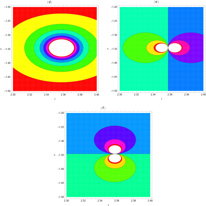

  

  Cone wave solution for the absolute, real, and imaginary parts of (9) in the contour plot

• Fig. 3 represents a dark wave solution of Eq. (21) when ($a_{3}=3$); $b_{1}=2$, $c=5$, $\eta=1$, $\kappa=0.5$, $\lambda=3$, $\mu =2$, $s=4$ in three distinct types of plots.

  Figure 3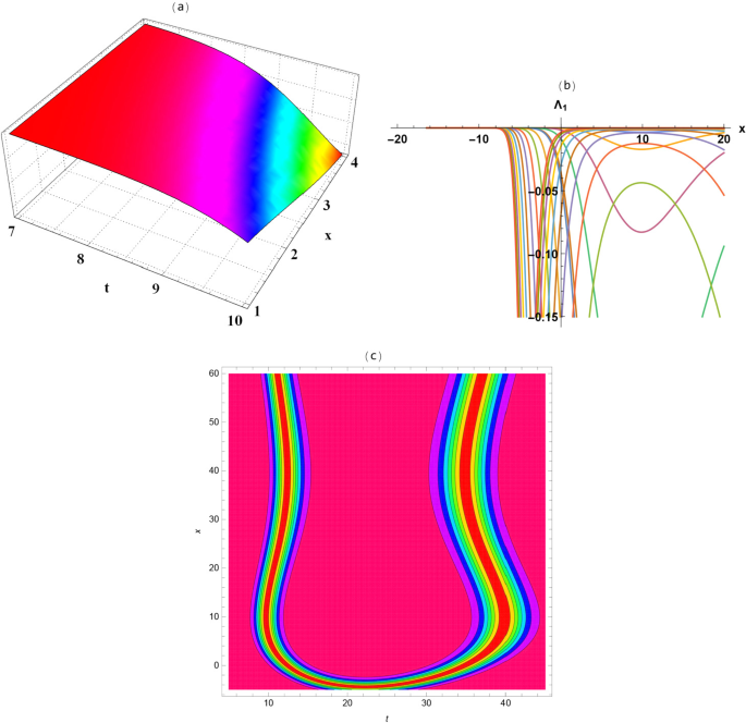

  

  Dark wave solution of (21) in three (a), two-dimensional (b), and contour plots (c)

• Fig. 4 shows dark wave solution of Eq. (23) when $a_{3}=3$, $b_{1}=2$, $c=5$, $\eta=1$, $\kappa=0.5$, $\lambda=3$, $\mu=2$, $s=4$ in three different plots.

  Figure 4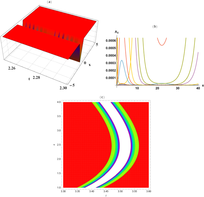

  

  Dark wave solution of (23) in three (a), two-dimensional (b), and contour plots (c)

• Fig. 5 shows dark wave solution of Eq. (34) when $a_{3}=3$, $b_{1}=2$, $c=5$, $\eta=1$, $\kappa=0.5$, $\lambda=3$, $\mu=0$, $s=4$ in three various kind of plots.

  Figure 5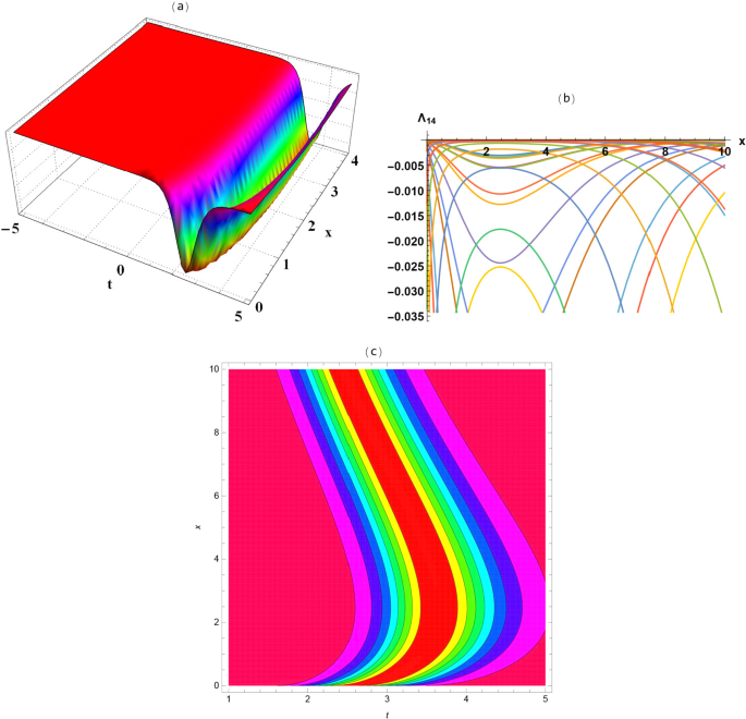

  

  Dark wave solution of (34) in three (a), two-dimensional (b), and contour plots (c)

• Fig. 6 shows bright wave solution of Eq. (35) when $c=3$, $h=2$, $\kappa=0.5$ in three different forms of sketches.

  Figure 6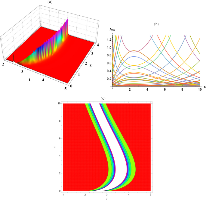

  

  Bright wave solution of (35) in three (a), two-dimensional (b), and contour plots (c)

4 Results and discussion

This segment displays our approaches and their latest functions. Check out how close we are and how the ideas we have found can be contrasted with the previously published papers. The key elements of our debate are the methodological approach employed and the approaches produced.

• 1. The computational schemes used:

  We used two computational methods (the extended exp-$( -\varphi (\vartheta) )$-expansion method and the Jacobi elliptical function method) for the fractional BP model and the EW model for constructing the exact traveling and solitary wave solutions. A compliant fractional operator was employed to transform fractional aspects of the equation to a nonlinear ordinary differential equation. This fractional operator enables the classification schemes to be extended to the transformed shape. All systems have the desired approach.

  $$\begin{aligned} \mathcal{H}(\vartheta) =&\Lambda(\vartheta) \\ =&\textstyle\begin{cases} \frac{\sum_{i=0}^{m} a_{i} e^{-i \phi(\vartheta)}}{\sum_{i=0}^{n} b_{i} e^{-i \phi(\vartheta)}}, \\ \quad \phi'(\vartheta) \to\lambda+\mu e^{\phi(\vartheta)}+\frac{1}{e^{\phi(\vartheta)}}, \\ \sum_{i=1}^{n} a_{i} \phi(\vartheta)^{i}+\sum_{i=1}^{n} b_{i} \phi (\vartheta)^{-i}+a_{0}, \\ \quad \phi'(\vartheta)\to\sqrt{p \phi(\vartheta )^{2}+q \phi(\vartheta)^{4}+\rho} , \end{cases}\displaystyle \end{aligned}$$

  (41)

  where $[n, m ]$ are arbitrary constants to be determined by using the homogeneous balance rule, while $[\lambda, \mu, p,q,\rho ]$ are arbitrary constants to be determined by solving the obtained algebraic system of equations. Moreover, applying two different schemes on one model shows its ability to be used for other various schemes where there is no unified method that is applied for all nonlinear evolution equations, and that is well demonstrated in our paper.

• 2. The obtained solutions:

  This part gives a comparison between our obtained solutions and those obtained in previously published papers. In [64], Mostafa M. A. Khater, Raghda A. M. Attia, and Dianchen Lu applied the modified Khater method to a fractional biological population model, fractional equal width model, and fractional modified equal width equation. They got many distinct types of solutions for these fractional biological models.

  • Eq. (27, [64]) is equal to Eq. (17) when [$\chi =2$, $\lambda=\nu$, $n \kappa=0$, $\varrho=\mu\sqrt{-\alpha\sigma}$].

  • All other obtained solutions of the fractional BP model are different from those obtained in [64].

  • All our obtained solutions of the fractional EW model are new and different from those obtained in [64].

5 Conclusion

This paper examined two nonlinear BP and EW fractional models via exp-$( -\varphi(\vartheta) )$-expansion and the Jacobi elliptical function method. The conformable fractional derivative has been employed to convert the nonlinear partial differential equations to an ordinary differential equation with an integer order. Many distinct wave solutions have been obtained and have been represented in three-, two-dimensional, and contour plots. These solutions were explained by different illustrations which clarify the new features of the fractional models in question. Our solutions have been explained in terms of precision and innovation. The novelty of our solutions is shown by comparing our solution with that obtained in previous research papers. The powerful and effective application of the used method is examined and tested to show its ability to be applied to other nonlinear evolution equations.

Appendix

Given function $f: [0,\infty)\rightarrow R$. Then the (conformable fractional derivative) of f of order α is defined by

$$\begin{aligned} T_{\alpha} (f) (t)=\lim_{\varepsilon\rightarrow0} \frac{f(t+\varepsilon t^{1-\alpha})-f(t)}{\varepsilon}. \end{aligned}$$

(42)

For all $t>0$, $\alpha\in(0,1)$ if f is α-differentiable in some $(0,\alpha)$. $\alpha>0$ and $\lim_{t\rightarrow0} f^{\alpha} (t)$ exists, then define $f^{\alpha}(0)=\lim_{t\rightarrow0} f^{\alpha}(t)$.

We sometimes write $f^{\alpha}(t)$ for $T_{\alpha}(f)(t)$ to denote the conformable fractional derivatives of f of order α. In addition, if the conformable fractional derivative of f of order α exists, then we say f is α-differentiable. We should take into consideration that $T_{\alpha}(t^{p})=p t^{p-\alpha}$. Further, this definition coincides with the same of traditional definition of Riemann–Liouville and of Caputo on polynomials (up to a constant multiple).

The conformable fractional properties:

• $T_{\alpha}(e^{c t})=c t^{1-\alpha} e^{c t}$.

• $T_{\alpha}(\sin(a t))=a t^{1-\alpha} \cos(a t)$.

• $T_{\alpha} \sin(a t)=-a t^{1-\alpha} \sin(a t)$.

• $T_{\alpha}(\tan(a t))=a t^{1-\alpha} \sec^{2}(a t)$.

• $T_{\alpha} (\cot(a t))=-a t^{1-\alpha} \csc^{2}(a t)$.

• $T_{\alpha} (\sec(a t))=a t^{1-\alpha} \sec(a t) \tan(a t)$.

• $T_{\alpha} (\csc(a t))=-a t^{1-\alpha} \csc(a t) \cot(a t)$.

• $T_{\alpha} ( \frac{t^{\alpha}}{\alpha} )=1$.

References

Khater, M.M.A., Attia, R.A.M., Abdel-Aty, A.-H., Abdel-Khalek, S., Al-Hadeethi, Y., Lu, D.: On the computational and numerical solutions of the transmission of nerve impulses of an excitable system (the neuron system). J. Intell. Fuzzy Syst. 38, 2603–2610 (2020)
Abdalla, M.S., Abdel-Aty, M., Obada, A.-S.F.: Degree of entanglement for anisotropic coupled oscillators interacting with a single atom. J. Opt. B, Quantum Semiclass. Opt. 4, 396–401 (2002)
Yang, X.-J., Tenreiro Machado, J.: A new fractal nonlinear Burgers’ equation arising in the acoustic signals propagation. Math. Methods Appl. Sci. 42(18), 7539–7544 (2019)
Janaki, M., Kanagarajan, K., Elsayed, E.M.: A note on nonlinear implicit neutral Katugampola fractional differential equations with impulse effects and finite delay. Sohag J. Math. 6(2), 29–39 (2019)
Alharbi, S.A., Rambely, A.S.: Dynamic behaviour and stabilisation to boost the immune system by complex interaction between tumour cells and vitamins intervention. Adv. Differ. Equ. 2020(1), 412 (2020)
Yang, X.-J.: General Fractional Derivatives: Theory, Methods and Applications, vol. 1. CRC Press, Boka Raton (2019)
Yang, X.-J., Feng, Y.-Y., Cattani, C., Inc, M.: Fundamental solutions of anomalous diffusion equations with the decay exponential kernel. Math. Methods Appl. Sci. 42(11), 4054–4060 (2019)
Rizvi, S.R., Afzal, I., Ali, K., Younis, M.: Stationary Solutions for Nonlinear Schrödinger Equations by Lie Group Analysis. Acta Phys. Pol. A 136, 187–189 (2019)
Khater, M.M.A., Attia, R.A.M., Abdel-Aty, A.: Computational analysis of a nonlinear fractional emerging telecommunication model with higher–order dispersive cubic–quintic. Inf. Sci. Lett. 9, 83–93 (2020)
Arif, A., Younis, M., Imran, M., Tantawy, M., Rizvi, S.T.R.: Solitons and lump wave solutions to the graphene thermophoretic motion system with a variable heat transmission. Eur. Phys. J. Plus 134(6), 303 (2019)
Liu, J.-G., Yang, X.-J., Feng, Y.-Y.: On integrability of the time fractional nonlinear heat conduction equation. J. Geom. Phys. 144, 190–198 (2019)
Wu, B., Sun, C.: Multiple positive solutions for a continuous fractional boundary value problem with fractional q-differences. Sohag J. Math. 7(2), 43–48 (2020)
Liang, Y., Yang, H., Li, H.: Existence of positive solutions for the fractional q-difference boundary value problem. Adv. Differ. Equ. 2020(1), 416 (2020)
Rizvi, S.T.R., Afzal, I., Ali, K.: Chirped optical solitons for Triki–Biswas equation. Mod. Phys. Lett. B 33(22), 1950264 (2019)
Liu, J.-G., Yang, X.-J., Feng, Y.-Y., Cui, P.: On group analysis of the time fractional extended \((2+ 1)\)-dimensional Zakharov–Kuznetsov equation in quantum magneto-plasmas. Math. Comput. Simul. 178, 407–421 (2020)
Alshammari, M., Al-Smadi, M., Alshammari, S., Abu Arqub, O., Hashim, I., Alias, M.: An attractive analytic-numeric approach for the solutions of uncertain Riccati differential equations using residual power series. Appl. Math. Inf. Sci. 14, 177–190 (2020)
Owyed, S., Abdou, M., Abdel-Aty, A.-H., Alharbi, W., Nekhili, R.: Numerical and approximate solutions for coupled time fractional nonlinear evolutions equations via reduced differential transform method. Chaos Solitons Fractals 131, 109474 (2020)
Jiang, Y., Ge, Y.: An explicit fourth-order compact difference scheme for solving the 2D wave equation. Adv. Differ. Equ. 2020(1), 415 (2020)
Lu, D., Seadawy, A.R., Khater, M.M.: Structures of exact and solitary optical solutions for the higher-order nonlinear Schrödinger equation and its applications in mono-mode optical fibers. Mod. Phys. Lett. B 33(23), 1950279 (2019)
Golmankhaneh, A.K., Tunc, C., Nia, S.M., Golmankhaneh, A.K.: A review on local and non-local fractal calculus. Numer. Comput. Methods Sci. Eng. 1, 19–31 (2019)
Khater, M.M., Lu, D., Attia, R.A.: Dispersive long wave of nonlinear fractional Wu–Zhang system via a modified auxiliary equation method. AIP Adv. 9(2), 025003 (2019)
Khater, M.M., Lu, D., Attia, R.A.: Erratum: “Dispersive long wave of nonlinear fractional Wu–Zhang system via a modified auxiliary equation method” [AIP Adv. 9, 025003 (2019)]. AIP Adv. 9(4), 049902 (2019)
Khater, M.M., Lu, D., Attia, R.A.: Lump soliton wave solutions for the \((2+ 1)\)-dimensional Konopelchenko–Dubrovsky equation and KdV equation. Mod. Phys. Lett. B 2019, 1950199 (2019)
Panda, S.K., Abdeljawad, T., Ravichandran, C.: Novel fixed point approach to Atangana-Baleanu fractional and LP-Fredholm integral equations. Alex. Eng. J. 59(4), 1959–1970 (2020)
Yang, S., Deng, M., Ren, R.: Stochastic resonance of fractional-order Langevin equation driven by periodic modulated noise with mass fluctuation. Adv. Differ. Equ. 2020(1), 1 (2020)
Liu, J.-G., Yang, X.-J., Feng, Y.-Y.: On integrability of the extended \((3+ 1)\)-dimensional Jimbo–Miwa equation. Math. Methods Appl. Sci. 43(4), 1646–1659 (2020)
Al-Refai, M., Pal, K.: New aspects of Caputo–Fabrizio fractional derivative. Prog. Fract. Differ. Appl. 5(2), 157–166 (2019)
Chatzarakis, G., Deepa, M., Nagajothi, N., Sadhasivam, V.: Oscillatory properties of a certain class of mixed fractional differential equations. Appl. Math. Inf. Sci. 14, 123–131 (2020)
Khater, M.M., Attia, R.A., Abdel-Aty, A.-H., Abdou, M., Eleuch, H., Lu, D.: Analytical and semi-analytical ample solutions of the higher-order nonlinear Schrödinger equation with the non-Kerr nonlinear term. Results Phys. 16, 103000 (2020)
Park, C., Khater, M.M.A., Abdel-Aty, A.-H., Attia, R.A.M., Rezazadeh, H., Zidan, A.M., Mohamed, A.-B.A.: Dynamical analysis of the nonlinear complex fractional emerging telecommunication model with higher–order dispersive cubic–quintic. Alex. Eng. J. 59(3), 1425–1433 (2020)
Cattani, C., Rushchitsky, J., Sinchilo, S.: Physical constants for one type of nonlinearly elastic fibrous micro-and nanocomposites with hard and soft nonlinearities. Int. Appl. Mech. 41(12), 1368–1377 (2005)
Singh, J., Kumar, D., Hammouch, Z., Atangana, A.: A fractional epidemiological model for computer viruses pertaining to a new fractional derivative. Appl. Math. Comput. 316, 504–515 (2018)
Cattani, C., Pierro, G.: On the fractal geometry of DNA by the binary image analysis. Bull. Math. Biol. 75(9), 1544–1570 (2013)
Zhang, J.-G.: The Fourier–Yang integral transform for solving the 1-D heat diffusion equation. Therm. Sci. 21(1), 63–69 (2017)
Liu, J.-G., Yang, X.-J., Feng, Y.-Y., Zhang, H.-Y.: Analysis of the time fractional nonlinear diffusion equation from diffusion process. J. Appl. Anal. Comput. 10, 1060–1072 (2020)
Hasanov, A., Choi, J.: Note on Euler–Bernoulli equation. Sohag J. Math. 7(2), 33–36 (2020)
Babaei, A., Jafari, H., Liya, A.: Mathematical models of HIV/AIDS and drug addiction in prisons. Eur. Phys. J. Plus 135(5), 395 (2020)
Wang, S., Li, Y., Shao, Y., Cattani, C., Zhang, Y., Du, S.: Detection of dendritic spines using wavelet packet entropy and fuzzy support vector machine. CNS Neurol. Disord. Drug Targets 16(2), 116–121 (2017)
Widyan, A.M.: Chance constrained approach for treating multicriterion inventory model with random variables in the constraints. J. Stat. Appl. Pro. 9(2), 207–213 (2020)
Kanth, A.R., Garg, N.: Computational simulations for solving a class of fractional models via Caputo–Fabrizio fractional derivative. Proc. Comput. Sci. 125, 476–482 (2018)
Du, Q., Hesthaven, J.S., Li, C., Shu, C.-W., Tang, T.: Preface to the Focused Issue on Fractional Derivatives and General Nonlocal Models. Commun. Appl. Math. Comput. Sci. 1(4), 503–504 (2019)
Abdelhakem, M., Ahmed, A., El-kady, M.: Spectral monic Chebyshev approximation for higher order differential equations. Math. Sci. Lett. 8, 11–17 (2019)
Giusti, A.: A comment on some new definitions of fractional derivative. Nonlinear Dyn. 93(3), 1757–1763 (2018)
Al-Saif, A.S.J., Abdul-Wahab, M.S.: Application of new simulation scheme for the nonlinear biological population model. Numer. Comput. Methods Sci. Eng. 1, 89–99 (2019)
Abdeljawad, T., Al-Mdallal, Q.M., Jarad, F.: Fractional logistic models in the frame of fractional operators generated by conformable derivatives. Chaos Solitons Fractals 119, 94–101 (2019)
Martinez, L., Rosales, J., Carreño, C., Lozano, J.: Electrical circuits described by fractional conformable derivative. Int. J. Circuit Theory Appl. 46(5), 1091–1100 (2018)
Nchama, G.A.M., Mecıas, A.L., Richard, M.R.: The Caputo–Fabrizio fractional integral to generate some new inequalities. Inf. Sci. Lett. 8, 73–80 (2019)
Shakeel, M., Iqbal, M.A., Mohyud-Din, S.T.: Closed form solutions for nonlinear biological population model. J. Biol. Syst. 26(01), 207–223 (2018)
Bushnaq, S., Ali, S., Shah, K., Arif, M.: Exact solution to non-linear biological population model with fractional order. Therm. Sci. 22(1), 317–327 (2018)
Xu, Y., Lu, D.: Study on Approximate Solution of Fractional Order Biological Population Model. Arch. Curr. Res. Int. 15, 1–11 (2018)
Wu, C., Rui, W.: Method of separation variables combined with homogenous balanced principle for searching exact solutions of nonlinear time-fractional biological population model. Commun. Nonlinear Sci. Numer. Simul. 63, 88–100 (2018)
Goswami, A., Singh, J., Kumar, D., et al.: An efficient analytical approach for fractional equal width equations describing hydro–magnetic waves in cold plasma. Phys. A, Stat. Mech. Appl. 524, 563–575 (2019)
Zafar, A.: Rational exponential solutions of conformable space–time fractional equal-width equations. Nonlinear Eng. 8(1), 350–355 (2019)
Hassan, S., Abdelrahman, M.A.: Solitary wave solutions for some nonlinear time–fractional partial differential equations. Pramana 91(5), 67 (2018)
Ray, S.S.: Invariant analysis and conservation laws for the time fractional \((2+ 1)\)-dimensional Zakharov–Kuznetsov modified equal width equation using Lie group analysis. Comput. Math. Appl. 76(9), 2110–2118 (2018)
Baskonus, H.M., Bulut, H., Atangana, A.: On the complex and hyperbolic structures of the longitudinal wave equation in a magneto–electro–elastic circular rod. Smart Mater. Struct. 25(3), 035022 (2016)
Koçak, Z.F., Bulut, H., Koc, D.A., Baskonus, H.M.: Prototype traveling wave solutions of new coupled Konno–Oono equation. Optik 127(22), 10786–10794 (2016)
Baskonus, H.M., Bulut, H., Belgacem, F.B.M.: Analytical solutions for nonlinear long–short wave interaction systems with highly complex structure. J. Comput. Appl. Math. 312, 257–266 (2017)
Hafez, M., Akbar, M.: An exponential expansion method and its application to the strain wave equation in microstructured solids. Ain Shams Eng. J. 6(2), 683–690 (2015)
Ayatollahi, M., Safavi-Naeini, S.: A fast analysis method based on exponential expansion of Green’s function for large multilayer structures. In: IEEE Antennas and Propagation Society International Symposium. 2001 Digest. Held in Conjunction with: USNC/URSI National Radio Science Meeting (Cat. No. 01CH37229), vol. 4, pp. 850–853 (2001)
Tala-Tebue, E., Djoufack, Z., Fendzi-Donfack, E., Kenfack-Jiotsa, A., Kofané, T.: Exact solutions of the unstable nonlinear Schrödinger equation with the new Jacobi elliptic function rational expansion method and the exponential rational function method. Optik 127(23), 11124–11130 (2016)
Tasbozan, O., Çenesiz, Y., Kurt, A.: New solutions for conformable fractional Boussinesq and combined KdV–mKdV equations using Jacobi elliptic function expansion method. Eur. Phys. J. Plus 131(7), 244 (2016)
Feng, Q., Meng, F.: Traveling wave solutions for fractional partial differential equations arising in mathematical physics by an improved fractional Jacobi elliptic equation method. Math. Methods Appl. Sci. 40(10), 3676–3686 (2017)
Khater, M., Attia, R., Lu, D.: Modified Auxiliary Equation Method versus Three Nonlinear Fractional Biological Models in Present Explicit Wave Solutions. Math. Comput. Appl. 24(1), 1 (2019)
Acknowledgements
This project was funded by the Deanship of Scientific Research (DSR), King Abdulaziz University, Jeddah, under grant No. (D-671-305-1441). The authors, therefore, gratefully acknowledge DSR technical and financial support.
Availability of data and materials
Not applicable.
Funding
Author information
Authors and Affiliations
Contributions
All authors conceived of the study, participated in its design and coordination, drafted the manuscript, participated in the sequence alignment, and read and approved the final manuscript.
Corresponding author
Ethics declarations
Competing interests
The authors declare that they have no competing interests.