Supplier risk assessment based on trapezoidal intuitionistic fuzzy numbers and ELECTRE TRI-C: a case illustration involving service suppliers

Abstract

Many companies today have embraced the concept of risk management, usually in the form of enterprise risk management or supply chain risk management. Both are based on a holistic view of risks. Hence, risks related to specific functions within a company must be considered more broadly than previously. Risks, however, involve uncertainty, and the less specific the context in which risks are viewed, the more uncertainty will be involved. One particular way to express uncertainty is through trapezoidal intuitionistic fuzzy numbers (TrIFNs). In this paper, risks that are relevant for supplier risk assessments are first collected from the literature. Then it is illustrated how the multi-criteria decision analysis method ELECTRE TRI-C can be used for sorting suppliers into risk categories, when the risks as well as some of the method’s parameters are expressed with TrIFNs. In order to do this, we make use of a small modification of an existing method for converting TrIFNs into crisp values. The approach is illustrated in a case problem based on a company that is looking for service providers (suppliers) of electrical maintenance. The problem involves 20 suppliers that are sorted into three risk categories based on evaluations from 27 criteria. Results from the case study point to two low risk suppliers. A further ad-hoc analysis suggests one of these to be less risky than the other.

Appendices

Appendix A

A.1. Decision matrix

An MCDA problem generally include a set of alternatives or actions A={a _i :i=1, 2, …, n}, which has to be evaluated on a set of criteria F={g _j :j=1, 2, …, m}. It is common to denote an evaluation or performance of alternative a _i on criterion g _j as g _j (a _i ), where g _j ( ⋅ ) is a criterion function corresponding to the scale and the possible values of evaluations on criterion g _j .

A decision matrix M _{n × m} with n rows and m columns is defined as:

Note that in standard matrix notation m is used to indicate the number of rows and n to indicate the number of columns. In MCDA problems, it is customary to use n and m to indicate the number of alternatives, respectively, criteria. Since we prefer to present alternatives in rows, we use n rows and m columns.

When analysing an MCDA problem, we need to know the direction of preferences on each criterion, i.e. if a high or a low value of g _j (a _i ) is preferred. Criteria of the former type are referred to as benefit criteria and criteria of the latter type as cost criteria.

A.2. Criteria weights

Many MCDA methods require that each criterion be given a weight, in order to indicate the relative importance of the criteria. These weights are interpreted differently in various MCDA methods (Choo et al, 1999). In ELECTRE methods, each weight is interpreted as the voting power of the corresponding criterion in a coalition in favour of an outranking (Figueira et al, 2005).

Several methods have been proposed to aid a DM in determining criteria weights (Choo et al, 1999). Some applications of such methods can be found in Massam (1991) (AHP), Milani and Shanian (2006) (Entropy method), Certa et al (2009) (ANP), and Zardari et al (2010) (Conjoint analysis). Specifically aimed at ELECTRE, Rogers and Bruen (1998) proposed the ‘resistance to change grid’, Figueira and Roy (2002) presented the revised Simos’ card procedure, and Greco et al (2002) proposed to use decision rules obtained by a dominance-based rough set approach. For ELECTRE TRI, a number of preference disaggregation procedures have been developed (see Govindan and Jepsen, 2015).

We denote a set of criteria weights as {k _j |k _j >0, ∀j∈J}.

A.3. Discrimination thresholds and types of criteria

The most general form of criteria used in ELECTRE methods are pseudo-criteria. A pseudo-criterion takes into account the imperfect nature of a DM’s evaluations of the alternatives. For a pseudo-criterion g _j ∈F, two threshold functions must be defined (Figueira et al, 2010):

• Indifference threshold q _j ( ⋅ )

• Preference threshold p _j ( ⋅ )

These two thresholds are generally referred to as discrimination thresholds. An indifference threshold indicates a zone, in which the difference of the evaluations of two alternatives does not justify a preference of one over the other. The preference threshold, on the other hand, indicates a level, such that in order for an alternative a to be regarded as better than alternative a′, the difference g _j (a)−g _j (a′) of the evaluations must exceed the given threshold level. If the difference lies in a zone between the indifference threshold and the preference threshold, then a hesitation between indifference and preference occurs (Figueira et al, 2005).

The threshold functions must satisfy the condition p _j (g _j (a))⩾q _j (g _j (a))⩾0 for all a∈A. They can either be constant or vary according to the evaluations. If a threshold is variable, then a distinction is made between a direct threshold and an inverse threshold, corresponding to whether the threshold is computed using the best or the worst evaluation, respectively, whenever two alternatives are under consideration (Figueira et al, 2010).

When using variable thresholds, further restrictions apply to the parameters of the functions. Usually the threshold functions are given as affine functions. In such a case, the function of a direct indifference threshold can be expressed⁹ as , where , such that α _qj >−1 on a benefit criterion and on a cost criterion. An inverse threshold is expressed as , where , such that on a benefit criterion and on a cost criterion. For preference thresholds, simply exchange q with p everywhere. If a threshold function is defined as direct (inverse), then the parameters necessary for the function for the inverse (direct) threshold can be obtained through a transformation, because direct and inverse thresholds are functionally linked. Note that when using variable thresholds in ELECTRE TRI, TRI-C, and TRI-nC, the threshold functions are based on the performance of a reference norm. These methods are created, such that the algorithm takes care of the transformations, because separate formulas are used if an alternative is compared to a norm or if a norm is compared to an alternative. In other ELECTRE methods with pseudo-criteria, the formulas are based on input in the form of direct thresholds; hence, if inverse thresholds are preferred, then the parameters must be transformed. For more details on variable thresholds, please refer to Dias (2011). In this paper, we only consider input in the form of constant thresholds.

Let p _j (a′) and q _j (a′) be the thresholds associated with criterion g _j ∈F and a particular alternative a′∈A. Then a pseudo-criterion g _j reduces to (Roy, 1996):

• A true criterion, if p _j (a)=q _j (a)=0 for all a∈A

• A semi-criterion, if p _j (a)=q _j (a) for all a∈A

• A pre-criterion, if q _j (a)=0 for all a∈A

In ELECTRE I and II (and the unofficial ELECTRE IV), only true criteria are used, whereas the other ELECTRE methods are based on pseudo-criteria. Any single criterion in the latter methods can still be reduced to any of the other types of criteria though.

A.4. Veto thresholds

A veto threshold v _j ( ⋅ ) can be assigned to each criterion. In the case of pseudo-criteria, it can be either constant or a function of the performances. As was the case for the discrimination thresholds, a further distinction is made between a direct and an inverse threshold if the threshold is variable. Generally, it must satisfy the condition v _j (g _j (a))⩾p _j (g _j (a)) for all a∈A and if variable thresholds are used, similar restrictions apply as the ones mentioned in Section A.3 for the indifference and preference thresholds. In the method referred to as ELECTRE IV and in applications, where veto thresholds are used in ELECTRE I and II, the thresholds are usually constant. In this paper, we only consider input in the form of constant thresholds.

A veto threshold indicates the maximum difference allowed between the performances of two alternatives on a specific criterion. A single veto threshold can invalidate an outranking regardless of what the other performances are, if the difference between two performances on a given criterion exceeds the veto thresholds (Roy, 1991).

A.5. Concordance, discordance, and credibility indices used in some ELECTRE methods

The formulas in the following subsections are used in ELECTRE III, TRI, TRI-C, and TRI-nC. The concordance formula is also used in ELECTRE IS.

A.5.1. Concordance indices

A concordance index c(x, y) for an ordered pair (x, y) is given as follows:

where c _j (x, y) is the jth partial concordance index for (x, y) and given as follows:

For a benefit criterion:

The formula for c _j (x, y) on a benefit criterion can be generalized to:

For a cost criterion:

The formula for c _j (x,y) on a cost criterion can be generalized to:

A.5.2. Partial discordance indices

A partial concordance index d _j (x, y) for an ordered pair (x, y) is given as follows:

For a benefit criterion

The formula above can be generalized to:

For a cost criterion

The formula above can be generalized to:

A.5.3. Credibility indices

A credibility index σ(x, y) for an ordered pair (x, y) is given as follows:

where

A.6. ELECTRE TRI-C

ELECTRE TRI-C was designed for the sorting problematic, but instead of using limits (profiles) to determine the categories as in ELECTRE TRI, a characteristic action must be defined for each category. A characteristic action indicates the typical performance on each criterion g _j ∈F of an action (alternative) in the corresponding category. Apart from these characteristic actions, an additional parameter, called a credibility level, needs to be determined. It is similar to the cutting level in ELECTRE TRI, but has an additional restriction. In ELECTRE TRI-C, the exploitation phase includes two assignment rules as in ELECTRE TRI, but they must be considered jointly. Hence, if the two rules do not assign a particular alternative to the same category, then the two different categories define a range of possible categories for the final assignment of the alternative.

A stepwise illustration is provided in the following sub-section. The illustration is based on the description in Dias et al (2010). Note that the notation in the illustration is based on constant thresholds. For variable thresholds, simply exchange the constant threshold with the expression for the variable threshold.

A.6.1. Stepwise illustration of ELECTRE TRI-C

The stepwise illustration below is based on the description in Dias et al (2010). Note that we interchangeably use the terms action and alternative in the illustration.

Step 1::

Create a decision matrix M and assign a weight k _j to each criterion g _j ∈F.

Step 2::

Determine indifference and preference thresholds q _j and p _j for each criterion g _j ∈F, such that p _j ⩾q _j (see section A.3).

Step 3::

For any criterion g _j ∈F, a veto threshold v _j ⩾p _j can be determined if desired (see Section A.4)

Step 4::

In this step, a set of ordered categories must be defined. For this purpose, a set of characteristic actions b _h , h=1, …, q must be defined, where q is the number of desired categories. Let g _j (b _h ) denote the performance value of b _h on criterion g _j and {C _h } _h =₁, …, _q the set of categories. A characteristic action b _h must be defined, such that g _j (b _h ) is a typical performance value on criterion g _j for an alternative assigned to category C _h .

In what follows, let:

• F ⁺={g _j ∈F|g _j is a benefit criterion}

• F ⁻={g _j ∈F|g _j is a cost criterion}

The characteristic actions must as a minimum fulfil the following conditions:

• g _j (b _h+1)⩾g _j (b _h ) for h=1, …, q−1 and for all g _j ∈F ⁺

• g _j (b _h+1)⩽g _j (b _h ) for h=1, …, q−1 and for all g _j ∈F ⁻

• At least one of the following two conditions is true:

  • ° There is at least one g _j ∈F ⁺, such that g _j (b _h+1)>g _j (b _h ) for h=1, …, q−1

  • ° There is at least one g _j ∈F ⁻, such that g _j (b _h+1)<g _j (b _h ) for h=1, …, q−1

• The set {b _h |h=1, …, q} of characteristic actions fulfills the weak separability condition (see Section A.6.2)

In addition, any of the two stronger conditions strict separability or hyper-strict separability can be applied (see Section A.6.2). The stronger the condition the set of characteristic actions fulfills, the better the categories can be distinguished by the ELECTRE TRI-C method.

Finally, two special characteristic actions b ₀ and b _q+1 must be defined, such that:

• g _j (b ₀)<g _j (a)<g _j (b _q+1) for all g _j ∈F ⁺, a∈A

• g _j (b ₀)>g _j (a)>g _j (b _q+1) for all g _j ∈F ⁻, a∈A

• g _j (b ₁)−g _j (b ₀)>0 for all g _j ∈F ⁺

• g _j (b ₀)−g _j (b ₁)>0 for all g _j ∈F ⁻

• g _j (b _q+1)−g _j (b _q )>0 for all g _j ∈F ⁺

• g _j (b _q )−g _j (b _q+1)>0 for all g _j ∈F ⁻

That is, the two special characteristic actions represents the worst and the best possible performance, respectively, of an alternative on the specific criterion.

Let B={b _h |h=0, …, q+1}.

Step 5::

Compute a concordance index c(a, b _h ) for any pair (a, b _h ), a∈A, b _h ∈B. See section A.5.1 for formulas.

Step 6::

Compute a concordance index c(b _h , a) for any pair (a, b _h ), a∈A, b _h ∈B. See Section A.5.1 for formulas.

Step 7::

Compute partial discordance indices d _j (a _i , b _h ) for any pair (b _h , a), a∈A, b _h ∈B. See section A.5.2 for formulas.

Step 8::

Compute partial discordance indices d _j (b _h , a) for any pair (b _h , a), a∈A, b _h ∈B. See Section A.5.2 for formulas.

Step 9::

Compute a credibility index σ _j (a, b _h ) for any pair (a, b _h ), a∈A, b _h ∈B. See Section A.5.3 for formulas.

Step 10::

Compute a credibility index σ _j (b _h , a) for any pair (b _h , a), a∈A, b _h ∈B. See Section A.5.3 for formulas.

Step 11::

Determine a minimum credibility level λ, 1/2⩽λ⩽1, such that

λ⩾max{σ(b _h , b _h+1)∣h=1, …, q−1}.

The credibility level is the minimum degree of credibility considered necessary to validate an outranking of one action over another. It should, in general, be within the range [0.5, 1]. If, however, the set of characteristic actions only fulfills the weak separability condition, then the minimum required credibility level is further restricted by the maximum of credibility indices σ(b _h , b _h+1), h=1, 2, …,q−1, such that in addition to the restriction λ∈[0.5, 1], also max{σ(b _h , b _h+1)∣h=1, 2, …, q−1}⩽λ⩽1 must be fulfilled (Dias et al, 2010).

Step 12::

As is the case for ELECTRE TRI, ELECTRE TRI-C uses two assignment (exploitation) procedures. In ELECTRE TRI-C, however, the resulting assignments should be considered jointly. That is, if the two procedures suggest different categories for an alternative to be placed in, then the two categories define a range of possible categories for the alternative under consideration.

Before the two procedures are illustrated in Steps 13–15, we need to define the possible preference situations between a∈A and b _h ∈B. Let aP ⁺ b _h , denote a preference of a over b _h and let aP ⁻ b _h denote the situation b _h P ⁺ a. For the two special characteristic actions b ₀ and b _q+1, it is always the case that aP ⁺ b ₀ and aP ⁻ b _q+1. Indifference is indicated as aIb _h and incomparability as aRb _h .

The preference situations between a∈A and b _h ∈B are defined as follows:

• If σ(a, b _h )⩾λ and σ(b _h , a)⩾λ, then aIb _h .

• If σ(a, b _h )⩾λ and σ(b _h , a)<λ, then aP ⁺ b _h .

• If σ(a, b _h )<λ and σ(b _h , a)⩾λ, then aP ⁻ b _h .

• If σ(a, b _h )<λ and σ(b _h , a)<λ, then aRb _h .

Note that Dias et al (2010) use the notation aI ^λ b _h (λ-indifference), aP ^λ b _h (λ-preference of a _i over b _h ) and aR ^λ b _h (λ-incomparability).

Step 13::

For the two assignment procedures, it is necessary to define a selecting function ρ, which is used to select between two consecutive categories for the assignment of an alternative in each of the procedures in Steps 14–15. Dias et al (2010) define a number of properties, the selecting function should have, and propose the use of the min selecting function defined as:

Step 14::

Apply the first assignment procedure called the descending rule.

Dias et al (2010) describe the descending rule as follows:

• Decrease h from q+1 until the first value t, such that σ(a, b _t )⩾λ

  • If t=q, select C _q as a possible category for a

  • For 0<t<q, if ρ(a, b _t )<ρ(a, b _t+1), then select C _t as a possible category for a, otherwise select C _t+1

  • If t=0, select C ₁ as a possible category for a

Step 15::

Apply the second assignment procedure called the ascending rule.

Dias et al (2010) describe the ascending rule as follows:

• Increase h from zero until the first value t, such that σ(b _t , a)⩾λ

  • ° If t=1, select C ₁ as a possible category for a

  • ° For 1<t<q+1, if ρ(a, b _t )>ρ(a, b _t+1), then select C _t as a possible category for a, otherwise select C _t−1

  • ° If t=q+1, select C _q as a possible category for a

Step 16::

For each alternative a∈A, define the range of possible categories based on the minimum and maximum categories selected in Steps 14–15.

A.6.2. Separability conditions on characteristic actions

In order to test the weak, strict and/or hyper-strict separability conditions on the set of characteristic actions {b _h |h=1, …, q}, we have to go through the procedure of calculating concordance, discordance, and credibility indices for pairs of characteristic actions (b _k , b _k+1), k=1, …, q−1.

Step 1::

Determine concordance indices c _j (b _h , b _h+1), h=1, …, q−1, j=1, …, m. See Section A.5.1 for formulas.

Step 2::

Determine partial discordance indices d _j (b _h , b _h+1), h=1, …, q−1, j=1, …, m. See Section A.5.2 for formulas.

Step 3::

Determine credibility indices σ(b _h , b _h+1), h=1, …, q−1. See Section A.5.3 for formulas.

Step 4::

If σ(b _h , b _h+1)<1 for h=1, …, q−1, then the set of characteristic actions {b _h |h=1, …, q}fulfills the weak separability condition.

Step 5::

If σ(b _h , b _h+1)<1/2 for h=1, …, q−1, then the set of characteristic actions {b _h |h=1, …, q} also fulfills the strict separability condition.

Step 6::

If σ(b _h , b _h+1)=0 for h=1, …, q−1, then the set of characteristic actions {b _h |h=1, …, q} also fulfills the hyper-strict separability condition.

Appendix B

Appendix B Intuitionistic fuzzy numbers

In this appendix, we go through some of the definitions necessary for our use of intuitionistic fuzzy numbers.

Definition 1

• (Xu and Cai, 2012): Let X be a fixed set. An intuitionistic fuzzy set is a set

  

  where μ _A is referred to as a membership function and is defined as the mapping,

  

  and v _A is referred to as the non-membership function and is defined as the mapping

  

  such that

  

  The numerical values of μ _A (x) and ν _A (x) are called the membership degree and the non-membership degree of the element x∈X in A, respectively.

  If A is an IFS in X, then the value of

  

  is called the indeterminacy (or hesitancy) degree of the element x∈X to A.

  If ν _A (x)=1−μ _A (x) for all x∈X, then A degenerates into a fuzzy set.

Definition 2

• (Li, 2014): Let w _c ∈[0, 1] and u _c ∈[0, 1] be a pair of real numbers, such that 0⩽w _c +u _c ⩽1. An intuitionistic fuzzy number c is a special intuitionistic fuzzy set on the set of real numbers , where the membership function μ _c →[0, w _c ] and the non-membership function ν _c →[u _c , 1] satisfy the following four conditions (1)–(4):

  • 1) There exist at least two real numbers , such that μ _c (x′)=w _c and ν _c (x′)=u _c

  • 2) μ _c is quasi-concave and upper semi-continuous on

  • 3) ν _c is quasi-convex and lower semi-continuous on

  • 4) The support of c is compact. Note that the support of c is the set

  The numbers w _c and u _c are called the maximum membership degree and the minimum non-membership degree, respectively.

  A general intuitionistic fuzzy number is defined by the membership function

  

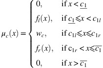
  and the non-membership function

  

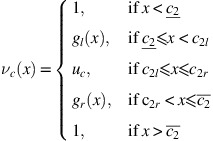
  where the functions and are continuous and non-decreasing, and satisfy the conditions , f _l (c _1l )=w _c , g _r (c _2r )=u _c , and the functions and are continuous and non-increasing and satisfy the conditions f _r (c _1r )=w _c , , , g _r (c _2l )=u _c .

  When , c _1l =c _2l , c _1r =c _2r and , we use the notation c=〈(c ₁, c ₂, c ₃, c ₄), w _c , u _c 〉 .

Definition 3

• (Li, 2014): Let , such that a ₁<a ₂<a ₃<a ₄. A trapezoidal intuitionistic fuzzy number (TrIFN) a=〈(a ₁, a ₂, a ₃, a ₄), w _a , u _a 〉 is defined by the membership function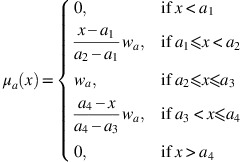

  

  and the non-membership function

  

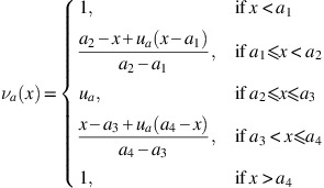
  Figure B1 illustrates a TrIFN.

  Figure B1

  

  Trapezoidal intuitionistic fuzzy number.

  If a ₁<a ₂=a ₃<a ₄, then the TrIFN degenerates into a triangular intuitionistic fuzzy number (TIFN). The same formulas can be used for membership and non-membership functions if a ₂⩽x⩽a ₃ is replaced with a ₂=x=a ₃. Figure B2 illustrates a triangular intuitionistic fuzzy number.

  Figure B2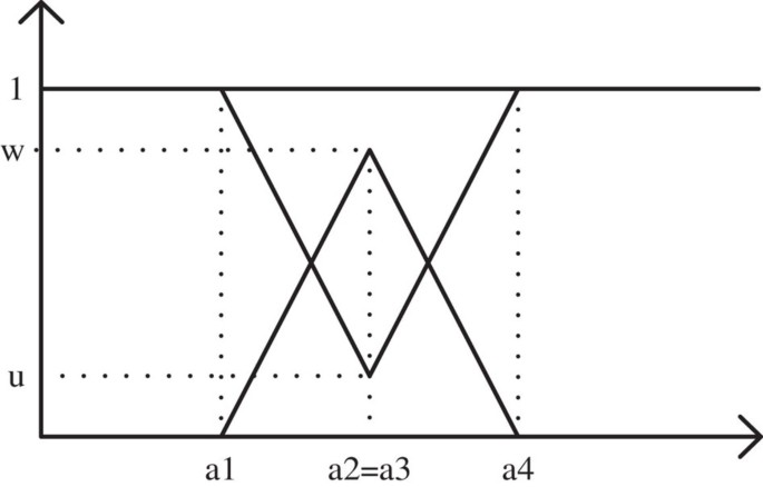

  

  Triangular intuitionistic fuzzy number.

  There are some other degenerate cases, which are not intuitionistic fuzzy numbers according to Definition 2. Nevertheless, they may be relevant in cases, where TrIFNs are used in real decision problems. For convenience, we use the notion of an intuitionistic fuzzy number also in these cases. Hence, in Definition 4, the membership and non-membership functions of what we refer to, as intuitionistic fuzzy numbers, do not fulfil all the conditions in Definition 2.

Definition 4

• We add the following definitions:

  • Case 1: If a ₁=a ₂<a ₃=a ₄ then we say that a=〈(a ₁,a ₂, a ₃, a ₄), w _a , u _a 〉 is an intuitionistic fuzzy interval number. Figure B3 illustrates the case.

    Figure B3

    

    Illustration of Case 1.

  • Case 2: If a ₁=a ₂=a ₃=a ₄ then we say that a=〈(a ₁, a ₂, a ₃, a ₄), w _a , u _a 〉 is an intuitionistic crisp number. Figure B4 illustrates the case. Note that each of the two small squares are endpoint of the two lines.

    Figure B4

    

    Illustration of Case 2.

  • Case 3: If a ₁=a ₂<a ₃<a ₄, then we say that a=〈(a ₁, a ₂, a ₃, a ₄), w _a , u _a 〉 is a right TrIFN. Figure B5 illustrates the case.

    Figure B5

    

    Illustration of Case 3

  • Case 4: If a ₁<a ₂<a ₃=a ₄, then we say that a=〈(a ₁, a ₂, a ₃, a ₄), w _a , u _a 〉 is a left TrIFN. Figure B6 illustrates the case.

    Figure B6

    

    Illustration of Case 4.

  • Case 5: If a ₁=a ₂=a ₃<a ₄, then we say that a=〈(a ₁, a ₂, a ₃, a ₄), w _a , u _a 〉 is a right triangular intuitionistic fuzzy number. Figure B7 illustrates the case.

    Figure B7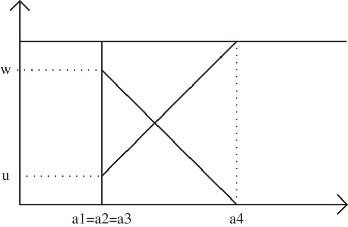

    

    Illustration of Case 5.

  • Case 6: If a ₁<a ₂=a ₃=a ₄, then we say that a=〈(a ₁, a ₂, a ₃, a ₄), w _a , u _a 〉 is a left triangular intuitionistic fuzzy number. Figure B8 illustrates the case.

    Figure B8

    

    Illustration of Case 6.

Definition 5

• (Li, 2014): Let a be an intuitionistic fuzzy number as in Definition 2 and let , such that 0⩽α⩽w _a and u _a ⩽β⩽1.

  An α-cut set of a is defined as the set a ^α={x∣μ(x)⩾α, x∈}, which can be represented by a closed interval denoted as [L _a (α), R _a (α)].

  A β-cut set of a is defined as the set , which can be represented by a closed interval denoted as [L _a (β), R _a (β)].

Definition 6

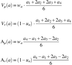
• (Li, 2014): Let a be an intuitionistic fuzzy number as in Definition 2 and let , such that 0⩽α⩽w _a and u _a ⩽β⩽1.

  The value indices (or values for short) of the membership and the non-membership are defined as

  

  The ambiguity indices (or ambiguities for short) of the membership and the non-membership are defined as

  

  where f:[0, w _c ]→[0, 1] is monotonic and non-decreasing and satisfy the condition f(0)=0, and g:[u _c , 1]→[0, 1] is monotonic and non-increasing and satisfy the condition g(1)=0.

  The value indices are related to the concept of centroids of the membership and non-membership functions and the ambiguity indices can be seen as the global spreads of the membership and non-membership functions (Li, 2014).

Definition 7

• (Li, 2014): Let a be an intuitionistic fuzzy number as in Definition 2 and let V _μ (a), V _ν (a), A _μ (a) and A _ν (a) be the value indices and ambiguity indices of a. Moreover, let 0⩽λ⩽1.

  The λ-weighted value index V _λ (a) and the λ-weighted ambiguity index A _λ (a) of a are defined as

  

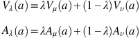
  The parameter λ can be used to indicate preferences between the values of the membership and non-membership functions. This can also be seen as a preference between certainty and uncertainty. Hence, if λ<1/2, then uncertainty is preferred, if λ>1/2, then certainty is preferred and if λ=1/2, then certainty and uncertainty are equally preferred. For this paper, we let λ=0.5.

  The ranking of two intuitionistic fuzzy numbers a and b can be determined using λ-weighted values and λ-weighted ambiguities as follows:

  • if V _λ (a)>V _λ (b) then a>b

  • if V _λ (a)<V _λ (b) then a<b

  • if V _λ (a)=V _λ (b)∧A _λ (a)<A _λ (b) then a>b

  • if V _λ (a)=V _λ (b)∧A _λ (a)>A _λ (b) then b>a

  • if V _λ (a)=V _λ (b)∧A _λ (a)=A _λ (b) then a=b

Definition 8

• (Li, 2014): Let a=〈(a ₁, a ₂, a ₃, a ₄), w _a , u _a 〉 be a TrIFN and let , such that 0⩽α⩽w _a and u _a ⩽β⩽1. Then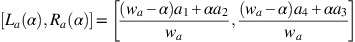

  

  and

  

  If a is a TIFN with a ₁<a ₂=a ₃<a ₄, then the formulas can also be applied.

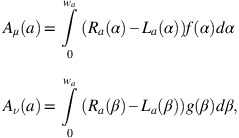
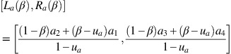
Definition 9

• Let a=〈(a ₁, a ₂, a ₃, a ₄), w _a , u _a 〉 be a TrIFN and let 0⩽α⩽w _a and u _a ⩽β⩽1. Moreover, let f(α)=α/w _a and g(β)=(1−β)/(1−u _a ). Then

  
  
  
  

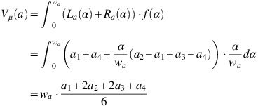
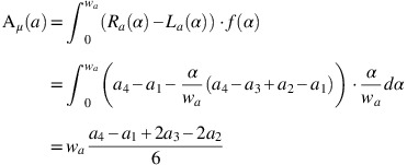
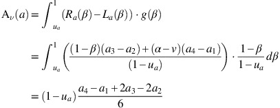
  Note that if a is a TIFN with a ₁<a ₂=a ₃<a ₄, then it can be shown that the formulas also hold. For this paper, value and ambiguity indices will be based on the formulas from Definition 9.

Definition 10

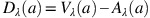
• (Li and Yang, 2013): Let a=〈(a ₁, a ₂, a ₃, a ₄),w _a , u _a 〉 be a TrIFN and let 0⩽α⩽w _a and u _a ⩽β⩽1. Moreover, let V _λ (a) and A _λ (a) be the corresponding λ-weighted value and ambiguity index as in Definition 7. Then the λ-weighted difference index D _λ (a) is defined as

  

  The ranking of two intuitionistic fuzzy numbers a and b is determined using λ-weighted difference indices as follows:

  • if D _λ (a)>D _λ (b) then a>b

  • if D _λ (a)<D _λ (b) then a<b

  • if D _λ (a)=D _λ (b) then a=b

Definition 11

• If a=〈(a ₁, a ₂, a ₃, a ₄), w _a , u _a 〉 is one of the degenerate intuitionistic fuzzy numbers from Definition 4, then we define

  

  and

  

  and

  

Appendix C:

Data for the case study

Table C1

Table C1 Fuzzy decision matrix

Table C2

Table C2 Fuzzy characteristic actions

References

Adhitya A, Srinivasan R and Karimi IA (2009). Supply chain risk identification using a HAZOP-based approach. AIChE Journal 55 (6): 1447–1463.
Araz C and Ozkarahan I (2007). Supplier evaluation and management system for strategic sourcing based on a new multicriteria sorting procedure. International Journal of Production Economics 106 (2): 585–606.
Atanassov KT (1986). Intuitionistic fuzzy sets. Fuzzy Sets and Systems 20 (1): 87–96.
Bandaly D, Shanker L, Kahyaoglu Y and Satir A (2013). Supply chain risk management—II: A review of operational, financial and integrated approaches. Risk Management (Bas) 15 (1): 1–31.
Bauer S (2012). A literature review on operational it risks and regulations of institutions in the financial service sector. In: CONF-IRM 2012 Proceedings, The University of Auckland and WU Vienna, Vienna, Paper 58.
Berenji HR, Anantharaman RN and Karegar M (2011). A new two-stage fuzzy decision making model in supply chain risk management. International Proceedings of Economics Development and Research, 14, 44–49.
Bergeron M, Martel JM and Twarabimenye P (1996). The evaluation of corporate loan applications based on the MCDA. Journal of Euro-Asian Management 2 (2): 16–46.
Blackhurst JV, Scheibe KP and Johnson DJ (2008). Supplier risk assessment and monitoring for the automotive industry. International Journal of Physical Distribution & Logistics Management 38 (2): 143–165.
Bohlouli N, Shahbazpour A and Tabrizi MRG (2012). Identify and prioritize supply chain risks by TOPSIS (Case study: Motorsazan company). Australian Journal of Basic and Applied Sciences 6 (7): 406–416.
Bouchard C, Abi-Zeid I, Beauchamp N, Lamontagne L, Desrosiers J and Rodriguez M (2010). Multicriteria decision analysis for the selection of a small drinking water treatment system. Journal of Water Supply Research and Technology-Aqua 59 (4): 230–242.
Bromiley P, McShane M, Nair A and Rustambekov E (2015). Enterprise risk management: Review, critique, and resear.ch directions. Long Range Planning 48 (4): 265–276.
Bustince H and Burillo P (1996). Vague sets are intuitionistic fuzzy sets. Fuzzy Sets and Systems 79 (3): 403–405.
Canbolat YB, Gupta G, Matera S and Chelst K (2008). Analysing risk in sourcing design and manufacture of components and sub-systems to emerging markets. International Journal of Production Research 46 (18): 5145–5164.
Cavinato JL (2004). Supply chain logistics risks: From the back room to the board room. International Journal of Physical Distribution & Logistics Management 34 (5): 383–387.
Certa A, Enea M, Galante G and La Fata CM (2009). Multi-objective human resources allocation in R&D projects planning. International Journal of Production Research 47 (13): 3503–3523.
Chai J, Liu JNK and Ngai EWT (2013). Application of decision-making techniques in supplier selection: A systematic review of literature. Expert Systems with Applications 40 (10): 3872–3885.
Chan FTS and Kumar N (2007). Global supplier development considering risk factors using fuzzy extended AHP-based approach. Omega 35 (4): 417–431.
Chan HK and Wang X (2013). An integrated fuzzy approach for aggregative supplier risk assessment. In: Fuzzy Hierarchical Model for Risk Assessment. Springer: London, pp 45–69.
Chen P-S and Wu M-T (2013). A modified failure mode and effects analysis method for supplier selection problems in the supply chain risk environment: A case study. Computers & Industrial Engineering 66 (4): 634–642.
Chen S-M and Tan J-M (1994). Handling multicriteria fuzzy decision-making problems based on vague set theory. Fuzzy Sets and Systems 67 (2): 163–172.
Choi H-G and Ahn J (2010). Risk analysis models and risk degree determination in new product development: A case study. Journal of Engineering and Technology Management 27 (1–2): 110–124.
Choo EU, Schoner B and Wedley WC (1999). Interpretation of criteria weights in multicriteria decision making. Computers & Industrial Engineering 37 (3): 527–541.
Chopra S and Sodhi MS (2004). Managing risk to avoid supply chain breakdown. Sloan Management Review 46 (1): 53–61.
Christopher M and Peck H (2004). Building the Resilient supply chain. International Journal of Logistics Management 15 (2): 1–13.
Colicchia C and Strozzi F (2012). Supply chain risk management: A new methodology for a systematic literature review. Supply Chain Management: An International Journal 17 (4): 403–418.
Covas MT, Silva CA and Dias LC (2013). Multicriteria decision analysis for sustainable data centers location. International Transactions in Operational Research 20 (3): 269–299.
Cox LA (2008). What’s wrong with risk matrices? Risk Analysis 28 (2): 497–512.
Cucchiella F and Gastaldi M (2006). Risk management in supply chain: A real option approach. Journal of Manufacturing Technology Management 17 (6): 700–720.
Curkovic S, Scannell T, Wagner B and Vitek M (2013). A longitudinal study of supply chain risk management relative to COSO’s enterprise risk management framework. Modern Management Science & Engineering 1 (1): 13–36.
Czyzak P and Slowinski R (1996). Possibilistic construction of fuzzy outranking relation for multiple-criteria ranking. Fuzzy Sets and Systems 81 (1): 123–131.
De Boer L, Labro E and Morlacchi P (2001). A review of methods supporting supplier selection. European Journal of Purchasing & Supply Management 7 (2): 75–89.
De la Torre E, Martner C, Martínez J, Olivares E and Moreno E (2013). Analyzing risk factors for highway theft in Mexico. In: Garzia F, Brebbia CA and Guarascio M (eds). Safety and Security Engineering. WIT Press: Southhampton, UK, pp 437–446.
Deleris LA and Erhun F (2005). Risk management in supply networks using Monte-Carlo simulation. In: Kuhl ME, Steiger NM, Armstrong FB and Joines, JA (eds). Proceedings of the 2005 Winter Simulation Conference, Institute of Electrical and Electronics Engineers, Inc, Piscataway, New Jersey, pp. 1643–1649.
Deleris LA and Erhun F (2011). Quantitative risk assessment in supply Chains: A case study based on engineering risk analysis concepts. In: Kempf KG, Keskinocak P and Uzsoy R (eds). Planning Production and Inventories in the Extended Enterprise. Springer: New York, pp 105–131.
Delgado M, Vila MA and Voxman W (1998). On a canonical representation of fuzzy numbers. Fuzzy Sets and Systems 93 (1): 125–135.
Dias JA (2011). Multiple criteria decision aiding for sorting problems : concepts, methodologies, and applications. Docteur en Informatique (Spécialité : Recherche Opérationnelle) et Docteur en Ingénierie et Management Industriel, Universidade Técnica de Lisboa Instituto Superior Técnico. Université Paris IX Dauphine.
Dias JA, Figueira JR and Roy B (2010). Electre Tri-C: A multiple criteria sorting method based on characteristic reference actions. European Journal of Operational Research 204 (3): 565–580.
Diehl D and Spinler S (2013). Defining a common ground for supply chain risk management—A case study in the fast-moving consumer goods industry. International Journal of Logistics Research and Applications 16 (4): 311–327.
Dotoli M, Fanti MP, Meloni C and Zhou MC (2005). A multi-level approach for network design of integrated supply chains. International Journal of Production Research 43 (20): 4267–4287.
Doumpos M and Zopounidis C (2002). Multi—criteria classification methods in financial and banking decisions. International Transactions in Operational Research 9 (5): 567–581.
Dubois D and Prade H (1978). Operations on fuzzy numbers. International Journal of Systems Science 9 (6): 613–626.
Elleuch H, Hachicha W and Chabchoub H (2014). A combined approach for supply chain risk management: Description and application to a real hospital pharmaceutical case study. Journal of Risk Research 17 (5): 641–663.
Faisal MN, Banwet DK and Shankar R (2007). Information risks management in supply chains: An assessment and mitigation framework. Journal of Enterprise Information Management 20 (6): 677–699.
Faisal MN (2009). Prioritization of risks in supply chains. In: Wu T and Blackhurst J (eds). Managing Supply Chain Risk and Vulnerability: Tools and Methods for Supply Chain Decision Makers. Springer-Verlag: London, pp 41–66.
Figueira J, Greco S, Roy B and Slowiński R (2010). ELECTRE methods: Main features and recent developments. In: Pardalos PM, Hearn D and Zopounidis C (eds). Handbook of multicriteria analysis. Applied optimization. Springer: Berlin, pp 51–89.
Figueira J, Mousseau V and Roy B (2005). ELECTRE methods. In: Figueira J, Greco S and Ehrgott M (eds). Multiple Criteria Decision Analysis: State of the Art Surveys. Springer: New York, pp 133–153.
Figueira JR and Roy B (2002). Determining the weights of criteria in the ELECTRE type methods with a revised Simos’ procedure. European Journal of Operational Research 139 (2): 317–326.
Fragoso RMdS (2013). Planning marketing channels: Case of the olive oil agribusiness in portugal. Journal of Agricultural & Food Industrial Organization 11 (1): 1–17.
Gaonkar R and Viswanadham N (2004). A conceptual and analytical framework for the management of risk in supply chains. In: Robotics and Automation, 2004. Proceedings. Vol. 3, IEEE International Conference on Robotics and Automation, ICRA ‘04. 26 April–1 May, Barcelona, Spain, pp. 2699–2704.
Gelderman CJ and Van Weele AJ (2005). Purchasing portfolio models: A critique and update. Journal of Supply Chain Management 41 (3): 19–28.
Ghadge A and Dani S (2012). Supply chain risk management: Present and future scope. International Journal of Logistics Management 23 (3): 313–339.
Giunipero LC and Eltantawy RA (2004). Securing the upstream supply chain: A risk management approach. International Journal of Physical Distribution & Logistics Management 34 (9): 698–713.
Govindan K and Jepsen MB (2014). ELECTRE: A comprehensive literature review on methodologies and applications. In: 79th Meeting of the European Working Group on Multiple Criteria Decision Aiding, 3–5 April, National Centre for Scientific Research “DEMOKRITOS”, Athens, Greece.
Govindan K and Jepsen MB (2015). ELECTRE: A comprehensive literature review on methodologies and applications. European Journal of Operational Research. (in press) doi:10.1016/j.ejor.2015.07.019.
Greco S, Predki B and Slowinski R (2002). Searching for an equivalence between decision rules and concordance-discordance preference model in multicriteria choice problems. Control and Cybernetics 31 (4): 921–935.
Harland C, Brenchley R and Walker H (2003). Risk in supply networks. Journal of Purchasing and Supply Management 9 (2): 51–62.
Hillson D (2002). Extending the risk process to manage opportunities. International Journal of Project Management 20 (3): 235–240.
Ho W, Xu X and Dey PK (2010). Multi-criteria decision making approaches for supplier evaluation and selection: A literature review. European Journal of Operational Research 202 (1): 16–24.
Hoffmann P (2012). Innovative supply risk management. In: Bogaschewsky R, Eßig M, Lasch R and Stölzle W (eds). Supply Management Research. Gabler: Verlag, pp 79–104.
Hong DH and Choi C-H (2000). Multicriteria fuzzy decision-making problems based on vague set theory. Fuzzy Sets and Systems 114 (1): 103–113.
Hong E-S, Lee I-M, Shin H-S, Nam S-W and Kong J-S (2009). Quantitative risk evaluation based on event tree analysis technique: Application to the design of shield TBM. Tunnelling and Underground Space Technology 24 (3): 269–277.
Hoyt RE and Liebenberg AP (2011). The value of enterprise risk management. The Journal of Risk and Insurance 78 (4): 795–822.
Hubbard D and Evans D (2010). Problems with scoring methods and ordinal scales in risk assessment. IBM Journal of Research and Development 54 (3): 2:1–2:10.
Jianqiang W and Zhong Z (2009). Aggregation operators on intuitionistic trapezoidal fuzzy number and its application to multi-criteria decision making problems. Journal of Systems Engineering and Electronics 20 (2): 321–326.
Juttner U (2005). Supply chain risk management: Understanding the business requirements from a practitioner perspective. International Journal of Logistics Management 16 (1): 120–141.
Juttner U, Peck H and Christopher M (2003). Supply chain risk management: Outlining an agenda for future research. International Journal of Logistics: Research and Applications 6 (4): 197–210.
Kamann D-JF and Bakker EF (2004). Changing supplier selection and relationship practices: A contagion process. Journal of Purchasing and Supply Management 10 (2): 55–64.
Kaplan S and Garrick BJ (1981). On the quantitative definition of risk. Risk Analysis 1 (1): 11–27.
Khan O and Burnes B (2007). Risk and supply chain management: Creating a research agenda. International Journal of Logistics Management 18 (2): 197–216.
Khoury N, Martel JM and Yourougou P (1994). A multicriterion approach to country selection for global index funds. Global Finance Journal 5 (1): 17–35.
Klir GJ (1994). On the alleged superiority of probabilistic representation of uncertainty. IEEE Transactions on Fuzzy Systems 2 (1): 27–31.
Kraljic P (1983). Purchasing must become supply management. Harvard Business Review 61 (5): 109–117.
Kull TJ and Talluri S (2008). A supply risk reduction model using integrated multicriteria decision making. IEEE Transactions on Engineering Management 55 (3): 409–419.
Levary RR (2007). Ranking foreign suppliers based on supply risk. Supply Chain Management: An International Journal 12 (6): 392–394.
Levine ES (2012). Improving risk matrices: The advantages of logarithmically scaled axes. Journal of Risk Research 15 (2): 209–222.
Li D-F (2010). A ratio ranking method of triangular intuitionistic fuzzy numbers and its application to MADM problems. Computers & Mathematics with Applications 60 (6): 1557–1570.
Li D-F (2014). Decision and Game Theory in Management with Intuitionistic Fuzzy Sets. Springer-Verlag: Berlin, Heidelberg.
Li D-F and Yang J (2013). A difference-index based ranking bilinear programming approach to solving bimatrix games with payoffs of trapezoidal intuitionistic fuzzy numbers. Journal of Applied Mathematics doi:10.1155/2013/697261.
Li G, Lin Y, Wang S and Yan H (2006). Enhancing agility by timely sharing of supply information. Supply Chain Management: An International Journal 11 (5): 425–435.
Li L, Wang J, Leung H and Jiang C (2010). Assessment of catastrophic risk using bayesian network constructed from domain knowledge and spatial data. Risk Analysis 30 (7): 1157–1175.
Liu J, Zou P and Gong W (2013). Managing project risk at the enterprise level: Exploratory case studies in China. Journal of Construction Engineering and Management 139 (9): 1268–1274.
Lourenzutti R and Krohling RA (2013). A study of TODIM in a intuitionistic fuzzy and random environment. Expert Systems with Applications 40 (16): 6459–6468.
Macurová P and Jurásková K (2013). Analysis of risks generated by suppliers during the period of economic fluctuations. Amfiteatru Economic 15 (33): 27–43.
Manuj I and Mentzer JT (2008). Global supply chain risk management strategies. International Journal of Physical Distribution & Logistics Management 38 (3): 192–223.
Massam BH (1991). The location of waste transfer stations in Ashdod, Israel, using a multi-criteria decision support system. Geoforum 22 (1): 27–37.
Matook S, Lasch R and Tamaschke R (2009). Supplier development with benchmarking as part of a comprehensive supplier risk management framework. International Journal of Operations & Production Management 29 (3): 241–267.
Merad M, Dechy N, Marcel F and Linkov I (2013). Multiple-criteria decision-aiding framework to analyze and assess the governance of sustainability. Environment Systems and Decisions 33 (2): 305–321.
Merad MM, Verdel T, Roy B and Kouniali S (2004). Use of multi-criteria decision-aids for risk zoning and management of large area subjected to mining-induced hazards. Tunnelling and Underground Space Technology 19 (2): 125–138.
Micheli GJL, Cagno E and Di Giulio A (2009). Reducing the total cost of supply through risk-efficiency-based supplier selection in the EPC industry. Journal of Purchasing and Supply Management 15 (3): 166–177.
Micheli GJL, Cagno E and Zorzini M (2008). Supply risk management vs supplier selection to manage the supply risk in the EPC supply chain. Management Research News 31 (11): 846–866.
Milani AS and Shanian A (2006). Gear material selection with uncertain and incomplete data. Material performance indices and decision aid model. International Journal of Mechanics and Materials in Design 3 (3): 209–222.
Montazer GA, Saremi HQ and Ramezani M (2009). Design a new mixed expert decision aiding system using fuzzy ELECTRE III method for vendor selection. Expert Systems with Applications 36 (8): 10837–10847.
Morais D, de Almeida A and Figueira J (2014). A sorting model for group decision making: A case study of water losses in Brazil. Group Decision and Negotiation 23 (5): 937–960.
Mutikanga H, Sharma S and Vairavamoorthy K (2011). Multi-criteria decision analysis: A strategic planning tool for water loss management. Water Resources Management 25 (14): 3947–3969.
Oke A and Gopalakrishnan M (2009). Managing disruptions in supply chains: A case study of a retail supply chain. International Journal of Production Economics 118 (1): 168–174.
Oliveira E, Antunes CH and Gomes A (2011). Incorporation of preferences in an evolutionary algorithm using an outranking relation: The EvABOR approach. International Journal of Natural Computing Research 2 (1): 63–85.
Olson DL and Wu D (2010). Enterprise Risk Management Models. Springer-Verlag: Berlin, Heidelberg.
Peng M, Peng Y and Chen H (2014). Post-seismic supply chain risk management: A system dynamics disruption analysis approach for inventory and logistics planning. Computers & Operations Research 42 (0): 14–24.
Rao S and Goldsby TJ (2009). Supply chain risks: A review and typology. International Journal of Logistics Management 20 (1): 97–123.
Ravindran AR, Bilsel RU, Wadhwa V and Yang T (2009). Risk adjusted multicriteria supplier selection models with applications. International Journal of Production Research 48 (2): 405–424.
RIMS and Advisen Ltd (2011). 2011 Enterprise Risk Management Survey. Mary Roth, ARM, RIMS, Thomas Ruggieri, Advisen Ltd, New York.
RIMS and Advisen Ltd (2013). ‘2013 RIMS Enterprise Risk Management Survey’. Mary Roth, ARM, RIMS, Thomas Ruggieri, Advisen Ltd, New York.
Risk and Insurance Management Society (RIMS) (2011). An overview of widely used risk management standards and guidelines—RIMS Executive Report—The Risk Perspective.
Ritchie B and Brindley C (2009). Effective management of supply chains: Risks and performance. In: Wu D and Blackhurst J (eds). Managing Supply Chain Risk and Vulnerability. Springer-Verlag: London, pp 9–28.
Rogers M and Bruen M (1998). A new system for weighting environmental criteria for use within ELECTRE III. European Journal of Operational Research 107 (3): 552–563.
Rogers M, Bruen M and Maystre LY (2000). ELECTRE and Decision Support: Methods and Applications in Engineering and Infrastructure Investment. Springer Science+Business Media: New York.
Roy B (1991). The outranking approach and the foundations of electre methods. Theory and Decision 31 (1): 49–73.
Roy B (1996). Multicriteria Methodology for Decision Aiding. Kluwer Academic Publishers. Dordrecht. Original version in French Méthodologie multicritère d’aide à la décision Economica: Paris 1985.
Samvedi A and Jain V (2013). A grey approach for forecasting in a supply chain during intermittent disruptions. Engineering Applications of Artificial Intelligence 26 (3): 1044–1051.
Sawadogo M and Anciaux D (2011). Intermodal transportation within the green supply chain: An approach based on ELECTRE method. International Journal of Business Performance and Supply Chain Modelling 3 (1): 43–65.
Segal S (2011). Defining ERM. In: Corporate Value of Enterprise Risk Management. John Wiley & Sons, Inc.: Hoboken, NJ.
Sodhi MS, Son B-G and Tang CS (2012). Researchers’ perspectives on supply chain risk management. Production and Operations Management 21 (1): 1–13.
Sodhi MS and Tang CS (2012a). Managing Supply Chain Risk. Springer Science+Business Media: New York.
Sodhi MS and Tang CS (2012b). Risk assessment. In: Managing Supply Chain Risk. Springer Science+Business Media: New York, pp 33–49.
Spekman RE and Davis EW (2004). Risky business: Expanding the discussion on risk and the extended enterprise. International Journal of Physical Distribution & Logistics Management 34 (5): 414–433.
Stecke KE and Kumar S (2009). Sources of supply chain disruptions, factors that breed vulnerability, and mitigating strategies. Journal of Marketing Channels 16 (3): 193–226.
Supply & Demand Chain Executive and IHS (2012). Benchmarking supplier risk: A survey of the supply chain, http://www.ihs.com/info/sc/a/supplier-risk.aspx, accessed 15 June 2014.
Tang CS (2006). Perspectives in supply chain risk management. International Journal of Production Economics 103 (2): 451–488.
Tang O and Musa SN (2011). Identifying risk issues and research advancements in supply chain risk management. International Journal of Production Economics 133 (1): 25–34.
Tummala R and Schoenherr T (2011). Assessing and managing risks using the supply Chain risk management process (SCRMP). Supply Chain Management: An International Journal 16 (6): 474–483.
Vedel M and Ellegaard C (2013). Supply risk management functions of sourcing intermediaries: An investigation of the clothing industry. Supply Chain Management: An International Journal 18 (5): 509–522.
Viswanadham N and Samvedi A (2013). Supplier selection based on supply chain ecosystem, performance and risk criteria. International Journal of Production Research 51 (21): 6484–6498.
Wagner SM and Bode C (2008). An empirical examination of supply chain performance along several dimensions of risk. Journal of Business Logistics 29 (1): 307–325.
Waters D (2007). Identifying risks. In: Supply Chain Risk Management: Vulnerability and Resilience in Logistics. Kogan Page Limited: London, Philadelphia, pp 97–125.
Weber CA, Current JR and Benton WC (1991). Vendor selection criteria and methods. European Journal of Operational Research 50 (1): 2–18.
Wiendahl H-P, Selaouti A and Nickel R (2008). Proactive supply chain management in the forging industry. Production Engineering 2 (4): 425–430.
Wu C and Barnes D (2011). A literature review of decision-making models and approaches for partner selection in agile supply chains. Journal of Purchasing and Supply Management 17 (4): 256–274.
Wu T, Blackhurst J and Chidambaram V (2006). A model for inbound supply risk analysis. Computers in Industry 57 (4): 350–365.
Wu T, Blackhurst J and O’grady P (2007). Methodology for supply chain disruption analysis. International Journal of Production Research 45 (7): 1665–1682.
Xidonas P, Mavrotas G and Psarras J (2010). A multiple criteria decision-making approach for the selection of stocks. Journal of the Operational Research Society 61 (8): 1273–1287.
Xu Z and Cai X (2012). Intuitionistic Fuzzy Information Aggregation: Theory and Applications. Science Press, Springer-Verlag: Beijing, Berlin, Heidelberg.
Yates JF and Stone ER (1992). The risk construct. In: Yates J (ed.). Risk Taking Behavior. Wiley: New York.
Ye J (2012). Multicriteria group decision-making method using vector similarity measures for trapezoidal intuitionistic fuzzy numbers. Group Decision and Negotiation 21 (4): 519–530.
Zadeh LA (1965). Fuzzy sets. Information and Control 8 (3): 338–353.
Zandi F, Tavana M and Martin D (2011). A fuzzy group electre method for electronic supply chain management framework selection. International Journal of Logistics Research and Applications 14 (1): 35–60.
Zhang Z, Tian D and Li K (2014). Parameterized intuitionistic fuzzy trapezoidal operators and their application to multiple attribute group decision making. Journal of Intelligent and Fuzzy Systems 26 (3): 1401–1431.
Zouggari A and Benyoucef L (2012). Simulation based fuzzy TOPSIS approach for group multi-criteria supplier selection problem. Engineering Applications of Artificial Intelligence 25 (3): 507–519.
Zsidisin GA (2003a). A grounded definition of supply risk. Journal of Purchasing and Supply Management 9 (5–6): 217–224.
Zsidisin GA (2003b). Managerial perceptions of supply risk. Journal of Supply Chain Management 39 (4): 14–26.
Zsidisin GA and Ellram LM (2003). An agency theory investigation of supply risk management. Journal of Supply Chain Management 39 (2): 15–27.
Zsidisin GA, Ellram LM, Carter JR and Cavinato JL (2004). An analysis of supply risk assessment techniques. International Journal of Physical Distribution & Logistics Management 34 (5): 397–413.
Zsidisin GA, Panelli A and Upton R (2000). Purchasing organization involvement in risk assessments, contingency plans, and risk management: An exploratory study. Supply Chain Management: An International Journal 5 (4): 187–198.
Zsidisin GA and Wagner SM (2010). Do perceptions become reality? The moderating role of supply chain resiliency on disruption occurrence. Journal of Business Logistics 31 (2): 1–20.
Zsidisin GA, Wagner SM, Melnyk SA, Ragatz GL and Burns LA (2008). Supply risk perceptions and practices: An exploratory comparison of German and US supply management professionals. International Journal of Technology, Policy and Management 8 (4): 401–419.
Õzkan A (2013). Evaluation of healthcare waste treatment/disposal alternatives by using multi criteria decision making techniques. Waste Management & Research 31 (2): 141–149.
Zardari NH, Cordery I and Sharma A (2010). An objective multiattribute analysis approach for allocation of scarce irrigation water resources. Journal of the American Water Resources Association 46 (2): 412–428.
Author information
Authors and Affiliations
Corresponding author