
Abstract
The one person–one vote principle for political redistricting requires balancing populations across districts. We address the matter of simultaneously balancing a second attribute across districts, proving that this is always possible to within reasonable tolerances. Feasibility is demonstrated by formulating the problem as a constrained partitioning problem on graphs. The resulting computational results demonstrate the practicality of obtaining dual-balanced districts whose balance for both attributes is well within reasonable deviations from the ideal values. Applications include attempts to avoid differential population growth leading to malapportionment between decennial census counts or simultaneously balancing total and voting-age populations.
Introduction
The most fundamental standard for the acceptability of a political redistricting plan in the United States, such as those drawn within states for legislative purposes, is obtaining a reasonable population balance across all districts. There are other less well-defined considerations for drawing such maps. The one from which the term “gerrymandering” derives is the geographic compactness of districts. This can be defined in a variety of ways, see, e.g., [2], and is generally difficult to consistently implement in practice [4, 5, 15]. Another is avoiding the inappropriate dilution of minority group or party voting strength, such as defined by measures like partisan symmetry [19] or the efficiency gap, see, e.g., [7, 25]. Like geographic compactness, these considerations can also lead to difficulties in practice, such as those noted in [11] and its responses. Violating these latter considerations constitutes the usual forms of political gerrymandering.
This paper discusses a further consideration for the matter of drawing district boundaries; specifically, the possibility of balancing a second parameter across districts in addition to population. We refer to this as multi-balanced redistricting and discuss several potentially relevant types of additional population data that might be considered in the line-drawing process below.
Within-cycle malapportionment
A standard feature of political redistricting in the United States is that the decennial census population data is treated as ground truth throughout the cycle. Thus, when plans are challenged and redrawn through litigation, the actual populations and those used to draw the maps may be significantly different. The 2019 redrawing of the House of Delegates in the State of Virginia is an example of this behavior, as according to the American Community Survey (ACS) population estimates the deviation between the smallest district (74,055) and the largest district (113,438) is nearly half the ideal district size after being redrawn while balancing the populations according to the 2010 census population values. Throughout this paper we use the term ideal district size to refer to the total population of the state divided by the number of districts, which would be the target for perfectly population-balanced plans.
While it is not surprising that drawing new boundaries with 9-year-old data leads to imbalances, it is also true that most districts are significantly imbalanced by the end of each decade simply as a result of population shifts within and between the states. We refer to the differences that develop over time between district populations as within-cycle malapportionment, reflecting the impact of keeping boundaries fixed over the census cycle while the populations shift. The most extreme impacts are felt during the elections that take place in the census year, since the districts based on the previous decade’s population totals have not yet been replaced. Figure 1 highlights the extent of these differences, plotting the percentage deviation from the ideal 2020 population target for each district in the country with data derived from the NHGIS [20]. The maximum deviation occurs in Texas, at approximately 20%, but there are significant deviations in most states. This analysis disregards changes in apportionment that occurred but does reflect the boundaries that were in place for the 2020 general elections.

Visualization of the within-cycle malapportionment across the districts used in the 2020 Congressional elections. Each point represents the percent deviation from the ideal population for a single district, according to the 2020 Census data
One concern that has been raised about within-cycle malapportionment is that population changes are not uniformly distributed within each state and that in many states current trends have population density increasing more rapidly in urban areas. This means that, if these trends are not taken into account, we might expect that urban votes are more likely to become diluted over the course of a census cycle as those areas increase in population. An interesting discussion of the impacts of malapportionment on Congressional elections is presented in [17] with respect to the 2001–2002 redistricting cycle.
ACS Projections
The delays in the release of census data in the 2020 cycle led to additional challenges as the August 2021 release date conflicted or compressed several states’ line drawing deadlines [22]. These delays led some states to attempt to use projections from the ACS and other sources to begin their redistricting processes [9]. In Colorado, the state supreme court permitted the newly created independent redistricting commissions to begin their work with population projections. In Illinois, initial maps drawn using the ACS projections were ruled unconstitutional violations of the 14th amendment by the Federal District Court, although modified versions of these maps that were balanced using the official census data were later upheld. In 2021, a large collection of civil rights organizations made a public statement declaring the ACS data as inappropriate for use in population balancing new districts [1].
Beyond the results in Illinois, as an initial matter, we can demonstrate the scale of the discrepancies by comparing the deviations between the 2015 and 2019 estimates and the 2020 Census populations as shown in Fig. 2. This figure shows the difference between the 2015 and 2019 ACS estimates and the 2020 census counts, normalized as a percentage of ideal district size to allow for comparison between states. While the COVID-19 pandemic significantly impacted the 2020 census data collection, these types of deviations suggest that, aggregated to the level of Congressional districts, the ACS is capturing broad patterns of growth and decline within most states but also encodes a significant number of large imbalances even at the scale of Congressional districts, which suggests that using these data for initial line drawing may lead to imbalanced results requiring a large amount of effort to bring into population equality. Additional sources of projections have been provided through the Redistricting Data Hub,Footnote 1 which will serve as test cases for our empirical work in Sect. 4.

Visualization of the population differences in 2020 Congressional districts between the 2015 and 2019 ACS estimates and the 2020 Census population totals. Each point represents the difference between the population total as reported in the 2020 census and the estimated population from the 2015 to 2019 ACS, normalized to a percentage of the ideal population
Multi-balanced redistricting
In addition to potentially addressing within-cycle malapportionment, recent legislative efforts have considered using other types of data to achieve balancing under one-person–one-vote, including voting age population and citizen population statistics [3, 10]. These efforts take place in an underdetermined legal landscape. In 1966, the Supreme Court ruled in Burns v. Richardson that Hawaii was permitted to draw its state senate plan with respect to voting age population rather than the more common total Census population. However, the court did not rule that this would be necessarily appropriate “... for all time or circumstances, in Hawaii or elsewhere.” The court also pointed out that there are several groups of individuals who may be constitutionally excluded from the population counts used for apportionment. More recently, in the 2016 case, Evenwel v. Abbott the Supreme Court stated that it is constitutionally permissible to use the total population counts from the Census but did not rule on the question of whether it would be permissible to draw districts based only on citizen-based population totals.
Prior to the 2020 Census cycle, this question of citizenship-based redistrictingFootnote 2 for state legislative districts was brought to the forefront by the proposal to add a citizenship question to the full short-form Census. This would have provided an official source of citizen population counts, rather than the estimates from the ACS, but the question was removed after a ruling by the Supreme Court in 2019 in Department of Commerce v. New York. This ruling did note that placing a citizenship question on the Census would be permissible under the Enumeration Clause and one motivation for this paper is potential future analysis of this type. In [10], Chen and Stephanopoulos performed an ensemble analysis on ten states to evaluate the potential impacts of citizenship-based redistricting on minority representation. They find that minority representation would decline significantly using citizenship data compared to balancing Census populations. This decrease is not uniform across states, with large impacts in Arizona, Florida, New York, and Texas and small impacts in Georgia and Illinois. This highlights one of the key reasons that quantitative techniques, including ensemble analysis, should be performed using state-specific data to evaluate potential impacts of changes to redistricting practice.
Some states are also considering new treatments of population counts for incarcerated individuals, military bases, and college campuses. As an example, in Sect. 4, we analyze the population adjustments that accord with Rules Code of Washington 44.05.140, which mandates that incarcerated persons should be counted as residing at their last known place of residence [27]. There has not always been agreement even within each state about how to treat these populations with respect to redistricting. For example, in 2020, both Pennsylvania and Colorado used data adjusted for prisoner allocation to determine population balance for their state legislative districts but used unadjusted data for their Congressional districts. This is related to a larger issue that for Congressional redistricting most states are required to balance using total population to deviations of at most one person between districts, while for legislative and local redistricting larger deviations of up to 10% are commonly permitted and the population totals to be balanced are permitted additional flexibility.
Most of the cases discussed above can be modeled by measuring multiple population constraints associated to a single plan, usually by comparing the population balance according to the Census data with the balance measured by only considering a subset of the population. The prisoner allocation setting is slightly different, as there are the same total number of individuals but some of their spatial distribution has shifted. In either case, the population differences between districts will vary according to which baseline is used. While almost all districting is subject to the (sometimes competing) constraints of traditional districting principles, such as contiguity and geographic compactness, most redistricting problems do not require the satisfaction of multiple population-bound constraints. In this paper, we argue, both theoretically and empirically, that it is possible to construct districting plans that satisfy multiple population balance criteria simultaneously. Our theoretical approach is motivated by a discrete pancake theorem, while the data-driven analysis uses recently introduced Markov chain Monte Carlo (MCMC) sampling techniques to generate potential examples.
Outline. In Sect. 2, we derive a discrete analogue of the classic pancake theorem and in Sect. 3, we demonstrate the relevance of these results to redistricting by deriving approximation bounds for balancing multiple population columns. Finally, in Sect. 4, we examine case studies using data from the 2020 census cycle to demonstrate that we can significantly outperform the worst-case bounds presented in Sect. 3.
A discrete pancake-like theorem
The somewhat whimsically named “pancake theorem” says, informally, that two finite-area objects in the plane (think pancakes) may simultaneously be divided into halves by drawing a single line. The typical context is one in which the objects are viewed as continuous, and that the dividing line separates each object into two disjoint objects of equal area. For the present paper, however, a discretized perspective must be adopted to account for the indivisibility of the units of measure available for redistricting problems. This matches up with the reality of redistricting data, in which districts are defined by assigning geographic units such as Census blocks to individual districts. We note that while Congressional districting in most states requires balancing the populations between districts so that they differ by at most one person, state legislative and local redistricting are permitted more flexible deviation bounds which make our results implementable in practice in these settings.
Others have considered applying the pancake theorem (or analogously, the ham sandwich theorem) to political districting problems. For instance, [24] describes how biased political maps can be drawn by employing generalizations to the pancake theorem. Each of [8, 18, 23] speak to the general proof technique noted by [24] to obtain equitable/balanced partitions of points in the plane. The application described by [24] pertains to subdivisions which assume population information whose resolution reaches down to the individual voter.
We present a generalization that does not involve a similar assumption about the resolution of the available population information. In so doing, we obtain a result that applies directly to the type of population information available from the U.S. Census Bureau, where the smallest unit of measure is the census block (a geographic area that, in many cases, aggregates multiple individuals together). Our approach is similar to that found in [26] in proving a pancake-like theorem to show that two sets of weighted points in the plane can be be approximately balanced using a single line. The result in Theorem 1 has as a corollary previous results which assume voter-level resolution in the available population data.
Theorem 1
Let A consist of a finite number of points in the plane \(\{a_i\}\), no two of which have the same x-coordinate, no three of which are co-linear, and where each has positive weight \(p_{a_i}\). Similarly, let B consist of a finite number of points in the plane \(\{b_j\}\), no three of which are co-linear and where each has positive weight \(q_{b_j}\). Finally, set \(\varepsilon =\max \{p_{a_i}\}\) and \(\overline{\varepsilon }=\max \{q_{b_i}\}\). Then, there exists a line l in the plane such that the sum of the weights \(\{p_{a_i}\}\) on each side of l are both within \(\varepsilon\) of \(I=(1/2)\sum p_{a_i}\) and such that the sum of the weights \(\{q_{b_i}\}\) on each side of l are both within \(\overline{\varepsilon }\) of \(\overline{I}=(1/2)\sum q_{b_i}\).
Proof
For a vertical line l in the plane, which we will view as being oriented in the positive y direction, define \(L_l\) to be the sum of the weights \(p_{a_i}\) for points \(a_i\) strictly to the left of l, \(\overline{L}_l\) the sum of weights for points lying on and to the left of l, \(R_l\) the sum of the weights \(p_{a_i}\) for points \(a_i\) lying on and to the right of l, and \(\overline{R}_l\) the sum of weights for points lying strictly to the right of l. Starting such that all points in A are to the right of l, move l rightward until one reaches the first point \(\alpha _0\) for which the line \(l_0\) through \(\alpha _0\) satisfies \(L_{l_0}\le R_{l_0}< L_{l_0}+p_{\alpha _0}\). Observing also that \(L_{l_0}\le I \le R_{l_0}\), \(I\le L_{l_0}+p_{\alpha _0}\), and \(R_{l_0} - p_{\alpha _0}\le I\), we conclude
Note that in fact the second and fifth of these inequalities are strict, but we proceed with the slightly more general formulation here to maintain consistency with similar bounds that occur later in the proof.
Now begin rotating \(l_0\) clockwise about \(\alpha _0\). The first new point in A that \(l_0\) intersects, which we will call \(a'\), will either lie to the right or left of \(l_0\) before rotation begins. Depending on circumstances, we will want either to allow \(l_0\) to rotate past \(a'\) or for \(a'\) to become the new point about which \(l_0\) continues its clockwise rotation. The following cases capture the four possibilities:
-
(1)
The point \(a'\) lies to the right of \(l_0\).
-
(a)
If we rotate past \(a'\) the sum of the weights of points to the left and right of \(l_0\) changes by the weight of the point \(a'\). If we let \(L'_{l_0}\), \(R'_{l_0}\), \(\overline{L}'_{l_0}\), and \(\overline{R}'_{l_0}\) represent these updated total weights, we will have
$$\begin{aligned} L'_{l_0}= & {} L_{l_0}+p_{a'}\\ R'_{l_0}= & {} R_{l_0}-p_{a'}\\ \overline{L}'_{l_0}= & {} \overline{L}_{l_0}+p_{a'}\\ \overline{R}'_{l_0}= & {} \overline{R}_{l_0}-p_{a'}. \end{aligned}$$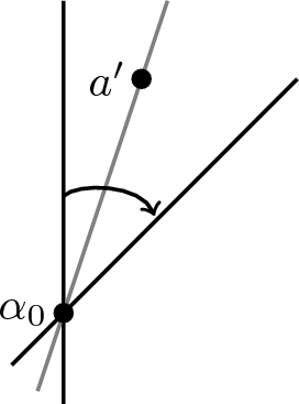
-
(b)
If instead we choose to set \(a'\) (\(=\alpha _1\)) as the new point about which the line rotates, we will let \(l_1\) represent the line through this point and note that
$$\begin{aligned} L_{l_1}= & {} L_{l_0}\\ R_{l_1}= & {} R_{l_0}\\ \overline{L}_{l_1}= & {} \overline{L}_{l_0}+p_{\alpha _1}-p_{\alpha _0}\\ \overline{R}_{l_1}= & {} \overline{R}_{l_0}-p_{\alpha _1}+p_{\alpha _0}. \end{aligned}$$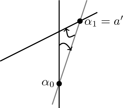
-
(a)
-
(c)
The point \(a'\) lies to the left of \(l_0\).
-
(a)
If we rotate past \(a'\), then the updated total weights become
$$\begin{aligned} L'_{l_0}= & {} L_{l_0}-p_{a'}\\ R'_{l_0}= & {} R_{l_0}+p_{a'}\\ \overline{L}'_{l_0}= & {} \overline{L}_{l_0}-p_{a'}\\ \overline{R}'_{l_0}= & {} \overline{R}_{l_0}+p_{a'}. \end{aligned}$$
-
(b)
However, if instead we choose to set \(a'\) (\(=\alpha _1\)) as the new point about which the line rotates, as above we let \(l_1\) represent this line and note that
$$\begin{aligned} L_{l_1}= & {} L_{l_0}+p_{\alpha _0}-p_{\alpha _1}\\ R_{l_1}= & {} R_{l_0}-p_{\alpha _0}+p_{\alpha _1}\\ \overline{L}_{l_1}= & {} \overline{L}_{l_0}\\ \overline{R}_{l_1}= & {} \overline{R}_{l_0}. \end{aligned}$$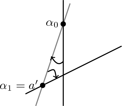
-
(a)


Given \(R_{l_0}\le I+p_{\alpha _0}\le I+\varepsilon\), and thus that \(I-\varepsilon \le L_{l_0}\le I\le R_{l_0}\le I+\varepsilon\), if \(a'\) lies to the right of \(l_0\), both of (1a) and (1b) will ensure the left-side and right-side weights remain within \(\varepsilon\) of I; that is, that the inequalities
hold upon rotation past \(a'\) or by replacing \(\alpha _0\) with \(\alpha _1\) (\(=a'\)) as the point of rotation.
If \(a'\) lies to the left of \(l_0\), we proceed based on whether
or
If the former, then (2b) implies, with \(\alpha _1=a'\), that \(I-\varepsilon \le L_{l_1}\) and \(R_{l_1}\le I+\varepsilon\), which means \(L_{l_1}\) and \(R_{l_1}\) remain within \(\varepsilon\) of I.
If the latter, we consider \(\overline{L}_{l_1}\) and \(\overline{R}_{l_1}\). Since \(\overline{L}_{l_0}=L_{l_0}+p_{\alpha _0}\) and \(\overline{R}_{l_0}= R_{l_0}-p_{\alpha _0}\), certainly
and thus (2b) allows us to conclude \(\overline{L}_{l_1}, \overline{R}_{l_1}\) remain within \(\varepsilon\) of I. Therefore, starting with \(I-\varepsilon \le L_{l_0}, R_{l_0}\le I+\varepsilon\) allows us to conclude, upon rotation through/about \(a'\), that the left- and right-hand side weights remain within \(\varepsilon\) of I.
Now assume either \(L_{l_i}, R_{l_i}\) or \(\overline{L}_{l_i}, \overline{R}_{l_i}\) are both within \(\varepsilon\) of I. Initially assume it is \(L_{l_i}, R_{l_i}\). If the next point encountered upon rotation about \(\alpha _i\) is \(a''\), and if \(a''\) lies to the right of \(l_i\), then proceed via (1b). If \(a''\) (\(=\alpha _{i+1}\)) lies to the left of \(l_i\) and \(R_{l_i}\le I\le L_{l_i}\), proceed via (2a). If, however, \(L_{l_i}\le I\le R_{l_i}\) and \(I-\varepsilon \le L_{l_i}+p_{\alpha _i}-p_{\alpha _{i+1}}\), then use (2b) to see that \(I-\varepsilon \le L_{l_{i+1}}\) and \(R_{l_{i+1}}\le I+\varepsilon\).
Otherwise consider \(\overline{L}_{l_i}\) and \(\overline{R}_{l_i}\). Since \(\overline{L}_{l_i}=L_{l_i}+p_{\alpha _i}\) and \(\overline{R}_{l_i}= R_{l_i}-p_{\alpha _i}\), certainly
and thus (2b) allows us to conclude \(I-\varepsilon \le \overline{L}_{l_{i+1}}, \overline{R}_{l_{i+1}}\le I+\varepsilon\).
As the other possible case, assume \(\overline{L}_{l_i}, \overline{R}_{l_i}\) are within \(\varepsilon\) of I. If the next point encountered, \(a''\), is to the left of \(l_i\), then (2b) implies \(\overline{L}_{l_{i+1}}, \overline{R}_{l_{i+1}}\) are within \(\varepsilon\) of I. Next assume \(a''\) (\(=\alpha _{i+1}\)) lies to the right of \(l_i\). If \(\overline{L}_{l_i}\le I\le \overline{R}_{l_i}\), proceed via (1a). If \(\overline{R}_{l_i}\le I\le \overline{L}_{l_i}\) and \(I-\varepsilon \le \overline{R}_{l_i}-p_{\alpha _{i+1}}+p_{\alpha _i}\), then proceed via (1b) to see that \(I-\varepsilon \le \overline{R}_{l_{i+1}}\) and \(\overline{L}_{l_{i+1}}\le I+\varepsilon\).
Otherwise consider \(L_{l_i}\) and \(R_{l_i}\). Since \(L_{l_i}=\overline{L}_{l_i}-p_{\alpha _i}\) and \(R_{l_i}=\overline{R}_{l_i}+p_{\alpha _i}\), certainly
and thus (1b) allows us to conclude \(L_{l_{i+1}}, R_{l_{i+1}}\) lie within \(\varepsilon\) of I.
In this way, we conclude that each point encountered will allow continued clockwise rotation past/about that point while preserving either \(L_{l_i}, R_{l_i}\) or \(\overline{L}_{l_i}, \overline{R}_{l_i}\) within \(\varepsilon\) of I.
Upon rotation through \(\pi\) radians, the line will now be oriented in the negative y direction. Call this line \(l_f\) and the point it contains \(\alpha _f\). We know either \(L_{l_f}, R_{l_f}\) or \(\overline{L}_{l_f}, \overline{R}_{l_f}\) are within \(\varepsilon\) of I. If \(\alpha _f=\alpha _0\), then \(l_f=l_0\); otherwise \(l_0\) and \(l_f\) are parallel. If parallel, the points lying strictly between \(l_0\) and \(l_f\) have a combined weight of at most \(2\varepsilon\). This means \(l_f\) can be translated horizontally so as also to contain \(\alpha _0\) without changing at any point along the way the fact that either \(L_{l_f}, R_{l_f}\) or \(\overline{L}_{l_f}, \overline{R}_{l_f}\) are within \(\varepsilon\) of I.
We now consider the points in B. Let \(\lambda _{l_0}\) represent the combined weights of the points in B strictly to the left of \(l_0\) and \(\rho _{l_0}\) the combined weight of the points in B strictly to the right of \(l_0\). Likewise for \(\lambda _{l_f}\) and \(\rho _{l_f}\) relative to the line \(l_f\). Then, since \(\lambda _{l_0}=\rho _{l_f}\) and \(\lambda _{l_f}=\rho _{l_0}\),
This means that at some point in the progression of lines from \(l_0\) to \(l_f\) there was an initial instance, say \(l_k\), where \(\lambda _{l_k} - \rho _{l_k}\) first had a sign opposite of that for \(\lambda _{l_0} - \rho _{l_0}\). Consequently, since \(|\lambda _{l_k} - \rho _{l_k}| = q_{b_k}\), it follows that
and therefore including the weight \(q_{b_k}\) with whichever of \(\lambda _{l_k}\) or \(\rho _{l_k}\) is smaller means the two sides’ combined weights are each within \(\overline{\epsilon }\) of \(\overline{I}\). \(\square\)
Multi-balanced redistricting
It is straightforward to apply this theorem to a redistricting-like problem in which the political unit will be divided into two districts, each balancing two separate quantities. Because the hypotheses of Theorem 1 do not require the points in A and B to be disjoint, we may take the points in A and B to have the same locations in the plane—such as those defined by the centroids of the geographic subunits that partition the area (e.g., census blocks, census block groups, or voting precincts). If necessary to satisfy the hypotheses of the theorem, apply a perturbation to one or more points. As points in A, these centroids may have weights corresponding to the population of the subunit. As points in B, the weights may be any other quantity for which district balance may be desirable, such as those noted in the introduction. As an illustration of the implementation, Fig. 3 shows census blocks and associated centroids for the city of Grand Forks, ND, along with the multi-balance split for 2020 populations and 2025 projected populations.

Census blocks, census block centroids, and multi-balanced division for the city of Grand Forks, ND, based on actual 2020 and projected 2025 populations
Of course, there are limitations to the applicability of this approach. One such instance occurs when \(\max \{p_{a_i}\}\) or \(\max \{q_{b_i}\}\) exceeds the allowed threshold for population deviations. This extreme situation is unlikely to occur in larger geographic regions with a significant number of subdivisions, but may be present with smaller municipal redistricting instances where a large imbalance in population counts across subdivisions occurs.
A second obvious limitation concerns instances where the desired number of districts is not a power of 2. We deal with such a situation momentarily, but start by noting that when a number of districts equal to an arbitrary power of 2 is desired, one simply carries out further subdivisions. Because in this case, the deviations from the ideal balance may compound with each step, the following corollary provides an upper bound on the deviation that is independent of the number of subdivisions used.
Corollary 1
Let \(\mathcal {C}\) be a collection of geographic units which collectively partition the region \(\mathcal {R}\). Let \(\{p_i\}\) and \(\{q_i\}\) represent the quantities to be balanced. For any integer \(N\ge 1\), it is possible to divide \(\mathcal {C}\) into \(2^N\) contiguous subregions so that each subregion deviates from the ideal values of
by no more than \(2\max \{p_i\}\) and \(2\max \{q_i\}\), respectively.
Proof
Without a loss of generality, we focus on the weights \(\{p_i\}\). For integers \(n, j\ge 1\), let \(P_{n,j}\) represent the total of these weights for the j-th district after the n-th division. Let \(I_{n,j}\) represent the best-possible value for the division of \(P_{n,j}\), i.e., \(I_{n,j}= P_{n,j}/2\). With \(I_{0,1}=(1/2)\sum {p_i}\) being the initial ideal weight balance, we know from the theorem above that
where \(\varepsilon = \max \{p_i\}\). This implies
and so from
and
we obtain
from which it immediately follows that \(P_{2,j}\) is within \(2\varepsilon\) of its ideal value.
In a similar fashion, for any \(n\ge 1\), if we know
then
Since for \(l\in \{2j-1, 2j\}\), we have \(I_{n,j}-\varepsilon \le P_{n+1,l}\le I_{n,j}+\varepsilon\), we conclude
implying \(P_{n+1,l}\) is within \(2\varepsilon\) of its ideal. \(\square\)
To realize a division of a region into a non-power-of-2 number of districts, say M, for which the features described by the weights \(\{p_i\}\) and \(\{q_i\}\) are simultaneously balanced, one chooses a sufficiently large n, divides the region into \(2^n\) subregions, and then consolidates these \(2^n\) subregions into M districts. Of course, this will introduce further instances in which imbalances in the \(2^n\) subregions may compound.
For instance, unless M is a power of 2, some districts will consist of \(\lceil 2^n/M\rceil\) subregions. If each of these happens to exceed its ideal population by the maximum possible amount, the resulting subregion’s population will be
where P is the total population of the state. The ideal subregion population is P/M, and thus the maximum fractional deviation from ideal is the following function of n and M:
Taking the state of North Dakota (ND) as an example, in which case the values of \(P=756,508\) and \(\varepsilon = 17,279\) represent estimates of voting precinct population based on data published by [21], we obtain the results in Table 1, which show the maximum fractional deviations from ideal based on the above formula.
The utility of these estimates clearly breaks down for some combinations of n and M. And even in the best case illustrated in the table, the balance is not particularly good. Of course, for these upper bounds to be realized requires both that
-
(1)
The process of creating districts proceeds first by dividing the region into \(2^n\) subregions which are then reconsolidated to form M districts; and
-
(2)
One of the reconsolidated districts is formed entirely from subregions all of which exceed their ideal balance by the maximum theoretical amount.
Given the conditions necessary to achieve this worst-case scenario, it is unlikely that many practical realizations of multi-balanced districts would be so poorly out-of-balance in both properties. And in fact, in the section below we present empirical evidence from actual state redistrictings that demonstrates the practicality of obtaining reasonable multi-balanced redistrictings.
A stochastic optimization approach to multi-balanced redistricting
We conclude this paper by describing an empirical example of multi-balanced redistricting using data from the 2020 redistricting cycle. We use the 10 Congressional districts of Washington state as a case study, balancing the 2020 Census population one at a time against additional baselines reflecting the potential use cases discussed in the introduction. Specifically, we use 2030 block level projections as a comparison of future-proofing districts against within-cycle malapportionment, the 2020 census voting age population, the 2015–2019 Population data from the ACS, and the official block-level population totals adjusted for individuals in state custody as described in the Rules Code of Washington (RCW) 44.05.140 [27]. In each experiment, we attempt to balance districts according to both the 2020 Census populations and a single one of the other population types. The underlying dual graph was formed from 2020 Census Block Groups and the data was aggregated from the Census API, NHGIS, and the Redistricting Data Hub.
To generate the plans, we use a variant of the ReCombination algorithm described in [13] to perform an iterative optimization approach, alternating between shrinking the deviations of the two relevant population columns. After taking 100 ReCombination proposals starting from a randomly constructed plan, constrained only by the Census population, we implement a local-search procedure using 100,000 proposals of the Flip-Walk to find approximate local optima of the sum of the dual population imbalances. This approach is motivated by the process introduced in [12], which used a similar method to generate plans with a large number of competitive districts. A combination of ReCombination and Flip proposal methods for optimization of districting plans was also employed in [6] to study several redistricting criteria. This is not intended to be an exhaustive or optimal example but rather presents a feasible case study demonstrating the ease of implementing these methods and surpassing the theoretical worst-case bounds. In particular, taking additional steps to prove local optimality, exploring the global space with multiple runs, and refining the choice of target metric are interesting questions for future work. Code and data for replicating these experiments can be downloaded from [14].
The results of this experiment are shown in Table 2, demonstrating that it is possible to create plans that outperform the worst-case bounds described in the previous section for each of the empirically relevant cases described in the introduction. At the end of the ReCombination run, most of the secondary columns had deviations over 11% of ideal but the local optimization procedure succeeded at decreasing those significantly. An example of this decrease in deviation, measured in the percent of ideal deviation between the largest and smallest districts over the course of the optimization run for the VAP data is shown in Fig. 4. Results for the other sets of population data demonstrated similar behavior.

Decrease in VAP deviation from ideal over the local optimization steps. The horizontal axis shows the number of flip steps performed, while the vertical axis shows the difference between the largest and smallest districts as a percentage of the ideal population
The success of these experiments using straightforward and computationally limited methods suggests that multi-balance could be taken into account as a practical concern by line drawers in future redistricting cycles looking to prevent or minimize the impact of within-cycle malapportionment. In particular, analysis with projected populations could help address concerns about voter dilution in urban areas over the course of the decade. It could also help reconcile state-level demands to account for incarcerated populations or other constraints while still generating plans that are balanced according to the Census totals.
Conclusions and future work
In an extreme (but unrealizable) case where it would be possible to partition a region down to the single-voter level, [24] describes how results found in [8, 18, 23] would allow balanced partitions into any (non-power-of-2) number of convex subsets. The present paper provides a partial generalization of these results by proving multi-balancing is always possible to within reasonable tolerances. These results apply directly only when the number of districts is equal to a power of 2, however, computational results illustrate that excellent multi-balancing is feasible for numbers of districts not equal to a power of 2. This establishes the practicality of multi-balanced redistricting.
Of course, in light of the discussion in [24], a natural extension to the results of this paper would be to prove that two sets of weighted points may be directly subdivided into an arbitrary number of convex subregions, each of which is balanced for both sets of weights. Both [8] and [23] provide approaches that may be fruitful for obtaining such a generalization. Another generalization more closely tied to the redistricting context might exploit the correlation at the level of nodes between the relevant weight values.
And what of the possibility of simultaneously balancing more than two features? A simple example, such as that below, illustrates there are no guarantees (Fig. 5). In this example, any attempt to balance, say, the weight-1 values will necessarily involve a line splitting the four points in the upper left into two nonempty subsets. If one is further interested in simultaneously balancing the weight-2 values, the line doing so necessarily also divides the points in the upper right cluster. But then all points in the lower center are entirely on one side of this line, making the weight-3 values unbalanced. Despite this example, to what extent might triple-balancing be a realistic goal for typical real-world situations, where correlations are likely to exist between the weights to be balanced? We leave for future work an application to a realistic example for determination of the possibilities and limitations.

Example set of points with three columns that does not admit a nearly balanced partition
Data availability
The raw data used in this paper is publicly available from [20, 21] and https://redistrictingdatahub.org. Replication code for the empirical experiments is available at [14].
Notes
This is sometimes referred to as “eligible-voter” redistricting where the plans are balanced according to citizen, voting-age population, or CVAP.
References
AAJC, MALDEF, and National Conference on Citizenship (Organizers): Statement on Appropriate Data for Redistricting, https://www.advancingjustice-aajc.org/sites/default/files/2021-04/Statement%20on%20Appropriate%20Data%20for%20Redistricting%20FINAL%204.27.2021.pdf, (2021).
Alexeev, Boris, & Mixon, Dustin G. (2018). Partisan gerrymandering with geographically compact districts. Journal of Applied Probability, 55(4), 1046–1059. https://doi.org/10.1017/jpr.2018.70
Badger, E.: People Who Can’t Vote Still Count Politically in America. What if That Changes?, New York Times Upshot, (2019).
Bar-Natan, A., Najt, L., & Schutzman, Z. (2020). The gerrymandering jumble: map projections permute districts’ compactness scores. Cartography and Geographic Information Science, 47(4), 321–335.
Barnes, R., & Solomon, J. (2021). Gerrymandering and Compactness: Implementation Flexibility and Abuse. Political Analysis, 29(4), 448–466.
Becker, A., & Gold, D. (2022). The gameability of redistricting criteria. Journal of Computational Social Science, 5, 1735–1777.
Bernstein, M., & Duchin, M. (2017). A formula goes to court: Partisan gerrymandering and the efficiency gap. Notices of the American Mathematical Society, 64(9), 1020–1024.
Bespamyatnikh, S., Kirkpatrick, D., & Snoeyink, J. (2000). Generalizing ham sandwich cuts to equitable subdivisions. Discrete and Computational Geometry, 24(4), 605–622.
Boland, J., Rudensky, Y., & Li, M. (2021). Why States Should Wait for Census Data to Draw Voting Districts , Brennan Center for Justice Report, https://www.brennancenter.org/media/7532/download,
Chen, Jowei, & Stephanopoulos, Nicholas. (2021). Democracy’s Denominator. California Law Review, 109, 1019–1065.
DeFord, D., Dhamankar, N., Duchin, M., Gupta, V., McPike, M., Schoenbach, G., & Sim, K. (2021). Implementing partisan symmetry: Problems and paradoxes, Political Analysis, 1-20.
DeFord, D., Duchin, D., & Solomon, J. (2020). A computational approach to measuring vote elasticity and competitiveness. Statistics and Public Policy, 7(1), 69–86.
DeFord, D., Duchin, D., & Solomon, J. (2021). ReCombination: A family of Markov chains for redistricting, Harvard Data Science Review, 3(1),
Deford, D., Kimsey, E., & Zerr, R. (2022). Replication Data and Code for WA experiments in “Multi-Balanced Redistricting”, https://github.com/drdeford/MBR_WA.
Duchin, M., & Tenner, B. E. (2018). Discrete geometry for electoral geography, arXiv:1808.05860.
Edelman, P. H. (2016). Evenwel, Voting Power, and Dual Districting. Journal of Legal Studies, 45(1), 203–221.
Hirsch, S. (2003). The United States House of Unrepresentatives: What Went Wrong in the Latest Round of Congressional Redistricting. Election Law Journal, 2(2), 179–216.
Kaneko, A., & Kano, M. (1999). Balanced partitions of two sets of points in the plane. Computational Geometry: Theory and Applications, 13, 253–261.
Katz, J., King, G., & Rosenblatt, E. (2020). Theoretical Foundations and Empirical Evaluations of Partisan Fairness in District-Based Democracies. American Political Science Review, 114(1), 164–178.
Manson, S., Schroeder, J., Van Riper, D., Kugler, T., & Ruggles, S. (2021). IPUMS National Historical Geographic Information System: Version 16.0 [dataset], Minneapolis, MN: IPUMS. https://doi.org/10.18128/D050.V16.0
NDSU Center for Social Research: ND Compass: State Legislative District Profiles, available at https://www.ndcompass.org/legislative-district-profiles/, accessed on 23 May 2021.
Rudensky, Y., Li, M., & Lìmon, G. (2021). The Impact of Census Timeline Changes on the Next Round of Redistricting, Brennan Center for Justice Report, https://www.brennancenter.org/media/7532/download
Sakai, T. (2002). Balanced convex partitions of measures in \(\mathbb{R} ^n\). Graphs Combin., 18(1), 169–192.
Soberón, P. (2017). Gerrymandering, sandwiches, and topology. Notices of the American Mathematical Society, 64(9), 1010–1013.
Stephanopoulos, Nicholas, & McGhee, Eric. (2015). Partisan Gerrymandering and the Efficiency Gap. University of Chicago Law Review, 82, 831–900.
Ueckerdt, T. (2021). Lecture Notes: Combinatorics in the Plane, available at https://www.math.kit.edu/iag6/lehre/combplane2013s/media/lecture_notes.pdf, accessed on 21 May
Washington State Legislature: Rules Code of Washington: 44.05.140 Residence of certain individuals-Last known place of residence., https://app.leg.wa.gov/Rcw/default.aspx?cite=44.05.140, accessed May 11, 2023.
Acknowledgements
E. K. was supported by the Ellen Hauge Abelson Scholarship for undergraduate research from the Washington State University College of Arts and Sciences.
Author information
Authors and Affiliations
Corresponding author
Ethics declarations
Conflict of interest
D. D. has previously served as an expert in redistricting cases. E. K. and R. Z. have no conflicts to report.
Additional information
Publisher's Note
Springer Nature remains neutral with regard to jurisdictional claims in published maps and institutional affiliations.
D. DeFord: https://scholar.google.com/citations?user=nE14CxwAAAAJ&hl=en.
Rights and permissions
Springer Nature or its licensor (e.g. a society or other partner) holds exclusive rights to this article under a publishing agreement with the author(s) or other rightsholder(s); author self-archiving of the accepted manuscript version of this article is solely governed by the terms of such publishing agreement and applicable law.
About this article

Cite this article
DeFord, D., Kimsey, E. & Zerr, R. Multi-balanced redistricting. J Comput Soc Sc 6, 923–941 (2023). https://doi.org/10.1007/s42001-023-00217-8
Received:
Accepted:
Published:
Issue Date:
DOI: https://doi.org/10.1007/s42001-023-00217-8