
Abstract
Early-stage breast cancer detection remains a critical challenge in healthcare, demanding innovative approaches that leverage the power of deep learning and transfer learning techniques. The problem to be investigated involves designing a model capable of extracting meaningful features from mammographic images, maximizing transferability across datasets, and optimizing the trade-off between model complexity and computational efficiency. Existing methods often face limitations in achieving high accuracy, robustness, and efficiency. This research aims to address these challenges by proposing a novel transfer learning approach that combines the strengths of VGG11 and EfficientNet architectures for early-stage breast cancer detection. In the case of technological development, there is never a shortage of opportunities in the field of medical imaging. Cancer patients who have an earlier diagnosis of their disease have a lower probability of passing away from their illness. This research proposed an novel early neural network based on transfer learning names as ‘EARLYNET’ to automate breast cancer prediction. In this research, the new hybrid deep learning model was devised and built for distinguishing benign breast tumors from malignant ones. The trials were carried out on the Breast Histopathology Image dataset, and the model was evaluated using a Mobile net founded on the transfer learning method. In terms of accuracy, this model delivers 91.53% accuracy. Explored how the proposed transfer learning framework can enhance the accuracy and reliability of early-stage breast cancer detection, contributing to advancements in medical image analysis and positively impacting patient outcomes.
1 Introduction
Cancer ranks among the top five leading causes of death in the world. It has been reported that around one in every 37 people who have breast cancer will pass away as a direct result of the disease (Dora et al. 2017). An automated and efficient cancer predictive model can, as a point of fact, help with timely diagnosis and, as a corollary, reduce the death rate associated with cancer. Breast cancer claimed the lives of at least 684,996 women worldwide in 2025, according to official estimates (New York State Department of Environmental Conservation 2009). With an age-adjusted incidence rate as high as almost twenty-five women per one lakh and a fatality rate of approximately twelve to thirteen per 100,000 women, breast cancer has been listed as the most prominent form of cancer among Indian females. The incidence and mortality rates of cancer were compared using data reports from a variety of the most recent national cancer registries (Malvia et al. 2017).
Breast Cancer is a condition wherein breast cells proliferate uncontrolled. A carcinoma kind is categorized by the malignant cells. Breast cancer can begin in any area of the breast. The breast is divided into three sections: connective tissue, lobes, and ducts. The majority of this type of cancer begins in the ducts or lobules. Invasive ductal carcinoid tumors are the utmost prevalent morphological subset of all Breast cancers constituting about 80 percent of them (DeSantis et al. 2011). Specialists typically diagnose this via visual examination of tissue slides or a digital mammography. Mammography is a type of breast imaging used by radiologists to detect early signs of adenocarcinoma in the breast region affecting women. Analysis of illness severity is largely restricted to locations having invasive carcinoma (Elston and Ellis 1991). Therefore, the initial phase in the histopathological evaluation of retrieved breast tissue is to discriminate amongst tissue regions pertaining towards intrusive lump as well as non-intrusive tissues (Arya and Saha 2020). Segregating invasive ductal carcinoma allows for additional study of tumor differentiation by Bloom-Richardson-Nottingham grading systems (Genestie et al. 1998). This carcinoma detection procedure is a lengthy and demanding one partly because it needs a pathologist screening on broad expanses of benign areas to get results leading towards the locations of the malignance. Detailed identification of ductal adenocarcinoma is important to reach the successive calculation of classifying tumour hostility and foreseeing patient outcome (Cruz-Roa et al. 2014).
The classic Computer-aided Diagnosis for breast cancer has three steps. It starts with discovering the Contour of Interest in the precompiled mammogram, which is the region where the tumour is. Secondly, expert knowledge is used to extract features of the tumour, such as its structure, appearance, and density, so that feature vectors can be extracted manually. Lastly, these feature vectors can be used to distinguish and categorize between benign and cancerous tumours (Kumar et al. 2022). The effectiveness of the customized feature set directly influences the predictive performance of the diagnosis, and as a result, an expert physician plays a very important role here to process the manually extracted features (Chen and Lin 2014; Ganesan et al. 2012). The generally employed traits, which are derived from the experience of the physicians, are referred to as the subjective features. In recent times, numerous deep learning techniques are effectively implemented to retrieve stratified attributes from visual information alone without conventional procedure (Seedat and Aharonson 2021). These retrieved characteristics are also referred to as objective attributes (Dar et al. 2022).
Significant contribution made in this work are as follows:
-
Improved the effectiveness in learning low-level features, while EfficientNet excels at learning more complex and higher-level features. By combining these two architectures, the transfer learning model can extract both low-level and high-level features, resulting in more informative representations.
-
Developed a Novel Transfer learning leveraging pre-trained models (VGG11 and EfficientNet) that have been trained on large-scale datasets.
-
Enhanced the state-of-art performance by combining the VGG11 and EfficientNet architectures.
This paper proposes a superlative deep learning method to classify cancer and non-cancer images and a comparative study on experimental results from this novel model and existing techniques. In section II, a review of related methods are discussed. The methodology for this model is featured in the section III. Section IV is decorated with the investigational outcomes, and farther discourse about the work and comparison study with other related techniques, and section V takes the paper to the conclusion.
2 Literature review
Many studies have been done to look at how well mammograms can find tumours. Numerous studies have utilized conventional texture scrutiny (Hamouda et al. 2017), extreme learning machine (Xie et al. 2016), then random forest classifier (Dhungel et al. 2015) to categorize the images from mammography from the designated dataset into regular, benign, or malignant tumours (Pereira et al. 2014). Various studies have developed the use of IRMA dataset in order to categorize mammograms utilizing histogram oriented gradient (HOG) (Jadoon et al. 2017; Shastri et al. 2018).
Since years, various convolutional networks presented successful results on bigger sized image datasets (Krizhevsky et al. 2012). ILSVRC architecture by Russakovsky et al. is such a technique which leads to numerous working models for image classification which are of big-scale (Deng et al. 2014). With time, there were more attempts for improvement of these architectures to reach better accuracies (Malebary and Hashmi 2021) Due to advancement of the computer vision arena, newer models emerged to work out on different kinds of datasets to get outcomes with more precision using modified features in different convolutional layers (Sermanet et al. 2014; Zeiler and Fergus 2014). Developing neural networks with layering of higher depths, is more challenging because network depth is an important feature (He et al. 2015), leading to batch normalization (Ioffe and Szegedy 2015), to multi-scale processing (Szegedy et al. 2015). So arises newer problems. As the size of the network grows, accuracy gets stale to staler as all systems are similar, so they cannot be augmented by applying the same methods. Thus comes the deep residual learning model as a solution to this issue (Ren et al. 2016). To get a better performance out of a model, scaling up the feature helps out. These features can be the breadth and depth of the network used in the model, the resolution of images used as dataset etc. (Tan and Le 2019). Ciresan et al. (2013) utilized intense max-pooling CNN to find mitosis and grade breast cancer at the primary stage (Tzikopoulos et al. 2011).
Later, Pandian, Pasumpon (2019) proposed a Capsule Neural Network where MRI dataset is utilized, to get 90% accuracy. In Zhan Xiang et al. (2019), a convolutional neural network is presented where BreaKHis Database is used to get 97.2% accuracy. Peng Shi et al. (2019) presented a CNN technique which is referred as BI-RADS density classification to get 83.9% accuracy. More recently, Xinfeng Zhang et al. (2020) brought d-AE Neural Network, which is a Linear Discriminant Analysis, to get 98.27% precision. In Prakash et al. (2020), a Deep Neural Network design was presented where UCI dataset was used leading up to 98% accuracy (Prakash and Visakha 2020). This leads to a significant increase in accuracies in a variety of applications. This field combines aspects of machine learning and Neural Network (Abunasser et al. 2022). In this approach, numerous nonlinear computational tiers are used to extract characteristics directly out from data. The great degree of precision that DL techniques are capable of achieving in visual recognition can be attained in unison with analysis by specialists and doctors (Abunasser et al. 2023). The goals of this research are to achieve more accurate forecasts of the diagnosis of tumours and to achieve a more in-depth classification of observations. The drawbacks of the existing techniques are ensuring generalizability in the models by considering the variations in the breast tissues and its complex structure.
2.1 Problem statement and objective
Breast cancer is a significant global health issue, and early detection plays a crucial role in improving patient outcomes and survival rates. Traditional breast cancer detection methods, such as mammography, have limitations in terms of accuracy and sensitivity. Mammogram images in the dataset may exhibit variations in quality, such as differences in resolution, orientation, and compression artifacts, which can affect the model's ability to extract relevant features Therefore, there is a need to develop more accurate and efficient detection methods to aid in early diagnosis and treatment planning.
The objective of this research is to develop a deep learning-based system for breast cancer detection using medical images, particularly mammograms and histopathological images. The system will be designed to accurately classify breast cancer cases into malignant and benign categories based on the visual patterns and features present in the images. The main challenges in this problem include handling large and complex medical images, dealing with class imbalance in the dataset, and achieving high accuracy and robustness in the detection process.
3 Methodology
The methods used in the study might include multiple data visualization, data production, the building of a deep learning structure, and fine-tuning of the model for improved accuracy. The primary focus of this research is on the field of identifying breast cancer. According to the findings of research, the aforementioned actions are the ones that should be taken in order to have the best chance of accurately detecting breast cancer in the data. Figure 1 depicts the block diagram for this proposed early breast cancer detection system.

Block diagram of the methodology
-
a)
Dataset.
Invasive ductal carcinoma, or IDC, is the most frequent variant of breast carcinoma overall. The sections of a whole mount specimen that contain the IDC are often the ones that the pathologist concentrates on when attempting to allocate a severity score to the sample. As a consequence of this, one of the pre-processing stages that is typically included in automated severity scoring is to designate the specific sections of IDC that are contained inside a whole mount slide. The primary dataset was comprised of 162 full mount slide pictures of Breast Carcinoma specimens that were scanned at a magnification of 40 times. This resulted in the creation of 277,524 patches with a size of 50 by 50. Among these patches 198,738 ones were negative IDC, and 78,786 patches were positive IDC patches.
-
b)
Dataset visualization.
The data plays the major role in developing the architecture for the diagnosis of breast cancer so the data visualization stages an important part in it. The data visualization can define as the graphic depiction of data and information is the focus of the multidisciplinary discipline of data and information visualization. When there is a great deal of data or information to convey, such as in the case of a time series, this kind of communication is very effective. In addition to this, it involves the investigation of ways in which pictorial illustrations of intangible facts might improve human reasoning. The intangible facts consist of both numerical and non-numerical information, like typescript and topographical statistics, among other types of information. It is connected to infographics as well as the visualization of scientific data. Information visualization is when the spatial depiction (as an example, the folio layout of a graphical design) is selected, but scientific visualization is when the spatial representation is supplied. This distinction is one way to tell the two types of visualizations apart.
Figure 2 provides an explanation of many perspectives on the breast cancer data, which may be used as a foundation for defining the feature extraction procedure. The data paints a clear picture regarding the distinct characteristics of a variety of different subjects in relation to breast cancer.
-
c)
Feature extraction utilizing image sampling.

Multiple data visualization of dataset
Through the use of grid sampling, each WSI is cut up into image patches that do not overlap and measure 100 by 100 pixels. Discarded are patches that are predominantly composed of fatty tissue or those that have a slide backdrop. The sections of the genome that contain IDC are physically glossedby a diagnostician for training. Then, this manual annotation is employed to create a binary annotation mask. In order for an image area to be considered a positive sample, the annotation mask necessarily should cover at least 80% of the patch’s area. In the event that this is not the situation, the patch will be evaluated as a negative sample.
Figure 3 provides a description of the images while they are undergoing the sampling process, which is a procedure that is extremely committed to the process of feature extraction. Figure 3 provides a description of the pictures that are produced after image sampling has been completed and before the feature extraction data of the raw image are created.

Images used in the sampling processes
In Fig. 4, the tissue on the left does not have any target information associated with it. The identical tissue is depicted on the image on the right, and the presence of cancer is indicated by the intense red stain.
-
d)
Data fragmentation.

Sampled image
The dataset is split into 3 parts. Almost 69.89 percent of the 277,524 thermal images were utilized as training set of data. 15 percent of the main set of data were used for validating the model and to test the model output, there were another 15 percent of this dataset. Figure 5 depicts the comparison of 3 different datasets. In Fig. 6 the sampled training images are presented.

Illustration of data comparison of cancer patches to healthy tissue patches in 3 data subsets. The test data has more cancer patches compared to healthy tissue patches than train or dev

Sampled training images
-
e)
Deep learning architecture.
Deep learning is a subclass of a broader brood of machine learning algorithms those are focused on neural nets and pattern recognition. It is also referred to as deep structured learning. There are three distinct approaches to learning, which are the supervised, semi-supervised, and uncontrolled learning environments. Computer vision, NLP, Bioinformatics, climate science, speech-recognition, language processing, drug design, material inspection, medical photo analysis, and board game coding are just some of the areas that have benefited from the application of deep-learning architectures. These applications have generated results that are on par with, and in some cases even better than, those generated by conventional machine learning approaches.
The open-source deep learning framework known as pytorch is used to construct the Deep Learning model that is used in this investigation.
3.1 Residual learning
The model devoted to the activation function of RELU, which displays superior performance in accordance with the findings of this study. In neural network topologies, network depth plays a significant role, yet deeper networks are harder to teach. The residual learning model makes it easier to train these networks and allows them to be much deeper, resulting in enhanced efficiency for image dataset (He et al. 2016).
Instead of working under the assumption that each stack of layers will directly match a specified underlying mapping. The residual learning model allows the layers to fit a vestigial mapping. The initial mapping is rewritten as F(x) + x in this iteration. The hypothesis here is that refining the mapping of the residuals will be less difficult than refining the mapping of the original, unreferenced data. If such an identity map was the best possible solution, the most extreme case might be that it would be simpler to reduce the residual to zero than it would be to suit an identity mapping using a series of nonlinear layers. Rather than developing the desirable result from beginning, succeeding blocks in this model network are accountable in fine-tuning the outcome of a prior block. This frees them from producing the output from scratch. Figure 7 shows a fundamental block for RELU model.

The rudimentary structural block of residual network model
3.2 The mobilenet model-based transfer learning
MobileNets are a type of light-weight deep CNN layers, which is much smaller and performs much faster than most other popular models. MobileNet makes use of depth-wise separable convolutions in its processing. MobileNet makes use of depth-wise discrete convolutions in its processing. In comparison with a network with conventional convolutions of the same depth in the nets, it dramatically decreases the number of parameters. As a result, compact deep neural networks are created. The Fig. 8 (Tan and Le 2019) is shown below.

Block diagram of mobilenet a depthwise convolution for the spatial convolution layer, b pointwise convolution to change the dimension
3.3 The efficientnet model-based transfer learning
Transfer learning is a way of increasing knowledge in a new task via transmitting information out of an obtained related task. This allows the learner to improve their performance in the new activity. Transfer learning, in particular, reduces time and enhances performance. For example, a model that can recognize the helicopters can now recognize the air planes using a pre-trained model. EfficientNet is based on the premise that offering an effective compound scaling approach for expanding model size can assist the model achieve maximum accuracy. It begins with the multifactorial scaling method. The first stage in the compounded scaling approach is to do a lattice survey to determine the interactions between various scaling parameters of the base network. This calculates the proper scaling coefficient in every single one of the dimensions. Then those factors are applied to ramp up the foundation system to the appropriate target pixel pitch. The efficacy of system scaling also relies largely on the foundation system. The concept of Efficientnet utilizes mobile inverted bottleneck convolution with scaled up baseline network to generate a group of models. The Fig. 9 (Tan and Le 2019) is shown below.

(Source: Mingxing et al. (Tan and Le 2019)
Visualization of various scaling
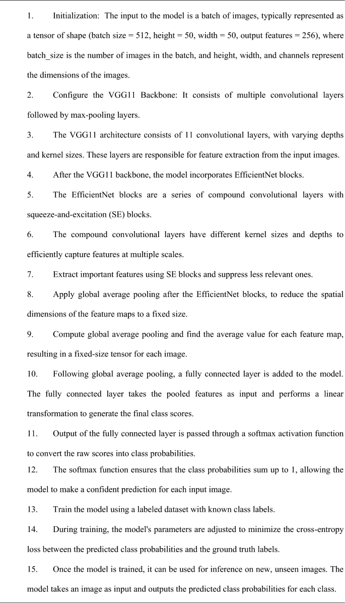
3.4 The proposed novel deep learning method based on transfer learning utilizing VGG11 Efficientnet for breast cancer diagnosis
Here, in our case of the novel deep learning model using a deep learning classifier model based on transfer learning is built with thirty-two batches, each of which has its own batch normalization and dropout ratio of 0.75. In this way, this constructed VGG11 (Visual Geometry Group) Efficientnet- based Hybrid Deep Neural model is employed to train on the data obtained from the fragmented datasets after splitting the pre-processed image dataset into three parts. In VGG-11, it has 11 weighted layers, which describe the intensity of linkages among entities in neighboring network layers. Weights around zero mean that modifying this input will have little effect on the output. There are three nodes on VGG-11 that are all connected to one another. The graphical representation depiction of the same can be found in the given Fig. 10. The two upper fully-connected segments have a total of 4096 channels. Because each channel corresponds to a single class, the 3rd completely-connected level comprises a total of one thousand channels. VGG works with the depth of convolutional neural networks. It is a model that has already been trained on a dataset, and it has weights that are meant to represent the characteristics of the dataset on which it was trained. The Efficientnet based on transfer learning is the foundation for the VGG-11 model employed here in this study. When one uses a model that has already been trained, they save time. Learning a large number of features has already used a significant amount of time and processing capacity, and it is probable that the model will gain an advantage as a result of this.

The flow diagram of VGG11 network model
Stochastic gradient descent was employed here as the fine-tuning method to generalize the outcome of the model when applied on a new dataset with which the model was not familiar. Stochastic gradient descent uses only a random subset for each iteration instead of using the entire dataset. The learning rate was set at 0.01 for the experiment. After that, an assessment was done on various neural network models following a comparison study to know the comparative accuracy rate for this technique.
-
f)
The algorithm.
The algorithm for our proposed model for the prediction of early diagnosis of breast cancer is presented below:
Algorithm: EarlyNeuralNet: A Novel Transfer Learning Algorithm VGG11-EfficientNet Networks.

4 Results and discussion
-
a)
Assessment of the DL Process
The outcome of this research is designing a model for categorizing cancer and non-cancer images to spot breast adenocarcinoma in the beginning phase. We utilized PyTorch for training the model. Our hybrid model based on transfer learning utilizing VGG11 Efficientnet reached a categorization accuracy of adenocarcinoma and non-cancer cells to 83.23% during training at the last epoch. The error in the model during training came out to be 38.91%. In this case study, we found the proposed hybrid model’s testing loss to be 32.41%. During testing of the VGG11 Efficientnet-based transfer learning model when employed on the test data patch, the accuracy percentage reached 87.91%. The details of accuracy and loss values for our proposed hybrid method are presented in Table 1.
In this work, we employed various instances of transfer learning on the image dataset patches. The basic concept of transfer learning is to transmit what a model has learnt from one task with ample labelled training data to one with little data. We employ patterns already established while completing similar work to speed up the learning process. Given the massive amount of CPU power required, transfer learning is typically employed in image-based analysis tasks. Here, we utilized three models for training, testing and validating the models and finding the model accuracy in detecting adenocarcinoma from image data. These transfer learning test cases are, respectively, Mobilenet model-based, Efficientnet model-based, and a proposed hybrid model-based which is formed utilizing VGG11 Efficientnet.
We utilized sampled image (shown in Fig. 4) after pre-processing the tissue-image patches as required to automate the diagnosis of adenocarcinoma. The tissue on the left side of Fig. 4 does not contain any relevant data connected to it. On contrary, the image on the right side depicts the same tissue as the left, the prevalence of cancer is shown by the deep red stain.
The residual networks used here are far more profound than their ‘simple’ equivalents but require the same number of weights. Here, the layers are taken directly from the shallower model that was.
previously learned, and the addition of the new tiers is identity mapping. Due to the fact that this created solution exists, it can be deduced that a model of higher depth should not produce a higher level of training error than its counterpart, which is shallower. For the RELU model, fine-tuning is done using the zero_grad optimizer. Zero_grad optimizer fixes the grads to None instead of setting it as zero. Fine-tuning is done to improvise the outcome to be better.
-
b)
The performance of the model
The performance of the model is computed using different factors, which are true positive (TP), true negative (TN), false positive (FP), and false negative (FN). The following equations (Eqs. 1–4) are utilized for the performance parameters calculation of this study.
$$epsilon = 1e - 7$$(1)$$precision = \frac{tp}{{\left( {tp + fp + epsilon} \right)}}$$(2)$$recall = \frac{tp}{{\left( {tp + fn + epsilon} \right)}}$$(3)$$f1score = \frac{2 \times precision \times recall}{{(precision + recall + epsilon)}}$$(4)
The accuracy of this model’s output is 77.15%. EfficientNet is a collection of convolutional neural network models which increases accuracy as well as model efficiency by dropping the amount of factors used for assessment with other related models. Here, In the case of the Efficientnet model- based transfer learning, stochastic gradient decent (SGD) was used as optimizer for fine-tuning. In the case of MobileNets, these models have been customized to meet the resource limits of a variety of use cases. As a result, they have a fast response time and consume a low amount of power. Segmentation, categorization, identification, embeddings, can all be constructed on top of them.
The proposed hybrid deep learning model utilizing VGG11 and Efficientnet transfer learning uses stochastic gradient decent (SGD) as the optimizer resulting the outcome accuracy for this proposed model as 91.53%. The fine-tuning was not applied on the proposed model directly. The optimizer was used after various trial and error processes to get a better accuracy percentage. If, farther studies are done on pre-processing, model training or optimizer tuning, this model can be improvised to get a higher accuracy in the future.
-
c)
Performance Comparison in contrast to other Models: This is shown in Table 2.
In Fig. 11, comparison plots are generated due to training losses, validating losses and testing losses for different deep learning models.

Comparison of losses among training (red), validating (blue) and testing (green) datasets for different deep learning models
In Fig. 12, resent the comparison plot of the losses incurred during training (shown in blue), validating (shown in orange), and testing (shown in green) using the novel deep learning technique that makes use of VGG11 Efficientnet. The plot shows that training and validation losses are gradually declining and steadying at specific points, making this approach well-fitted.

The comparison of losses among training (blue), validating (orange) and testing (green) data patches for the proposed novel deep learning method based on transfer learning utilizing VGG11 Efficientnet
Table 3, shows the comparison of state of art models balanced accuracy with proposed model, from the obtained result it shows that the proposed EarlyNet gives the better accuracy with 91.53% than the state-of-art models such as 2D CNN, AlexNet with BN and Inception Net. An observation of this study is that the miscategorized cell sections are probably because of the consequence of insufficient tags provided by annotators than errors in the procedure we have projected. The most notable quality of our method is that it is capable of being reproduced with a variety of unseen data. This reproducibility is almost equivalent to the interpretive bitwise mechanical labelling that trained pathologists would produce with minute details.
5 Conclusion
In this research work, a deep learning technique that uses a VGG11 Efficientnet model based on transfer learning has been implemented for the diagnosis of typical and atypical breast cancer. Precision, recall, and F-score is the three performance evaluations used to measure the impact of the classification systems. The proposed model achieved high accuracy in the categorization process, scoring 91.53%. The anomalous images can be categorized as either malignant or benign tumours for use in subsequent research. This is of great assistance in terms of carrying out the subsequent process for the sake of the patients. The model can be modified using a different data pre-processing approach or hybrid models. The model can be tuned using different optimizers to get a better accuracy percentage in the future. The success of this research will have significant implications for early breast cancer detection, potentially leading to improved patient outcomes, reduced false positives, and enhanced clinical decision-making. Furthermore, the developed deep learning model can serve as a valuable tool for radiologists and pathologists, assisting them in making more informed and timely diagnoses.
Data availability
Data sharing not applicable to this article as no datasets were generated or analyzed during the current study.
References
Abunasser BS, Rasheed AL-Hiealy MRJ, Zaqout IS, Abu-Naser SS (2022) Breast cancer detection and classification using deep learning Xception algorithm. Int J Adv Comput Sci Appl. https://doi.org/10.14569/IJACSA.2022.0130729
Abunasser BS, Rasheed AL-Hiealy MRJ, Zaqout IS, Abu-Naser SS (2023) Convolution neural network for breast cancer detection and classification using deep learning. Asian Pac J Cancer Prev 24(2):531–544. https://doi.org/10.31557/APJCP.2023.24.2.531
Ahmad DR, Rasool M, Assad A (2022) Breast cancer detection using deep learning: datasets, methods, and challenges ahead. Comput Biol Med 149:106073
Arya N, Saha S (2020) Multi-modal classification for human breast cancer prognosis prediction: proposal of deep-learning based stacked ensemble model. IEEE/ACM Trans Comput Biol Bioinf. https://doi.org/10.1109/TCBB.2020.3018467
Chen X-W, Lin X (2014) Big data deep learning: challenges and perspectives. IEEE Access 2:514–525
Cireşan DC, Giusti A, Gambardella LM, Schmidhuber J (2013) Mitosis detection in breast cancer histology images with deep neural networks. In: Paper presented at the International conference on medical image computing and computer-assisted intervention
Cruz-Roa A, Basavanhally A, González F, Gilmore H, Feldman M, Ganesan S, Madabhushi A (2014) Automatic detection of invasive ductal carcinoma in whole slide images with convolutional neural networks. In: Paper presented at the medical imaging 2014: digital pathology
Deng J, Russakovsky O, Krause J, Bernstein MS, Berg A, Fei-Fei L (2014) Scalable multi-label annotation. In: Paper presented at the proceedings of the SIGCHI conference on human factors in computing systems
DeSantis C, Siegel R, Bandi P, Jemal A (2011) Breast cancer statistics, 2011. CA A Cancer J Clinicians 61(6):408–418. https://doi.org/10.3322/caac.20134
Dhungel N, Carneiro G, Bradley AP (2015) Automated mass detection in mammograms using cascaded deep learning and random forests. In: Paper presented at the 2015 international conference on digital image computing: techniques and applications (DICTA)
Dora L, Agrawal S, Panda R, Abraham A (2017) Optimal breast cancer classification using Gauss–Newton representation based algorithm. Expert Syst Appl 85:134–145. https://doi.org/10.1016/j.eswa.2017.05.035
Elston CW, Ellis IO (1991) Pathological prognostic factors in breast cancer. I. The value of histological grade in breast cancer: experience from a large study with long-term follow-up. Histopathology 19(5):403–410
Ganesan K, Acharya UR, Chua CK, Min LC, Abraham KT, Ng K-H (2012) Computer-aided breast cancer detection using mammograms: a review. IEEE Rev Biomed Eng 6:77–98
Genestie C, Zafrani B, Asselain B, Fourquet A, Rozan S, Validire P, Sastre-Garau X (1998) Comparison of the prognostic value of Scarff-Bloom-Richardson and Nottingham histological grades in a series of 825 cases of breast cancer: major importance of the mitotic count as a component of both grading systems. Anticancer Res 18(1B):571–576
He K, Zhang X, Ren S, Sun J (2015) Delving deep into rectifiers: Surpassing human-level performance on imagenet classification. In: Paper presented at the Proceedings of the IEEE international conference on computer vision
He K, Zhang X, Ren S, Sun J (2016) Deep residual learning for image recognition. In: Paper presented at the Proceedings of the IEEE conference on computer vision and pattern recognition
Ioffe S, Szegedy C (2015) Batch normalization: accelerating deep network training by reducing internal covariate shift. In: Paper presented at the international conference on machine learning
Janowczyk A, Madabhushi A (2016) Deep learning for digital pathology image analysis: a comprehensive tutorial with selected use cases. J Pathol Inf 7(1):29
Krizhevsky A, Sutskever I, Hinton GE (2012) Imagenet classification with deep convolutional neural networks. Part of Advances in Neural Information Processing Systems 25 (NIPS 2012)
Kumar M, Singhal S, Shekhar S, Sharma B, Srivastava G (2022) Optimized stacking ensemble learning model for breast cancer detection and classification using machine learning. Sustainability 14(21):13998
Malebary SJ, Hashmi A (2021) Automated breast mass classification system using deep learning and ensemble learning in digital mammogram. IEEE Access 9:55312–55328
Malvia S, Bagadi SA, Dubey US, Saxena S (2017) Epidemiology of breast cancer in Indian women. Asia-Pac J Clin Oncol 13(4):289–295
MohsinJadoon M, Zhang Q, Haq IUl, Butt S, Jadoon A (2017) Three-class mammogram classification based on descriptive CNN features. BioMed Res Int 2017:1–11. https://doi.org/10.1155/2017/3640901
New York State Department of Environmental Conservation (2009) Guidelines for conducting bird and bat studies at commercial wind energy projects. Albany, NY Retrieved from http://www.dec.ny.gov/docs/wildlife_pdf/windguidelines.pdf
Pandian AP (2019) Identification and classification of cancer cells using capsule network with pathological images. J Artif Intell 1(01):37–44
Pereira DC, Ramos RP, Do Nascimento MZ (2014) Segmentation and detection of breast cancer in mammograms combining wavelet analysis and genetic algorithm. Comput Methods Programs Biomed 114(1):88–101
Prakash SS, Visakha K (2020) Breast cancer malignancy prediction using deep learning neural networks. In: Paper presented at the 2020 second international conference on inventive research in computing applications (ICIRCA)
Ren S, Sun J, He K, Zhang X (2016) Deep residual learning for image recognition. In: Paper presented at the CVPR
Romero FP, Tang A, Kadoury S (2019) Multi-level batch normalization in deep networks for invasive ductal carcinoma cell discrimination in histopathology images. In: 2019 IEEE 16th international symposium on biomedical imaging (ISBI 2019) pp 1092–1095. IEEE
Saeed Khodary M, Hamouda RH, El Ezz A, Wahed ME (2017) Enhancement accuracy of breast tumor diagnosis in digital mammograms. J Biomed Sci. https://doi.org/10.4172/2254-609X.100072
Seedat N, Aharonson V (2021) Machine learning discrimination of Parkinson’s disease stages from walker-mounted sensors data. In: Shaban-Nejad A, Michalowski M, Buckeridge DL (eds) Explainable AI in Healthcare and Medicine: Building a Culture of Transparency and Accountability. Springer International Publishing, Cham, pp 37–44. https://doi.org/10.1007/978-3-030-53352-6_4
Sermanet P, Eigen D, Zhang X, Mathieu M, Fergus R, LeCun Y (2014) D.: overfeat: integrated recognition, localization and detection using convolutional networks arXiv. In: Paper presented at the 1312. 6229v3 [cs. CV] 14
Shastri AA, Tamrakar D, Ahuja K (2018) Density-wise two stage mammogram classification using texture exploiting descriptors. Expert Syst Appl 99:71–82. https://doi.org/10.1016/j.eswa.2018.01.024
Shi P, Wu C, Zhong J, Wang H (2019) Deep learning from small dataset for BI-RADS density classification of mammography images. In: Paper presented at the 2019 10th international conference on information technology in medicine and education (ITME)
Szegedy C, Liu W, Jia Y, Sermanet P, Reed S, Anguelov D, Rabinovich A (2015) Going deeper with convolutions. In: Proceedings of the IEEE conference on computer vision and pattern recognition
Tan M, Le Q (2019) Efficientnet: rethinking model scaling for convolutional neural networks
Tzikopoulos SD, Mavroforakis ME, Georgiou HV, Dimitropoulos N, Theodoridis SJ (2011) A fully automated scheme for mammographic segmentation and classification based on breast density and asymmetry. Comput Methods Programs Biomed 102(1):47–63
Xiang Z, Ting Z, Weiyan F, Cong L (2019) Breast cancer diagnosis from histopathological image based on deep learning. In: Paper presented at the 2019 Chinese Control and Decision Conference (CCDC)
Xie W, Li Y, Ma YJN (2016) Breast mass classification in digital mammography based on extreme learning machine. Neurocomputing 173:930–941
Zeiler MD, Fergus R (2014) Visualizing and understanding convolutional networks. In: Paper presented at the European conference on computer vision
Zhang X, He D, Zheng Y, Huo H, Li S, Chai R, Liu TJIA (2020) Deep learning-based analysis of breast cancer using advanced ensemble classifier and linear discriminant analysis. IEEE Access 8:120208–120217
Acknowledgements
We declare that this manuscript is original, has not been published before and is not currently being considered for publication elsewhere.
Funding
Researchers received no external funding.
Author information
Authors and Affiliations
Contributions
All authors have contributed equally over the entire phase of the research, writing the paper and unanimously agreeing to submit the manuscript. All authors have read and agreed to the published version of the manuscript.
Corresponding author
Ethics declarations
Conflict of interest
The authors declare that we have no conflict of interest.
Ethical approval
I confirm that the manuscript has not been submitted to more than one journal for simultaneous consideration.
Additional information
Publisher's Note
Springer Nature remains neutral with regard to jurisdictional claims in published maps and institutional affiliations.
Rights and permissions
Springer Nature or its licensor (e.g. a society or other partner) holds exclusive rights to this article under a publishing agreement with the author(s) or other rightsholder(s); author self-archiving of the accepted manuscript version of this article is solely governed by the terms of such publishing agreement and applicable law.
About this article

Cite this article
Souza, M.D., Prabhu, G.A., Kumara, V. et al. EarlyNet: a novel transfer learning approach with VGG11 and EfficientNet for early-stage breast cancer detection. Int J Syst Assur Eng Manag 15, 4018–4031 (2024). https://doi.org/10.1007/s13198-024-02408-6
Received:
Revised:
Accepted:
Published:
Issue Date:
DOI: https://doi.org/10.1007/s13198-024-02408-6