
Abstract
The paper proposes to use an improved Grey Wolf Optimization (GWO) optimized Fractional Order (FO) based type-II fuzzy controller for frequency regulation of an AC microgrid in presence of plug-in electric vehicles. The AC microgrid comprises various renewable-based energy sources such as wind turbine generator (WTG), photovoltaic cell (PV), microturbine (MT), aqua electrolyzer based fuel cell (FC) and diesel engine generator (DEG) along with various storage devices (ESD) like battery energy storage (BES), flywheel energy storage (FES) and electric vehicles (EV). The uncertain nature of solar, wind technologies and load demand makes the system more complicated and introduces the frequency oscillations in the system. It is highly needed to establish power balance among generation by designing an appropriate controller for frequency regulation. This paper proposes a robust fractional order type-II fuzzy PID (FO-T2-FPID) where the parameters of the FO-T2-FPID controllers are optimized by suggesting an improved GWO (I-GWO) algorithm. To demonstrate the capability of proposed I-GWO algorithm few comparative analyses have been performed over particle swarm optimization (PSO) and grey wolf optimization (GWO) algorithm. It is also observed that for the same FO-T2-FPID controller structure, the percentage improvement in the objective function (ITAE) under load uncertainty by I-GWO compared to GWO and PSO are 29.74% and 65.94% respectively. Finally, it is conferred that proposed I-GWO optimized FO-T2-FPID controller significantly improves microgrid dynamic performance under various operational conditions.
1 Introduction
The conventional electrical power generating stations are the main source to service electrical power to the end consumers. In response to suitable geographical constraints, dams are built to develop hydropower plants for the generation of electrical energy (Kishor et al. 2007). Most of the thermal power plants are located near coal mines for economic and transportation feasibility (Regulagadda et al. 2010). Nuclear power plants are also able to generate bulk electrical power for satisfying different electrical demand (Kennedy and Ravindra 1984). The above power generating stations make easy and reliable of human life concerning electrification over cities, domestics, hospitals, educational institutes, research centres etc. However, the emission of CO2 gas from the thermal power plant and the use of radioactive elements in a nuclear power plant puts adverse effect over the green environment. The thermal power plant and nuclear power plant pollutes environment largely due to emission of various dangerous gases. Another limitation of the conventional power plant is limited stock of fuel. Research has been focused over various renewable energy sources as a substitute to service electrical power under pollution-free intelligent environment. The renewable energy sources like wind power, solar power, tidal energy, hydrogen gases etc. have been employed to generate electrical energy without affecting the healthy environment. Utilizing above renewable energy sources various distributed generating (DG) stations such as wind turbine generator (WTG), photovoltaic cell (PV), tidal power plant (TPP), fuel cell (FC) have been installed for electrifying different geographical areas (Mehri et al. 2017; Sahu et al. 2017; Sivalingam et al. 2017; Pan and Das 2015). All the DG systems are integrated to form a microgrid system (Bevrani et al. 2017). The microgrid is a small distribution grid which is physically appeared at the load centres. Microgrid also comprises few additional micro sources like diesel engine generator (DEG), microturbine (MT) to improve capacity and reliability of the system (Yin et al. 2017; Mohammadi et al. 2014). Besides this, few energy storage systems (ESS) like battery storage system (BSS), ultra-capacitor (UC) and flywheel energy storage (FES) are utilized to manage grid energy efficiently (Bahmani-Firouzi and Azizipanah-Abarghooee 2014; Arghandeh et al. 2012; Sahu and Prusty 2019). Though various renewable energy-based sources can provide electrical power with green environment, however, their low inertia and large uncertainty issue create huge frequency instability problems in the microgrid system.
Nowadays, uses of fuel-based auto vehicles are increasing at a faster rate to cover transportation issues of human beings. The emission of dangerous CO2 gasses pollute the environment seriously which put adverse effect over the green environment. To improve the environmental condition, research has been carried out over plug-in electric vehicles (PEV) and has been implemented successfully for different transportation purposes. The commonly used batteries for PEV are lithium-ion (Li–Ion), molten salt (Na–NiCl2), nickel metal hydride (Ni–MH) and lithium sulphur (Li–S). The lithium iron is the most commonly used battery for all PEVs. The battery bears high Ah (ampere-hour) capacity and has the least formation of gasses during the chemical reaction. The limitation of the PEV has its frequently charging on supply system (microgrid). Microgrids are operated in two different conditions i.e. grid-connected mode and islanded mode. Microgrid under grid-connected mode doesn’t face any frequency instability issues due to the appearance of the strong utility grid. However, microgrid in the islanded mode of operation faces huge frequency instability issues under various disturbances. The simultaneous charging of abundant electric vehicles creates frequency instability issues in the islanded microgrid system. An awareness over frequency stability is required while charging various electric vehicles in the microgrid system. In microgrid control concern different articles have been published in various reputed journals. Various articles have focused on optimal controllers to maintain stability in frequency in the microgrid system. Sahu et al. (2018) suggested an improved-salp swarm optimized type-II fuzzy controller for frequency regulation of an islanded AC microgrid under various uncertainties. Mishra et al. (2019) proposed an improved-Moth flame optimized tilt PID controller for frequency control of an islanded microgrid under various disturbances. Sedghi and Fakharian (2017) proposed a fuzzy droop control approach for frequency regulation of an islanded AC microgrid system under various disturbances. Saeedi et al. (2019) addressed on robust optimization strategy for optimal chiller loading under different cold demand uncertainties. Ghadimi et al. (2018) suggested an improved metaheuristic algorithm and feature selection technique for electrical load forecasting on the two-stage engine. Khodaei et al. (2018) proposed a novel compromise programming for cost emission operation of an industrial consumer with suggesting a fuzzy-based heat and power hub models. Bagal et al. (2018) presented a novel information gap decision theory for risk-assessment of a hybrid photovoltaic-wind-battery grid-based consumer retrospectively. Gao et al. (2019) addressed a novel multi-block based forecast engine for load forecasting of an electrical system. Chen et al. (2019) proposed a fractional-order model predictive controller for frequency regulation of an AC microgrid under islanding operations. The frequency regulation of an AC microgrid is well demonstrated by Mohamed and Mitani (2019) by suggesting optimal control and SMES principles. In frequency control concern, the different approaches reported in the above articles are not feasible for large uncertainty based non-linear power systems. The type-I fuzzy controller is limited to only low uncertainty based linear systems for various control aspects. The type-II fuzzy controller which has been proposed for this study achieves better performance for frequency control under the realization of high uncertainties of a microgrid system. The present article has well addressed over frequency regulation of an electric vehicle operated microgrid system under the realization of various intelligence techniques.
The contribution of this manuscript is as follows:
-
(1)
A microgrid system is modeled with penetrating various renewable energy sources such as wind turbine generator (WTG), photovoltaic cell (PV), fuel cell (FC) and micro sources like diesel engine generator (DEG), microturbine (MT) along with few energy storage devices like battery energy storage (BES) and flywheel energy storage (FES).
-
(2)
The simplified transfer function model of an electric vehicle is effected as a load to investigate the dynamic performance of the microgrid system.
-
(3)
The work proposes a robust fractional order type-II fuzzy PID (FO-T2-FPID) controller to maintain frequency stability in the AC microgrid system under various uncertainties (change in load, fluctuation in wind power, variation in solar irradiation power).
-
(4)
A nature-inspired improved-grey wolf optimization (I-GWO) algorithm is suggested to optimal design the proposed FO-T2-FPID controller under various operating regions.
-
(5)
The effectiveness of the proposed FO-T2-FPID controller is validated through suitable comparative study over type-II fuzzy PID (T2-FPID), fuzzy PID and PID controllers.
-
(6)
The viability of the proposed I-GWO algorithm over original grey wolf optimization (GWO) and particle swarm optimization (PSO) is justified through different comparative analysis.
The rest of the paper is organised in the following way: the description of the system investigated along with the modeling of various components of AC microgrid have been provided in Sect. 2. The proposed controller (FO-T2-FPID) and objective function are described in Sect. 3. The proposed improved-Grey Wolf Optimization (I-GWO) algorithm has been explained in Sect. 4. The results and analysis section, Sect. 5 contains three parts: (1) first part: controller stage: the superiority of proposed FO-T2-FPID controller over T2-FPID, fuzzy PID and PID controllers has been demonstrated for various cases. (2) Second part: Technique stage: superiority of proposed I-GWO technique over grey wolf optimization (GWO) and particle swarm optimization (PSO) in controller design problem has been demonstrated. (3) third part: Sensitive analysis: the robustness of proposed I-GWO optimized FO-T2-FPID controller is validated through different sensitive analysis with wide regulation of system parameters. Lastly, it summarizes with the main conclusions in Sect. 6.
2 System investigated
The proposed microgrid system is modeled with simplified transfer function expressions. The microgrid comprises various distributed generating (DG) stations such as diesel engine generator (DEG), wind turbine generator (WTG), photo voltaic cell (PV), micro turbine (MT) and aqua electrolyzer based fuel cell (FC).
To improve power quality and response time of the system few energy storage devices (ESD) like battery energy storage (BES) and flywheel energy storage (FES) are penetrated with the common DG system. The schematic diagram of a plug-in electric vehicle (PEV) integrated microgrid system is depicted in Fig. 1. The DEG, MT and FC take part to constitute secondary frequency control loop in the microgrid system. However, WTG and PV are unable to take part in the secondary frequency control loop due to their large environmental depending nature. A battery-operated vehicle (Alharbi et al. 2019; Hemmati et al. 2020) is effected as a load to examine the dynamic performances of the microgrid system. The simplified model of electric vehicle operated microgrid system is depicted in Fig. 2.

Electric vehicle incorporated AC microgrid system

Transfer function model of PEV based AC microgrid system
The individual components of microgrid system are expressed through their equivalent transfer function expression.
-
I.
Modeling of diesel engine generator (DEG)
Governor is expressed as
$$ G_{g} (s) = \frac{{\Delta P_{g} (s)}}{{\Delta P_{v} (s)}} = \frac{1}{{1 + sT_{g} }}, $$(1)where \( \Delta P_{v} \) = incremental change in governor input power, \( \Delta P_{g} \) = change in governor output power, \( T_{g} \) = time constant of governor.
Turbine model is expressed as
$$ G_{T} (s) = \frac{{\Delta P_{DEG} (s)}}{{\Delta P_{g} (s)}} = \frac{1}{{1 + sT_{d} }}, $$(2)where \( \Delta P_{g} \) = incremental change in turbine input power, \( \Delta P_{DEG} \) = change in turbine output power, \( T_{d} \) = time constant of turbine.
-
II.
Modeling of wind turbine generator (WTG)
The transfer function model of WTG is expressed as
$$ G_{W} (s) = \frac{{\Delta P_{WTG} (s)}}{{\Delta P_{W} (s)}} = \frac{{K_{WTG} }}{{1 + sT_{WTG} }}, $$(3)where \( \Delta P_{W} \) = incremental change in wind turbine input power, \( \Delta P_{WTG} \) = change in wind turbine output power, \( T_{WTG} \) = time constant of wind turbine.
-
III.
Modeling of photo voltaic cell (PV)
$$ G_{PV} (s) = \frac{{\Delta P_{PV} (s)}}{{\Delta P_{\varPhi } (s)}} = \frac{{K_{PV} }}{{1 + sT_{PV} }}, $$(4)where \( \Delta P_{\varPhi } \) = incremental change in PV input power, \( \Delta P_{PV} \) = change in PV output power, \( T_{WTG} \) = time constant of PV system, \( K_{PV} \) = gain of PV system.
-
IV.
Modeling of aqua electrolyzer based fuel cell (FC)
The aqua electrolyzer (AE) based fuel cell comprises two different stages i.e. aqua electrolyzer stage and fuel cell stage.
The transfer function model of aqua electrolyzer is expressed as
$$ G_{AQ} (s) = \frac{{\Delta P_{AE} (s)}}{{\Delta P_{Q} (s)}} = \frac{{K_{AE} }}{{1 + sT_{AE} }}, $$(5)where \( \Delta P_{Q} \) = incremental change in AE input power, \( \Delta P_{AE} \) = change in AE output power, \( T_{AE} \) = time constant of AE system, \( K_{AE} \) = gain of AE system.
The transfer function model of fuel cell is expressed as
$$ G_{FC} (s) = \frac{{\Delta P_{FC} (s)}}{{\Delta P_{AE} (s)}} = \frac{{K_{FC} }}{{1 + sT_{FC} }}, $$(6)where \( \Delta P_{AE} \) = incremental change in FC input power, \( \Delta P_{FC} \) = change in FC output power, \( T_{FC} \) = time constant of FC system, \( K_{FC} \) = gain of FC system.
-
V.
Modeling of micro turbine (MT)
The transfer function model of MT is expressed as
$$ G_{MT} (s) = \frac{{\Delta P_{MT} (s)}}{{\Delta P_{M} (s)}} = \frac{{K_{MT} }}{{1 + sT_{MT} }}, $$(7)where \( \Delta P_{M} \) = incremental change in MT input power, \( \Delta P_{MT} \) = change in MT output power, \( T_{MT} \) = time constant of MT system, \( K_{MT} \) = gain of MT system.
-
VI.
Modeling of electric vehicle (EV) and energy storage devices
The transfer function model of EV is expressed as
$$ G_{EV} (s) = \frac{{\Delta P_{EV} (s)}}{{\Delta P_{E} (s)}} = \frac{{K_{EV} }}{{1 + sT_{EV} }}, $$(8)where \( \Delta P_{E} \) = incremental change in EV input power, \( \Delta P_{EV} \) = change in EV output power, \( T_{EV} \) = time constant of EV system, \( K_{EV} \) = gain of EV system.
The transfer function model of battery energy storage (BES) is expressed as
$$ G_{BES} (s) = \frac{{\Delta P_{BES} (s)}}{{\Delta P_{BE} (s)}} = \frac{{K_{BES} }}{{1 + sT_{BES} }}, $$(9)where \( \Delta P_{BE} \) = incremental change in BES input power, \( \Delta P_{BES} \) = change in BES output power, \( T_{BES} \) = time constant of BES system, \( K_{BES} \) = gain of BES system.
The transfer function model of flywheel energy storage (FES) is expressed as
$$ G_{FES} (s) = \frac{{\Delta P_{FES} (s)}}{{\Delta P_{FE} (s)}} = \frac{{K_{FES} }}{{1 + sT_{FES} }}, $$(10)where \( \Delta P_{FE} \) = incremental change in FES input power, \( \Delta P_{FES} \) = change in FES output power, \( T_{FES} \) = time constant of FES system, \( K_{FES} \) = gain of FES system.
3 Controller structure
3.1 Fractional order controller
Fractional calculus is the mother of term fractional order. Fractional calculus addresses the basics of fractional order through various differential equations. Fractional calculus came from modification of general calculus where the non-integer order of Laplace variable (s) are exploited significantly (Enrico and Kai 2016). Oustaloup is the inventor of fractional order expression who has demonstrated the principle of fractional order in mathematics. Inspired with the fundamentals of fractional order principle, Podlubny et al. (1997) came forward to modify the conventional PID controller with implementing fractional principle and the controller commonly referred to as fractional order PID (FO-PID) controller. The simplified expression for FO-PID controller is \( PI^{\lambda } D^{\mu } \). Where λ stands for the order of integrator and µ stands for the order of differentiation. The performance of \( PI^{\lambda } D^{\mu } \) controller was found to be better due to its improved stability performance and quick response time. The fractional order differential equation \( {\raise0.7ex\hbox{${d^{\alpha } y(t)}$} \!\mathord{\left/ {\vphantom {{d^{\alpha } y(t)} {dt^{\alpha } }}}\right.\kern-0pt} \!\lower0.7ex\hbox{${dt^{\alpha } }$}} \) is derived from the modification of general differential equation \( {\raise0.7ex\hbox{${d^{n} y(t)}$} \!\mathord{\left/ {\vphantom {{d^{n} y(t)} {dt^{n} }}}\right.\kern-0pt} \!\lower0.7ex\hbox{${dt^{n} }$}} \),where α is non-integer order and n is an integer order. Capulos’s fractional calculus is the prime source to design various fractional order based controllers. In this, an operator called fractional integro-differential operator \( {}_{a}F_{t}^{\alpha } \) helps to design fractional order based controllers.
The αth order of derivative f (t) in response to Capulo’s theory is
where, α \( \in \) R, m \( \in \) Z (m − 1) \( \le \alpha < m \).
The Laplace transform of Eq. (12) will be written as
where, \( \gamma (\alpha ) = \int\limits_{0}^{t} {e^{ - t} t^{\alpha - 1} } \).
The simplified expression of FO-PID controller is
3.2 Type-II fuzzy PID (T2-FPID) controller
The conventional fuzzy PID controller is found to be better for improving system dynamic performances under various disturbances (Sahu et al. 2019). These controllers are mostly preferred in linear systems and to some extent to non-linear systems subject to few uncertainties. Under large uncertainties such as wide fluctuation of wind power, a large variation of solar power, sudden deviation of load, the conventional fuzzy controller is least effective and unable to improve system performances. Owing to large uncertainties, the dual membership function based type-II fuzzy PID controller gives improved dynamic performance in response to the stability of electrical power systems (Sahu et al. 2019). The present article has focused on frequency control of various DG based microgrid system under different disturbances. As the microgrid is associated with huge uncertainties, the work proposes a fractional order based type-II fuzzy PID (FO-T2-FPID) controller to regulate frequency under such uncertainties. The membership functions of the type-II fuzzy controller are structured with the co-ordination of both lower membership function (LMF) and upper membership function (UMF). At the base, there are two different membership values i.e. LMF and UMF to accomplish the entire membership process of each linguistic variable. Combining both LMF and UMF at the foot of the membership a barrier is developed as shown in Fig. 3. At foot, an uncertainty called footprint of uncertainty (FOU) is created and is surrounded between both LMF and UMF. The FOU progressively creates 3D structure and able to magnify the degree of freedom of all membership functions. The 3D structure helps to improve system performance (frequency regulation) under huge uncertainties. The 3D structure additionally able to access the data in a precise manner and also gracefully improves fuzziness of the system. The membership functions both for inputs (\( e,de \)) are illustrated in Fig. 4. The type-II fuzzy action involves various processes i.e. fuzzification, knowledgebase, type reducer and defuzzification.

Membership functions with LMF and UMF

Membership functions both for inputs and output
3.2.1 Fuzzification
Fuzzification is the primary process of the fuzzy controller. Fuzzification process access both inputs (\( e,de \)) and produce sensible 3D structured fuzzy sets through various membership functions. The suggested linguistic variables for different membership functions are maximum negative (MXN), minimum negative (MNN), zero (ZER), minimum positive (MNP) and maximum positive (MXP).
Suppose
U = Fuzzy set (type-II)\( \mu_{U} (ACE,a) = \) Membership function
In regard to continuous universe of discourse
where,\( \int {\int {} } \) = Union on ACE and a, ACE= Main variable, a = additional variable of domain JACE
JACE is demonstrated as
The membership function associated with type-I fuzzy controller inspires to develop both LMF and UMF. The position of all points of UMF and LMF are transferred by zero membership function grades i.e. \( \overline{{ACE_{1} }} \) to \( \underline{{ACE_{1} }} \) and UMF \( \overline{{ACE_{2} }} \) to LMF \( \underline{{ACE_{2} }} \).The structure of membership function with FOU is depicted in Fig. 3.
3.2.2 Knowledge base
The knowledge base is treated as the brain of the fuzzy system which carries two different processes like rule base and interface engine. Unlike type-1 fuzzy controller, the rule base is structured with the help of various linguistic functions and is illustrated in Table 1. Both ACE and dACE are actuated as input signals for the type-2 fuzzy controller which gives the output as y.
The structural property of type-2 fuzzy controller is described as
The firing strength of associated fuzzy sets are expressed as
3.2.3 Type reducer and defuzzification
The function of type reducer is to convert type-II fuzzy set to type-I fuzzy set for defuzzification. Defuzzification method is the end process of the fuzzy controller which transforms type-1 fuzzy set to a useful crisp variable through various methods. The concerned methods for such fuzzy conversions are centre of sets, centroid and centre of sums etc. The prominent method centre of sets (CoS) is found to be better while converting a fuzzy variable to the desired crisp output value:
\( \mathop Y\nolimits_{m1} \) = result to converge problem\( \mathop Y\nolimits_{m2} \) = result to diverge problem.
Both \( \mathop Y\nolimits_{m1} \) and \( \mathop Y\nolimits_{m2} \) are accessed as two indistinct membership of type-1 fuzzy system. The desired output of type-2 fuzzy controller is resulted by averaging \( \mathop Y\nolimits_{m1} \) and \( \mathop Y\nolimits_{m2} \).
3.3 Fractional order based type-II fuzzy PID (FO-T2-FPID) controller
The proposed fractional order based type-II fuzzy PID (FO-T2-FPID) controller is structured with considering all features of fractional order calculus and type-II fuzzy controller. The order of both integrator and differentiations are non-integer value which improves the overall controller performance gracefully. The block diagram model of the proposed FO-T2-FPID controller is depicted in Fig. 5.

Block diagram of proposed FO-T2 fuzzy PID controller
3.4 Objective function
The objective function has the ability to improve system performances through various optimal controllers. The objective function helps to decide the proper parameters of the optimal controller. It has to be a great challenge for a design engineer to select proper objective function so that system performances could be amended significantly. In optimal design concern, various objective functions such as Integral of Squared Error (ISE), Integral of Absolute Error (IAE), Integral of Time multiplied Squared Error (ITSE) and Integral of Time multiplied Absolute Error (ITAE) have been suggested for the study. In frequency stability concern, ITAE has been proposed for its improved dynamic responses obtaining capability (Porwal et al. 2018). The objective function ITAE is expressed as
where \( \Delta f_{{}} \) = frequency deviation, t = time for simulation.
4 Improved-Grey Wolf Optimization (I-GWO) algorithm
Mirjalili et al. (2014) proposed a nature-inspired metaheuristic algorithm called Grey Wolf Optimization (GWO) for optimizing various engineering problems. GWO technique is inspired by social leadership and hunting actions of grey wolves in nature. There are three different best solutions i.e. alpha, beta and delta for each iteration of the GWO technique. These three best solutions make leading of populations towards the desired region in the search space. The remaining wolf ‘omega’ helps to assist alpha, beta and delta for encircling, hunting and attacking of the preys. Though GWO technique has improved dynamic performance in the area of optimization but is found to be inferior for solving most of the multi-objective problems due to its poor balancing between exploration and exploitation. Modifying equations related to hunting and encircling activities of original GWO technique an Improved-GWO technique is designed which improves the balance between exploration and exploitation significantly. The I-GWO technique is structured with simulating mathematically two different activities i.e. encircling phase and hunting phase.
4.1 Encircling phase
The following equations are derived while mathematical designing encircling activity of grey wolf:
where t = current iteration; \( \mathop A\limits^{ \to } = 2\mathop a\limits^{ \to } \cdot \mathop {r_{1} }\limits^{ \to } - \mathop a\limits^{ \to } \); \( \mathop C\limits^{ \to } = 2\mathop {r_{2} }\limits^{ \to } \); \( \mathop {X_{P} }\limits^{ \to } \) = position vector of prey; \( \mathop {X_{{}} }\limits^{ \to } \) = position vector of grey wolf; \( \mathop a\limits^{ \to } \) = variable reduces linearly from 2 to 0; \( \mathop {r_{1} }\limits^{ \to } \) and \( \mathop {r_{2} }\limits^{ \to } \) = random variables [0, 1].
4.2 Hunting phase
The hunting behaviour of grey wolves are modelled mathematically through following equations
The modification of various equations in I-GWO technique gives the flag vector for each and every grey wolf. The length of the flag vector is assigned as the total number of the feature present in the dataset. The Eq. (33) helps to update the position of the grey wolf. In response to the flag vector of each grey wolf, the below Eq. (34) is utilized to discrete the position of the grey wolf. The flow chart of I-GWO technique is illustrated in Fig. 6:
Here, \( X_{i,j} \) = jth position of ith grey wolf.

Flow chart of I-GWO Algorithm
5 Result and analysis
The transfer function model of an electric vehicle plugged AC microgrid was developed in the Simulink environment and necessary codes are built in the .m file of MATLAB software. The dynamics in load and associated uncertainties are the main cause of frequency instability in the microgrid system and could be recovered as quickly as possible. In this study, dynamics in load, fluctuation in wind power and variation in solar irradiation power are effected to cause frequency disturbances in the microgrid system. To obtain stability over system frequencies a robust fractional order type-II fuzzy (FO-T2-FPID) controller is suggested for this study. The proposed controller is optimally designed with implementing an Improved-grey wolf optimization (I-GWO) technique under various operating regions. This section undergoes various case studies i.e. (I) Controller stage (II) Technique stage (III) Sensitive analysis.
-
I.
Controller stage
This stage deals with to defend the superiority of proposed FO-T2-FPID controller over type-II fuzzy PID (T2-FPID), fuzzy PID and PID controller for frequency regulation of an EV based AC microgrid system. All these controllers are optimally designed with implementing proposed I-GWO technique. The system, as well as controller performances are investigated under various uncertainties i.e. load dynamics, wind power fluctuations and solar power regulations. The I-GWO designed optimal parameters of proposed FO-type-II fuzzy PID controller with respective ITAE values under the above uncertainties are assembled in Table 2.
Table 2 Optimal parameters of FO-type-II fuzzy controller under I-GWO technique -
A.
A.Frequency stability under load dynamics (\( \Delta P_{L} \)) only
A time-variant step load shown in Fig. 7 is effected as a disturbance in the microgrid system to study frequency regulation under I-GWO optimized all implemented controllers i.e. proposed FO-T2-FPID, T2-FPID, fuzzy PID and PID controllers. Under such disturbance, the time domain response of frequency deviation in microgrid system is illustrated in Fig. 8. The proposed FO-T2-FPID controller obtains frequency response having the least peak overshoot of 0.001 Hz and settles faster at 6.4 s approximately. However, the deviation in frequency responses are obtained with other approaches exhibit increased settling time (9.2 s) and high overshoot (0.4 Hz). The response with zoom version clearly identifies the ability of proposed FO-T2-FPID controller to obtain an improved response with least oscillation and settling time. Critical analysis over this dynamic response suggests proposed I-GWO designed FO-T2-FPID controller is found to be better regarding settling time, peak overshoot and undershoot of the responses.
Fig. 7 
Time variant step load
Fig. 8 
Frequency deviation under step load
-
B.
Frequency stability under wind power fluctuation (\( \Delta P_{W} \)) only
In this case study, the system performance and the proposed controller viabilities are investigated under wind power fluctuations. The dynamic response of wind power fluctuation is illustrated in Fig. 9 and has been effected in the microgrid system to analyze frequency regulation under I-GWO optimized all implemented controllers. Under such disturbance, the time domain response of frequency deviation in the microgrid system is illustrated in Fig. 10. The dynamic frequency response which has been obtained with FO-T2-FPID controllers settles at 4.2 s and is faster as compared to other approached responses. The proposed FO-T2-FPID controller is also able to damp out the oscillation of the frequency response effectively. Critical analysis over this dynamic response suggests proposed I-GWO designed FO-T2-FPID controller is found to be more effective in regard to obtain least settling time, reduced peak overshoot and undershoot of the response.
Fig. 9 
Time variant step load
Fig. 10 
Frequency deviation under step load
-
C.
Frequency stability under solar power regulations (\( \Delta P_{\varPhi } \)) only
A variation in solar irradiation power shown in Fig. 11 is effected in EV based microgrid to analyze frequency regulation under various controlled approaches. The controlled dynamic response of system frequency under such disturbance is depicted in Fig. 12. The frequency response obtained with FO-T2-FPID controller settles faster at 6.2 s with least peak overshoot of 0.07 Hz. However, the frequency response obtained with PID controller relies on higher settling time of 10.2 s and increased peak overshoot of 4.6 Hz. This confers the proposed FO-T2-FPID controller has a faster response to obtain stability over the system. The analysis suggests proposed I-GWO optimized FO-T2-FPID controller improves system performances significantly and exhibits superior performance over optimal T2-FPID, fuzzy PID and PID controllers.
Fig. 11 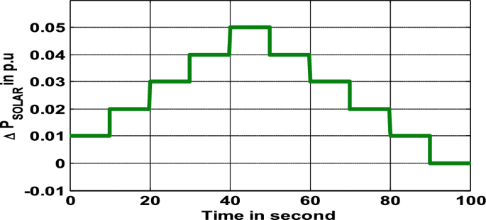
Time variant step load
Fig. 12 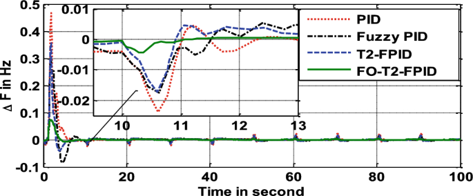
Frequency deviation under step load
-
D.
Frequency stability under the reflectance of \( \Delta P_{L} \), \( \Delta P_{W} \) and \( \Delta P_{\varPhi } \) simultaneously
This case study deals with the frequency regulation study of an EV based AC microgrid system under the effect of all three uncertainties (\( \Delta P_{L} \),\( \Delta P_{W} \) and \( \Delta P_{\varPhi } \)) simultaneously. The dynamic responses of all three uncertainties in simultaneous action are depicted in Fig. 13. The controlled dynamic response of system frequency under such disturbance is depicted in Fig. 14. The simulated frequency response due to FO-T2-FPID controller exhibits quicker settling time of 6.8 s with reduced peak overshoot of 0.08 Hz. The performance index parameters like settling time, peak overshoot and peak undershoot of frequency responses resulted under different controllers and uncertainties are gathered in Table 3. It has been noticed from Table 3 that for same I-GWO optimal scenario, the percentage improvement in settling time of ΔF (load uncertainty) and ΔF (solar power uncertainty) with FO-T2-FPID controller compared to T2-FPID are 5.70% and 39.72% and compared to Fuzzy PID are 96.25% and 142.50% respectively. Subjective analysis over frequency response and the numerical result suggests proposed I-GWO optimized FO-T2-FPID controller improves system performances significantly and exhibits superior performance over optimal T2-FPID, fuzzy PID and PID controllers.
Fig. 13 
Time variant step load
Fig. 14 
Frequency deviation under step load
Table 3 Performance index parameters of dynamic frequency response -
E.
Performance analysis under stochastic generated uncertainties
The uncertainties of load dynamics, wind power fluctuations and solar power variation are unpredictable and undergo with a continuous variation. In real-time validation, these uncertainties may be predicted under stochastic analysis. This section especially highlights on system performance under various stochastic generated uncertainties. The stochastically generated step load, wind power fluctuations and solar power variation are illustrated in Fig. 15, 16, 17, 18 and 19 respectively. The deviation in frequency response under stochastic generated load variation is depicted in Fig. 16. The response with FO-T2-FPID controller settles faster at 4.04 s and exhibits the least overshoot of 0.08 Hz as compared to other approaches. However, the responses of frequency deviation under wind power fluctuation and solar power variation are illustrated in Figs. 18 and 20 respectively. The dynamic frequency responses which have been resulted with FO-T2-FPID controller exhibit least settling time and also damp out the oscillation effectively as compared to responses under T2-FPID and fuzzy PID controllers. The magnify figure gracefully defend the superiority of FO-T2-FPID controller.
Fig. 15 
Time variant stochastic step load
Fig. 16 
Frequency deviation under stochastic load
Fig. 17 
Time variant stochastic wind power fluctuation
Fig. 18 
Frequency deviation under stochastic wind power
Fig. 19 
Time variant stochastic solar power variation
Fig. 20 
Frequency deviation under stochastic solar power
Critical analysis over all frequency responses confers supremacy of proposed I-GWO designed FO-T2-FPID controller in response to frequency control of an EV based AC microgrid system.
-
A.
-
II.
Technique stage
This stage deals with to defend the superiority of proposed I-GWO technique over grey wolf optimization (GWO) and particle swarm optimization (PSO) in regard to optimal design the proposed FO-T2-FPID controller. The optimal controller is suggested to obtain frequency stability in the EV based microgrid system under different disturbances such as load dynamics, wind power fluctuations and solar power regulations. The controlled response of deviation in microgrid frequency due to all techniques i.e. I-GWO, GWO and PSO optimized FO-T2-FPID controller under load uncertainty (\( \Delta P_{L} \)) is illustrated in Figs. 21 and 22. It is cleared from the response that proposed I-GWO optimized FO-T2-FPID controller develops least settling time (7.2 s) oriented response as compared to GWO and PSO. However, the controlled dynamic responses of frequency deviation under wind power uncertainty (\( \Delta P_{W} \)) and solar power uncertainty (\( \Delta P_{\varPhi } \)) are depicted in Figs. 24 and 26 respectively. The dynamic frequency responses obtained under I-GWO optimized FO-T2FPID controller exhibit faster settling time with least damping oscillations. The magnify figure clearly indicates the oscillation and settling time of responses and enough to validate the superiority of proposed I-GWO algorithm over GWO and PSO algorithms. The time-domain dynamic responses are resulted with proposing all techniques (I-GWO, GWO, PSO) based FO-T2-FPID controller. The performance index parameters such as settling time, peak overshoot and peak undershoot of all frequency responses depicted in Figs. 22, 23, 24, 25 and 26 are gathered in Table 4. The simulated convergence curve of all optimization techniques is illustrated in Fig. 27. The convergence curve suggests faster convergence ability of the proposed I-GWO algorithm with least ITAE value. The ITAE values of all optimal controllers are also represented graphically in Fig. 28 and defend the superiority of I-GWO algorithm to obtain improved ITAE values.
Fig. 21 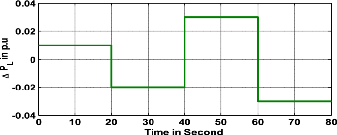
Time variant step load
Fig. 22 
Frequency deviation under step load
Fig. 23 
Time variant wind power fluctuation
Fig. 24 
Frequency deviation under wind power fluctuation
Fig. 25 
Time variant solar power variation
Fig. 26 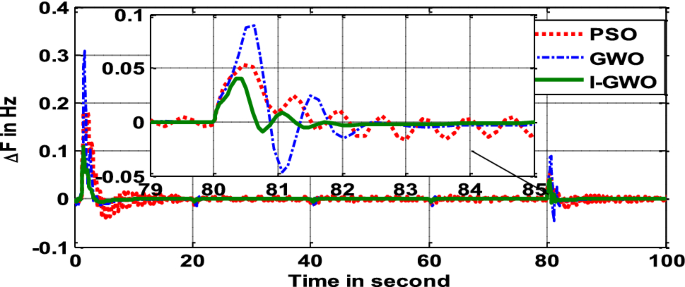
Frequency deviation under solar power variation
Table 4 Settling time, peak overshoot and peak undershoot of frequency response under different techniques Fig. 27 
Convergence Curve
Fig. 28 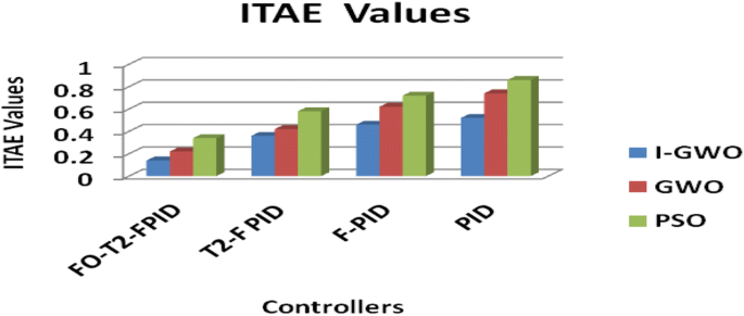
ITAE values of various optimization techniques
The numerical results addressed in Table 4 confer supremacy of proposed I-GWO algorithm to obtain the least settling time and reduced oscillations in the frequency response. Further, it is clearly visualised from Table 4 that for same controller structure the percentage improvement in settling time of frequency response resulted under all uncertainties ∆F (L + W + S) with I-GWO algorithm compared to GWO and PSO are 17.82% and 36.52% respectively. Overall analysis suggests the proposed I-GWO technique is found to be better for optimal designing various controllers in response to frequency regulation of an AC microgrid system.
-
III.
Sensitive analysis
The robustness of the proposed FO-T2-FPID controller is validated through different sensitive analysis. The sensitive analysis is progressed with wide regulation of system parameters such as variation in time constant of governor (\( T_{G} \)), turbine time constant (\( T_{d} \)), fuel cell time constant (\( T_{FC} \)), micro-turbine time constant (\( T_{MT} \)), electric vehicle time constant (\( T_{EV} \)), wind turbine time constant (\( T_{WIND} \)) and PV cell time constant (\( T_{PV} \)). In this research study, all these parameters are regulated with \( \pm 30\% \) from their nominal values to investigate system performance under the proposed FO-T2-FPID controller.
-
A.
Varying governor time constant (TG)
This case study presents dynamic behavior of the system frequency under regulation of diesel engine governor time constant (TG) with \( \pm 30\% \) from its nominal value. Under such conditions, the response of deviation in system frequency is depicted in Fig. 29. All three responses are resulted without changing the optimal parameters of the proposed FO-T2-FPID controller. It is clearly visualised from the frequency response that, under wide regulation of governor time constant it is not required to retune the controller parameters again to obtain a desired response in the existing system. The dynamic response suggests the proposed FO-T2-FPID controller is robust in nature.
Fig. 29 
Frequency deviation under regulation of TG
-
B.
Varying turbine time constant (Td)
This section has well addressed on sensitive analysis with wide regulation of diesel engine turbine time constant (Td). Unlike section ‘A’ the turbine time constant is varied \( \pm 30\% \) from its nominal value to investigate system performance under unchanged controller optimal parameters. The deviation in system frequency which has been resulted under wide regulation of Td is depicted in Fig. 30. The sensitive analysis of this research work has been progressed with the regulation of TFC, TEV, TMT, TWIND and TPV by \( \pm 30\% \) from their nominal values. The time-domain simulated frequency responses under such parametric regulations are illustrated in Figs. 29, 30, 31, 32, 33, 34, 35 and 36, respectively. The responses are simple overlapping or little deviation under wide regulation of system parameters. This suggests the wide regulation of system parameter has no impact over system performances under the presence of unchanged controller parameters. Critical analysis over all dynamic response confers to get desired performance, the controller parameters need not to be retuned again with wide variation of system parameters.
Fig. 30 
Frequency deviation under regulation of Td
Fig. 31 
Frequency deviation under regulation of TFC
Fig. 32 
Frequency deviation under regulation of TEV
Fig. 33 
Frequency deviation under regulation of TMT
Fig. 34 
Frequency deviation under regulation of TWIND
Fig. 35 
Frequency deviation under regulation of TPV
Fig. 36 
Sensitive analysis through bar graph
-
A.


The settling time and overshoot of frequency responses which have been obtained with wide regulation of various system parameters are gathered in Table 5. Thorough assessment over Table 5 shows the percentage variation in settling time of ∆F (under load uncertainty) at + 30% and − 30% with respect to normal loading are 0.82% and 1.96% respectively. The least percentage variation in settling time justifies robustness of proposed FO-T2-FPID controller. The numerical results such as settling time and peak overshoot are very close approximation under any parametric regulations. Numerical results and dynamic responses confer robustness of proposed FO-T2-FPID controller regarding frequency regulation of an AC microgrid system.
5.1 Comparison with recent frequency control approaches
A commonly used two equal area non-reheat power system (Ali and Abd-Elazim 2011; Rout et al. 2013; Panda et al. 2013; Panda and Yegireddy 2013; Sahu et al. 2015) is considered to validate the superiority of proposed I-GWO optimized FO-T2-FPID controller. To obtain controlled frequency response, each area of the system are allocated with identical FO-T2-FPID controller and the controller parameters are optimally designed with employing an I-GWO algorithm. The identical power system (Ali and Abd-Elazim 2011; Rout et al. 2013; Panda et al. 2013; Panda and Yegireddy 2013; Sahu et al. 2015) and suggested objective function (ITAE) are considered to make a critical comparison of proposed I-GWO based FO-T2-FPID approach over few reported approaches (Ali and Abd-Elazim 2011; Rout et al. 2013; Panda et al. 2013; Panda and Yegireddy 2013; Sahu et al. 2015). The I-GWO designed optimal parameters of proposed FO-T2-FPID controller are:
At time t = 0 s, an increased step load perturbation of 10% is realised in area1 to demonstrate the comparative performance of proposed I-GWO: FO-T2-FPID controller over other reported approaches such as GA: PI, ZN: PI, BFOA: PI (Ali and Abd-Elazim 2011), DE: PI (Rout et al. 2013), Hybrid BFOA-PSO: PI (Panda et al. 2013), NSGA-II: PI, NSGA-II: PIDF (Panda and Yegireddy 2013), PS: fuzzy PI, PSO: fuzzy PI (Panda and Yegireddy 2013), Hybrid PSO-PS: Fuzzy PI (Sahu et al. 2015).
Under different frequency control approach, the deviation in the frequency response of area 1 is illustrated in Fig. 37. It is clearly visualised from the frequency response that proposed I-GWO designed FO-T2-FPID controller develops improved frequency response with least settling time of 3.20 s and reduced peak undershoot of 0.0134 Hz. The performance index parameters like settling time, peak overshoot and peak undershoot of resulted frequency response under all approaches along with respective ITAE values are assembled in Table 6. It has been conferred from Table 6 that proposed I-GWO designed FO-T2-FPID controller is able to obtain improved system performance with minimum ITAE value, least settling time, reduced peak overshoot and undershoot as compared to other reported approaches.

Deviation in frequency of area 1 under various AGC approaches
6 Conclusions
In this paper, an I-GWO based FO-T2-FPID controller is recommended for frequency regulation of an EV based AC microgrid. The microgrid dynamic performances are investigated under various uncertainties like load dynamics, wind power fluctuation and variation in solar irradiation power. The proposed FO-T2-FPID controller is found to be better to regulate frequency in an islanded AC microgrid system under plugin electric vehicle and various uncertainties. The superiority I-GWO based FO-T2-FPID controller is established by evaluating the results for the same test system with some recent publications. It is observed that the I-GWO based FO-T2-FPID approach offers considerably superior results in terms of error values, settling times and peak under/overshoots compared to PSO and GWO based FO-T2-FPID controllers. It is noticed that for same I-GWO method, the percentage improvement in ITAE value by I-GWO based FO-T2-FPID controller compared to T2-FPID, F-PID and PID controller are 42.86%, 100% and 114.28% respectively. Therefore it can be concluded that I-GWO based FO-T2-FPID controller outperforms T2-FPID, F-PID and PID controller in response to frequency regulation of the microgrid system. It is noticed that for the same FO-T2-FPID structure the percentage improvement in settling time of ΔF (load uncertainty) and ΔF (wind uncertainty) with I-GWO algorithm compared to PSO are 37.85% and 31.22% and compared to GWO are 19.32% and 15.60%. A sensitivity study is carried out with parameter variations and random pulse variation. It is noticed that suggested FO-T2-FPID is robust and achieves better performance under changing type, size, location of load disturbance and system elements.
References
Alharbi T, Bhattacharya K, Kazerani M (2019) Planning and operation of isolated microgrids based on repurposed electric vehicle batteries. IEEE Trans Ind Inf 15(7):4319–4331
Ali ES, Abd-Elazim SM (2011) Bacteria foraging optimization algorithm based load frequency controller for interconnected power system. Int J Electr Power Energy Syst 33(3):633–638
Arghandeh R, Pipattanasomporn M, Rahman S (2012) Flywheel energy storage systems for ride-through applications in a facility microgrid. IEEE Trans Smart Grid 3(4):1955–1962
Bagal HA, Soltanabad YN, Dadjuo M, Wakil K, Ghadimi N (2018) Risk-assessment of photovoltaic-wind-battery-grid based large industrial consumer using information gap decision theory. Sol Energy 169:343
Bahmani-Firouzi B, Azizipanah-Abarghooee R (2014) Optimal sizing of battery energy storage for micro-grid operation management using a new improved bat algorithm. Int J Electr Power Energy Syst 56:42–54
Bevrani H, François B, Ise T (2017) Microgrid dynamics and control. Wiley, New York
Chen M-R, Zeng G-Q, Dai Y-X, Kang-Di L, Bi D-Q (2019) Fractional-order model predictive frequency control of an islanded microgrid. Energies 12(1):84
Enrico S, Kai D (2016) Fractional calculus: models and numerical methods, vol 5. World Scientific, Singapore
Gao W, Darvishan A, Toghani M, Mohammadi M, Abedinia O, Ghadimi N (2019) Different states of multi-block based forecast engine for price and load prediction. Int J Electr Power Energy Syst 104:423–435
Ghadimi N, Akbarimajd A, Shayeghi H, Abedinia O (2018) Two stage forecast engine with feature selection technique and improved meta-heuristic algorithm for electricity load forecasting. Energy 161:130–142
Hemmati M, Abapour M, Mohammadi-Ivatloo B (2020) Optimal scheduling of smart microgrid in presence of battery swapping station of electrical vehicles. In Electric vehicles in energy systems. Springer, Cham, pp 249–267
Kennedy RP, Ravindra MK (1984) Seismic fragilities for nuclear power plant risk studies. Nucl Eng Des 79(1):47–68
Khodaei H, Hajiali M, Darvishan A, Sepehr M, Ghadimi N (2018) Fuzzy-based heat and power hub models for cost-emission operation of an industrial consumer using compromise programming. Appl Therm Eng 137:395–405
Kishor N, Saini RP, Singh SP (2007) A review on hydropower plant models and control. Renew Sustain Energy Rev 11(5):776–796
Mehri S, Shafie-Khah M, Siano P, Moallem M, Mokhtari M, Catalão JPS (2017) Contribution of tidal power generation system for damping inter-area oscillation. Energy Convers Manag 132:136–146
Mirjalili S, Mirjalili SM, Lewis A (2014) Grey wolf optimizer. Adv Eng Softw 69:46–61
Mishra D, Sahu PC, Prusty RC (2019) Tidal energy integrated robust frequency control of an islanded AC microgrid with improved-MFO tuned tilt controller. Int J Innov Technol Explor Eng
Mohamed EA, Mitani Y (2019) Load frequency control enhancement of islanded micro-grid considering high wind power penetration using superconducting magnetic energy storage and optimal controller. Wind Eng 43(6):609–624
Mohammadi S, Soleymani S, Mozafari B (2014) Scenario-based stochastic operation management of microgrid including wind, photovoltaic, micro-turbine, fuel cell and energy storage devices. Int J Electr Power Energy Syst 54:525–535
Pan I, Das S (2015) Fractional order AGC for distributed energy resources using robust optimization. IEEE Trans Smart Grid 7(5):2175–2186
Panda S, Yegireddy NK (2013) Automatic generation control of multi-area power system using multi-objective non-dominated sorting genetic algorithm-II. Int J Electr Power Energy Syst 53:54–63
Panda S, Mohanty B, Hota PK (2013) Hybrid BFOA–PSO algorithm for automatic generation control of linear and nonlinear interconnected power systems. Appl Soft Comput 13(12):4718–4730
Podlubny I, Dorcak L, Kostial I (1997) On fractional derivatives, fractional-order dynamic systems and PI/sup/spl lambda//D/sup/spl mu//-controllers. In: Proceedings of the 36th IEEE conference on decision and control (vol. 5, pp 4985–4990). IEEE
Porwal M, Parmar G, Bhatt R (2018) Robustness analysis of GWO/PID approach in control of ball hoop system with ITAE objective function. Int J Comput Sci Eng 6(8):218–222
Regulagadda P, Dincer I, Naterer GF (2010) Exergy analysis of a thermal power plant with measured boiler and turbine losses. Appl Therm Eng 30(8–9):970–976
Rout UK, Sahu RK, Panda S (2013) Design and analysis of differential evolution algorithm based automatic generation control for interconnected power system. Ain Shams Eng J 4(3):409–421
Saeedi M, Moradi M, Hosseini M, Emamifar A, Ghadimi N (2019) Robust optimization based optimal chiller loading under cooling demand uncertainty. Appl Therm Eng 148:1081–1091
Sahu PC, Prusty RC (2019) Robust frequency control of an islanded AC micro grid using BDA optimized 3DOF controller under plug in electric vehicle. Int J Eng Adv Technol
Sahu RK, Panda S, Sekhar GC (2015) A novel hybrid PSO-PS optimized fuzzy PI controller for AGC in multi area interconnected power systems. Int J Electr Power Energy Syst 64:880–893
Sahu PC, Prusty RC, Panda S (2017) ALO optimized NCTF controller in multi area AGC system integrated with WECS based DFIG system. In: 2017 International conference on circuit, power and computing technologies (ICCPCT) (pp 1–6). IEEE
Sahu PC, Mishra S, Prusty RC, Panda S (2018) Improved-salp swarm optimized type-II fuzzy controller in load frequency control of multi area islanded AC microgrid. Sustain Energy Grids Netw 16:380–392
Sahu PC, Prusty RC, Panda S (2019a) Stability analysis in RECS-integrated multi-area AGC system with SOS algorithm based fuzzy controller. In Computational intelligence in data mining. Springer, Singapore, pp 225–235
Sahu PC, Prusty RC, Panda S (2019b) Approaching hybridized GWO-SCA based type-II fuzzy controller in AGC of diverse energy source multi area power system. J King Saud Univ Eng Sci 32:186
Sedghi L, Fakharian A (2017) Voltage and frequency control of an islanded microgrid through robust control method and fuzzy droop technique. In: 2017 5th Iranian joint congress on fuzzy and intelligent systems (CFIS) (pp 110–115). IEEE
Sivalingam R, Chinnamuthu S, Dash SS (2017) A modified whale optimization algorithm-based adaptive fuzzy logic PID controller for load frequency control of autonomous power generation systems. Automatika 58(4):410–421
Yin C, Wu H, Locment F, Sechilariu M (2017) Energy management of DC microgrid based on photovoltaic combined with diesel generator and supercapacitor. Energy Convers Manag 132:14–27
Author information
Authors and Affiliations
Corresponding author
Additional information
Publisher's Note
Springer Nature remains neutral with regard to jurisdictional claims in published maps and institutional affiliations.
Appendix
Appendix
D = Coefficient of damping = 0012 (pu/Hz); M = Constant for Inertia = 0.2 (pu/s);TFC = Time constant (TC) of fuel cell (FC) = 4 s; KFC = Gain of FC = 1/5; TBES = TC of battery = 0.1 s; KBES = Gain of battery = 1/300; TFES = TC of flywheel energy storage(FES) = 0.1 s; KFES = Gain of FES = 1/100; Td = TC of Diesel engine generator(DEG) = 2 s; TMT = TC of micro-turbine (MT) = 2 s; KMT = Gain of MT = 1; TWTG = TC of wind turbine generator (WTG) = 1.5 s; KWTG = Gain of WTG = 1; TPV = TC of photo voltaic (PV) cell = 1.8 s;KPV = Gain of PV = 1; TEV = TC of Electric Vehicle (EV) = 0.2 s; KEV = Gain of EV = 1/100; TAE = TC of aqua electrolyser (AE) = 0.5 s; KAE = Gain of AE = 1/25; R = System regulation = 2.4 Hz/Mw
Rights and permissions
About this article

Cite this article
Sahu, P.C., Prusty, R.C. & Panda, S. Improved-GWO designed FO based type-II fuzzy controller for frequency awareness of an AC microgrid under plug in electric vehicle. J Ambient Intell Human Comput 12, 1879–1896 (2021). https://doi.org/10.1007/s12652-020-02260-z
Received:
Accepted:
Published:
Issue Date:
DOI: https://doi.org/10.1007/s12652-020-02260-z