Allomorphy without context specification: a case study of Czech adjectival stems

Abstract

This paper investigates stem-marker allomorphy in Czech adjectives. It shows that an analysis based on the frequently used context-sensitive rules comes at the expense of having to postulate widespread accidental homophony or disjunctive rules. The paper further demonstrates that the allomorphy can be accounted for within an approach based on portmanteau realisation of features, specifically the version of Nanosyntax proposed in Starke (2018), although alternative implementations are conceivable. Along the way, we explore a fine-grained decomposition of adjectival meaning and we also discuss the implications of these observations for the general issues surrounding context-sensitive rules compared to other systems of dealing with allomorphy.

1 Introduction

In Czech, there is a sizeable class of adjectives, which, morphologically speaking, correspond to a root directly followed by agreement. An example is in (1).

• (1) mlad- ý

  young agr

  ‘young’

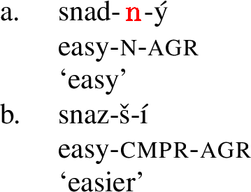
Another large class of adjectives has a special marker , which occurs between the root and the agreement marker, as in (2).¹ We sometimes refer to this morpheme as an ‘augment.’

• (2) snad- - ý

  easy- n agr

  ‘easy’

The reasons for analysing in (2) and elsewhere as an independent morpheme are the following. First of all, some (though not all) roots that require exist independently of the stem marker, see, for instance, (3).

• (3)

  

Secondly, the stem marker is sometimes absent in the comparative, as in (4):

• (4)

  

Another indication of the morphemic status of is the sheer number of adjectives whose stem ends in . Table 1 provides a representative (even if not exhaustive) list of adjectives in the two classes. The size of the table indicates that both classes are relatively well represented in Czech. The zero class appears to be slightly less numerous than the class: the list of adjectives in the class is near exhaustive, while more adjectives could easily be added to the list of the adjectives.²

Table 1 The two classes of adjectives (Ø vs. n)

The morphological complexity of adjectives with the stem marker suggests a structure for the positive degree with at least two underlying positions, as in (5a). In the tree, there is a root position lexicalized by snad ‘easy’ and a position labelled little a (an adjectivizing head) lexicalized by the morpheme.

• (5)

  

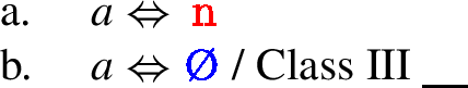
If the structure (5a) is adopted, then, for the adjectives that do not take an augment, one could argue that a is lexicalized by a zero morpheme, as in (5b). The proposals in (5) ultimately boil down to the idea that we are dealing with two allomorphs of little a, as in (6).

• (6)

  

This article compares two approaches to the allomorphy in (6). One makes use of context-sensitive rules, while the other one is based on portmanteau lexicalisation. Let us sketch the two alternatives below.

Under the context-sensitive approach (see amongst others Siegel, 1977; Halle & Marantz, 1993; Moskal & Smith, 2016; Choi & Harley, 2019), one would specify the stem marker as a context-free realisation of little a (based on the fact that adjectives with are more numerous), while would appear in the context of a restricted set of roots, namely those in the left-hand column in Table 1.

• (7)

  

An alternative way of depicting this proposal is in (8): the idea is that depending on which specific root lexicalises the $\sqrt{ \phantom{...} }$ position, a particular adjectival marker appears ( or ). The two markers are not distinguished in terms of the features that they realise, but purely by context.

• (8)

The second possible analysis is phrased in terms of portmanteau lexicalisation (see McCawley, 1968; Halle & Marantz, 1993; Williams, 2003; Chung, 2007; Neeleman & Szendroi, 2007; Radkevich, 2010). In this analysis, the root of the adjectives of the class lexicalises two heads at the same time, that of the root and the little a, as shown in (9a).

• (9)

  

In this approach, there is no zero morpheme : the absence of arises simply as a result of the fact that there is no need to lexicalise little a with roots that are capable of doing this on their own, as shown on the second line of (10).

• (10)

On this approach, the stem marker is the only marker lexicalising little a, and it appears with all roots that fail to lexicalise this head, as on the first row in (10).

This article shows that these are not equivalent analyses, as also discussed in Embick and Marantz (2008), Bobaljik (2012, 146-152), Banerjee (2021a,b) and Caha (to appear). This paper contributes to this debate by pointing out that the portmanteau analysis in (10) is capable of describing patterns of stem distribution in an elegant and straightforward manner, while a theory based on context-sensitive rules must postulate a proliferation of accidentally homophonous lexical entries, or disjunctive specifications.

The specific pattern demonstrating the advantage of the portmanteau approach concerns the distribution of the stem markers in the positive and the comparative. Specifically, not all adjectives that have the stem marker in the positive also have it in the comparative, and vice versa. In total, four different root classes can be distinguished based on whether they have or zero in the positive and the comparative, as depicted in Table 2.³

Table 2 Four different root classes

As we can see, Class I roots have both in the positive and in the comparative. Class II roots have only in the comparative. Class IV roots have only in the positive degree. Finally, Class III roots do not have in any of the two forms.

The main goal in this paper is to establish the empirical pattern and show that if context-sensitive rules are used, the distribution of stem markers as in Table 2 can only be described if one invokes multiple accidentally homophonous lexical entries. In contrast, the same pattern can be straightforwardly modelled within the portmanteau approach, relying on the Nanosyntax model of lexicalisation as proposed in Starke (2018).

The paper is organised as follows. In Sect. 2, we describe the distribution of the stem markers and in the positive. Section 3 turns to the comparative, and Sect. 4 discusses the shortcomings of context-sensitive rules. In Sect. 5, we establish our assumptions regarding the structure of the positive and comparative degrees. In Sect. 6, we present the portmanteau analysis of classes I-III, and Sect. 7 shows how the distribution of stems in Class IV can be captured. Section 8 describes the Nanosyntactic derivations in detail, and Sect. 9 concludes.

2 The positive

This section discusses the possible reasons why certain roots appear with the stem marker while other roots appear with no overt stem marker (). We show that the presence/absence of the stem marker cannot be determined by inspecting the phonology or the meaning of the root. The quality of the stem marker also cannot be predicted from the morphological category of the base. We therefore conclude that the selection between the root and the stem marker is governed by an arbitrary lexical class of the root.

We begin by showing that the choice between and is not governed by phonology. The reason is that many adjectives with phonologically similar roots belong in different classes. We have used one such example in (1) and (2) (with the roots mlad and snad), and many similar cases can be found in Table 1. The strongest case can be provided by a pair of homophonous adjectival roots meaning ‘left’ and ‘cheap.’ These different morphemes happen to have the same phonology, namely lev-. Yet, one of them (the one meaning ‘left’) lacks the augment (11a), while the other root with the meaning ‘cheap’ requires it (11b).

• (11)

  

The point is that it cannot be determined by looking at the phonology of the root (i.e., lev-) whether the root will be followed by or .⁴

An analogous point can be made about the meaning of the root, namely, it cannot be determined by considering the meaning alone whether the root is going to combine with or -. Thus, there are near synonymous roots like hrub- and drs-, both meaning ‘rough,’ with one of them combining with , see (12a), and the other with , see (12b).

• (12)

  

The difficulty to find some consistent common meaning across all the roots in either of the classes can be further verified by inspecting Table 1.

Finally, the quality of the stem marker cannot be predicted from the morphological category of the base. Thus, one cannot say that is found with nominal roots, while is found with adjectival roots. We now demonstrate the perils of such an approach on a couple of examples.

To begin with, it does seem to be the case that a number of adjectives with may be considered denominal. For example, the adjective čest--ý ‘honest’ has a related noun čest ‘honour,’ and may thus be considered a denominal adjective, see (13) (also compare the case of jas ‘light’ in (3) above).

• (13)

  

However, not all adjectives with are denominal. For example, the root of the adjective skrom--ý ‘modest’ cannot be used without the augment at all, as illustrated in (15).⁵

• (14)

  

Thus, it cannot be concluded that the morphological category of the root (nominal vs. not) allows one to uniquely determine what kind of stem marker will be found in the adjectival use of a root.

The same can be demonstrated by the following pair of examples. The example (15) shows that the noun stříbr-o ‘silver’ has a corresponding color/material adjective in :

• (15)

  

However, the same type of adjective derived from the noun zlat-o ‘gold’ lacks , despite the fact that the noun appears rather similar to stříbr-o in its semantics and morphological structure (both are neuter nouns belonging in the same declension). This is shown in (16).⁶

• (16)

  

We conclude from this that neither phonology, nor semantics, or the morphological category of the root allows speakers to predict what kind of stem marker will be used in the adjectival form of a root. Therefore, we shall treat the quality of the stem marker as an arbitrary (lexical) property of the root. This arbitrary nature of the pairing between the root and the stem marker fits well with both of the possible accounts sketched in Sect. 1. On both accounts, which stem a root has ( vs. ) is an arbitrary property of a lexical entry. On the contextual approach, this is due to an arbitrary lexical specification of the context of insertion. On the portmanteau approach, the arbitrariness of selection translates into the arbitrariness of lexical storage as well: some roots are stored as capable of lexicalising a, while other roots are unable to do so.

3 The comparative

This section discusses the distributional pattern of the stem-marker in the comparative, which was already mentioned in Sect. 2, and which is repeated here in Table 3.

Table 3 Four different root classes

The main observation is that each of the two stem classes we discussed for positive degree adjectives may have or lack the stem-marker in the comparative. As a result, each class is further subdivided into two subclasses depending on the quality of the stem marker in the comparative. Classes I and II have the stem-marker in the comparative, but differ in that Class I has in the positive, while Class II has . Classes III and IV have in the comparative, but differ in that Class IV has in the positive, while Class III has .

The table shows that for a given adjective, the presence or absence of is not only determined by the left context, i.e., by a particular root, but also by the right context, i.e., whether the stem is followed by a comparative marker or not. In some classes, the presence of the comparative makes disappear (in Class IV), other times, only appears in the comparative (in Class II). In Classes I and III, the stem marker (whether or ) is unaffected by the degree.

Let us now illustrate these patterns with examples. To present them clearly, let us first mention that in Czech, the comparative itself has two allomorphs: š and ějš (Křivan, 2012). Their distribution is once again arbitrarily determined by the root. We illustrate the arbitrary nature in Table 4, where two roots that are similar in their phonology and meaning each combine with a different allomorph.

Table 4 Two allomorphs for cmpr

In our analysis of these patterns in Sect. 5, we shall adopt the analysis by Caha et al. (2019) and analyse ějš as a sequence of two morphemes, namely ěj and š. The reason for proposing the decomposition is that both allomorphs share an identical piece, namely š, and that these two pieces lead an independent life. In Table 4, it has been already noted that in the comparative of certain adjectives, only š appears while ěj is absent. In addition, comparative adverbs of adjectives in ěj-š, like chab ‘weak’ (17a), have the form ěj-i, with ěj present and š absent, (17b).

• (17)

  

In our description, we will not dwell on this decomposition, but we come back to it later in Sect. 5.

Since the allomorphy between š and ějš is determined arbitrarily by the base to which they attach, we could expect that each of the Classes I-IV in Table 3 could have two subclasses, depending on whether the comparative has š or ějš. In reality, the situation is simpler in that when the comparative adjective has the stem marker , then the comparative is always ějš. This is a result of the fact that (in a local fashion) controls the allomorphy of the comparative, and so only one comparative allomorph is allowed in Classes I and II. However, when is absent in the comparative, we find both allomorphs, with their distribution determined by the root. As a result, Classes III and IV as given in Table 3 divide even further into two additional subclasses, depending on the allomorph of the comparative.

With the background in place, consider Table 5, which depicts all the relevant classes as described up to now.⁷

Table 5 The distribution of and in the positive and the comparative

We can see that in Classes III and IV, where the comparative morpheme directly follows the root, we find two different sub-classes as a function of the š ∼ ěj-š allomorphy. In all comparatives, the final vowel í is the nom.sg agreement marker.

The most important thing for our theoretical claims about allomorphy is the existence of Classes I-IV, and the fact that these are arbitrary morphological classes. We have discussed the arbitrary nature of the stem difference ( vs. ) for the positive. Now we discuss the same issues for the comparative.

The first thing to know is that the absolute majority of adjectives belong in Classes I and III. Thus, for most adjectives, the issue of whether or not an adjective has or in the comparative reduces to the issue of what stem marker there is in the positive. Since this on its own is a matter of arbitrary class membership, we must conclude that the difference between vs. in the comparative is also a matter of arbitrary class membership.

Against this background, let us discuss the minority Classes II and IV, which change the class marker between the positive and the comparative. Let us first discuss Class IV, which loses the stem marker in the comparative. We will be looking at this class side by side with Class I, which has the stem marker both in the positive and in the comparative. The question is whether it can be somehow predicted by looking at the positive alone which adjective is going to keep in the comparative, and which is not. Leaving aside the fact that there are only few adjectives that lack in the comparative, the answer seems to be that the loss of is unpredictable.

In Table 6 we provide two examples of adjectives with a comparative in š. Note that when the comparative š attaches to the root without an intervening , there is a consonant mutation from d to z (a process attested elsewhere in the language).

Table 6 Adjectives with cmpr in š that may lose in cmpr

As the data show, leaving out with these roots is optional, rather than obligatory, i.e. they can belong either to Class I or to Class IV.⁸ Still, the possibility to omit - contrasts with adjectives that are phonologically and/or semantically analogous, and where dropping the is absolutely impossible, see Table 7. These adjectives unambiguously belong in Class I.

Table 7 Adjectives that keep in cmpr

In sum, the majority pattern is one where adjectives keep the stem marker as we go from the positive to the comparative (Class I). However, there are a few adjectives that allow for to be missing (Class IV). As to which adjectives these are is not predictable, and must be memorised on a case by case basis.

The situation is similar with the adjectives that take the ějš allomorph of the comparative. Here some adjectives also optionally drop and, when this happens, they exhibit Class IV pattern. An example of such an adjective is provided in Table 8. As said, preserving the seems to be an option, although dropping it is strongly preferred. The corpus data from Křivan (2012) indicate that the ratio is approximately 270:1 in favour of Class IV behaviour, i.e. in favour of dropping the stem marker . To a native speaker, the comparative that preserves the also sounds decidedly worse.

Table 8 optional drop with ějš cmpr

The adjectives in Table 9 display only Class I behaviour. They show that the reason for dropping the in Table 8 is not phonological in some obvious sense, since phonologically similar roots maintain it. We therefore proceed under the assumption that the presence vs. absence of in various positive and comparative forms is to be treated as allomorphy triggered by arbitrary morphological classes.

Table 9 retention with ějš cmpr

Let us now turn to the other minority class, Class II, which we consider alongside Class III. Both classes lack the stem marker in the positive. The overwhelming majority of such adjectives also lacks in the comparative, forming what we call Class III. However, there are a few adjectives that require in the comparative. All of these adjectives have something in common. Specifically, Křivan (2012, 40) points out that all Class II adjectives are homophonous with present participles in c (roughly analogous to English ing). While this restriction is interesting, our main point is going to be that the specific adjectives that belong in this class are still unpredictable. (Put simply, not all adjectival participles pattern like this.)

Let us begin the discussion of Class II by pointing out that the restriction to present participles is indeed morphological, rather than phonological: it does not concern the sound corresponding to the grapheme c, i.e. [ʦ], but the morpheme c in its capacity as a participial marker. Thus, when an adjectival base ends in the sound c that is not a participial marker, then is found both in the positive and in the comparative. This is illustrated in Table 10 for the root prac ‘work,’ and for the bound root vzác ‘rare.’

Table 10 Adjectives with roots ending in c that take

The point of presenting the adjectives in Table 10 is to show that there is nothing phonologically wrong about having the stem marker follow a c-final base in the positive. Yet this is impossible for Class II adjectives like ‘desirable,’ which must have in the positive, and in the comparative, as is shown in Table 11.

Table 11 Class II adjective in c

Having determined that we are dealing with a morphological class rather than a phonological class, let us zoom in on the adjectival present participles. Our main point is that even in this small niche, ‘predictability’ of behaviour is severely restricted. In other words, while it is the case that only adjectival present participles exhibit this pattern, it is not the case that all adjectival present participles exhibit the relevant pattern.

For instance, the present participle vroucí, derived from the verb vřít ‘to boil,’ has an idiomatic reading ‘heartfelt’, and can be graded in this reading, see Table 12. When the comparative is formed, the stem marker appears.

Table 12 The adjectival present participle of vřít ‘boil’

However, most participles do not accept any form of suffixal comparative marking. We illustrate this in Table 13 on the participle derived from the verb šokovat ‘to shock,’ see Table 13. This participle has an adjectival reading because it can be preceded by ‘very’ (Wasow, 1977); see the second column in Table 13. However, despite being adjectival, the participle ‘shocking’ does not accept any comparative suffixes, whether with or without it.

Table 13 The adjectival present participle of šokovat ‘shock’

We thus conclude that membership in Class II is subject to lexical idiosyncrasy, rather than predictable on the basis of information that is independently available when the positive degree is inspected. Therefore, what we need is a theory of how each adjectival base combines with the stem marker ( vs. ) in a given degree construction. These selectional requirements must be sensitive to the identity of a specific root/base, rather than valid for all adjectives across the board.

Before we look into the details of how this works, we again note that context-sensitive rules and portmanteau lexical entries are (in general terms) appropriate devices for the task, because they indeed involve stipulations over the content of specific lexical items (in the portmanteau approach) or stipulations over the sensitivity to other lexical items (contextual allomorphy). However, as we now proceed to show, context-sensitive rules cannot capture the distribution of and without postulating multiple instances of accidental homophony, while the portmanteau approach can.

4 Context-sensitive rules

This section shows that in an approach based on context-sensitive rules, the distribution of stems in Table 5 (repeated here as Table 14 for convenience) necessarily leads to a proliferation of accidental homophony or disjunctive context specification.

Table 14 The distribution of and in the positive and the comparative

The first step on this path is to adopt a specific structure for comparatives. In the seminal work on comparatives by Bobaljik (2012), it has been proposed that the structure of the comparative contains that of the positive (see also Smith et al., 2019). This is depicted in (18), where the comparative structure in (18b) adds an additional cmpr head on top of the positive, which is in (18a).

• (18)

  

With the structures in place, let us come back to the Vocabulary Items (VIs) needed to get the correct realisation of the little a head. Recall from (7) that the initial strategy was to say that is the default realisation of little a, see (19a).

• (19)

  

The effect of this context-free rule is that it inserts the stem marker after every root, unless counteracted by more specific VIs. The VI that we originally used to restrict its application was the one in (19b). Due to its context specification, this is a more specific VI and it therefore wins over the more general one, realising little a as zero in the context of Class III roots. These two VIs, taken together, correctly model the pattern found in Classes I and III in Table 14.

Let us now consider how we can extend or modify this set of VIs to account for the newly discovered Classes II and IV. The issue is that as the VIs currently stand in (19), we expect realisation of little a only in Class III, and in all other contexts. For Classes II and IV, this is correct only partially. For example, in Class IV, we see only in the positive, but not in the comparative.

To prevent from appearing in the comparative of Class IV, we need to have a VI that applies in this environment and realises little a as , thereby blocking the insertion of . The VI in question is given in (20).

• (20)

  

This VI competes with the two VIs in (19), and they jointly deliver a pattern as observed in Class IV, with the default realisation of little a in the positive, and a realisation in the comparative.

However, the cost to pay is that we have introduced accidental homophony into the system: we now have two different VIs inserting the same exponent , namely (19b) and (20). It is meaningless to simply unify the two VIs introducing by saying that is inserted either in the context of Class III roots or in the comparative of Class IV roots, since the VI thus created would have to be specified for a disjunction of environments. As Christopoulos and Zompí (2023, 11) put it in their recent work, specifying a single rule for a disjunctive context has exactly the same effect as accidental homophony. In doing so, ‘…admitting [disjunctive] rules […] (without anything else restricting possible disjunctions) opens the door to describing any type of exponent distribution under any theory of features by simply listing the contexts in which each exponent appears.’

To summarise, the distribution of stem markers in Class IV is problematic for context-sensitive rules, since these rules cannot capture it without invoking accidental homophony, or VIs with disjunctive context specifications (which basically amounts to the same thing).

The distribution of stem markers in Class II is problematic in the same way. Based on the rules in (19), we again expect to see both in the positive and in the comparative, since there is nothing blocking the application of the elsewhere rule (19a). However, empirically, we only find in the comparative of Class II.

In order to prevent the context-free from realising little a in the positive degree of Class II adjectives, we need to postulate a VI that only applies in the positive degree of this class. A VI like this is given in (21).

• (21)

  

This VI introduces yet another instance of accidental homophony, since, once again, the exponent is . However, the VI is problematic in yet another respect, namely the fact that it is triggered by a negative condition. Allowing negative specifications of contexts is again subject to the criticism voiced by Christopoulos and Zompí (2023) that it allows any kind of distribution of exponents. An anonymous reviewer further points out that it is doubtful whether negative conditions may serve as a trigger for a rule, as they are more reminiscent of a filter on the output of a grammar.

Before we leave this section, it is worth pointing out that the very same issues arise if we consider to be the default exponent, as in (22a). In this setting, the will appear in any environment where it is not blocked by a more specific VI. Once again, the problem is that the set of environments where does not appear is a disjunctive set of environments, which means we must have several different VIs for what looks like a single marker, namely . As in the scenario where is the default marker, we end up with three accidentally homophonous VIs, as shown in (22). For good measure, we also repeat the VIs needed for the first scenario, where is the default, in (23).

• (22)

  

• (23)

  

Summarising, the pattern of distribution observed for the stem markers and cannot be captured by context-sensitive rules without a proliferation of accidentally homophonous morphemes. It also requires negative specifications, i.e., the conditioning of rule application by the absence of specific features. In the remainder of this article, we show that if we adopt the Nanosyntax model of phrasal lexicalisation, the distribution of the stem markers can be captured without invoking either accidental homophony or negative specifications.

5 Setting up the features

The main idea behind the portmanteau account is that roots, stored in the post-syntactic lexicon, may be lexically associated to constituents of different sizes. For example, considering the simple structures in (24), we can have a set of roots that is lexically specified as lexicalising just the root node (24a), while other roots are associated to a larger constituent, and may lexicalise all the features of the positive, as in (24b).

• (24)

  

The interest of the analysis (24) is that the root controls the allomorphy between and without the need for any contextual specification. When the root lexicalises little a, there simply is no need to realise it for the second time by . Another interesting consequence is that this analysis requires no dedicated morpheme since the absence of is due to phrasal lexicalisation. As a result, the conundrum of how to set up the distribution of this morpheme using context-sensitive rules simply never arises.

In developing the analysis, we shall adopt a higher resolution decomposition of the positive and the comparative degrees than the one we have assumed so far. In (25a), we depict the structure of the positive. In this proposal, the positive decomposes into three features, dim, dir and point (see Vanden Wyngaerd et al., 2020).

• (25)

  

The features inside dirP (dir and dim) represent within syntax the scale underlying the semantics of gradable adjectives, sometimes referred to also as the measure function (see, e.g., Kennedy, 1999). The features dim and dir represent two independent components of each adjectival scale, namely its dimension and direction. The dimension corresponds to some domain of measurement, like velocity or size. The direction encodes the ordering of the values of a particular dimension. The direction can be positive or negative, distinguishing antonymous adjectives that share the same dimension, e.g., fast vs. slow, or tall vs. short.⁹

The feature point represents a point on the scale that the argument of the adjective must exceed. In the positive degree, the placement of this point is contextually given, and represents the standard according to which the adjective is evaluated. The picture in (26) shows the step-wise composition: dim and dir give us the scale in (26a), the projection point introduces a point (the standard) that the argument of the adjective must exceed (26b).

• (26)

  

As mentioned, in the absence of any specific instructions where the point is to be placed, its position is determined by context. This accounts for the fact that in the positive degree, the standard is context-dependent: who or what counts as fast or smart depends on the comparison class. With certain classes of adjectives (the so-called minumum-standard adjectives), the point coincides with the zero point on the scale (Kennedy & McNally, 2005). With such adjectives, it is enough that the argument of the adjective exceeds this zero standard for the positive degree to hold. For example, for a door to count as open, it is enough for it to attain a non-zero degree of openness. Similarly for the adjective wet: for a chair to count as wet, a non-zero degree of wetness is enough.

Let us now move to the structure of the comparative in (25b). As is obvious, our analysis of the comparative inherits from Bobaljik (2012) the idea that the structure of the positive is contained inside the comparative. At the same time, our structure differs from Bobaljik’s in that it has three comparative heads, rather than just one.¹⁰

The most immediate reason for us to propose the existence of three comparative heads are the Class II adjectives, where the comparative has three extra morphemes compared to the positive (they are placed inside the rectangle):

• (27)

  

Thus, in order to accommodate the three extra morphemes, we propose three extra heads. As far as their semantics is concerned, we think that the best way to make sense of them is to adopt the idea by Kennedy and Levin (2008), who propose that comparatives involve the construction of a new scale, which is derived from the one of the positive degree. If this is so, then the heads C0-C1-C2 essentially construct a new scale with the three relevant parameters of dimension, direction and point.¹¹

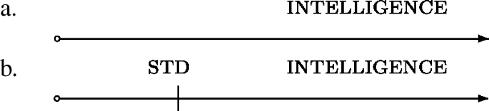
This idea is informally depicted in (28), with (28a) showing the scale of intelligence (dir+dim). Then a point is placed on the scale, see (28b). Unlike in the positive, the position of the point in the comparative is not determined by the context, but by the than-phrase. For instance, in an example like smarter than John, the point in (28b) represents the degree to which John is smart.

• (28)

  

Once the position of the point is determined, a new scale is constructed along the same dimension, see the lower scale in (28b), but with its starting point shifted to the value of the than-phrase (see Kennedy & Levin, 2008 for details). This derived scale is called a ‘difference measure function.’ The abbreviation diff below the lower scale in (28b) stands for the difference measure function, while int marks that this is a scale of intelligence.

Our hypothesis is that the construction of the difference measure function (on the basis of the positive) is the job of the heads C0 and C1. We already established that constructing a scale requires the projections of dir and dim; C0 can then be understood as representing the dimension of the new scale. The dimension introduced by C0 is always anaphoric to the dimension of the scale of the positive degree (intelligence in our case). This has the consequence that, whatever dimension we find in the positive (height, velocity, intelligence, etc.), the comparative will always have the same dimension. C1 then encodes, within syntax, the direction of the new scale (which can again be positive, as in more intelligent than John, or negative, as in less intelligent than John).

Finally, as in the positive, a point must be introduced on the derived scale in (28c), and the argument of the adjective must exceed this degree. Kennedy and Levin (2008) propose that the difference measure function corresponds to a type of a scale that has a zero standard, so as soon as the argument has a non-zero value on the derived scale (i.e., as long as it exceeds the degree of the than-phrase), it satisfies the condition. The introduction of the point on the derived scale is the role of C2.

In sum, we are suggesting that there are up to three different heads that derive the comparative meaning from the positive. This move is not only motivated by the complexity of the comparative morphology in Czech, but we have also argued that it is compatible with the semantic composition of the comparative as proposed in Kennedy and Levin (2008). Specifically, the three heads of the comparative are similar to the heads dir, dim and point found in the positive degree, and construct a derived measure function on the basis of the scale belonging to the positive-degree adjective.

In what follows, we shall assume these structures for the positive and the comparative, and we shall use them to explain the four classes of adjectives with regard to the patterning of the stem-marker .

6 Accounting for classes I-III

In this section, we use the proposed representations to provide an account of Classes I-III. We start by summarising the facts we discussed above in Table 2, but now including the two subclasses of Classes III and IV, yielding a total of six classes. This is shown in Table 15. Classes I-III are separated from Class IV by a line. The goal in this section is to demonstrate that Classes I-III can be easily accounted for by specifying different root sizes for the adjectives of these Classes, assuming the highly articulated adjectival projection proposed in the previous section.

Table 15 Six classes of adjectives

In our account, we assume that syntax constructs abstract layered representations such as those provided in (25a) and (25b). These structures are mapped on the phonological representation after syntax by (late) lexical insertion. The specific model of lexicalisation we assume is the Nanosyntax framework as described in Starke (2018) and much related work (Baunaz & Lander, 2018; Caha et al., 2019; Wiland, 2019; Janků, 2022; Cortiula, 2023; De Clercq et al., to appear, etc.).

In this section, we do not dwell on the technical algorithmic aspects of the lexicalisation procedure, to which we return in Sect. 8. For now, we depict the outcome of the procedure in the form of lexicalisation tables. Lexicalisation tables keep track of which morpheme lexicalises which feature in the complex tree representation, abstracting away from how exactly this lexicalisation was achieved, allowing readers unfamiliar with the framework to understand the essence of the proposal.

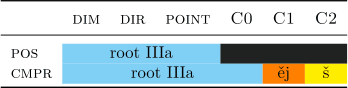
An example of a lexicalisation table is given in (29) below for Class I.

• (29) Class I

  

The column headings represent the features in the functional hierarchy that we have argued for in the previous section, and the different rows represent the forms of the positive and the comparative of Class I adjectives, respectively. A form that spans different columns is a portmanteau morpheme, i.e. one that lexicalises more than one feature. The black shading below C0-C2 indicates that these projections are absent in the positive degree.

Our account of Class I is based on the idea that roots in this class only lexicalise dim and dir. Since such roots fail to lexicalise all the features of the positive, they need the stem marker to lexicalise the point projection. This is shown on the first line of the lexicalisation table (29).

The analysis of the comparative is depicted on the bottom row in (29). It assumes that the stem marker can lexicalise not only point, but also the lowest comparative projection C0. The markers ěj and š then lexicalise C1 and C2 respectively.

The lexical items needed for this analysis are provided in (30).

• (30)

  

In order for the analysis to work smoothly, we need to make explicit an assumption, which is that a lexical item may lexicalise all the features it is specified for, or a subset of them. We need this to allow the stem marker to lexicalise just the point feature in the top row in (29). Since point is contained in the entry (30b), may be used to lexicalise just this feature.

We will refer to this as the Superset effect, and we will take it for granted in the following discussion. In the theory of Nanosyntax, this effect follows from the matching condition, which defines when an entry matches the structure, and it is sometimes referred to as The Superset Principle (Starke, 2009). We come to the exact wording of the matching condition in Sect. 7.

Let us now turn to Class II. Our analysis of this class assumes that, since the roots of this class have no overt stem marker in the positive, they can lexicalise all the features of the positive, as shown in (31). All the other lexical items keep their specification as in (30).

• (31) /Class II root/ ⇔ [dir dim point]

With this lexical entry, the root is able to lexicalise all the features of the positive without the need for any extra stem marker (see the top row in (32)).

• (32) Class II

  

In the comparative, the feature C0 cannot be lexicalised by the root, since the root does not contain this feature. Therefore, the stem marker - appears as the lexicalisation of this feature. Since is also specified for point, recall (30b), it also lexicalises this feature. The comparative markers ěj and š lexicalise C1 and C2, respectively, which is what they also do in Class I.¹²

Let us now turn to the Class IIIa. This class can be accounted for under the assumption that its roots lexicalise all the features from dim up to and including C0, as in (33).

• (33) /Class IIIa root/ ⇔ [dir dim point C0]

With this specification, the root can lexicalise all the features in the positive, as on the first row of (34). Recall that due to the Superset effect, the root need not lexicalise all the features it is specified for, which makes it a good match in the positive degree, despite the absence of C0 in the structure of the positive.

• (34) Class IIIa

  

In the comparative, the roots of Class IIIa lexicalise all the features up to C0, explaining the absence of , as well as the presence of ěj-š, as depicted on the bottom row in (34).

Finally, roots of Class IIIb can be accounted for under the assumption that they lexicalise all the features from dim to C1, see (35).

• (35) /Class IIIb root/ ⇔ [dir dim point C0 C1]

In the positive, the root will (again) lexicalise all the features (not using its C0 and C1 specification due to the Superset effect). We depict this on the top row in (36).

• (36) Class IIIb

  

In the comparative, the root lexicalises all the features up to C1, leaving space only for š.

Summarising, we have now provided a rather simple account for Classes I-IIIb, without the need to use any context-sensitive rules. Most notably, we have provided an explanation for why in Class II, the marker is only needed in the comparative. Recall that this was unclear previously, where this class required a zero marker that blocked (a default lexicalisation of little a) in the positive. This was a problematic entry, because of the accidental homophony and the negative specification of the context (in the absence of cmpr). None of these problems arises in the current approach, which dispenses with zero markers and replaces their effects by portmanteau lexicalisation.

Our analysis also explains the fact that the alternation between the two allomorphs of the comparative marker (ěj-š vs. š) only arises if the comparative morphemes are directly adjacent to the root, and not if intervenes. This is because the size of is fixed (it cannot go higher than C0), so that it can only trigger one allomorph. Roots, in contrast, can have varying sizes, and as a result of that they can give rise to allomorph alternation. In the following section, we turn to Class IV.

7 The proposal for class IV

This section deals with some interesting analytical challenges offered by the Class IV roots. Let us first remind ourselves of the facts, repeated for convenience in Table 16.

Table 16 Six classes of adjectives

The table shows how, from Class I to Class IIIb, root size increases monotonically, as shown by the increasing number of ‘zero’ morphemes. Furthermore, the size of the root correlates inversely with the number of overt morphemes that follow the root. Class IV does not fit into this picture, in that the presence of in the positive suggests a small root (like those of Class I), but then the absence of in the comparative is puzzling. Looking at the problem from a more general perspective, Class IV reveals a tension between morphological and structural containment. Recall from Sect. 5 that we have adopted here a version of the proposal by Bobaljik (2012), according to which the comparative degree structurally contains the positive degree. In terms of morphology, however, the Class IV comparative is not built on top of the positive: the positive base is truncated, since the stem marker has to be deleted before the comparative marking is added.

This type of marking is quite rare, contradicting a candidate universal proposed by Grano and Davis (2018, 133).

• (37) Candidate Universal Universally, the comparative form of a gradable adjective is derived from or identical to its positive form.

This universal is violated by the type of marking observed in Class IV, since the comparative here is neither derived from nor identical to the positive degree.

In technical terms, the challenge stems from the fact that when we look at the comparative of Class IV, we see that it lacks and has only ěj-š (Class IVa) or just š (Class IVb). This suggests that such roots must be specified for all the features up to C0 or C1 respectively, as on the comparative rows in (38) and (39).

• (38) Class IVa

  

• (39) Class IVb

  

Given the capacity of the roots to lexicalise all the features from dim all the way up to C0 or C1 in the comparative (including the stretch dim-dir-point), the question arises why these adjectives need in the positive (as the realisation of point). The first row of the relevant tables (38) and (39) presents lexicalisations with the included, but this is exactly the puzzling thing: in the comparative, the exact same features (dim-dir-point) are lexicalised by the root, so why is this not an option in the positive? Why does have to appear here?

The question is relevant also in the light of the fact that in Class III, we argued that the ability of the root to lexicalise all the features up to C0 automatically entailed that these roots can also lexicalise all the features of the positive (via the Superset Effect). This was shown in the lexicalisation Table (34) above, repeated for convenience in (40).

• (40) Class IIIa

  

What the Class III roots display is a property that we can informally refer to as shrinkability: a bigger root (size C0P or C1P) can shrink to lexicalise a smaller syntactic structure that is contained in it (pointP). This shrinkability of roots is, in fact, a case of the Superset effect. Put in those terms, the puzzle presented by the Class IV roots is why they cannot shrink to size pointP, given that the Class III roots can do exactly that.

However, it turns out that it is possible to resolve this tension in a way that maintains the assumption that the positive is structurally contained in the comparative. We shall do so by adapting a proposal by Blix (2022), who addresses a similar challenge in the domain of number marking. To see how Blix’ idea works, we must consider additional details of the lexicalisation procedure. Once the details are clarified, it turns out that the lexicalisations as given in (38) and (39) are in fact possible, while still preserving the idea that the comparative is built on the positive.

The main feature of the solution stems from the fact that in Nanosyntax, lexical items do not link phonology to a random collection of features. Rather, they link phonology to well-formed syntactic representations (Starke, 2014). Given this idea, (41a-d) provide the updated lexical items of the roots belonging to Classes I-IIIb. The entries still contain the same features as before, but since lexical entries link syntactic representations to phonological representations, the features are structured. And it is precisely this aspect of their format that is going to provide a solution to the conundrum presented by Class IV roots. (The meaning of the circled nodes will be clarified shortly.)

• (41)

  

With the updated format of lexical items in place, let us now also present the Matching Condition on lexicalisation (Starke, 2009), which is often referred to also as the Superset Principle.

• (42) Matching Condition A lexically stored tree matches a syntactic node iff the lexically stored tree contains the syntactic node.

The Matching Condition makes it clear that lexicalisation does not only care about the number of features, but it imposes a stronger requirement, namely constituent identity: a lexical entry only matches a syntactic tree iff it contains an identical tree. Therefore, lexical items can lexicalise the three features of the positive (dim-dir-point) only if these features form a constituent inside the lexical entry.

It turns out that roots of classes II, IIIa and IIIb do contain the constituent corresponding to the positive degree, as highlighted by the circles in (41). The fact that a tree identical to the syntactic tree of the positive is literally contained in the lexical trees of (41) is what allows these roots to lexicalise the structure of the positive without any additional morphology. For convenience, (43) presents the structure of the positive as originally presented in (25a).

• (43)

  

With this background in place, consider the lexical entries that we are proposing for Class IVa and IVb in (44a,b) respectively (taking inspiration from the proposal put forth in Blix, 2022):

• (44)

  

While the constituency of the lexical entries in (44) may appear unusual, they still adhere to the general idea that lexical items are nothing but links between well-formed syntactic representations and phonology. In this approach, such lexical items are in fact to be expected: it is a logical possibility that a particular constituent moves in the syntax (e.g., the constituent [dir dim]), and once it lands higher up in the structure, such a structure (containing a moved constituent in a higher position) is linked to phonology. And this is precisely what the lexical entries in (44) are: they link phonology to a structure in which the dirP has moved from within pointP to the left.

For us, the most relevant point about these lexical items is that they do contain a constituent that has all the features from dim up to C0 or C1: this is the top node of the entries. This constituent is relevant for the lexicalisation of the comparative, where all the relevant features are lexicalised by the root. However, there is no constituent inside the entries that contain the three features of the positive. To make this clear, the features of the positive are highlighted, and it is obvious that they do not form a constituent (let alone one identical to (43)). As a result, these entries cannot lexicalise the positive: they do not contain a constituent identical to it.

To understand how the positive is lexicalised, it is relevant to note that the features dim and dir still form a constituent in both (44a,b), in the form of the complex left branch. Therefore, the roots can still lexicalise these two features. This is because the derivation of the positive proceeds bottom-up, first merging dim and dir. This will create a syntactic constituent that is identical to a constituent contained in (44), so that the root may lexicalise this syntactic constituent. This is exactly what happens in the positive, as depicted in the lexicalisation tables in (38) and (39), repeated below for convenience. However, the feature point cannot be lexicalised along with these two features, and that is why appears in the positive (in a manner that we shall make precise in the next section).

• (45) Class IVa

  

• (46) Class IVb

  

In the next section, we introduce the lexicalisation system of Nanosyntax in detail, and show how the lexical items of roots interact with the syntactic derivation so that the observed patterns are derived. In particular, we shall show how the syntactic derivation will generate constituents that are identical to those in (44), allowing the roots of Class IV to lexicalise all the features up to C0P (Class IVa) or C1P (ClassIVb), as shown in (45) and (46).

8 The derivations

This section provides the basic principles of lexicalisation in Nanosyntax, and shows how they derive the lexicalisation tables of Classes I-IV, as described above in Sects. 6 and 7. This is thus the last step in demonstrating that context-sensitive rules and portmanteau-based lexicalisation are not equivalent systems, and that portmanteau-based lexicalisation allows one to model the facts without the need to introduce multiple cases of accidental homophony or negative conditions on insertion.

Like much of the work in standard minimalism, Nanosyntax (Starke, 2018) assumes that syntactic structures are built step by step by successive application of Merge. In addition, Nanosyntax adopts the idea of cyclic lexicalisation. This means that whenever a new feature is merged, the structure is sent to the interface, where it is determined whether the structure can be lexicalised or not. A structure can be lexicalised if it finds a matching item in the lexicon, where matching lexical items are selected based on constituent identity (recall the Matching Condition in (42)).¹³

When the structure is sent to interface and a matching lexical item is found, the derivation may continue by adding additional features. However, when no matching item is found, the structure is rejected at the interface and sent back to syntax for adjustments. These adjustments correspond to various types of evacuation movements, whose type and order is defined by the so-called lexicalisation algorithm.

• (47)

  

The clause (47a) of the algorithm implements the idea of cyclic lexicalisation: always when a feature is merged, a matching item must be found for the newly created FP. (47b-d) specify various repair options, namely Spec movement, complement movement and backtracking. We will introduce these derivational options as we go.

These operations apply algorithmically, i.e. in the order specified, and blindly, i.e., without any knowledge of whether they succeed or not. The success of each operation is always evaluated against the lexicon, which is why each operation is followed by ‘lexicalise FP’.

Finally, let us mention that the evacuation movements are triggered by the need to lexicalise the structure, and not by the need to check features. This means that they are different from standard feature-driven movements. In Nanosyntax, they are not only different in what triggers them, but also in their implementation. For instance, it is assumed that they do not leave a trace, since they do not give rise to two interpretative positions (unlike feature-driven movements). Therefore, whenever a phrase will be moved due to evacuation movements, the base position will be simply left empty.

With the background in place, let us now turn to the step-by-step derivation of the individual six classes that we have distinguished above. Each class is discussed in a separate subsection.

8.1 Class I

The Class I roots require both in the positive and in the comparative. In the comparative, is followed by ěj-š. The pattern is depicted in the lexicalisation table in (48).

• (48) Class I

  

In (49), we give the lexical items relevant for this class.

• (49)

  

In (50), we present the full stepwise derivation of the positive degree. The derivation starts by merging dim and dir together, producing dirP (50a). After the features have been merged, the resulting phrase must be lexicalised. The DirP in (50a) can be lexicalised by the root, because the entry (49a) is identical to (50a). Successful lexicalisation is depicted in (50b) by circling the dirP. After successful lexicalisation, Merge F continues by adding another feature, namely point, producing (50c).

• (50)

  

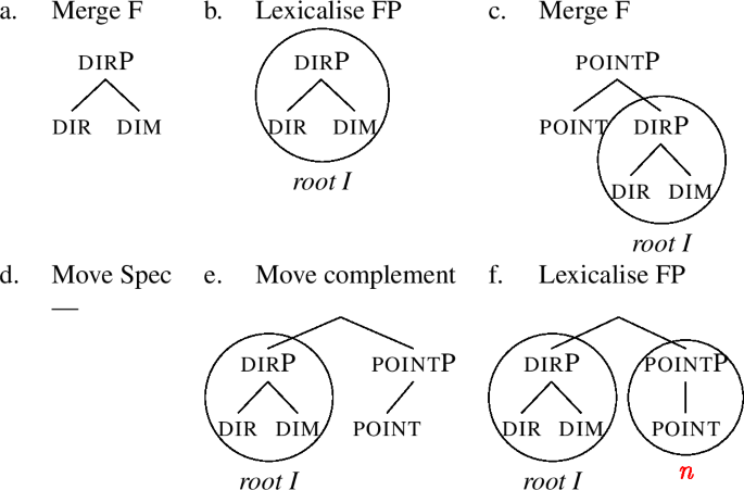
After point is merged, pointP must be lexicalised. However, the root in (49a) does not contain a constituent identical to (50c), therefore, lexicalisation fails. This means that evacuation movements are triggered following the lexicalisation algorithm (47). The first evacuation movement is the movement of the Spec of the complement of the newly added feature. However, the complement in this case has no Spec, so this step does not lead to any change, and lexicalisation fails again (50d). The next step is complement movement. We start from (50c) and evacuate the complement of point out of pointP. The structure we get is in (50e), where the base position of the extracted phrase is simply left empty, in line with our assumption that evacuation movements do not leave traces. Since a pointP with a single daughter is contained in the lexical item for (49b), lexicalisation succeeds, yielding (50f), which represents the correct lexicalisation of the positive degree of the Class I roots.

If we want to derive the comparative form, the derivation must add additional features, starting with C0. The merger of C0 is shown in (51a).

• (51)

  

The structure (51a) does not find a direct match in the lexicon, and so evacuation movements have to apply. Moving the Spec of the complement yields the structure (51b). As we can see in (51c), the remnant C0P finds a match in the lexicon, so C0 is lexicalised along with point by , still in perfect compliance with the lexicalisation Table (48).

The derivation now continues by merging C1 (52a). As there is no match for C1P in the lexicon, Spec movement is tried, yielding (52b).

• (52)

  

However, there is still no match for C1P, so the derivation goes back to (52a), and moves the whole complement, yielding (53a). In this structure, lexicalisation of the remnant C1P succeeds, and the whole structure is lexicalised as root--ěj, still in accordance with the lexicalisation Table (48).

• (53)

  

The derivation continues by merging the final feature of the comparative, C2, yielding (54a). This structure cannot be lexicalised, since there is no match for the C2P in (54a). Therefore, Spec movement is tried, yielding (54b).

• (54)

  

However, even in (54b), there is no match for C2P, containing now only two features, C2 and C1. Therefore, the derivation goes back to (54a) and moves the whole complement of C2, yielding (55a). In this structure, the remanant C2P contains only a single daughter, the feature C2. This C2P can be lexicalised by the lexical item š (55b). As a result, we have derived the correct comparative of Class I, namely the root followed by -ěj-š, exactly in line with the lexicalisation Table (48).

• (55)

  

Concluding, this section has shown how the lexicalisation table in Class I arises from the interaction of the proposed lexical entries and the standard Nanosyntactic lexicalisation algorithm (47).

8.2 Class II

The Class II roots do not require any extra morpheme in the positive, while in the comparative, they required the stem marker , followed by ěj-š. The lexicalisation table is depicted in (56).

• (56) Class II

  

It will become relevant in the course of the discussion that the lexicalisation of the comparative in Class II is the exact same lexicalisation as in the comparative of Class I, compare the bottom row of Table (56) with the Class I table in (57), repeated from (48).

• (57) Class I

  

In (58), we give the lexical items relevant for Class II.

• (58)

  

The derivation of the positive degree is quite simple. We merge dim and dir (59a), producing a phrase that can be directly lexicalised by the root (59b).

• (59)

  

When point is added, as in (60a), a direct lexicalisation is possible again (60b). This final tree represents the correct structure for the positive degree in this class, featuring the root and only the root.

• (60)

  

A slightly more complex derivation arises for the comparative. First, C0 is merged on top of the structure of the positive, yielding (61a). This structure cannot be lexicalised by the root, and evacuation movements are therefore triggered. Since the complement has no Spec, this rescue operation fails. When complement movement is tried, we get the structure in (61b). Here we have a C0P with a single daughter, namely C0. Amongst our entries in (58), C0 is only contained in the entry for in (59c). However, the entry does not contain a constituent identical to the C0P as it is found in (61b), as the C0P of (59c) itself contains a pointP, which the C0P of (61b) lacks. As a result, we must conclude that lexicalisation fails in (61b). This is the reason why in the lexicalisation Table (56), the middle row (where lexicalises just C0) is not a viable option.

• (61)

  

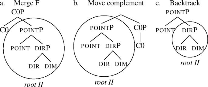
Now, in the lexicalisation algorithm (47), complement movement is the last type of evacuation movement. When this movement fails, there are no more movements to be tried. As a last resort, the so-called backtracking step of the algorithm is activated. The idea behind backtracking is this: in our attempts to derive the comparative, we have added the feature C0 on top of a particular structure, and we could not lexicalise it no matter what we tried. Backtracking makes the derivation go back to the previous cycle and lexicalise it differently, changing the original structure. The C0 is added again, but since it is added to a different structure, lexicalisation of C0 has a chance to succeed.

The backtracking step therefore tells us to return to the previous cycle (i.e., back to when point was added) and try a different option for that cycle. The stage of the derivation when we added point is shown in (60a). Originally, i.e., in (60b), we used lexicalisation without movement. However, since that ultimately failed when we added C0, the algorithm tells us to try some other option. The next option of the algorithm is to move the Spec of the complement, but this option is undefined (62a). Therefore, we go back to (61c) and perform complement movement, yielding (62b). In this structure pointP can be lexicalised as (62c).

• (62)

  

Notice that, as we are trying to produce the comparative, the derivation led us back to the positive, and made us reconsider our previous lexicalisation of pointP: in the positive, it was lexicalised just with the root. Now, due to backtracking, pointP is lexicalised by the root and , exactly as on the bottom row of Table (56).

Another point to note is that now pointP is lexicalised in exactly the same way as with Class I roots, whose derivation was given in (50). Therefore, should we now attempt the derivation of the comparative starting from (62c), we would follow exactly the same steps as in Class I, starting from (51) and proceeding all the way to (55). Therefore, the lexicalisation of the comparative in Class II is exactly the same as the lexicalisation of the comparative in Class I (i.e., root-n-ěj-š). This is the correct result, as already pointed out at the start of this section.

Concluding, this section has shown how the lexicalisation table in Class II arises from the interaction of the proposed lexical entries and the standard lexicalisation algorithm.

8.3 Class III

The Class III roots are characterised by the fact that they have no , neither in the positive, nor in the comparative, where the root is directly followed by ěj-š (Class IIIa) or by š. The lexicalisation tables are depicted in (63) and (64).

• (63) Class IIIa

  

• (64) Class IIIb

  

The entries for the roots are provided in (65); we do not repeat the functional morphemes (, ěj, š) as they remain the same throughout.

• (65)

  

The start of the derivation is the same for both classes of roots. In the derivation of the positive, we only merge features and directly lexicalise, ultimately deriving the positive form in (66d), which is correctly derived as lexicalised by the root only.

• (66)

  

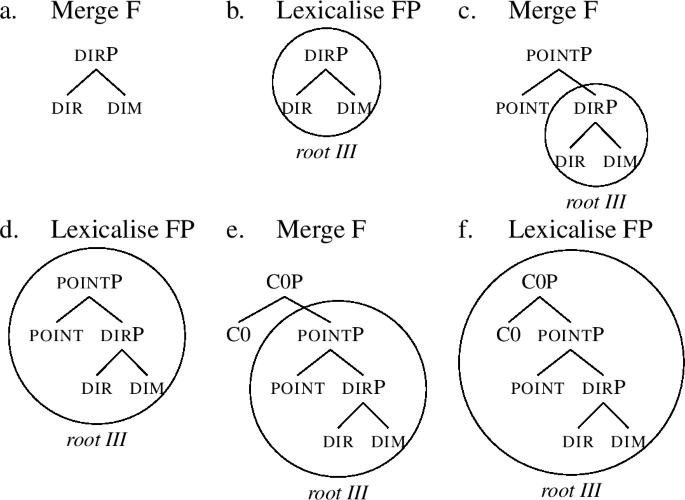
Deriving the comparative also starts the same for both subclasses of roots: when C0 is added, as in (66e), both types of roots can lexicalise this constituent without any need for movement (66f).

From there, the derivation diverges. When C1 is introduced in the derivation, as in (67a), only Class IIIb roots can lexicalise this constituent directly (67b).

• (67)

  

This line of derivation then derives comparatives with just š: when C2 is introduced on top of (67b), as in (68a), direct lexicalisation fails. Since the complement has no Spec, we show directly the result of complement movement in (68b), where the complement of C2 (i.e., C1P) evacuates out of C2P. The remnant C2P can then be lexicalised by š (68b).

• (68)

  

The derivation of the Class IIIa roots is different. With these roots, when C1 is introduced, as in (69a), lexicalisation fails. Therefore, evacuation movements are tried. Since the complement of F2 has no Spec, we show directly the result of complement movement in (69b), along with the successful lexicalisation.

• (69)

  

The derivation then continues by merging C2 (70a). Since direct lexicalisation fails, evacuation movements are tried. Spec movement yields a structure that cannot be lexicalised (not shown), so that complement movement is applied. The structure ensuing from this step of movement is shown in (70b), along with the successful lexicalisation.

• (70)

  

In sum, this section has shown how the lexicalisation tables in Classes IIIa and IIIb arise from the interaction of the proposed lexical entries and the standard lexicalisation algorithm.

8.4 Class IV

The Class IV roots have the stem marker in the positive, but lose it in the comparative, where the root is directly followed by ěj-š (Class IVa) or by š (Class IVb). The lexicalisation tables are given in (71) and (72).

• (71) Class IVa

  

• (72) Class IVb

  

In (44) above, we have already proposed the lexical entries needed to derive the behaviour of this class. We repeat them in (73) for convenience.

• (73)

  

In the remainder of this section, we describe the derivations step by step. The start of the derivation is the same as in all the classes we have discussed so far, with the merger of dir and dim (73a). At this point, both types of Class IV roots can lexicalise this constituent (73b).

• (74)

  

When point is merged (74c), neither of the lexical entries in (73) contains the relevant constituent, which is why evacuation movements are tried. Spec movement leads to no result, since the complement of point in (74c) has no Spec. Complement movement is therefore tried next, yielding (74e). The remnant pointP is lexicalised by (74f), and this is the correct form of the positive.

The derivation of the comparative proceeds as follows. First, C0 is merged to (74f), yielding (75a). Since there is no match, Spec movement takes place (75b). As in Class I, the remnant C0P can be lexicalised by (75c).

• (75)

  

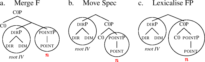
Note at this point that for roots of Class IVa, the structure (75c) is identical to the lexical item corresponding to the root, recall (73a). Thus, for Class IVa roots, the structure (75c) is realised by the root alone, as in (76).

• (76)

  

The derivation continues from (76) by merging C1 on top of it, yielding (77a). Since lexicalisation fails, Spec moves, producing (77b).

• (77)

  

There is no lexical item matching C1P, the derivation therefore goes back to (77a) and moves the complement. We obtain (78a), where the remnant C1P can be lexicalised by ěj, see (78b).

• (78)

  

The derivation continues by merging the final feature of the comparative, namely C2, yielding (79a). This structure cannot be lexicalised (there is no match for the C2P in (79a)). Therefore, Spec movement is tried, yielding (79b). However, even in (79b), there is no match for C2P, containing now only two features, C2 and C1.

• (79)

  

Therefore, the derivation goes back to (79a) and moves the whole complement of C2, yielding (80a). In this structure, the remnant C2P contains only a single daughter, the feature C2. This C2P can be lexicalised by the lexical item inserting š (80b).

• (80)

  

The derivations for the positive and the comparative correspond exactly to what we have in the lexicalisation Table (71) above, repeated in (81) below, but with a minor change. To mark the fact that the IVa roots cannot shrink to pointP size, we have added an asterisk in the point column. Even though the roots are of size C0P, they cannot shrink to pointP because of the shape of their lexical entry. Observe that these roots can shrink to size dirP or smaller, since constituents of this size are contained in their lexical entry.

• (81) Class IVa

  

The only thing that remains is to finish the derivation of Class IVb. In order to do so, we go back to the stage of the derivation where Classes IVa and IVb diverge, namely at the point where C1 is merged. In the case of the Class IVa roots, this required (unsuccessful) spec movement, followed by complement movement, and lexicalisation of the remnant C1P as ěj. In the case of the Class IVb roots, however, starting from (82a), Spec movement is going to be successful, since it creates a structure that exactly matches the lexical specification of the Class IVb roots (73b). As a result, the whole tree in (82b) is lexicalised by the root.

• (82)

  

When C2 is subsequently added (83a), lexicalisation without movement fails. Evacuation movements therefore apply, first Spec movement (not shown, since it fails) and ultimately complement movement, which yields (83b). This structure corresponds to the correct comparative structure of Class IVb, where the root in the comparative is followed by š only.

• (83)

  

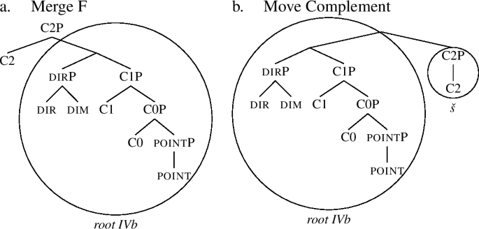
For completeness, we repeat the lexicalisation table for this class, again with asterisks added to those cells that represent sizes to which the lexical tree cannot shrink.

• (84) Class IVb

  

At this point, we have completed the demonstration of the claim that a portmanteau-based approach to allomorphy is capable of encoding the distribution of the stem markers in Czech without the need to introduce any accidental homophony, disjunctive specifications, or negative conditions on insertion.

As a final point in this section, we want to reflect on the general properties of the analysis of Class IV. Recall that this is a special class where the comparative is not based on the positive, violating a proposed candidate universal by Grano and Davis (2018). As has become clear, a crucial aspect of our account is that the lexical entries are not defined purely in terms of how many features they contain, but also how these features are structured. For instance, Class IIIa roots have the same features as Class IVa roots, but they differ in whether they can lexicalise the positive on their own. The difference is in the structure of the features, not in their number.

This presupposes that lexical entries must contain structured constituents, rather than unstructured collections of features, a possibility entertained in Vanden Wyngaerd (2018), as well as in the spanning literature (e.g. Ramchand, 2008; Svenonius, 2012, 2016; Merchant, 2015). However, our results indicate that to deliver all the necessary contrasts (especially between Classes III and IV), structured lexical entries are required.

9 Conclusion

The goal of this paper was to compare two approaches to allomorphy: one based on context-sensitive rules, and the other based on portmanteau lexicalisation. Our general point is that the theories are not equivalent and that the types of allomorph distributions that can be described by the two systems diverge. In particular, we argued that in order to capture the distribution of the stem marker in Czech adjectives, an account based on context-sensitive rules requires postulating multiple homophonous markers and invokes negative conditions on their context. In contrast, the portmanteau-based approach handles these facts without any of these unwanted stipulations. We further provided a detailed demonstration of how this is achieved in the portmanteau-based approach using a standard version of Nanosyntax (Starke, 2018).

Along the way, we noted that some of these patterns are interesting in and of themselves, in particular Class IV, which violates a candidate universal proposed in Grano and Davis (2018). The candidate universal says that the comparative degree should always be based on the form of the positive, which is not the case in Class IV, as the stem marker disappears in the comparative. The system we have proposed allows this pattern to be captured without giving up on the idea, argued convincingly for in Bobaljik (2012), that the structure of the positive is contained in the comparative.

References

Banerjee, N. (2021a). On the interaction of portmanteaux and ellipsis. Ph. D. thesis, MIT, Boston.
Banerjee, N. (2021b). Two ways to form a portmanteau: Evidence from ellipsis. In P. Farell (Ed.), Proceedings of the Linguistic Society of America (Vol. 6, pp. 39–52).
Baunaz, L., & Lander, E. (2018). Nanosyntax: The basics. In L. Baunaz, K. De Clercq, L. Haegeman, & E. Lander (Eds.), Exploring nanosyntax (pp. 3–56). Oxford: Oxford University Press.
Blix, H. (2022). Interface legibility and nominal classification: A nanosyntactic account of Kipsigis singulatives. Glossa, 7(1), 1–46.
Bobaljik, J. (2012). Universals in comparative morphology. Cambridge: MIT Press.
Caha, P. (2017). Suppletion and morpheme order: Are words special? Journal of Linguistics, 53(4), 865–896.
Caha, P. (to appear). Nanosyntax: Some key features. In A. Alexiadou, R. Kramer, A. Marantz, & I. Oltra-Massuet (Eds.), The Cambridge handbook of distributed morphology. Cambridge: Cambridge University Press.
Caha, P., De Clercq, K., & Vanden Wyngaerd, G. (2019). The fine structure of the comparative. Studia Linguistica, 73(3), 470–521. https://doi.org/10.1111/stul.12107.
Choi, J., & Harley, H. (2019). Locality domains and morphological rules. Phases, heads, node-sprouting and suppletion in Korean honorification. Natural Language and Linguistic Theory, 37, 1319–1365.
Christopoulos, C., & Zompí, S. (2023). Taking the nominative (back) out of the accusative. Natural Language and Linguistic Theory, 41, 879–909.
Chung, I. (2007). Suppletive negation in Korean and distributed morphology. Lingua, 117, 95–148.
Cortiula, M. (2023). The Nanosyntax of Friulian Verbs. An Analysis of the Present and Past in Tualis Friulian. Ph. D. thesis, Masaryk University, Brno.
De Clercq, K., Caha, P., Starke, M., & Vanden Wyngaerd, G. (to appear). Nanosyntax: State of the art and recent developments. In P. Caha, K. De Clercq, & G. Vanden Wyngaerd (Eds.), Nanosyntax and the lexicalisation algorithm. Oxford: Oxford University Press.
De Clercq, K., & Vanden Wyngaerd, G. (2017). *ABA revisited: Evidence from Czech and Latin degree morphology. Glossa, 2(1), 1–32. 69.
De Clercq, K., & Vanden Wyngaerd, G. (2019). Negation and the functional sequence. Natural Language and Linguistic Theory, 37(2), 425–460.
Embick, D., & Marantz, A. (2008). Architecture and blocking. Linguistic Inquiry, 39(1), 1–53.
Grano, T., & Davis, S. (2018). Universal markedness in gradable adjectives revisited. The morpho-semantics of the positive form in Arabic. Natural Language and Linguistic Theory, 36(1), 131–147.
Halle, M., & Marantz, A. (1993). Distributed morphology and the pieces of inflection. In K. Hale & J. Keyser (Eds.), The view from building 20 (pp. 111–176). Cambridge: MIT Press.
Janků, L. (2022). The Nanosyntax of Czech Nominal Declension. Ph. D. thesis, Masaryk University, Brno.
Kennedy, C. (1999). Projecting the adjective: The syntax and semantics of gradability and comparison. New York: Garland.
Kennedy, C., & Levin, B. (2008). Measure of change: The adjectival core of degree achievements. In L. McNally & C. Kennedy (Eds.), Adjectives and adverbs: Syntax, semantics, and discourse (pp. 156–182). Oxford: Oxford University Press.
Kennedy, C., & McNally, L. (2005). Scale structure, degree modification, and the semantics of gradable predicates. Language, 81, 345–381.
Křivan, J. (2012). Komparativ v korpusu: Explanace morfematické struktury českého stupňovánína základě frekvence tvarů [Comparative in the corpus: Explanation of the morphematic structure of Czech gradation based on the frequency of forms]. Slovo a Slovesnost, 73, 13–45.
McCawley, J. (1968). Lexical insertion in a transformational grammar without deep structure. CLS, 4, 71–80.
Merchant, J. (2015). How much context is enough? Two cases of span-conditioned stem allomorphy. Linguistic Inquiry, 46, 273–303.
Moskal, B., & Smith, P. W. (2016). Towards a theory without adjacency: Hyper-contextual VI-rules. Morphology, 26(3), 295–312. https://doi.org/10.1007/s11525-015-9275-y.
Neeleman, A., & Szendroi, K. (2007). Radical pro drop and the morphology of pronouns. Linguistic Inquiry, 38(4), 671–714.
Radkevich, N. (2010). On Location: The structure of case and adpositions. Dissertation, University of Connecticut, Storrs, CT.
Ramchand, G. (2008). Verb meaning and the lexicon. Cambridge: Cambridge University Press.
Siegel, D. (1977). The adjacency constraint and the theory of morphology. Proceedings of NELS, 8, 189–197.
Smith, P. W., Moskal, B., Xu, T., Kang, J., & Bobaljik, J. D. (2019). Case and number suppletion in pronouns. Natural Language and Linguistic Theory, 37, 1029–1101.
Starke, M. (2009). Nanosyntax: A short primer to a new approach to language. Nordlyd (Tromsø), 36, 1–6.
Starke, M. (2014). Cleaning up the lexicon. Linguistic Analysis, 39, 245–256.
Starke, M. (2018). Complex left branches, spellout, and prefixes. In L. Baunaz, K. De Clercq, L. Haegeman, & E. Lander (Eds.), Exploring nanosyntax (pp. 239–249). Oxford: Oxford University Press.
Svenonius, P. (2012). Spanning. ms., CASTL.
Svenonius, P. (2016). Spans and words. In D. Siddiqi & H. Harley (Eds.), Morphological metatheory (pp. 201–222). Amsterdam: John Benjamins.
Vanden Wyngaerd, G. (2018). The feature structure of pronouns: A probe into multidimensional paradigms. In L. Baunaz, K. De Clercq, L. Haegeman, & E. Lander (Eds.), Exploring nanosyntax (pp. 277–304). Oxford: Oxford University Press.
Vanden Wyngaerd, G., Starke, M., De Clercq, K., & Caha, P. (2020). How to be positive. Glossa, 5(1), 1–34.
Wasow, T. (1977). Transformations and the lexicon. In P. Culicover, T. Wasow, & A. Akmajian (Eds.), Formal syntax. New York: Academic Press.
Wiland, B. (2019). The spell-out algorithm and lexicalization patterns. Slavic verbs and complementizers. Berlin: Language Science Press.
Williams, E. (2003). Representation theory. Cambridge: MIT Press.
Author information
Authors and Affiliations
Corresponding author
Ethics declarations
Competing Interests
The authors have no competing interests to declare.
Additional information
Publisher’s Note
Springer Nature remains neutral with regard to jurisdictional claims in published maps and institutional affiliations.
Rights and permissions
Springer Nature or its licensor (e.g. a society or other partner) holds exclusive rights to this article under a publishing agreement with the author(s) or other rightsholder(s); author self-archiving of the accepted manuscript version of this article is solely governed by the terms of such publishing agreement and applicable law.
About this article
Cite this article
Caha, P., De Clercq, K. & Vanden Wyngaerd, G. Allomorphy without context specification: a case study of Czech adjectival stems. Morphology (2024). https://doi.org/10.1007/s11525-024-09430-1
Received:
Accepted:
Published:
DOI: https://doi.org/10.1007/s11525-024-09430-1