Obtaining Laws Through Quantifying Experiments: Justifications of Pre-service Physics Teachers in the Case of Electric Current, Voltage and Resistance

Abstract

The language of physics is mathematics, and physics ideas, laws and models describing phenomena are usually represented in mathematical form. Therefore, an understanding of how to navigate between phenomena and the models representing them in mathematical form is important for a physics teacher so that the teacher can make physics understandable to students. Here, the focus is on the “experimental mathematization,” how laws are established through quantifying experiments. A sequence from qualitative experiments to mathematical formulations through quantifying experiments on electric current, voltage and resistance in pre-service physics teachers’ laboratory reports is examined. The way students reason and justify the mathematical formulation of the measurement results and how they combine the treatment and presentation of empirical data to their justifications is analyzed. The results show that pre-service physics teachers understand the basic idea of how quantifying experiments establish the quantities and laws but are not able to argue it in a justified manner.

1 Introduction

Physics ideas, laws and models describing phenomena are usually represented in mathematical form. Therefore, an understanding of how to navigate between phenomena and the models representing them in mathematical form is important for a physics teacher so that the teacher can make physics understandable to students. This means that a teacher can explain and argue physics knowledge in a rational way and order combining different activities and representations (e.g., experiments and mathematical models) into a coherent whole.

Mathematics is an important part of representing physics knowledge. But there are relatively few cognitively oriented studies about why mathematics’ role in physics is so important (Tweney 2012). One reason could be that it allows model-based reasoning that is similar to how diagrams and gestures are used in the reasoning of physics (Tweney 2012). Physical phenomena can be represented using mathematical expressions, and many expressions can also be represented visually (Tweney 2012). In physics education, mathematics’ role in physics is examined in the contexts of problem solving and modeling (Uhden et al. 2012). Uhden et al. (2012) examine the role of mathematics in physics in two roles: the technical role (algorithmic use of mathematics) and structural role, where mathematics and physics are conceptually entangled. They emphasize the structural role, where physical ideas are conceptually translated into mathematical language, and in this process, the different levels of mathematization are tracked (Uhden et al. 2012).

In this study, the relation of physics and its mathematization is discussed in the context of a pre-service physics teachers’ laboratory course. Thereby, the focus is on the “experimental mathematization,” and how the laws or mathematical definitions describing phenomena are obtained through quantifying experiments. For a teacher, it is important to understand how the laws and definitions are or can be established, because an inherent part of understanding the content knowledge is the processes producing the knowledge. However, this understanding has to serve the needs of a teacher. It is good to know the complexity and creativity behind the historical development of the knowledge being taught, but for teaching the content knowledge, the historical processes have to be simplified. Therefore, we have developed the didactical reconstruction of quantifying experiments to serve the pre-service physics teacher education. Next, the quantifying experiments are introduced, and examples of them are given in cases of electric current, voltage and resistance. Then, laboratory reports of pre-service physics teachers are analyzed, and the way the teachers established the empirical formulae of quantities of electric current, voltage and resistance is discussed. The results show that the pre-service physics teachers understand the experimental mathematization process but are not able to explain it in a coherent way, and gaps between the procedural elements remained.

2 Background: Quantifying Experiments Introduced in Physics Teacher Education

Quantifying experiments transform qualities and qualitative dependencies into quantities and laws (Koponen and Mäntylä 2006; Mäntylä and Koponen 2007). Therefore, this process of quantification could be called “the experimental mathematization.” It resembles Thomson’s “inductive” goal of experiments: the establishment of mathematical laws and the formation of theories (Smith and Wise 1989). However, the application of quantifying experiments is based on the generative view of the experiments’ role in knowledge formation, where experiments and theoretical knowledge are intertwined instead of pure inductive (or deductive) procedures (Koponen and Mäntylä 2006). The quantifying experiments are always based on previous research, and therefore, they create a structured network of quantities and laws (Mäntylä and Koponen 2007), and they give students a scaffolded way of organizing their knowledge of physics, a sort of “empirical concept formation.” It should be noted that the quantifying experiments described here are didactical reconstructions; they have their roots in the actual practices in the history of physics (especially in Faraday’s style of experimenting and in German precision experiments by Helmholtz and Hertz), but are streamlined simplifications for educational purposes (Koponen and Mäntylä 2006; Mäntylä 2013). Often in traditional teaching, the laws and formulas are given, and then, the role of experiments is to verify the facts presented. In this kind of teaching, the origin of laws and formulas is omitted. In a traditional university student laboratory, the focus is often in the precise treatment of the measurement results, and the concept formation aspects are not discussed. In the school laboratory, which uses a constructivist approach, the concept formation aspect plays a part, but seldom is the process from observations to laws in mathematical form explicitly addressed (Trumper 2003). The aim of quantifying experiments is to connect the observations of phenomena to the laws representing them, so that the pre-service physics teacher has an idea what the meaning of the mathematically expressed law is and how it can be established in instruction.

2.1 Qualitative Experiments Leading to the Quantifying Experiment

In designing a quantifying experiment, first it should be known what to measure. In this, there are several starting points, where experiences, observations and existing theoretical knowledge more or less intertwine. For instance, noteworthy observations (observations that precede theory) can be a starting point for more experimentation (Hacking 2008), or theory may guide the observation and recognition of phenomena (Hanson 1958; Steinle 1997). Therefore, there are many degrees of intertwinement of observations and theory in the history of physics and in instruction; this should be kept in mind so that both “ends” of this pair get the attention they deserve.

Because the emphasis here is on the “experimental concept formation,” qualitative experimentation precedes the quantifying experiment. The kind of qualitative experiments discussed here come close to the exploratory experimentation discussed by Steinle (1997). In the history of physics, the exploratory experimentation has occurred when there has not been a reliable theory or conceptual framework available. Therefore, the aim of exploratory experiments has been to obtain empirical regularities and to develop proper concepts and classifications to formulate the regularities (Steinle 1997). In short, the purpose of qualitative experiments is

• 1. to observe the phenomenon of interest [and sometimes to create the phenomenon to be further explored (Hacking 2008)] and

• 2. to “find” the changing and constant properties leading to the qualitative dependency (Mäntylä 2013).

Following an example of different degrees of mathematization by Uhden et al. (2012), the qualitative dependency could be in form of “the more A, the more B.”

2.2 Designing and Implementing the Quantifying Measurement

The qualitative dependency gives the idea of what to measure, and the theory gives guidelines in designing the measurement system. The designing of measurement system may require inventing an apparatus, making essential approximations, reducing perturbing effects and estimating the allowance for the residues (Kuhn 1961). For educational purposes of learning empirical concept formation, the practical problems of designing quantifying experiments are reduced; the course instructor has already designed the quantifying experiments, but pre-service physics teachers still have to set up the experiments, do the measurements and control the perturbations. During measurement, one variable (A) is varied, and the changes in the other variable (B) are measured. For simplifying the measurement process, there is no iteration of measurements (Thomson and Tait 1867). However, it is customary to take a minimum of five different measurements, where A is varied and B is measured in order to observe the dependency between the variables reliably.

2.3 From Measures to Empirical Formula

The next stage is to handle the measurement results. In the case of verifying or conforming experiments, it could be enough to show in different columns of the table the measured values and the calculated values based on theory and find “reasonable agreement” between the values (Kuhn 1961), but now the goal is to examine the qualitative dependency such as “more A, more B” in more quantitative form. In representing the experimental results, the methods discussed by Whewell (1840) and Thomson and Tait (1867) are applied. In Whewell’s “method of curves,” a curve is drawn, where “the observed quantities are the ordinates, the quantity on which the change of these quantities depends being the abscissa” (Whewell 1840, XLIV). The curve, the graphic representation of the results make it possible to detect the regularity or irregularity in the forms of the curve and further to detect the laws, which the measured quantities follow, an “empirical formula” (Whewell 1840, Thomson and Tait 1867). Usually, the drawing of the curve requires interpolation, fitting a curve between the measurement points (Thomson and Tait 1867); also extrapolating the curve to the ordinate is often required in order to find the form of empirical formula. Although the ideas of Whewell, Thomson and Tait were expressed as early as the nineteenth century, they are still recognizable in contemporary physics textbooks. In addition, one reason for the educational success of the microcomputer laboratories is due to the ease of drawing these curves. That allows learners to analyze the relationships between variables and in that way to understand the scientific concepts (Trumper 2003). In the didactical reconstruction of quantifying experiments, the goal of the curve is “straight line.” Then, for example, in the case of “more A, more B” (and the curve goes through origin), there is direct proportionality B ~ A between A and B. This is the next level of empirical mathematization [compare with Uhden et al. (2012, p. 13)]. The slope of the curve represents the constant property observed during qualitative experimentation and follows its magnitude: The quality is transformed into quantity, and the quantitative dependency is the “new” empirical formula (compare with Kurki-Suonio 2011, Fig. 3). Now the empirical formula B ~ A can be written in the more sophisticated level of mathematization: B = C·A (see Uhden et al. (2012, p. 13), where the constant C is the “new” quantity. Then, its defining law becomes C = B/A, which provides the quantity a unit and tells how the quantity’s values can be measured.

Thereby, in the most simple case, the empirical mathematization goes from “more A, more B” to “B ~ A” ending up with “B = C·A.” Of course, the variables are not always directly proportional; for example, “more A, more B” could mean proportionality “B ~ A ².” In that curve, the type of the proportionality is not so obvious, and therefore, on the abscissa, the values of A ² are represented instead of A in order to see the direct linear proportionality. This applies also for the case of “less A, more B,” the inverse proportionality: In the abscissa, the values 1/A are represented and linear proportionality B ~ 1/A can be seen. In all but the simplest cases, finding the right type of proportionality is an intuitive process; there is no simple recipe that can be applied to every case. For example, dimensions give a hint about the proportionality between kinetic energy and velocity: E _k = [Nm] = [kg(m/s)²], which suggests that E _k ~ v ². Snell’s law sin β ~ sin α is an example of a proportionality that can only be found with a help of a prediction provided by a model describing the phenomenon, in this case, the Huygens principle.

2.4 Comparative Quantifying Experiments

Sometimes it is not possible to quantify a quantity based on known quantities. Then, the quantifying experiment is designed so that the properties involved in the phenomenon are compared (Jammer 1961). An example of this is Mach’s way to quantify mass (Jammer 1961). Many of the SI base units can be obtained through the comparative quantifying experiments. These measurements resemble “nomic measurements” discussed by Chang (2001). The problem in these measurements lies in a circularity of such measurements, for example, in case of temperature, “we need a thermometer, which is the very thing we are trying to create, to measure the temperature” (Chang 2001, p. 251). In the didactical reconstruction of these kinds of experiments, a method is developed to vary the quality to be quantified in a controlled way. This is often done by choosing a prime measure (like the inertia of a wheeled cart or electric current of a bulb) and then multiplying it (by attaching similar carts together or connecting similar bulbs in parallel). Fixing the unit of the quantity would be done by defining a standard for the prime measure. For example, one could state the mass of a certain wheeled cart as a standard mass and define its unit. In school experiments, one seldom can define true SI units this way, but the very idea can be introduced.

2.5 Simplifying the Treatment of Data for Concept Formation Purposes

It should be noted that while quantifying experiments include measurements and line fitting, formal uncertainty analysis is very seldom needed. Knowing the uncertainty of an experimental result is important when one tests predictions derived from existing laws or records data for some practical purpose, e.g., statistics. However, the role of quantifying experiments is to create new concepts. Quality of the measurement must be good enough so that the linear dependency indicated by the graph is unquestionable by the naked eye. It must appear clear just by looking that only a straight line can be meaningfully fitted to the data, and the deviation of the data points from the line is insignificant. In many cases, even the value of the slope is irrelevant; what is important is how the slope reacts when the quality under investigation is varied. While performing a quantifying experiment and its data analysis that reveals an empirical formula leading finally to new law, the learner should be free to concentrate on the concept formation, where the empirical mathematization is of importance. Therefore, in the implementation of the quantifying experiments in the pre-service physics teacher education, the procedures of estimating the uncertainty of measurements are omitted. However, the uncertainty of measures is already handled in the traditional physics laboratory course, where the objectives lie closer to the measurement procedures instead of concept formation aspects.

3 Quantifying Experiments Contextualized: Electric Current, Voltage and Ohm’s Law

Next, we immerse quantifying experiments in more detail through cases of electric current, voltage and Ohm’s law. They were chosen because they offer examples of “normal” quantifying experiments (Ohm’s law and resistance) and comparative quantifying experiments (electric current and voltage). Later, the pre-service physics teachers’ laboratory reports on these experiments are analyzed and discussed.

3.1 Electric Current

Electric current is a quantity describing the state of an electric circuit (macroscopic, phenomenological interpretation). Electric current can be observed through its effects in a closed circuit. These observable effects include, for instance, light, heat and magnetic interaction. Magnetic interaction can be observed, when a compass needle turns near a wire of closed current-carrying electric circuit (the famous Ørsted experiment). These effects can be used as indicators of the strength of electric current in different situations. For example, by comparing the brightness of bulbs, it can be inferred that the current divides equally between similar lamps connected in parallel and in a circuit without branches, there is same current everywhere (Kirchhoff’s first law qualitatively). Further, by comparing the brightness of one bulb connected to a battery to the brightness of two similar bulbs connected in parallel, it can be inferred that the electric current through the battery is double in the case of the parallel connection.

In this case, we cannot quantify electric current based on known quantities; instead, we have to find a way of conducting comparative measurement. The parallel connection of similar bulbs gives us a method to vary electric current in a controllable manifold way: one bulb, one “measure” of electric current from the battery; two bulbs in parallel, two “measures” of electric current from the battery, etc. Then, we need a way to measure the strength of electric current through one of its effects. The magnetic force between a bar magnet and a coil carrying the current is chosen as the effect. The magnetic force (F) can be measured with a scale using the setup shown in Fig. 1. Bulbs are permanently connected in parallel, and current through every bulb is the same (I ₀). By different connections of the coil, electric current through the coil (I) is varied and the magnetic force F is measured. The results are represented as a (F, I) graph. A straight line can be fitted through the data points and the origin, which shows direct proportionality I ~ F. Thus, measuring electric current strength can be based on measuring the magnetic effect of the current. This justifies the use of moving coil instruments in current measurements.

Fig. 1

Diagram of the measurement system in the case of quantifying experiment of electric current

3.2 Voltage

Voltage is also a quantity that requires a comparative quantifying experiment. First, voltage is a quantity describing the battery’s (or voltage source’s) property to cause electric current in a closed circuit. We can observe that the more batteries we have in series, the brighter the bulb of the circuit; in parallel connection of batteries, this does not happen, and voltage across the bulb stays the same. Connecting more bulbs in series with a battery, the bulbs become dimmer and dimmer, and the current decreases. When adding a bulb and a battery in series at a time, the brightness of the bulbs remains the same. The bulb also affects the current. This leads to the inference that voltage appears across any two points in a circuit, not only in battery (in cases of other components than voltage sources, this is sometimes called voltage drop). This idea can be represented in the form of a step-and-level model of potential represented in Fig. 2.

Fig. 2

Circuit diagram of the qualitative experiment of voltage and the step-and-level model of potential

In the quantifying experiment, the voltage (U) is multiplied by connecting similar batteries in series: one battery, one “measure” of voltage; two batteries, two “measures” of voltage, etc. A wire is connected with these batteries as is shown in Fig. 3. The wire is used instead of bulbs, and the lower set of batteries drives current through the wire. Because the wire is homogenous, it is assumed that the potential changes uniformly along the wire. Therefore, the measurement of voltage might be based of finding a point of equal voltage on the wire and measuring the length of wire to this point. As is shown in Fig. 3, a galvanometer is used as a “zero instrument”: The connection point A of the galvanometer in comparison battery “row” is changed and then the point B on a wire where the galvanometer shows 0 is sought. The length of the wire (L) to point B is measured. The results are represented in a (L, U) graph, and a line is fitted that shows a direct proportionality U ~ L. Voltage of one battery can now be taken as a reference U ₀. An unknown voltage U _x can be measured using U _x = (L _x/L ₀)U ₀, where L _x and L ₀ are the wire lengths corresponding to U _x and U ₀.

Fig. 3

Diagram of the measurement system in the case of quantifying experiment of voltage

However, measuring voltage with this method is too tedious for further practical work. Therefore, a voltmeter must be introduced, even if its working principle cannot yet be explained. Readings of a voltmeter are compared to voltage values measured by the wire method, and a direct proportionality is observed. Therefore it may be assumed that the voltmeter also measures voltage, and the meter can be used in further experiments.

3.3 Ohm’s Law and Resistance

Resistance (R) can be quantified through electric current and voltage, so this is the “simple” case of quantifying experiments. Resistance describes a component’s ability to resist electric current. This can be a qualitative experiment using wires of different lengths, thicknesses and material and seeing the changes in current. For example, in the case of varying the length of wire, it is inferred that the longer the wire is, the smaller the current is. In the next experiment, the component in the circuit is the same, but the voltage across the component is increased. It is observed that the current also increases: “more U, more I.”

In the quantifying experiment, the voltage U is varied, and the current I is measured. A diagram of the measurement system is represented in Fig. 4. Then, the component in the circuit is changed (e.g., metal wire of different thickness or material), and the measurements are repeated. The measurement results are represented in (I, U) coordinates, and curves are fitted. As a result, we have several straight lines with different slopes, each for a certain wire. This shows a direct proportionality U ~ I, and because of the lines with different slopes, the empirical formula can be written in form U = RI, where R is the quantity describing the component’s ability to resist the current.

Fig. 4

Circuit diagram of the measurement system in case of quantifying experiment of resistance

4 Design of the Study and Research Methods

The interest here is on the sequence from qualitative experiments to mathematical formulations through quantifying experiments in the case of electric current, voltage and resistance in pre-service physics teacher education. More specifically, the aim is to examine how pre-service physics teachers reason and justify the mathematical formulation of the measurement results and how they combine the treatment and presentation of empirical data in their justifications. The answers to the research questions can be seen reflecting the pre-service physics teachers’ understanding of how the empirical formulas or laws can be established, which is an important part of physics teachers’ knowledge. The specific research questions of the study were:

• 1. How do pre-service physics teachers describe in their laboratory reports the establishments of electric current, voltage and resistance?

  • i. How pre-service physics teachers use procedures in their description?

  • ii. How pre-service physics teachers justify the different steps in their description?

• 2. How do pre-service physics teachers explain the formulation of physical laws?

• 3. What do pre-service physics teachers see as important in the laboratory course and what is the role of quantifying experiments in it?

The research questions are answered by analyzing pre-service physics teachers’ laboratory reports and interviews of voluntary pre-service teachers. It should be noted that the reports were done in small groups; therefore, the answer to the first research question represents the consensus of a group of pre-service physics teachers. Before giving details about data and its analysis, an overview of the laboratory course and the specific topic of DC circuits are given.

4.1 General Context and Participants

The study was carried out in course called “Experiments in the School Laboratory II” (5 ECTS) in the Department of Physics, University of Helsinki in the spring semester 2013. The participants were third- or fourth-year pre-service physics teachers (N = 20), of which seven had physics and ten had mathematics as their major subject; one was a chemistry student and two had a background in engineering. All students had studied at least 25 ECTS of physics (introductory courses) and the preceding teacher’s laboratory course. The pre-service physics teachers are trained to teach at the secondary level of school. The twenty students formed six groups of three students and one pair, and they worked in these groups during the course in planning and implementing the experiments and in reporting them.

4.2 The Course: Experiments in the School Laboratory

The goal of the laboratory course is to familiarize pre-service teachers with the empirical concept formation described in Sect. 2. During the course, pre-service teachers learn to think about the experimentation from the teacher’s viewpoint and learn both the possibilities of modern measuring equipment and the use of a simple and affordable apparatus. The verifying use of the experiments has a subsidiary role because the students are already familiar with such experiments.

The duration of one laboratory course is one semester (14 weeks). The course has one 90-min lecture per week and one guided 4-h laboratory session per week for conducting the planned experiments. The laboratory is open, so the pre-service physics teachers can also use the laboratory outside of the guided sessions. During the laboratory courses, students plan and implement five sets of laboratory experiments in small groups covering certain topics; two compulsory topics (Basic concepts of dynamics, DC circuits) and three are freely chosen among 16 different topics (e.g., energy in mechanics, heat and work, sound, modern physics). The topics are covered during lectures so that students see the essential experiments of all topics. In addition, during lectures e.g., the use of microcomputer-based laboratories, video analysis in school experiments and safety issues are discussed. Any experiment can be applied to school physics, although some require equipment seldom available in schools.

The plan includes description of the experiments, equipment and a concept map that shows how the concept formation proceeds based on the planned experiments. The instructor gives feedback from the plan, and then, a student group implements the experiments, and the instructor helps the group when needed. Finally, students write a report, where they describe the experiments, present the measurement data, draw graphs, and finally, conclude the mathematical models or laws depicting features of the phenomena under investigation. A concept map, which shows the experiments’ role in connecting concepts (e.g., phenomena, quantities, laws) is included in the report.

The instructor evaluates, for example, how empirical concept formation is actualized (how the qualitative experiments, quantifying experiments and verifying experiments are used in concept formation), can the experiments be repeated based on the description, coverage of qualitative experiments, results and data handling of quantitative experiments, idealizations and genuine ideas.

4.3 Laboratory Work Topic: Direct Current Circuits

This study covers only a part of the whole set of experiments done within the DC circuit topic; therefore, to give an idea of the whole set, a short overview of the topic is given. The goal of the topic was to plan a connected set of teaching experiments covering DC circuits and which takes into account the secondary students’ premises. The goals and the contents were discussed during one 90-min lecture. The pre-service physics teachers had already studied the first part of the laboratory course, where they had completed two laboratory reports. Therefore, the approach of the course was familiar to them. The student groups worked at their own pace, therefore the completion varied from 2 to 4 weeks. The plan consisted of three parts: experimental concept formation, taking into account the students’ premises, and the concept map showing the “teaching order” and the connections of the experiments. In experimental concept formation part, the following experiments were required:

• Set of qualitative experiments covering electric current phenomenon

• Quantifying experiment of current

• Experiment demonstrating Kirchhoff’s first law

• Set of qualitative experiments covering voltage phenomenon

• Quantifying experiment of voltage

• Experiment justifying the use of voltmeter

• Experiment demonstrating Kirchhoff’s second law

• Set of qualitative experiments exploring resistance

• Quantifying experiment of resistance and Ohm’s law

• Quantifying experiment of resistivity (voluntary)

• Experiment for measuring internal resistance of a battery

• Set of qualitative experiments exploring electric power

• Quantifying experiment of electric power (voluntary)

In the part that took into account the secondary student’s premises, pre-service teachers designed experiments that are built on the known intuitive conceptions of students, e.g., the belief that a battery is a constant source of current or a difficulty to think of the circuit holistically (see e.g., McDermott and Shaffer 1992).

4.4 Data and Analysis

The data consist of seven laboratory reports of student groups and group interviews of the voluntary students (six interviews, 12 students from six different groups). From the laboratory reports, the descriptions of compulsory quantifying experiments (electric current, voltage and resistance) were analyzed, because the interest here lies on the students’ process of obtaining laws through experiments. In a student group, all students took part in conducting the experiments and in writing the report. Therefore, the analysis of reports shows a consensus view of a student group. An excerpt from a student group’s report is given in the appendix. In the analysis, first, the necessary parts or steps of the empirical mathematization, called here procedures, were identified, e.g., Description of measurement or Graph (see Tables 1, 2, 3). In addition, the qualitative experiments, which were crucial for the quantifying experiments, were included in the procedures. For example, the experiment where a current’s magnetic effect is shown is included, because the knowledge of this effect is used in the quantifying experiment by measuring the magnetic force between the coil and magnet by scale. Then, the elements, which connected these different procedures to a logically proceeding “story,” were identified, and they are called here justifications. For example, the observation was made if the crucial qualitative experiments were mentioned in the description of the quantifying experiment or if the empirical formula was based on a graph.

Table 1 Different elements related to the quantification of electric current and their occurrence in laboratory reports

Table 2 Different elements related to the quantification of voltage and their occurrence in laboratory reports

Table 3 Different elements related to the quantification of resistance and their occurrence in laboratory reports

After the course, the voluntary students participated in the group interviews, and there were students from all laboratory work groups except one (Group 4). The duration of interviews was between 30 and 60 min. In the interviews, students were asked about the goals of the laboratory course and the DC circuit topic and what they had learned during the DC circuit topic. The purpose of these questions was to have an idea from the most important ideas that students adopted during the course (research question 3). It was also asked what their ideas were on how physics quantities and laws are or can be formed, and further, if they think that there are several ways of obtaining this knowledge. These questions were intended to be more context independent so that students could answer them from their own perspective, not how they should answer from the laboratory course’s perspective (and aimed at giving an answer to research question 2). Of course, because the students were prepared to answer the questions concerning the laboratory course and DC circuits, it might have affected their views. Nevertheless, the basic purpose was to probe if the students understood the quantifying experiments as didactical reconstructions and that there are also other ways of obtaining the laws. Finally, questions of the procedures of quantifying experiments were asked (e.g., why graphs are drawn or how proportionality between quantities can be detected). In addition, report-specific questions were asked (e.g., is there a reason why you have not extrapolated the curve to the ordinate). The purpose of these questions was to support and deepen the analysis of the laboratory reports. Because there were at least two students at the same time in the interview, there sometimes is only one response to the question if the others did not have anything to add or shared the same opinion. Nevertheless, mostly, the views of individual students came up during interviews. The interviews were transcribed in verbatim and were analyzed through qualitative categorization of students’ responses. The excerpts from laboratory reports and interviews are translations from Finnish. The students in the interview excerpts are coded so that the first number refers to the group number and the last number identifies the group member; for example, student 32 refers to the second student of group 3.

5 Results

Seven laboratory reports of twenty pre-service teachers and six interviews of twelve pre-service-teachers were analyzed. In following the results, the reader is advised, if needed, to return to the descriptions of the quantifying experiments and the crucial qualitative experiments in Sect. 3.

5.1 Pre-service Teachers’ Descriptions of the Establishments of Current, Voltage and Resistance

The procedures, necessary steps of the empirical mathematization, included crucial qualitative experiments, description of measurement (and subsection on what is varied, what is measured), diagram and picture of measurement system, measurement results, graph (with subsection extrapolation) and the result. Because the quantifying experiment uses electric circuit, the diagram is included. From the diagram, it can be difficult to picture the actual measurement system; therefore, the picture of it (photo) is included in the analysis. Here is an example of the procedural element “What is varied, what is measured”:

A metal wire is connected to a voltage source and the voltage across the wire and the electric current through the wire is measured. Electromotive force is varied, and the measurements are conducted with five different voltages. (Resistance, Group 3)

The justifications are the elements that glue the procedures into a logically proceeding argument chain. The important elements of justification were description of the purpose of the measurement, explicit connection to the qualitative experiments, using pictures, graphs and tables in the description (systematic reference to figures and tables), justifying the result (empirical formula) on a basis of the linear proportionality shown in the graph, reflecting the measurement. Here are examples of justification elements from students’ laboratory reports:

When a quantity that describes the strength of electric current is quantified, it has to be proportional to some measurable property of the phenomenon. We chose here the magnetic interaction. (purpose and connection to the qualitative experiment, current, Group 1)

The measurement is repeated with wires of different thicknesses. We perceive that all graphs are straight lines with different slopes. We can infer that U ~ I. The slope of the line describes the metal wire’s ability to resist current, i.e., resistance. This gives us R = U/I. (result is based on graph, resistance, Group 7)

One can see some deviation from the fitted line in the graph. This can be caused by a small differences between batteries (although according to the manufacturer they all were 1.5 V) or from the error in the measurement of length due to the laxity of wire although we tried to tighten it. (reflections of measurement, voltage, Group 2)

5.1.1 Electric Current

In the case of electric current (see Table 1), all groups describe the qualitative experiment showing current’s magnetic effect, but only two groups (1 and 6) mention it in the description of the measurement. Although the parallel connection of bulbs play an important part in producing the manifolds of current in the quantification, only three groups (1, 2 and 4) describe the qualitative experiment of parallel connection. However, no one of these three groups connects the parallel connection to the quantifying experiment. Although almost every group (six groups) presents a picture and a diagram of the measurement system and all present the graph, only three groups (2, 3 and 5) refer to them. All except one group (4) present the result I ~ F, but only three groups justify it using the graph.

5.1.2 Voltage

The crucial qualitative experiments are presented in almost all reports in case of voltage as can be seen in Table 2. This time groups also make a connection to the qualitative experiments in the quantification phase. Group 5 mentions both qualitative experiments, groups 1 and 2 mention only the first qualitative experiment and groups 3, 4 and 6 mention the second qualitative experiment. Groups 2, 3 and 5 continue the systematic references to figures and images. Although the graph and result U ~ L are presented, only two groups (3 and 7) use the graph in justifying the result. Although the measurement was the most difficult from the quantifying experiments, only two groups (1 and 2) reflect the measurement.

5.1.3 Resistance and Ohm’s Law

Table 3 shows the elements in the laboratory reports related to resistance and Ohm’s law. In this case, only three groups (1, 4 and 6) gave a purpose for the quantifying experiment. Only two groups (5 and 6) refer to the qualitative experiments, although every group is presenting them. Presumably students thought that the measurement system is obvious, because two groups (3 and 4) did not present any visualization at all and four groups presented either diagram (groups 2, 5 and 7) or picture (group 1). All groups present a graph and all except one group extrapolate the curves to ordinate. Three groups (3, 6 and 7) present as results both Ohm’s law and resistance, and group 4 does not present a result at all. All groups who present result(s) also justified it/them by graph.

5.1.4 Occurrences of Procedural and Justification Elements in the Laboratory Reports

Almost all groups presented the following procedural elements: qualitative experiments, “what is varied, what is measured,” graph and result. In procedural elements, main deficiencies were found in the qualitative experiment of parallel connection in case of current (43 %), picture of the measurement system of resistance (29 %) and presenting both resistance and Ohm’s law as a result (43 %). The least presented elements were justification elements: systematic references to figures and tables (e.g., 43 % in case of electric current) and reflections (e.g., 29 % in case of voltage) and in cases of electric current and voltage, “the result is based on graph” (43 and 29 %) and in cases of electric current and resistance, the connection to qualitative elements (29 % both). There seems to be a difference between the use of procedure and justification elements, and therefore, the occurrences of elements were calculated together in order to compare the use of these elements and are presented in Table 4.

Table 4 Student groups’ overall occurrence of elements related to the different quantifying experiments (bolded), in addition the procedural elements and justification elements (italicized) are specified

Next, we looked at groups’ use of elements, where occurrence of elements is over 75 % (strong use of elements) or under 50 % (poor use of elements). Moderate use of elements is in between. Group 1 makes a strong use of procedural elements with current (91 %) and justification elements with resistance (80 %), and other use of elements is moderate. Group 2 makes a strong use of procedural elements with all quantities (82, 80, 82 %) and justification elements with current (80 %); however, justification elements with resistance are poorly used (40 %). Group 3 makes a strong use of elements with current (91 %) and justification elements with voltage (80 %). Group 4 makes a strong use of only procedural elements with current (91 %) and a poor use of all justification elements (20 % each). Group 5 makes a strong use of all procedural elements (91, 90, 82 %). Group 6 makes a strong use of procedure and justification elements with resistance (100, 80 %) and a poor use of justification elements with current and voltage (40 % both). Finally, group 7 makes a strong use of procedural elements with voltage and resistance (80, 82 %) and a poor use all justification elements (40, 20, 40 %).

There are altogether 12 cases out of 21 where procedural elements are used strongly and only five cases where justification elements are used strongly. In addition, the average of all occurrences shows the differences of the use of the elements: 80 % average occurrence of procedure and 51 % average occurrence of justification elements (see Table 4, the two last rows of the right column).

If we calculate the average occurrences of procedural and justification elements per group (the two lowest rows of Table 4), three different categories of groups form:

• 1. Strong use of procedural elements, moderate use of justification elements. These groups use the different procedures properly in their reports and justify their uses in a satisfactory way. Therefore, they describe the establishments of laws in a fairly coherent way. Groups 2, 3, 5 and 6 belong to this category.

• 2. Moderate use of procedural elements, moderate use of justification elements. There are deficiencies in the use of procedures; however, the group can justify the uses of procedures in a satisfactory way. This group describes the establishment of laws in a quite coherent but narrow way. Group 1 belongs to this category.

• 3. Strong use of procedural elements, poor use of justification elements. The essential procedures are represented in reports; however, there is a lack of justifications between the procedures. Therefore, the establishments of laws are described in a disconnected way. Groups 4 and 7 belong to this category.

From the interviews, students’ descriptions of the formulations of laws were analyzed. Students from groups 3, 5 and 6 gave satisfactory descriptions. That is in line with the results. From group 4, there were no interviewees.

In an ideal case, student groups would have strong use of both procedural and justification elements. Then, they would have represented the empirical concept formation in a justified manner: The necessary steps from qualitative experiments to the mathematical formula would have been represented, and the steps would have been argued and connected to each other. Altogether, four groups out of seven describe the establishments of laws in a fairly coherent way, and all except one group describe the essential procedures. Clearly, the challenge with pre-service physics teachers lies in how to connect the different procedural elements into a coherent whole.

5.2 Pre-service Physics Teachers’ View of the Formulations of Laws

In the interview, students were asked about how they think that physics quantities and laws are formulated or established. They were also asked if there exist different ways of formulating the laws. Specifying questions were asked if needed. The purpose here is not to give any exhaustive description, rather to see how students think about the formulation of laws from their own perspective. In this, we looked at whether students’ views of the formulation of laws are congruent with the reconstruction of quantifying experiments. We looked also at whether the students understand that there are several justifiable ways of obtaining the physics knowledge such as modeling. The different aspects were recognized and classified from the interview transcription and were formed as the following statements:

• Observations and/or phenomena are the starting points (9/12 students: 11, 12, 21, 31, 32, 51, 52, 61, 62). Most students see that there has to be a concrete starting point, an observation or a phenomenon that requires explanation.

  We observe something new and therefore there is a need to name it (Student 32)

  First, there has to be a phenomenon, then one starts to explore, justify and test it. (Student 51)

• Laws are formulated through experiments (ten students: 11, 12, 31, 32, 33, 51, 61, 62, 71, 72). The direction here is that the experiments precede the laws: The laws are defined through experiments and are represented in mathematical form, which is assigned by the results of the experiment.

  You do experiments and test phenomena with them, what are the dependencies in them. After it, if you find some parameters, variables, which are affecting each other, the mathematics is built up, you get the equation out. (Student 51)

• Laws are formulated by deduction (four students: 31, 33, 62, 72). This is the view where laws are formed first and then they are tested or verified by experiments.

  It has to start from theory, so that you know what you are doing, and then you show by experiments that it is true. (Student 72)

• Laws are formulated through modeling (one student: 32). The student sees that it is also possible to form new knowledge through modeling.

  If the previous theories do not answer all questions, then one can make such theories or models about how things should perhaps be (Student 32)

• Laws can be formulated without the use of experiments, but its validity is uncertain (two students: 61, 62)

  Although you are not able to test the law by experimenting, it still could be valid. Nevertheless, I still feel that it should be observed that it relates to something to a certain extent at least. (Student 62)

• Laws are formulated by manipulating equations (four students: 21, 51, 62, 71). Students see that by deriving equations somehow through different mathematical operations, new knowledge is produced.

  In a lecture, a box is drawn, and then you do some calculations and from somewhere the velocity of light appears. (Student 62)

As can be seen, most students (10/12) think that the laws can be established through experiments. This was expected, because of the context of the study. When it comes to other ways of establishing the laws, there is much more diversity. Four students expressed the familiar deductive view of producing knowledge. Student 32 had a quite sophisticated view of the role of models in knowledge forming. Students of group 6 expressed an idea that laws can be somehow derived from theory, but felt that an experimental verification would improve the validity of such laws. Four students saw that mathematics and using equations somehow leads to new knowledge and an impression that this view is due to the traditional way to teach or lecture physics was transmitted from the interviews. However, altogether nine students out of twelve interviewed students expressed that there is another way of establishing physics knowledge.

5.3 Pre-service Physics Teachers’ View of Their Learning During Laboratory Course and DC Circuit Topic

From the interview questions about the course and DC circuit topic goals and students’ learning it was asked what the most important ideas or aspects were that students had adopted during the course. The responses were classified into two main categories: the aspects of one’s own personal learning and the aspects of development of teacher’s thinking and skills. The aspects of students’ own personal learning were:

• Learn physics (eight students: 11, 12, 21, 33, 52, 61, 62, 72).

  I manage to consolidate the concepts of electricity; it was long since I studied electricity. (Student 52)

• Learn experimental concept formation (six students: 11, 31, 32, 33, 51, 72)

  You don’t look at already made formulas, instead you look at what this data tells you about proportionality, how different quantities and things relate to each other. (Student 72)

• Learn to design and do experiments (six students: 11, 12, 52, 61, 62, 72)

  It was really nice to do the different experiments that you can apply in teaching, because I had not seen any demonstrations at school, so it was good that you saw or did at least once demonstrations with good equipment. (Student 52)

• Learn to do quantifying experiments (two students: 32, 33)

  The quantifying experiments were quite new for me. I have rarely come across them; how you can actually quantify quantities. Those qualifying experiments are generally easier and they are easier for you to design yourself. (Student 32)

• Become familiar with equipment (two students: 11, 72)

  I learned the use of meters when doing experiments (Student 72)

The aspects of learning teacher’s thinking and skills were:

• Learn to teach in an organized way (three students: 12, 31, 72)

  It is about how you design a rational whole about a topic, where do you start, how you proceed in it and then, of course, how you implement the experiments in this concept formation. (Student 31)

• Learn to teach physics through experiments (three students: 12, 62, 72)

  It is good for a teacher to have a clearer picture of how you could teach it [DC circuits] to students and how you do it by using experiments. (Student 12)

• Learn to combine the theory and practice in teaching (two students: 21, 61)

  It is clear that the theory and practice should meet, and the experiments should be designed so that they clearly tell students that this work is about this topic and this phenomenon and they are linked in this way and that way. (Students 21)

• Learn to design clear and simple qualitative experiments for teaching (two students: 71, 72)

  Such small experiments that are easy to do are important, because you can show the basic ideas in very clear way. (Student 72)

As can be seen from the results, the pre-service teachers were in a stage, where they were still learning themselves, and the teacher’s perspective was only starting to develop. However, the didactical reconstruction of using experiments in the laboratory course takes into account the needs of prospective teachers: The experiments pre-service teachers designed and conducted were mostly such that they can be applied in school teaching, for instance the qualitative experiments and the quantifying experiment of resistance. In the case of a quantifying experiment of voltage, four pre-service teachers expressed that the experiment was conceptually difficult, but if a pre-service teacher understands what is done in the experiment, then it could be claimed that the pre-service teacher possesses a good conceptual understanding of voltage and potential. There are also practical aspects of learning such as becoming familiar with the equipment and learning to do experiments, which means that some of the challenges that pre-service teachers face are at the very practical level and clearly, the understanding of empirical mathemazation is a higher-level challenge. However, the pre-service teachers also discuss the experiments’ important role in learning at the metacognitive level, such as learning experimental concept formation or teaching in an organized way.

6 Discussion

Often the entanglement of physics and mathematics is treated as self-evident in teaching and discussing physics. According to Tweney (2012), this should not be the case, and instead more cognitively oriented studies are needed. Also in learning physics, one important goal is to understand the relation between the observed phenomena and their mathematical description. In order to reach this goal, the issue should be addressed in physics teacher education, so that future physics teachers are prepared to handle the relationship between the phenomena and mathematical representation of physics knowledge.

Previously Uhden et al. (2012) have discussed different levels of mathematization, which are essential in the process of “translating” conceptually the physical ideas into mathematical language. However, they have approached this process from the viewpoint of problem solving and modeling. Here, it is suggested that these levels of mathematization can also be approached from the viewpoint of quantifying experiments. In this viewpoint, the mathematization is intertwined with experiments. As such it is not a novel idea; the empirical mathematization method has been discussed, for example, by Whewell (1840), and Thomson and Tait (1867) in the nineteenth century. However, here the process from observations to empirical formula is applied to the needs of physics teacher education. The historical steps and laborious uncertainty estimates are streamlined so that the emphasis is on the empirical concept formation.

The analysis shows that the different degrees of mathematization introduced by Uhden et al. (2012) were well represented in the procedural elements of student groups’ reports. There is high occurrence in elements of qualitative experiments (more A, more B, e.g., more U, more I) and graphs, from where the result is “read” (B ~ A, B = C·A, e.g., U ~ I, U = RI). In addition, analysis shows that on overall, the occurrence of procedural elements was high. This means that mostly pre-service physics teachers understand what is involved in the process of establishing quantities and laws through quantifying elements, what are the necessary steps from observations to empirical formula. However, the deficiencies in representing the justification elements in the reports show that although the pre-service physics teachers know what is needed to formulate the law they are not able to justify and reason in a satisfactory way. For example, the excerpt from a student group’s report (“Appendix”) shows that although the group presents the graph, they do not refer to it in their conclusion of “the interaction of magnetic force is linearly proportional to the magnitude of electric current.” The ability to reason and justify knowledge and to connect the essential elements together is a necessary skill for a teacher; otherwise, the teaching consists of a set of loosely connected activities and statements. The inability to justify the procedure of the quantifying experiment might be explained by the fact that the pre-service physics teachers are still learners of physics themselves, as the interviews showed. Perhaps the ability to justify is possible only when they comprehend better the physics involved.

The pre-service physics teachers’ views of the establishment of physics quantities and laws were versatile in the sense that they believed there is not just one way of reaching physics knowledge. This is a good sign, because although the quantifying experiments are applicable in school settings to a certain extent, their main role is to give to prospective teachers a metacognitive tool that can be used for organizing and ordering knowledge and tying the different activities (experimentation and mathematization) together. However, this does not cover all the aspects needed in learning physics, such as modeling, and the pre-service physics teachers are aware of that. In the interviews, the use of experiments and measurements were described fluently, so clearly the pre-service teachers understand the basic idea of empirical mathematization. On the other side, the role of mathematical models and theoretical knowledge in establishing physics knowledge were quite brief and ambiguous. There were views that perhaps reflect pre-service teachers’ experiences from physics lectures: Equations are mathematically manipulated and then new knowledge appears. The poor descriptions of alternative ways of establishing physics knowledge might of course be due to the context of the study. This is out of reach of this study, but it seems that besides didactical reconstruction of empirical concept formation, a didactical reconstruction of “modeling concept formation” is needed, where mathematical modeling plays an important part.

The analysis of what pre-service physics teachers adopted from the laboratory course shows that students are still learning physics, and the teacher’s perspective is just beginning to evolve. It also shows that besides very practical aspects such as learning to use equipment, they also learn empirical concept formation and how it could be applied as an organizing principle in teaching: How to proceed from observations (qualitative experiments) to empirical formula.

7 Conclusions

In this study, the process of quantifying experiments from observed phenomena to empirical formula was examined in the context of electric current, voltage and resistance and how pre-service physics teachers described the process in their reports. The results show that pre-service teachers represented well (6 cases out of 7) or moderately (1 out of 7) the procedures of establishing the quantities and laws. These procedures formed a sequence of different experiments and mathematizations of different levels. However, when examining how the procedural elements were tied together through what is here called justification elements, the success was not so good: In five reports out of seven, the establishments were moderately justified and in two reports, poorly justified. This means that pre-service physics teachers understand the basic idea of how quantifying experiments establish the mathematical formula starting from qualitative experiments, but are not able to argue it in a justified manner. The interviews of pre-service physics teachers showed that they appreciated this kind of empirical concept formation in their own learning and from the perspective of their future professions as physics teachers. Altogether, the pre-service physics teachers learned the idea of how to navigate from phenomena to mathematical models representing them, but a coherent and thorough justification of this process still demands efforts.

Appendix: Excerpt from Electric Current Part from Report of Group 5

1.1 Experimental concept formation

1.1.1 Qualitative experiments of electric current

• 1. (a) The following experiments can be used for reifying the different interactions of electric current to pupils. You cannot see or observe the electric current directly; instead you can observe the electric current’s effects with its surroundings.

Electric current causes light when, for example, a bulb is connected to an electric circuit. The filament produces light, because it is heated to the temperature of a few thousand degrees due to resistance and it radiates almost a spectrum of black body.

The heat effect can be noted in the same experiment by touching the glass surface of the bulb when the bulb is on. It is clearly warmer than its surroundings.

The magnetic effect of electric current can be noted by taking a compass near the current-carrying wire. Then, it is observed that the compass needle turns subsequent to the magnetic field produced by the electric current in the wire.

The chemical effect of the electric current can be noted by soaking electrodes in salt water. There the water starts to separate into hydrogen and oxygen. Hydrogen can be collected in the test tube at the anode, and it can be observed to be burning gas by setting it on fire with a match.

• [Two Photos: 1. Photo of closed electric circuit with a bulb, which is turned on, and a compass, 2. Photo of closed electric circuit with an illuminated bulb and electrodes in salt water.]

• Figure 1. Electric current produces light and causes a chemical reaction in salt water.

• 1. (b) The next experiments can be used for showing to the students that the electric current can only flow in a closed electric circuit, and its direction can affect the nature of the phenomenon.

A closed circuit is built with a battery and a bulb. When the other terminal of the battery is disconnected, the bulb turns off, because now the circuit is open and the current does not flow. The properties of the electric current are changed when the battery’s terminal are swapped. The forming of hydrogen relocates to the former cathode, which is naturally the anode after the swapping. Thereby, the electric current is a directed phenomenon. Changing the direction of current changes also the direction of the magnetic field caused by the circuit. This can be observed with the help of a compass and by changing the direction of current by swapping the terminals of the battery.

• 1. (c) These experiments can be used for showing to the students that the magnitude of electric current can be reified by the brightness differences of bulbs connected to the circuit.

Let us assume that we have an ideal constant current source and two identical lamps and eyes that have the ability to observe “precisely” brightness differences. As an additional assumption, one must know that the brightness of the lamp is nonlinearly proportional to the electric current in such way that the bigger current produces more light.

The equal currents can be observed, when first one bulb is connected to the circuit and its brightness is determined. Then, the bulb is removed from the circuit and another bulb is connected to the circuit. If the brightness is the same, then in both cases, the equal currents have flown in the circuits. The equality or inequality can be noticed at the same time by connecting the bulbs in parallel. Then, the differences in the brightness depict the differences in the currents. In addition, there is an experiment where current A flows through two bulbs and current B divides between two bulbs. Now when all bulbs burn with equal brightness, we know that current B is twice as big as A.

• [Photo of the circuit, which is presented as a diagram in Fig. 5].

  Fig. 5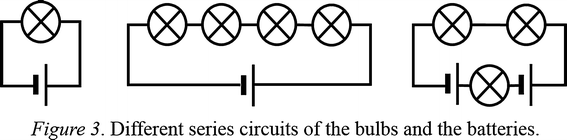

  

  Figure 3 in the laboratory report of group 5

• Figure 2. Estimating the differences of currents through comparing the brightness of the bulbs.

• 1. (d) The electric circuits in Figure 3 (see Fig. 5) can be used for explaining to students that the amounts of bulbs and batteries affect the magnitude of current but their order does not matter.

Connecting different amounts of bulbs in series in a way presented in Figure 3 (see Fig. 5), it can be observed that they turn off and on simultaneously, and they burn equally bright. Thereby, a current of the same magnitude flows through them. The more bulbs are connected in series, the dimmer they burn. It can also be noticed that adding voltage sources in series makes the bulbs burn brighter. Therefore, the magnitude of current depends on the amount of batteries. In the series circuits, the order of the components does not affect the electrical properties of the direct current circuit.

• 1. (e) The circuit in Figure 4 (see Fig. 6) can be used for reifying to students how the electric current divides when the circuit branches and how the magnitude of current changes when it goes through two routes at the same time. When the switch in Figure 4 (see Fig. 6) is closed, the current divides in two branches. There is now a parallel connection between two bulbs, which have smaller brightness than the third bulb of the circuit because the total current goes through it.

  Fig. 6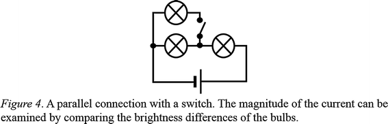

  

  Figure 4 in the laboratory report of group 5

The quantification of the electric current

• 1. (f) In this experiment, a quantity that describes the magnitude of electric current is introduced to students. The meaning of the new quantity is defined to be proportional to the measurable property of the phenomenon’s effect.

The experiment is done applying magnetic interaction. The setup of experiment is presented in Figure 5. Similar bulbs are connected in parallel. The brightness of the bulbs is the same; therefore, same amount of current goes through the bulbs. A coil is connected as a part of the electric circuit so that the current in coil is always the same as the current through the chosen bulbs, which are connected in parallel. The current can be connected through one, two, three, four or five bulbs. Thus, the current in coil correlates with the current through the certain bulbs. The magnetic force in the coil caused by the electric current is measured by putting a bar magnet on scale, and the coil attracts the magnet upward. The force can be determined in a static situation by balancing the scale every time when the attraction of the coil changes due to different bulb configurations. Thus, it can be observed that the interaction of magnetic force is linearly proportional to the magnitude of electric current.

• [See Fig. 1]

• Figure 5. Diagram of the quantifying experiment of current.

• [Photo of the measurement system]

• Figure 6. The measurement, where the current in the coil goes through all five bulbs.

The resistance in the coil has to be a constant, i.e., not depending on the current. In other words, it cannot warm up so that it would not change the current flowing in the circuit in different circumstances. Hence, the cross-sectional area of the conductor has to be big enough, and it has to have limited amount of turns.

The bar magnet has to be in same position in relation to the coil in every measurement that the shape of the magnetic field does not affect in the measurement of the force. In Table 1 (see Table 5), the measured values are presented. In Figure 6, the measurement system is presented. In Figure 7 (see Fig. 7), the magnitude of force is presented as a function of currents of the bulbs.

Table 5 Table 1 in the laboratory report of group 5 with the text: “Numerical values of the quantifying experiment of the electric current”

Fig. 7

Figure 7 in the laboratory report of group 5 with the text: “The force as a function of current behaves linearly.”

Because the electric current is now quantified, we can start to use ammeters, whose measurements are based on the measurement of the magnetic force caused by the electric current.

References

Chang, H. (2001). Spirit, air, and quicksilver: The search for the “real” scale of temperature. Historical Studies in the Physical and Biological Sciences, 31(2), 249–284.
Hacking, I. (2008). Representing and intervening. Cambridge: Cambridge University Press.
Hanson, N. (1958). Patterns of discovery. Cambridge: Cambridge University Press.
Jammer, M. (1961). Concepts of mass in classical and modern physics. Cambridge: Harvard University Press.
Koponen, I. T., & Mäntylä, T. (2006). Generative role of experiments in physics and in teaching physics: A suggestion for epistemological reconstruction. Science and Education, 15, 31–54.
Kuhn, T. (1961). The function of measurement in modern physical science. Isis, 52(2), 161–193.
Kurki-Suonio, K. (2011). Principles supporting the perceptional teaching of physics: A “practical teaching philosophy”. Science and Education, 20(3–4), 211–243.
Mäntylä, T. (2013). Promoting conceptual development in physics teacher education: cognitive-historical reconstruction of electromagnetic induction law. Science and Education, 22(6), 1361–1387.
Mäntylä, T., & Koponen, I. T. (2007). Understanding the role of measurements in creating physical quantities: A case study of learning to quantify temperature in physics teacher education. Science and Education, 16, 291–311.
McDermott, L. C., & Shaffer, P. S. (1992). Research as a guide for curriculum development: An example from introductory electricity. Part I: Investigation of student understanding. American Journal of Physics, 60(11), 994–1003.
Smith, C., & Wise, M. (1989). Energy and empire: A biographical study of lord Kelvin. Cambridge: Cambridge University Press.
Steinle, F. (1997). Entering new fields: Exploratory uses of experimentation. Philosophy of Science, 64, S65–S74.
Thomson, W., & Tait, G. (1867). Treatise of natural philosophy (Vol. I). Oxford: Clarendon press.
Trumper, R. (2003). The physics laboratory—A historical overview and future perspectives. Science and Education, 12, 645–670.
Tweney, R. (2012). On the unreasonable reasonableness of mathematical physics—A cognitive view. In R. Proctor & E. Capaldi (Eds.), Psychology of science (pp. 406–435). Oxford: Oxford University Press.
Uhden, O., Karam, R., Pietrocola, M., & Pospiech, G. (2012). Modelling mathematical reasoning in physics education. Science and Education, 21(4), 485–506.
Whewell, W. (1840). The philosophy of the inductive sciences founded upon their history (Vol. 1). London: Harrison & co.
Acknowledgments
This work was supported by the Academy of Finland through Grant SA257400.
Author information
Authors and Affiliations
Corresponding author