
Abstract
Hadoop is a software framework allowing for the possibility of coding distributed applications starting from a MapReduce algorithm with very low programming efforts. However, the performance of the implementations resulting from such a straightforward approach are often disappointing. This may happen because a vanilla implementation of a MapReduce distributed algorithm often suffers of some performance bottlenecks that may compromise the potential of a distributed system. As a consequence of this, the execution times of the considered algorithm are not up to the expectations. In this paper, we present the work we have done for efficiently engineering, on Apache Hadoop, a reference algorithm for the Source Camera Identification problem (i.e., determining the particular digital camera used for taking a given image). The algorithm we have chosen is the algorithm by Lukáš et al.. A first implementation has been obtained in a small amount of time using the default facilities available with Hadoop. However, its performance, analyzed using a cluster of 33 PCs, was very unsatisfactory. A careful profiling of this code revealed some serious performance issues targeting the initial steps of the algorithm and resulting in a bad usage of the cluster resources. Several theoretical and practical optimizations were then tried, and their effects were measured by accurate experimentations. This allowed for the development of alternative implementations that, while leaving unaltered the original algorithm, were able to better use the underlying cluster resources as well as of the Hadoop framework, thus allowing for much better performance and reduced energy requirements than the original vanilla implementation.
1 Introduction
The ubiquitous presence of sensors in people’s everyday-life yields day-by-day a huge amount of data which need to be gathered, structured and processed by decision making systems. The technologies provided by the big data processing based tools make it possible to manage and analyze this data in an efficient and scalable way. The areas which have mostly taken advantage from this new real world scenario are those connected to the security, like biometric recognition, crowd analysis and video surveillance systems, and especially related to the Digital Image Forensics [5, 14, 18, 22]. In recent literature, including both educational books and scientific papers, many solutions applied to real world problems are available. As the use of smartphones and portable devices increases, together with the digital photography and quick systems for scene representation and shooting, there is the need to further analyze how the scale issue is managed by these solutions, also by exploring their optimisation advantages (or disadvantages) when migrated on distributed systems [10, 25]. In order to solve the Source Camera Identification (SCI) problem, in the here proposed paper (prosecution of a previous approach described in [7]), we have developed a distributed version of the algorithm by Lukáš et al. [18] based on the MapReduce paradigm and implemented using Hadoop. SCI represents the topic of interest; it deals with the recognition of the camera used for the acquisition of a specific digital image [13], an issue which plays a fundamental role in the Digital Image Forensics topic [3], with sensitive consequences in biometric recognition [2, 20] and video surveillance [21]. In an initial implementation, the standard facilities of Hadoop have been exploited in order to develop a distributed code which, although showing low execution times when executed on clusters of computers, exhibited performance below the expectations. Further analysis, that have been conducted on this initial approach, have revealed performance issues tightly related to the inability of fully exploiting the underlying resources of the cluster. These issues cause a significant waste of CPU cycles as well as the occurrence of long periods of heavy data traffic on the underlying network thus resulting in longer execution times and abnormal power requirements. The new implementation proposed in this work focuses on the causes behind the performance issues observed; therefore, these have been solved by means of the introduction of both theoretical and practical optimization algorithms which produced performance results much better than those yielded by the original implementation.
The remaining of this paper is organized in the following way. First, the MapReduce paradigm is described in Section 2, also with a deep look to Apache Hadoop. Sections 3 and 4 present the algorithm by Lukáš et al., which represents the case study we focused on and how it has been ported over a Hadoop cluster. Section 5 shows the preliminary experimental results. Section 6 poses the focus on the performance issues exhibited by our distributed implementation; also, further improvements are proposed and analysed. Finally, in Section 7 we discuss some conclusions of our work.
2 Big data processing
A wide variety of technological and architectural solutions for big data processing have been proposed over recent years. Among other paradigms, MapReduce [10] gained increasingly attention. It was introduced by Google, that adopted it with big success for the processing of big data, offering scalability, parallel computing and tolerance to faults, and is used nowadays in a wide range of application fields (see, e.g., [4, 9, 11, 12, 16, 19]). In the following, this paradigm is briefly reviewed together with Apache Hadoop, its most popular implementation.
2.1 MapReduce
The MapReduce computing paradigm is based on a set of input < key,value > pairs that are turned into a set of output < key,value > pairs. Each input pair is given to a map function that generates a set of intermediate < key,value > pairs. Once all intermediate pairs are generated, the MapReduce framework collects and groups them according to equal value of intermediate key. Then, such groups are given as input to the reduce function. As its name suggests, each reduce function aims at merging the intermediate values in a smaller, possibly the smallest, set of values. Usually, one output pair, or even no pair, is generated per reduce function.
Map and reduce functions are computed as tasks on the nodes of a distributed system. MapReduce differs from traditional paradigms since it allows for implicit parallelism. Rather than implementing an explicit parallelism based on message-passing, in MapReduce a file-based approach relates all operations involving data exchange between nodes. The underlying middleware transparently accomplishes such a task. On the other hand, the MapReduce framework directly controls all other aspects like load balancing and the use of the network, distribution and replication of data over the distributed architecture, scheduling and synchronisation and so on.
2.2 Hadoop
It is one of the most popular frameworks for the implementation of MapReduce-based distributed applications. It mainly consists of a Hadoop Distributed File System (HDFS) and a computing framework [24]. Input files are read and organized by the framework as a set of < key,value > pairs. The nodes of the computing cluster (i.e., slave nodes) run the Hadoop containers that, in turns, run the tasks. Each task is in charge of running a user-defined map or reduce function on a set of input pairs. Input files are first partitioned in blocks and then distributed and replicated on the nodes of the cluster. All these blocks are replicated several times on different nodes according to a replication factor. Whenever a task does not process a block in the expected time, the same task is issued on another node containing a replica of that block, then the first task to complete will be kept while the other one will be killed (i.e., speculative execution).
One of the main advantages of Hadoop is about its easiness of use. The developer is only asked to define the behaviour of the map and reduce functions. All the other activities are transparently carried out by Hadoop. This advantage comes at a cost as, when solving a particular problem, the standard strategies employed by Hadoop for performing these activities may not be the best ones. This is especially true for all data-management activities, as these are performance-critical in a distributed application. The consequence is that MapReduce algorithms that are theoretically very efficient may perform very bad when implemented over Hadoop without any particular engineering activity.
This problem can be partially solved by overriding the standard Hadoop data-management features. A brief description of the Hadoop features customized for our purposes is presented below:
Sequence Files. The generation of a big amount of small files is a known performance problem of Hadoop, mainly due to some indexing issues (see [26]). Sequence files can be used in Hadoop to overcome such a limitation. These are binary files whose format can be customized by the developer. They also allow for the definition of a custom split strategy so that their content can be properly partitioned on the different slave nodes of a Hadoop cluster and processed locally so to achieve data local computation. Used in our proposal to significantly reduce the time required to process batch of images.
Distributed Cache. It is quite common for a complex Hadoop application to require an input file to be spread to all the slave nodes at the beginning of the computation (e.g., using a dictionary of relevant words during the execution of a topic-extraction model). Such a task can be efficiently accomplished through the usage of the DistributedCache. Used in our proposal to optimize identification times by caching the fingerprint of each digital camera under scrutiny on each node of the distributed system.
Combiner. Hadoop algorithms generating a large number of small intermediate < key,value > pairs may perform poorly because of the significant network and the I/O overhead required to manage these pairs in contrast with their small size. To overcome this problem, Hadoop allows for the definition of a Combiner function useful to aggregate in-memory the multiple output pairs of map tasks in a (possibly) smaller number of pairs, thus reducing the network and I/O overhead. Used in our proposal to significantly reduce network traffic by aggregating the residual noise extracted from a batch of images taken with a same camera.
3 The case study: the algorithm by Lukáš et al.
Recovering the identity of a digital camera from the digital images taken by it is a problem commonly known as Source Camera Identification (SCI). A typical strategy consists in finding clues of a specific digital sensor by analyzing the noise in the digital image. Noise in a digital image refers to the presence of color distortions, at pixel level, that are not present in the grabbed scene and, hence, should not appear in the image. Such a noise can be random (i.e., Shot Noise) and/or deterministic (i.e., Pattern Noise). The second type of noise can in turn be divided into: (i) the Fixed Pattern noise (FP) and (ii) the Photo-Response Non-Uniformity noise (PRNU). Both relate to the amount of light that the pixel detectors can grab but they are opposite each other. The FP noise is caused by the information received by pixel detectors in absence of light (dark currents). The PRNU noise is mostly due to the Pixel Non-Uniformity noise (PNU noise) which is caused by the sensitivity of the detectors to the light received. Due to inhomogeneities of silicon wafer and imperfections occurring at manufacturing time, it happens that pixel detectors catch light differently from expected, thus introducing noise. Reasonably, the random component of noise does not help in solving the SCI problem. On the other side, the systematic and deterministic side of PNU noise makes it possible to consider it as a kind of fingerprint of digital cameras.
For example, Kurosawa et al. [17] were able to identify the camcorder used to record a video from dark current noise in videotaped images. Lukáš et al. in [18] pioneered this field of research demonstrating the PNU noise acting as a feature for feasible solution in SCI problem. They showed how the PNU noise can be used to identify and distinguish a camera from another, even when considering different cameras of the same model. Significant results have been also obtained on post-processed images, like those subjected to JPEG compression, re-sampling, gamma correction and filtering.
Source Camera Identification techniques have also been explored on large datasets. The work by Fridrich et al. in [14] represents the main contribution on this area. Over one million images have been tested, captured by a high number of different cameras, that is 6,896, from 150 different models. Another relevant result has been obtained with cameras embedded in mobile devices. An experiment on a dataset containing images taken from 2,000 iPhones was presented in [15], proving the power of a fast searching algorithm based on fingerprint digests.
Our work is applied to color images in RGB space and was inspired to the original version of the SCI algorithm by Lukáš et al. [18]. Let CamSet = {C1,C2,…,Cn} be the set of classes, defining all possible cameras available in the dataset, and I be the RGB grabbed from one of the cameras in CamSet. The algorithm consists of four steps:
Step A: Computing the Reference Patterns. For each camera C in CamSet, generate the reference pattern RPC as the sensor fingerprint of that camera C. Following the proposal by Lukáš et al., the reference pattern is estimated by the Residual Noise (RN) from a set of pictures taken by the C camera and combining the individual residuals together to form the best approximation for the PNU noise of the sensor considered. Given an image I, the residual noise is computed as RNI = I − F(I), where a filter function F(I) returns the noise-free variant of I. This operation is performed at pixel level, for each channel, and iterated over a collection of K equal spatial resolution images taken by the same camera C, hereafter mentioned as enrollment images. The K noises obtained, including both the estimation of the PNU and the random component of the noise are summed up and averaged over the K images considered, thus providing a tight approximation RPC of the fingerprint of the camera C (see (1)).
$$ RP_{C} = \frac{{\sum}_{k=1}^{m} RN_{k}}{m}. $$(1)The pseudo-codes of the map and reduce functions of this step are illustrated in Algorithm 1.
Step B: Computing the Correlation Indices. Two subsets of images per camera in CamSet are introduced: (i) the calibration set and (ii) the testing set. For each camera C and the residual noise RNT of the image T taken from CamSet, the Pearson’s correlation index is computed, according to (2). High correlation values indicate that the T image has likely been acquired by the sensor of C. Resolution of T is adjusted, by cropping or resizing the image itself, in case it does not match with the resolution used to compute the reference pattern of that camera RPC.
$$ corr(RN_{T}, RP_{C})= \frac{\left( RN_{T} - \overline{RN_{T}}\right)\left( RP_{C} - \overline{RP_{C}}\right)}{\left|\left|RN_{T} - \overline{RN_{T}}\right|\right|~~\left|\left| RP_{C} - \overline{RP_{C}}\right|\right|}. $$(2)The pseudo-code of this step is illustrated in Algorithm 2.
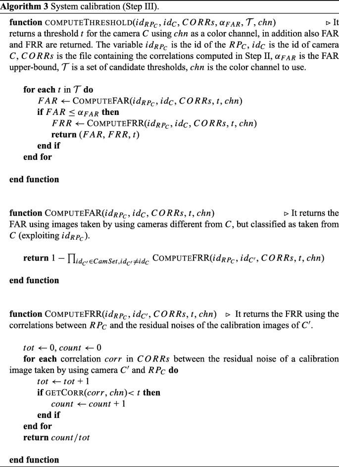
Step C: Calibrating the Identification System. For each camera a triple of identification thresholds, one per color channel, is empirically defined. An image I is said to have been taken from the camera C if, for each color channel, the correlation between the Reference Pattern of the camera and the residual noise of the image is greater than the corresponding threshold for that color channel. The thresholds are empirically defined according to Neyman-Pearson approach. That is, the False Rejection Rate (FRR) for calibration images taken by using C is minimized given an upper bound on the False Acceptance Rate (FAR) for calibration images taken by using a camera different than C. The correlations of the testing images are then used to validate the identification system by comparing them to the acceptance thresholds.
The pseudo-code used for computing the threshold for a camera C is illustrated in Algorithm 3. The function computeThreshold is iterated for each camera and color channel.


Step D: Source Camera Identification. It represents the final stage of the algorithm, that is the identification of the camera C that captured I. The residual noise from I, RNI, is first derived. Then, the correlation with Reference Patterns of all cameras is computed according to calibration performed in step C. A match is found with that camera C for which the highest correlation that exceeds the triple of thresholds is achieved.


4 A naive implementation of the algorithm by Lukáš et al. on Hadoop
We implemented the algorithm by Lukáš et al. by using the MapReduce paradigm.Footnote 1 It was entirely written in Java including the filter described in the previous section. The code has been arranged in four different packages, one for each processing steps of the algorithm by Lukáš et al..
First the images are fetched from the HDFS. No extra work was necessary because the input dataset was represented by a set of jpeg files in the same directory. In the following paragraphs the four packages are described in details.
Step I: Reference pattern extraction
During the execution of this step, a set of enrollment images is processed. The output produced is the reference pattern of CRPC. It is assumed that all the images have been produced by the same camera C and have the same resolution. The input is split by the resource manager among all the available Hadoop containers. Therefore, each map task processes a set of images for extracting their residual noises. These are, in turn, sent to the reduce tasks. In the reduce phase, all the residual noises of a given camera C are combined by computing the average for each pixel value. When all the residual noises have been processed, the resulting reference pattern is stored on HDFS. As consequence, the number of reduce tasks is identical to the number of input cameras (see Algorithm 1).
Step I takes as input a list of < key,value > pairs. Here, the key reports some meta-data about the image being loaded and value holds the input image path (URL) on HDFS. For each element of this list the map function is called, the corresponding image is loaded in memory from HDFS and than it is processed to extract the residual noise. A new < key,value > pair is produced as output, where key is the identification number of the camera and value is the path (URL) where the residual noise has been stored on HDFS.
Similarly, the reduce tasks receive as input a list of < key,values > pairs, where key holds the identification number of the camera C, and values is the list of the URLs where the residual noises for that camera have been saved on HDFS by the map tasks. Then, the Reference Pattern RPC for the camera C is computed as the average of all the residual noises extracted from the images produced by C. The final result is produced as list of < key,value > pairs, where key is the identification number of C and value is its reference pattern.
Step II: Processing correlation indices
When all the reference patterns have been computed, as next step, a set of testing/calibration images is processed, extracting the residual noise. Each residual noise is compared against the reference patterns of all the considered cameras by means of the correlation index.
The map phase starts with a list of < key,value > pairs addressing the input images to be processed, where key derives from the image meta-data and value is the path on HDFS of the image. For each pair, if the image is originally stored on a different node, it will be automatically transferred by Hadoop to the node that will run the task. The image then is filtered and the resulting residual noise is correlated with each reference pattern computed in the previous step. For each correlation index (obtained comparing the input residual noise against one of the reference patterns), the map function produces on the output channel a new pair with key equal to the string “Correlation” and value equal to the string obtained by concatenating the following values: the image id, the camera id which produced the image, the RP id, the correlation preprocessing type and, finally, three correlation indices (one for each color channel). Before starting the processing, each slave must load all the reference patterns. In order to speedup this operation, the Hadoop DistributedCache mechanism has been applied to force each node to transfer in advance to its local storage a copy of these files, before executing the real Hadoop job. This step does not require any further computation and therefore no reduce task is started (see Algorithm 2).
Step III: System calibration
For each of the input cameras three acceptance thresholds must be computed, one for each color channel, before the system is ready. According to the Neyman-Pearson approach, these thresholds can be determined starting from the correlation values computed in the previous step for a set of classified images used only for calibration purposes (calibration set). Additionally we consider the correlation values of another set of images (test set), again produced during the execution of Step II. These values are used to measure the performance of the identification system. In fact, these values are compared to the three thresholds just defined. This step is computationally light and, therefore, it is sequentially executed only on the master node (see Algorithm 3).
Step IV: Source camera identification
In this step it is established which camera (among those considered in the previous steps) has been used for acquiring a given image I. The Hadoop job reads the input from the same folder where the reference patterns have been stored and then it writes on the output the id of the camera with the reference pattern recognized to be the closest to the residual noise included in the image I. With this goal in mind, for each input reference pattern, a new map function is run on an instance of I. It will be filtered extracting its residual noise and a new correlation index will be computed comparing the residual noise with the input reference pattern.
As result, the job produces the list of the correlation indices. These will be used to start the recognition phase applying the same thresholds computed in the previous step. As a result, it will be returned the identification number of the camera with the highest index. The workflow of the algorithm is depicted in Fig. 1.

The overall schematic view of the workflow describing the Naive implementation we developed of the algorithm by Lukáš et al.
5 Experimental analysis
The performance of the proposed algorithm have been assessed by means of an experimental analysis. Namely, its performance have been compared with the ones of a sequential implementation of the algorithm by Lukáš et al.. The results of this experimentation as well as a discussion of the experimental settings are provided in the rest of this section.
5.1 Experimental settings
We conducted our experiments on a computing cluster of 33 identical workstations. Each workstation featured an Intel Celeron G530 dual-core processor, 4 GB of RAM and was running the Linux operating system. The Hadoop setup included 32 slave nodes and one master node running the standard Hadoop services. Due to the limited amount of available memory, each slave node was configured to run at most one map task and/or one reduce task at time. The HDFS file system was configured with a replication factor of 2 and a standard block size set to 64 MB.
We considered for our experiments the same dataset chosen in [6], and consisting of 5, 160 4288×2848 JPEG images, taken using 20 different Nikon D90 cameras, for a total size of about 20GB. For each of these cameras, 258 images were taken at the highest possible resolution while using a very low JPEG compression degree. These were then organized in 64 calibration images, 64 testing and 130 enrollment images for each camera. These last images portray a ISO Noise Chart 15739 [23], while the other images portray various types of scenes (see Fig. 2 for an example). We remark that noise charts images have been used for enrollment as they have been purposedly designed for noise extraction. Instead, the heterogeneity of subjects portrayed by calibration and testing images makes it more difficult to extract the PNU noise of their corresponding digital cameras.

Two example scenes used for calibration and testing purposes
5.2 Preliminary experimental results
Our experimentations led to the development of a sequential implementation of the algorithm by Lukáš et al. (i.e., SCI), plus several different distributed variants of the same algorithm. In our preliminary experimentation, we take into account the first distributed variant we developed, HSCI(i.e., Hadoop SCI). It is a literal implementation of the algorithm described in Section 4. At this stage, we focus on Step I and Step II of this algorithm, as these are, indeed, the most computationally demanding.
At beginning of Step I, all the input images are loaded on the HDFS file system. Notice that also the files containing the residual noises and the reference patterns, resulting from the execution of the different steps of the algorithm, are saved on HDFS. So, for performance reasons, the map and reduce tasks implementing the algorithm will take as input and return as output not the image themselves, but their HDFS URL address.
In our first experiment, we compared the performance of HSCI with those of SCI, when run on a single node of our computing cluster. During this experiment, we measured the overall execution time of each step of the algorithm. The results of this experiment, reported in Table 1, indicate that the distributed implementation of the second step of the algorithm is about 16 × faster than its sequential counterpart. Surprisingly, instead, the first step of the algorithm does not seem to benefit from its distributed execution. This behaviour seems to be due to a performance bottleneck found in the reduce phase of this step. As a matter of fact, in order to run, the first step reduce phase requires each task to retrieve a large set of residual noises generated during the map phase (e.g., in our case, each reduce task had to collect 130 residual noises having each a size of about 140 MB). Consequently, the running time of this phase is dominated by the time required to load these files.
This circumstance has been further confirmed by profiling the resource usage of HSCI during its execution. The results show that the CPU is mostly unused while the tasks spend most of their execution time to perform network related operations. A possible optimization to mitigate the aforementioned problem could be to reduce the number of files to be processed and to better exploit data local computation by placing data on the same nodes where they have to be processed. To implement this solution, we encoded all input images using just two very large Hadoop SequenceFile objects to contain them. The first is the EnrSeq sequence file and it is used for storing all the enrollment images. The second is TTSeq sequence file and it is used for maintaining the calibration and the testing images. In both cases, the order used to sort the contained images in their corresponding sequence files is the one of their originating camera id. Once packed all the image files in these sequence files, we used the input split capability provided by Hadoop to break each sequence files in blocks to be distributed among the slave nodes of the cluster, with each node in charge of processing its own blocks. The implementation of this strategy (i.e., HSCI_Seq) led to a significant performance improvement in the first step of the algorithm, allowing for an execution time that is about 2.6 × faster than the previous implementation. Even the second step of the algorithm experiences a performance gain thanks to this optimization, even if relatively small.
6 Advanced experimental analysis
The experiments discussed in the previous section highlighted that the performance of our vanilla distributed implementation of the algorithm by Lukáš et al. is affected by the heavy network activity required to retrieve and to store the residual noises on HDFS. We tackled this problem by first profiling the performance of HSCI_Seq, to better understand the reasons behind this performance bottleneck. Then, we introduce some other optimizations to further improve the performance of this algorithm.
6.1 Profiling HSCI_Seq implementation
As described in the previous section, our HSCI_Seq implementation is able to optimize the performance of the algorithm by Lukáš et al. thanks to the usage of two sequence files. When processing our reference dataset, this strategy implies the processing of about 8GB for a total of 130 map tasks. According to our profiling, this translates in about 355 GB of shuffle data transmitted by map tasks to reduce tasks. On the reduce side, the number of tasks to run has been set to 20, roughly corresponding to the number of RP s to extract. On this matter, our profiling revealed that over the 75% of the Step I HSCI_Seq running time was spent in the reduce phase. Indeed, much of this time is spent retrieving all the residual noises files from the underlying storage system. However, this overhead is also due to the time required for processing and aggregating these residual noises, once they have been loaded in memory. Finally, we also noticed that several map and reduce tasks were killed during their execution.
To further analyze these phenomena, we traced the lifetime of each task run by HSCI_Seq on our reference dataset, starting from the moment it was scheduled up to its conclusion. We report a focus on these traces when considering the Step I of HSCI_Seq in Fig. 3. Notice that Hadoop may choose to replicate on different slave nodes those tasks taking too much time with respect to their expected execution time. When this happens, once the first replica of a task ends, all the other replicas are killed without waiting for their conclusion. Such cases are highlighted in our figure by coloring black all the tasks that have been killed for this reason. By looking at this figure, it is clear that map tasks are evenly balanced among all nodes of our cluster as they do all have a similar execution time. Speaking of the reduce tasks, we notice the existence of some tasks having a very short lifetime. These are tasks that have been issued without having any RP to calculate.

HSCI_Seq implementation - A timeline of the map and reduce tasks run while executing Step I
With the previous profiling, we analyzed the lifespan of the tasks issued while running HSCI_Seq. As a further step, we analyzed the inner behaviour of these tasks by focusing on their CPU usage and network activity. For example, we report in Fig. 4 the CPU activity of a generic slave node. As it can be clearly seen, about the first 60 minutes are spent executing map tasks. In this phase, the CPU is used almost at its maximum, thus suggesting that map tasks have been very busy running user code. When turning to the second phase, the situation completely changes, as reduce tasks take approximately the same time required by map tasks, but using a very small amount of CPU. This is a further confirmation that most of the time required by the Step I reduce phase is spent while waiting for network activities to complete. This is even confirmed by looking at the incoming network throughput for a generic slave node during Step I, as described in Fig. 5. Indeed, there is a relevant network activity for these nodes during the map and the reduce phases.

CPU usage of a slave node when running Step I of HSCI_Seq, expressed in percentage

Incoming network throughput of a slave node, in MB/s, when running Step I of HSCI_Seq
When turning to Step II, we notice that at least 194 map tasks have to be run for processing the testing and the calibration images existing in the TTSeq sequence file. In our profiling experiment, 210 map tasks were automatically run, with 16 tasks being killed by Hadoop due to speculative execution. Moreover, of these tasks, 187 were run on locally available data while the remaining ones processed an HDFS data block initially found on a different node. Consider that the second step of HSCI_Seq does not run any reduce task, so its execution time can be approximated to that of the map phase. By profiling these map tasks, we found that their behaviour is characterized both by an intense I/O activity and CPU activity. The first can be explained by considering the overhead to be payed for loading in memory the Reference Patterns from a remote location. The latter are due to the work needed for correlating the different images (see Fig. 6). It is interesting to note that, during this phase, the average CPU usage is far from the maximum (e.g., around 40%). We also observe that the CPU is idle along the initial part of this step, roughly corresponding to the time required for Hadoop to copy the RP s from HDFS to the local storage. On a side, this opens to the possibility of running two tasks on the same node, as each task uses less than half of the available CPU power. On the other side, we recall that, in our setting, each node does not have enough memory to run two tasks in parallel.

CPU usage of a slave node when running Step II of HSCI_Seq, expressed in percentage
6.2 Further optimizations and results
The results of the profiling activity we just described allowed us to determine two performance issues affecting HSCI_Seq. These have been characterized and, then, solved by introducing some proper practical optimizations.
Excessive network traffic
The volume of data required to transfer a significant number of residual noises from nodes where map tasks are run to nodes where the corresponding reduce tasks will be run give rises to a large amount of network traffic. In order to mitigate this problem, we introduced an aggregation strategy on the map-side to combine all the residual noises generated by a same map task and related to a same camera into one single residual noise file. This allows to transfer a batch of residual noises as they were one single residual noise file. The aggregation is obtained through a numerical sum of all the residual noise files produced by a task for a same camera. To facilitate this operation, the partial sum of the residual noise files is maintained in memory by the node, this allows to save the time otherwise spent for saving these files on the local storage and loading them back. In a first attempt, we implemented this mechanism using the standard Hadoop Combiner. However, its results were disappointing because it required to maintain in memory a copy of all residual noises files before summing them. This would easily consume all the memory available on a node, thus leading to a crash of the application. To overcome this problem, we implemented a different solution based on a custom aggregation strategy able to store in memory not all the residual noise files, but only their sum (i.e., in-map aggregation). Moreover, we used a feature available with Hadoop for straightly returning this sum as a (key,value) output pair, instead of saving it on HDFS. We called HSCI_Sum the variant of HSCI_Seq including this optimization.
Poor CPU usage
As observed during our profiling, the current definition of the map phase run during Step II requires an intense CPU activity to be fulfilled. However, its formulation is strictly sequential and it is unable to exploit the availability of any additional CPU cores, like in our case. In details, the map phase can be logically divided in two parts. In the first part, the reference pattern file of a particular camera is loaded from the local file system. In the second part, the correlation of the outcoming file with an input residual noise is calculated. So, the first part is mostly I/O bound while the second part is CPU bound. In order to speed-up this phase and take advantage of any additional CPU cores, we modeled it after the producer-consumer paradigm and implemented it as a multi-threaded application. We thus defined two threads to be run in parallel. The first thred is in charge of retrieving from the local storage the reference pattern files and store them in a shared-memory queue. The second thread keeps waiting until a reference pattern file is saved in the shared-memory queue, retrieves it and, then, evaluates its correlation with respect to a target camera residual noise. We added this optimization to HSCI_Sum, thus obtaining HSCI_PC.
Unbalanced partitioning
The standard reduce partitioning strategy implemented by Hadoop, when used for allocating reduce functions according to the camera id (as required by Step I of HSCI_Seq) with a number of cameras smaller than the number of slave nodes, may assign multiple functions to a same slave node while leaving other slave nodes without functions to process. We overcome this problem by introducing a custom partitioner featuring a perfect hash function, so that wherever the number of slave nodes is higher than the number of cameras, no single node would be assigned to more than one reduce function at time. This function maps distinct keys (i.e., camera id) on a set of integers so to guarantee a more balanced partitions. For instance, in our case, the adopted function guarantees that each node will process either none or one RP. The implementation of this strategy, here denoted HSCI_All, also includes the optimizations introduced by HSCI_Sum and HSCI_PC.
Once implemented all the optimizations described so far, we compared the performance of the resulting distributed applications with the sequential Lukáš et al. implementation (HSCI). As witnessed by Table 2, these new implementations are more efficient than HSCI_Seq. For example, HSCI_Sum is significantly faster than HSCI_Seq when running the first Step of the algorithm by Lukáš et al.. This performance gain has been obtained thanks to the strategy featured by HSCI_Sum to aggregate residual noises, thus drastically reducing the volume of data exchanged between map and reduce tasks.
We also observe that a smaller amount of data to be exchanged not only implies short communication times but also a smaller number of task replications, because of the reduced probability of network congestions. In addition, the execution time of the reduce phase is very short.
When turning to the Step II of the algorithm by Lukáš et al., we notice that the introduction of the producer-consumer paradigm as well as a multi-threaded architecture allows for a consistent performance gain, as witnessed by the performance of HSCI_PC. This if further confirmed by the consistent increase in CPU usage of HSCI_PC measured when running the map phase of Step II and described in Fig. 7, with respect to the usage profile of HSCI_Seq (see Fig. 6).

CPU usage of a slave node when running Step II of HSCI_PC, expressed in percentage
Finally, we consider HSCI_All . This algorithm uses a custom partitioner to ensure that, in our setting, two reduce functions cannot be assigned to a same slave node during Step I, while leaving other nodes unused (unless duplicate tasks) . Even in this case, we noticed a slight performance improvement on HSCI_Sum during Step I (48 minutes against 49 minutes), though smaller than we expected (Fig. 8). A closer investigation revealed that, on one side, the custom partitioner was able to avoid the assignment of two different reduce functions to a same node (see Fig. 9), and that, on the other side, the stack of optimizations decreased the average execution time of the reduce functions so much that the effects of this last optimization were quite negligible.

Efficiency of HSCI_All compared to SCI when running on a cluster of increasing size (n is the number of slave nodes)

HSCI_All variant - An overview of map and reduce tasks launched during Step I. Notice that reduce tasks start only after the termination of all map tasks
6.3 Scalability test
In this last round of experiments, we investigated the scalability of HSCI_All compared to its sequential counterpart, i.e., SCI.
We considered for our study just the computational heavier steps of the algorithm by Lukáš et al., i.e., Step I and Step II. Scalability has been measured by progressively increasing the size of the cluster from 4 up to 32 slave nodes and, then, measuring the efficiency of HSCI_All compared to that of SCI according to the following formula:
In (3), n is the number of slave nodes of the cluster, TSCI and \(T_{\texttt {HSCI\_All}}(n)\) are the execution times of SCI and HSCI_All, respectively, when run on a cluster of size n. The results are available in Table 3, Figs. 8 and 10. We observe that, as the cluster size increases, the performance improvement for Step I gets smaller than the one achieved by Step II. This drawback is due to the fact that, when processing the reduce phase of Step I using 32 slave nodes, only 20 of these are employed (since 20 is the number of RP s to be calculated).

Speed up of HSCI_All compared to SCI when running on a cluster of increasing size.
7 Conclusion
The goal of this paper has been the introduction of a distributed version of the source camera identification algorithm by Lukáš et al., reformulated according to the Hadoop framework. We started from a vanilla implementation of the algorithm that has been then subject to a careful experimental analysis in order to pinpoint potential performance issues. These have been further characterized through a deep profiling activity. As a results, we developed and tested several theoretical and practical optimizations of the original algorithm by Lukáš et al. Our experimental results show that these optimizations succeed in significantly improving the performance of the original algorithm, thus allowing to obtain a consistent speedup with respect to the sequential implementation of the algorithm, when run on a Hadoop computing cluster of 32 slave nodes.
As a more general consideration, we observe that the availability of software frameworks and algorithmic solutions able to process big volumes of data in a reasonable amount of time is a pressing problem in a wide range of applications areas like the analysis of large collection of genomic sequences in bioinformatics (e.g., [4, 11, 12]) or the management and the fast reconfiguration of 5G cellular networks (e.g., [1, 8]). To this end, we observe that frameworks like Hadoop or Spark are attractive because of the possibility of coding distributed applications in a very small amount of time and without requiring complex programming skills.
However, as witnessed by our case, this simplicity comes at a cost, as a straightforward implementation of a distributed algorithm by means of these frameworks may result in an application code that is inefficient and unable to fully exploit the available computing resources. Indeed, in these cases it is very helpful to adopt a proper algorithm engineering methodology able to measure how efficiently a theoretical algorithm is translated and executed on a real distributed computing facility, and which actions may be taken in order to improve this efficiency.
Notes
A copy of this code is available upon request.
References
Amorosi L, Chiaraviglio L, D’Andreagiovanni F, Blefari-Melazzi N (2018) Energy-efficient mission planning of uavs for 5g coverage in rural zones. In: 2018 IEEE international conference on environmental engineering (EE), pp 1–9. https://doi.org/10.1109/EE1.2018.8385250
Barra S, Casanova A, Fraschini M, Nappi M (2017) Fusion of physiological measures for multimodal biometric systems. Multimed Tools Appl 76(4):4835–4847. https://doi.org/10.1007/s11042-016-3796-1
Barra S, Fenu G, De Marsico M, Castiglione A, Nappi M (2018) Have you permission to answer this phone?. In: 2018 international workshop on biometrics and forensics (IWBF), pp 1–7. Institute of Electrical and Electronics Engineers Inc. https://doi.org/10.1109/IWBF.2018.8401563
Cattaneo G, Ferraro Petrillo U, Giancarlo R, Roscigno G (2015) Alignment-free sequence comparison over Hadoop for computational biology. In: 44th international conference on parallel processing workshops (ICCPW 2015), pp 184–192. IEEE. https://doi.org/10.1109/ICPPW.2015.28
Cattaneo G, Roscigno G, Ferraro Petrillo U (2014) Experimental evaluation of an algorithm for the detection of tampered JPEG images. In: Information and communication technology, pp 643–652. Springer
Cattaneo G, Roscigno G, Ferraro Petrillo U (2014) A scalable approach to source camera identification over Hadoop. In: IEEE 28th international conference on advanced information networking and applications (AINA), pp 366–373. IEEE
Cattaneo G, Roscigno G, Ferraro Petrillo U, Nappi M, Narducci F (2017) An efficient implementation of the algorithm by Lukáš et al. on Hadoop. In: The 12th international conference on green, pervasive, and cloud computing (GPC2017), pp 475–489. Springer. https://doi.org/10.1007/978-3-319-57186-7_35
Chiaraviglio L, Amorosi L, Blefari-Melazzi N, Dell’Olmo P, Shojafar M, Salsano S (2019) Optimal management of reusable functional blocks in 5g superfluid networks. Int J Netw Manag 29(1):e2045. https://onlinelibrary.wiley.com/doi/abs/10.1002/nem.2045
Choi J, Choi C, Ko B, Choi D, Kim P (2013) Detecting web based DDoS attack using MapReduce operations in cloud computing environment. Journal of Internet Services and Information Security 3(3/4):28–37
Dean J, Ghemawat S (2008) MapReduce: Simplified data processing on large clusters. Commun ACM 51(1):107–113
Ferraro Petrillo U, Roscigno G, Cattaneo G, Giancarlo R (2017) FASTdoop: a versatile and efficient library for the input of FASTA and FASTQ files for MapReduce Hadoop bioinformatics applications. Bioinformatics. https://dx.doi.org/10.1093/bioinformatics/btx010
Ferraro Petrillo U, Roscigno G, Cattaneo G, Giancarlo R (2018) Informational and linguistic analysis of large genomic sequence collections via efficient hadoop cluster algorithms. Bioinformatics 34(11):1826–1833. https://doi.org/10.1093/bioinformatics/bty018
Freire-Obregon D, Narducci F, Barra S, Castrillon-Santana M (2018) Deep learning for source camera identification on mobile devices. Pattern Recognition Letters. https://doi.org/10.1016/j.patrec.2018.01.005
Goljan M, Fridrich J, Filler T (2009) Large scale test of sensor fingerprint camera identification. In: IS&T/SPIE, electronic imaging, security and forensics of multimedia contents XI, vol. 7254, pp 1–12. International Society for Optics and Photonics
Goljan M, Fridrich J, Filler T (2010) Managing a large database of camera fingerprints. In: SPIE conference on media forensics and security, vol 7541, pp 1–12. International Society for Optics and Photonics
Golpayegani N, Halem M (2009) Cloud computing for satellite data processing on high end compute clusters. In: IEEE international conference on cloud computing, pp 88–92. IEEE
Kurosawa K, Kuroki K, Saitoh N (1999) CCD fingerprint method-identification of a video camera from videotaped images. In: International conference on image processing (ICIP), vol 3, pp 537–540
Lukáš J, Fridrich J, Goljan M (2006) Digital camera identification from sensor pattern noise. IEEE Trans Inf Forensics Secur 1:205–214
McKenna A, Hanna M, Banks E, Sivachenko A, Cibulskis K, Kernytsky A, Garimella K, Altshuler D, Gabriel S, Daly M et al (2010) The genome analysis toolkit: a MapReduce framework for analyzing next-generation DNA sequencing data. Genome Res 20(9):1297–1303
Neves J, Moreno J, Barra S, Proenç H (2015) A calibration algorithm for multi-camera visual surveillance systems based on single-view metrology. Lecture Notes in Computer Science (including subseries Lecture Notes in Artificial Intelligence and Lecture Notes in Bioinformatics) 9117:552–559. https://doi.org/10.1007/978-3-319-19390-8_62
Neves J, Narducci F, Barra S, Proenç H (2016) Biometric recognition in surveillance scenarios: a survey. Artif Intell Rev 46(4):515–541. https://doi.org/10.1007/s10462-016-9474-x
Neves J, Santos G, Filipe S, Grancho E, Barra S, Narducci F, Proenç H (2015) Quis-campi: Extending in the wild biometric recognition to surveillance environments. Lecture Notes in Computer Science (including subseries Lecture Notes in Artificial Intelligence and Lecture Notes in Bioinformatics) 9281:59–68. https://doi.org/10.1007/978-3-319-23222-5_8
Precision Optical Imaging (2011) ISO noise chart 15739. http://www.precisionopticalimaging.com/products/products.asp?type=15739
Shvachko K, Kuang H, Radia S, Chansler R (2010) The Hadoop distributed file system. In: IEEE 26th symposium on mass storage systems and technologies (MSST), pp 1–10. IEEE
The Apache Software Foundation (2016) Apache Hadoop. http://hadoop.apache.org/
White T (2009) The small files problem. Cloudera http://www.cloudera.com/blog/2009/02/the-small-files-problem/
Author information
Authors and Affiliations
Corresponding author
Additional information
Publisher’s note
Springer Nature remains neutral with regard to jurisdictional claims in published maps and institutional affiliations.
Rights and permissions
About this article

Cite this article
Cattaneo, G., Ferraro Petrillo, U., Abate, A.F. et al. Achieving efficient source camera identification on Hadoop. Multimed Tools Appl 78, 32999–33021 (2019). https://doi.org/10.1007/s11042-019-7561-0
Received:
Revised:
Accepted:
Published:
Issue Date:
DOI: https://doi.org/10.1007/s11042-019-7561-0