
Abstract
The present article deals with the design of optimal vibration control of smart fiber reinforced polymer (FRP) composite shell structures using genetic algorithm (GA) based linear quadratic regulator (LQR) and layered shell coupled electro-mechanical finite element analysis. Open loop procedure has been used for optimal placement of actuators considering the control spillover of the higher modes to prevent closed loop instability. An improved real coded GA based LQR control scheme has been developed for designing an optimal controller in order to maximize the closed loop damping ratio while keeping actuators voltages within limit. Results show that increased closed loop-damping has been achieved with a large reduction of control effort considering control spillover.
1 Introduction
The design of space structures, robotic manipulators, and the like requires the development of high-performance lightweight structures because of the stringent consideration of weight. The lightweight structures inherently possess low internal damping and higher flexibility and susceptible to large vibration with long decay time. Such structures require suitable integration of active control means to show better performance under operation. Piezoelectric materials integrated with flexible structures can act as sensors and actuators and are able to provide these structures with self-monitoring and self-controlling capabilities. This kind of active vibration control system requires sensors and actuators and a controller. The design process of such a system encompasses three main phases such as structural design, optimal placement of sensors and actuators and controller design and demands improved sensing and actuation both at the material and systems level. The spillover effects are a significant problem of active vibration control implementation on real structures. It is well known that the design of an optimal controller avoids the tasks of arbitrarily finding the gain of the controller to meet the design objectives and overcomes the problems of instability and actuator saturation. Two basic approaches namely open loop and closed-loop are normally used for optimal placement of sensors and actuators. The open-loop procedure significantly simplifies the problem because the selection is performed independently of any control law. At present, the LQR control approach has been found to be effective in vibration control with appropriate weighting matrices, which gives optimal control gain by minimizing the performance index.
Some of the important works in the direction of coupled electro-mechanical analysis are presented in this paragraph. Mechanism of actuation strain concept for simple elastic smart beams has been used by Crawley and Luis (1987). Lee (1990) described theory of laminated piezoelectric plates with governing equations and reciprocal relations for the design of distributed sensors/actuators. Structural identification and control of plate model with distributed piezoelectric sensors/actuators has been studied by Tzou and Tsang (1990) and they proposed thin piezoelectric hexahedron finite element with three internal degrees of freedom for the analysis. Ray et al. (1994) presented the static analysis of simply supported intelligent plate by two-dimensional eight-noded quadratic quadrilateral isoparametric element. A new three-dimensional thin-shell structure containing an integrated distributed piezoelectric sensor and actuator was proposed by Chen et al. (2000). Wan and Tao (2000) presented design method for 1–3 anisotropy piezocomposite sensor to differentiate each strain component. Balagurugan and Narayanan (2001) developed a piezoelectrically laminated nine noded quadrilateral shell finite element for analysis of a semicircular shell with distributed layers of PZT sensor and actuators. A nine noded assumed strain shell element formulation has been modified and extended to solve for distributed actuator embedded thin cylindrical arch by Lee et al. (2003). The finite element modeling of degenerate shell element, using higher order shear deformation theory considering distributed piezoelectric layers has been presented by Kulkarni and Bajoria (2003). A refined hybrid piezoelectric element formulation has been developed for analysis of vibration of laminated structures bonded to distributed piezoelectric sensors and actuators by Zheng et al. (2004). A finite element formulation using first-order shear deformation theory has been introduced with an embedding technique for analysis of composite plate with distributed piezoelectric layer by Kusculuoglu and Royston (2005). Balagurugan and Narayanan (2007) presented a higher-order shear-flexible piezolaminated multi-layer smart composite plate finite element with 48 elastic degrees of freedom and 9 piezoelectric degrees of freedom per piezoelectric layer. The static behavior of laminated composite spherical shell cap with distributed piezoelectric layers has been investigated using eight noded degenerated isoparametric shell element based on first-order shear deformation theory by Ram and Kiran (2008). Marinković et al. (2008) proposed a degenerate shell element and a simplified formulation that relies on small incremental steps for the geometric nonlinearity analysis of the piezoelectric composite structures. A nine-noded piezolaminated degenerated shell element for modeling and analysis of multi-layered composite structures with bonded/embedded distributed piezoelectric sensors and actuators has been proposed by Balagurugan and Narayanan (2008).
Some of the significant works in the direction of active vibration control of structures using piezoelectric sensors and actuators have also been presented here. Angular velocity at the tip of an isotropic cantilever beam with constant-gain and constant-amplitude negative velocity algorithms has been used by Bailey and Hubbard (1985) for vibration control. Hiramoto et al. (2000) presented the optimal placement of two pairs of sensors and actuators in order to maximize the H2 norm of the closed loop system for a simply supported beam using quasi-Newton method. Wang and Wang (2001) proposed a controllability index for optimal locations and size of piezoelectric actuators for the beam model in order to maximize modal control forces and reported that higher the controllability index, the smaller would be the electrical potential required for active control. However, they did not considered control spillover of the higher order modes, which would give closed loop instability by maximizing modal control forces of the higher order modes. Vibration suppression analysis of cantilevered beam with piezoelectric sensors/actuators subjected to an exciting force has been performed by Zhang and Kirpitchenko (2002). They considered two sets of surface bonded piezoelectric patches with three locations of patches and experimentally showed that the damping of combined beam-piezoelectric patches system increased by 8–10 times in comparison to that of mechanical system. Bhattacharya et al. (2002) used linear quadratic regulator (LQR) strategy for vibration suppression of spherical shells made of laminated composites by trial and error selection of [Q] and [R] matrices. Saravanos and Christoforou (2002) studied the impact response of adaptive piezoelectric laminated plates and developed a semi-analytical model for predicting the electromechanical impact response of piezoelectric plates having distributed actuator and sensor layers. The interaction between active and passive vibration control characteristic of carbon/epoxy laminated composite beams with a collocated piezoceramic sensor and actuator investigated by Kang et al. (2002). Ang et al. (2002) proposed the use of total weighted energy method to select the weighting matrices. Narayanan and Balamurugan (2003) presented finite element modeling of laminated structures with distributed piezoelectric sensor and actuator layers and applied LQR control scheme to control the displacement by trial and error selection of [Q] and [R] matrices. Christensen and Santos (2005) proposed an active control system to control blade as well as rotor vibrations in a couple rotor blade system using tip mass actuators and sensors. Nguyen and Tong (2007) presented an iterative technique for static shape control of smart plate structures.
GA has been extensively used for optimization of engineering problems in recent times and some of the important works in this direction are described here. Binary coded genetic algorithm (GA) has been applied by Han and Lee (1999) to find locations of two piezoelectric sensors and actuators in a cantilever composite plate based on the open loop performance. Sadri et al. (1999) used Gray coded GA to find the eight coordinates of two piezoelectric actuators in a simply supported plate based on the open loop performance. However, this type of Gray coded GA leads to increased string length. Abdullah et al. (2001) used GA to simultaneously place collocated sensor/actuator pairs in multi-storey building while using output feedback as the control law in terms of minimizing the quadratic performance i.e. weighted energy of the system and concluded that the decision variables in this optimization problem were greatly dependent on the selection of weighting matrices [Q] and [R]. Robandi et al. (2001) presented the use of GA for optimal feedback control in multi-machine power system. Deb and Gulti (2001) presented simulated binary crossover (SBX) and parameter based mutation operator to be used for effective creation of children solutions from parent solutions. Guo et al. (2004) presented a sensor placement optimization performance index based on the damage detection in the two dimensional truss structures using binary coded GA. Li et al. (2004) proposed two level genetic algorithms (TLGA) for optimal placement of active tendon actuators in multi storey building by minimizing the maximum top floor displacement. This kind of TLGA will not be computationally feasible in case of large of actuators locations. Yang et al. (2005) presented a simultaneous optimization method considering several design variables such as placement of collocated piezoelectric sensors/actuators and size of sensor/actuator and feedback control gain for vibration suppression of simply supported beam by minimizing the equivalent total mechanical energy of the system. However, they did not consider input energy in the used objective function i.e. equivalent total mechanical energy as such did not show the actuators voltages. Wang et al. (2006) addressed the topology optimization of collocated sensors/ actuators pairs for torsional vibration control of a laminated composite cantilever plate using output feedback control. Liu et al. (2006) used a spatial H2 norm of the closed loop transfer matrix for finding the optimal nodal points for sensing displacement and applying actuation for the control of a fixed-fixed plate. Swann and Chattopadhyay (2006) developed an optimization procedure to detect arbitrarily located discrete delamination in composite plates using distributed piezoelectric sensors. Roy and Chakraborty (2008) developed GA based LQR control scheme for optimal vibration control of smart FRP composite structures with surface bonded piezoelctric patches by minimizing the maximum displacement.
From the exhaustive literature review, the following important observations have been made. Most of the published work in this direction used LQR control scheme where [Q] and [R] matrices are chosen trial and error, however choice of [Q] and [R] decides the optimal gain. Very few works talk about actuation voltage while maximizing control performance. While considering optimal placement of sensors and actuators control spillover of the higher modes have ignored. Therefore, in the present work, an integrated approach has been developed for GA based LQR control along with optimal placement so that the closed loop damping ratio is maximized while considering the spillover and keeping the actuation voltage within limit.
2 Problem definition
Figure 1 shows a smart laminated structure having two thin patches of piezoelectric material bonded on the top and bottom surfaces of the base structure. One patch acts as sensor and the other as actuator. Signal from the sensor is used as a feedback reference in a closed-loop feedback control system. The control laws determine the feedback signal to be given to the actuator. In Fig. 1, F(t) is the excited force, \( \phi _{s} \) is the voltage generated by the sensor and \( \phi _{a} \) is the voltage input to the actuator in order to control the displacement by developing effective control force.

Front view of a smart PZT patches bonded laminated plate with feedback control
3 Finite element formulation
In the present formulation, the kinematics has been described using a first-order shear deformation theory based on the Reissner–Mindlin assumptions. The basic assumptions made in the formulation are
-
(a)
Straight line normal to the mid surface may not remain straight during deformation.
-
(b)
The strain energy corresponding to the stress component orthogonal to the mid-surface is disregarded. Figure 2 shows the general smart shell element with composite and piezoelectric layers. It has been assumed that the piezoelectric patches are perfectly bonded to the surface of the structure and the bonding layers are thin. The geometry and various coordinate systems of the degenerate shell element (Ahamad et al. 1970) are shown in Fig. 3. The displacement components of the midpoint of the normal, the nodal coordinates, global stiffness matrices, applied force vectors are referred to the global coordinate system (X–Y–Z). A nodal co-ordinate system is defined by a local frame of three mutually perpendicular vectors ν1, ν2 and ν3 at each nodal point. The vector ν3 is constructed from the co-ordinates of the top and bottom surface at the kth node. The vector ν1k is perpendicular to ν3k and parallel to the global x–y plane or is assumed parallel to the x-axis when ν3k is in the z-direction. ν2k is derived as the cross products of ν3k and ν1k . The unit vectors in the directions of ν1k , ν2k , ν3k are represented by V 1k , V 2k and V 3k respectively. ξ − η − ζ is a natural coordinate system, where ξ and η are the curvilinear coordinates at the middle surface, ζ is a linear coordinate in thickness direction with ζ = −1 and +1 at the bottom and top surfaces respectively.
Fig. 2 
Smart layered shell element
Fig. 3 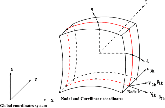
Shell element with various coordinates system


3.1 Element geometry and displacement field
In the isoparametric formulation, the coordinates of a point within an element are obtained as
where
and h k is the shell thickness at the node k.
Taking into consideration the two shell assumptions of the degeneration process, the displacement field is described by the five degrees of freedom of a normal viz. the three displacements of its mid-point \( \left( {\begin{array}{*{20}c} {u_{k} } & {v_{k} } & {w_{k} } \\ \end{array} } \right)^{T} _{mid} \) and two rotations \( \left( {\beta _{1k}, \beta _{2k} } \right). \) The displacements of a point on the normal resulting from the two rotations are calculated as
where u k , v k , w k are the displacements of node k on the mid-surface along the global X, Y, Z directions respectively, and N K is the shape function at kth node.
3.2 Strain displacement relations
Neglecting normal strain component in the thickness direction, the five strain components in the local coordinate system are given by
The local derivatives are obtained from the global derivatives of the displacements u, v and w using the transformation matrix. The derivatives of displacements of any point in the shell space with respect to curvilinear coordinates can be determined by using the displacement field described in Eq. 2. With the displacement derivatives, the strain displacement matrix in global coordinates can be formed. If \( \left\{ {d_{k}^{e} } \right\} = \left\{ {\begin{array}{*{20}c} {u_{k} } & {v_{k} } & {w_{k} } & {\beta _{1k} } & {\beta _{2k} } \\ \end{array} } \right\}^{T} \) is the vector of nodal variables corresponding to kth node of the element, the generalized nodal variables of an element \( \left\{ {d^{e} } \right\} \) is expresses as
The strain displacement equation relating the strain components {ε} in global coordinate system to the nodal variables {d e} is expressed as
The stress–strain relation in the global coordinate system can be written as
where \( \left\{ \sigma \right\} = \left[ {\begin{array}{*{20}c} {\sigma _{x} } & {\sigma _{y} } & {\tau _{xy} } & {\tau _{xz} } & {\tau _{yz} } \\ \end{array} } \right]^{T} \) are the stress components and [C] is the elastic constitutive matrix in global coordinate system. The elastic constitutive matrix in global coordinate system is given by
[C′] is the elastic constitutive matrix in material coordinate system and it can be obtain as follows.
where,
and k is the shear correction factor. Where [T m ] is the transformation matrix which transforms the elasticity matrix in the material axis system to the global coordinate system. The transformation matrix [T m ] is given by
where c = cos θ, s = sin θ and θ is the angle between the material axis and global axis.
3.3 Direct and converse piezoelectric relations
The linear piezoelectric constitutive equations coupling the elastic and electric fields can be respectively expressed as the direct and converse piezoelectric equations given by
where {D} denotes the electric displacement vector, {σ} denotes the stress vector, {ε} denotes the strain vector and {E} denotes the electric field vector. Further [e] = [d][C], where [e] comprises the piezoelectric coupling constants, [d] denotes the piezoelectric constant matrix and \( \left[ \in \right] \) denotes the dielectric constant matrix.
3.4 Electrical potential in the piezoelectric patch
The element has been assumed with one electrical degree of freedom at the top of the piezoelectric actuator and sensor patches, \( \phi _{a}^{e} \) and \( \phi _{s}^{e} \) respectively. Electrical potential has been assumed to be constant over an element and vary linearly through the thickness of piezoelectric patch. For a thin piezoelectric patch, the component of the electric field in the thickness direction is dominant. Therefore, the electric field can be accurately approximated with a non-zero component only in the thickness direction. With this approximation, the electric field strengths of an element in terms of the electrical potential for the actuator and the sensor patches respectively are expressed as
where subscripts a and s refer to the actuator patch and the sensor patch, respectively. The superscript e denotes the parameter at the element level. \( \left[ {B_{a}^{e} } \right] \) and \( \left[ {B_{s}^{e} } \right] \) are the electric field gradient matrices of the actuator and the sensor elements respectively. It should be noted that the electric potential is introduced as an additional degree of freedom on an element level.
3.5 Dynamic finite element equations
The dynamic equations of a piezo-laminated composite shell can be derived from the Hamilton principle
where L represents the Lagrangian, and δW is the virtual work of external forces. After the application of the variational principle and finite element discretization, the coupled finite element matrix equation derived for a one-element model becomes
Considering a laminate made up of N layers with a total thickness of T (as shown in Fig. 2), the elemental mass and transformed stiffness matrices can be written as
Structural mass: \( \left[ {M_{uu}^{e} } \right] = \int\nolimits_{V} {\rho \left[ {N^{T} } \right]\left[ N \right]} dV \)
Structural stiffness:
Dielectric conductivity of sensors/actuators:
Piezoelectric coupling matrix of sensors/ actuators:
Stiffness matrices have been evaluated by numerical integration using Gauss quadrature (3 × 3 × 2) scheme or (2 × 2 × 2) selective integration scheme depending on the shell thickness. After assembling the elemental stiffness matrices, the global set of equations become
For open electrodes, charge can be expressed as
After substituting Eqs. 19 and 20 in Eq. 18, the overall dynamic finite element equation can be expressed as
where [M uu ] is the global mass matrix, [K uu ] is the global elastic stiffness matrix, [K ua ] and [K us ] are the global piezoelectric coupling matrices of actuator and sensor patches respectively. [K aa ] and [K ss ] are the global dielectric stiffness matrices of actuator and sensor patches respectively.
3.6 State space representation
Lower order modes of vibration have lower energy associated and consequently are the most easily excitable ones. These are the most significant to the global response of the system. A truncated modal matrix ψ can be utilized as a transformation matrix between the generalized coordinates d(t) and the modal coordinates η(t). Thus the displacement vector d(t) can be approximated by the modal superposition of the first ‘r’ modes as
where [ψ] = [ψ1ψ2………ψ r ] is the truncated modal matrix.
Equation 22 can be rewritten as
where [M] = [M uu ]
The decoupled dynamic equations considering modal damping can be written as
where ξ di is the damping ratio. Equation 26 can be represented in state-space form as
where, \( \left[ A \right] = \left[ {\begin{array}{*{20}c} {\left[ 0 \right]} & {\left[ I \right]} \\ {\left[ { - \omega _{i}^{2} } \right]} & {\left[ { - 2\xi _{di} \omega _{i} } \right]} \\ \end{array} } \right] \) is the system matrix, \( \left[ B \right] = \left[ {\begin{array}{*{20}c} {\left[ 0 \right]} \\ { - \left[ \psi \right]^{T} \left[ {K_{ua} } \right]} \\ \end{array} } \right] \) is the control matrix, \( \left[ {\hat{B}} \right] = \left[ {\begin{array}{*{20}c} {\left[ 0 \right]} \\ {\left[ \psi \right]^{T} \left\{ F \right\}} \\ \end{array} } \right] \) is the disturbance matrix, {u d } is the disturbance input vector, {ϕ a } is the control input, and
The sensor output equation can be written as
where output matrix [C 0] depends on the modal matrix [ψ] and the sensor coupling matrix [K us ].
4 Controllability index for actuator location
The system controllability is a basis in the modern control theory. Wang and Wang (2001) proposed a controllability index for actuator locations, which was obtained by maximizing the global control force, and this has been considered in the present study. The modal control force f c applied to the system can be written as
It follows from Eq. 30 that
Using the singular value analysis, [B] can be written as [B] = [M][S][N]T where [M]T[M] = [I], [N]T[N] = [I] and
where n a is the number of actuators. Equation 31 can be rewritten as
Thus, maximizing this norm independently on the input voltage {ϕ a } induces maximizing \( \left\| S \right\|^{2}. \) The magnitude of σ i is a function of location and the size of piezoelectric actuators. Wang and Wang (2001) proposed that the controllability index is defined by
A similar controllability index can be proposed considering residual modes of system/structures and it can be maximized as follows
where \( \sigma _{i}^{R} \) are the components of [S R] corresponding to residual modes and γ′ is a weight constant.
5 LQR optimal feedback
Linear quadratic regulator optimal control theory has been used to determine the control gains. In this, the feedback control system has been designed to minimize a cost function or a performance index, which is proportional to the required measure of the system’s response. The cost function used in the present case is given by
where [Q] and [R] are the semi-positive-definite and positive-definite weighting matrices on the outputs and control inputs, respectively.
The steady-state matrix Ricatti equation can be written as
After solving the Ricaati equation using Potters method, optimal gain can be written as
Considering output feedback, actuation voltage can be calculated as
5.1 Determination of weighting matrices
Weighting matrices [Q] and [R] are important components of LQR optimization process. The compositions of [Q] and [R] elements influence the system’s performance. Lewis (1986) assumed [Q] and [R] to be a semi-positive definite and positive definite matrix respectively. Ang et al. (2002) proposed that [Q] and [R] matrices could be determined considering weighted energy of the system as follows
The proposed weighted energy of the system in the quadratic form is
where, α 1, α 2 and γ are the coefficients associated with total kinetic energy, strain energy and input energy respectively. These coefficients will take different values in the control algorithm apart from the value of unity to allow for the relative importance of these energy terms. The closed loop damping values can be calculated by using the following equation.
Therefore, a search algorithm is required for finding [Q] and [R] by taking α 1, α2 and γ as variables, which will give maximum control response within the allowable actuators voltage. In this present study, optimization problem has been formulated as follows
Subjected to
where \( p = \ln ( {\frac{{x_{i} }}{{x_{i + 1} }}} ), \) n a is the number of actuators and ϕ max refers to the maximum voltage that can be applied on the actuators depending on the piezoelectric materials and thickness of the piezolayers. The allowable voltage of piezo-ceramic materials is around 500–1000 V per 1 mm piezo thickness (Bruch et al. 2002).
6 Genetic algorithms (GA)
GA is a powerful and broadly applicable stochastic search and optimization technique based on the principles of natural selection and genetics. GA begins with a population of randomly generated candidates and evolves towards a solution by applying genetic operators such as reproduction, crossover and mutation. These algorithms are highly parallel, guided random adaptive search techniques. In the present study, two types of GAs have been used for optimal placement of actuators and finding [Q] and [R] matrices. In the following subsections, these algorithms have been briefly described.
6.1 Integer coded genetic algorithm
In the present problem the design variables are the positions of the actuators, and are represented in a string of integers specifying the locations of actuators. The gene code is taken as \( ac_{1} ,ac_{2} , \ldots \ldots ,ac_{j} , \ldots \ldots ,ac_{{n_{a} }},\) where \( ac_{j} \in (1,m) \) and is a positive integer number and m is the total locations for actuators in the structures/system. Uniform crossover and new mutation techniques for integer coded GA have been discussed in the following subsections.
6.1.1 Uniform crossover
The steps involve in this crossover are
-
(a)
A random mask is generated
-
(b)
The mask determines which bits are copied from one parent and which from the other parent
-
(c)
Bit density in mask determines how much material is taken from the other parent
For example, if the randomly generated mask is 0110011000 and parents are1010001110 and 0011010010 then their offspring will be 0011001010 and 1010010110.
6.1.2 Mutation
A one-digit positive integer value \( ac_{j} \in [1,m] \) is generated randomly, which replaces the old one when mutating. If ac j is equal to old one then a new positive integer is selected again until they are different in the chromosome. The efficiency of the mutation could be improved greatly using the method.
6.2 Real coded genetic algorithm
In the present study, real coded GA along with SBX and parameter based mutation (Deb and Gulati 2001) operators have been used for finding [Q] and [R] matrices in LQR control scheme. In the following subsections, these operators have been briefly described.
6.2.1 Simulated binary crossover (SBX)
A probability distribution function has been used around the parent solutions to create two children solutions as
where, \( \beta = | {\frac{{b^{(2)} - b^{(1)} }}{{a^{(2)} - a^{(1)} }}} | \) and b (1), b (2) are the children solutions, and a (1), a (2)are the parent solutions.
η c is a parameter which controls the extent of spread in children solution. A small value of η c allows solutions far away from parents to be created as children solutions and a large value restricts only near-parent solutions to be created as children solutions.
6.2.2 Parameter-based mutation operator
A polynomial probability distribution has been used to create a solution b in the vicinity of a parent solution as
\( \bar{\delta } \) is calculated as follows
where \( \delta = { \min }[(a - a^{l} ),(a^{u} - a)]/(a^{u} - a^{l} ) \) \( \eta _{m} \) is the distribution index for the mutation and takes any non-negative value.
Here 0 < u < 1 is generated at random and Δmax is maximum perturbation allowed in the parent solution.
6.3 Optimal actuator location using GA
The most natural representation is a string of integers specifying the locations of actuators has been used in this study, an integer coded GA with uniform crossover and mutation have been developed for optimal placement of actuators. The fitness value i.e. measure of controllability for the optimal actuators location has been proposed as follows
The outline of optimization problem using GA is as follows:
-
(i)
Initial chromosomes depending on the number of actuators and populations are chosen randomly.
-
(ii)
The fitness value (measure of controllability) is calculated for each chromosome.
-
(iii)
Genetic operators are applied to produce a new set of chromosomes.
-
(iv)
Steps (ii)–(iii) are repeated until convergence of fitness.
-
(v)
The computation is terminated after convergence of fitness and the chromosome based on the best controllability value is selected as the optimal locations of actuators.
Several important parameters used in genetic search are taken as follows: population size = 10; length of chromosome = number of actuators to be considered (n a ); crossover probability = 0.9; mutation probability = 0.1; γ′ = 0.1.
6.4 The GA approach to optimal LQR
In the present work, weighting matrices have been determined by the genetic search to obtain best control gain for the optimal LQR scheme. Parameters α 1, α 2 and γ in Eq. 39 have been represented by real-valued genes for finding [Q] and [R] matrices. The population size in the present problem has been taken as 10. The fitness value has been calculated with respect to each chromosome using the following expression.
The ranges of α 1, α 2 and γ are taken as 0 < α 1 ≤ 200, 0 < α2 ≤ 200 and 0 < γ ≤ 2 where controlled response d(t) Controlled response depends on α 1, α 2 and γ. Parents have been selected through roulette wheel operator and offspring have been created using SBX and polynomial mutation operator (Deb and Gulati 2001). The distribution parameters associated with SBX and polynomial mutation operator have been taken as η c = 2 and η m = 100. Genetic evolution has been continued for large number of generations till the fitness converges. Figure 4 shows the steps in determining the weighting matrices for optimal gain by real coded GA in the present problem.

Flowchart of GA based LQR
7 Results and discussions
Based on the above eight noded-layered shell element formulation with LQR control strategy and GA, a computer code has been developed for the present study. The following validations have been done for structural and electro-mechanical responses.
7.1 Structural validation
In order to verify the finite element code developed, the following parameters were used for a spherical shell made of graphite/epoxy. Dimensions of spherical shell: a/b = 1, R 1 = R 2 = R, R/a = 3, a/h = 10 with the four edges simply supported; Graphite/epoxy properties: E 1 = 25E 2, G 12 = G 13 = 0.5E 2, υ 12 = 0.25, G 23 = 0.2E 2. A 10 × 10 finite element mesh has been used to model this entire shell. Nondimensionalized central deflection (w a) of laminated spherical shell under point load P = 10 N at the center and nondimensionalized fundamental frequency (λ**) have been calculated from the present code are listed in Table 1 along with exact solution of Reddy (1984). Nondimensionalized central deflection (w a) and fundamental frequency (λ**) have been calculated using the following expressions
It could be observed that the results obtained from the present finite element code are in close agreement with the exact solution (Reddy 1984).
7.2 Electro-mechanical validation
In order to verify the accuracy of the present coupled electro-mechanical finite element code, the results obtained from the present code have been compared with the benchmark problem proposed by Hwang and Park (1993). Here, a cantilever bimorph (as shown in Fig. 5) made of two PVDF layers laminated together has been considered subjected to an external voltage. The induced internal stresses result in a bending moment which forces the bimorph beam to bend. The bimorph beam has been discretized into five elements. The dimensions of the beam are length, L = 100 mm, width, W = 5 mm and thickness, h = 1 mm. The analytical solution to transverse displacement w is given by Tzou and Ye (1996)

Schematic view of a bimorph beam
A unit voltage has been applied across the thickness and the calculated transverse deflections of five nodes have been compared with the results of Hwang and Park (1993), Tzou and Ye (1996) and Chee et al (1999) as shown in Table 2 and it could be observed that excellent agreements have been achieved.
7.3 Combined GA based optimal placement and LQR control scheme
After validation of the developed code, a simply supported smart FRP composite spherical shell panel on a square base (a = b = 0.04 m) under the action of impulse load at the center has been analyzed to study the optimal placement of actuators and vibration control. The radii (i.e. R 1 = R 2 = R) of this panel have been considered to be 0.12 m. Thickness of each ply has been considered as 0.75 mm and that of piezo patch is 0.5 mm. The stacking sequence of the laminated spherical structure considered is [p/[0/90]s/p]]. Here ‘p’ stands for piezo-patches one for sensing and the other for actuation. A 10 × 10 finite element mesh has been considered to model this entire panel. Optimal actuators placement and dynamic responses of the piezo-laminated structures have been calculated considering the first eight modes. First four modes out of eight modes have been considered as control modes and others have been considered as residual modes. Dynamic responses of the piezo-laminated structures have been calculated using mode superposition technique. In this study, six numbers of actuators have been considered. It has been assumed that the number of piezoelectric actuators to be less than the number of modes to be controlled (Wang and Wang 2001). In this study, a modal damping ratio (ξ d ) of 1% has been assumed to obtain open loop response and to calculate LQR gains (Bhattacharya et al. 2002). The allowable voltage of piezo-ceramic materials has been taken as 500 V (Bruch et al. 2002). The mechanical, electrical and coupled material properties (Bhattacharya et al. 2002) used in the present study have been listed in the Table 3.
Recently, GA based LQR control scheme has been developed for superior vibration control of smart structures (Roy and Chakraborty 2008). In order to study the variation of maximum actuator/input voltage and closed loop damping ratio on the actuators placement without or with control spillover using GA-LQR control scheme, two types of piezo patch locations viz. Placement 1 and Placement 2 have been considered. Placement 1 stands for optimal actuators placement based on the maximum controllability index neglecting control spillover as shown in Fig. 6. Figure 7 presents the evolution of the best fitness value i.e. controllability index using GA after 50 generations using Placement 1. Placement 2 stands for optimal actuators placement based on the maximum controllability index considering control spillover of the higher order modes as shown in Fig. 8. Figure 9 presents the evolution of the best fitness value i.e. controllability index using GA after 50 generations using Placement 2 considering first four modes as control modes. In all the cases, the smart panel has been subjected to an impulse load of 10 N at the center for a duration of τmin/25 s (where τmin is the time period corresponding to first natural frequency of the system) and impulse responses of this panel have been calculated with a time step of τmin/100 s. Figure 10 shows the uncontrolled displacement history of smart spherical panel. Figure 11 shows the comparison of GA-LQR controlled displacement history using Placement 1 and Placement 2. In this case the closed loop damping ratios for Placement 1 and Placement 2 are 12.03% and 16.69% respectively. The comparison of maximum actuator voltage variation using Placement 1 and Placement 2 for GA-LQR control scheme is shown in Fig. 12. Figure 13 shows the convergence of calculated fitness i.e. closed loop damping ratio with number of generation using Placement 1 and GA-LQR search control scheme. Figure 14 shows the convergence of calculated fitness i.e. closed loop damping ratio with number of generation using Placement 2 and GA-LQR search control scheme. It could be observed from the Fig. 11, 12 and 14 that combined GA based optimal placement considering control spillover of the higher order modes and LQR control scheme lead to increase closed loop damping ratio with a large reduction of input/actuator voltage.

Collocated sensors and actuators location on the spherical panel substrate based on the Placement 1

Variation of controllability index with generation using Placement 1

Collocated sensors and actuators location on the spherical panel substrate based on the Placement 2

Variation of controllability index with generation using Placement 2

Uncontrolled displacement history of the smart FRP composite spherical panel considering first eight modes

Comparison of GA-LQR controlled displacement history using Placement 1 and Placement 2

Comparison of maximum actuator voltage variation for GA-LQR control scheme using Placement 1 and Placement 2

Variation of closed loop damping ratio with generation using Placement 1 and GA-LQR control scheme

Variation of closed loop damping ratio with generation using Placement 2 and GA-LQR control scheme
8 Conclusion
In the present work an improved GA based combined optimal placement of piezoelectric actuators considering control spillover and LQR control scheme has been developed for optimal control of smart FRP composite shell structures while keeping the input voltages of the actuators within the limit. This combined module has been used in conjunction with the developed layered shell finite element procedure for coupled electromechanical analysis of smart shell structures. The combined GA based optimal placement by minimizing control spillover of the higher order modes and optimal control modules show superior performance in terms of closed loop damping ratio and settling time with a large reduction of control effort or actuation voltage. It can be concluded that this combined module could be used as a design tool for optimal vibration control of smart FRP composite structures.
References
Abdullah, M.M., Richardson, A., Hanif, J.: Placement of sensors/actuators on civil structures using genetic algorithms. Earthquake Eng. Struct. Dynam. 30(8), 1167–1184 (2001). doi:10.1002/eqe.57
Ahamad, S., Irons, B.M., Zienkiewicz, O.C.: Analysis of thick and thin shell structure by curved elements. Int. J. Numer. Meth. Eng. 2, 419–451 (1970). doi:10.1002/nme.1620020310
Ang, K.K., Wang, S.Y., Quek, S.T.: Weighted energy linear quadratic regulator vibration control of piezoelectric composite plates. J. Smart Mater. Struct. 11, 98–106 (2002). doi:10.1088/0964-1726/11/1/311
Bailey, T., Hubbard, J.E.: Distributed piezoelectric polymer active vibration control of a cantilever beam. J. Guid. Control Dyn. 85, 605–611 (1985). doi:10.2514/3.20029
Balagurugan, V., Narayanan, S.: Active vibration control of smart shells using distributed piezoelectric sensors and actuators. Smart Mater. Struct. 10, 173–180 (2001). doi:10.1088/0964-1726/10/2/301
Balagurugan, V., Narayanan, S.: A piezoelectric higher-order plate finite for the analysis of multi-layer smart composite laminates. Smart Mater. Struct. 16, 2026–2039 (2007). doi:10.1088/0964-1726/16/6/005
Balagurugan, V., Narayanan, S.: A piezolaminated composite degenerated shell finite element for active control of structures with distributed piezosensors and actuators. Smart Mater. Struct. 17, 015031 (18 pp) (2008)
Bhattacharya, P., Suhail, H., Sinha, P.K.: Finite element analysis and distributed control of laminated composite shells using LQR/IMSC approach. Aerosp. Sci. Technol. 6, 273–281 (2002). doi:10.1016/S1270-9638(02)01159-8
Bruch, J.C., Sloss, J.M., Sadek, I.S.: Optimal piezo-actuator locations/lengths and applied voltage for shape control of beams. J. Smart Mater. Struct. 9, 205–211 (2002)
Chee, C.Y.K., Tong, L., Steven, G.P.: A mixed model for composite beams with piezoelectric actuators and sensors. J. Smart Mater. Struct. 8, 417–432 (1999). doi:10.1088/0964-1726/8/3/313
Chen, S.H., Yao, G.F., Huang, C.: A new intelligent thin shell element. J. Smart Mater. Struct. 9, 10–18 (2000). doi:10.1088/0964-1726/9/1/302
Christensen, R.H., Santos, I.F.: Design of active controlled rotor-blade systems based on time-variant modal analysis. J. Sound Vibrat. 280, 863–882 (2005). doi:10.1016/j.jsv.2003.12.046
Crawley, E.F., Luis, J.: Use of piezoelectric actuators as elements of intelligent structures. AIAA J. 25(10), 1373–1385 (1987). doi:10.2514/3.9792
Deb, K., Gulati, S.: Design of truss-structures for minimum weight using genetic algorithms. Finite Elem. Anal. Des. 37, 447–465 (2001). doi:10.1016/S0168-874X(00)00057-3
Guo, H.Y., Zhang, L., Zhang, L.L., Zhou, J.X.: Optimal placement of sensors for structural health monitoring using improved genetic algorithm. J. Smart Mater. Struct. 13, 528–534 (2004). doi:10.1088/0964-1726/13/3/011
Han, J.H., Lee, L.: Optimal placement of piezoelectric sensors and actuators for vibration control of a composite plate using genetic algorithms. J. Smart Mater. Struct. 8, 257–267 (1999). doi:10.1088/0964-1726/8/2/012
Hiramoto, K., Doki, H., Obinata, G.: Optimal sensor/actuator placement for active vibration control using explicit solution of algebraic Riccati equation. J. Sound Vibrat. 229(5), 1057–1075 (2000). doi:10.1006/jsvi.1999.2530
Hwang, W.S., Park, H.C.: Finite element modeling of piezoelectric sensors and actuators. AIAA J. 31(5), 930–937 (1993). doi:10.2514/3.11707
Kang, Y.K., Park, H.C., Kim, J., Choi, S.B.: Interaction of active and passive vibration control of laminated composite beams with piezoceramics sensors/actuators. Mater. Des. 23, 277–286 (2002)
Kulkarni, S.A., Bajoria, K.M.: Finite element modeling of smart plates/shells using higher order shear deformation theory. Compos. Struct. 62, 41–50 (2003). doi:10.1016/S0263-8223(03)00082-5
Kusculuoglu, Z.K., Royston, T.J.: Finite element formulation for composite plates with piezoelectric layers for optimal vibration control applications. J. Smart Mater. Struct. 14, 1139–1153 (2005). doi:10.1088/0964-1726/14/6/007
Lee, C.K.: Theory of laminated piezoelectric plates for the design of distributed sensors/actuators Part 1: governing equations and reciprocal relationships. J. Acoust. Soc. Am. 87(3), 1144–1158 (1990). doi:10.1121/1.398788
Lee, S., Goo, N.S., Park, H.C., Yoon, K.J., Cho, C.: A nine- node assumed strain shell element for analysis of a coupled electro-mechanical system. Smart Mater. Struct. 12, 355–362 (2003). doi:10.1088/0964-1726/12/3/306
Lewis, F.L.: Optimal control. Wiley, New York (1986)
Li, Q.S., Liu, D.K., Tang, J., Zhang, N., Tam, C.M.: Combinatorial optimal design of number and positions of actuators in actively controlled structures using genetic algorithm. J. Sound Vibrat. 270, 611–624 (2004). doi:10.1016/S0022-460X(03)00130-5
Liu, W., Hou, Z.K., Demetriou, M.A.: A computational scheme for the optimal sensor/actuator placement of flexible structures using spatial H-2 measures. Mech. Syst. Signal Process. 20(4), 881–895 (2006). doi:10.1016/j.ymssp.2005.08.030
Marinković, D., Köppe, H., Gabbert, U.: Degenerate shell element for geometrically nonlinear analysis of thin-walled piezoelectric active structures. Smart Mater. Struct. 17, 015030 (10 pp) (2008)
Narayanan, S., Balamurugan, V.: Finite element modeling of piezolaminated smart structures for active vibration control with distributed sensors and actuators. J. Sound Vibrat. 262, 529–562 (2003). doi:10.1016/S0022-460X(03)00110-X
Nguyen, Q., Tong, L.: Voltage and evolutionary piezoelectric actuator design optimisation for static shape control of smart plate structures. Mater. Des. 28, 387–399 (2007)
Ram, K.S.S., Kiran, S.K.: Static behavior of laminated composite spherical shell cap with piezoelectric actuators. Smart Mater. Struct. 17, 015010 (9 pp) (2008)
Ray, M.C., Bhattacharyya, R., Samanta, B.: Static analysis of intelligent structure by the finite element method. Comput. Struc. 52(4), 617–631 (1994). doi:10.1016/0045-7949(94)90344-1
Reddy, J.N.: Exact solution of moderately thick laminated shells. J. Eng. Mech. 110(5), 794–809 (1984)
Robandi, I., Nishimori, K., Nishimura, R., Ishihara, N.: Optimal feedback control design using genetic algorithm in multimachine power system. Electr. Power Energy Syst. 23, 263–271 (2001). doi:10.1016/S0142-0615(00)00062-4
Roy, T., Chakraborty, D.: GA-LQR based optimal vibration control of smart FRP composite structures with bonded PZT patches. J. Reinforced Plastics Composites (2008). doi:10.1177/0731684408089506
Sadri, A.M., Wright, J.R., Wynne, R.: Modeling and optimal placement of piezoelectric actuators in isotropic plates using genetic algorithm. J. Smart Mater. Struct. 8, 490–498 (1999). doi:10.1088/0964-1726/8/4/306
Saravanos, D.A., Christoforou, A.P.: Impact response of adaptive piezoelectric laminated plates. AIAA J. 40(10), 2087–2095 (2002)
Swann, C., Chattopadhyay, A.: Optimization of piezoelectric sensor location for delamination detection in composite laminates. Eng. Optim. 38(5), 511–528 (2006). doi:10.1080/03052150600557841
Tzou, H.S., Tsang, C.I.: Distributed piezoelectric sensor/actuator design for dynamic measurement/control of distributed parameter systems: a finite element approach. J. Sound Vibrat. 138(1), 17–24 (1990). doi:10.1016/0022-460X(90)90701-Z
Tzou, H.S., Ye, R.: Analysis of piezoelectric structures with laminated piezoelectric triangle shell elements. AIAA J. 34, 110–115 (1996). doi:10.2514/3.12907
Wan, J.G., Tao, B.Q.: Design and study on a 1-3 anisotropy piezocomposite sensor. Mater. Des. 21, 533–536 (2000)
Wang, Q., Wang, C.: A controllability index for optimal design of piezoelectric actuators in vibration control of beam structures. J. Sound Vibrat. 242(3), 507–518 (2001). doi:10.1006/jsvi.2000.3357
Wang, S.Y., Tai, K., Quek, S.T.: Topology optimization of piezoelectric sensors/actuators for torsional vibration control of composite plates. J. Smart Mater. Struct. 15(2), 253–269 (2006)
Yang, Y., Jin, Z., Soh, C.K.: Integrated optimal design of vibration control system for smart beams using genetic algorithm. J. Sound Vibrat. 282, 1293–1307 (2005). doi:10.1016/j.jsv.2004.03.048
Zhang, N., Kirpitchenko, I.: Modelling dynamics of a continuous structure with a piezoelectric sensor/actuator for passive structural control. J. Sound Vibrat. 249(2), 251–261 (2002). doi:10.1006/jsvi.2001.3792
Zheng, S., Wang, X., Chen, W.: The formulation of refined hybrid enhanced assumed strain solid shell element and its application to model smart structures containing distributed piezoelectric sensors/actuators. Smart Mater. Struct. 13(43-N), 50 (2004)
Author information
Authors and Affiliations
Corresponding author
Rights and permissions
About this article
Cite this article
Roy, T., Chakraborty, D. Genetic algorithm based optimal design for vibration control of composite shell structures using piezoelectric sensors and actuators. Int J Mech Mater Des 5, 45–60 (2009). https://doi.org/10.1007/s10999-008-9085-z
Received:
Accepted:
Published:
Issue Date:
DOI: https://doi.org/10.1007/s10999-008-9085-z